


1. Introduction
The presence of a porous region in a channel alters the local flow field and generates large-scale coherent structures in its wake that modulate transport and mixing processes. One of the most important applications in environmental fluid mechanics is the case when the porous region corresponds to an aquatic canopy (Nepf Reference Nepf2012). Canopies in the form of patches of emerged and submerged vegetation are present in rivers and occupy different parts of the channel and its floodplain (Carr, Duthie & Taylor Reference Carr, Duthie and Taylor1997; Sukhodolov & Sukhodolova Reference Sukhodolov and Sukhodolova2010). Vegetation patches act as ecological engineers (Jones, Lawton & Schachak Reference Jones, Lawton and Schachak1994; Corenblit et al. Reference Corenblit, Gurnell, Steiger and Tabacchi2008; Gurnell Reference Gurnell2014) by generating regions with higher nutrient availability, deeper light penetration and higher plant productivity (Webster & Benfield Reference Webster and Benfield2003; Horppila & Nurminen Reference Horppila and Nurminen2003; Schultz et al. Reference Schultz, Kozerski, Pluntke and Rinke2003; Schoelynck et al. Reference Schoelynck, de Groote, Bal, Vandenbruwaene, Meire and Temmerman2012). Streams containing patches of vegetation have a superior capacity to sustain a high diversity of habitat (Beechie et al. Reference Beechie, Liermann, Pollock, Baker and Davies2006).
Vegetation patches reduce the transport capacity of the river due to the additional drag induced by the plants (Plew, Cooper & Callaghan Reference Plew, Cooper and Callaghan2008) and create regions of flow acceleration near some of the patch boundaries where bed erosion is substantial and nutrient availability is low (negative feedback for patch growth). The generation of near-bed turbulence by the patch also inhibits deposition and induces bed scouring, especially close to the front and sides of the patch (Pan et al. Reference Pan, Follett, Chamecki and Nepf2014; Kim, Kimura & Shimizu Reference Kim, Kimura and Shimizu2015; Yang, Chung & Nepf Reference Yang, Chung and Nepf2016). Deposition of fine sediment, organic matter and plant seeds and nutrient accumulation at the bed are generally enhanced inside vegetation patches and inside the low-energy regions at their backside (Gurnell et al. Reference Gurnell, Tockner, Edwards and Petts2005; Bouma et al. Reference Bouma, van Duren, Temmerman, Claverie, Blanco-Garcia, Ysebaert and Herman2007; van Wesenbeeck et al. Reference van Wesenbeeck2008; Schoelynck et al. Reference Schoelynck, de Groote, Bal, Vandenbruwaene, Meire and Temmerman2012). Deposition of these particulates increases bar sedimentation, promotes new plant growth, acts as a sink for carbon and nitrogen and raises ecosystem productivity (positive feedback for patch growth). When present near the channel banks, patches of vegetation reduce bank erosion.
Patch configuration and composition change over time in response to hydrologic and seasonal events (Malard et al. Reference Malard, Tockner, Dole-Olivier and Ward2002; Wiens Reference Wiens2002). Such discrete macrophyte patches of finite length and width generally develop at locations where the bathymetry and flow patterns favour formation of regions of low bed shear stress and accumulation of nutrients. One such case is the formation of fairly long vegetation patches adjacent to the channel's banks. The effects of the vegetation patch on the surrounding flow, transport and bed morphodynamics change over time due to seasonal plant growth and significant fluvial disturbances induced by river management decisions (e.g. dam operation) and floods (Cotton et al. Reference Cotton, Wharton, Bass, Heppell and Wotton2006). A deeply submerged patch generally corresponds to an initial stage of aquatic vegetation and/or to high-flow (e.g. flood) conditions in the stream. Due to seasonal growth and/or occurrence of low-flow conditions in the stream, the patch submergence decreases and eventually the patch becomes emerged.
Most previous experimental and numerical studies of flow past idealized vegetation patches (e.g. plant flexibility is neglected and the plant stems are modelled as solid vertical cylinders) were conducted in open channels containing an isolated patch of uniform porosity (e.g. see White & Nepf Reference White and Nepf2007; Zong & Nepf Reference Zong and Nepf2011, Reference Zong and Nepf2012; Chen et al. Reference Chen, Ortiz, Zong and Nepf2012; Chang, Constantinescu & Tsai Reference Chang, Constantinescu and Tsai2017; Koken & Constantinescu Reference Koken and Constantinescu2020). These studies considered either a circular or rectangular patch positioned at the centre of a straight channel, or a long rectangular patch placed at one of the channel's banks.
Until recently, flow past submerged vegetated canopies and porous obstacles focused on the case where the patch spanned the whole width of the channel (e.g. see Sukhodolov & Sukhodolova Reference Sukhodolov and Sukhodolova2010; Sukhodolova & Sukhodolov Reference Sukhodolova and Sukhodolov2012a,Reference Sukhodolova and Sukhodolovb; Chen, Jiang & Nepf Reference Chen, Jiang and Nepf2013; Hamed et al. Reference Hamed, Sadowski, Nepf and Chamorro2017; Hamed & Chamorro Reference Hamed and Chamorro2018; Monti, Omidyeganeh & Pinelli Reference Monti, Omidyeganeh and Pinelli2019; Monti et al. Reference Monti, Omidyeganeh, Eckhardt and Pinelli2020). Flow past submerged circular arrays of vertical cylinders placed at the centre of on open channel were studied experimentally by Liu et al. (Reference Liu, Hu, Lei and Nepf2017) and numerically by Chang, Constantinescu & Tsai (Reference Chang, Constantinescu and Tsai2020).
For high-aspect-ratio emerged rectangular patches placed at one of the sidewalls, White & Nepf (Reference White and Nepf2007) have shown that the velocity profile inside the horizontal shear layer is asymmetric and has a two-layer structure (figure 1). The outer region on the open water side resembles a boundary layer, while the inner region of the shear layer contains a velocity inflection point situated close to the interface between the array and the open water side of the channel. The velocity variation inside the inner region can be well approximated by a hyperbolic tangent profile. The length scale for the penetration of the shear layer vortices inside the array, δI, can be calculated as the distance from the inflection point (y = y 0) to the location where the mean streamwise velocity inside the array becomes close to constant in the transverse direction (e.g.  $\bar{u} = {U_1}$). The outer-layer length scale defines the distance away from the array where the mean streamwise velocity approaches the mean free-stream velocity outside the shear layer on the open water side, U 2. White & Nepf (Reference White and Nepf2007), estimated this length scale as ${\delta _o} = ({U_2} - {U_m})/{(\textrm{d}\bar{u}/\textrm{d}y)_{y = ym}}$, where the effective boundary layer origin is situated at a lateral position y = ym where the mean streamwise velocity is $\bar{u}({y_m}) = {U_m}$. At this lateral position, the inner- and outer-layer slopes of the velocity profiles match. Both δI and δ 0 were found to initially increase with the distance from the front of the array. At larger distances from the front of the array, the rate of growth of the shear layer width on the free-stream side decayed significantly, indicating bed friction stabilization limited the growth of the shear layer vortices on the open water side, similar to a classical shallow mixing layer. Moreover, the shear layer vortices reached a close to constant lateral penetration width on the array side.
Sketch showing computational domain containing a rectangular array of solid cylinders at the right bank of a straight open channel. The flow depth in the open channel is D, the diameter of the cylinders is d, the height of the cylinders is h ≤ D and the incoming mean-flow velocity is U. The length and width of the patch are L = 36D and W = 1.6D, respectively. Also shown are the volumetric fluxes though a cross-section of the array situated at a distance x from the channel inlet, Qa(x) and through the upstream face of the array, Qau = Qa(x = 8D). The volumetric fluxes through the top face, Qat(x), and the side face, Qas(x), of the array are calculated in between the upstream face of the array (x = 8D) and the cross-section situated at a distance x from the channel inlet. The inset shows the randomized arrangement of the solid cylinders inside the patch and the variation of the mean streamwise velocity across the channel with the inner and outer layers of the horizontal shear layer. Their widths are δI and δo and their origins are situated at y = yo and y = ym, respectively. Also shown are the velocities outside of the inner and outer layers, U 1 and U 2, and the velocity Um at y = ym which is the lateral distance at which the inner- and outer-layer slopes of the velocity profiles match. The inflection point in the velocity profile is situated at y = y 0.

More recently, Lei & Nepf (Reference Lei and Nepf2021) investigated flow past a submerged vegetated patch of finite width placed at the centre of a straight channel. Experiments were conducted with both rigid circular cylinders and with very flexible blades attached to a rigid sheath. Experiments also included the limiting two-dimensional (2-D) case where the width of the patch was equal to the channel width. Their study proposed analytical models to predict the length of the initial adjustment region downstream of which the streamwise velocity inside the patch is close to constant (fully developed region) and of the mean streamwise velocity variation inside the initial adjustment region. The analytical models were found to predict well experimental and field data for both rigid and flexible vegetation. This configuration is directly relevant to the present investigation conducted for a submerged rectangular array of cylinders placed at one of the channel's banks. Formally, the present configuration corresponds to half of the domain in Lei & Nepf (Reference Lei and Nepf2021) experiments except that the symmetry plane of the channel is replaced by a zero-velocity sidewall.
Bed morphological changes induced by rectangular arrays of emerged and submerged rigid circular cylinders placed at a sidewall of a straight channel were investigated experimentally by Kim et al. (Reference Kim, Kimura and Shimizu2015). Their experiments were conducted for fairly low-aspect-ratio arrays (length to width ratio less than 5). The most severe scour was observed inside the open water region, near the lateral side of the array and near the leading edge of the array. For clear-water scour conditions, they found that the scouring and maximum scour depth inside these two regions were a function of the submergence ratio and increased with the non-dimensional flow blockage (e.g. the product between the non-dimensional frontal area per unit volume, a, and the width of the array, W).
Both the cases considered in the present work and the submerged (3-D) arrays of cylinders investigated by Lei & Nepf (Reference Lei and Nepf2021) are characterized by a more complex flow structure compared with the limiting cases of an emerged array, where a horizontal shear layer develops on the open water side, and of a submerged array extending over the whole channel width, where a vertical shear layer develops over the top of the array. In the case of a submerged array of vertical cylinders extending over a finite distance away from one of the channel's banks, both a horizontal and a vertical shear layer form. The large-scale eddies generated in the two shear layers are not independent, but the shear layers are expected to have a different dynamics and growth rate as the mean shear between the (free-stream) open water region and the porous region is generally not the same for the two shear layers. Moreover, the development of the vertical shear layer is constrained by the free surface, especially for low submergence cases, while the development of the horizontal shear layer vortices is constrained by bed friction effects at large distances from the origin of the shear layer (Finnigan Reference Finnigan2000; Sukhodolova & Sukhodolov Reference Sukhodolova and Sukhodolov2012a; Cheng & Constantinescu Reference Cheng and Constantinescu2020). Although the structure of the flow inside the horizontal shear layer was studied experimentally (White & Nepf Reference White and Nepf2007) and numerically (Koken & Constantinescu Reference Koken and Constantinescu2020) for emerged rectangular arrays, no such information is available for submerged arrays.
The present paper discusses the physics of flow past a rectangular array of vertical cylinders of height h placed at one of the sidewalls of an open channel (figure 1). In the case of submerged arrays, the height of the array, h, is smaller than the flow depth, D, such that the submergence ratio, D/h is larger than 1. The geometrical set-up of the present study is the same as the one used in the simulations of Koken & Constantinescu (Reference Koken and Constantinescu2020) conducted for emerged arrays and the experiments of White & Nepf (Reference White and Nepf2007). Two main parametric studies are conducted. In the first one, the effect of the array submergence is investigated for an array with a solid volume fraction ϕ = 0.08 and 1 ≤ D/h ≤ 4. The second parametric study investigates the effect of varying the solid volume fraction (0.02 ≤ ϕ ≤ 0.08) for a submerged array with D/h = 2.0.
The discussion is based on eddy-resolving numerical simulations that resolve the flow past the individual cylinders forming the array. This approach avoids the need to introduce additional empirical terms in the governing equation to account for the deceleration of the flow and generation of turbulence inside the porous region. This approach was used by Huai, Xue & Qian (Reference Huai, Xue and Qian2015), Chang et al. (Reference Chang, Constantinescu and Tsai2017, Reference Chang, Constantinescu and Tsai2020) and Liu et al. (Reference Liu, Huai, Ji and Han2021) to simulate flow past emerged and submerged arrays of cylinders situated away from the channel banks and by Koken & Constantinescu (Reference Koken and Constantinescu2020) to simulate flow past a rectangular array of emerged cylinders placed at one of the channel's sidewalls.
A major advantage of eddy-resolving simulations that resolve the flow past the individual cylinders is that they provide detailed data on the bed shear stress distributions outside and inside the array, on the forces acting on each cylinder and on the 3-D flow structure inside the array. These quantities are very difficult to accurately measure in flume experiments but are critical to provide a full understanding of the flow structure, to describe sediment erosion mechanisms and to characterize the spatial distribution of the additional drag induced by the cylinders forming the array. For example, it will be of interest to check if the observed patterns of severe bed erosion in the experiments of Kim et al. (Reference Kim, Kimura and Shimizu2015) are consistent with predicted regions of high bed shear stress in the mean and instantaneous flow fields in simulations conducted with a flat bed corresponding to the start of the erosion and deposition process. Moreover, analysis of the flow fields is not limited to one or a few horizontal planes, as is the case in most experimental studies, which allows us to characterize the vertical non-uniformity of the flow and the eventual presence of strong upwelling and downwelling motions inside the array and of cells of secondary flow outside it. Previous experimental studies provide only very limited information on 3-D effects and secondary flow motions. In the case of vegetation patches, these motions affect the distribution of nutrients and fine sediments inside the patch and the availability of nutrient rich soil to the plant roots. As for the case of a circular submerged array placed away from the channel's banks (Chang et al. Reference Chang, Constantinescu and Tsai2020), the recirculation region at the back of the array may shrink considerably, or disappear, with increasing submergence due to the flow advected over the top of the array. The capacity of the vegetated patch to grow is affected by the presence or not of a recirculation flow region at its back that favours deposition of particulates and nutrients.
The fact that the present study is conducted with arrays containing solid cylinders limits the direct extrapolation of the findings to applications involving submerged flexible aquatic plants (e.g. see Caroppi et al. Reference Caroppi, Västilä, Gualtieri, Järvelä, Giugni and Rowiński2021), especially if the vegetated canopies contain plants with highly flexible roots and lots of leaves. This is less of a concern for cases when the plant stems are more rigid and the contribution of the leaves and the other highly flexible parts of the plant to the total drag is relatively small. As such, it is reasonable to expect that flow structures (e.g. large shear layer eddies generated in the open water regions adjacent to the faces of the canopy) and large-scale secondary flow patterns triggered by the distributed drag associated with the plant stems (e.g. cylinders) will likely be similar for both rigid and flexible plants, given an equivalent distributed drag. On the other hand, flow structures triggered by separation around individual plant stems will likely be different if the plant stems are highly flexible and/or if their shapes are far from circular (e.g. vegetation types considered in the experiments with submerged patches and flexible plants conducted by Lei & Nepf Reference Lei and Nepf2021).
Specific objectives of the present study are to understand the effects of increasing the array's submergence and varying the solid volume fraction for constant submergence ratio on: (i) the distributions of the mean streamwise velocity and turbulent kinetic energy (TKE) inside the array and the adjacent open water regions; (ii) the spatial development and eddy structure of the horizontal and shear layer; (iii) the streamwise distribution of the average normal velocities and fluxes of fluid through the top and side surfaces of the array; (iv) flow separation in the wake of the array; (v) 3-D effects associated with upwelling and downwelling motions and formation of secondary cells on the open water side; (vi) the bed shear stresses and the capacity of the flow to entrain sediment inside and outside of the array; and (vii) the non-dimensional total streamwise drag force acting on the array and the spatial distribution of the non-dimensional drag forces acting on the individual cylinders.
Previous investigations conducted for emerged, rectangular, porous patches (e.g. White & Nepf Reference White and Nepf2007; Koken & Constantinescu Reference Koken and Constantinescu2020; Lei & Nepf Reference Lei and Nepf2021) and for submerged patches spanning the whole channel width (e.g. Chen et al. Reference Chen, Jiang and Nepf2013; Lei & Nepf Reference Lei and Nepf2021) have shown that the lateral and, respectively, the vertical flux, out of the porous region is high inside the initial adjustment region and negligible downstream of it. These studies also showed that once the horizontal/vertical shear layer and its penetration distance inside the array stabilize at the end of the initial adjustment region, the mean (cross-stream-averaged) streamwise velocity inside the array is close to constant. The same conclusion was reached by Lei & Nepf (Reference Lei and Nepf2021) for the streamwise velocity inside submerged rectangular patches placed at the centre of the channel. A main research question is to investigate if such a regime is also observed for submerged rectangular patches placed at one of the sidewalls of a channel and if this regime is associated, or not, with negligible fluxes through the top and lateral surfaces, something not investigated in previous experiments conducted for submerged patches.
Section 2 presents a brief description of the numerical method and boundary conditions. Section 3 discusses the main changes in the flow structure between cases with emerged and submerged arrays. The focus is on the coherent structures generated inside the patch and the horizontal shear layer, 3-D effects including generation of secondary (mean) flow cells and upwelling/downwelling motions, distribution of TKE and of the bed shear stresses and on the capacity of the flow to entrain sediment inside and around the patch. Section 4 analyses the effects of varying the submergence ratio for constant ϕ and of ϕ for constant D/h on the streamwise distributions of the mean streamwise velocity inside the array and in the two adjacent open water regions, and of the mean normal velocities through the top and side faces of the array. Section 5 analyses the same two effects related to varying D/h and ϕ on the TKE inside the array. Section 6 analyses the spatial distribution of the normalized streamwise drag forces acting on the cylinders and the total streamwise force acting on the array. Some final discussion and conclusions are provided in § 7.
2. Numerical model
The viscous flow solver (Chang, Constantinescu & Park Reference Chang, Constantinescu and Park2007a) solves the discretized incompressible Navier–Stokes equations in generalized curvilinear coordinates on a non-staggered grid and uses the detached eddy simulation (DES) approach to capture the dynamics of the energetically important eddies in the flow. The one-equation Spalart–Allmaras (SA) model is used as the base turbulence model. The turbulence length scale is redefined away from solid boundaries such that it becomes proportional to the cell size, which allows flow instabilities to develop, similar to large eddy simulation (LES). The delayed version of DES is used to avoid early transition to the LES mode inside the attached boundary layers. The Navier–Stokes equations are integrated using a fully implicit, fractional-step method. The convective terms in the momentum equations are discretized using a blend of the fifth-order accurate upwind-biased scheme and the second-order central scheme. The convective terms in the SA model transport equation are discretized using the second-order upwind scheme. The other terms in the governing equations are discretized using second-order central differences. The discrete momentum (predictor step) and turbulence model equations are integrated in pseudo-time using an alternate-direction-implicit approximate factorization scheme. Time integration is performed using a double time-stepping algorithm. The flow solver is used with grids that are fine enough to resolve the viscous sublayer such that no wall functions are used in the SA model.
Relevant validation studies include flow in flat-bed open channels (Koken, Constantinescu & Blanckaert Reference Koken, Constantinescu and Blanckaert2013), mixing layers forming in straight open channels (Constantinescu Reference Constantinescu2014; Cheng & Constantinescu Reference Cheng and Constantinescu2020) and flow past solid emerged cylinders (Kirkil & Constantinescu Reference Kirkil and Constantinescu2009, Reference Kirkil and Constantinescu2015; Zeng & Constantinescu Reference Zeng and Constantinescu2017). For the case of a circular porous patch containing an array of uniformly distributed, emerged cylinders, Chang et al. (Reference Chang, Constantinescu and Tsai2017) compared DES predictions of the mean velocity and lateral velocity fluctuations along the array's centreline with data from the experiments of Zong & Nepf (Reference Zong and Nepf2012) and Chen et al. (Reference Chen, Ortiz, Zong and Nepf2012) conducted with similar values of ϕ and observed good agreement. The predicted values of the Strouhal number associated with the anti-symmetric shedding mode in the wake of the array were within 5 % of the measured values. The simulations conducted by Koken & Constantinescu (Reference Koken and Constantinescu2020) for a rectangular array of emerged cylinders placed at a sidewall of an open channel showed that the development and turbulence structure of the shear layer forming at the lateral edge of the array were similar to those in the experiments conducted by White & Nepf (Reference White and Nepf2007). The same simulations accurately captured the distributions of the mean streamwise velocity and primary Reynolds stress inside the inner and outer regions of the horizontal shear layer.
In the simulations reported in the present study, the flow depth and the position of the array relative to the inlet an outlet sections are kept constant (figure 1). The channel Reynolds number of the incoming, fully developed, turbulent flow is also kept constant ( $R{e_D} = UD/\nu = 12\,500$, U is the mean velocity in the channel upstream of the array, ν is the molecular viscosity of the fluid). The length and width of the porous region are L = 36D and W = 1.6D, respectively. The solid volume fraction of the array, ϕ, is defined as the ratio between the total volume of the N solid cylinders forming the array and the volume of the array region. Given that the diameter d of the rigid cylinders is kept constant in all simulations (d = 0.1D) and the patch has uniform porosity and constant width, varying the array's solid volume fraction, $\phi = N{\rm \pi} {d^2}/4(WL)$, is equivalent to varying the non-dimensional frontal area per unit volume, $aW = (4/{\rm \pi} )(W/d)\phi$. The range of ϕ values (0.02 ≤ ϕ ≤ 0.08) in the simulations are representative for vegetation patches growing in rivers for which ϕ < 0.1 (Zong & Nepf Reference Zong and Nepf2012). The cylinder Reynolds number (Red = 1250) is sufficiently high for the flow to induce vortex shedding, at least for the cylinders situated close to the front of the array. The main geometrical parameters for each test case are summarized in table 1.
Main geometrical and flow variables of the test cases (ϕ is the solid volume fraction of the array, N is the number of cylinders in the array, d is diameter of the circular cylinders, D is the flow depth, W is the width of the array, ReD = UD/ν, Red = Ud/ν, a is the frontal area per unit volume for the array, Lsep is the length over which recirculation bubbles are present in the wake of the array, Xa is the length of the initial adjustment region inferred from the simulations, Xam is the length of the initial adjustment region predicted by (4.1),  ${\overline {\tilde{u}} _c}$ is the mean streamwise velocity inside the array for x > 8D + Xa, ${\bar{v}_c}$ is the mean spanwise velocity through the side face of the array in the equilibrium regime where ${q_{s - t}}$ is constant, ${\tilde{w}_c}$ is the mean vertical velocity through the top face of the array in the equilibrium regime).

The set-up of the simulations and the methodology to distribute the cylinders inside the array using a close-to-regular staggered pattern in the x–y planes are the same as those used by Koken & Constantinescu (Reference Koken and Constantinescu2020). A random displacement of 0.03D–0.06D was applied in both horizontal directions such that the solid cylinders of diameter are slightly displaced with respect to the regular staggered pattern (see inset in figure 1). The irregular arrangement of the cylinders reduces the regularity of the wake-to-cylinder interactions and the formations of corridors of high mean velocity inside the array (Chang & Constantinescu Reference Chang and Constantinescu2015). An irregular arrangement of the cylinders inside the array is also commonly adopted in most laboratory experiments (Liu et al. Reference Liu, Diplas, Fairbanks and Hodges2008; Follett & Nepf Reference Follett and Nepf2012) to avoid the generation of preferential directions of motion inside the array. The bed is located at z = 0, the free surface at z = D and the top of the solid cylinders at z = h. The origin of the system of coordinates is located at the channel inlet section on the right sidewall (figure 1). The front face of the array is situated at x = 8D. The exit section is situated at x = 59D. The width of the open channel is Wc = 4.8D. The width of the patch is W = 1.6D.
The flow entering the array through its front face can leave the array through its top and side faces. Flow from the open water regions can also enter the array through these two faces. Using continuity (see also figure 1), one can write  ${Q_{au}} = {Q_a}(x/D) + {Q_{as}}(x/D) + {Q_{at}}(x/D)$, where ${Q_a}(x/D)$ is the streamwise volumetric flux in the x = constant cross-section, ${Q_{au}} = {Q_a}(x/D = 8)$ and Qas and Qat are the volumetric fluxes through the top and side surfaces in between x = 8D (front face of the array) and the current cross-section, respectively.
The mesh in horizontal planes was identical to that in the corresponding emerged-array simulations discussed by Koken & Constantinescu (Reference Koken and Constantinescu2020). The number of points used to resolve the flow in vertical direction was increased from 48 to 64 in the simulations conducted with D/h > 1 to better resolve the flow close to the top face of the array where the interaction of the vertical shear layer with the submerged cylinders generates a large amount of smaller-scale turbulence. The level of mesh refinement was similar inside the horizontal and vertical shear layers. The first point off the channel bed and sidewalls was placed at 0.0015D from the no-slip surface, which corresponded to about one wall unit. Inside the array, the average grid spacing in the horizontal directions was close to 0.017D away from the surface of the solid cylinders. The wall-normal grid spacing was decreased to 0.0025D at the cylinders’ surface. Close to 36 grid points were placed on the circumference of each solid cylinder. Koken & Constantinescu (Reference Koken and Constantinescu2020) discuss requirements and additional simulations performed to ensure the flow inside the array was sufficiently well resolved. The LES mode became active starting at a distance of about 0.2d from the surface of the solid cylinders.
Following the procedure used by Chang, Constantinescu & Park (Reference Chang, Constantinescu and Park2007b), the incoming flow contained resolved turbulent fluctuations from a precursor eddy-resolving simulation performed in a straight channel of same height and width as the computational domain in figure 1. The length of the domain in the precursor simulation was 16D, no cylinders were present and periodic boundary conditions were used in the streamwise direction. In the simulations conducted with cylinders, a convective boundary condition was applied at the outflow. The free surface was modelled as a shear-free, rigid lid. The surfaces of the cylinders and channel walls were treated as no-slip, smooth walls. The time step was 0.001D/U. Mean flow and turbulence statistics were collected over a time interval of approximately 200D/U.
3. Main changes in flow and turbulence between cases with emerged and submerged arrays
3.1. Coherent structures generated inside and around the array
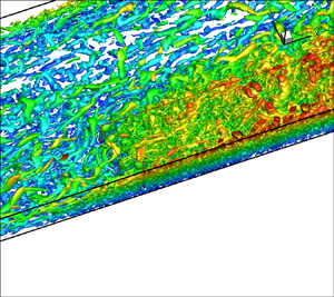
One of the main findings of the study conducted by Koken & Constantinescu (Reference Koken and Constantinescu2020) for emerged arrays of cylinders was that the advection of the horizontal shear layer vortices induces large-scale, wave-like oscillatory motions inside the array. Regions of high and low streamwise velocity and vertical vorticity form starting some distance from the front of the array. These regions extend over the whole width of the array. Figure 2(a) visualizes these regions for an emerged array with ϕ = 0.08. The frequency of these oscillatory motions is approximately half that associated with the advection of the horizontal shear layer vortices. Simulations conducted for submerged arrays with ϕ = 0.08 show that increasing the array submergence strongly dampens these oscillatory motions, such that these motions are suppressed for D/h ≥ 2.0 (figure 2b). The main reasons for the suppression of the oscillatory motions inside the array are the strong decay of the average size and coherence of the horizontal shear layer vortices, and the reduction of the lateral penetration distance of these vortices for high submergence array. These statements are supported by the analysis provided below.
Vertical vorticity, ωz(D/U), in the z/h = 0.5 plane (instantaneous flow): (a) ϕ = 0.08, D/h = 1.0; (b) ϕ = 0.08, D/h = 2.0. The red arrows in top panel point toward regions of high vorticity magnitude and high streamwise velocity inside and downstream of the array associated with long-amplitude, wave-like oscillations of the flow starting some distance from the front of the array.

The 2-D streamline patterns in figures 3(b) and 3(c) suggest a reduction in the size of the shear layer vortices and of their penetration distance inside the array with increasing D/h in the ϕ = 0.08 simulations with D/h ≥ 1.33. This is confirmed using the procedure proposed by White & Nepf (Reference White and Nepf2007) to estimate the position and width of the horizontal shear layer based on the mean velocity profiles at three streamwise locations (x/D = 14.5, 24.5 and 34.5). The estimated widths of the inner and outer layers, δI and δ 0, and of their origins y 0 and ym (figure 1) are then used to calculate the positions of the boundaries of the inner and outer layers with respect to the lateral face of the array (figure 3). The positions and widths of the shear layer eddies at these locations inferred from the 2-D streamlines in figure 3 are consistent with the boundaries of the inner and outer regions deduced based on the lateral profiles of the mean streamwise velocity. The largest rate of growth of the horizontal shear layer does not occur in the emerged case (figure 3a) but rather in the D/h = 1.33 case (figure 3b). For example, in the ϕ = 0.08 simulation, the width of the horizontal shear layer at x/D = 34.5 is 1.54D in the emerged case. The shear layer width increases to 1.93D in the D/h = 1.33 case. This increase is mainly due to the growth in δI. As a result, the lateral penetration distance of the eddies inside the array increases from 0.11D (D/h = 1.0) to 0.45D (D/h = 1.33). With further increase of the submergence ratio, the inner and outer regions of the shear layer shrink such that the shear layer width at x/D = 34.5 is 1.3D in the D/h = 2.0 case and only 0.75D in the D/h = 4.0 case.
Instantaneous flow 2-D streamline patterns in the z/h = 0.5 plane in a frame of reference moving with the mean advection velocity of the shear layer vortices: (a) ϕ = 0.08, D/h = 1.0; (b) ϕ = 0.08, D/h = 1.33; (c) ϕ = 0.08, D/h = 2.0. The red symbols show the boundaries of the inner and outer regions of the horizontal shear layer.

Analysis of the velocity power spectra and of the mean velocity inside the outer layer allows us to determine the frequency of passage of the larger shear layer vortices, fH, and the energy associated with the dominant frequency and to approximate the advective velocity of these vortices. For the ϕ = 0.08 simulations, the non-dimensional frequency associated with the passage of the shear layer vortices, StH = fHU/D, at x/D = 34.5 decreases from 0.19 for D/h = 1.0 to 0.14 for D/h = 1.33 before starting to increase with increasing submergence ratio. For D/h = 4.0, StH is close to 0.5. Using the advective velocity one can then estimate the average streamwise length of these vortices around x/D = 34.5. This length scale is close to 6D in the emerged case, 8.0D for D/h = 1.33 and 3.0D for D/h = 2.0. So, the average shape of these vortices is ellipsoidal. The aspect ratio is close to 4.0 in the emerged and low submergence case. It then decreases with increasing submergence ratio to reach about 2.5 for D/h = 2.0. The energy associated with StH decreases by more than one order of magnitude between D/h = 1.33 and D/h = 4.0, which indicates a clear reduction in the coherence of the shear layer vortices for high array submergence. This is consistent with the decay of the mean shear between the streamwise flow inside the array and the flow in the open channel region bordering the side face of the array with increasing D/h (see § 4.1).
The horizontal distributions of the TKE averaged over the height of the cylinders,  $\bar{k}/{U^2}$, in the ϕ = 0.08 simulations (figure 4) show high turbulence levels in between the lateral face of the array and the boundary of the outer region of the horizontal shear layer. The high TKE levels inside the outer layer are due to the passage of the shear layer vortices (figure 3). Interestingly, it is only in the D/h = 1.33 case (figure 4b) that TKE levels that are significantly higher than the ones in the incoming fully developed turbulent flow are observed inside the open water region, outside of the shear layer. This is due to the secondary cell forming on the open water side (see § 3.2). The circulation and distance between the core of this cell and the lateral face of the array are the largest in the D/h = 1.33 case. At locations where this cell is partially situated inside the outer region of the shear layer, some of the smaller eddies advected inside the shear layer can leave this region.
Averaged (0 < z < h) TKE,  $\bar{k}/{U^2}$, in a horizontal plane: (a) ϕ = 0.08, D/h = 1.0; (b) ϕ = 0.08, D/h = 1.33; (c) ϕ = 0.08, D/h = 2.0; (d) ϕ = 0.08, D/h = 4.0. The white symbols show the boundaries of the inner and outer regions of the horizontal shear layer.

Inside the array, relatively high TKE levels are observed inside the inner region of the shear layer. The high TKE levels are due to the passage of the larger-scale shear layer vortices penetrating inside the array and to the eddies shed by the cylinders situated close to the lateral face of the array. Away from the lateral face, the increase of the submergence ratio results in a decrease of the TKE close to the front face of the array. This is because the energy of the shed eddies scales with the mean velocity of the flow penetrating the array which decreases with increasing D/h (see § 3.2). Away from the front face, the length of the region where vortex shedding is observed increases with D/h, which explains the increase of the region measured from the front face of the array where the TKE levels are at least 100 % larger than the mean value in the flow approaching the array. This region extends until close to the back of the array in the ϕ = 0.08, D/h = 4.0 case (figure 4d). Its length is only 4D in the corresponding emerged case (figure 4a). The growth of the region containing cylinders that shed eddies is mainly due to the monotonic increase of the mean streamwise velocity inside the array with D/h. This velocity increase starts some distance from the front face of the array and peaks downstream of the initial adjustment region (see § 3.2).
A main difference between the emerged and submerged cases with ϕ = 0.08 is that, while the TKE levels are negligible at the back of the emerged patch, they are of the same order (generally approximately 50 % lower) as those recorded inside the downstream part of the horizontal shear layer in the submerged cases. This difference is because no recirculation bubble forms at the back of the patch in any of the submerged cases (figure 4).
As opposed to the case of non-porous obstructions placed at the lateral sidewall of an open channel (see e.g. Koken and Constantinescu Reference Koken and Constantinescu2008), no horseshoe vortices form around the upstream face of the emerged array in figure 5(a) where the coherent structures are visualized using the Q criterion (Dubief & Delcayre Reference Dubief and Delcayre2000) in the ϕ = 0.02, D/h = 1.0 simulation. (The Q variable is the second invariant of the resolved velocity gradient tensor and isolates regions where rotation dominates strain in the flow.) This is also the case for the other emerged-array cases with ϕ ≤ 0.08. As the array becomes submerged, part of the incoming flow approaching the front face is advected over the array. A reduced downflow should diminish the coherence of any horseshoe vortices forming around the front face. Indeed, no such horseshoe vortices form in any of the simulations conducted with submerged arrays (e.g. see figure 5(b) for the ϕ = 0.02, D/h = 2.0 simulation). However, some local scour is still going to be induced over the upstream part of the array by horseshoe vortices forming around the base of the individual cylinders that are directly or partially exposed to the incoming flow. These mean-flow vortices are visualized in figures 5(a) and 5(b). The coherence of these vortices increases with decreasing ϕ and/or decreasing D/h. In the case of a loose bed, the small scour holes around the individual cylinders can grow large enough to start merging, which may create a scour hole extending around part of the front face of the array (Kim et al. Reference Kim, Kimura and Shimizu2015). At that point, it is possible for horseshoe vortices to form around the upstream face of the array even for arrays with ϕ ≤ 0.08.
Visualization of the coherent structures around the upstream part of the array using the Q criterion: (a) ϕ = 0.02, D/h = 1.0, mean flow, view from above; (b) ϕ = 0.02, D/h = 2.0, mean flow, view from above; (b) ϕ = 0.08, D/h = 2.0, instantaneous flow, 3-D view. The red lines show the border of the array region.

The formation of the vertical shear layer is accompanied by the generation of large hairpin-like coherent structures. In the ϕ = 0.08 and 0.02 simulations with D/h ≤ 2.0, the largest of these eddies penetrate until the free surface (e.g. see figure 5c). For D/h = 4.0, these hairpins extend until z/D ≈ 0.85, which roughly corresponds to the top of the vertical shear layer in the mean flow. Such eddies are not generally observed inside the horizontal shear layer.
3.2. Streamwise momentum redistribution and secondary flow motions
Figure 6 compares the mean streamwise velocity distributions in the x/D = 35 section cutting through the downstream part of the array. In the emerged cases (e.g. see figure 6(a) for ϕ = 0.08), the streamwise velocity is fairly uniformly distributed over the flow depth both inside the array and inside the open water region. This is not the case anymore once the array becomes submerged. As D/h increases, the core of high streamwise velocity moves closer to the sidewall not containing the array and to the free surface. The fluid moving over the array is also faster than the one moving inside the array, where the flow is slowed down by the additional drag induced by the cylinders. This results in a very non-uniform distribution of the streamwise velocity inside the cross-section in submerged-array cases (e.g. see figure 6(b) for the ϕ = 0.08, D/h = 2.0 case).
Mean streamwise velocity, u/U, in the x/D = 35 cross-section cutting through the array: (a) ϕ = 0.08, D/h = 1.0; (b) ϕ = 0.08, D/h = 2.0. The solid and dashed line rectangles in (b) denote the open water regions situated adjacent to the top and side faces of the array, respectively.

The redistribution of the streamwise momentum in the cross-section due to the array becoming submerged is accompanied by the generation of cross-stream motions in the mean flow. In particular, flow downwelling occurs inside the open water region side of the horizontal shear layer, close to the lateral face of the array (figure 7). The strength of the downwelling motions inside this region peaks for low array submergences (e.g. for D/h = 1.33 in the ϕ = 0.08 simulations with 1.0 ≤ D/h ≤ 4.0). As illustrated by the mean vertical velocity distribution in the ϕ = 0.08 simulations with D/h = 1.33 (figure 7b) and D/h = 4.0 (figure 7c), significant flow upwelling is generated in the submerged-array cases in the wakes of the cylinders, with the strongest upwelling recorded for the cylinders situated near the lateral face of the array. So, the horizontal shear layer is far from behaving like a 2-D shear layer. This finding is relevant for patches of vegetation because it affects the dynamics of the nutrients and, in general, transport of particulates in between the open water region and the vegetation patch.
Mean vertical velocity,  $w/U$, in the z/h = 0.5 and x/D = 25.0 planes: (a) ϕ = 0.08, D/h = 1.0; (b) ϕ = 0.08, D/h = 1.33; (c) ϕ = 0.08, D/h = 4.0. The red rectangle shows the position of the array. The vertical dashed line shows the lateral face of the array. The main cross-stream cell of secondary flow is visualized using 2-D streamlines.

The other region of strong flow upwelling inside the submerged array corresponds to the wakes of the cylinders situated close to the front face of the array (figure 7b,c). Away from the front face, the mean vertical velocity magnitude inside the array is approximately 5–10 times smaller in the emerged case (figure 7a) compared with the submerged cases (figure 7b,c). Still, fairly strong upwelling and downwelling motions are present inside the upstream part of the array even if the array is emerged. The largest negative vertical velocities occur inside the downflow in front of the emerged array. This downflow region extends on the lateral side of the array in the region of strong flow acceleration forming as part of the incoming flow is deflected toward the open water side (figure 7a). Such a region of flow downwelling is also present in the submerged-array cases (figure 7b), but its size and the vertical velocity magnitude inside it decrease with increasing D/h as part of the flow approaching the front face of the array is advected over the array.
Another consequence of the redistribution of the streamwise momentum in the cross-section as the incoming flow reaches the submerged array and of strong turbulence anisotropy effects generated in between the array region and the open water regions is the generation of a streamwise-oriented cell of secondary flow parallel to the lateral face of the array. Its formation mechanism is similar to that of the secondary flow cells forming in compound channels (Shiono & Knight Reference Shiono and Knight1991). Even for high submergence ratios, the main cell extends from near the bed to near the free surface (e.g. see figure 7(c) for D/h = 4.0). This cell moves closer to the array with increasing submergence ratio. In the ϕ = 0.08 simulations, its circulation peaks for D/h = 1.33 and then monotonically decreases with increasing submergence ratio. Though some secondary flow cells are also present in the emerged case (figure 7a), these cells are much weaker and are mainly associated with the flow upwelling and downwelling taking place on the open water side of the channel.
3.3. Bed shear stresses in instantaneous flow
Figure 8 compares the distributions of the instantaneous bed friction velocity magnitude, uτ/U, in the ϕ = 0.08 simulations with D/h = 1.0 and D/h = 2.0. The main qualitative change between the two cases is that the patches of high and low uτ observed in the emerged-array case starting some distance from the front face of the array are not present in the submerged-array case. Such patches are present in both emerged-array cases (ϕ = 0.08 and 0.02) where they span most of the channel width. Though such patches of high and low uτ also form for low array submergence (e.g. for D/h = 1.33), their size and spacing become more irregular. Present simulations conducted with ϕ = 0.08 and ϕ = 0.02 show that the generation of such patches is completely supressed for sufficiently high array submergence (e.g. for D/h ≥ 2.0). This is not surprising given that Koken & Constantinescu (Reference Koken and Constantinescu2020) have shown that the wave-like oscillations of the streamwise velocity inside the array and the open water region are driven by the advection of the larger vortices forming in the horizontal shear layer. A large decay in the size and coherence of the horizontal shear layer vortices was observed once the submergence ratio is less than 1.33 (see § 3.1). The main regions of high uτ present close to the side face of the array in simulations conducted with D/h ≥ 2.0 are primarily induced by the shear layer vortices (e.g. see figure 14b). Some of the smaller spots of high uτ are due to eddies shed from the cylinders situated on the array's lateral boundary. The maximum values of uτ inside these regions are lower than the ones in the successive patches of high uτ forming in the corresponding simulations with D/h ≤ 1.33. So, the decrease in the coherence and size of the shear layer vortices with increasing array submergence results in a large decrease of the overall capacity of the flow to entrain sediment especially inside the open water region bordering the lateral face of the array.
Instantaneous flow bed friction velocity magnitude, uτ/U: (a) ϕ = 0.08, D/h = 1.0; (b) ϕ = 0.08, D/h = 2.0.

In the emerged case with ϕ = 0.08, a recirculation region forms at the back of the array that is characterized by lower values of uτ/U compared with those inside the array (figure 8a). In applications where the cylinders correspond to the plant stems of a vegetation patch, sediment deposition is expected to generate the formation of a deposition bar rich in nutrients which should favour the growth of the patch at its back side. Present simulations conducted with submerged arrays show that the recirculation eddy is supressed even for low array submergence. The bed friction velocity at the back of the array is comparable to values observed over the downstream part of the array (e.g. see figure 9(b) for D/h = 2.0). So, one expects submerged patches of vegetation will grow at a slower rate than emerged patches.
Mean-flow, bed friction velocity magnitude,  ${\bar{u}_\tau }/U$ (top panel), and root mean square of the bed friction velocity fluctuations, $u_\tau ^{rms}/U$ (bottom panel): (a) ϕ = 0.08, D/h = 1.0; (b) ϕ = 0.08, D/h = 2.0.

3.4. Sediment entrainment potential
To characterize in an average way the capacity of the flow to entrain sediment at a certain location, one needs to consider not only the time-averaged value of the bed friction velocity magnitude,  ${\bar{u}_\tau }$, but also deviations of the instantaneous bed friction velocity with respect to the time-averaged value. The near-bed, small-scale turbulence is one source for these deviations. However, the main contributors are the large-scale coherent structures generated by the array and the cylinders forming the array. For example, in the ϕ = 0.08, D/h = 1.0 simulation, the peak values of ${u_\tau }/U$ beneath the larger shear layer vortices are close to 0.12 for x/D > 30 (figure 8a), while the maximum values of ${\bar{u}_\tau }/U$ inside the same region of the shear layer are around 0.06 (figure 9a). The effect of these fluctuations on the capacity of the flow to entrain sediment can be quantified in an approximative way by the standard deviation of the bed friction velocity, $u_\tau ^{rms}$ (Sumer et al. Reference Sumer, Chua, Cheng and Fredsøe2003; Cheng, Koken & Constantinescu Reference Cheng, Koken and Constantinescu2018). This is why, both the distributions of ${\bar{u}_\tau }$ and $u_\tau ^{rms}$ are used to understand how the sediment entrainment capacity of the flow changes between cases with emerged and submerged arrays.
For constant ϕ, the sediment entrainment capacity of the flow decreases as the array becomes submerged. This can be explained by comparing the distributions of  ${\bar{u}_\tau }$ and $u_\tau ^{rms}$ in the ϕ = 0.08, D/h = 1.0 and ϕ = 0.08, D/h = 2.0 simulations in figure 9. Most of the reduction occurs inside the open water region bordering the lateral face of the array where both ${\bar{u}_\tau }$ and $u_\tau ^{rms}$ decay with increasing D/h inside the main region of bed shear stress amplification associated with the acceleration and diversion of the near-bed flow as it passes the array. The decrease in ${\bar{u}_\tau }$ is a direct consequence of the reduction of the mean streamwise flow velocity inside the open water region at the lateral side of the array with increasing D/h (see § 4.1). Basically, a larger percentage of the faster fluid in the incoming flow is deflected over the array with increasing D/h rather than being forced to move on its side. This effect is felt until close to the bed. Consistent with this, the amplification of ${\bar{u}_\tau }$ around the upstream corner of the array and in between the lateral face of the array and the opposing channel sidewall is smaller in the emerged case (figure 9a) compared with the submerged case (figure 9b). The reduction of the TKE and width of the horizontal shear layer in figure 4(c) compared with figure 4(a) explains the higher values of $u_\tau ^{rms}$ beneath the horizontal shear layer in the emerged case (figure 9a) compared with the submerged case (figure 9b).
Simulation results also show that erosion may also occur starting near the front face because of relatively high values of  ${\bar{u}_\tau }$ and $u_\tau ^{rms}$ inside the upstream part of the array. As the array becomes submerged, the velocity of the flow entering the array decreases. This results into lower near-bed velocities inside the regions situated in between neighbouring cylinders where the local flow accelerates and the largest bed shear stresses are observed. Moreover, the streamwise length of the region at the front of the array where the peak mean bed shear stresses inside the array are comparable to the largest values of ${\bar{u}_\tau }$ outside it decreases as the array becomes submerged (e.g. from approximately 3D in figure 9(a) to approximately 1.5D in figure 9b). The length of the region of high TKE amplification at the front of the array also decreases with increasing array submergence (figure 4a–c), which explains the reduction in the length of the region of high $u_\tau ^{rms}$ inside the patch in figure 9(b) compared with figure 9(a). The decrease of the length is accompanied by a decrease in the peak values of $u_\tau ^{rms}$ inside the same region with increasing submergence ratio. By contrast, the trend is reversed inside the downstream part of the array (x/D > 12) where the mean bed friction velocity levels are lower in the emerged case (figure 9a) compared with the submerged case (figure 9b). So, as the array becomes submerged, one expects less deposition will occur inside the downstream part of the patch and at its back.
Even though the present simulations were conducted in the absence of sediment transport, it is relevant to compare some of the erosion trends inferred from the distributions of  ${\bar{u}_\tau }$ and $u_\tau ^{rms}$ obtained for flat-bed conditions with some of the erosion patterns observed in the clear-water scour experiments conducted by Kim et al. (Reference Kim, Kimura and Shimizu2015) for low-aspect-ratio rectangular arrays of rigid cylinders. The main scour areas in the loose-bed experiments caried with emerged and submerged patches were situated on the open water region adjacent to the array and near the leading edge of the array. For constant ϕ and aW, the erosion inside these two regions was lower for submerged conditions. These results are fully consistent with the distributions of ${\bar{u}_\tau }$ and $u_\tau ^{rms}$ in figures 15(a) and 15(b). Near the front of the array, scour was observed to start at the leading edge of the patch, where it was driven by the horseshoe vortices forming around the cylinders directly exposed to the flow approaching the patch (figure 5a,b), and to extend for some distance inside the array. The length of the region where scour occurred inside the array decreased as the array became submerged (e.g. see erosion regions in figures 8(c) and 8(d) in Kim et al. (Reference Kim, Kimura and Shimizu2015) for emerged and submerged patches with aW = 3.57 and ϕ = 0.047). For the emerged case, the position of the elongated region of high erosion outside the array roughly corresponds to the region of high ${\bar{u}_\tau }$ in figure 9(a). The equilibrium bathymetry also shows that some local deposition occurs in between the region of severe erosion associated with the flow accelerating as it is diverted by the array and the lateral face of the array, something that is not suggested by the distributions of ${\bar{u}_\tau }$ and $u_\tau ^{rms}$ in figure 9(a). Most likely, this difference is due to the very short aspect ratio of the array in the experiments. Increasing D/h from 1 to 1.38, resulted in a decrease of the maximum scour depth inside the main erosion region situated outside the array. This result is consistent with the decrease of ${\bar{u}_\tau }$ and $u_\tau ^{rms}$ inside the open water region extending for about two array widths from the front of the array in figure 9(b) compared with figure 9(a).
4. Streamwise variation of mean velocities
4.1. Mean streamwise velocity inside the array and the neighbouring regions
In a schematic way, the region of lower velocity inside the array is bordered by an open water region extending in between the side face of the array and the opposing sidewall, also present for emerged arrays, and by an open water region extending in between the top face of the array and the free surface. These regions are visualized in figure 6(b). A vertically and spanwise-averaged streamwise velocity can be calculated for each of these three zones,  $\overline {\tilde{u}} $, ${\overline {\tilde{u}} _S}$ and ${\overline {\tilde{u}} _T}$. The bar ‘-’ denotes averaging over the vertical direction, the tilde ‘~’ denotes averaging over the spanwise direction and the subscripts S and T refer to the open water regions next to the side face and the top face of the array, respectively. One should note that $\overline {\tilde{u}} (x/D) = {Q_a}(x/D)/(hW)$ (see figure 1). The streamwise variation of these cross-stream-averaged velocities is presented in figure 10. The mean shear acting on the horizontal/vertical shear layer that controls the growth of the Kelvin–Helmholtz vortices is proportional to the difference between the averaged streamwise velocity inside the array and inside the open water region bordering its side/top face.
Streamwise variation of the averaged, mean streamwise velocity inside the array,  $\overline {\tilde{u}} $ (0 < z < h, 0 < y < W, square symbols), on the side of the array, ${\overline {\tilde{u}} _S}$ (0 < z < h, y > W, diamond symbols) and over the array, ${\overline {\tilde{u}} _T}$ (h < z < D, 0 < y < W, triangle symbols). (a) Effect of increasing D/h for constant ϕ; (b) effect of varying ϕ for constant D/h. The velocity profiles were window averaged in the streamwise direction to eliminate the local effect of the cylinders. The vertical arrows show the end of the initial adjustment region for $\overline {\tilde{u}} $.

Experimental and numerical studies have shown that, for emerged long rectangular arrays and for submerged arrays spanning the whole width of the channel,  $\overline {\tilde{u}} $ becomes constant starting at a certain location (Chen et al. Reference Chen, Jiang and Nepf2013; Koken & Constantinescu Reference Koken and Constantinescu2020). The region between that location and the front face of the array is sometimes called the initial adjustment region. Its length is denoted Xa. The shear layer generally continues to develop downstream of this region. Inside the initial adjustment region, the emerged array loses fluid through its side face, which explains the streamwise decay of $\overline {\tilde{u}} $ over the upstream part of the array. This decay was found to be exponential for submerged arrays spanning the whole width of the channel (Chen et al. Reference Chen, Jiang and Nepf2013). Lei & Nepf (Reference Lei and Nepf2021) formulated differential equations for the variation of $\overline {\tilde{u}} $ for 2-D and 3-D canopies and proposed formulas to estimate the value past the end of the initial adjustment region, ${\overline {\tilde{u}} _c}$. Results in figure 10(a) for the ϕ = 0.08, D/h = 1.0 case show that Xa ≈ 18D and $\overline {\tilde{u}} $ remains fairly constant until close to the downstream end of the array where part of the fluid in the open water region starts moving inside the array. Simulation results show that in all submerged cases $\overline {\tilde{u}} $ also becomes close to constant over the downstream part of the array. The values of ${\overline {\tilde{u}} _c}$ are reported in table 1. For constant solid volume fraction, Xa decreases with increasing array submergence. In the ϕ = 0.08 simulations (figure 10a), Xa decreases from 12D (D/h = 1.33) to approximately 5D (D/h = 4.0). For constant submergence ratio, Xa increases with decreasing ϕ (see figure 10b and table 1).
Lei & Nepf (Reference Lei and Nepf2021) proposed an analytical model to predict the initial adjustment length for 2- and 3-D (submerged) rectangular arrays of finite width situated in the middle of a straight channel. The longitudinal symmetry axis of the array is situated at equal distances from the two lateral sides of the channel. In the configuration investigated in the present study, the array is placed at one of the sidewalls. Formally, the present configuration corresponds to half of the domain for which the model of Lei & Nepf (Reference Lei and Nepf2021) was developed except for the fact that the velocity is equal to zero in the symmetry plane (no-slip boundary conditions are applied at the sidewall containing the array). When applied to the present emerged cases, that are formally equivalent to 2-D canopies in the model of Lei & Nepf (Reference Lei and Nepf2021), the boundary containing the sidewall opposite the array is also a no-slip boundary rather than a slip boundary corresponding to the free surface present in flow past 2-D canopies spanning the whole width of the channel.
The generic model proposed by Lei & Nepf (Reference Lei and Nepf2021) for 2-D arrays (emerged cases in the present study) assumes that the non-dimensional initial adjustment length, Xam/W, depends on CdmaW and the relative width of the array,  $({W_c} - W)/{W_c}$, where Cdm is a mean drag coefficient for the cylinders situated inside the initial adjustment region. For staggered arrays of solid cylinders, Etminan, Lowe & Ghisalberti (Reference Etminan, Lowe and Ghisalberti2017) proposed ${C_{dm}} = 1 + Re_c^{ - 2/3}$, where the Reynolds number is estimated with the cylinder diameter, d, and the mean streamwise velocity inside the initial adjustment region and includes a correction to account for the solid volume fraction of the array. For all cases considered in the present study, Rec > 600 such that is a good approximation Cdm = 1. In the case of 3-D arrays of width W and height h placed in a channel of width Wc and height D, Lei & Nepf (Reference Lei and Nepf2021) found that it is more appropriate to replace the array width, W, by the hydraulic radius hW/(h + W) and the relative width $({W_c} - W)/W$ by the relative cross-sectional area of the array $({W_c}D - Wh)/{W_c}D$. If the generic form of the model proposed by Lei & Nepf (Reference Lei and Nepf2021) is retained, one can estimate Xam as
 \begin{equation}\frac{{{X_{am}}}}{{\dfrac{{Wh}}{{W
+ h}}}} = {C_1} + {C_2}_{}\frac{1}{{{C_{dm}}aW\dfrac{h}{{W +
h}}}} - {C_3}{\left( {\frac{{{W_c}D - Wh}}{{{W_c}D}}}
\right)^2},\end{equation}
\begin{equation}\frac{{{X_{am}}}}{{\dfrac{{Wh}}{{W
+ h}}}} = {C_1} + {C_2}_{}\frac{1}{{{C_{dm}}aW\dfrac{h}{{W +
h}}}} - {C_3}{\left( {\frac{{{W_c}D - Wh}}{{{W_c}D}}}
\right)^2},\end{equation}
where the three terms account for pressure, drag and shear, respectively. New model constants (C 1 = 35.2, C 2 = 4.0, C 3 = 34.9) were determined to fit the predicted values of the initial adjustment length, Xa (table 1). The good overall agreement observed between Xa and Xam for the emerged and submerged cases in table 1 shows that the generic theoretical model proposed by Lei & Nepf (Reference Lei and Nepf2021) can also be applied to arrays placed at one side of a straight channel.
In the simulations with emerged arrays, the mean velocity inside the open water region bordering the side face of the array,  ${\overline {\tilde{u}} _S}$, also becomes close to constant around x = Xa + 8D. This does not happen for any of the submerged-array cases investigated in this study. Rather, ${\overline {\tilde{u}} _S}$ increases monotonically until close to the end of the array (figure 10) which means that, on average, fluid continues to enter this open water region for x > Xa + 8D. One possibility is that extra fluid is entering the open water region through the side face of the array.
For constant ϕ, the rate of increase of  ${\overline {\tilde{u}} _S}$ over the upstream part of the array (8D < x < Xa + 8D) decreases with increasing D/h, which explains the decrease of ${\overline {\tilde{u}} _S}$ with increasing D/h at any given streamwise location (e.g. see cases with ϕ = 0.08 in figure 10a). For fixed ϕ, the difference between ${\overline {\tilde{u}} _S}$ and $\overline {\tilde{u}} $ decreases with increasing D/h, which is consistent with the observed decay in the size of the horizontal shear layer vortices and shear layer width with increasing submergence ratio for D/h ≤ 1.33.
In all the simulations with D/h ≥ 1.33, the mean velocity inside the open water region bordering the top face of the array,  ${\overline {\tilde{u}} _T}$, is monotonically decaying in the streamwise direction until, or close to, the end of the array. This trend is similar to that observed for ${\overline {\tilde{u}} _S}$. The continuous decay of ${\overline {\tilde{u}} _T}$ with increasing x/D means that some of the fluid advected inside the top layer moves inside the array and/or laterally into the surrounding open water region.
For ϕ = 0.08 and low submergence conditions (D/h = 1.33),  ${\overline {\tilde{u}} _T}$ decays rapidly over the upstream part of the array before reaching a regime where the rate of decay is very small (figure 10a). That transition happens around the location where the growth of the top shear layer is severely limited by the free surface. The average rate of decay of ${\overline {\tilde{u}} _T}$ over the whole length of the array decreases with increasing submergence ratio for D/h > 1.33.
For constant submergence ratio, the rate of increase of  ${\overline {\tilde{u}} _S}$ for 8D < x < Xa + 8D increases with increasing ϕ (figure 10b) This happens because as ϕ increases, a larger percentage of the incoming fluid is rapidly diverted over the side and the top faces of the array, close to the front of the array. The rate of growth of ${\overline {\tilde{u}} _S}$ becomes close to independent of ϕ over the downstream part of the array. As a result, the ${\overline {\tilde{u}} _S}$ curves in figure 10(b) are close to parallel over the downstream part of the array in the D/h = 2.0 simulations with 0.02 ≤ ϕ ≤ 0.08. Meanwhile, ${\overline {\tilde{u}} _T}$ decreases with increasing ϕ at a given streamwise location (figure 10b). This result is opposite to the trend observed for ${\overline {\tilde{u}} _S}$ and somewhat surprising given that an increase in ϕ is expected to result in more fluid being advected inside the two open water regions surrounding the array. The different variation of ${\overline {\tilde{u}} _S}$ and ${\overline {\tilde{u}} _T}$ with ϕ for constant ϕ may be related due to the different orientation of the cylinders with respect to the side and top faces of the array. However, as will be discussed next, the main reason is that the average local flux of fluid between each open water region and the array has different signs (e.g. into vs. out of the array) for the top and side surfaces starting some distance from the front of the array.
4.2. Mean normal velocities on the top and lateral faces of the array
The streamwise variations of the width-averaged (0 < y < W) vertical velocity on the top face of the array,  $\tilde{w}/U$, and of the height-averaged (0 < z < h) spanwise velocity on the side face of the array, $\bar{v}/U$, in figure 11 confirm that in all the submerged cases with D/h ≥ 1.33 an equilibrium regime is reached in which the normal velocities through the top and side faces of the array are close to constant. These values are denoted ${\bar{v}_c}$ and ${\tilde{w}_c}$ and are given in table 1. This regime starts some distance after the end of the initial adjustment region and lasts until x/D ≈ 33 where the streamwise momentum is strongly redistributed in the cross-section as part of the high momentum flow inside the open water regions tries to penetrate behind the array. During this equilibrium regime, $\bar{v}$ is positive and $\tilde{w}$ is negative. This means that flow moves into the array through its top face and out of the array through its side face. This is possible only if the unit discharge (e.g. the flux per unit streamwise length) through the top and side faces of the array are equal. This is indeed the case in the present simulations with submerged arrays.
Streamwise variation of the width-averaged (0 < y < W) vertical velocity on the top face of the array,  $\tilde{w}/U$ (triangle symbols), and of the height-averaged (0 < z < h) spanwise velocity on the side face of the array, $\bar{v}/U$ (diamond symbols). (a) Effect of increasing D/h for constant ϕ; (b) effect of varying ϕ for constant D/h.

Figure 12(a) shows that the unit discharge during the equilibrium regime,  ${q_{s - t}}$, decreases with D/h for constant ϕ. For D/h approaching one and constant ϕ, one expects ${q_{s - t}}$ will decrease with decreasing D/h given that the flux through the top face is equal to zero for an emerged array, while that through its side face becomes negligible once $\overline {\tilde{u}} $ enters the constant regime. So, one expects the maximum value of ${q_{s - t}}$ will be reached for 1 < D/h < 1.33. The variation of $\bar{v}$ with D/h in figure 11(a) does not follow that of ${q_{s - t}}$ because the area of the side face is proportional to h. These results also prove that the monotonic decay of ${\overline {\tilde{u}} _T}$ and the monotonic increase of ${\overline {\tilde{u}} _S}$ over the downstream part of the array (figure 10a) are primarily due to flow from inside the array moving into the open water region on the side of the array and to flow from the open water region on the top of the array moving into the array. One should also note than $\tilde{w}$ is positive close to the front face of the array (figure 11a), which is consistent with the overall diversion of the flow approaching the front face of the array toward its top and its side. As a result, some of the flow entering the array through its front face is diverted out of the array not only through its side face but also through its top face close to the front of the array.
Streamwise variation of the unit discharge through the top and side faces of the array during the equilibrium regime observed for the submerged-array cases. (a) Effect of increasing D/h for constant ϕ; (b) effect of varying ϕ for constant D/h.

For constant submergence ratio,  ${q_{s - t}}$, decreases with increasing ϕ (figure 12b). As the areas of the top and side faces are constant, $\bar{v}/U$ and $|\tilde{w}/U|$ also decrease with increasing ϕ (figure 11b).
5. The TKE inside the array
If the solid volume fraction is kept constant, the streamwise distance measured from the front face at which the mean TKE inside the array,  $\overline {\tilde{k}} $, peaks is fairly independent of D/h. For example, the maximum value of $\overline {\tilde{k}} $ is recorded at approximately 2D from the front face in the ϕ = 0.08 cases (figure 13a). This result is consistent with the distributions of $\bar{k}/{U^2}$ in figure 4 for the ϕ = 0.08 cases. The peak values of $\overline {\tilde{k}} $ decrease with increasing D/h. On the other hand, the rate of decay of $\overline {\tilde{k}} $ decreases with increasing D/h downstream of the location where $\overline {\tilde{k}} $ reaches its maximum. This result is a direct consequence of the decrease of the mean velocity inside the array, $\overline {\tilde{u}} $, with decreasing D/h for x/D > 12 (figure 10a) and to the larger contribution of the energetic eddies advected into the array through its top face to the total TKE with increasing D/h. Away from the side and top faces of the array, vortex shedding is very weak, or absent, for the cylinders situated past x/D = 13 in the ϕ = 0.08, D/h = 1.0 simulation and past x/D = 16 in the ϕ = 0.08, D/h = 1.33 simulation. These are also the locations where $\overline {\tilde{k}}$ reaches its minimum value before starting to increase again, mainly because of turbulent eddies entering the array through its top face and the increase of the lateral penetration of the horizontal shear layer vortices over the downstream part of the array. By contrast, in the high submergence cases (D/h ≥ 2.0), $\overline {\tilde{k}}$ decays monotonically and the rate of decay decreases with increasing x/D in between the location where the peak is reached and close to the end of the array. In these cases, the horizontal shear layer vortices penetrate little inside the array.
Streamwise variation of the averaged (0 < z < h, 0 < y < W) TKE inside the array,  $\overline {\tilde{k}} /{U^2}$. (a) Effect of increasing D/h for constant ϕ; (b) effect of varying ϕ for constant D/h. The profiles were also window averaged in the streamwise direction to eliminate the local effect of the cylinders.

For constant submergence ratio and d/D, vortex shedding is expected to be supressed for sufficiently large ϕ values where the natural movement of the separated shear layers is impeded as they interact with other cylinders in the array. As ϕ decreases, both  $\overline {\tilde{u}} $ and the energy of the vortices shed in the wake of the cylinders increase. So, for high and moderate ϕ values, one expects $\overline {\tilde{k}} $ to increase with decreasing ϕ. The $\overline {\tilde{k}} $ predictions in figure 13(b) for the simulations conducted with D/h = 2.0 are consistent with this trend. However, given that the number of cylinders forming the array decreases with decreasing ϕ, there are fewer wake vortices shed per unit streamwise length inside the array. These two competing effects generated by the decrease of ϕ are the reason why the peak values of $\overline {\tilde{k}} $ near the front of the array are comparable in the D/h = 2.0 simulations with ϕ = 0.02 and ϕ = 0.04. For D/h = 2.0, one expects $\overline {\tilde{k}} $ near the front face of the array will decrease monotonically with decreasing solid volume fraction for $\phi \ll 0.02$.
6. Drag forces
For all cases, the drag forces acting on the cylinders forming the rectangular array are the largest for the cylinders situated close to the front face that are fully or partially exposed to the approaching flow entering the array. This can also be inferred from figure 14 that shows the streamwise variation of the non-dimensional, time- and spanwise-averaged streamwise drag force acting on the cylinders,  $\widetilde {{{F^{\prime}}_{xi}}} = \widetilde {{F_{xi}}}/(0.5\rho {U^2}hd)$. As $\widetilde {{{F^{\prime}}_{xi}}}$ is normalized with the height of the cylinders, one can directly compare results for cases with different array submergence ratios. Relatively large drag forces are observed for the cylinders situated next to the side face of the array. As these cylinders are always partially exposed to the higher-speed flow in the open water region, the drag forces on these cylinders do not decay with increasing x/D and are a main contributor to the value of $\widetilde {{{F^{\prime}}_{xi}}}$ for 20 < x/D < 44.
Streamwise variation of the non-dimensional, time- and spanwise-averaged streamwise drag force acting on the cylinders forming the rectangular array,  $\widetilde{F^{\prime}_{xi}} = \widetilde {{F_{xi}}}/(0.5\rho {U^2}hd)$. (a) Effect of increasing D/h for constant ϕ; (b) effect of varying ϕ for constant D/h.

In the emerged-array cases, the value of  $\widetilde {{{F^{\prime}}_{xi}}}$ for the first row of cylinders at the front of the array is slightly above one (e.g. see results for ϕ = 0.08, D/h = 1 in figure 14a), which is close to the drag coefficient for an isolated long cylinder at Red = 1250 (Cd∞ = 1.15). As the array submergence increases, the normalized streamwise drag force decreases because more of the high-speed flow approaching the front face of the array is diverted over the array. For example, in the ϕ = 0.08 simulations, $\widetilde {{{F^{\prime}}_{xi}}}$ decreases from 1.05 for D/h = 1.0 to 0.57 for D/h = 4.0. The plots in figure 14(a) also show that while $\widetilde {{{F^{\prime}}_{xi}}}$ decreases with increasing D/h for the cylinders situated in the upstream part of the array, the trend is reversed for the cylinders situated past the initial adjustment region. Moreover, $\widetilde {{{F^{\prime}}_{xi}}}$ becomes close to constant once the mean velocity inside the array, $\overline {\tilde{u}} $, does the same (figure 10a). Thus, for sufficiently long arrays where the ratio between the initial adjustment region and the length of the array is low, one expects the total normalized streamwise drag force acting on the cylinders forming the array to increase with increasing submergence ratio.
Figure 15(a) shows the variation of the non-dimensional total streamwise drag force acting on the cylinders forming the rectangular array,  ${F^{\prime}_x} = \sum {F_{xi}}/(0.5\rho {U^2}hW)$ in the ϕ = 0.08 simulations. Consistent with the trends shown by $\widetilde {{{F^{\prime}}_{xi}}}$, the total drag force normalized with the height of the cylinders decays monotonically with decreasing D/h. For ϕ = 0.08, ${F^{\prime}_x}$ increases by about 50 % as D/h increases from 1.0 to 4.0. This trend is the opposite of what was observed for submerged circular arrays of cylinders (Chang et al. Reference Chang, Constantinescu and Tsai2020). It is highly probable that ${F^{\prime}_x}$ will increase with decreasing D/h for a square or low-aspect-ratio array placed at the sidewall of a channel. The decay of ${F^{\prime}_x}$ with decreasing D/h for long arrays is mainly due to the fact that the mean velocity at the top of the array is negative starting some distance from the front of the array. This means that high streamwise velocity fluid from the open water region on top of the array is entering the array. The vertical penetration distance of this higher momentum fluid into the array is expected to be fairly independent of the submergence ratio, at least until the array height becomes comparable to the penetration distance. As the drag force is normalized by h, the relative contribution of the higher-speed flow in the top part of the submerged array to the total drag force is going to be larger for arrays with larger D/h. The same trend is observed for the mean drag force coefficient for the cylinders forming the array, ${C_d} = \sum {F_{xi}}/(0.5N\rho {U^2}hd)$ (figure 15a).
Non-dimensional, total streamwise drag force acting on the cylinders forming the rectangular array,  ${F^{\prime}_x} = \sum {F_{xi}}/(0.5\rho {U^2}hW)$ (top) and mean drag force coefficient for the cylinders, ${C_d} = \sum {F_{xi}}/(0.5N\rho {U^2}hd)$ (bottom). (a) Effect of varying D/h for constant ϕ; (b) effect of varying ϕ for constant D/h.

Another relevant metrics characterizing the streamwise distribution of the streamwise drag force inside the array is the percentage contribution to the total streamwise drag force by cylinders contained in a region situated at a certain distance from the front face. Figure 16 shows a histogram plot obtained by considering subregions of length 2D and width W. In the ϕ = 0.08 simulations, the cylinders in the subregion at the front of the array (8 < x/D < 10) account for 47 % of the total drag force in the emerged case but only for 15 % in the submerged case with D/h = 4.0. The difference decays with increasing x/D such that the contribution of the 12 < x/D < 14 subregion to the total drag force (≈5 %) is close to independent of D/h. For x/D > 14, the trend is reversed. On average, each of the subregions situated between x/D = 20 and x/D = 42 contributes close to 4.5 % to the total drag force in the simulation with D/h = 4.0 but only approximately 2 % to the total drag force in the simulation with D/h = 1.0. These results are very relevant for vegetation patches, where the drag forces acting on the plant stems are a main factor controlling the capacity of the plant stem to avoid dislocation from the bed. The magnitude of the drag force also affects the orientation and movements of the flexible plant stems in different regions of the vegetation patch.
Histogram showing the streamwise drag force acting on the cylinders situated in successive subregions of length 2D and width W as a percentage of the total streamwise drag force acting on the cylinders forming the array for the ϕ = 0.08 cases with varying D/h.

If the submergence ratio is kept constant,  $\widetilde {{{F^{\prime}}_{xi}}}$ decreases only slightly with increasing ϕ for the front-face cylinders (figure 14b), as the cylinders situated in the second and third rows of the array increase their contribution to the adverse pressure gradients induced in front of the array, which slows down the fluid entering the array. The effect of increasing ϕ on the streamwise drag forces becomes significant past the initial adjustment region (figure 14b). Downstream of the initial adjustment region $\widetilde {{{F^{\prime}}_{xi}}}$ decreases by approximately 3 times as ϕ increases from 0.02 to 0.08 in the D/h = 2.0 simulations. This decrease is less than the one that can be predicted based on $\overline {\tilde{u}} $ that decreases by approximately 2.2 times $(\widetilde {{{F^{\prime}}_{xi}}} \approx {\overline {\tilde{u}} ^2})$. This happens because the streamwise drag force acting on the cylinders situated at the side face of the array is much less dependent on ϕ.
For constant submergence ratio, the non-dimensional total streamwise drag force acting on the cylinders forming the rectangular array,  ${F^{\prime}_x}$, increases monotonically with ϕ and aW (d is the same in all simulations), as seen from figure 15(b) that contains results for series of simulations conducted with D/h = 2.0 and D/h = 1. This happens because $\widetilde {{{F^{\prime}}_{xi}}}$ increases with decreasing ϕ at all streamwise locations. For D/h = 2.0, the relative decrease of ${F^{\prime}_x}$ is 28 % as ϕ decreases from 0.08 to 0.02. The decrease predicted for the corresponding emerged-array cases is 15 %. So, the effect of varying ϕ is larger for submerged arrays compared with emerged arrays. For constant submergence ratio, the variation of Cd with increasing ϕ or aW is opposite to that shown by ${F^{\prime}_x}$ (figure 15b). In the D/h = 2.0 simulations, the variation of Cd with ϕ is close to linear for 0.02 < ϕ < 0.08.
7. Summary and conclusions
Although over the upstream part of the array flow moves out of the array through its side and top boundaries, as also shown by previous experimental studies, the present simulations showed that for high-aspect-ratio submerged arrays flow enters the array region through its top face and leaves the array through its side face over the downstream part of the array. This secondary flow has a strong impact on the flow and turbulence inside the array and the horizontal shear layer. Another new finding was that strong streamwise-oriented cells of secondary flow form on the open water side of long emerged and submerged arrays placed at one of the channel sidewalls. The main cell moves closer to the lateral face of the array with increasing submergence ratio, D/h. Finally, the mean flow inside the array was fairly three-dimensional with strong upwelling and downwelling motions present especially close to its front and lateral faces. All these different types of secondary flow are of particular importance for vegetated canopies as they affect the exchange of nutrients and matter between the array/vegetated canopy and the surrounding open water regions.
Present numerical study also showed that the increase in array submergence rapidly weakens the generation of successive regions of high and low streamwise velocity and bed friction velocity inside the array such that these motions are totally supressed for D/h ≥ 2.0. Koken & Constantinescu (Reference Koken and Constantinescu2020) have shown that the generation of these wave-like oscillations in the streamwise velocity and bed friction velocity for emerged arrays is driven by the advection the horizontal shear layer vortices. Interestingly, the coherence and size of these vortices and their lateral penetration inside the array do not decay monotonically with increasing D/h. Rather, present results show that the rate of growth of the horizontal shear layer and the level of amplification of the TKE inside it peak for low values of the submergence ratio (e.g. D/h ≈ 1.33). Moreover, an increase of the strength of the main cell of secondary flow generated on the open water side is observed for low submergence ratios compared with the emerged case. The width of the horizontal shear layer and level of TKE amplification inside the horizontal shear layer decay monotonically with increasing submergence ratio for D/h ≤ 1.33. For constant array solid volume fraction, the average levels of the mean bed friction velocity and its root-mean-square fluctuations decrease monotonically with increasing D/h inside the upstream part of the array and beneath the open water region of the horizontal shear layer. These are the two regions where scour develops in the case of a loose bed (Kim et al. Reference Kim, Kimura and Shimizu2015).
Another important finding is that, similar to what was previously observed for emerged arrays, the height-and-width-averaged streamwise velocity inside the array,  $\overline {\tilde{u}} $, reaches a constant regime in all simulations conducted with submerged arrays. In this regime, $\overline {\tilde{u}} $ increases with increasing D/h for constant ϕ. However, this regime is not characterized by negligible fluxes through the side and top boundaries of the array. Rather, an equilibrium is reached between the local fluxes (e.g. unit discharge in the streamwise direction) through the top and side faces of the array with close to constant mean velocities through the top and side faces of the array. This equilibrium regime is observed until close to the end of the array. During this equilibrium regime, the unit discharge through the top and side faces decreases with increasing submergence ratio for D/h ≤ 1.33. For constant submergence ratio and array size, the unit discharge through the two faces increases with decreasing ϕ.
Present simulations also showed that for constant ϕ, the non-dimensional (e.g. normalized by the height of the cylinders) total streamwise drag force acting on the cylinders forming the long rectangular array increases with increasing submergence ratio. This result is the opposite of what was observed for circular submerged arrays by Chang et al. (Reference Chang, Constantinescu and Tsai2020) and is a direct consequence of the fact that for long submerged arrays some of the high streamwise momentum flow from the top open water region penetrates inside the array starting some distance from the array's front. If the array is sufficiently long, then the cylinders situated in the region where the flux through the top face is negative (e.g. into the array) are the main contributor to the total drag force. Moreover, simulation results also show that as D/h increases, the cylinders near the front of the array contribute a smaller percentage to the total force acting on the cylinders forming the array. These results are particularly relevant when trying to approximate the total resistance force associated with submerged canopies and the forces acting on the plant stems in different regions of the canopy which control the deformation of the plant stems within the canopy.
Acknowledgements
We gratefully acknowledge TUBITAK ULAKBIM High Performance and Grid Computing Center (TRUBA resources) for providing the computational resources needed to conduct the simulations.
Funding
G.C. acknowledges partial support from the Deutsche Forschungsgemeinschaft (DFG) under grant SU 405/10.
Declaration of interest
The authors report no conflict of interest.


 Open access