3. Comparing compressible and incompressible resolvent operators

In this section, we compare the resolvent norms obtained from the incompressible and the compressible resolvent operators. This comparison is similar to that by Bae et al. (Reference Bae, Dawson and McKeon2020b), however, in addition to the low-rank map that was compared by Bae et al. (Reference Bae, Dawson and McKeon2020b), here, we also look at the leading resolvent norm, which is important for the discussions. In figure 1, an $Re_\tau = 450$ incompressible resolvent operator is shown in panels (a,c) and an $Ma=4$ compressible resolvent operator at a comparable Reynolds number ($Re_\tau = 400$) is in panels (b,d). In figure 1(a,b), the leading resolvent norm $\sigma _1$ in (2.8) is shown with respect to the streamwise and spanwise wavelengths ($\lambda _x$, $\lambda _z$), for a fixed value of $c=\bar {U}(y^+\approx 15)$. The colour-scale used in the figure is logarithmic. While the full Chu norm (2.4) is used for the compressible case, the kinetic energy norm is used for the incompressible case and this difference does not significantly impact the discussions here. In figure 1($a$), the grey contour line indicates a third of the maximum energy of the incompressible case. The same contour line (computed from the incompressible case) is also shown in figure 1($b$). The green contours at the top right-hand corner for the compressible case in figure 1($b$) indicates the region of the wavenumber space that is unstable. In figure 1(c,d), we compare the low-rank maps $\mbox {LR}=\sigma _1^2/(\sum _i \sigma _i^2)$ (see § 2.3) that shows the fraction of energy captured by the leading resolvent mode at each ($\lambda _x,\lambda _y,c$).

Figure 1.

(a,b) Leading resolvent gain $\sigma _1$ as well as (c,d) fraction of energy captured by the leading resolvent mode $\mbox {LR}=\sigma _1^2/(\sum _i\sigma _i^2)$ as a function of the streamwise and spanwise wavelengths ($\lambda _x$,$\lambda _z$) at a fixed phase speed $c \approx \bar {U}(y^+ = 15)$. (a,c) An incompressible boundary layer with $Re_\tau = 450$ and (b,d) a compressible boundary layer with $Ma=4$ and $Re_\tau = 400$ over an adiabatic wall. The black dashed line in panels (b,d) indicates the relative Mach number equal to unity. The green contours at the top right-hand corner for the compressible case indicates the region of the wavenumber space that is unstable. The grey contour line in panel (a) indicates a third of the maximum energy in the incompressible case, and the same contour (computed from the incompressible case) also appears in panel (b) for comparison. The diamond ($\blacklozenge$) in panels (a,b) and the square ($\blacksquare$) and circle ($\bullet$) in panel (b) indicate the modes that are discussed in later figures.

The black dashed line in figure 1($b$) indicates the region where the free stream relative Mach number is equal to unity $\overline {Ma}(y \to \infty )=1$, where $\overline {Ma}(y)$ is a local Mach number at a particular wall height $y$ defined for each ($\lambda _x,\lambda _y,c$) as

(3.1)\begin{equation} \overline{Ma}(y)=\frac{Ma}{\bar{\varTheta}(y)^{1/2}} \left[ \frac{k_x}{k}\left(\bar{U}(y)-c \right) \right]. \end{equation}

The relative Mach number $\overline {Ma}(y)$ is the projection of the phase speed relative to the mean flow $(\bar {U}(y)-c)$ in the direction of the streamwise wavenumber $k_x/k$ (Mack Reference Mack1984). For the flows considered here, at a particular ($\lambda _x,\lambda _y,c$), the maximum value of $\overline {Ma}(y)$ is $\overline {Ma}(\infty )$. Above the black dashed line in figure 1($b$), $\overline {Ma}(\infty )>1$. Below this line, $\overline {Ma}(\infty )<1$. In § 4, we will see that the supersonic resolvent modes, which is the main subject of the discussions in the current work, can only exist when $\overline {Ma}(\infty ) \geqslant 1$ and therefore can only exist above the black dashed line in figure 1($b$) (Bae et al. Reference Bae, Dawson and McKeon2020b).

Before considering these Mach waves in detail, let us briefly consider the region below the black dashed line, i.e. the subsonic modes. We note that the most amplified subsonic modes are linearly stable, i.e. do not fall within the green contour lines in figure 1($b$). To compare these subsonic modes with the incompressible case, between figures 1($a$) and 1($b$), we compare the regions of high amplification and between figures 1($c$) and 1($d$), we compare the regions where the resolvent operator is low-rank. Below the black dashed line, the trends of the incompressible and the compressible resolvent operators are similar. This suggests that within this region of the wavenumber space of the compressible flow, the mechanisms that are active are the same as in incompressible flows.

For further comparison, consider the structure with $\lambda _x=5$, $\lambda _z=0.5$ and $c=\bar {U}(y^+\approx 15)$ (indicated by diamonds $({\scriptsize {\blacklozenge }})$ in figure 1a,b). The leading resolvent mode for the structure is shown in figure 2. The three components of velocity are compared in panels (a–c), with the solid coloured lines representing the compressible mode and the black dashed line representing the incompressible mode. For both compressible and incompressible cases, the modes are localised and reside within the boundary layer (the $y$-axis terminates at $0.5\delta$), and there are no significant differences between the incompressible and compressible structures. This similarity between the compressible and incompressible resolvent operators was explored by Bae et al. (Reference Bae, Dawson and McKeon2020b), where they showed that when the compressible modes are scaled using the semi-local scaling of compressible flows (Trettel & Larsson Reference Trettel and Larsson2016), they collapse well onto the modes from the incompressible flow. Of course, in the case of the compressible flow, there are the additional components of temperature and density, and these are shown in figures 2($d$) and 2($e$). Temperature and density also show localised profiles within the boundary layer.

Figure 2.

Leading resolvent response for the modes indicated by the diamonds ($\blacklozenge$) in figure 1(a,b). The mode corresponds to $\lambda _x=5$, $\lambda _z=0.5$ and $c=\bar {U}(y^+\approx 15)$. The wall-normal profile of the (a) streamwise, (b) wall-normal and (c) spanwise velocities. The solid lines in panels (a–c) represent the mode from a compressible boundary layer with $Ma=4$ and $Re_\tau = 400$ and the black dashed lines represent the mode from an incompressible boundary layer with $Re_\tau = 450$. The profiles of (d) density and (e) temperature for the compressible case.

3.1. Helmholtz decomposition of the resolvent response

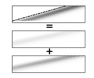
We can attempt to isolate these incompressible-like subsonic modes from the compressible effects in the flow by doing a Helmholtz decomposition of the velocity components $\hat {\boldsymbol {u}} = (\hat {u}, \hat {v}, \hat {w})$ of the leading resolvent mode $\boldsymbol {\psi }_1$. As described in § 2.5, the Helmholtz decomposition gives: (i) a solenoidal component $\hat {\boldsymbol {u}}^s$ and (ii) a dilatational component $\hat {\boldsymbol {u}}^d$ (in an incompressible flow, $\hat {\boldsymbol {u}}^d=0$). In figure 3, the full kinetic energy in figure 3($a$) is compared with the kinetic energy of $\hat {\boldsymbol {u}}^s$ in figure 3($b$) and of $\hat {\boldsymbol {u}}^d$ in figure 3($c$). The grey contour in figure 3($b$) is the same as that shown in figure 1($a$) and indicates the region of the wavenumber space where the incompressible resolvent is reasonably amplified.

Figure 3.

Kinetic energy of (a) the leading resolvent response $\boldsymbol {\psi }_1$ and of (b) the solenoidal and (c) the dilatational component of the velocity from $\boldsymbol {\psi }_1$ as a function of the streamwise and spanwise wavelengths ($\lambda _x, \lambda _z$) and a fixed phase speed $c = \bar {U}(y^+\approx 15)$. The grey contour line in panel (b) is the same as that shown in figure 1($a$) and shows the kinetic energy for the incompressible case at a third of the maximum.

The solenoidal response in figure 3($b$) looks similar to the response of the incompressible flow in figure 1($a$). Subsonic modes, i.e. the modes below the $\overline {Ma}(\infty )=1$ line, have solenoidal velocity, consistent with observations from DNS (Yu, Xu & Pirozzoli Reference Yu, Xu and Pirozzoli2019). Notably, in figure 3($b$), $\hat {\boldsymbol {u}}^s$ captures some of the energy in modes above the $\overline {Ma}(\infty )=1$ line where supersonic mechanisms are active. The grey contour line indicates that this occurs in the region where subsonic mechanisms are also active. These modes therefore have both the subsonic as well as supersonic mechanisms active. The co-existence of two amplification mechanisms provides an explanation for the observed decrease in the low-rank behaviour of these modes in figure 1($d$). However, the most interesting consequence of this co-existence of mechanisms is that it provides an additional route for amplifying the supersonic resolvent modes. This amplification route will be explained in § 5.2 and its potential importance to the real flow will be discussed in § 7.

3.2. Forcing to the subsonic modes: Helmholtz decomposition of resolvent forcing

In this section, we take the comparison between the compressible and incompressible operators one step further. For incompressible resolvent operators, if we consider Helmholtz decomposition of the forcing to the momentum equations $\hat {\boldsymbol {f}}_{\!\!\boldsymbol{u}}$, it is known that only the solenoidal component of the forcing $\hat {\boldsymbol{f}}_{\!\!\boldsymbol{u}}^s$ has any active influence in amplifying resolvent modes (Rosenberg & McKeon Reference Rosenberg and McKeon2019; Morra et al. Reference Morra, Nogueira, Cavalieri and Henningson2021). Although $\hat {\boldsymbol{f}}_{\!\!\boldsymbol{u}}^d$ is not zero in the real flow (i.e. the divergence of the full forcing $\boldsymbol {\nabla }\boldsymbol {\cdot } \hat {\boldsymbol{f}}_{\!\!\boldsymbol{u}} \neq 0$), this component cannot directly excite a response in velocity (Rosenberg & McKeon Reference Rosenberg and McKeon2019; Morra et al. Reference Morra, Nogueira, Cavalieri and Henningson2021). Here, we ask if this property of incompressible flows carries over to the subsonic modes of compressible flows. We will take $\hat {\boldsymbol{f}}_{\!\!\boldsymbol{u}}$ from the leading resolvent forcing mode $\boldsymbol {\phi }_1$ (the suboptimal modes are considered in Appendix A). A Helmholtz decomposition of this resolvent forcing mode gives the solenoidal component $\hat {\boldsymbol{f}}_{\!\!\boldsymbol{u}}^s = (\,\hat{f}^s_u, \hat {f}^s_v, \hat {f}^s_w)$ and the dilatational component $\hat {\boldsymbol{f}}_{\!\!\boldsymbol{u}}^d= (\,\hat {f}^d_u, \hat {f}^d_v, \hat {f}^d_w)$. We will consider the response to the solenoidal component alone through $\hat {\boldsymbol {f}}_{\!\!1}=(\,\hat {f}^s_u, \hat {f}^s_v, \hat {f}^s_w, 0, 0)$, and the response to the dilatational component along with the forcing to the density $\hat {f}_\rho$ and temperature $\hat {f}_\theta$ equations through $\hat {\boldsymbol {f}}_{\!\!2}=(\,\hat {f}^d_u, \hat {f}^d_v, \hat {f}^d_w, \hat {f}_\rho, \hat {f}_\theta )$. The response to $\hat {\boldsymbol {f}}_{\!\!1}$ is obtained as $\boldsymbol{\mathsf{H}} \hat {\boldsymbol {f}}_{\!\!1}$ and to $\hat {\boldsymbol {f}}_{\!\!2}$ as $\boldsymbol{\mathsf{H}} \hat {\boldsymbol {f}}_{\!\!2}$.

In figures 4($a$)–4($e$), for the same structure as in figure 2, the five components of the leading resolvent response mode in black is compared with the response to $\hat {\boldsymbol {f}}_{\!\!1}$ in blue and to $\hat {\boldsymbol {f}}_{\!\!2}$ in red. We see that the response is almost entirely captured by the solenoidal component of the forcing. To see that this is more generally true, in figure 4(f–j), the same comparison is shown for an $Re_\tau =450$ boundary layer with a higher Mach number of $Ma=6$, over a cooled wall with wall-cooling ratio $\varTheta _w/\varTheta _{ad}=0.25$. Here again, we see that the solenoidal component of the forcing captures a majority of the response. Therefore, like in the incompressible case, the subsonic resolvent modes are actively forced only by the solenoidal component of the forcing; and this is true both for flows over adiabatic and cooled walls.

Figure 4.

Response of the resolvent operator to the full leading resolvent forcing mode $\boldsymbol {\phi }_1$ (black) as well as the response to the two components of the forcing $\hat {\boldsymbol {f}}_{\!\!1}$ (blue) and $\hat {\boldsymbol {f}}_{\!\!2}$ (red). Subsonic modes with $(\lambda _x,\lambda _z,c)=(5,0.5,\bar {U}(y^+\approx 15))$ for two compressible boundary layers: (a–e) $Ma=4$, $Re_\tau =400$ over an adiabatic wall (the mode indicated by the ($\blacklozenge$) in figure 1$b$) and (f–j) $Ma=6$, $Re_\tau =450$ with $\varTheta _w/\varTheta _{ad}=0.25$. (a,f) Streamwise, (b,g) wall-normal and (c,h) spanwise velocities as well as the (d,i) density and (e,j) temperature.

4. Mach wave radiation from the resolvent operator

We will now focus on the region of the wavenumber space that falls above the $\overline {Ma}(\infty )=1$ line in figure 1($b$). The amplification in this region is largely due to supersonic resolvent modes. In this section, the connection between these resolvent modes and the relative Mach number defined in (3.1) is first established. We will then focus on the contribution of these modes to the free stream fluctuations of the boundary layer in § 4.1 and the effect of viscosity on these modes in § 4.2. Thereafter, from § 5 onward, we will concentrate on the forcing mechanisms that amplify these modes.

These supersonic modes above the $\overline {Ma}(\infty )=1$ line are pressure fluctuations that radiate into the free stream and they occur due to the Mach wave radiation mechanism as explained by Mack (Reference Mack1984). We will briefly follow the derivation of the Mach wave radiation by Mack (Reference Mack1984), with the difference of keeping the nonlinear terms as a forcing $\boldsymbol {f}$, rather than setting them to zero as done by Mack (Reference Mack1984). This will enable us to later isolate the two routes by which the Mach waves can cause high resolvent amplification: (i) the direct route (§ 5.1) and (ii) the indirect route (§ 5.2).

As done by Mack (Reference Mack1984), let us for simplicity consider the inviscid form of the governing equations Fourier transformed in $(x,y)$. As in (2.1), the nonlinear terms in the equations and any external disturbances to the flow are denoted as the unknown forcing $\hat {\boldsymbol {f}}$, therefore giving

(4.1a)\begin{gather} {\rm i}\bar{\rho} (k_x \bar{U}-\omega) \hat{u}_i ={-} \bar{\rho} \frac{{\rm d}\bar{U}}{{\rm d}y} \hat{v} \ \hat{\boldsymbol{i}} -\frac{1}{\gamma Ma^2} \frac{\partial}{\partial x_i} \hat{p} + \hat{f}_{u_i}, \end{gather}

(4.1b)\begin{gather}{\rm i}\bar{\rho} (k_x \bar{U}-\omega) \hat{\theta} = \bar{\varTheta} \frac{\partial \bar{\rho}}{\partial y} \hat{v} - (\gamma-1) \boldsymbol{\nabla}\boldsymbol{\cdot} \boldsymbol{u} + \hat{f}_\theta, \end{gather}

(4.1c)\begin{gather}{\rm i} \bar{\varTheta} (k_x \bar{U}-\omega) \hat{\rho} ={-} \bar{\varTheta} \frac{\partial \bar{\rho}}{\partial y} \hat{v} - \boldsymbol{\nabla}\boldsymbol{\cdot} \boldsymbol{u} + \hat{f}_\rho. \end{gather}

Here, $\boldsymbol {u}=(u_1,u_2,u_3)=(u,v,w)$ and we have used $\bar {\rho }\bar {\varTheta }=1$ to write $- \bar {\rho } \partial \bar {\varTheta }/\partial y = \bar {\varTheta } \partial \bar {\rho }/\partial y$. Pressure fluctuation $\hat {p}$ can be written using the linearised equation of state as $\hat {p} = \bar {\varTheta } \hat {\rho } + \bar {\rho } \hat {\theta }$. Using (4.1b) and (4.1c), and computing $\boldsymbol {\nabla }\boldsymbol {\cdot } \boldsymbol {u}$ from (4.1a), we rewrite this equation for $\hat {p}$ as

(4.2)\begin{align} -\frac{\partial^2 \hat{p}}{\partial y^2} + k^2(1-\overline{Ma}^2)\hat{p} & = {\rm i}\gamma Ma^2 \left[2 k_x \bar{\rho} \frac{{\rm d}\bar{U}}{{\rm d} y} + \frac{{\rm d}\bar{\rho}}{{\rm d}y} (k_x \bar{U}-\omega) \right] \hat{v} \nonumber\\ &\quad - \gamma Ma^2 \boldsymbol{\nabla}\boldsymbol{\cdot} \hat{\boldsymbol{f}}_{\!\!\boldsymbol{u}} + {\rm i}Ma^2 \bar{\rho} (k_x \bar{U}-\omega) \left( \hat{f}_\theta + \hat{f}_\rho \right) . \end{align}

Here, $k^2=k_x^2+k_z^2$ and $\hat {\boldsymbol{f}}_{\!\!\boldsymbol{u}} = (\,\hat {f}_u, \hat {f}_v, \hat {f}_w)$. (Please see Mack (Reference Mack1984) for a more complete derivation.) Note that in (4.2), $Ma$ denotes the free stream Mach number and $\overline {Ma}$ denotes the relative Mach number $\overline {Ma}(y)$ defined in (3.1). Following Mack (Reference Mack1984), let us consider the unforced equation within the free stream. In this case, the first term on the right-hand side of (4.2) is zero since the terms within the square brackets are zero in the free stream. The second and third terms are zero since we are considering the unforced equations. Therefore, the right-hand side of (4.2) goes to zero. For this equation, when $\overline {Ma}(y)>1$, we obtain a wave equation with solutions of the form

(4.3)\begin{equation} \hat{p}_M = {\rm i}\gamma {Ma}^2 \left(\frac{k_x\bar{U} - \omega}{k} \right) \exp{\left({-}k \left( 1-\overline{Ma}^2 \right)^{1/2} y\right)}. \end{equation}

These are the Mach waves of the flow derived by Mack (Reference Mack1984) as solutions of the inviscid unforced free stream equations when $\overline {Ma}(\infty )>1$. From (4.3), we get both upstream and downstream inclining waves, but only the downstream inclining waves satisfy the boundary conditions and therefore become valid solutions (Mack Reference Mack1984).

Going back to figure 1($b$), the supersonic resolvent modes are amplified only when $\overline {Ma}(\infty )\geqslant 1$ suggesting that these resolvent modes are Mach waves (Bae et al. Reference Bae, Dawson and McKeon2020b). To show that this is indeed the case, let us compare resolvent modes with (4.3). We pick the $(\lambda _x,\lambda _y)$ marked by a square ($\blacksquare$) in figure 1($b$) and the pressure $(\psi _1)_p$ from the leading resolvent mode of this structure is computed using the density $(\psi _1)_\rho$ and the temperature $(\psi _1)_\theta$ components as $(\psi _1)_p = \bar {\varTheta }(\psi _1)_\rho + \bar {\rho }(\psi _1)_\theta$. The real part of $(\psi _1)_p$ is shown as the red solid line in figure 5($a$). In the same figure, the real part of the Mach wave obtained using (4.3) is also shown in black (the amplitude and phase of the Mach wave is fixed to be the same as the resolvent mode at some arbitrary wall height, here $y=5$). To further compare, figure 5($b$) shows the negative (blue) and the positive (red) pressure fluctuations from the resolvent mode $(\psi _1)_p$ in a streamwise wall-normal ($x$–$y$) plane at a fixed spanwise location (here $z=0$). The black line-contours represent the Mach wave from (4.3) (the contours represent $\pm 0.5$ of the maximum value). From these figures, first we observe that, far from the wall, these resolvent modes are outgoing waves that radiate into the free stream. Additionally, we also note that, within the free stream, the resolvent modes closely follow the behaviour of the inviscid Mach wave. This further suggests that the Mach waves are responsible for the high resolvent amplification in the wavenumber region where the free stream relative Mach number is greater than $1$, i.e. $\overline {Ma}(\infty )\geqslant 1$. For the sake of completeness, the velocity, density and temperature components of this mode are also shown in figure 5($c$), and we see that these components also oscillate in the free stream.

Figure 5.

Leading resolvent response for the mode indicated by the square ($\blacksquare$) in figure 1(b). The mode corresponds to $\lambda _x=5$, $\lambda _z=3.5$ and $c=\bar {U}(y^+\approx 15)$ for a compressible boundary layer with $Ma=4$ and $Re_\tau = 400$ over an adiabatic wall. (a) Wall-normal profile of the real part of the pressure from the resolvent mode (red) compared with the pressure fluctuations from the inviscid Mach wave (black dashed) given by (4.3). (b) Pressure fluctuations in an $x\unicode{x2013}y$ plane with red (positive) and blue (negative) contours showing the real part of the pressure fluctuation from the resolvent mode and the black contour lines indicating the pressure fluctuations from the inviscid Mach wave at $\pm 0.5$ of the maximum. (c) Wall-normal profile of the streamwise (blue), wall-normal (green) and spanwise (orange) velocities, as well as the density (purple) and temperature (brown). The grey shaded regions indicate the boundary layer thickness.

So far, $\overline {Ma}(y)\geq 1$ just provides a condition for which we get modes that radiate into the free stream. The mechanism by which these modes cause high resolvent amplification is not obvious, and this will be discussed in § 5. Before that, we will briefly consider: (i) the contribution of these modes to the free stream disturbances of the boundary layer in § 4.1 and (ii) the impact of viscosity on these resolvent modes in § 4.2.

4.1. Contribution to the boundary layer and free stream

A crucial detail about these Mach waves is that, within the wavelength range considered here, these resolvent Mach waves are the the only modes that contribute to the response in the free stream. To illustrate this, in figure 6, the response to the masked resolvent is considered. The masking is done by introducing a weighting to the resolvent operator, as done by Nogueira et al. (Reference Nogueira, Cavalieri, Hanifi and Henningson2020) (see § 2.2). To obtain figure 6($a$), the resolvent is masked such that it gives a response only within the boundary layer, i.e. in the region $y \leqslant \delta _{99}$, and for figure 6($b$), the response is restricted to the free stream, i.e. $y > \delta _{99}$. First, from figure 6($a$), we observe that the subsonic modes lie within the boundary layer, consistent with the observations in § 3. The contribution to the free stream in figure 6($b$) then comes solely from the Mach wave resolvent modes. Therefore, the resolvent Mach waves are the only contributors to the free stream fluctuations from the resolvent, at least within the wavenumber space considered here.

Figure 6.

Masking of the resolvent operator to give a response (a) within the boundary layer (i.e. $y\leqslant d_{99}$) and (b) within the free stream (i.e. $y>d_{99}$), separately. The leading resolvent gain $\sigma _1$ from the masked operators is shown as a function of the streamwise and spanwise wavelengths $\lambda _x$ and $\lambda _z$ and for a fixed phase speed $c = \bar {U}(y^+\approx 15)$. The dashed black line represents the relative Mach equal to unity line.

4.2. Effect of viscosity on resolvent Mach wave amplification

From figure 1($b$), we see that the most linearly amplified supersonic modes are those that lie close to the $\overline {Ma}(\infty )=1$ line, and here we explore why this is the case. For the flows considered here, the maximum $\overline {Ma}(y)$ for the modes at the $\overline {Ma}(\infty )=1$ line is $1$ at $y=\delta _{99}$. Therefore, these modes have $\overline {Ma}(y)<1$ within the boundary layer, i.e. $\overline {Ma}(y<\delta _{99})<1$. Mach waves only start radiating from the wall height where $\overline {Ma}(y) \geqslant 1$. Hence, these modes near the $\overline {Ma}(\infty )=1$ line only start radiating at or near $y=\delta _{99}$, and they therefore do not have a presence within the boundary layer. These modes then exist in a region of the flow where the effect of viscosity is negligible. In contrast, supersonic modes that have $\overline {Ma}(\infty )>1$, i.e. fall much above the $\overline {Ma}(\infty )=1$ line, start radiating from within the boundary layer. These modes therefore experience the dampening effects of viscosity. This difference could explain why the most amplified supersonic modes lie close to the $\overline {Ma}(\infty )=1$ line.

To illustrate this, in figure 7, we compare the responses from the regular resolvent operator (black solid line) to fictional resolvent operators with viscosity artificially decreased to $1/10$ (red dash-dotted line) and $1/100$ (blue dash-dotted line) times the original value (note that these operators are not physical and are used here only for illustrative purposes). We saw in § 4.1 that only the Mach waves contribute to the free stream response from the resolvent. Therefore, to focus solely on the Mach waves, here, we ‘mask’ the resolvent such that the response from the resolvent is restricted to lie only in the free stream (see § 2.2). The vertical black dashed line represents $\overline {Ma}(\infty )=1$ and we are only interested in the region to the right of this line. First, let us address the jagged response from the regular resolvent. Although mathematically we can have Mach waves at a continuous range of temporal frequencies (4.3), because of our discretised operators, we only resolve a discrete set of these frequencies in our linear operator. The jagged response therefore comes about because of the proximity (or remoteness) of the selected $\omega$ to the nearest resolved frequency in the linear operator (Bae et al. Reference Bae, Dawson and McKeon2020b).

Figure 7.

Leading resolvent amplification for modes with $\lambda _x=1$ and $c \approx \bar {U}(y^+ = 15)$ as a function of $\lambda _z$. The solid line is obtained from the regular resolvent operator masked to give a response only within the free stream. The dashed lines are obtained from the fictional resolvent operators with viscosity artificially decreased to $1/10$ (red line) and $1/100$ (blue line) times the original value. The inset represents a zoomed-in version of the boxed region in the plot. The dashed line represents $\overline {Ma}(\infty )=1$.

From this figure, we see that the amplification of the mode at the $\overline {Ma}(\infty )=1$ line (see inset of the figure which zooms in on this mode) is not significantly affected by the reduction in viscosity. However, when $\overline {Ma}(\infty ) > 1$, reducing the dampening effect of viscosity results in more amplified modes. This suggests that the negligible effect of viscosity on the supersonic modes that lie at or close to the $\overline {Ma}(\infty )=1$ line is the reason why these modes are the most linearly amplified. These observations also suggests that, if in the future, the linearised equations augmented with an eddy-viscosity profile is used to study these free stream fluctuations (e.g. Del Álamo & Jiménez Reference Del Álamo and Jiménez2006; Pujals et al. Reference Pujals, García-Villalba, Cossu and Depardon2009; Hwang & Cossu Reference Hwang and Cossu2010), the amplification of modes with $\overline {Ma}(\infty ) > 1$ could potentially be impacted, although their mode shapes within the free stream will likely not be affected (since eddy viscosity in the free stream will be zero). However, analysing the eddy viscosity based operator is beyond the scope of the current manuscript and is left for the future.

5. Two routes of forcing resolvent Mach wave radiation

The $\overline {Ma}(y)\geq 1$ just provides a condition for which we get modes that radiate into the free stream. The mechanism by which these modes cause high resolvent amplification is not obvious. There are two routes, (i) direct and (ii) indirect, through which these Mach waves can cause high resolvent amplification, and here we will consider these two routes separately. In this section, two different supersonic resolvent modes from an $Ma=4$, $Re_\tau \approx 400$ turbulent boundary layer over an adiabatic wall are taken as examples: (i) ‘MW1 (Mach wave 1)’ with $\lambda _y=3.5$ in § 5.1 (the square $\blacksquare$ in figure 1$b$) and (ii) ‘MW2’ with $\lambda _y=10$ in § 5.2 (the circle ($\bullet$) in figure 1$b$). Both the modes have the same $\lambda _x=5$ and $c \approx \overline{U}(y^+=15)$. MW1 is chosen such that it falls close to the $\overline {Ma}(\infty )=1$ line, while MW2 is taken such that it lies further away from the $\overline {Ma}(\infty )=1$ line. This choice has two significant consequences. First, modes that lie close to the $\overline {Ma}(\infty )=1$ line have higher amplifications relative to other supersonic modes (see figure 1$b$ and § 4.2). Therefore, MW1 has a higher resolvent amplification when compared with MW2. Second, the Mach wave radiates only when $\overline {Ma}(y) \geqslant 1$. For MW1, the free stream relative Mach number $\overline {Ma}(\infty )$ (i.e. the maximum value of $\overline {Ma}(y)$) is close to $1$ and, therefore, the mode starts radiating from near $y=\delta _{99}$ (see § 4.2). However, MW2 has $\overline {Ma}(\infty )$ greater than $1$ and, therefore, the mode starts radiating from well within the boundary layer (see § 4.2). We will see that this difference impacts the forcing mechanisms active for these modes. In this section: (1) the ‘direct route’ of forcing the Mach waves will be discussed in § 5.1 using MW1 and (2) the ‘indirect route’ in § 5.2 using MW2. In § 6, we will look at the relative contributions of these two forcing routes across $(\lambda _x,\lambda _y,c)$.

5.1. Direct route of forcing resolvent Mach wave radiation

To probe the direct forcing route, consider the equations for the Mach waves (4.2) in the free stream. Consider the inverse of the resolvent operator $\boldsymbol{\mathsf{L}}=\boldsymbol{\mathsf{H}}^{-1}$, where $\boldsymbol{\mathsf{L}}\hat {\boldsymbol {q}}=\hat {\boldsymbol {f}}$, (2.5). The SVD of this operator gives $\boldsymbol{\mathsf{L}} = \sum _{i=1}^{5N} \boldsymbol{\phi}^{\boldsymbol{\prime}}_i \sigma '_i \boldsymbol {\psi}^{\boldsymbol{\prime}}_i$. For the inviscid case, solutions from (4.3) $\hat {p}_M(y)$ are solutions of $\boldsymbol{\mathsf{L}}$. Another way of saying this is that a singular vector of $\boldsymbol{\mathsf{L}}$, with a corresponding singular value of $\sigma '_i=0$, has pressure equal to $\hat {p}_M(y)$.

For the case of finite Reynolds numbers considered here, viscosity will damp these modes. Therefore, singular vectors with pressure $\hat {p}_M(y)$ will have singular values $\sigma '_i$ close to $0$, but not $0$. Let us now consider the SVD of the resolvent operator $\boldsymbol{\mathsf{H}}$ in terms of the SVD of $\boldsymbol{\mathsf{L}}=\boldsymbol{\mathsf{H}}^{-1}$. This gives $\boldsymbol{\mathsf{H}} = \sum _{i=1}^{5N} \boldsymbol {\psi}^{\boldsymbol{\prime}}_i (1/\sigma '_i) \boldsymbol {\phi}^{\boldsymbol{\prime}}_i$. There is $1/\sigma '_i$ that appears in the SVD of $\boldsymbol{\mathsf{H}}$. Therefore, singular vectors of $\boldsymbol{\mathsf{L}}$ with pressure $\hat {p}_M(y)$, which have $\sigma '_i$ close to $0$, will now appear as highly amplified singular vectors of $\boldsymbol{\mathsf{H}}$. This is how the Mach waves $\hat {p}_M(y)$ cause high resolvent amplification. Note that this mechanism can amplify $(\lambda _x,\lambda _y)$ modes that are linearly stable. In figure 1($b$), the green contour lines show the region of the $(\lambda _x,\lambda _y)$ space that is linearly unstable and we observe that there are supersonic modes outside of this region, i.e. that are linearly stable, but still have high resolvent amplification.

From (4.2), we see that, within the free stream, the pressure cannot be forced by $\hat {v}$ (since all the terms within the square brackets are zero in the free stream). Therefore, only $\boldsymbol {\nabla }\boldsymbol {\cdot }\hat {\boldsymbol{f}}_{\!\!\boldsymbol{u}}$, $\hat {f}_\theta$ or $\hat {f}_\rho$ can excite the waves. Now consider the Helmholtz decomposition of $\hat {\boldsymbol{f}}_{\!\!\boldsymbol{u}}$ that gives the solenoidal $\hat {\boldsymbol{f}}_{\!\!\boldsymbol{u}}^s$ and dilatational $\hat {\boldsymbol{f}}_{\!\!\boldsymbol{u}}^d$ components. Since, by the definition of the Helmholtz decomposition, $\boldsymbol {\nabla }\boldsymbol {\cdot } \hat {\boldsymbol{f}}_{\!\!\boldsymbol{u}}^s = 0$, only the dilatational component $\hat {\boldsymbol{f}}_{\!\!\boldsymbol{u}}^{d}$ can force these modes. To excite the Mach waves in the free stream, we therefore need a forcing in $\hat {\boldsymbol{f}}_{\!\!\boldsymbol{u}}^{d}$, $\hat {f}_\theta$ or $\hat {f}_\rho$.

To illustrate this, in figures 8($a$)–8($e$), we consider the supersonic mode MW1 (modes MW1 and MW2 are defined at the beginning of § 5). The five components of the full leading resolvent response $\boldsymbol {\psi }_1$ are shown in black (suboptimal modes are considered in Appendix A). The forcing $\hat {\boldsymbol {f}}$ to this resolvent mode is the leading resolvent forcing mode $\boldsymbol {\phi }_1$. In red is the response to $\hat {\boldsymbol{f}}_{\!\!\boldsymbol{u}}^d$, $\hat {f}_\rho$ and $\hat {f}_\theta$, i.e. the forcing to the resolvent is $\hat {\boldsymbol {f}}_{\!\!2}=(\,\hat {f}^d_u, \hat {f}^d_v, \hat {f}^d_w, \hat {f}_\rho, \hat {f}_\theta )$. In blue is the response to the remaining components of the forcing $\hat {\boldsymbol{f}}_{\!\!\boldsymbol{u}}^s$, i.e. the resolvent forcing is $\hat {\boldsymbol {f}}_{\!\!1}=(\,\hat {f}^s_u, \hat {f}^s_v, \hat {f}^s_w, 0, 0)$. From figures 8($a$)–8($e$), we see that $\hat {\boldsymbol {f}}_{\!\!2}$ is responsible for capturing the majority of the energy, and $\hat {\boldsymbol {f}}_{\!\!1}$ plays an insignificant role for these modes. (The reason for why the contribution of $\hat {\boldsymbol {f}}_{\!\!1}$ in figures 8$a$–8$e$, although small, is still non-zero, is explained in § 5.2.) Further, the contribution of $\hat {\boldsymbol{f}}_{\!\!\boldsymbol{u}}^d$ alone is shown in a lighter shade of green and that of ($f_\rho,f_\theta$) is shown in a darker shade of green. For the mode MW1, we note that both these components contribute almost equally to the response.

Figure 8.

Response of the resolvent operator to the full leading resolvent forcing mode $\hat {\boldsymbol {f}}=\boldsymbol {\phi }_1$ (black) as well as the response to the two components of the forcing $\hat {\boldsymbol {f}}_{\!\!1}$ (blue) and $\hat {\boldsymbol {f}}_{\!\!2}$ (red). Further, the contribution of $\hat {\boldsymbol{f}}_{\!\!\boldsymbol{u}}^d$ alone is shown in a lighter shade of green and that of ($f_\rho$,$f_\theta$) is shown in a darker shade of green. Two compressible boundary layers are considered: (a–e) $Ma=4$, $Re_\tau =400$ over an adiabatic wall and (f–j) $Ma=6$, $Re_\tau =450$ with $\varTheta _w/\varTheta _{ad}=0.25$. Modes that fall close to the relative Mach equal to unity lines are shown: mode $(\lambda _x,\lambda _z,c)=(5,3.5,\bar {U}(y^+\approx 15))$ for the $Ma=4$ case (the mode indicated by the square ($\blacksquare$) in figure 1$b$) and mode $(\lambda _x,\lambda _z,c)=(5,1.6,\bar {U}(y^+\approx 15))$ for the $Ma=6$ case. (a,f) Streamwise, (b,g) wall-normal and (c,h) spanwise velocities as well as the (d,i) density and (e,j) temperature.

To access the more general applicability of the discussions here, in figures 8($f$)–8($j$), we also look at a supersonic mode for an $Re_\tau =450$ boundary layer flow at a higher Mach number of $Ma=6$ and over a cooled wall with $\varTheta _w/\varTheta _{ad}=0.25$. Here again, we choose a mode that falls close to the relative Mach equal to unity line which for $c \approx \overline{U}(y^+=15)$ and $\lambda _x=5$ corresponds to $\lambda _z=1.6$. We observe similar trends as in figures 8($a$)–8($e$), where $\hat {\boldsymbol {f}}_{\!\!2}$ amplifies the mode. Therefore, wall cooling does not affect the trends discussed here.

5.2. Indirect route of forcing resolvent Mach wave radiation

So far, we considered mode MW1 and found that mainly the forcing components $\hat {\boldsymbol{f}}_{\!\!\boldsymbol{u}}^{d}$, $\hat {f}_\theta$ or $\hat {f}_\rho$ excite the mode. Let us now consider mode MW2 where this is not the case. Figure 9 is the equivalent of figures 8($a$)–8($e$), but for mode MW2. The five components of the full leading resolvent mode of MW2 is shown in black, along with the response to $\hat {\boldsymbol {f}}_{\!\!1}$ in blue and $\hat {\boldsymbol {f}}_{\!\!2}$ in red (the definitions of $\hat {\boldsymbol {f}}_{\!\!1}$ and $\hat {\boldsymbol {f}}_{\!\!2}$ are the same as in § 5.1). Unlike for MW1, for MW2, we find that $\hat {\boldsymbol {f}}_{\!\!1}$ (blue line), and therefore the solenoidal component of the forcing to the momentum equations, $\hat {\boldsymbol{f}}_{\!\!\boldsymbol{u}}^s$, plays a significant role in capturing the mode. The question then is, why does $\hat {\boldsymbol{f}}_{\!\!\boldsymbol{u}}^s$ excite MW2, but not MW1?

Figure 9.

Response of the resolvent operator to the full leading resolvent forcing mode $\hat {\boldsymbol {f}}=\boldsymbol {\phi }_1$ (black) as well as the response to the two components of the forcing $\hat {\boldsymbol {f}}_{\!\!1}$ (blue) and $\hat {\boldsymbol {f}}_{\!\!2}$ (red). Further, the contribution of $\hat {\boldsymbol{f}}_{\!\!\boldsymbol{u}}^d$ alone is shown in a lighter shade of green and that of ($f_\rho,f_\theta$) is shown in a darker shade of green. A supersonic mode with $(\lambda _x,\lambda _z,c)=(5,10,\bar {U}(y^+\approx 15))$ for a compressible boundary layer over an adiabatic wall with $Ma=4$, $Re_\tau =400$ is considered (the mode indicated by the circle ($\bullet$) in figure 1$b$). (a) Streamwise, (b) wall-normal and (c) spanwise velocities as well as the (d) density and (e) temperature.

To understand this, first, from (4.2), we note that wall-normal velocity $\hat {v}$ can excite the resolvent Mach waves. Second, from figure 1($b$), we note that both MW1 and MW2 lie within the grey contour line, which represents the region where incompressible mechanisms are reasonably active. Therefore, a possible route through which $\hat {\boldsymbol{f}}_{\!\!\boldsymbol{u}}^s$ can excite Mach waves is as follows: incompressible-like mechanisms cause $\hat {\boldsymbol{f}}_{\!\!\boldsymbol{u}}^s$ to excite a response in $\hat {v}$, which in turn excites the Mach waves. Here, we will call this the indirect route of forcing the Mach waves. However, this mechanism still does not explain the differences between the trends in the forcing to MW1 and MW2, specifically, why the indirect route is prominent for MW2 and not for MW1.

To probe this, in figure 10($a$), we consider MW1 and in figure 10($b$) we consider MW2. Two separate profiles are plotted in these figures. The first profile, $\hat {p}_M(y)$, is obtained from the analytic expression for the Mach wave radiation (4.3), and indicates the wall-normal region where these Mach waves exist. The red dashed line represents the wall height above which the relative Mach number $\overline {Ma}(y)\geqslant 1$ and, therefore, $\hat {p}_M(y)$ starts radiating only from this wall height. To compute the second profile, $(\psi ^{in}_1)_{v}(y)$, we consider a fictional incompressible resolvent operator $\boldsymbol{\mathsf{H}}^{in}$ (i.e. the resolvent operator at $Ma=0$), but with the mean velocity profile $\bar {U}$ from the compressible case. In effect, $\boldsymbol{\mathsf{H}}^{in}$ captures the mechanisms that would hypothetically be active in an $Ma=0$ flow that maintains the compressible mean velocity profile ($\boldsymbol{\mathsf{H}}^{in}$ is not physically relevant and is used here only for illustration). In other words, $\boldsymbol{\mathsf{H}}^{in}$ should be able to approximately capture the incompressible mechanisms in this flow. The profile $(\psi ^{in}_1)_{v}(y)$ is the wall-normal velocity component of the leading resolvent mode obtained from $\boldsymbol{\mathsf{H}}^{in}$. Finally, the red shaded region represents the overlap between $\hat {p}_M(y)$ and $(\psi ^{in}_1)_{v}(y)$ (in this region, $\overline {Ma}(y) \geqslant 1$ and, therefore, $\hat {p}_M(y)$ exists, and $(\psi ^{in}_1)_{v}(y)$ is at least $10\,\%$ of its maximum value). We see that, since MW2 starts radiating from well within the boundary layer, this region of overlap is significantly higher for the mode. The $\hat {v}$ generated through incompressible-like mechanisms forced by $\hat {\boldsymbol{f}}_{\!\!\boldsymbol{u}}^s$ can therefore much more efficiently drive the Mach waves in MW2, in comparison with MW1. This provides a possible explanation for why $\hat {\boldsymbol{f}}_{\!\!\boldsymbol{u}}^s$ plays a significant role in exciting MW2. The relatively small overlap observed in the case of MW1 also explains why the solenoidal component gives a small but non-zero response (blue line) in figures 8($a$)–8($e$).

Figure 10.

Analytical Mach wave $\hat {p}_M(y)$ in (4.2) and $(\psi ^{in}_1)_{v}(y)$ the wall-normal velocity obtained from the incompressible resolvent with the compressible mean $\boldsymbol{\mathsf{H}}^{in}$ for the modes (a) MW1 and (b) MW2. The grey shaded region represents the region within the boundary layer. The red shaded region represents the overlap between $\hat {p}_M(y)$ and $(\psi ^{in}_1)_{v}(y)$, where $\overline {Ma}(y) \geqslant 1$ and therefore $\hat {p}_M(y)$ exists, and $(\psi ^{in}_1)_{v}(y)$ is at least $10\,\%$ of its maximum value.

From this, we see that there are two factors that are responsible for this indirect forcing. (1) The modes should have active incompressible-like mechanisms. This is true for both MW1 and MW2, and can be measured by the leading singular value of $\boldsymbol{\mathsf{H}}^{in}$, $\sigma ^{in}_{1}(\lambda _x,\lambda _y,c)$. (2) There should be an overlap between $\hat {p}_M(y)$ and $(\psi ^{in}_1)_{v}(y)$. This is more significant for MW2 and can be measured using a projection of $(\psi ^{in}_1)_{v}$ onto $\hat {p}_M(y)$ defined as

(5.1)\begin{equation} \eta(\lambda_x,\lambda_y,c) = \frac{ \left( \displaystyle\int\nolimits_0^{y_{f}}\hat{p}_M(y) (\psi^{in}_1)_{v}^*(y) \right)^2}{ \displaystyle\int\nolimits_0^{y_{f}} \hat{p}_M(y) \hat{p}_M^*(y) \displaystyle\int\nolimits_0^{y_{f}} (\psi^{in}_1)_{v}(y) (\psi^{in}_1)_{v}^*(y) }. \end{equation}

Therefore, if this mechanism is indeed responsible for amplification, then the mode should have a higher value of $(\sigma ^{in}_{1})^2 \eta$. The wall height $y_f$ is the height until which we force the resolvent and here, $y_f=3$ (see § 2.4). The value of $(\sigma ^{in}_{1})^2 \eta$ is approximately $102$ for MW1 and $202$ for MW2, showing that the indirect route is more active for MW2 (although computing this number shows that this route is not completely absent for MW1, but just less significant). We will use this metric $(\sigma ^{in}_{1})^2 \eta$ in § 6.

6. Contribution of the direct and indirect forcing mechanisms

So far, we have considered a decomposition of the forcing to the resolvent into two components: (1) $\hat {\boldsymbol {f}}_{\!\!1}=(\,\hat {f}^s_u, \hat {f}^s_v, \hat {f}^s_w, 0, 0)$, which contains the solenoidal component of the forcing to the momentum equations; and (2) $\hat {\boldsymbol {f}}_{\!\!2}=(\,\hat {f}^d_u, \hat {f}^d_v, \hat {f}^d_w, \hat {f}_\rho, \hat {f}_\theta )$, which contains the dilatational component of the forcing to the momentum equations as well as the forcing to the density and temperature equations. Subsonic modes are forced by $\hat {\boldsymbol {f}}_{\!\!1}$. However, there are two routes through which the supersonic modes can be forced: the direct route, where $\hat {\boldsymbol {f}}_{\!\!2}$ is active, and the indirect route, where $\hat {\boldsymbol {f}}_{\!\!1}$ plays a significant role. So far, we have only looked at individual $(\lambda _x,\lambda _y,c)$ modes and the purpose of this section is to analyse the relative importance of $\hat {\boldsymbol {f}}_{\!\!1}$ and $\hat {\boldsymbol {f}}_{\!\!2}$ over a range of $(\lambda _x, \lambda _y,c)$.

In figure 11, for the case of a turbulent boundary layer at $Ma=4$ and $Re_\tau =400$, the full resolvent response in figure 11(a,d) is compared with responses to $\hat {\boldsymbol {f}}_{\!\!1}$ in figure 11(b,e) and $\hat {\boldsymbol {f}}_{\!\!2}$ in figure 11(c,f). Figure 11(a–c) shows the responses as a function of ($\lambda _x,\lambda _z$) at a fixed phase speed of $c=\overline{U}(y^+\approx 15)$. To consider a range of $c$, figure 11(d–f) shows the responses as a function of $c$ and $\lambda _z$, at a fixed value of $\lambda _x=5$. (The values of $c$ in figures 11($d$)–11($f$) are taken only until $0.75$, since the amplification of the subsonic streaks with $c>0.75$ is too high to be clearly depicted along with the lesser amplified supersonic modes.) The black contour lines represent $-1:1:2$ contours of $\log _{10}((\sigma ^{in}_{1})^2 \eta )$ which, as seen in § 5.2, indicate the region where (i) incompressible-like mechanisms are active and (ii) $(\psi ^{in}_1)_{v}$ projects onto $\hat {p}_M(y)$ (see § 5.2). The black dashed lines in the figures (or curves in the case of figure 11d–f) indicates relative Mach number equal to unity $\overline {Ma}(\infty )=1$. Note that the colour scales in this figure are logarithmic.

Figure 11.

Chu norm of the response of the resolvent operator to (a,d) the full leading resolvent forcing mode $\boldsymbol {\phi }_1$ as well as the two components of the forcing (b,e) $\hat {\boldsymbol {f}}_{\!\!1}$ and (c,f) $\hat {\boldsymbol {f}}_{\!\!2}$ in two ways: (a–c) as a function of the streamwise and spanwise wavelengths $(\lambda _x,\lambda _z)$ at a fixed phase speed $c=\bar {U}(y^+\approx 15)$ and (d–f) as a function of phase speeds and spanwise wavelengths ($c,\lambda _z$) at a fixed streamwise wavelength $\lambda _x=5$. The vertical dash-dotted line in panel (a) indicates $\lambda _x=5$ and in panel (d), indicates $c=\bar {U}(y^+\approx 15)$. The solid black contours in panel (b) indicate $-1:1:2$ contours of $\log _{10}((\sigma ^{in}_{1})^2 \eta )$. The dashed black contour lines indicate the relative Mach equal to unity.

From figures 11($b$) and 11($e$), we observe that $\hat {\boldsymbol {f}}_{\!\!1}$ captures the responses in the subsonic modes, i.e. the responses in the region below the $\overline {Ma}(\infty )=1$ line. Figures 11($c$) and 11($f$) show that $\hat {\boldsymbol {f}}_{\!\!2}$ captures the majority of the response in the supersonic modes, i.e. the responses in the region above the $\overline {Ma}(\infty )=1$ line. This is especially true when considering the most amplified supersonic modes that are near the $\overline {Ma}(\infty )=1$ line, consistent with observations in § 5. Also in line with § 5, from figures 11($b$) and 11($e$), we note that there is a small set of supersonic modes where the contribution of $\hat {\boldsymbol {f}}_{\!\!1}$ is not zero. The black contour lines in figure 11($b$) follow the trends of these modes, which suggests that an incompressible-like mechanism is active, and this mechanism can force the Mach waves. Therefore, the indirect route of forcing (§ 5.2) is active for these modes.

In figure 12, we consider an $Ma=6$, $Re_\tau =450$ turbulent boundary layer over a cooled wall with wall-cooling ratio $\varTheta _w/\varTheta _{ad}=0.25$, with figures 12($a$), 12($b$) and 12($c$) showing responses to the full forcing, to $\hat {\boldsymbol {f}}_{\!\!1}$ and to $\hat {\boldsymbol {f}}_{\!\!2}$, respectively. We observe that the same trends as observed for the $Ma=4$ boundary layer is valid here, indicating that wall cooling does not impact the trends discussed. These discussions are also equally valid for laminar compressible boundary layers, and Appendix C briefly discusses this case. Another point to note is that we have so far only discussed the most amplified first resolvent mode, and Appendix A contains a brief discussion on the effect of the different components of the forcing on the sub-optimal resolvent modes.

Figure 12.

For a turbulent boundary layer with $Ma=6$, $Re_\tau =450$ and $\varTheta _w/\varTheta _{ad}=0.25$, the Chu norm of the response of the resolvent operator to (a) the full leading resolvent forcing mode $\boldsymbol {\phi }_1$ as well as the two components of the forcing (b) $\hat {\boldsymbol {f}}_{\!\!1}$ and (c) $\hat {\boldsymbol {f}}_{\!\!2}$ as a function of the streamwise ($\lambda _x$) and spanwise ($\lambda _z$) wavelengths for a fixed value of phase speed $c=\bar {U}(y^+\approx 15)$. The dashed lines indicate the relative Mach number equal to unity.

From these observations, we see that within the majority of the wavenumber space above the $\overline {Ma}(\infty )=1$ line, the contribution of $\hat {\boldsymbol {f}}_{\!\!2}$ is orders of magnitude higher than the contribution of $\hat {\boldsymbol {f}}_{\!\!1}$ (given that the colour scale is logarithmic). This is especially true for the most amplified resolvent modes that lie close to the $\overline {Ma}(\infty )=1$ line. However, this does not mean that the contribution of $\hat {\boldsymbol {f}}_{\!\!1}$ is not significant for supersonic modes. In the next section, we will discuss a comparison with DNS, where $\hat {\boldsymbol {f}}_{\!\!1}$ can be seen to play a dominant role in exciting the supersonic modes of the flow.

7. Resolvent Mach waves and Mach waves from DNS: a discussion

In this section, we will discuss the resolvent Mach waves alongside trends of these waves that are known from DNS (e.g. Duan et al. Reference Duan, Choudhari and Wu2014, Reference Duan, Choudhari and Zhang2016; Zhang et al. Reference Zhang, Duan and Choudhari2017). The turbulence within the boundary layer forces Mach wave radiation. DNS studies show that with increasing $Ma$, the free stream inclination angles of these Mach waves decrease and their propagation velocities increase (Duan et al. Reference Duan, Choudhari and Zhang2016). However, increasing wall cooling does not seem to impact propagation speeds of the waves, but the inclination angles are reported to be slightly steeper (Zhang et al. Reference Zhang, Duan and Choudhari2017). Crucially, these studies employed acoustic analogy based arguments, and identified the sources of these waves to lie within the buffer layer of the flow.

To analyse these Mach waves that are radiated by the buffer layer, we have to move away from using resolvent analysis over the entire wall-normal domain, as has been done in previous works (e.g. Bugeat et al. Reference Bugeat, Chassaing, Robinet and Sagaut2019; Bae et al. Reference Bae, Dawson and McKeon2020b). We will instead use the ‘masked resolvent’, where the forcing and the response to the resolvent is masked, i.e. restricted to lie in particular wall-normal regions of the flow. First, considering the response, Mach wave responses alone are of interest here and we have observed that these Mach waves are the sole contributors to the free stream resolvent response (see § 4.1). Therefore, the resolvent response can be masked such that it lies within the free stream alone. Next, considering the forcing, DNS studies have shown that the sources to these waves lie within the buffer layer of the flow (e.g. Duan et al. Reference Duan, Choudhari and Wu2014, Reference Duan, Choudhari and Zhang2016; Zhang et al. Reference Zhang, Duan and Choudhari2017). Therefore, the resolvent forcing can be masked such that it is localised within the buffer layer. So we are here considering the resolvent operator such that its forcing can only lie within $y^+<30$ and the response within $y>\delta _{99}$. The weighting function introduced by Nogueira et al. (Reference Nogueira, Cavalieri, Hanifi and Henningson2020) is used to mask the resolvent (see § 2.2).

Figure 13 shows the response to such a masked resolvent, with figures 13($a$), 13($b$) and 13($c$) showing the response to the full forcing, to $\hat {\boldsymbol {f}}_{\!\!1}$ and to $\hat {\boldsymbol {f}}_{\!\!2}$, respectively. Here, $c=\bar {U}(y^+\approx 15)$ is taken from within the buffer layer. Comparing figure 13($a$) with figure 11($b$), the response of the masked resolvent is concentrated in the region where we found that the indirect route of forcing is significant. Additionally, from figures 13($b$) and 13($c$), we see that $\hat {\boldsymbol {f}}_{\!\!1}$ captures almost all of the response. Therefore, based on the discussions in § 6, we can postulate that the indirect route of forcing amplifies these modes. Purely from a resolvent perspective, we can therefore hypothesise that the Mach wave radiation due to the turbulence within the buffer layer of the boundary layer is generated due to the indirect route of forcing as described in § 5.2.

Figure 13.

Response of the masked resolvent; the response is masked to lie solely within the free stream and the forcing to lie within $y^+<30$. The Chu norm of the response of the resolvent operator to (a) the full leading resolvent forcing mode $\boldsymbol {\phi }_1$ as well as the two components of the forcing (b) $\hat {\boldsymbol {f}}_{\!\!1}$ and (c) $\hat {\boldsymbol {f}}_{\!\!2}$ as a function of the streamwise ($\lambda _x$) and spanwise ($\lambda _z$) wavelengths for a fixed value of phase speed $c \approx \bar {U}(y^+=15)$. The $Ma=4$, $Re_\tau =400$ turbulent boundary layer over an adiabatic wall is considered. The dashed black line indicates the relative Mach number equal to unity line.

Presuming the accuracy of this hypothesis, both the indirect route of Mach wave forcing and the subsonic modes are forced by the solenoidal component of the forcing. This could potentially reduce the problem of modelling the full high-rank nonlinear forcing in these flows to the simpler problem of modelling only the lower-rank solenoidal component of the forcing.

7.1. Inclination angle of the supersonic resolvent modes

DNS studies have investigated the free stream inclination angles of the Mach wave radiation generated from the boundary layer (e.g. Duan et al. Reference Duan, Choudhari and Wu2014; Zhang et al. Reference Zhang, Duan and Choudhari2017). Although DNS datasets show some degree of variability in the free stream inclination angles observed, these studies consistently emphasise the existence of a statistically dominant angle. When considering the Mach waves from the resolvent model, we can use the fact that these waves are pressure oscillations of the form given by (4.3) and compute the free stream inclination angle of these Mach waves as

(7.1)\begin{equation} \angle_{FS} = \tan^{{-}1} \left( \frac{-1j}{\sqrt{1+(\lambda_x/\lambda_z)^2-{Ma}^2 (1-c)^2}} \right). \end{equation}

At a fixed Mach number, we see that the inclination angle depends on the aspect ratio $\lambda _x/\lambda _z$ and the phase speed $c$ of the mode. From the resolvent, we therefore have a range of inclination angles. The mechanism that picks out the statistically dominant inclination angles found in DNS is still not clear. To probe into this mechanism, in the future, there is a requirement of comparing DNS data with the resolvent model. More specifically, constructing a resolvent-based low-order model of the free stream radiations using DNS data from the buffer layer alone will potentially elucidate the mechanism that is responsible for the selection of a predominant angle in DNS studies. This detailed comparison with DNS, however, is beyond the scope of the current manuscript, and is left as an important future direction of work.

Although we cannot do a one-to-one comparison with DNS, we can still compare some of the trends observed in DNS with that from the resolvent model. For this, in figure 14, the solid lines show the inclination angles of the resolvent free stream radiation computed from (7.1) as a function of Mach number for a range of aspect ratios and phase speeds. The phase speed increases in the direction of the arrow in figure 14 and, for each phase speed, lighter coloured lines represent larger aspect ratios. First, we observe that phase speeds have a more prominent impact on the free stream inclination angles, when compared with aspect ratios. Second, from (7.1), we observe that wall cooling does not have a direct impact on the inclination angles of the structures. It only has an indirect effect through a control on the values of $c$ that can be admitted for these waves (through the differences in mean profiles due to wall cooling). Finally, we note that, in general, the inclination angles obtained from the model decrease with increasing Mach number, and this trend is consistent with DNS (Duan et al. Reference Duan, Choudhari and Wu2014).

Figure 14.

Inclination angle of the inviscid Mach waves given by (7.1) with respect to Mach number for a range of aspect ratios and phase speeds. Three different phase speeds of $c=0.3$, $0.5$ and $0.7$ increasing in the direction of the arrow and three different values of aspect ratios $\lambda _x/\lambda _z=0$, $0.5$ and $1.0$ are considered. The markers indicate the average inclination angles of the Mach waves from DNS reported in the literature (Duan et al. Reference Duan, Choudhari and Wu2014; Zhang et al. Reference Zhang, Duan and Choudhari2017). The DNS data at $Ma=6$ are for the case of cooled walls, and the two markers indicate two different ratios of $\varTheta _w/\varTheta _{ad}=0.76$ (blue) and $0.25$ (red). The intervals represent the range of inclination angles predicted by the resolvent model under two assumptions: (1) $k_z=0$ and (2) $\bar {U}(y^+ = 10) \leqslant c \leqslant \bar {U}(y^+ = 20)$.

The markers show the values of the average free stream inclination angles that are obtained from DNS (Duan et al. Reference Duan, Choudhari and Wu2014; Zhang et al. Reference Zhang, Duan and Choudhari2017) from an $Ma=2.5$ flow over an adiabatic wall, and an $Ma=6$ flow with two wall-cooling ratios of $\varTheta _w/\varTheta _{ad}=0.76$ and $0.25$ (indicated by the two markers at $Ma=6$). The intervals plotted show the range of inclination angles predicted by the resolvent under two assumptions: (1) the phase speed lies within the buffer layer $\bar {U}(y^+ \approx 10) \leqslant c \leqslant \bar {U}(y^+ \approx 20)$ and (2) the aspect ratio is zero, since from figure 13, the most amplified resolvent modes that can be forced from the buffer layer tend to have large $\lambda _z$ (also see Bugeat et al. Reference Bugeat, Chassaing, Robinet and Sagaut2019). It could be argued that when the effect of wall cooling is not significant (green and blue markers), the average inclination angles obtained from DNS fall roughly within the range of inclination angles that are observed from the model. However, there are major discrepancies. First, the range of inclination angles predicted for $Ma=2.5$ is too large for any meaningful comparison to be made. Second, DNS predicts an increase in the inclination angle with increasing wall cooling, while resolvent predicts the opposite trend, i.e. a decrease in the inclination angle.

These differences could be due to several reasons and some of them are: (1) the assumption of phase speeds and aspect ratios that we have considered for plotting the intervals are oversimplified; or (2) the rank-1 resolvent model that we have used here is not sufficient. However, the most obvious restriction in comparing the inclination angles, as done here, is the assumption that all $(k_x,k_z,c)$ modes are forced equally. This cannot be true, since the dominant turbulent structures within the boundary layer will determine the extent to which these modes are forced. These turbulent structures can also be impacted by wall cooling, thereby influencing the dominant angles of these radiations. To address this, there is again the need to construct resolvent-based low-rank models of the free stream, and this is an important future direction of work.

8. Mach wave radiation from a streamwise developing boundary layer

The aim of this section is to briefly show that the mechanisms generating the Mach wave radiations, as discussed here, can be generalised to a streamwise developing boundary layer. In this case, the mean velocity is a function of the streamwise and wall-normal directions $\bar {U}(x,y)$. Unlike in the case of the one-dimensional (1-D) boundary layer, for the growing boundary layer, the wall-normal mean velocity $\bar {V}(x,y)$ is not zero. Without the simplifying assumptions for the 1-D boundary layer, the inviscid equations for pressure in (4.2) will now become

(8.1)\begin{align} &\omega^2p - 2\omega\bar{U}_i \frac{\partial p}{\partial x_i} + \bar{U}_i\bar{U}_j \frac{\partial p}{\partial x_i \partial x_j} + \bar{U}_i \frac{\partial \bar{U}_j }{\partial x_i}\frac{\partial p}{\partial x_j} + \gamma \omega \frac{\partial \bar{U}_j }{\partial x_j} p +\gamma \bar{U}_i \frac{\partial \bar{U}_j }{\partial x_j} \frac{\partial p}{\partial x_i} \nonumber\\ &\quad - \gamma \frac{\partial \bar{U}_i }{\partial x_j}\frac{\partial \bar{U}_j }{\partial x_i} p - \frac{1}{M^2} \frac{\partial \bar{\varTheta} }{\partial x_j} \frac{\partial p}{\partial x_j} - \frac{\bar{\varTheta}}{M^2} \frac{\partial^2 p}{\partial x_j^2}= \gamma \left[ 2\frac{\partial \bar{U}_i}{\partial x_j} \frac{\partial }{\partial x_i} +\frac{\partial^2 \bar{U}_i }{\partial x_i\partial x_j} \right] u_j\nonumber\\ &\quad + \left[ \omega +\bar{U}_i \frac{\partial }{\partial x_i}\right] \left( \bar{\varTheta}f_\rho+f_\theta \right) - \gamma \frac{\partial f_{u_i}}{\partial x_i}. \end{align}

Here, $(x_1,x_2,x_3)=(x,y,z)$, $(u_1,u_2,u_3)=(u,v,w)$, $(\bar {U}_1,\bar {U}_2,\bar {U}_3)=(\bar {U},\bar {V},0)$ and $(f_{u_1},f_{u_2},f_{u_3})=(f_x,f_y,f_z)$. A Fourier transform is taken in the homogeneous spanwise direction $z$. Within the free stream, the left-hand side of (8.1) can be solved using separation of variables to obtain solutions of the form (Mack Reference Mack1990)

(8.2)\begin{equation} p(x,y)=A\exp(r_xx)\exp(r_yx). \end{equation}

Here, $A$ is a constant at $(k_z,\omega )$, and $r_x$ and $r_y$ can be obtained by solving the ordinary differential equations obtained from the separation of variables. These wavenumbers follow one of these two sets of quadratic equations: (i) $c_1 r_x^2 - c_3r_x - l_1 = 0$ and $c_2 r_y^2 + (c_5 r_x - c_4) r_y + (l_1 + c_6) = 0$ or (ii) $c_2 r_y^2 - c_4r_y - l_2 = 0$ and $c_1 r_x^2 + (c_5 r_y - c_3) r_x + (l_2 + c_6) = 0$. The constants depend on the mean free stream quantities alone as $c_1 = (1 - 1/M^2)$, $c_2 = (\bar {V}_\infty ^2 - 1/M^2)$, $c_3 = 2\omega$, $c_4 = 2\omega \bar {V}_\infty$, $c_5 = 2\bar {V}_\infty$ and $c_6 = (\omega ^2 - k_z^2/M^2 )$, where $\bar {V}_\infty$ represents the free stream wall-normal velocity normalised by $U_\infty$. By varying the constant $l_1$ (or $l_2$), we can get a family of solutions at a range of $(r_x,r_y)$. Therefore, for the streamwise developing boundary layer, we can obtain wave-like solutions within the free stream, consistent with the observations for the 1-D case in the rest of the manuscript (Mack Reference Mack1990).

Now considering the right-hand side of (8.1) and comparing it with the 1-D boundary layer (4.2), we can obtain similar observations. There are two routes of forcing. First, the dilatational part of the forcing to the momentum equations $\hat {\boldsymbol {f}}_d$ (obtained through $\partial f_{u_i}/\partial x_i$), along with the forcing to the continuity $f_\rho$ and energy $f_\theta$ equations, can directly force the pressure waves. This gives the direct route of forcing as in § 5.1. Second, the solenoidal component of the forcing can generate a response in velocity $u_j$, which in turn can force the pressure equations within the boundary layer. (Although $u_j$ cannot be assumed to be zero in the free stream, the terms within the square brackets that multiply with $u_j$ can be assumed to be zero in this region.) This gives us the indirect route of forcing as in § 5.2. Consistent with prior observations from the 1-D case, the indirect route of forcing involves the mean shear profiles and can therefore be expected to be dominant in the buffer layer where this mean shear is high.

As done in § 4, to confirm if these conclusions derived from the inviscid solutions do indeed capture features of the resolvent at a finite Reynolds number, figure 15 shows a 2-D resolvent mode. To obtain the 2-D resolvent mode, the linearised discrete Navier–Stokes equations contained in the matrix $\boldsymbol {A}$ in (2.3) are now constructed using the 2-D mean profiles $\bar {U}(x,y)$ and $\bar {V}(x,y)$ obtained from Duan et al. (Reference Duan, Choudhari and Zhang2016). The derivatives are now $(\partial /\partial x,\partial /\partial y,\partial /\partial z)=(\partial /\partial x,\partial /\partial y, i k_z)$. The boundary conditions in the free stream are the same as for the 1-D resolvent (see § 2.4). The inlet and outlet boundary conditions are the non-reflecting Navier–Stokes characteristic boundary conditions (Poinsot & Lele Reference Poinsot and Lele1992) with damping sponges to prevent any reflections (Freund Reference Freund1997). For the 2-D resolvent, at a particular value of $(k_z,\omega )$, we obtain a range of modes at different $k_x$ that includes both subsonic and supersonic modes. To obtain just the Mach wave radiation that is of interest here, we will therefore consider the resolvent with the response masked such that it lies only in the free stream.

Figure 15.

Leading resolvent response mode obtained from the 2-D resolvent analysis for spanwise wavenumber $k_z=12.62$ and temporal frequency $\omega =3.15$. (a,d) Full response, with the resolvent masked such that the response is solely in the free stream. Also shown are the responses to the forcing (b,e) $\hat {\boldsymbol {f}}_{\!\!1}$ and (c,f) $\hat {\boldsymbol {f}}_{\!\!2}$. The modes obtained from two different masking for the forcing are shown: (a–c) the forcing lies throughout the boundary layer and part of the free stream, here until $y\leq 3$, and (d–f) the forcing lies within the buffer layer, $y^+\leq 30$. Note, for clarity, only the free stream and a subset of the streamwise domain used to compute the resolvent is shown here. The approximate streamwise wavenumber $k_x$ and phase speed $c$ obtained using a Fourier transform of the mode, are also shown. The contour lines in panels (a,d) show the analytical solution obtained by solving the inviscid pressure equations in the free stream, with red and blue contour lines representing positive and negative pressure fluctuations, respectively.

Figures 15($a$) and 15($d$) show the pressure obtained from the 2-D resolvent mode as the filled contours. Note, for clarity, only the free stream and a subset of the streamwise domain used to compute the resolvent is shown in the figure. The line contours represent the solution to the inviscid free stream pressure equation (8.2). The constant for the quadratic equation $l_1$ (or $l_2$) is fixed such that $r_x$ (or $r_y$) matches the streamwise (or wall-normal) wavenumber of the resolvent mode in the free stream, which is obtained from a Fourier transform. Here, red and blue represent positive and negative fluctuations, respectively. An $Ma=5.86$, $T_w/T_{ad}\approx 0.76, T_\infty = 55\ {\rm K}$ boundary layer is considered here. A temporal frequency $\omega =3.15$ is chosen, since, from DNS, we know that this frequency is energetic in the free stream (Duan et al. Reference Duan, Choudhari and Zhang2016), and a spanwise wavenumber of $k_z=12.62$ is chosen. The dash-dotted line represents the Mach angle computed as $\sin ^{-1}{(1/Ma)}$. Unlike in the 1-D resolvent, due to the finite nature of the domain, the forcing is restricted to a finite streamwise extent and, therefore, the radiation from the resulting response modes will be restricted by the Mach angle (note, as seen in the figure, the inclination angle of the mode can be different from this Mach angle). The forcing and response are not masked in the streamwise direction. Two options for masking the forcing in the wall-normal direction are used: (i) in figures 15($a$)–15($c$), the forcing is allowed to lie anywhere within the boundary layer or part of the free stream, i.e. at $y\leq 3$; and (ii) in figures 15($d$)–15($f$), the forcing lies exclusively within the buffer layer of the flow, i.e. $y^+\leqslant 30$. The response to the forcing $\hat {\boldsymbol {f}}_{\!\!1}$ is shown in figures 15($b$) and 15($e$), and to $\hat {\boldsymbol {f}}_{\!\!2}$ in figures 15($c$) and 15($f$).

First, from figures 15($a$) and 15($d$), we see that the inviscid equations do match the resolvent modes reasonably well. This shows that, like we observed for the 1-D resolvent, the 2-D resolvent also admits wave-like solutions in the free stream, which can be analytically modelled as solutions to the inviscid free stream equations. Second, comparing figures 15($b$) and 15($c$), we see that when the forcing is allowed reach to $y=3$, $\hat {\boldsymbol {f}}_{\!\!2}$ contributes dominantly to the mode. In other words, in this case, through the direct route, the dilatational component of the forcing to the momentum equations, and the forcing to the energy and continuity equations force the mode. However, from figures 15($e$) and 15($f$), we see that this observation is no longer true when the forcing is within the buffer layer alone. In this case, through the indirect route, the solenoidal component of the forcing to the momentum equations $\hat {\boldsymbol {f}}_{\!\!1}$ dominates the response.

Therefore, similar to the 1-D resolvent, there are two routes through which the Mach waves in the 2-D resolvent can be forced: (i) the direct and (ii) the indirect route. The indirect route likely becomes more important when considering modes forced by the buffer layer of the flow. This is consistent with the results obtained from the 1-D resolvent, and therefore shows that, in this case, the conclusions drawn here from the 1-D resolvent analysis are valid for the trends from the 2-D resolvent. Also consistent with the 1-D resolvent, by varying $k_z$, we can obtain modes (at a range of $k_x$) with different ratios of the solenoidal to the dilatational responses (not shown here for brevity). It would be interesting, in the future, to understand how the pressure radiations obtained in (8.2) may relate to mechanisms where the spatial modulation of wavepackets leads to radiation (e.g. Reba, Narayanan & Colonius Reference Reba, Narayanan and Colonius2010; Jordan & Colonius Reference Jordan and Colonius2013). A detailed analysis of the 2-D resolvent is therefore important and is a crucial future direction of work.