


1. Introduction
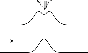
A uniform free-surface flow will remain flat unless there is a disturbance in its path. Some alteration in the topography over which the flow moves, or some pressure acting on the surface, neither of which are necessarily observed easily, will cause deformation of the free surface. Although there are certainly more ways to disturb the fluid flow (e.g. plate or sluice gate), for this paper we will focus solely on the topographical features or pressure distributions acting as the forcing on the flow – specifically, in understanding the relationship between the form of the surface and the disturbances. We also consider only steady free-surface flows for which the surface holds a constant shape, removing any time dependence from the problem.
Approaches can be split into two categories. It can be asked what the response of the free surface would be to a particular form of forcing, how adding or removing material on the topography or applying a particular pressure to the surface will change the surface profile; this is known as the forwards problem. In contrast, it might instead be asked for a given free surface, what were the causative disturbances to the flow that produced that profile; this is known as the inverse problem.
The forwards problem has seen much attention. In two dimensions, the introduction of the complex potential and some further mappings allows the problem to be cast as a boundary integral equation. Forbes & Schwartz (Reference Forbes and Schwartz1982) and Vanden-Broeck (Reference Vanden-Broeck1987) used these methods to compute solutions to free-surface flow past semicircular topography. This has been extended to consider more complicated topographies (see e.g. the work of Binder, Vanden-Broeck & Dias Reference Binder, Vanden-Broeck and Dias2005; Binder, Dias & Vanden-Broeck Reference Binder, Dias and Vanden-Broeck2008; Lustri, McCue & Binder Reference Lustri, McCue and Binder2012; Keeler, Binder & Blyth Reference Keeler, Binder and Blyth2018), and limiting configurations of the free surface (Hunter & Vanden-Broeck Reference Hunter and Vanden-Broeck1983; Wade et al. Reference Wade, Binder, Mattner and Denier2017). The boundary integral formulation also can be used to solve for flows past a pressure forcing (Binder & Vanden-Broeck Reference Binder and Vanden-Broeck2007), sluice gates (Vanden-Broeck Reference Vanden-Broeck1997) and even combined forcing types (Binder & Vanden-Broeck Reference Binder and Vanden-Broeck2011). Modelling this two-dimensional problem is important for the engineering of structures designed to interact with open channel flows, for example in the construction and maintenance of waterway features such as sluice gates, weirs and spillways, or in understanding how the flow is affected by step changes in the horizontal level of the topography.
From a practical perspective, the inverse problems can be very useful. While the surface of a fluid flow is normally observed readily, the same may not be true of the forcing. To be able to predict the underlying topography of a fluid without direct observation would greatly aid navigation and exploration of water-covered environments. It can also be asked what modification would need to be made to a system in order to obtain a desired free surface; by prescribing the surface and solving the inverse problem, an answer would be obtained. More practically, what would be the minimum modification required in order to bring the surface to within determined tolerance of the desired free surface? This could be used to construct wave-free flows, or at least reduce wave action, as minimising wave production would find applications in tasks such as designing low-drag vessels (Binder Reference Binder2010) or mitigating bank erosion on waterways (Bishop & Chapman Reference Bishop and Chapman2004). The focus of this paper will be on the inverse problems.
While the inverse problems have seen less research, they are not without progress; Sellier (Reference Sellier2016) provides a broad survey of this family of problems and their literature. Particularly relevant to the present paper is the use of the boundary integral method to approach the inverse problem. Binder, Blyth & McCue (Reference Binder, Blyth and McCue2013) present how this approach can be used to obtain solutions to both inverse topography and pressure problems. Numerical solution of the boundary integral equations requires truncating and discretising the domain and then solving on the introduced meshes. However, it was found that if the resolution of the model was taken too high, then the model would output non-physical topographies, with high-amplitude oscillations occurring at the mesh points. Solutions were obtained at a lower resolution and then interpolated to a higher resolution before being used as input into the forwards problem to ensure that the original free surface could be retrieved. This methodology saw testing against experimental data by Tam et al. (Reference Tam, Yu, Kelso and Binder2015), who found good agreement between the predictions and experimental results.
Vasan & Deconinck (Reference Vasan and Deconinck2013) considered the inverse topography problem by a method of least squares using Fourier series, reconstructing accurately topographies in shallow water from surface data. They demonstrated how the exponential decay of the velocity potential with depth leads to higher relative errors in the amplitudes of the Fourier modes with large wavenumber. Topographies featuring ‘long’-scale disturbances and those in shallow water can still be reconstructed accurately by truncating the larger-wavenumber Fourier modes; however, with increasing depth and shorter-scale features, this was not possible with finite precision.
In the approach of this paper, we find that the ill-posed nature of the problem manifests in the form of solving a Fredholm integral equation of the first kind. Problems of this form are ill-posed (Kress Reference Kress1989; Groetsch Reference Groetsch2007; Kabanikhin Reference Kabanikhin2008), and the high-amplitude oscillations that we see in model outputs calculated at high resolution are a typical issue (Hansen Reference Hansen1992) for these problems. In order to mitigate their appearance and the associated error, we regularise the discretised problem by using the method of truncated singular value decomposition (TSVD) to obtain approximate solutions (Varah Reference Varah1973). We found that the results of the TSVD method agree at lower resolution with the previous results of Binder et al. (Reference Binder, Blyth and McCue2013) and Tam et al. (Reference Tam, Yu, Kelso and Binder2015), but allow for the resolution to be increased arbitrarily without the appearance of spikes. The TSVD method is also less computationally expensive so is significantly faster than the usual Newton method approach.
We will consider two models of the problem for a topographical or pressure forcing on the flow. The models that we consider are the forced Korteweg–de Vries (fKdV) equation, i.e. a weakly nonlinear model, and the aforementioned fully nonlinear boundary integral method. For a fluid flow with typical speed  $U$ and depth
  $H$ (see figure 1) the depth-based Froude number is defined as
 \begin{equation} F=\frac{U}{\sqrt{gH}}, \end{equation}
where  $g$ is the gravitational field strength. The Froude number allows broad categorisation of flow types with
  $F<1,F=1$ and
  $F>1$ referred to as subcritical, critical and supercritical flows respectively. The fKdV model is derived via an asymptotic expansion around
  $F=1$, so better agreement is expected between the fKdV model and fully nonlinear results when
  $F\approx 1$. The fKdV model displays non-uniqueness in the forwards problem and allows for a variety of different solution types that can be understood by phase plane analysis (Binder Reference Binder2019). However, in the inverse problem, the fKdV model has a unique and well-defined solution given later by (3.2); it does not display the ill-posed nature of the fully nonlinear problem for which we will have to use regularisation. When trying to study the parameter space of the fully nonlinear problems, the rich behaviour of the fKdV model provides a useful model for both inspiration and comparison. Additionally, the (relative) simplicity of the fKdV model allows for solutions to be generated quickly, to then be used as initial guesses in the full problem, helping to reduce the computation time.

Figure 1. As the flow moves from left to right over uneven topography  $y_b$ or past a pressure distribution
  $P$, the shape of the free surface
  $y_f$ will be affected. Seeking solutions for one of these quantities, with the other two known simultaneously, defines a family of problems. When the free surface is one of the known quantities, we are considering an inverse problem.
In this paper, we first introduce the fully nonlinear model alongside a brief discussion of earlier work on the forwards and inverse problems. Concentrating then on the inverse problems with a prescribed free surface, we first derive a closed-form expression for the inverse surface pressure by manipulation of the governing equations. Turning our focus to the inverse topography problem, we show that the inverse solution can be stated as a linear Fredholm equation of the first kind, and then discuss the inherent instability that this equation holds, and how the TSVD method can be used to mitigate this, presenting a robust numerical procedure for calculating inverse topographical solutions. We then demonstrate the TSVD model by computing several solutions to the inverse problem at different Froude numbers, and comparing the results of the fKdV model and fully nonlinear models. We find that the TSVD method is able to re-obtain accurately the topography from the results of the forwards free-surface problem. Finally, we examine how the TSVD method handles error-contaminated input data and how it can be used to still obtain good approximations for the topography in order to simulate how the method would perform with a real collected data set that would be prone to containing measurement errors.
2. Mathematical model
We consider the steady, incompressible and irrotational flow of a two-dimensional layer of inviscid fluid that is of uniform depth  $H$ and moving at speed
  $U$ sufficiently far upstream and downstream of a localised disturbance. The disturbance takes the form of either a compact pressure acting at the free surface or a topographical disruption to the otherwise flat bottom, as is illustrated in figure 1.
We non-dimensionalise variables using the undisturbed layer depth  $H$ as the characteristic length scale, and
  $U$ as the velocity scale. With reference to the Cartesian coordinate system shown in figure 1, the free surface is located at
  $y=y_f$, with the deviation from the downstream level taken to be
  $\eta$ so that
  $y_f=1+\eta$, and the bottom is located at
  $y=y_b$. The surface pressure is denoted by
  $P$. For the present work, we will restrict our attention to flows that decay in the far field to a uniform stream, both downstream and upstream, and demand that
 \begin{equation} y_f \to 1, \quad y_b\to 0, \quad P \to 0 \end{equation}
as  $|x|\to \infty$. Henceforth, the subscripts
  $f$ and
  $b$ will be used to denote variables at the free surface and bottom, respectively.
We formulate the problem following the boundary integral approach of Vanden-Broeck (Reference Vanden-Broeck1997). Full details of the derivation are available in Binder et al. (Reference Binder, Blyth and McCue2013) and Tam et al. (Reference Tam, Yu, Kelso and Binder2015). Briefly, we seek a function  $\tau - \mathrm {i} \theta$ that is analytic in the fluid domain such that
 \begin{equation} u - \mathrm{i} v = \mathrm{e}^{\tau - \mathrm{i} \theta}, \end{equation}
where  $u$ and
  $v$ are the velocity components in the
  $x$ and
  $y$ directions, respectively. Applying Cauchy's integral formula, we derive the set of integral equations
 \begin{gather} \tau_f(\phi) = {\unicode{x2A0D}}-^{\infty}_{-\infty}\frac{\theta_f(\phi_0) }{1 - \mathrm{e}^{{\rm \pi}(\phi-\phi_0)}} \,\mathrm{d}\phi_0 -\int^{\infty}_{-\infty} \frac{\theta_b(\phi_0)}{1 + \mathrm{e}^{{\rm \pi}(\phi-\phi_0)}} \,\mathrm{d}\phi_0, \end{gather}
 \begin{gather} \tau_b (\phi) = \int^{\infty}_{-\infty}\frac{\theta_f(\phi_0)}{1 + \mathrm{e}^{{\rm \pi}(\phi-\phi_0)}} \,\mathrm{d}\phi_0 - {\unicode{x2A0D}}-^{\infty}_{-\infty}\frac{\theta_b(\phi_0) }{1 - \mathrm{e}^{{\rm \pi}(\phi-\phi_0)}} \,\mathrm{d}\phi_0 , \end{gather}
where  $\phi$ is the velocity potential defined such that
  $(u,v) = \boldsymbol {\nabla } \phi$. The flow variable
  $\tau$ is a measure of the fluid speed, and
  $\theta$ is the angle between a streamline and the horizontal. In the present work, the uniform flow assumption far upstream and downstream given by (2.1a–c) implies that
 \begin{equation} \theta \to 0 \end{equation}
as  $|\phi |\to \infty$.
The no normal flow condition and the kinematic condition that must be satisfied at  $y=y_b$ and
  $y=y_f$, respectively, are incorporated naturally into (2.3) and (2.4). Additionally, we must satisfy the far-field condition
 \begin{equation} u-\mathrm{i} v \to 1 \end{equation}
as  $|\phi |\to \infty$ as well as the dynamic boundary condition at
  $y=y_f$,
 \begin{equation} \frac{1}{2}\,\mathrm{e}^{2\tau_f(\phi)} + \frac{1}{F^2}\left( y_f(\phi) + P(\phi) \right) - \frac{1}{2} -\frac{1}{F^2} = 0, \end{equation}
where  $F$ is the Froude number defined in (1.1). From (2.2), it follows that
 \begin{gather} \frac{\partial y_f}{\partial \phi}= \mathrm{e}^{-\tau_f}\sin(\theta_f), \end{gather}
 \begin{gather} \frac{\partial y_b}{\partial \phi}= \mathrm{e}^{-\tau_b}\sin(\theta_b), \end{gather}
 \begin{gather} \frac{\partial x_f}{\partial \phi}= \mathrm{e}^{-\tau_f}\cos(\theta_f), \end{gather}
 \begin{gather} \frac{\partial x_b}{\partial \phi}= \mathrm{e}^{-\tau_b}\cos(\theta_b). \end{gather}
 In what follows, we will refer to three particular problems: in the forwards problem, the pressure  $P$ or topography
  $y_b$ is prescribed, and the free surface
  $y_f$ is to be found; in the inverse pressure problem, the free surface is prescribed over a flat bottom (
 $\theta _b\equiv 0 \equiv y_b$), and the forcing
  $P$ is to be found; and in the inverse topography problem, the free surface is prescribed, and the topography
  $y_b$ is to be found in the absence of a pressure forcing (
 $P\equiv 0$).
Formally, each of the three problems is defined over the infinite domain  $\phi \in (-\infty,\infty )$. In numerical practice we approximate the solution on the truncated domain
  $\phi \in [-L,L]$, for some
  $L$ that is taken to be sufficiently large. The forwards problem is solved numerically using Newton's method (see e.g. Forbes & Schwartz Reference Forbes and Schwartz1982; Binder et al. Reference Binder, Vanden-Broeck and Dias2005; Keeler et al. Reference Keeler, Binder and Blyth2018). We prescribe
  $\theta _b(\phi )$ on a grid of mesh points in the truncated
  $\phi$ domain, and solve a discretised form of (2.3), with the integrals approximated using the trapezium rule, in tandem with (2.7) and (2.8), to obtain an approximation to
  $\theta _f(\phi )$. In the derivation of the boundary integral method, it would have been sufficient to require (2.1a–c) only as
  $x \to \infty$, rather than the stricter condition as
  $|x| \to \infty$. Relaxing the latter condition in the forwards problem allows for solutions to be found that feature a train of free-surface waves, occurring typically in subcritical flows. In what follows, we will use this approach to confirm that our inversely found solutions recover the original free-surface profile when put into the forwards problem.
Binder et al. (Reference Binder, Blyth and McCue2013) and Tam et al. (Reference Tam, Yu, Kelso and Binder2015) found that using Newton's method for the inverse topography problem leads to serious convergence issues. While a sufficiently coarse grid yields numerical output that appears smooth, as the grid resolution is increased, a numerical instability occurs that manifests as irregular grid-scale sawtooth oscillations on the topography profile. In figure 2, we show results for both the forwards and inverse problems for the prescribed Gaussian topography,
 \begin{equation} y_T(\phi) = 0.05\,\mathrm{e}^{-\phi^2}, \end{equation}
and in the absence of a surface pressure. The calculations are performed for three different grid resolutions with  $N=\{181, 359,363\}$ grid points. The surface profiles for the forwards problem shown in figure 2(a) are in good agreement for the three chosen resolutions. However, if these same surface profiles are used as input for the inverse topography problem, then we see in figure 2(b) that
  $y_b$ is not recovered in the higher-resolution calculations, which exhibit sawtooth oscillations. We note that this failure is not an artefact of using the numerical output from the forwards problem as the input to the inverse problem; the same issue occurs when
  $\theta _f(\phi )$ is prescribed directly in the inverse problem. The inverse problem therefore deserves special attention, and this will form the focus of the discussion in what follows.

Figure 2. Forward and inverse numerical solutions obtained by Newton's method,  $F=1.2$. (a) Solutions to the forwards problem for the prescribed topography
  $y_T$ given (2.12). (b) Prescribed topography
  $y_T$ compared to the Tam et al. (Reference Tam, Yu, Kelso and Binder2015) inverse Newton's method,
  $y_b$.
3. Inverse problem methods
The inverse pressure problem and the inverse topography problem require very different approaches. By contrast, the fKdV equation, which is obtained in the weakly nonlinear limit, does not distinguish between the two types of forcing, and consequently it presents a simpler system with which to begin our discussion.
3.1. The fKdV equation
The steady fKdV equation applies when  $|F-1|$ is sufficiently small and is given by (Akylas Reference Akylas1984; Cole Reference Cole1985)
 \begin{equation} (F-1)\eta_x -\tfrac{3}{2}\eta\eta_x -\tfrac{1}{6}\eta_{xxx}=\tfrac{1}{2}f_x, \end{equation}
where  $f$ represents the external forcing, which in our case corresponds to either the topography or the surface pressure, and
  $\eta =y_f -1$ is the surface disturbance measured from the level of the uniform stream. Integrating (3.1) once and enforcing
  $\eta,\eta _x,\eta _{xx}\to 0$ as
  $x\to \infty$, consistent with the far-field condition in (2.1a–c), we obtain directly the unique forcing for a given surface disturbance
  $\eta (x)$:
 \begin{equation} f(x) = 2(F-1)\eta -\tfrac{3}{2}\eta^2 - \tfrac{1}{3}\eta_{xx} . \end{equation}
The fKdV equation is useful in that it provides an explicit approximation to the fully nonlinear forcing and so helps to inform the search of the fully nonlinear solution space. Furthermore, it provides a common point of comparison for both the topography and pressure forced inverse problems.
3.2. Inverse pressure problem
In the inverse pressure problem, we seek the surface pressure  $P$ corresponding to a prescribed free surface in the absence of topography (
 $\,y_b\equiv 0 \equiv \theta _b$). If the local surface angle
  $\theta _f$ is known as a function of
  $\phi$, then
  $\tau _f(\phi )$ can be computed directly from (2.3), and (2.7) yields the explicit expression
 \begin{equation} P(\phi) = 1-y_{f}(\phi) - \frac{F^2}{2}(\mathrm{e}^{2\tau_{f}(\phi)}-1) , \end{equation}
where  $y_f(\phi )$ can be computed by integrating (2.8). The parametric representation of the free-surface profile and pressure distribution in physical space is completed by integrating (2.10) to obtain
  $x_f(\phi )$.
If, instead, the local angle  $\hat \theta _f$ is known as a function of
  $x_f$, then a simple explicit parametric formula for
  $P$ is not available. However, for small deviations from the base flow, the approximations
  $\phi \approx x_f$ and
  $\theta _f\approx \hat \theta _f$ may be invoked to justify the practical use of the explicit relation (3.3) (Binder et al. Reference Binder, Blyth and McCue2013).
3.3. Inverse topography problem
For the inverse topography problem, the free-surface profile is known and the bottom topography is to be found (we take  $P\equiv 0$). Assuming that
  $y_f(\phi )$ is known, or approximated with surface data given in terms of
  $x_f$ when the deviations from the free stream are small (Binder et al. Reference Binder, Blyth and McCue2013), using (2.7) we can calculate
  $\tau _f$ explicitly as
 \begin{equation} \tau_f(\phi) = \frac{1}{2}\ln\left( 1 - \frac{2}{F^2}\left(\kern0.7pt y_f(\phi) -1\right)\right)\!, \end{equation}
and then  $\theta _f$ explicitly via (2.8) as
 \begin{equation} \theta_f=\arcsin\left(\mathrm{e}^{\tau_f}\,\frac{\partial y_f}{\partial \phi}\right)\!. \end{equation}
Equating (3.4) with (2.3) and rearranging terms, the inverse topography problem may be stated as solving the Fredholm integral equation of the first kind,
 \begin{align}
\int^{\infty}_{-\infty} \frac{\theta_b(\phi_0)}{1 + \mathrm{e}^{{\rm \pi}(\phi-\phi_0)}}
\,\mathrm{d}\phi_0 =
{\unicode{x2A0D}}-^{\infty}_{-\infty}\frac{\theta_f(\phi_0) }{1 -
\mathrm{e}^{{\rm \pi}(\phi-\phi_0)}} \,\mathrm{d}\phi_0
-\frac{1}{2}\ln\left( 1 - \frac{2}{F^2}\left(\kern0.7pt
y_f(\phi) -1\right)\right)\!,
\end{align}
\begin{align}
\int^{\infty}_{-\infty} \frac{\theta_b(\phi_0)}{1 + \mathrm{e}^{{\rm \pi}(\phi-\phi_0)}}
\,\mathrm{d}\phi_0 =
{\unicode{x2A0D}}-^{\infty}_{-\infty}\frac{\theta_f(\phi_0) }{1 -
\mathrm{e}^{{\rm \pi}(\phi-\phi_0)}} \,\mathrm{d}\phi_0
-\frac{1}{2}\ln\left( 1 - \frac{2}{F^2}\left(\kern0.7pt
y_f(\phi) -1\right)\right)\!,
\end{align}
for the unknown  $\theta _{b}(\phi )$. More concisely,
 \begin{equation} \int^{\infty}_{-\infty} \theta_{b}(\phi_{0})\,K(\phi,\phi_{0})\,\mathrm{d}\phi_0 = b(\phi) , \end{equation}
where the kernel is
 \begin{equation} K(\phi,\phi_0)= \frac{1}{1 + \mathrm{e}^{{\rm \pi}(\phi-\phi_0)}} = \frac{1}{2}\left(1-\tanh \frac{1}{2}\,{\rm \pi}(\phi-\phi_0)\right)\!, \end{equation}
and  $b(\phi )$ is a known function given by the right-hand side of (3.6). Since
  $K(\phi,\phi _0)\to 1$ as
  $\phi _0\to \infty$, in order for the integral in (3.7) to converge, it is necessary that
  $\theta _b(\phi _0)\to 0$ as
  $\phi _0 \to \infty$.
Remarkably, (3.7) shows that in this formulation, the inverse problem is linear in the unknown  $\theta _b$. However, Fredholm integral equations of the first kind are notoriously ill-posed (e.g. Kress Reference Kress1989; Groetsch Reference Groetsch2007; Kabanikhin Reference Kabanikhin2008), and this provides an explanation for the numerical instability seen in figure 2(b). Instability of this type is expected to occur regardless of the discretisation level (Hansen Reference Hansen1992), so particular care is needed when formulating a numerical treatment. The approach that we propose here is discussed in the next subsubsection.
A natural first question is whether (3.7) supports non-trivial solutions in the case of a flat free surface, so that  $b(\phi )\equiv 0$. This can be answered in a straightforward manner by taking the Fourier transform of the convolution (3.7) to obtain
  $K^*(\xi )\,\theta _b^*(\xi )=0$, where an asterisk denotes the Fourier transform defined so that
  $f^*(\xi ) = \int _{-\infty }^\infty f(x)\exp (\mathrm {i} \xi x)\,\mathrm {d}\kern 0.06em x$, where
  $\xi$ is the symbol in Fourier space. Although
  $K$ is not in
  $L_1(\mathbb {R})$, as is required for a classical Fourier transform, it does represent a function of slow growth, and as such, its Fourier transform can be defined by appealing to the theory of tempered distributions (e.g. Griffel Reference Griffel2002). We find that
 \begin{equation} \left({\rm \pi}\,\delta(\xi) - \frac{\mathrm{i}}{\sinh \xi} \right) \theta_b^* = 0, \end{equation}
where  $\delta (\xi )$ is the Dirac delta function. It follows that
  $\theta _b^*=0$ and the bottom must be flat if the free surface is flat. It is interesting to contrast this result with the free-surface response to a flat bottom in the forwards problem: in this case, both a flat free surface and, if
  $F>1$, a
  $\mathrm {sech}^2$ solitary wave solution are possible.
3.3.1. Numerical methods
In order to solve the inverse topography problem numerically, we present the following singular value decomposition based method that is able to take advantage of the aforementioned linearity in the unknown bottom angle  $\theta _b$ and attempts to temper the ill-posed nature of the inverse problem. Over the truncated domain
  $[-L,L]$, we introduce the the mesh points
  $\varPhi _i$ onto the surface and
  $\phi _j$ onto the topography, respectively consisting of
  $N_f$ and
  $N_b$ equally spaced mesh points, given by
 \begin{equation} \varPhi_{i}={-}L + (i-1)\,\Delta \varPhi,\quad \phi_{j}={-}L + (j-1)\,\Delta \phi, \end{equation}
for  $i=1,2,\ldots,N_f$ and
 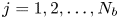 $j=1,2,\ldots,N_b$, with
  $\Delta \varPhi = 2L/(N_f-1)$ and
  $\Delta \phi = 2L/(N_b-1)$. We define the discretised variables at the mesh points,
 \begin{equation} \varTheta_{i}=\theta_f(\varPhi_{i}), \quad Y_i=y_f(\varPhi_i), \quad \theta_{j}=\theta_b(\phi_{j}) , \quad y_j=y_b(\phi_j) , \end{equation}
for  $i=1,2,\ldots,N_f$ and
  $j=1,2,\ldots,N_b$, and the midpoint values
 \begin{equation} \left. \begin{aligned} \varPhi^M_i & = \frac{\varPhi_{i+1} + \varPhi_i}{2}, \quad \phi^M_j = \frac{\phi_{j+1} + \phi_j}{2} , \quad Y^M_i= \frac{Y_{i+1} + Y_i}{2},\\ \varTheta^M_i & = \frac{\varTheta_{i+1} + \varTheta_i}{2}, \quad \theta^M_j = \frac{\theta_{j+1} + \theta_j}{2} , \end{aligned} \right\} \end{equation}
for  $i=1,2,\ldots,N_f-1$ and
  $j=1,2,\ldots,N_b-1$. The discrete form of (3.4), evaluated on
  $\varPhi _i$, is used to define
 \begin{equation} T_{i} \equiv \tau_f(\varPhi_i) = \frac{1}{2}\ln\left( 1 - \frac{2}{F^2}\left(Y_i -1\right)\right)\!, \end{equation}
for  $i=1,2,\ldots,N_f$, which is calculated from the known surface values
  $Y_i$. Using a central difference for the derivative, the values
  $Y_i$ and
  $T_i$ are then inserted into (3.5), yielding
 \begin{equation} \varTheta_i=\arcsin \left(\mathrm{e}^{T_i} \left(\frac{Y_{i+1} - Y_{i-1}}{2\,\Delta\varPhi} \right ) \right)\!, \end{equation}
for  $i=2,3,\ldots,N_f -1$, and we set
  $\varTheta _1 = \varTheta _{N_f}=0$. Now evaluating at the midpoints, and approximating the integrals by the trapezium rule, the discretised form of the integral equation (3.7) is given by
 \begin{align} &\sum_{k=2}^{N_b}\left( \frac{\Delta\phi}{2}\,(G_{b[k-1,i]}\theta_{k-1}+G_{b[k,i]}\theta_k)\right)\nonumber\\ &\quad = \sum_{k=2}^{N_f} \left(\frac{\Delta\varPhi}{2}\,(G_{f[k-1,i]}\varTheta_{k-1}+G_{f[k,i]}\varTheta_k)\right)\nonumber\\ &\qquad -\frac{1}{2}\ln\left( 1 - \frac{2}{F^2}\left(Y^{M}_{i} -1\right)\right)\!, \end{align}
for  $i=1,2,\ldots,N_f-1$, where
 \begin{equation} G_{f[k,i]} = (
1-\mathrm{e}^{{\rm \pi}(\varPhi^{M}_{i} -\varPhi_k
)})^{{-}1} , \quad G_{b[k,i]} =
( 1+\mathrm{e}^{{\rm \pi}(\varPhi^{M}_{i} -
\phi_k)})^{{-}1}.
\end{equation}
\begin{equation} G_{f[k,i]} = (
1-\mathrm{e}^{{\rm \pi}(\varPhi^{M}_{i} -\varPhi_k
)})^{{-}1} , \quad G_{b[k,i]} =
( 1+\mathrm{e}^{{\rm \pi}(\varPhi^{M}_{i} -
\phi_k)})^{{-}1}.
\end{equation}
Now the inverse problem for the unknowns  $\theta _j$ may be written more succinctly as the linear matrix equation
 \begin{equation} \boldsymbol{M} \boldsymbol{\theta}= \boldsymbol{b} , \end{equation}
where  $\boldsymbol {\theta }=(\theta _1,\theta _2\ldots,\theta _{N_b})^\textrm {T}$ is the vector of unknowns,
  $\boldsymbol {b}=(b_1,b_2\ldots,b_{N_f})^\textrm {T}$ is a vector of the known free-surface values
 \begin{equation} b_i =\sum_{k=2}^{N_f} \left(\frac{\Delta\varPhi}{2}\,(G_{f[k-1,i]}\varTheta_{k-1}+G_{f[k,i]}\varTheta_k)\right) -\frac{1}{2}\ln\left( 1 - \frac{2}{F^2}\left(Y^{M}_{i} -1\right)\right)\!, \end{equation}
for  $i=1,2,\ldots,N_f-1$, and
  $\boldsymbol {M}$ is an
  $N_f \times N_b$ matrix with the known elements
  $m_{i,j}$ given by
 \begin{equation} m_{i,1}=\frac{\Delta\phi}{2}\,G_{b[1,i]} , \quad m_{i,N_b}=\frac{\Delta\phi}{2}\,G_{b[N_b,i]} , \quad m_{i,j}=\Delta\phi \, G_{b[j,i]} , \end{equation}
for  $i=1,2,\ldots,N_f-1$ and
  $j=2,3,\ldots,N_b-1$. The final row of the matrix equation is set to enforce a boundary condition. An obvious choice might be to set
  $\theta _{N_b}=0$; however, this condition is already accounted for by the reliance of the conformal mapping on uniform flow far downstream. As such, while it is not in practice necessary to do so, we instead set
  $m_{N_f,1}=1$ and
  $b_{N_f}=0$ to enforce the condition that
  $\theta _1=0$. We found that this greatly improves the conditioning of the system (see figure 3a). To calculate the topography, one would take the solution
  $\boldsymbol {\theta }$ to (3.17) and use these values to evaluate (2.4) at its midpoints, yielding
 $$\begin{gather} \tau^{M}_{j} \equiv \tau_b (\phi^{M}_{j}) = \sum_{k=2}^{N_f} \left(\frac{\Delta\varPhi}{2}\,(g_{f[k-1,j]}\varTheta_{k-1}+g_{f[k,j]}\varTheta_k)\right)\nonumber\\ - \sum_{k=2}^{N_b}\left( \frac{\Delta\phi}{2}\,(g_{b[k-1,j]}\theta_{k-1}+g_{b[k,j]}\theta_k)\right)\! , \end{gather}$$
for  $j=1,2,\ldots,N_{b}-1$, with
 \begin{equation} g_{f[k,j]} = (
1+\mathrm{e}^{{\rm \pi}(\phi^{M}_{j} -\varPhi_k )})^{{-}1}
,\quad g_{b[k,j]} = (
1-\mathrm{e}^{{\rm \pi}(\phi^{M}_{j} - \phi_k)})^{{-}1} .
\end{equation}
\begin{equation} g_{f[k,j]} = (
1+\mathrm{e}^{{\rm \pi}(\phi^{M}_{j} -\varPhi_k )})^{{-}1}
,\quad g_{b[k,j]} = (
1-\mathrm{e}^{{\rm \pi}(\phi^{M}_{j} - \phi_k)})^{{-}1} .
\end{equation}
Finally, by evaluating (2.9) at its midpoints and using a central difference for the derivative, the equation
 \begin{equation} y_{j} = y_{j+1} - \Delta\phi\, \mathrm{e}^{-\tau^{M}_{j}} \sin(\theta^{M}_{j}) \end{equation}
can be used to recover the profile of the topography  $y_b$, working backwards from
  $y_{N_b}=0$, which is set to be consistent with the assumption of a uniform stream downstream.

Figure 3. (a) Dependence of the condition number of  $\boldsymbol {M}$ on
  $N$ when
  $L=10$: (i)
  $\boldsymbol {M}$ with the final row set by the boundary condition
  $\theta _{N}=0$; (ii):
  $\boldsymbol {M}$ with the final row set instead by the boundary condition
  $\theta _1=0$. (b) The eigenfunction of
  $\boldsymbol {M}$ corresponding to the eigenvalue with magnitude
  $9.2\times 10^{-7}$, when
  $L=10$ and
  $N=101$.
Since the matrix  $\boldsymbol {M}$ is expected to be non-singular (we show this to be the case for square
  $\boldsymbol {M}$ in Appendix A), we might follow a direct approach and simply pre-multiply both sides of (3.17) by the matrix inverse to obtain the solution
  $\boldsymbol {\theta }=\boldsymbol {M}^{-1}\boldsymbol {b}$. However, the matrix
  $\boldsymbol {M}$ is very poorly conditioned. This is illustrated in figure 3(a), where we set
  $N_f=N_b=N$ and plot the condition number
  $\textrm {cond}({\boldsymbol {M}})$ against
  $N$ for the truncation length
  $L=10$. The ill-conditioning is considerably worse for the choice of boundary condition
  $\theta _N=0$: even for
  $N=15$, its condition number is of the order of
  $10^{15}$! The ill-conditioning means that in computational practice, for large enough
  $N$, the matrices are effectively singular, and in the case of non-square systems, they are effectively rank deficient. Accordingly, standard approaches to solving (3.17) will be swamped with numerical error as the grid resolution is increased. In particular, the norm of the inverse
  $\| \boldsymbol {M}^{-1}\|$ will be large, and the solution will tend to align itself with the eigenfunction corresponding to the smallest magnitude eigenvalue. Figure 3(b) shows the eigenfunction of
  $\boldsymbol {M}$ associated with the eigenvalue
  $9.2\times 10^{-7}$, when
  $N=101$ and
  $L=10$. The eigenfunction has a non-smooth sawtooth appearance.
To mitigate the difficulties with the ill-conditioning, we employ the TSVD method (e.g. Varah Reference Varah1973; Hansen Reference Hansen1990), to be discussed below. In the standard implementation of the singular value decomposition method (e.g. Griffel Reference Griffel1989), the  $N_f\times N_b$ matrix
  $\boldsymbol {M}$ is expressed in the form
  $\boldsymbol {M}=\boldsymbol {U}\boldsymbol {\varSigma }\boldsymbol {V}^\textrm {T}$, where
  $\boldsymbol {U}$ and
  $\boldsymbol {V}$ are, respectively,
  $N_f\times N_f$ and
  $N_b\times N_b$ unitary matrices whose columns are the eigenvectors of
  $\boldsymbol {M}\boldsymbol {M}^\textrm {T}$ and
  $\boldsymbol {M}^\textrm {T}\boldsymbol {M}$, respectively. The
  $N_f\times N_b$ matrix
  $\boldsymbol {\varSigma }$ has along its leading diagonal the singular values
  $\sigma _n$,
  $n=1,\ldots,r\leq \min (N_f,N_b)$, corresponding to the positive square roots of the non-zero eigenvalues of
  $\boldsymbol {M}\boldsymbol {M}^\textrm {T}$, and all other elements zero. The singular values are ordered by size starting with the largest in the
  $(1,1)$ position.
Armed with the singular value decomposition, we compute the Moore–Penrose inverse (Penrose Reference Penrose1955)  $\boldsymbol {M}^+=\boldsymbol {V}\boldsymbol {\varSigma }^+\boldsymbol {U}^\textrm {T}$, where
  $\boldsymbol {\varSigma ^+}$ is formed by replacing the non-zero entries of
  $\boldsymbol {\varSigma }$ with their reciprocals and then transposing the matrix (e.g. Ben-Israel & Greville Reference Ben-Israel and Greville2003, p. 207). (Note that if
  $\boldsymbol {M}^{-1}$ exists, then
  $\boldsymbol {M}^+=\boldsymbol {M}^{-1}$.) A solution to (3.17) exists if and only if the solvability condition
  $\boldsymbol {M}(\boldsymbol {M}^+\boldsymbol {b})=\boldsymbol {b}$ holds; this ensures that
  $\boldsymbol {b}\in \mbox {Im}\,\boldsymbol {M}$. Then the complete set of solutions to (3.17) is given by (e.g. James Reference James1978)
 \begin{equation} \boldsymbol{\theta}= \boldsymbol{M}^+\boldsymbol{b} + \boldsymbol{z}, \end{equation}
where  $\boldsymbol {z} = (\boldsymbol {I}-\boldsymbol {M}^+\boldsymbol {M})\boldsymbol {w}$, with
  $\boldsymbol {w}$ an arbitrary
  $N_b \times 1$ vector, and
  $\boldsymbol {z} \in \mbox {ker}\,\boldsymbol {M}$. If the solvability condition fails, then
  $\boldsymbol {b}\notin \mbox {Im}\,\boldsymbol {M}$, the system (3.17) is inconsistent, and (3.23) provides the linear least squares approximation of minimum norm (e.g. Planitz Reference Planitz1979).
We will discuss results for the inverse topography problem allowing for different numbers of grid points on the free surface and on the bottom, taking  $N_f>N_b$ (overdetermined system), or
  $N_f< N_b$ (underdetermined system), or else
  $N_f=N_b$ (square system). Since if
  $N_f\geq N_b$ we expect
  $\boldsymbol {M}$ to have full rank, its kernel should be trivial so that the unique solution to (3.17) is given by (3.23) with
  $\boldsymbol {z}$ set to zero. However, in computational practice
  $\boldsymbol {M}$ is effectively rank deficient, as discussed above, so that the kernel is effectively non-trivial. Accordingly, we expect that artificial sawtooth irregularities, like those seen in the eigenfunction in figure 3(b), will become a dominant feature of the numerical solution as the grid resolution is refined. To work around this, we follow the TSVD method (e.g. Varah Reference Varah1973; Hansen Reference Hansen1990) and replace
  $\boldsymbol {M}$ in (3.17) with
  $\boldsymbol {M}_k = \boldsymbol {U}\boldsymbol {\varSigma }_k^+ \boldsymbol {V}^\textrm {T}$, where
  $\boldsymbol {\varSigma }_k^+$ is the rank
  $k$ matrix obtained by retaining the first
  $k$ largest singular values and setting the others to zero. The resulting rank
  $k$ approximate problem has least squares solutions of the form given in (3.23) with
  $\boldsymbol {M}^+$ replaced by
  $\boldsymbol {M}^+_k$. We find that the smoothest solution is that which minimises
  $\|\boldsymbol {\theta }_k\|$:
 \begin{equation} \boldsymbol{\theta_k} = \boldsymbol{M}_k^+ \boldsymbol{b} . \end{equation}
 To illustrate the procedure, we return to the test topography (2.12) examined in figure 2. The free-surface profile is computed first by solving the forwards problem using Newton's method. Next, the inverse problem is solved with the forwards solution as input using the TSVD approach just described. Figure 4(a) shows the logarithm of the norm  $\|\boldsymbol {\theta _k}\|$ for the inverse problem plotted against
  $k$ on a logarithmic scale. We see that
  $\|\boldsymbol {\theta _k}\|$ reaches a plateau that extends over a wide range of
  $k$ values; thereafter, the norm increases as
  $k$ approaches
  $N$, and the numerical problems discussed above become prominent. The profile of
  $\boldsymbol {\theta _k}$ plotted against
  $\phi$ is found to be visually smooth, and to remain the same, over the plateau region. Typical profiles for various
  $k$ are shown in figure 4(b). The characteristic sawtooth numerical instability is evident for
  $k=330$. Typically, when solving the inverse problem, we produce a graph similar to that shown in figure 4(a) to confirm the presence of a plateau. We then choose a value of
  $k$ towards the rightmost end of the plateau in order to retain as many of the original singular values of the original matrix
  $\boldsymbol {M}^+$ as possible. Finally, we compute the topographic profile
  $y_b(\phi )$ using (3.22).

Figure 4. Results for the topography (2.12) at  $F=1.2$ when
  $L=20$ and
  $N=363$. (a) Values of
  $\|\boldsymbol {\theta _k}\|$ rise rapidly to a stable value for a range of the truncation parameter
  $k$ before beginning to increase further as the model fails to output smooth solutions. (b) Profiles of
  $\boldsymbol {\theta _k}$ for various
  $k$, showing how the output varies by selecting
  $k$ to correspond to the different sections of the
  $(k,\|\boldsymbol {\theta _k}\|)$ curve.
Figure 5 shows a convergence study for the test topography (2.12) for a square system with  $N_f=N_b=N$. In figure 5(a), we see good agreement between the exact topography (2.12), shown with a thick solid line, and the output from the inverse problem, shown for the two different discretisation levels
  $N=101$ and
  $N=721$ with a thin solid and a dotted line, respectively. In figure 5(b), we plot the norm of the difference
  $\| y_b - y_T \|$ over the grid, where
  $y_T$ is the prescribed topography given by (2.12), and
  $y_b$ is the inversely computed topography. The error
  $\| y_b - y_T \|$ decreases like
  $N^{-2}$ as
  $N$ increases. Unless otherwise stated, in each of the results presented in the next section, the inversely found bottom profiles were used as input to the forwards problem to check that the original free surface is recovered. While it is straightforward to do this for either subcritical or supercritical Froude number, the critical case
  $F=1$ is computationally more challenging (Keeler, Binder & Blyth Reference Keeler, Binder and Blyth2017).

Figure 5. The case of topography (2.12) at  $F=1.2$ when
  $L=20$ and
  $N=101$. (a) The originally prescribed topography compared to those found by applying the TSVD method to the results of the forwards Newton problem at two resolutions (
 $k=101$,
  $N=101\ {\rm or}\ 721$). (b) The norm of the error
  $\| y_b-y_T\|$, where
  $y_T$ is the prescribed topography (2.12), and
  $y_b$ is the TSVD solution.
4. Results
In this section we discuss solutions to the inverse pressure and topography problems when the free surface is prescribed with the Gaussian form
 \begin{equation} y_f=1+\alpha\,\mathrm{e}^{-(\beta \phi)^2}, \end{equation}
where  $\alpha$ and
  $\beta$ are parameters that control the amplitude and width of the free-surface disturbance, respectively. In each case, we solve the inverse problem using the TSVD method described in the preceding section for various values of the Froude number
  $F$. We note that if
  $\alpha =0$, so that the free surface is flat, then
  $\boldsymbol {b}=\boldsymbol {0}$ in (3.17). Since
  $\boldsymbol {M}$ is non-singular, it follows that
  $\boldsymbol {\theta }=\boldsymbol {0}$ and the topography is also flat. This agrees with the result derived above that the only solution to the homogeneous form of the integral equation (3.7) (with
  $b\equiv 0$) is
  $\theta =0$, so that a flat free surface corresponds to a flat bottom.
In figure 6(a), we show computed topography profiles for a range of subcritical to supercritical Froude numbers. It can be seen that the topography changes from a dip to a rise over this range of  $F$, with the central response
  $y_b(0)$ changing sign as
  $F$ increases. It is interesting to note that the supercritical solutions shown in figure 6(a) can be categorised as a perturbation of a solitary wave. Solutions that are perturbations to the uniform stream in supercritical flow will feature a free surface that follows the shape of the topography; here, the supercritical solutions are found to have a depression in the topography, underlying an elevation on the surface. Further, the maximum elevation of the free surface, for the two solutions with
  $F > 1$, is close to the maximum elevation of the free solitary wave,
  $\eta (0) \approx 2(F - 1)$. The corresponding perturbation of a uniform stream solution can be obtained by taking the inversely found topography with an initial guess of a flat free surface as input in the forwards problem, yielding forward free-surface solutions that simply follow the shape of the topographies. We note that this does not mean that all supercritical inverse solutions will be categorised as a perturbation of a solitary wave; the classification needs to be determined on a case by case basis.


Solutions to the inverse pressure problem are obtained by making the approximation (Binder et al. Reference Binder, Blyth and McCue2013)
 \begin{equation} \theta_f \approx \arctan \left(\frac{\partial y_f}{\partial \phi}\right) \end{equation}
and then using (3.3) to calculate the pressure. Figure 6(b) shows the pressure forcing found in this way for the same free surface and over the same range of Froude numbers as in figure 6(a).
Figure 7(a) compares the norms of the computed inverse topography,  $\|y_b\|$, the approximated pressure forcing,
  $\|P\|$, and the forcing predicted by the fKdV equation (3.2),
  $\|\,f\|$, for the free surface (4.1), with
  $\phi$ replaced by
  $x$, over a range of
  $F$. The fKdV norm is given by
 \begin{equation} \|\,f\| = \left|\alpha{\rm \pi}^{1/4}\right| \sqrt{ \frac{4(F-1)^2}{\beta\sqrt{2}} + \frac{4\beta(F-1)+\beta^3}{3\sqrt{2}} - \frac{6\alpha(F-1)}{\beta\sqrt{3}}- \frac{4\alpha\beta}{3\sqrt{3}} +\frac{9\alpha^2}{8\beta}} , \end{equation}
and its minimum occurs at  $F = 1+ \alpha \sqrt {6}/4 - \beta ^2/6$.

Figure 7. Inverse problems for the free surface (4.1) with  $\alpha =0.2$ and
  $\beta =0.3$, and
  $L=20$ and
  $N=641$. (a) The norms of the forcing found by the inverse pressure method (dotted line), the TSVD inverse topography method (dashed line) and the fKdV model (solid line) as the Froude number
  $F$ is varied. (b) The corresponding values of the forcing at
  $x=\phi =0$ for the results shown in (a).
Despite the appearance on the scale shown, there is no single point of intersection between the three norm curves. However, the intersections occur at approximately  $F=1$. In subcritical flow, the topography has the greatest norm and is also the most sensitive to varying
  $F$: the greatest change in the norm for any change in
  $F$ occurs for the topographic norm. In the supercritical regime, the topographic norm reaches a minimum at
  $F=1.07$, which is lower than the value
  $F=1.11$ predicted by the fKdV equation (3.2), although the minimum norm value is estimated reasonably well by the fKdV equation. There is good agreement between the pressure norm and the fKdV norm, but the topographic norm is larger than the fKdV norm over much of the range shown. Both the pressure norm and the topography norm have a local minimum in the plotted domain, as was predicted by the fKdV model; however, the exact value for
  $F$ and the corresponding norm at which the minimum occurs varies depending on the type of forcing.
According to the fKdV equation, the size of the forcing at the point of symmetry,  $x=0$, varies linearly with
  $F$ such that
  $f(0)=\alpha (2(F-1)+2\beta ^2/3-3\alpha /2)$. This behaviour is compared with that seen for the inverse pressure and topography problems in figure 7(b). Once again, we see good agreement between the fKdV prediction and the inverse pressure response, while the topographic response shows a much stronger deviation away from
  $F=1$. The intersections of the three curves are clustered near
  $F=1.02$, and all models give similar predictions near this value. Away from this point, changes in
  $F$ elicit much larger topographic responses.
Thus far, we have presented results for systems for which the matrix  $\boldsymbol {M}$ in (3.17) is square with
  $N_f=N_b=N$. However, the ability to reduce the number of measurements on the surface or desired resolution on the topography and still obtain accurate results has immediate practicality. Measurements may be difficult to take and so be limited in number, or we might be interested only in the broad qualitative features of the topography and so be able to reduce computational complexity by taking fewer points.
Figure 8 shows the topography norm plotted against  $F$ for the Gaussian free surface (4.1) and various levels of model resolution, corresponding to an overdetermined system (
 $N_f>N_b$), an underdetermined system (
 $N_f< N_b$), a square system with a low value of
  $N$, and a square system with a higher value of
  $N$. At the plotted resolutions, it can be seen that all four norm curves follow one another closely. Above a threshold resolution for the input data (
 $N_f\approx 80$ for figure 8), the norm is insensitive to the choice of
  $N_f$ or
  $N_b$. However, for values
  $N_f<80$, the four curves in figure 8 are separated into two pairs (each pair for one value of
  $N_f$ and two values of
  $N_b$), with the separation distance between them increasing as
  $N_f$ decreases. Once
  $N_f$ is sufficiently large, both pairs are close together, as in figure 8, and the choice of the value of
  $N_b$ is less important.

Figure 8. Inverse topography problem for the free surface (4.1) with  $\alpha =0.2$ and
  $\beta =0.3$, for
  $L=20$ and various grid resolutions: lower-resolution square system (solid line), underdetermined system (dash-dotted line), overdetermined system (dotted line) and higher-resolution square system (dashed line), for combinations of taking
  $81$ and
  $641$ mesh points. The value of
  $k$ was taken to be the largest possible value from the set
  $\{41,81,158\}$ subject to
  $k\leq \min (N_f,N_b)$.
Figure 9 shows inverse solutions for non-Gaussian surface data, instead taking on the surface a finite train of waves. In figure 9(a), input data  $y_f$ were generated by first solving the forwards problem for a subcritical flow over two identical Gaussian topographical features, i.e.
 \begin{equation} y_T=a (\mathrm{e}^{-(b(\phi+c))^2} +\mathrm{e}^{-(b(\phi-c))^2}), \end{equation}
while allowing the separation  $c$ to come as part of the solution; this approach yields a solution featuring a train of trapped surface waves between the two topographical features. The inverse solution for
  $F=0.8$ recovers the originally prescribed
  $y_T$. As
  $F$ is varied, the form of the solution changes from having two distinct Gaussian disturbances to instead feature a train of repeating undulations in the topography over approximately the same support as the surface data. Figure 9(b) shows the inverse solutions for surface data prescribed directly in the form
 \begin{equation} y_f=1+\frac{\alpha}{2}\left(\tanh\left(\beta(\phi+C)\right)-\tanh(\beta(\phi-C))\right)\cos(\phi) . \end{equation}
Figure 9. Inverse problem solutions for two fixed free surfaces at different Froude numbers. (a) Free surface (blue) obtained as a solution to the forwards problem, with  $F=0.8$, over a topography given by (4.4), with
  $a=-0.04$,
  $b=1$,
  $c\approx 10.14$,
  $L=30$,
  $N=1624$. (b) Free surface (blue) prescribed directly as (4.5) with
  $\alpha =0.1$,
  $\beta =1.2$,
  $C\approx 20.42$,
  $L\approx 40.84$,
  $N=1624$.
5. Application to noisy input data
In practice the inverse topography problem would receive as input noisy measurements of  $y_F$. Given that the problem formulation via the integral equation (3.7) is ill-posed, this section performs a careful assessment of the performance of our numerical approach in the presence of fluctuations in the input data. In § 5.1, we implement a fast and rigorous uncertainty quantification method to estimate the bottom topography.
As in § 3.3.1, we let  $Y_i$ denote the surface height at the
  $i$th grid point, but suppose that the
  $Y_i$ are unknown. In their place, we suppose that we observe measurements
  $\tilde {Y}_i$ that are corrupted by small surface disturbances and measurement errors,
 \begin{equation} \tilde{Y}_i\mid Y_i \sim \mathcal{N}(Y_i,\sigma^2) \text{ independently for } i=2,\ldots, N_f-1, \end{equation}
for some known variance  $\sigma ^2$. The notation ‘
 $a \mid b$’ means ‘the probability distribution function of
  $a$, given perfect knowledge of
  $b$’, and the use here codifies how the noisy observations would be drawn if we knew the surface heights
  $Y_i$ exactly. An example using the Gaussian form (4.1) is shown in figure 10(a). In order to not violate our requirements of uniform flow both upstream and downstream, we do not add noise to the first and final mesh points, i.e.
  $\tilde {Y}_1 = Y_1$ and
  $\tilde {Y}_{N_f} = Y_{N_f}$. Equivalently, we may append to the measurement data two more data points corresponding to the uniform stream.

Figure 10. (a) Example of noise-contaminated surface (grey); noise drawn from a normal distribution with standard deviation  $\sigma =5\times 10^{-3}$ has been added to the free surface (black), with
  $\alpha =0.2$,
  $\beta =0.3$,
  $F=1.2$,
  $L=25$,
  $N=341$,
  $k=40$. (b) By calculating TSVD solutions (two randomly chosen noisy solutions are highlighted (black dotted) on top of all output solutions (grey)) to 1000 random-noise-contaminated surfaces, an estimate for the true topography (black solid line) can be obtained by averaging the noisy solutions.
Application of the TSVD method described above to these noisy input data yields an output for the shape of the topography, typical outputs for which can be seen as the grey curves in figure 10(b). We found that repeating this process and then calculating the mean of the resultant set of noisy solutions, at each value of  $\phi _j$, allows for an approximation of the solution to the underlying unperturbed problem, shown as the black solid curve in figure 10(b). However, the perturbed problem is much more sensitive to the choice of the truncation rank
  $k$ than the unperturbed problem. We found that the profiles of the
  $(k,\|\boldsymbol {\theta _k}\|)$ curves no longer have a single uninterrupted flat region, like that of the unperturbed problem shown previously in figure 4(a). Instead, they have a stepped shape with no clear interval from which to select a value for
  $k$. We opt to use the unperturbed problem as a guide, selecting a value of
  $k$ for which the unperturbed
  $(k,\|\boldsymbol {\theta _k}\|)$ curve has flattened, so the output for that problem should well approximate
  $\theta _b$. In the unperturbed problem,
  $k$ was chosen to be as large as possible while remaining on the flat region of the
  $(k,\|\boldsymbol {\theta _k}\|)$ curve. However, for the perturbed problem, we instead take
  $k=40$ to be on the lower end of this region in order to avoid the magnification of errors in the input data that will occur for the higher values of
  $k$.
$k$.
Figure 10 demonstrates for our example problem that the TSVD method generates bottom topographies that are noisy perturbations of the true bottom topography, and that given sufficient data, the mean of these perturbations is close to the true mean. The next subsection introduces an uncertainty quantification procedure to compute a confidence interval around estimates of the bottom topography. We highlight that this procedure can be used even in the case of a single observation of the surface.
5.1. Uncertainty quantification
In this subsection, we continue to interpret  $\tilde Y_i$, the data measurements at the surface, as random perturbations of the unknown true surface values
  $Y_i$. In principle, one may obtain the exact probability distribution of the bottom topography
  $y_j$ as follows. The quantities in (3.13)–(3.22), which involve either a linear or nonlinear dependence on
  $Y_i$, are now random variables. Their distributions may in principle be calculated by transforming the distribution of
  $Y_i$ and multiplying by a suitable Jacobian (e.g. Casella & Berger Reference Casella and Berger2021), yielding the exact probability distribution function for the bottom topography. However, the computation is intensive, and the result will probably not follow any known distribution, hence would be difficult to interpret.
Whilst obtaining the analytical result may be of possible future interest, we instead employ here a rapid and effective sampling strategy that leverages the computational speed of the TSVD inverse method. The idea is to repeatedly perturb the observed data points  $\tilde Y_i$ and, independently for each perturbed pseudo-observation, use (3.13)–(3.22) to obtain a topography estimate for the pseudo-observation. The many pseudo-observations capture the uncertainty in the measurements
  $\tilde Y_i$, and the topography estimates capture accurately the uncertainty in the topography estimates.
To be precise, we note that the unknown idealised surface measurements  $Y_i$ are near to the noisy observations
  $\tilde Y_i$, and in fact,
  $Y_i\mid \tilde Y_i \sim \mathcal {N}(\tilde Y_i,\sigma ^2).$ Fixing some integer
  $n$ number of pseudo-observations, we define
 \begin{equation} Y_{ik} := \tilde Y_i + \eta_{ik} \end{equation}
independently for  $i=2,\ldots,N_f-1$ and for
  $k = 1,\ldots, n$, where
  $\eta _{ik} \sim \mathcal {N}(0,\sigma ^2)$, and
  $\sigma$ is supposed to be known or estimated from data.
The next step is to plug the  $Y_{ik}$ into the inverse method derived in § 3.3.1. Prior to doing this, we note that the standard deviation
  $\sigma$, which is presumed known, represents the measurement error. In practice, usually it must be estimated. The number of pseudo-observations to use,
  $n$, must be chosen. As we will see, as
  $n\rightarrow \infty$, the proposed method converges to the exact distribution. In practice, moderate choices
  $n\approx 30$ are often sufficient; a simple measure of agreement is to test two values of
  $n$ and confirm whether the mean and standard deviation of the resulting topography estimates agree sufficiently for the problem at hand.
The  $Y_{ik}$ are Monte Carlo samples of possible values of
  $Y_i$ from the distribution
  $Y_i \mid \tilde Y_i$. Formally,
 \begin{equation} p( Y_i\mid \tilde Y_i ) \approx \frac 1n \sum_{k=1}^{n} \delta(Y_i - Y_{ik}), \end{equation}
where  $p(\ \cdot\ )$ means the probability distribution function, and
  $\delta (\ \cdot\ )$ is the Dirac delta function. While the weighted sum in (5.3) is difficult to interpret, its cumulative density function is simply a step function that increments by
  $1/n$ at each
  $Y_{ik}$. The sampled cumulative density function converges as
  $n\rightarrow \infty$, as do all moments of the approximation (5.3), in the usual Monte Carlo fashion (Kroese, Taimre & Botev Reference Kroese, Taimre and Botev2013).
The bottom topography  $y_j$ at grid point
  $j$ can be written as a nonlinear function of the surface observations,
  $y_j = g(Y_1,\ldots,Y_{N_f};j)$, where
  $g(\ \cdot\ )$ is a shorthand that means applying (3.13)–(3.22), and formally, it also depends on the parameters listed therein. For conciseness, we write the unknown free surface
  ${\boldsymbol Y} = (Y_1,\ldots, Y_{N_f})$, the observations
  $\tilde {\boldsymbol Y} = (\tilde Y_1,\ldots,\tilde Y_{N_f})$ and the pseudo-observations
  ${\boldsymbol Y}_k = (Y_{1k},\ldots, Y_{N_f k})$. Then, using (5.3),
 \begin{equation} p(\kern0.7pt y_j \mid \tilde {\boldsymbol Y} ) = \int_{\mathbb{R}^{N_f}} p(\kern0.7pt y_j\mid {\boldsymbol Y} )\, p({\boldsymbol Y} \mid \tilde {\boldsymbol Y} ) \,{\rm d}{\boldsymbol Y} \approx \frac 1n \sum_{k=1}^{n} \delta(\kern0.7pt y_j - g({\boldsymbol Y}_{k};j) ), \end{equation}
where  $p(\kern0.7pt y_j \mid \tilde {\boldsymbol Y} )$ means the probability distribution function for the bottom topography given the observed data. This general result clarifies that the pseudo-observations
  ${\boldsymbol Y}_k$, transformed into estimates of the bottom topography by the action of
  $g({\boldsymbol Y}_{k};j)$, fully capture the uncertainty in the estimate of that topography.
In the interesting case of large  $N$, here corresponding to densely packed data on the surface, we make one modification to (5.4) to accommodate a weakness of the approach: the distribution (5.4) does not encode our belief that the unknown true surface
  $Y$ is smooth. As the TSVD method in § 3.3.1 involves solving a discretised equation numerically, components of the solution depend on
  $1/(\Delta \varPhi ) \propto N$, so increasing
  $N$ worsens the accuracy of the solution due to compounding numerical error. We can mitigate this numerical instability at large
  $N$ by smoothing the solution, without compromising statistical rigour, as follows. We choose an integer
  $\varGamma >0$ and a smoothing method; here, we interpolate data points onto a quadratic of best fit. We then divide the locations
  $\varPhi _i$ at which surface measurements are available into non-overlapping intervals, each containing
  $2\varGamma +1$ points. In each of these intervals, we compute the smoothing method and evaluate it at the central grid point of that interval. The total number of grid points
  $N$ reduces to
  $\hat N \approx N/(2\varGamma +1)$.
Our proposed algorithm is as follows. For each grid point  $j$, we compute
 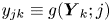 $y_{jk} \equiv g({\boldsymbol Y}_{k};j)$ and then record the mean and variance of these ‘bottom topography samples’. Figure 11 shows clearly that the algorithm produces appropriate mean estimates and confidence intervals. Figures 11(a,b) show results for a single noisy observation of the free surface and for ten such observations, respectively (compare figure 10(b), which employs one thousand observations). In both plots of figure 11, it can be seen that plotting the mean topography estimate plus or minus three times the standard deviation of the estimates provides a bounded region within which the true topography lies. Furthermore, figure 11(b) demonstrates that repeated independent observations of the surface provide sufficient information to estimate the bottom topography accurately.

Figure 11. Plots for  $\alpha =0.2$,
  $\beta =0.3$,
  $F=1.2$,
  $L=25$,
  $N=361$,
  $k=40$,
  $\sigma =5\times 10^{-3}$,
  $n=50$: (a) inference from a single observation of the surface heights; (b) inference from ten observations of the surface heights. We show the unperturbed topography solution (brown solid line), topography estimates given by the mean of
  $y_{jk}$ (blue circles), and a three-standard-deviation confidence interval (blue dots).
6. Conclusions
We have considered how the inverse problem for topography is an ill-posed inverse problem and how issues with numerical instability of the solutions with increasing resolution are inherent to the problem. We presented a method for calculating quickly approximate regularised solutions for the topography that are in agreement with solutions found previously at a low resolution using the Newton method, results themselves found to agree well with the experimental observations of Tam et al. (Reference Tam, Yu, Kelso and Binder2015). By averaging the outputs from perturbed noisy surfaces, we were able to obtain the underlying topography to a good accuracy, and saw that by ensuring the endpoints are kept noise-free, the outputs are generally much more accurate to the true solution, with less deviation between them. As the downstream flow should be uniform by construction of the model, one can simply extend the data by appending to them a region with a flat free surface.
Future work includes the testing of the model on different surface profiles, such as wave-trains or hydraulic falls, and how the presence of noise in these surfaces affects the quality of the solution. Derivation of the model allows for combined forcing situations; however, in the event that both pressure and topography are unknown simultaneously, one would expect an infinite number of solutions, so thought is needed here on how the problem might be constrained further. More research is needed into systematically choosing a truncation rank for the problem, especially as the free surface is allowed to become more complicated and a higher resolution is needed in order to sufficiently capture its details. Preliminary work on error-contaminated problems has been promising, but further study is needed, alongside an investigation of whether any results might be extended into three-dimensional models.
Declaration of interests
The authors report no conflict of interest.
Appendix A. The determinant of  ${M}$
${M}$

We examined carefully the exact form of the determinant of the square  $N\times N$ matrix
  $\boldsymbol {M}$ in (3.17). By experimenting using the computer algebra package Maple, we found that the determinant may be expressed as
 \begin{equation} \mbox{det}\,\boldsymbol{M} = \frac{1}{2} \prod_{k=1}^{2N-3} ({-}1)^{N-1}x^{\kern 0.06em N-1}(x^k+1)^{a(k)}(x^k-1)^{b(k)}, \end{equation}
where  $x = \exp ({\rm \pi} h/2)$, and the exponents
  $a(k)$,
  $b(k)$ are integers. It does not appear to be a simple matter to give the functional forms of
  $a$ and
  $b$, but for our purposes it suffices to know that they are integers. According to (A1),
  $\mbox {det}\,\boldsymbol {M}=0$ only if
  $x=0$ or
  $x=1$. It follows that
  $\det \boldsymbol {M}\neq 0$ if
  $h>0$, and therefore
  $\boldsymbol {M}$ has full rank for any non-zero grid spacing.


 Open access