


1. Introduction
Definition 1. Let H be a constant belonging to (0, 1). A fractional Brownian motion (fBm) $(W^H_{t})_{t \geq 0}$
with Hurst parameter H is a continuous and centred Gaussian process with covariance function
$(W^H_{t})_{t \geq 0}$
with Hurst parameter H is a continuous and centred Gaussian process with covariance function
 \begin{align*}\mathrm{E}\, \left[W^H_{t} W^H_{s}\right] = \frac{1}{2}\big(t^{2H} + s^{2H} - |t-s|^{2H}\big). \end{align*}
There are a few important properties of fBm, including self-similarity, long dependence for $H > \frac{1}{2}$
, and stationary increments.
$H > \frac{1}{2}$
, and stationary increments.
Mandelbrot and Van Ness [Reference Mandelbrot and Van Ness31] introduced fBm in 1968. It is a family of Gaussian random functions with a Hurst parameter H. The paper suggested that the fBm with Hurst parameter H is a moving average of $\mathrm{d}B(t)$
in which past increments of B(t) are weighted by the kernel
$\mathrm{d}B(t)$
in which past increments of B(t) are weighted by the kernel $(t-s)^{H-1/2}$
. Therefore, the increment process of fBm can be viewed as long-time correlated white noise.
$(t-s)^{H-1/2}$
. Therefore, the increment process of fBm can be viewed as long-time correlated white noise.
Gatheral [Reference Gatheral, Jaisson and Rosenbaum20] suggested that log-volatility can be approximated by an fBm with a Hurst parameter of around $0.1$
. This gives rise to new pricing models that make use of fBm to model volatility.
$0.1$
. This gives rise to new pricing models that make use of fBm to model volatility.
In this work we improve the so-called fast algorithm by Jing Tang Ma et al. [Reference Ma and Wu30] and as a result develop a new algorithm for simulating fBm and multivariate fractional Brownian motion (mfBm), and compare it with the known state of the art. Our algorithm is approximately an order of magnitude faster than the nearest competitor. We then apply our results to option pricing.
The code behind this paper can be found in our open source Python library for simulating fBm and mfBm: https://github.com/kaiboy05/fbm.
Our work provides limited background on fBm and mfBm. For rigorous mathematical expositions, the reader can consult [Reference Banna, Mishura, Ralchenko and Shklyar3, Reference Biagini, Hu, Øksendal and Zhang7, Reference Mishura32, Reference Nourdin34]. For a mathematically rigorous treatment of the corresponding option pricing models, including the asymptotic analysis, the reader can consult [Reference Bonesini, Jacquier and Pannier8, Reference Guennoun, Jacquier, Roome and Shi21, Reference Horvath, Jacquier and Muguruza24, Reference Jacquier, Pakkanen and Stone28, Reference Pakkanen and Réveillac35].
2. Testing and comparing the simulation methods
In order to verify that the simulation methods in Section 3 have been implemented correctly, we need a set of statistical criteria to verify that the generated paths have the correct behaviour, that is, the fBm has the covariance structure as in Definition 1. In this section, two such methods of testing will be introduced.
2.1. Likelihood ratio test
The first method is the likelihood ratio test [Reference Casella and Berger10], which is a general way to test if a set of paths have a specified covariance matrix.
Definition 2. If $X_1, \ldots, X_n$
is a random sample from a population with probability density function (PDF) or probability mass function (PMF)
$X_1, \ldots, X_n$
is a random sample from a population with probability density function (PDF) or probability mass function (PMF) $f(x|\theta)$
(
$f(x|\theta)$
( $\theta$
may be a vector), the likelihood function is defined as
$\theta$
may be a vector), the likelihood function is defined as
 \begin{align*}L(\theta|x_1, \ldots, x_n) = L(\theta|\mathbf{x}) = f(\mathbf{x}|\theta) = \prod^n_{i=1}f(x_i|\theta). \end{align*}
Remark 1. Here $f(\mathbf{x}|\theta)$
is the PDF or PMF with parameter
$f(\mathbf{x}|\theta)$
is the PDF or PMF with parameter $\theta$
.
$\theta$
.
Definition 3. Let $\Theta$
denote the entire parameter space. The likelihood ratio test statistic for testing
$\Theta$
denote the entire parameter space. The likelihood ratio test statistic for testing $H_0:\theta\in \Theta_0$
versus
$H_0:\theta\in \Theta_0$
versus $H_1:\theta \in \Theta \backslash \Theta_0$
is
$H_1:\theta \in \Theta \backslash \Theta_0$
is
 \begin{align*}\Lambda(\mathbf{x}) = \frac{\sup_{\Theta_0} L(\theta|\mathbf{x})}{\sup_{\Theta} L(\theta|\mathbf{x})}. \end{align*}
A likelihood ratio test (LRT) is any test that has a rejection region (R) of the form $R = \{\mathbf{x}: \Lambda(\mathbf{x}) \leq c\}$
, where c is any number satisfying
$R = \{\mathbf{x}: \Lambda(\mathbf{x}) \leq c\}$
, where c is any number satisfying $0 \leq c \leq 1$
.
$0 \leq c \leq 1$
.
Definition 4. For $\alpha \in [0, 1]$
, a test is a level
$\alpha \in [0, 1]$
, a test is a level $\alpha$
test if
$\alpha$
test if $\sup_{\theta \in \Theta_0} P_\theta(\mathbf{X} \in R) \leq \alpha$
.
$\sup_{\theta \in \Theta_0} P_\theta(\mathbf{X} \in R) \leq \alpha$
.
The LRT compares the largest likelihood among the whole parameter space with the largest likelihood among the hypothesis parameter region. If the ratio is small, then it means it is more likely that the null hypothesis is wrong, and vice versa. Note that the maximum likelihood estimator (MLE) is the estimator of $\theta \in \Theta$
that gives the largest likelihood value. Hence, the denominator is the likelihood value of the MLE in
$\theta \in \Theta$
that gives the largest likelihood value. Hence, the denominator is the likelihood value of the MLE in $\Theta$
, while the numerator is the likelihood of the MLE in
$\Theta$
, while the numerator is the likelihood of the MLE in $\Theta_0$
. Therefore, if both the likelihood values are closed (i.e.
$\Theta_0$
. Therefore, if both the likelihood values are closed (i.e. $\Lambda(\mathbf{x}) \approx 1$
), then there is a larger chance that the
$\Lambda(\mathbf{x}) \approx 1$
), then there is a larger chance that the $\theta \in \Theta_0$
, thus favouring the hypothesis
$\theta \in \Theta_0$
, thus favouring the hypothesis $H_1$
.
$H_1$
.
Assume we have n samples of multivariate normal variables, $\mathbf{X}_1, \mathbf{X}_2, \ldots, \mathbf{X}_n$
, where
$\mathbf{X}_1, \mathbf{X}_2, \ldots, \mathbf{X}_n$
, where $\mathbf{X}_k$
is a column vector such that
$\mathbf{X}_k$
is a column vector such that $\mathbf{X}_k = (X_{k1}, X_{k2}, \ldots, X_{kp})^{\top}$
for
$\mathbf{X}_k = (X_{k1}, X_{k2}, \ldots, X_{kp})^{\top}$
for $k=1,2,\ldots,n$
. In addition, assume the multivariate normal variables have (column) mean vector
$k=1,2,\ldots,n$
. In addition, assume the multivariate normal variables have (column) mean vector $\boldsymbol{\mu} = (\mu_1, \mu_2, \ldots, \mu_p)^{\top}$
and covariance matrix
$\boldsymbol{\mu} = (\mu_1, \mu_2, \ldots, \mu_p)^{\top}$
and covariance matrix $\boldsymbol{\Sigma}$
, a
$\boldsymbol{\Sigma}$
, a $p \times p$
positive definite matrix. Then the likelihood function is given by
$p \times p$
positive definite matrix. Then the likelihood function is given by
 \begin{align*}L(\mathbf{X}_1, \ldots, \mathbf{X}_n|\boldsymbol{\mu}, \boldsymbol{\Sigma}) = \frac{1}{(2\pi)^{np/2}|\boldsymbol{\Sigma}|^{n/2}}\prod^{n}_{k=1}\exp \Big[-\frac{1}{2}(\mathbf{X}_k - \boldsymbol{\mu})^{\top}\boldsymbol{\Sigma}^{-1}(\mathbf{X}_k - \boldsymbol{\mu})\Big]. \end{align*}
Since we want to test if the samples’ covariance matrix is equal to the expected covariance matrix or not, our hypotheses are $H_0:\boldsymbol{\Sigma} = \boldsymbol{\Sigma}_0$
and
$H_0:\boldsymbol{\Sigma} = \boldsymbol{\Sigma}_0$
and $H_1:\boldsymbol{\Sigma} \neq \boldsymbol{\Sigma}_0$
.
$H_1:\boldsymbol{\Sigma} \neq \boldsymbol{\Sigma}_0$
.
The maximum likelihood estimator of the $\boldsymbol{\Sigma}$
for known vector mean
$\boldsymbol{\Sigma}$
for known vector mean $\boldsymbol{\mu}$
is given by
$\boldsymbol{\mu}$
is given by
 \begin{align*}\boldsymbol{\hat{\Sigma}}_{p \times p} = \frac{1}{n}\sum^n_{k=1}(\mathbf{x}_k - \boldsymbol{\mu})(\mathbf{x}_k - \boldsymbol{\mu})^{\top}. \end{align*}
Pinto et al. [Reference Pinto and Mingoti36] then consider the test statistic,
 \begin{align*}W = -2\ln(L_0/L_1) = -pn -n\ln(|\boldsymbol{\Sigma}_0^{-1}\boldsymbol{\hat{\Sigma}}|) + n\textrm{Tr}(\boldsymbol{\Sigma}_0^{-1}\boldsymbol{\hat{\Sigma}}), \end{align*}
where the distribution of W under $H_0$
is asymptotically chi-squared by Wilks’s theorem [Reference Wilks37]. For a significance level
$H_0$
is asymptotically chi-squared by Wilks’s theorem [Reference Wilks37]. For a significance level $\alpha$
test,
$\alpha$
test, $H_0$
is rejected for values of W that are larger than the constant
$H_0$
is rejected for values of W that are larger than the constant $LSC=\chi^2_{\alpha, p(p+1)/2}$
, the
$LSC=\chi^2_{\alpha, p(p+1)/2}$
, the $\alpha$
quantile of the chi-squared distribution with
$\alpha$
quantile of the chi-squared distribution with $p(p+1)/2$
degrees of freedom. The reason why it has
$p(p+1)/2$
degrees of freedom. The reason why it has $p(p+1)/2$
degrees of freedom and not
$p(p+1)/2$
degrees of freedom and not $p^2$
is that the multivariate normal covariance matrix is positive semi-definite, and any positive semi-definite covariance matrix can be factorized into
$p^2$
is that the multivariate normal covariance matrix is positive semi-definite, and any positive semi-definite covariance matrix can be factorized into $LL^T$
by Cholesky decomposition, where L is a lower triangular matrix with
$LL^T$
by Cholesky decomposition, where L is a lower triangular matrix with $p(p+1)/2$
entries.
$p(p+1)/2$
entries.
With this method, we would be able to test if our simulated fBm gives the right statistical properties. We would first obtain the increment of the sample paths of the fBm, thus the fractional Gaussian noise (fGn) samples. We would then divide the sample vectors by the value $(T/n)^{H}$
, where H is the Hurst parameter, T is the time range of the sample paths, and n is the number of increments. The sample vectors will then follow the multivariate normal distribution with zero sample mean vector and a covariance matrix
$(T/n)^{H}$
, where H is the Hurst parameter, T is the time range of the sample paths, and n is the number of increments. The sample vectors will then follow the multivariate normal distribution with zero sample mean vector and a covariance matrix $\Gamma(n)$
. Finally, we can compute the test statistic, W, and compare it with the value
$\Gamma(n)$
. Finally, we can compute the test statistic, W, and compare it with the value $\chi^2_{\alpha, p(p+1)/2}$
, to accept or reject the null hypothesis.
$\chi^2_{\alpha, p(p+1)/2}$
, to accept or reject the null hypothesis.
2.2. Chi-squared test
Dieker’s chi-squared test [Reference Dieker18] has a straightforward implementation.
The increments of the fGn have the covariance matrix $\Gamma(n) = LL^T$
. Hence, if we have a size
$\Gamma(n) = LL^T$
. Hence, if we have a size $n+1$
discrete sample path of
$n+1$
discrete sample path of $W^H_{t}$
, we can compute the associated fGn with time step 1. Denote the fGn by
$W^H_{t}$
, we can compute the associated fGn with time step 1. Denote the fGn by $(X_i)_{i=1,2,\ldots,n}$
. The vector
$(X_i)_{i=1,2,\ldots,n}$
. The vector $Z = L^{-1}X$
will then have the same distribution as n independent univariate normal variables.
$Z = L^{-1}X$
will then have the same distribution as n independent univariate normal variables.
Definition 5. If $Z_1, \ldots, Z_k$
are independent, standard normal random variables, then the sum of their squares is distributed according to the chi-squared distribution with k degrees of freedom:
$Z_1, \ldots, Z_k$
are independent, standard normal random variables, then the sum of their squares is distributed according to the chi-squared distribution with k degrees of freedom:
 \begin{align*}Q = \sum^k_{i=1}Z_i^2 \sim \chi^2_k. \end{align*}
Since $\chi^2$
is a distribution of a sum of squares of normal variables, we can construct a significance level
$\chi^2$
is a distribution of a sum of squares of normal variables, we can construct a significance level $\alpha$
test that the fGn has the expected
$\alpha$
test that the fGn has the expected $\boldsymbol{\Sigma}$
. The test statistic will be
$\boldsymbol{\Sigma}$
. The test statistic will be
 \begin{align*}T = ||L^{-1}X||^2, \end{align*}
where $|| \cdot ||$
is the Euclidean norm. The rejection region of the test will be
$|| \cdot ||$
is the Euclidean norm. The rejection region of the test will be $R = \{t: t \geq \chi^2_{\alpha}(n)\}$
, where
$R = \{t: t \geq \chi^2_{\alpha}(n)\}$
, where $\chi^2_\alpha(n)$
is the
$\chi^2_\alpha(n)$
is the $\alpha$
quantile of the
$\alpha$
quantile of the $\chi^2$
distribution with n degrees of freedom.
$\chi^2$
distribution with n degrees of freedom.
Since the goal of the testing is to verify the correctness of the implementation, a single sample path testing is not sufficient to achieve that goal. In order to use the chi-square test to verify the correctness, we will need to test m observations. The expected number of paths passing the level $\alpha$
test will be around
$\alpha$
test will be around $\alpha$
.
$\alpha$
.
2.3. Test comparison
The LRT needs to compute $\boldsymbol{\Sigma}_0^{-1}$
and
$\boldsymbol{\Sigma}_0^{-1}$
and $\boldsymbol{\hat{\Sigma}}$
, where
$\boldsymbol{\hat{\Sigma}}$
, where $\boldsymbol{\Sigma}_0$
is the expected covariance matrix of fGn (
$\boldsymbol{\Sigma}_0$
is the expected covariance matrix of fGn ( $\Gamma(n)$
). Let the fGn observations be size n, and there are m observations. The computation complexity is as follows:
$\Gamma(n)$
). Let the fGn observations be size n, and there are m observations. The computation complexity is as follows:
-
• $\Gamma(n)^{-1}$
,
$O(n^3)$
;
$\Gamma(n)^{-1}$
,
$O(n^3)$
; -
•
$\boldsymbol{\hat{\Sigma}}$
,
$O(mn^2)$
; -
• determinant operations,
$O(n^3)$
; -
•
$\textrm{Tr}(\Gamma(n)^{-1}\boldsymbol{\hat{\Sigma}})$
,
$O(n^2)$
; -
• total complexity,
$O(mn^2 + n^3)$
.


The space complexity will be $O(n^2)$
.
$O(n^2)$
.
For the chi-square test, since the Cholesky decomposition was computed while generating paths, we will not consider it here. The chi-square test computation complexity is as follows:
-
•
$L^{-1}X$
is a backsubstitution operation,
$O(n^2)$
; -
•
$||\cdot||^2$
, O(n); -
• total complexity,
$O(n^2)$
; -
• for m observations,
$O(mn^2)$
.


The complexity of the chi-squared test is lower, as that test only needs to perform a backsubstitution and compute a Euclidean norm. For the LRT test, since the determinant operation is $O(n^3)$
, and the sample paths usually are numerous (
$O(n^3)$
, and the sample paths usually are numerous ( $n \geq 100$
), the LRT is computationally expensive.
$n \geq 100$
), the LRT is computationally expensive.
In order to use the chi-squared test to test the implementation, we also need to consider the proportion of paths that pass the tests. For example, if $\alpha$
is set at
$\alpha$
is set at $0.9$
, but all the simulated paths are passing the tests, then there may be some problems in the implementation. If we implement a method that will give less variance to all the values than expected, then the chi-square test will still pass, and the amount of tests passed will be more than expected.
$0.9$
, but all the simulated paths are passing the tests, then there may be some problems in the implementation. If we implement a method that will give less variance to all the values than expected, then the chi-square test will still pass, and the amount of tests passed will be more than expected.
Dieker used the chi-squared test to check if a path has the statistical behaviour of fBm with Hurst parameter H, but the purpose of the test was not to test an implementation of a simulator. Although the chi-squared test is easier to implement than the LRT, the LRT compares the sample covariance of all simulated paths with the expected covariance. Therefore, it will be able to detect the special case we just mentioned, and so has an advantage compared with the chi-square test. Also note that, in order to get the asymptotic behaviour of Wilk’s theorem, m needs to be greater than 3000.
Both tests are not limited to testing the univariate fBm, since they are aimed at testing processes with Gaussianity. The multivariate fGn (mfGn) associated with the mfBm is also a Gaussian process, therefore we could also use the LRT and the chi-squared test to test the correctness of the implementation of the mfBm simulator.
3. Simulation methods: state of the art
In the naïve method, we know that it is sufficient to simulate a sample path of fGn and compute its cumulative sum to obtain a sample path of fBm. In this section, three methods of generating fBm will be presented: the Cholesky method, the Hosking method, and the Davies and Harte method. These are also exact methods, meaning that the sample paths that they generate have the covariance function of the fBm (Definition 1). The Davies and Harte method can also generate the mfBm.
3.1. The Cholesky method
The Cholesky method generates the fGn by applying the Cholesky decomposition to its covariance matrix. The difference between the Cholesky method and the naïve method is that the Cholesky method computes the entries of the lower triangular matrix without knowing the whole covariance matrix.
Let $\Gamma(n) = L(n)L(n)^T$
. Substituting
$\Gamma(n) = L(n)L(n)^T$
. Substituting $\Sigma = \Gamma(n), A = L(n)$
, we obtain
$\Sigma = \Gamma(n), A = L(n)$
, we obtain
 \begin{align*} L(n)^2_{ii} &= \Gamma(n)_{ii} - \sum^{i-1}_{k=1}L(n)^2_{ik}, \\ L(n)_{ij} &= \frac{1}{L(n)_{jj}} \left(\Gamma(n)_{ij} - \sum^{j-1}_{k=1}L(n)_{ik}L(n)_{jk}\right), \quad 1 \leq j < i.\end{align*}
Since $\Gamma(n)_{ij} = \rho_H(|i-j|)$
, we can rewrite the equations as
$\Gamma(n)_{ij} = \rho_H(|i-j|)$
, we can rewrite the equations as
 \begin{align*} L(n)^2_{ii} &= \rho_H(0) - \sum^{i-1}_{k=1}L(n)^2_{ik} ,\\ L(n)_{ij} &= \frac{1}{L(n)_{jj}} \left(\rho_H(i-j) - \sum^{j-1}_{k=1}L(n)_{ik}L(n)_{jk}\right), \quad 1 \leq j < i.\end{align*}
Suppose we have computed L(n), and want to compute $L(n+1)$
. Since rows 1 to n of L(n) and
$L(n+1)$
. Since rows 1 to n of L(n) and $L(n+1)$
are identical, we only need to compute the last row (row
$L(n+1)$
are identical, we only need to compute the last row (row $n+1$
). Rewrite the equations, denoting
$n+1$
). Rewrite the equations, denoting $L(n+1)_{ij}$
by
$L(n+1)_{ij}$
by $l_{ij}$
. We have
$l_{ij}$
. We have
 \begin{align*} l_{n+1,n+1}^2 &= \rho_H(0) - \sum^{n}_{k=1}l^2_{n+1,k} = 1 - \sum^{n}_{k=1}l^2_{n+1,k}, \\ l_{n+1,1} &= \frac{\rho_H(n)}{l_{11}} = \rho_H(n),\\ l_{n+1,j} &= \frac{1}{l_{jj}} \left(\rho_H(n+1-j) - \sum^{j-1}_{k=1}l_{n+1,k}l_{jk}\right), \quad 2 \leq j < n+1.\end{align*}
We exploit the fact that $L(k)_{i,j} = L(k+1)_{i,j} = \ldots$
for
$L(k)_{i,j} = L(k+1)_{i,j} = \ldots$
for $i,j \leq k$
. The above set of equations defines a recursive relationship. The initial condition is
$i,j \leq k$
. The above set of equations defines a recursive relationship. The initial condition is $l_{11}^2 = \rho_H(0) = 1$
.
$l_{11}^2 = \rho_H(0) = 1$
.
Consider the fGn of size n, and denote it by $\{X_i\}_{i=1,\ldots,n}$
. We have
$\{X_i\}_{i=1,\ldots,n}$
. We have $\mathbf{X} = L(n)\mathbf{Z}$
, where
$\mathbf{X} = L(n)\mathbf{Z}$
, where $\mathbf{Z}$
is a column vector of independent and identically distributed standard normal variates of length n. Hence,
$\mathbf{Z}$
is a column vector of independent and identically distributed standard normal variates of length n. Hence,
 \begin{align*}X_i = \sum^{n}_{k=1}L(n)_{ik}Z_{k} = \sum^{i}_{k=1}l_{ik}Z_{k}. \end{align*}
The last equality makes use of the fact that L(n) is a lower triangular matrix. Since n is arbitrary, we can simulate fGn as long as we can compute $l_i$
, retrieve
$l_i$
, retrieve $Z_1, \ldots, Z_{i-1}$
, and generate a new normal random variable,
$Z_1, \ldots, Z_{i-1}$
, and generate a new normal random variable, $Z_i$
. One advantage of this method is that if we assume that we have simulated a sample path of fGn of length n, then we can continue to simulate the path by recursively computing the rows
$Z_i$
. One advantage of this method is that if we assume that we have simulated a sample path of fGn of length n, then we can continue to simulate the path by recursively computing the rows $l_{n+1}, l_{n+2}, \ldots.$
Hence, we do not need to know the size of the simulation in advance.
$l_{n+1}, l_{n+2}, \ldots.$
Hence, we do not need to know the size of the simulation in advance.
3.1.1. Analysis
Let us consider the computational complexity of the Cholesky method. Every row requires $O(i^2)$
multiplications, hence in order to compute n rows, it will require
$O(i^2)$
multiplications, hence in order to compute n rows, it will require $O(n^3)$
operations. Fortunately, we can cache the rows l to prevent a repetitive calculation. Therefore, after simulating the first path, the remaining simulations will only require
$O(n^3)$
operations. Fortunately, we can cache the rows l to prevent a repetitive calculation. Therefore, after simulating the first path, the remaining simulations will only require $O(n^2)$
operations. For the space complexity, it needs to store the lower triangular matrix, so the method has
$O(n^2)$
operations. For the space complexity, it needs to store the lower triangular matrix, so the method has $O(n^2)$
space complexity.
$O(n^2)$
space complexity.
We observe that for every row l, the largest element is attained at $l_{ii}$
. We can also see that for
$l_{ii}$
. We can also see that for $H > \frac{1}{2}$
, the absolute values tend to be larger than for
$H > \frac{1}{2}$
, the absolute values tend to be larger than for $H < \frac{1}{2}$
. This is because the past normal variables have larger weight for
$H < \frac{1}{2}$
. This is because the past normal variables have larger weight for $H > \frac{1}{2}$
than for
$H > \frac{1}{2}$
than for $H < \frac{1}{2}$
.
$H < \frac{1}{2}$
.
Recall that fBm has a long range dependence for $H > \frac{1}{2}$
, so the dependence between
$H > \frac{1}{2}$
, so the dependence between $W^H_{k}$
and
$W^H_{k}$
and $W^H_{k+n}$
decays slowly as
$W^H_{k+n}$
decays slowly as $n \to \infty$
. The weights of the past normal variables are not negligible for
$n \to \infty$
. The weights of the past normal variables are not negligible for $H > \frac{1}{2}$
. We can also see that the weight of the normal variables decays faster, and so the fBm with
$H > \frac{1}{2}$
. We can also see that the weight of the normal variables decays faster, and so the fBm with $H < \frac{1}{2}$
does not have the long range dependence property.
$H < \frac{1}{2}$
does not have the long range dependence property.
3.2. Hosking method
The Hosking method is similar to the Cholesky method. The basic idea of the Hosking method is to generate the fGn $X_{n+1}$
from the value of
$X_{n+1}$
from the value of $X_{n}, X_{n-1}, \ldots, X_{1}$
. The Hosking method here is the improved version by Dieker [Reference Dieker18]. In the following treatment we have simplified and unified Dieker’s notation.
$X_{n}, X_{n-1}, \ldots, X_{1}$
. The Hosking method here is the improved version by Dieker [Reference Dieker18]. In the following treatment we have simplified and unified Dieker’s notation.
We want $\mathbf{X}_{[1]}= X_{n+1}, \mathbf{X}_{[2]} = (X_{n}, X_{n-1}, \ldots, X_{1})$
. Since the fGn is a centred Gaussian process, we have
$\mathbf{X}_{[1]}= X_{n+1}, \mathbf{X}_{[2]} = (X_{n}, X_{n-1}, \ldots, X_{1})$
. Since the fGn is a centred Gaussian process, we have $\boldsymbol{\mu}_{[1]} = \boldsymbol{\mu}_{[2]} = \boldsymbol{0}$
. For the covariance matrix, we have
$\boldsymbol{\mu}_{[1]} = \boldsymbol{\mu}_{[2]} = \boldsymbol{0}$
. For the covariance matrix, we have
 \begin{align*} \left( \begin{matrix}\Sigma_{[11]} &\quad \Sigma_{[12]} \\ \Sigma_{[21]} &\quad \Sigma_{[22]}\end{matrix}\right) = \left( \begin{matrix}1 & c(n)^T \\ c(n) &\quad \Gamma(n)\end{matrix}\right),\end{align*}
where $\Gamma(n)$
is a Toeplitz matrix. In block matrix form,
$\Gamma(n)$
is a Toeplitz matrix. In block matrix form,
 \begin{align*} \Gamma(n+1) &= \left( \begin{matrix}1 &\quad c(n)^T \\ c(n) & \quad \Gamma(n) \end{matrix}\right),\end{align*}
where c(n) is a column vector of length n, satisfying $c(n) = (\rho_H(i))_{i=1,2,\ldots,n}$
.
$c(n) = (\rho_H(i))_{i=1,2,\ldots,n}$
.
Hence, the conditional distribution $(X_{n+1}| X_n, \ldots, X_1)$
will have mean and variance
$(X_{n+1}| X_n, \ldots, X_1)$
will have mean and variance
 \begin{align} \mu_{n+1} &= c(n)^T\Gamma(n)^{-1}\left( \begin{matrix}X_n &\quad X_{n-1}&\quad \cdots&\quad X_1\end{matrix}\right)^T,\end{align}
 \begin{align} \sigma^2_{n+1} &= 1 - c(n)^T\Gamma(n)^{-1}c(n).\end{align}
We will then need to find the inverse of $\Gamma(n)$
. We claim that the inverse of
$\Gamma(n)$
. We claim that the inverse of $\Gamma(n+1)$
is as follows:
$\Gamma(n+1)$
is as follows:
 \begin{align*} \Gamma(n+1)^{-1} = \frac{1}{\sigma^2_{n+1}}\left( \begin{matrix}1 &\quad -d(n)^T \\ -d(n) &\quad \sigma^2_{n+1}\Gamma(n)^{-1} + d(n)d(n)^T\end{matrix}\right),\end{align*}
where $d(n) = \Gamma(n)^{-1}c(n)$
. This can be verified by using the fact that
$d(n) = \Gamma(n)^{-1}c(n)$
. This can be verified by using the fact that $(\Gamma(n)^{-1})^T = \Gamma(n)^{-1}$
, since
$(\Gamma(n)^{-1})^T = \Gamma(n)^{-1}$
, since $\Gamma(n)$
is a symmetric matrix.
$\Gamma(n)$
is a symmetric matrix.
With the d(n) notation, (1) and (2) can be rewritten as
 \begin{align} \mu_{n+1} &= d(n)^T\left( \begin{matrix}X_n &\quad X_{n-1} &\quad \cdots &\quad X_1\end{matrix}\right)^T , \end{align}
 \begin{align} \sigma^2_{n+1} &= 1 - c(n)^Td(n). \end{align}
We can also write $\Gamma(n+1)$
in another form:
$\Gamma(n+1)$
in another form:
 \begin{align*} \Gamma(n+1) = \left( \begin{matrix}\Gamma(n) &\quad F(n)c(n) \\ c(n)^TF(n) &\quad 1\end{matrix}\right),\end{align*}
where F(n) is a permutation matrix that reverses the order of elements in a vector. The inverse $\Gamma(n+1)^{-1}$
can then be written as
$\Gamma(n+1)^{-1}$
can then be written as
 \begin{align*} \Gamma(n+1)^{-1} = \frac{1}{\sigma^2_{n+1}}\left( \begin{matrix}\sigma_{n+1}^2\Gamma(n)^{-1} + F(n)d(n)d(n)^TF(n) &\quad -F(n)d(n) \\ -d(n)^TF(n) &\quad 1\end{matrix}\right).\end{align*}
This can also be verified by using the fact that $\Gamma(n)F(n) = F(n)\Gamma(n)$
since
$\Gamma(n)F(n) = F(n)\Gamma(n)$
since $\Gamma(n)$
is a symmetric Toeplitz matrix.
$\Gamma(n)$
is a symmetric Toeplitz matrix.
We can derive the recurrence relation of d(n) and $\sigma^2_n$
. Consider
$\sigma^2_n$
. Consider $d(n+1) = \Gamma(n+1)^{-1} c(n+1)$
:
$d(n+1) = \Gamma(n+1)^{-1} c(n+1)$
:
 \begin{align*} d(n+1) &= \Gamma(n+1)^{-1}\left( \begin{matrix}c(n) \\[3pt] \rho_H(n+1)\end{matrix}\right)\\[3pt] &= \frac{1}{\sigma^2_{n+1}}{\left( \begin{matrix}\sigma^2_{n+1}\Gamma(n)^{-1}c(n) + F(n)d(n)d(n)^TF(n)c(n) - F(n)d(n)\rho_H(n+1) \\[3pt] -d(n)^TF(n)c(n) + \rho_H(n+1)\end{matrix}\right)}\\[3pt] &= \left( \begin{matrix}d(n) \\[3pt] 0\end{matrix}\right) + \frac{\rho_H(n+1) - d(n)^TF(n)c(n)}{\sigma^2_{n+1}}\left( \begin{matrix}-F(n)d(n) \\[3pt] 1\end{matrix}\right) \\[3pt] &= \left( \begin{matrix}d(n) - \phi_nF(n)d(n) \\[3pt] \phi_n\end{matrix}\right),\end{align*}
where
 \begin{equation*} \phi_n = \frac{\rho_H(n+1) - \tau_n}{\sigma^2_{n+1}}\end{equation*}
and
 \begin{equation*} \tau_n = d(n)^TF(n)c(n) = (F(n)c(n))^Td(n) = c(n)^TF(n)d(n).\end{equation*}
The last equality makes use of the fact that F(n) is a symmetric matrix. For the recurrence relation of $\sigma^2_n$
, consider (4):
$\sigma^2_n$
, consider (4):
 \begin{align*} \sigma^2_{n+2} &= 1 - c(n+1)^Td(n+1) \\[3pt] &= 1 - \left( \begin{matrix}c(n)^T &\quad \rho_H(n+1)\end{matrix}\right)\left( \begin{matrix}d(n) - \phi_nF(n)d(n) \\[3pt] \phi_n\end{matrix}\right)\\[3pt] &= 1 - c(n)^Td(n) + \phi_n c(n)^TF(n)d(n) - \phi_n\rho_H(n+1) \\[3pt] &= \sigma^2_{n+1} + \phi_n(c(n)^TF(n)d(n) - \rho_H(n+1)) \\[3pt] &= \sigma^2_{n+1} - \frac{(\rho_H(n+1) - \tau_n)^2}{\sigma^2_{n+1}} \\[3pt] \Rightarrow \quad \sigma^2_{n+1} &= \sigma^2_{n} - \frac{(\rho_H(n) - \tau_{n-1})^2}{\sigma^2_{n}}, \quad \text{for } n \geq 2.\end{align*}
For the initial condition, since the first conditional distribution will be $(X_2|X_1)$
, we can find
$(X_2|X_1)$
, we can find $\mu_2$
and
$\mu_2$
and $\sigma^2_2$
:
$\sigma^2_2$
:
 \begin{align*} d(1) &= \Gamma(1)^{-1}c(1) = (1)^{-1}(\rho_H(1)) = (\rho_H(1))\\[3pt] \Rightarrow \quad \mu_2 &= d(1)^T(X_1) = \rho_H(1)X_1 ,\\[3pt] \sigma^2_2 &= 1 - c(1)^Td(1) = 1 - \rho_H(1)^2.\end{align*}
3.2.1. Analysis
By the recurrence relation of d(n) and $\sigma^2_n$
and the initial conditions, d(1) and
$\sigma^2_n$
and the initial conditions, d(1) and $\sigma^2_2$
, we would then be able to compute d(n) and
$\sigma^2_2$
, we would then be able to compute d(n) and $\sigma^2_n$
for
$\sigma^2_n$
for $n \geq 2$
. Since the
$n \geq 2$
. Since the $\tau(n)$
requires a computation of an inner product, so for each
$\tau(n)$
requires a computation of an inner product, so for each $\mu_i$
and
$\mu_i$
and $\sigma^2_i$
, the time complexity will be O(i). Even if we cache the result of
$\sigma^2_i$
, the time complexity will be O(i). Even if we cache the result of $d_i$
and
$d_i$
and $\sigma_i$
, we will need to compute an inner product for
$\sigma_i$
, we will need to compute an inner product for $\mu_i$
, hence the time complexity of generating
$\mu_i$
, hence the time complexity of generating $X_i$
will be O(i), and so the complexity of generating a sample path of fGn with length n will be
$X_i$
will be O(i), and so the complexity of generating a sample path of fGn with length n will be $O(n^2)$
for both the cached and non-cached version. The space complexity is dominated by the storage of vectors d(i). Since the vector d(i) has size i, the total storage complexity is
$O(n^2)$
for both the cached and non-cached version. The space complexity is dominated by the storage of vectors d(i). Since the vector d(i) has size i, the total storage complexity is $O(n^2)$
.
$O(n^2)$
.
The Hosking method is similar to the Cholesky method in that they both use the past generated result to generate the next value. The Cholesky method uses the normal variables, whereas the Hosking method uses the simulated values themselves. If we write the $X_i$
as a normal variable,
$X_i$
as a normal variable, $X_i \sim N(\mu_i, \sigma^2_i) = \mu_i + \sigma_iN(0,1)$
, we can see that it is a linear combination of normal variables, so it is a different representation of the Cholesky method.
$X_i \sim N(\mu_i, \sigma^2_i) = \mu_i + \sigma_iN(0,1)$
, we can see that it is a linear combination of normal variables, so it is a different representation of the Cholesky method.
As expected, the maximum value is attained at the first element of d(i), the left edge of the triangle, which represents the contribution of $X_{i-1}$
to the expected value of
$X_{i-1}$
to the expected value of $X_i$
. It does not reflect the long range dependence property of fBm unlike the Cholesky contribution graph. This is because
$X_i$
. It does not reflect the long range dependence property of fBm unlike the Cholesky contribution graph. This is because $X_{i-1}, X_{i-2}, \ldots, X_{1}$
are not independent random variables. The Cholesky method computes the linear combination of independent standard normal variables, so we could see the dependence between each value clearly in the Cholesky contribution graph.
$X_{i-1}, X_{i-2}, \ldots, X_{1}$
are not independent random variables. The Cholesky method computes the linear combination of independent standard normal variables, so we could see the dependence between each value clearly in the Cholesky contribution graph.
Note that $(d(i)_k)_{i=k,k+1,\ldots}$
is a convergent sequence (
$(d(i)_k)_{i=k,k+1,\ldots}$
is a convergent sequence ( $d(i)_k$
is the kth element of d(i)). If j is a large number, it is reasonable to approximate the mean and covariance of
$d(i)_k$
is the kth element of d(i)). If j is a large number, it is reasonable to approximate the mean and covariance of $X_j$
by using d(i) and
$X_j$
by using d(i) and $\sigma^2_i$
, where i is large. However, more error analysis should be conducted if this approximation method is to be used.
$\sigma^2_i$
, where i is large. However, more error analysis should be conducted if this approximation method is to be used.
3.3. Davies and Harte method
The Davies and Harte method [Reference Davies and Harte16] is also called the Wood and Chan method [Reference Wood and Chan38], since the method was generalized by Wood and Chan to enable the simulation of arbitrary Gaussian processes with prescribed covariance structure. Note that the method requires the process to be stationary.
3.3.1. Univariate case
The basic idea of the Davies and Harte method is to construct a circulant matrix, $C \in {\mathbb{R}}^{m \times m}$
, so that its upper left corner is the covariance structure of the stationary Gaussian process,
$C \in {\mathbb{R}}^{m \times m}$
, so that its upper left corner is the covariance structure of the stationary Gaussian process, $\Gamma$
. Since the Hermitian square root (
$\Gamma$
. Since the Hermitian square root ( $C=GG=GG^*$
) of a circulant matrix can be calculated by using the discrete Fourier transform, we could simulate a Gaussian process
$C=GG=GG^*$
) of a circulant matrix can be calculated by using the discrete Fourier transform, we could simulate a Gaussian process $(X_i)_{i=1,\ldots,m}$
with covariance structure C with its square root G. We write it as
$(X_i)_{i=1,\ldots,m}$
with covariance structure C with its square root G. We write it as $(X_i)_{i=1}^m \sim N(0, C)$
. By the construction of C, the first n elements will also have the covariance structure of
$(X_i)_{i=1}^m \sim N(0, C)$
. By the construction of C, the first n elements will also have the covariance structure of $\Gamma$
. Hence,
$\Gamma$
. Hence, $(X_i)_{i=1,\ldots,n}$
is a realization of a stationary Gaussian process with covariance structure
$(X_i)_{i=1,\ldots,n}$
is a realization of a stationary Gaussian process with covariance structure $\Gamma$
, that is,
$\Gamma$
, that is, $(X_i)_{i=1}^n \sim N(0, \Gamma)$
.
$(X_i)_{i=1}^n \sim N(0, \Gamma)$
.
Definition 6. An $m \times m$
circulant matrix C takes the form
$m \times m$
circulant matrix C takes the form
 \begin{align*}\left( \begin{matrix} c_0 &\quad c_{m-1} &\quad \cdots &\quad c_2 &\quad c_1 \\[3pt] c_1 &\quad c_0 &\quad c_{m-1} &\quad &\quad c_2 \\[3pt] \vdots &\quad c_1 &\quad c_0 &\quad \ddots &\quad \vdots \\[3pt] c_{m-2} &\quad &\quad \ddots &\quad \ddots &\quad c_{m-1} \\[3pt] c_{m-1} &\quad c_{m-2} &\quad \cdots &\quad c_1 &\quad c_0 \end{matrix}\right). \end{align*}
Suppose that we want to generate an fGn of size n, so it has the covariance structure $\Gamma(n)$
. By putting
$\Gamma(n)$
. By putting $\Gamma(n)$
in the upper left corner of C, we will then have
$\Gamma(n)$
in the upper left corner of C, we will then have $c_i = \rho_H(i)$
for
$c_i = \rho_H(i)$
for $0 \leq i \leq n-1$
and
$0 \leq i \leq n-1$
and $c_{m-i} = \rho_H(i)$
for
$c_{m-i} = \rho_H(i)$
for $1 \leq i \leq n-1$
. Thus, we have defined
$1 \leq i \leq n-1$
. Thus, we have defined $c_i$
for
$c_i$
for $0 \leq i \leq n-1$
and
$0 \leq i \leq n-1$
and $m-(n-1) \leq i \leq m-1$
.
$m-(n-1) \leq i \leq m-1$
.
If we substitute $m = 2n$
, then
$m = 2n$
, then $c_i$
is defined for
$c_i$
is defined for $0 \leq n-1$
and
$0 \leq n-1$
and $n+1 \leq 2n-1$
. So the only undefined elements will be
$n+1 \leq 2n-1$
. So the only undefined elements will be $c_n$
, and we will define them to be
$c_n$
, and we will define them to be $\rho_H(n)$
for convenience. In summary, C will be a
$\rho_H(n)$
for convenience. In summary, C will be a $2n \times 2n$
circulant matrix with
$2n \times 2n$
circulant matrix with
 \begin{align*} c_i = \begin{cases} \rho_H(i), \quad \quad &\text{if } 0 \leq i \leq n, \\ \rho_H(2n - i), \quad \quad &\text{if } n < i \leq 2n - 1. \end{cases}\end{align*}
Note that the circulant matrix C is also symmetric. By the theorem from Brockwell et al. [Reference Brockwell and Davis9], C can be decomposed into $C = Q\Lambda Q^*$
, where
$C = Q\Lambda Q^*$
, where $\Lambda = \text{diag}\{\lambda_0, \ldots, \lambda_{2n-1}\}$
is a diagonal matrix of the eigenvalues of C, Q is a unitary matrix with
$\Lambda = \text{diag}\{\lambda_0, \ldots, \lambda_{2n-1}\}$
is a diagonal matrix of the eigenvalues of C, Q is a unitary matrix with
 \begin{align} Q_{jk} = \frac{1}{\sqrt{2n}}\exp\left(-\frac{2\pi \mathrm{i}}{2n}jk\right), \quad \text{for } 0 \leq j,k \leq 2n-1, \end{align} $Q^*$
is the conjugate transpose of Q, and i is the imaginary unit. The eigenvalues
$Q^*$
is the conjugate transpose of Q, and i is the imaginary unit. The eigenvalues $\{\lambda_k\}_{k=0,\ldots,2n-1}$
can be computed as
$\{\lambda_k\}_{k=0,\ldots,2n-1}$
can be computed as
 \begin{align} \lambda_k = \sum^{2n-1}_{j=0}c_j\exp\left(-\frac{2\pi \mathrm{i}}{2n}jk\right). \end{align}
We can see that $\lambda_k$
is the discrete Fourier transform of the sequence
$\lambda_k$
is the discrete Fourier transform of the sequence $(c_j)_{j=0,\ldots,2n-1}$
. In order to find the Fourier transform efficiently, we require
$(c_j)_{j=0,\ldots,2n-1}$
. In order to find the Fourier transform efficiently, we require $n=2^g$
for some positive integer g. Then we can apply the fast Fourier transform (FFT) [Reference Cooley and Tukey14] to compute the eigenvalues. Since Q is a unitary matrix, we have
$n=2^g$
for some positive integer g. Then we can apply the fast Fourier transform (FFT) [Reference Cooley and Tukey14] to compute the eigenvalues. Since Q is a unitary matrix, we have
 \begin{align*}Q\Lambda Q^* = Q\Lambda^{1/2}\Lambda^{1/2}Q^* = Q\Lambda^{1/2} Q^*Q \Lambda^{1/2}Q^* = (Q \Lambda^{1/2} Q^*)(Q \Lambda^{1/2} Q*)^*, \end{align*}
so $G = Q \Lambda^{1/2} Q^*$
will be the Hermitian square root of C. Hence,
$G = Q \Lambda^{1/2} Q^*$
will be the Hermitian square root of C. Hence,
 \begin{align*}X \,=\!:\, GZ = Q \Lambda^{1/2} Q^*Z \sim N(0, GG^*) = N(0, C) \end{align*}
will be the Gaussian process that we want, where Z is a column vector of independent standard normal variables of size 2n.
Note that $Q^*Z = S + \mathrm{i}T$
, for some column vectors S, T. Since
$Q^*Z = S + \mathrm{i}T$
, for some column vectors S, T. Since $S + \mathrm{i}T$
is a linear transformation of Z, it follows that S, T will be vectors of normal variables. Wood and Chan prove the following result.
$S + \mathrm{i}T$
is a linear transformation of Z, it follows that S, T will be vectors of normal variables. Wood and Chan prove the following result.
Theorem 1. The random vectors S and T satisfy
-
(i)
$\mathrm{E}\, (S) = \mathrm{E}\, (T) = 0$
and
$\mathrm{E}\, (ST^T) = \boldsymbol{0}$
, so that S and T are independent. -
(ii) If
$j = 0$
or
$n$
,
$T_j = 0$
and
$\mathrm{cov}(S_j, S_k) = \begin{cases} 1, & \quad {if } j = k, \\ 0, & \quad {otherwise.} \end{cases}$
-
(iii) If
$j \neq 0$
and
$n$
, then
\begin{align*} \mathrm{cov}(S_j, S_k) &= \begin{cases} \frac{1}{2}, &\quad \text{if } j = k,\\ 0, &\quad {otherwise.} \end{cases} \\ \mathrm{cov}(T_j, T_k) &= \begin{cases} \frac{1}{2}, &\quad \text{if } j = k,\\ -\frac{1}{2},& \quad \text{if } k = m-j,\\ 0, &\quad {otherwise.} \end{cases} \end{align*}


This can be verified by using (5), and the details can be found in the appendix of [Reference Wood and Chan38]. Define $W = (W_i)^{2n-1}_{i=0}$
with
$W = (W_i)^{2n-1}_{i=0}$
with
 \begin{gather}\begin{aligned} W_0 &= S_0, &W_n &= T_0, \\ W_j &= \frac{1}{\sqrt{2}}(S_j + \mathrm{i}T_j), \quad &W_{2n-j} &= \frac{1}{\sqrt{2}}(S_j - \mathrm{i}T_j), \end{aligned}\end{gather}
where $1 \leq j < n$
,
$1 \leq j < n$
, $(S_j)^{n-1}_{j=1}$
and
$(S_j)^{n-1}_{j=1}$
and $(T_j)^{n-1}_{j=1}$
are both column vectors with
$(T_j)^{n-1}_{j=1}$
are both column vectors with $S_j, T_j \sim N(0, 1)$
for
$S_j, T_j \sim N(0, 1)$
for $j = 0, \ldots, n-1$
. Then W will have same distribution as
$j = 0, \ldots, n-1$
. Then W will have same distribution as $Q^*Z$
by Theorem 1.
$Q^*Z$
by Theorem 1.
Finally, we need to compute $X = Q\Lambda W$
:
$X = Q\Lambda W$
:
 \begin{align*} X_j &= \sum^{2n-1}_{k=0}\frac{1}{\sqrt{2n}}\exp\left(-\frac{2\pi i}{2n}jk\right)\sqrt{\lambda_{k}}W_k \\ \Rightarrow X &= \frac{1}{\sqrt{2n}}{\mathcal{F}}\left\{ (\sqrt{\lambda_k}W_k)^{2n-1}_{k=0} \right\}.\end{align*}
This can again be computed by FFT.
Remark 2 ${\mathcal{F}}\{ \mathbf{x} \}$
means the discrete Fourier transform of sequence
${\mathcal{F}}\{ \mathbf{x} \}$
means the discrete Fourier transform of sequence $\mathbf{x}$
.
$\mathbf{x}$
.
In summary, the simulation procedure is as follows.
-
1. Compute
$(\lambda_k)^{2n-1}_{k=0} = {\mathcal{F}}\left\{ (c_k)^{2n-1}_{k=0} \right\}$
using the FFT. -
2. Generate W by (7).
-
3. Compute
$X = \frac{1}{\sqrt{2n}}{\mathcal{F}}\left\{ (\sqrt{\lambda_k}W_k)^{2n-1}_{k=0} \right\}$
using the FFT. -
4. Retrieve the first n elements of X, which it will be a realization of fGn.


Note that the circulant matrix of an arbitrary stationary Gaussian process is not necessarily positive semi-definite, so the eigenvalues $\lambda$
might not always be positive. A positive semi-definite circulant matrix is an important condition, since the method requires taking the square root of the eigenvalues. If the circulant matrix is not positive semi-definite, then the method is not exact.
$\lambda$
might not always be positive. A positive semi-definite circulant matrix is an important condition, since the method requires taking the square root of the eigenvalues. If the circulant matrix is not positive semi-definite, then the method is not exact.
For the fGn, it has been shown that the circulant matrix is positive definite for $H < \frac{1}{2}$
and
$H < \frac{1}{2}$
and $H > \frac{1}{2}$
[Reference Baraniuk and Crouse4, Reference Craigmile15, Reference Dietrich and Newsam19]. For
$H > \frac{1}{2}$
[Reference Baraniuk and Crouse4, Reference Craigmile15, Reference Dietrich and Newsam19]. For $H = \frac{1}{2}$
, it will be a standard Brownian motion, so we do not need the Davies and Harte method to generate the fGn (the standard Gaussian noise). Even if we were going to use the method, the circulant matrix, C, would be an identity matrix, so it would be positive definite, as expected.
$H = \frac{1}{2}$
, it will be a standard Brownian motion, so we do not need the Davies and Harte method to generate the fGn (the standard Gaussian noise). Even if we were going to use the method, the circulant matrix, C, would be an identity matrix, so it would be positive definite, as expected.
3.3.2. Multivariate case
Consider mfGn with $H \in (0,1)^p$
. Since mfGn is a stationary Gaussian process, we could use the Davies and Harte method to generate the realization of mfGn. The approach is similar to the univariate version; we need to embed the covariance structure of mfGn into the circulant matrix. However, as distinct from the univariate case, the covariance structure is not a normal Toeplitz matrix, so the
$H \in (0,1)^p$
. Since mfGn is a stationary Gaussian process, we could use the Davies and Harte method to generate the realization of mfGn. The approach is similar to the univariate version; we need to embed the covariance structure of mfGn into the circulant matrix. However, as distinct from the univariate case, the covariance structure is not a normal Toeplitz matrix, so the $\rho_H(i)$
has a new form:
$\rho_H(i)$
has a new form:
 \begin{align*} \rho_H(i) \to \left( \begin{matrix} \gamma_{1,1}(i) &\quad \gamma_{1,2}(i) &\quad \cdots &\quad \gamma_{1,p}(i) \\ \gamma_{2,1}(i) & \gamma_{2,2}(i) & \cdots & \gamma_{2,p}(i) \\ \vdots & \vdots & & \vdots \\ \gamma_{p,1}(i) & \gamma_{p,2}(i) & \cdots & \gamma_{p,p}(i) \end{matrix} \right) \,=\!:\, P(i),\end{align*}
where we define $\gamma_{j,k}(i) \,=\!:\, \gamma_{j,k}(i, 1)$
. The covariance structure of mfBm is not a Toeplitz matrix, but instead a block Toeplitz matrix. Therefore, the goal changes to embedding the block Toeplitz matrix into a block circulant matrix. What used to be
$\gamma_{j,k}(i) \,=\!:\, \gamma_{j,k}(i, 1)$
. The covariance structure of mfBm is not a Toeplitz matrix, but instead a block Toeplitz matrix. Therefore, the goal changes to embedding the block Toeplitz matrix into a block circulant matrix. What used to be $c_0, c_1, \ldots, c_{m-1}$
will become matrices
$c_0, c_1, \ldots, c_{m-1}$
will become matrices $C(0), C(1), \ldots, C(m-1)$
with
$C(0), C(1), \ldots, C(m-1)$
with
 \begin{align*} C(j) = \begin{cases} P(j), \quad \quad &\text{if } 0 \leq j < \frac{m}{2}, \\ \frac{1}{2}(P(j) + P(j)^T), \quad \quad &\text{if } j = \frac{m}{2}, \\ P(j), \quad \quad &\text{if } \frac{m}{2} < j \leq m-1. \\ \end{cases}\end{align*}
The following procedure is similar to the univariate case: decompose the circulant matrix, find its square root and simulate the realization. However, since it is a block circulant matrix, the situation becomes more complex. We will quote the simulation procedure from Amblard et al. [Reference Amblard, Coeurjolly, Lavancier and Philippe1].
We set $m = 2n$
and
$m = 2n$
and $n = 2^g$
for some positive integer g to allow us to apply the FFT.
$n = 2^g$
for some positive integer g to allow us to apply the FFT.
-
1. Compute matrices
$B(0), B(1), \ldots, B(m-1)$
, where for
$u \leq v$
, Note that
\begin{align*} (B(k)_{u,v})_{k=0}^{2n-1} &= {\mathcal{F}}\left\{ \left(C(j)_{u,v}\right)_{j=0}^{2n-1} \right\}, \\ B_{v,u}(k) &= B_{u,v}(k)^*, \quad \text{for } 0 \leq k \leq 2n-1. \end{align*}
$B(k)_{u,v}$
refers to the element (u, v) of B(k).
-
2. Find the eigendecomposition for each B(k),
Since the B(k) are all Hermitian matrices, the eigenvalues of all B(k) will all be real, and the eigenvectors will be linearly independent, hence the eigendecomposition must exist, and R(k) will be unitary matrices.
\begin{align*} B(k) = R(k)\Lambda(k)R(k)^*, \quad \text{for } 0 \leq k \leq 2n-1. \end{align*}
-
3. Define
$\widetilde{B}(k) = R(k)\sqrt{\Lambda(k)}R(k)^*$
, assuming all eigenvalues are non-negative here.


Since $\Lambda(k)$
is a diagonal matrix, we can take the square root of the diagonal of
$\Lambda(k)$
is a diagonal matrix, we can take the square root of the diagonal of $\Lambda(k)$
to get
$\Lambda(k)$
to get $\sqrt{\Lambda(k)}$
.
$\sqrt{\Lambda(k)}$
.
-
4. Generate
$U(k), V(k) \sim N_p(0, I_p)$
for
$0 \leq k < n$
. -
5. Define
and set
\begin{align*} Z(k) = \frac{1}{\sqrt{2n}} \times \begin{cases} U(0), \quad \quad &\text{for } j = 0, \\ V(0), \quad \quad &\text{for } j = n, \\ \frac{1}{\sqrt{2}}(U(k) + iV(k)), \quad \quad &\text{for } 1 \leq k < n, \\ \frac{1}{\sqrt{2}}(U(2n-k) - iV(2n-k)), \quad \quad &\text{for } n < k < 2n, \end{cases} \end{align*}
$W(k) \,=\!:\, \widetilde{B}(k)Z(k)$
.
-
6. For
$1 \leq u \leq p$
, compute The sequence
\begin{align*} (X_u(k))^{2n-1}_{k=0} = {\mathcal{F}}\big\{ (W_u(j))^{2n-1}_{j=0} \big\}. \end{align*}
$(X_u(k))^{n-1}_{k=0}$
will be a realization of the u component of the mfGn, with time step 1.


Similarly, we can compute the cumulative sum of each component of fGn, and retrieve a realization of mfBm with time step 1. We will then rescale the mfBm by using the self-similarity property to get the time step we want.
Note that we require the eigenvalues to be non-negative in step 3. This means we need all B(k) to be positive semi-definite. However, as distinct from the univariate case, B(k) may sometimes fail to be positive definite [Reference Amblard, Coeurjolly, Lavancier and Philippe1]. If there happens to be a negative eigenvalue, Wood and Chan [Reference Wood and Chan38] suggest that we increase n or set the negative eigenvalues to zero.
3.3.3. Analysis
The FFT allows us to compute the discrete Fourier transform of a sequence of length n in $O(n\log n)$
. For the univariate case, steps 1 and 3 both require us to compute two discrete Fourier transforms of a sequence of length 2n, with complexity
$O(n\log n)$
. For the univariate case, steps 1 and 3 both require us to compute two discrete Fourier transforms of a sequence of length 2n, with complexity $O(n\log n)$
. Step 3 requires elementwise multiplication, so it will have complexity O(n). The random generation of W has complexity O(n). Hence, the total complexity will be
$O(n\log n)$
. Step 3 requires elementwise multiplication, so it will have complexity O(n). The random generation of W has complexity O(n). Hence, the total complexity will be $O(n \log n)$
.
$O(n \log n)$
.
The multivariate case is more complex. Step 1 requires us to compute $\frac{p(p+1)}{2}$
FFTs, each with length 2n, so its complexity will be
$\frac{p(p+1)}{2}$
FFTs, each with length 2n, so its complexity will be $O(p^2n\log(n))$
. Step 2 requires us to compute the eigendecomposition of each B(k). The eigendecomposition of a
$O(p^2n\log(n))$
. Step 2 requires us to compute the eigendecomposition of each B(k). The eigendecomposition of a $p \times p$
matrix will have complexity
$p \times p$
matrix will have complexity $O(p^3)$
. The square root and matrix multiplication in step 3 will have complexity
$O(p^3)$
. The square root and matrix multiplication in step 3 will have complexity $O(p^3)$
for each
$O(p^3)$
for each $\widetilde{B}(k)$
. Therefore, the complexity of steps 2 and 3 will have complexity
$\widetilde{B}(k)$
. Therefore, the complexity of steps 2 and 3 will have complexity $O(np^3)$
. The random number generation of step 4 and the computation of W in step 5 will cost us O(np) and
$O(np^3)$
. The random number generation of step 4 and the computation of W in step 5 will cost us O(np) and $O(np^3)$
, respectively. Finally, the p number of FFTs in step 6 will cost us
$O(np^3)$
, respectively. Finally, the p number of FFTs in step 6 will cost us $O(pn \log(n))$
. Hence, the total complexity will be
$O(pn \log(n))$
. Hence, the total complexity will be $O(p^2n\log n + np^3)$
.
$O(p^2n\log n + np^3)$
.
3.4. Fractional Gaussian noise cumulative sum error
Although all of the above methods are exact, there is still an error between the actual fBm and the cumulative sum of fGn [Reference Coeurjolly11].
Denote the cumulative sum of fGn by ${\widetilde{W^H_{t}}}$
, so
${\widetilde{W^H_{t}}}$
, so
 \begin{align*} {\widetilde{W^H_{0}}} &= 0,\\ {\widetilde{W^H_{i}}} &= \sum^{i}_{k=1}X_k, \quad \text{for } 1 \leq i \leq n.\end{align*}
Hence, the covariance function
 \begin{align*} \mathrm{E}\, [{\widetilde{W^H_{i}}}{\widetilde{W^H_{j}}}] = \sum^{i}_{k=1}\sum^j_{l=1}\rho_H(|k-l|).\end{align*}
We could then estimate the error by comparing it with the true covariance function (1). Write it as function E,
 \begin{align*} E(i,j) = \begin{cases} 0, &\text{if } i = 0, j = 0,\\ \left | \gamma(i,j) - \sum^{i}_{k=1}\sum^j_{l=1}\rho_H(|k-l|) / \gamma(i,j) \right |, &\text{otherwise,} \end{cases}\end{align*}
where $\gamma(i,j) = \mathrm{E}\, [W^H_{i}W^H_{j}]$
in Definition 1.
$\gamma(i,j) = \mathrm{E}\, [W^H_{i}W^H_{j}]$
in Definition 1.
Since we simulate fBm with size larger than 100, the error due to the sum of fGn is negligible.
3.5. Method comparison
Since all three methods can be speeded up by caching some data, we may want to analyse the time they need to generate the first simulation. Table 1 shows the time taken to simulate the first realization. Since the methods do not have special treatment for different values of H, it does not become a factor affecting the simulation time. From these findings we can see that the Cholesky method has $O(n^3)$
complexity, as expected, since there are
$O(n^3)$
complexity, as expected, since there are $8 = 2^3$
time differences between the simulation time of a size 500 realization and a size 1000 realization. However, it is not that obvious for the Hosking method that it has an
$8 = 2^3$
time differences between the simulation time of a size 500 realization and a size 1000 realization. However, it is not that obvious for the Hosking method that it has an $O(n^2)$
complexity.
$O(n^2)$
complexity.
Average time (in seconds) to simulate the first realization.

We can also see that the first realization simulation time for the Hosking method is a lot less than that of the Cholesky method. This is not only because of the difference in computation complexity, but also because of the computation of every entry of l depends on the previous value, so the computation of the lower triangular matrix cannot be speeded up by parallelization. Since for the Hosking method each recursion only requires an inner product elementwise operation, that sequence of operations is not a contributing factor, so the NumPy package can make use of the BLAS library to accelerate the computation [Reference Developers17]. The same argument can be applied to Davies and Harte method: since the FFT is also performed by the NumPy package, the computation of the square roots of the eigenvalues is accelerated, enabling high performance.
From Table 2, we can see that although the Cholesky method takes longer to simulate the first realization than the Hosking method, this situation is changed by caching. From the algorithmic perspective, when we generate a new value for index i, $X_i$
, both methods will calculate an inner product between two size i vectors, so the simulation time should be similar.
$X_i$
, both methods will calculate an inner product between two size i vectors, so the simulation time should be similar.
Average time (in seconds) to generate 100 realizations after caching.

However, since the Cholesky method is a matrix multiplication between the cached L and a standard normal vector, the calculation can be speeded up by parallelization, since each row’s result does not contribute to the next. In contrast, the Hosking method requires the past value to find the new conditional mean when it generates a new value each time. Therefore, the calculation sequence cannot be changed and parallelization cannot be applied, therefore the Cholesky method is faster after caching.
Note that both the naïve method and the Cholesky method perform the Cholesky decomposition on the covariance matrix of fGn, but the only difference between the naïve method and the Cholesky method is that the Cholesky method exploits the fact that the covariance structure of fGn with time step 1 is a Toeplitz matrix. In our implementation of the naïve method, we used the multivariate normal generator from NumPy, which relies on the BLAS library to perform the Cholesky decomposition. Therefore the naïve method appears to be faster than the Cholesky method due to the use of an efficient library. In order to avoid misleading the reader that the Cholesky method has a worse performance than the naïve method, we did not include the simulation time of the naïve method in Tables 1 and 2. For reference, the simulation time of the naïve method is shown in Table 3.
Average time (in seconds) to generate one realization with naïve method.

We can also see that the Davies and Harte method has the highest speed among the three methods. It has the advantage that it uses the FFT only and the caching is only applicable to the square roots of n eigenvalues. However, one of the drawbacks is that we need to set the size of the sample path before we perform the simulation. For the Cholesky method and the Hosking method, we do not need to set the size of the sample path. Therefore, as long as we have the resources to compute the next row of L or the next conditional mean and variance, we would be able to simulate the next value of the realization.
Note that the Davies and Harte method is not fully optimized here. Since the covariance matrix of fGn is not only in the top left corner, but also in the bottom right corner, the last n values are also a realization of fBm. Hence, the simulation time of the Davies and Harte method can be halved. On the other hand, the Davies and Harte method is not only simulating n fGns, but the closest power of 2. Therefore, the Davies and Harte method is fully utilized when we are simulating fGn with size that is a power of 2.
For the multivariate case, we can use the naïve method and Davies and Harte method to simulate the mfBm. Table 4 shows the simulation time of 100 realizations of a well-balanced bivariate mfBm. We can see that although we are just simulating two correlated fBms each time, the time is needed is a lot greater than the uncorrelated case in Table 2.
Time (in seconds) to generate 100 realizations of well-balanced mfBm with $H = (0.1, 0.3), \rho_{1,2}=0.6$
.
$H = (0.1, 0.3), \rho_{1,2}=0.6$
.

4. The modified fast algorithm
The above methods are still unable to simulate fractional stochastic differential equations (fSDEs) that are driven by $H < \frac{1}{3}$
. Instead of trying to simulate generic fSDEs with fBm, Ma and Wu [Reference Ma and Wu30] proposed a way to simulate a special form of the SDE,
$H < \frac{1}{3}$
. Instead of trying to simulate generic fSDEs with fBm, Ma and Wu [Reference Ma and Wu30] proposed a way to simulate a special form of the SDE,
 \begin{align*} X_t = X_0 + \int^t_0\frac{(t-s)^{H - 1/2}f(V_s)}{\Gamma(H + \frac{1}{2})}\,\mathrm{d}s + \int^t_0 \frac{(t-s)^{H - 1/2}g(V_s)}{\Gamma(H + \frac{1}{2})} \,\mathrm{d}W_s,\end{align*}
where W is a standard Brownian motion, $0 < H < \frac{1}{2}$
. Since the fBm has a Riemann–Liouville integral representation [Reference Lim29] of
$0 < H < \frac{1}{2}$
. Since the fBm has a Riemann–Liouville integral representation [Reference Lim29] of
 \begin{align*} W^H_{t} = \frac{1}{\Gamma(H + \frac{1}{2})}\int^t_0 (t-s)^{H - 1/2} \, \mathrm{d}W_s,\end{align*}
the above SDE has another form,
 \begin{align*} X_t = X_0 + \int^t_0\frac{(t-s)^{H - 1/2}f(V_s)}{\Gamma(H + \frac{1}{2})}\,\mathrm{d}s + \int^t_0 g(V_s) \,\mathrm{d}W^H_{s}.\end{align*}
The proposed method is
 \begin{gather*} X_{t_n} = { X_0 {+} \frac{\delta t^{H + 1/2}f(X_{t_{k-1}})}{\Gamma(H + \frac{3}{2})} {+} \frac{\sum^{N'}_{l=1}w_l \mathrm{e}^{-x_l \delta t}(H_l(t_{k-1}) + J_l(t_{k-1}))}{\Gamma(H + \frac{1}{2})} {+} \frac{\delta t^{H-1/2}g(X_{t_{k-1}})\delta W_{[t_{n-1}, t_{n}]}}{\Gamma(H + \frac{1}{2})}}, \\ H_l(t_{k-1}) = \frac{f(X_{t_{k-2}})}{x_l}(1 - \mathrm{e}^{-x_l \delta t}) + \mathrm{e}^{-x_l \delta t}H_l(t_{k-2}), \quad \text{for } k = 2,\ldots,n, \\ J_l(t_{k-1}) = \mathrm{e}^{-x_l \delta t}g(X_{t_k-2}) \delta W_{[t_{k-2}, t_{k-1}]} + \mathrm{e}^{-x_l \delta t}J_l(t_{k-2}), \quad \text{for } k = 2,\ldots,n,\end{gather*}
where $H_l(t_0) = J_l(t_0) = 0$
. The
$H_l(t_0) = J_l(t_0) = 0$
. The $x_l$
and
$x_l$
and $w_l$
are the nodes and weights for the Gauss–Legendre quadrature on different intervals of the integral form of
$w_l$
are the nodes and weights for the Gauss–Legendre quadrature on different intervals of the integral form of $t^{H-1/2}$
.
$t^{H-1/2}$
.
We have
 \begin{align*} &\Gamma\left(\frac{1}{2} - H\right)t^{H-1/2} = \int^\infty_0\mathrm{e}^{-ts}s^{-(H + 1/2)}\,\mathrm{d}s \approx \left(\int^{2^{-M}}_0 + \sum^{M'}_{\substack{j=-M}}\int^{2^{j+1}}_{2^{j}}\right)\mathrm{e}^{-ts}s^{-(H + 1/2)}\,\mathrm{d}s \\ &\quad \approx \sum^{N_o}_{k=1}\mathrm{e}^{-s_{o,k}t}w_{o,k} + \sum^{-1}_{j=-M}\sum^{N_s}_{k=1}\mathrm{e}^{-s_{j,k}t} s^{-(H+1/2)}_{j,k} w_{j,k} + \sum^{M'}_{j=0}\sum^{N_l}_{k=1}\mathrm{e}^{-s_{j,k}t} s^{-(H+1/2)}_{j,k} w_{j,k},\end{align*}
where M is chosen to be the integer part of $\log(T)$
, which we write as
$\log(T)$
, which we write as $\lfloor \log(T) \rfloor$
,
$\lfloor \log(T) \rfloor$
, $M' = \lfloor \log(-\log(\xi)) - \log(\delta t) \rfloor$
,
$M' = \lfloor \log(-\log(\xi)) - \log(\delta t) \rfloor$
, $N_o = N_s = \lfloor -\log(\xi) \rfloor$
,
$N_o = N_s = \lfloor -\log(\xi) \rfloor$
, $N_l = \lfloor -\log(\xi) - \log(\delta t) \rfloor$
, and
$N_l = \lfloor -\log(\xi) - \log(\delta t) \rfloor$
, and $\xi > 0$
is an absolute error tolerance constant. Note that the subscripts s and l of N have no relationship with the s in the integrand or l in the summation, they stand for ‘small’ and ‘large’ type intervals, respectively; and the subscript o stands for ‘origin’. Here
$\xi > 0$
is an absolute error tolerance constant. Note that the subscripts s and l of N have no relationship with the s in the integrand or l in the summation, they stand for ‘small’ and ‘large’ type intervals, respectively; and the subscript o stands for ‘origin’. Here $N_o$
,
$N_o$
, $N_s$
, and
$N_s$
, and $N_l$
are the number of sample points needed for the corresponding type of interval’s Gauss–Legendre quadrature.
$N_l$
are the number of sample points needed for the corresponding type of interval’s Gauss–Legendre quadrature.
The $s_{0,1}, \ldots, s_{0,N_o}$
and
$s_{0,1}, \ldots, s_{0,N_o}$
and $w_{0,1}, \ldots, w_{0,N_o}$
are the nodes and weights for the
$w_{0,1}, \ldots, w_{0,N_o}$
are the nodes and weights for the $N_o$
-point Gauss–Legendre quadrature in the ‘origin’ type interval
$N_o$
-point Gauss–Legendre quadrature in the ‘origin’ type interval $[0, 2^{-M}]$
. The same notation applies to the other types of interval; for example,
$[0, 2^{-M}]$
. The same notation applies to the other types of interval; for example, $(s_{j,k})_{k=1,\ldots,N_s}$
are the nodes of the interval
$(s_{j,k})_{k=1,\ldots,N_s}$
are the nodes of the interval $[2^{j}, 2^{j+1}]$
. The summation above can then be written in a simpler form,
$[2^{j}, 2^{j+1}]$
. The summation above can then be written in a simpler form,
 \begin{align*} t^{H-1/2} &\approx \sum^{N'}_{l=1}w_le^{-x_lt}, \quad N' = N_o + MN_s + (M'+1)N_l, \\ (x_1,\ldots,x_{N'}) &= (s_{o,1}, \ldots, s_{o,N_o})::(s_{-M,1},\ldots,s_{-M,N_s}):: \ldots::(s_{-1,1},\ldots,s_{-1,N_s})::\\ & \quad \quad (s_{0,1},\ldots,s_{0,N_l}):: \ldots::(s_{M',1},\ldots,s_{M',N_l}) \\ (w_1,\ldots,w_{N'}) &= \left [ (w_{o,1}, \ldots, w_{o,N_o})::(s_{-M,1}^{-(H+1/2)}w_{-M,1},\,\ldots\,,s_{-M,N_s}^{-(H+1/2)}w_{-M,N_s}):: \right .\\ & \quad \quad \ldots::(s_{-1,1}^{-(H+1/2)}w_{-1,1},\,\ldots\,,s_{-1,N_s}^{-(H+1/2)}w_{-1,N_s})::\ldots\\ &\quad \quad \left . \ldots::(s_{M',1}^{-(H+1/2)}w_{M',1},\,\ldots\,,s_{M',N_l}^{-(H+1/2)}w_{M',N_l}) \right ] \times \frac{1}{\Gamma(\frac{1}{2} - H)}.\end{align*}
We can see that the fast algorithm’s trick is to approximate the term $t^{H-1/2}$
by a sum. However, when we try to implement this method, we find that the approximate sum may not be very accurate when H is close to
$t^{H-1/2}$
by a sum. However, when we try to implement this method, we find that the approximate sum may not be very accurate when H is close to $\frac{1}{2}$
, as the approximating integral has an exponential decaying integrand, so the generalized Gauss–Legendre quadrature cannot approximate the sum very well.
$\frac{1}{2}$
, as the approximating integral has an exponential decaying integrand, so the generalized Gauss–Legendre quadrature cannot approximate the sum very well.
To improve the situation, we try to use the Gauss–Laguerre quadrature instead of the Gauss–Legendre quadrature. The generalized Gauss–Laguerre quadrature can be used for approximating the value of integrals of the form
 \begin{align*} \int^\infty_0 x^\alpha \mathrm{e}^{-x}f(x)\,\mathrm{d}x \approx \sum^n_{i=1}w_{\alpha,i} f(x_{\alpha, i}),\end{align*}
where $\alpha > -1$
. Hence,
$\alpha > -1$
. Hence,
 \begin{align*} \Gamma\left(\frac{1}{2} - H\right)t^{H-1/2} &= \int^\infty_0\mathrm{e}^{-ts}s^{-(H + 1/2)}\,\mathrm{d}s = \int^\infty_0x^{-(H + 1/2)}\mathrm{e}^{-x}\mathrm{e}^{x-tx}\,\mathrm{d}x \\ &\approx \sum^n_{i=1}w_{\alpha, i}' \mathrm{e}^{x_{\alpha, i}} \mathrm{e}^{-tx_{\alpha, i}}, \quad \alpha = -\left(H + \frac{1}{2}\right).\end{align*}
Thus, there are new $(x_l)_{i=1,\ldots,N'}$
and
$(x_l)_{i=1,\ldots,N'}$
and $(w_l)_{i=1,\ldots,N'}$
, with values
$(w_l)_{i=1,\ldots,N'}$
, with values
 \begin{align*} x_l = x_{\alpha, l}, \quad w_l = w_{\alpha, l}'\,\mathrm{e}^{x_{\alpha, l}} / \Gamma\left(\frac{1}{2} - H\right).\end{align*}
Since there is no need to consider the type of intervals, we set $N' = \log(N)$
, where N is the number of values in the discretized process. We call this method a modified fast algorithm. In the next section we will consider its applications.
$N' = \log(N)$
, where N is the number of values in the discretized process. We call this method a modified fast algorithm. In the next section we will consider its applications.
5. Option pricing
5.1. Fractional Black–Scholes model
We start with the fractional Black–Scholes (fBS) model. As its name suggests, it is very similar to the classical Black–Scholes model, but it is driven by an fBm. The stock price has the fSDE,
 \begin{align*} \mathrm{d}S(t) = \mu S(t)\,\mathrm{d}t + \sigma S(t)\,\mathrm{d}W^H_{t}.\end{align*}
Since we want to price the option using Monte Carlo methods, we need to formulate the model under the risk-neutral measure $ \mathbb{Q} $
. We cannot apply Girsanov’s theorem for the standard Brownian motion to obtain the risk-neutral model; an fBm version of Girsanov’s theorem is required. Hu and Øksendal [Reference Hu and Øksendal25] showed that the market that follows fBS will not have arbitrage and will be complete. They consider the fBm risk-neutral model
$ \mathbb{Q} $
. We cannot apply Girsanov’s theorem for the standard Brownian motion to obtain the risk-neutral model; an fBm version of Girsanov’s theorem is required. Hu and Øksendal [Reference Hu and Øksendal25] showed that the market that follows fBS will not have arbitrage and will be complete. They consider the fBm risk-neutral model
 \begin{align*} \mathrm{d}S(t) = r S(t)\,\mathrm{d}t + \sigma S(t)\, \mathrm{d}W^H_{t},\end{align*}
where r is the risk-free interest rate. With this model, we could simulate paths of fBS under the measure $ \mathbb{Q} $
. The question then becomes how to simulate the fSDE. From [Reference Ibrahim, Misiran and Laham27], the fSDE has the solution
$ \mathbb{Q} $
. The question then becomes how to simulate the fSDE. From [Reference Ibrahim, Misiran and Laham27], the fSDE has the solution
 \begin{align} S(t) = S(0) \exp \left(rt - \frac{1}{2}\sigma^2 t^{2H} + \sigma W^H_{t}\right). \end{align}
Hence we find the European call option price by simulating n values of $W^H_{t}$
and obtaining the corresponding stock price S(t) by means of (8).
$W^H_{t}$
and obtaining the corresponding stock price S(t) by means of (8).
In order to test the implementation of our model, we will compare it with the closed-form solution of the fBS call option. Hu and Øksendal [Reference Hu and Øksendal25] and Necula [Reference Necula33] gave the closed-form solution of the fBS European call price for $t \in [0, T]$
:
$t \in [0, T]$
:
 \begin{align} \begin{split} f(S(t), t) &= S(t)\boldsymbol{\Phi}(d_+) - K\mathrm{e}^{-r(T-t)}\boldsymbol{\Phi}(d_-),\\ d_\pm &= \frac{\log(S/K) + r(T-t) \pm \frac{\sigma^2}{2}(T^{2H} - t^{2H})}{\sigma \sqrt{T^{2H} - t^{2H}}}. \end{split} \end{align}
Figure 1 shows the box plot of the call prices generated by Monte Carlo, each price using $n = 10\,000$
values. To obtain the box plot, we repeated the procedure 30 times, so the means of the call prices are Monte Carlo method prices that used 300 000 values. The filled circles in the graph are the theoretical values produced by formula (9). As expected, the theoretical values land very close to the means of the call price.
$n = 10\,000$
values. To obtain the box plot, we repeated the procedure 30 times, so the means of the call prices are Monte Carlo method prices that used 300 000 values. The filled circles in the graph are the theoretical values produced by formula (9). As expected, the theoretical values land very close to the means of the call price.
Fractional Black–Scholes Monte Carlo simulation box plot ( $S = K = 300,\ T = 0.5,\ r = 0.05,\ \sigma = 0.2$
).
$S = K = 300,\ T = 0.5,\ r = 0.05,\ \sigma = 0.2$
).

We find the prices of path dependent options similarly, except that we need to generate the whole path of the underlying stock price.
In the path-dependent case we have to use a numerical scheme, such as the Euler scheme or the modified Euler scheme, to simulate the path of the underlying. In Figure 2a we see that the Monte Carlo means are far away from the theoretical values for $H < \frac{1}{2}$
. For
$H < \frac{1}{2}$
. For $H = 0.1$
and
$H = 0.1$
and $0.2$
, the expected values have even become zero, which is meaningless. Thus, we confirm that the Euler method does not work for
$0.2$
, the expected values have even become zero, which is meaningless. Thus, we confirm that the Euler method does not work for $H < \frac{1}{2}$
. For
$H < \frac{1}{2}$
. For $H = \frac{1}{2}$
, the theoretical value lies very close to the mean of the simulated values. For
$H = \frac{1}{2}$
, the theoretical value lies very close to the mean of the simulated values. For $H > \frac{1}{2}$
, the theoretical values tend to be less than the means of the simulated values. It appears that there is bias in the numerical scheme. (Recall that we have verified the statistical properties of the fBm generator earlier in Section 2.) We are not sure whether the difference between Young’s integral of the numerical schemes and Wick–Ito–Skorokhod integration in (8) is responsible for the difference.
$H > \frac{1}{2}$
, the theoretical values tend to be less than the means of the simulated values. It appears that there is bias in the numerical scheme. (Recall that we have verified the statistical properties of the fBm generator earlier in Section 2.) We are not sure whether the difference between Young’s integral of the numerical schemes and Wick–Ito–Skorokhod integration in (8) is responsible for the difference.
Fractional Black–Scholes Monte Carlo simulation box plot by Euler schemes ( $S = K = 300, T = 0.5, r = 0.05, \sigma = 0.2$
)
$S = K = 300, T = 0.5, r = 0.05, \sigma = 0.2$
)

5.2. Rough fractional stochastic volatility
The underlying stock process in the risk-neutral pricing formula can be driven by stochastic volatility, as in the constant elasticity of variance model [Reference Beckers6], Hull–White model [Reference Hull and White26], Heston model [Reference Heston23], SABR model [Reference Hagan, Kumar, Lesniewski and Woodward22], etc. In all of these models the stochastic volatility or variance is driven by the standard Brownian motion.
In the mid to late 1990s, Comte and Renault proposed to model the interest rate with fBm [Reference Comte and Renault12], and volatility [Reference Comte and Renault13]. Comte modelled the log-volatility using fBm with $H > \frac{1}{2}$
, since this can ensure the log-volatility has the long memory property. In 2014, Gatheral, Jaisson, and Rosenbaum [Reference Gatheral, Jaisson and Rosenbaum20] showed that volatility is ‘rough’, meaning that the volatility process is driven by fBm with
$H > \frac{1}{2}$
, since this can ensure the log-volatility has the long memory property. In 2014, Gatheral, Jaisson, and Rosenbaum [Reference Gatheral, Jaisson and Rosenbaum20] showed that volatility is ‘rough’, meaning that the volatility process is driven by fBm with $H < \frac{1}{2}$
. Accordingly, the rough fractional stochastic volatility (RFSV) model was proposed:
$H < \frac{1}{2}$
. Accordingly, the rough fractional stochastic volatility (RFSV) model was proposed:
 \begin{align*} \mathrm{d}S_t &= \mu_tS_t\, \mathrm{d}t + \sigma_t S_t\, \mathrm{d}Z_t, \\ \sigma_t &= \exp \left\{ X_t \right\},\quad t \in [0, T] ,\\ \mathrm{d}X_t &= \alpha(m - X_t)\,\mathrm{d}t + \nu \, \mathrm{d}W^H_{t},\end{align*}
where $m \in {\mathbb{R}}$
,
$m \in {\mathbb{R}}$
, $\nu$
and
$\nu$
and $\alpha$
are positive parameters, and Z and
$\alpha$
are positive parameters, and Z and $W^H_{t}$
are correlated by parameter
$W^H_{t}$
are correlated by parameter $\rho$
. Here
$\rho$
. Here $X_t$
resembles the Ornstein–Uhlenbeck process, except that it is driven by fBm, not a standard Brownian motion. It is called a fractional Ornstein–Uhlenbeck process. Using our simulators of fBm, we could simulate some volatility sample paths under the RFSV model with the mfBm generator.
$X_t$
resembles the Ornstein–Uhlenbeck process, except that it is driven by fBm, not a standard Brownian motion. It is called a fractional Ornstein–Uhlenbeck process. Using our simulators of fBm, we could simulate some volatility sample paths under the RFSV model with the mfBm generator.
We again use the Euler scheme to simulate the volatility and stock prices. Although the Euler scheme does not converge for $H < \frac{1}{2}$
for the fSDE, we may still try to apply the Euler scheme to see if the result makes sense.
$H < \frac{1}{2}$
for the fSDE, we may still try to apply the Euler scheme to see if the result makes sense.
5.3. Volatility smile
Before moving on to option pricing under the RFSV model, we also need to have a way to test whether our model matches realistic market behaviour. Therefore, it is worth introducing the concept of the volatility smile.
If the Black–Scholes model describes the market behaviour very well, then we would expect the price of different options with different strike prices and time of maturity to give the same implied volatility. Therefore, if we plot the implied volatility of the bid and ask offers of a fixed-time maturity option against the strike price, we will expect a straight line. This plot is called the implied volatility curve.
5.4. RFSV option pricing
Recall that we need to obtain the model under the risk-neutral measure $ \mathbb{Q}$
before using the Monte Carlo method to find the option price. However, in order to derive the model under
$ \mathbb{Q}$
before using the Monte Carlo method to find the option price. However, in order to derive the model under $\mathbb{Q}$
, it requires the stochastic calculus of the fBm. Christian Bayer et al. [Reference Bayer, Friz and Gatheral5] derived the forward variance curve under
$\mathbb{Q}$
, it requires the stochastic calculus of the fBm. Christian Bayer et al. [Reference Bayer, Friz and Gatheral5] derived the forward variance curve under $ \mathbb{Q} $
by using the Mandelbrot–Van Ness representation for fBm, which gives an equation that does not involve fBm. In this section, we assume the model under
$ \mathbb{Q} $
by using the Mandelbrot–Van Ness representation for fBm, which gives an equation that does not involve fBm. In this section, we assume the model under $ \mathbb{Q} $
has the same form of the original RFSV model, while replacing the mean rate of return
$ \mathbb{Q} $
has the same form of the original RFSV model, while replacing the mean rate of return $\mu$
by the risk-free rate r.
$\mu$
by the risk-free rate r.
In order to show that the RFSV can match the volatility smile, we collect the bid and ask offer data of the S&P 500 index option from Yahoo! Finance (https://finance.yahoo.com/quote/%5ESPX/options?p=%5ESPX). We collected the data on 15 June 2022, and the option would expire on 16 June 2023. The S&P 500 index had value 3789.99 when we collected the data. The interest rate r is set to 4.791%, which is the mortgage rate on 15 June 2022. H is set to 0.1435, which is found in the manner suggested by Bayer et al. [Reference Bayer, Friz and Gatheral5]. $X_0$
is set to
$X_0$
is set to $-1.95$
by guessing through the implied volatility of bid and ask offers.
$-1.95$
by guessing through the implied volatility of bid and ask offers.
We began by calculating initial guesses of values of $v, \alpha, m, \rho$
by applying Bayesian optimization to the expression
$v, \alpha, m, \rho$
by applying Bayesian optimization to the expression
 \begin{align*} \sum_i\Big[\sigma^M_i(v, \alpha, \mu, \rho) - \sigma_i^+\Big]^2 + \Big[\sigma^M_i(v, \alpha, \mu, \rho) - \sigma_i^-\Big]^2,\end{align*}
where $\sigma^M_i(v, \alpha, \mu, \rho)$
is the implied volatility of option with strike price
$\sigma^M_i(v, \alpha, \mu, \rho)$
is the implied volatility of option with strike price $K_i$
under the RFSV model, and
$K_i$
under the RFSV model, and $\sigma_i^{-}, \sigma_i^{+}$
are the implied volatility of the bid and ask offers with strike price
$\sigma_i^{-}, \sigma_i^{+}$
are the implied volatility of the bid and ask offers with strike price $K_i$
, respectively.
$K_i$
, respectively.
Calibration of model parameters is an active research topic in quantitative finance. We used Bayesian optimization here because it is a global optimization strategy for a black-box function. Since the Monte Carlo method is a black-box function, Bayesian optimization is expected to provide a good initial guess of parameters. On the other hand, the parameter space of the RFSV model is four-dimensional, which may takes a long time to find the optimal values, so we use Bayesian optimization to find an initial guess of parameters only, as calibration of model is not a focus of this work.
Bayesian optimization gives an initial guess of parameters,
 \begin{align*} v = 0.25, \quad \alpha = 0.0125, \quad \mu = -1.87, \quad \rho = -0.05.\end{align*}
In Figure 3, the blue path shows the implied volatility curve found by the Monte Carlo method with $100\,000$
iterations, while the scatter plots are the implied volatility of the bid and ask offers. Although the log strike price is used instead of the strike price, we can see that the bid and ask offers still give a smile shape. Although the model’s implied volatility curve does not fit the real data perfectly, it still gives a smile shape and matches part of the offers. We think the implied volatility curve here does show the correctness of the model, as it does give the smile shape, and there may be parameters that can give a better fit to the data.
$100\,000$
iterations, while the scatter plots are the implied volatility of the bid and ask offers. Although the log strike price is used instead of the strike price, we can see that the bid and ask offers still give a smile shape. Although the model’s implied volatility curve does not fit the real data perfectly, it still gives a smile shape and matches part of the offers. We think the implied volatility curve here does show the correctness of the model, as it does give the smile shape, and there may be parameters that can give a better fit to the data.
RFSV simulated volatility smile ( $T=1.003$
).
$T=1.003$
).

5.5. Rough Heston model
We conclude this section by trying to simulate and price with the rough Heston model. The rough Heston model is based on the classical Heston model introduced by Heston [Reference Heston23], which is a stochastic volatility model. The classical Heston model has the form
 \begin{align*} \mathrm{d}S_t &= \mu S_t\,\mathrm{d}t + \sqrt{V_t}S_t\,\mathrm{d}W^1_t ,\\ \mathrm{d}V_t &= \kappa(\theta - V_t)\,\mathrm{d}t + \nu \sqrt{V_t}\,\mathrm{d}W^2_t,\end{align*}
where $(W^1_t)_{t \in {\mathbb{R}}}$
and
$(W^1_t)_{t \in {\mathbb{R}}}$
and $(W^2_t)_{t \in {\mathbb{R}}}$
have correlation
$(W^2_t)_{t \in {\mathbb{R}}}$
have correlation $\rho \in [-1, 1]$
, and
$\rho \in [-1, 1]$
, and $\kappa, \theta, \nu$
are all positive parameters. We can see that the variance process
$\kappa, \theta, \nu$
are all positive parameters. We can see that the variance process $V_t$
is an Ornstein–Uhlenbeck process, so it is very similar to the RFSV model, except that the Heston model takes the square root of the process
$V_t$
is an Ornstein–Uhlenbeck process, so it is very similar to the RFSV model, except that the Heston model takes the square root of the process $V_t$
to give the volatility, instead of the exponential like the RFSV model.
$V_t$
to give the volatility, instead of the exponential like the RFSV model.
The rough Heston model was first introduced by Omar El Euch et al. It is very similar to the Heston model, but it makes the Heston model’s sample paths have a rough shape like the rough fBm. The rough Heston model has the form
 \begin{eqnarray*} & \mathrm{d}S_t = \mu S_t\,\mathrm{d}t + \sqrt{V_t} S_t\,\mathrm{d}W^1_t ,&\\[5pt] & V_u = V_t + \frac{\kappa}{\Gamma(H + \frac{1}{2})}\int^u_t\frac{\theta^t(s) - V_s}{(u - s)^{1/2 - H}}\,\mathrm{d}s + \frac{\nu}{\Gamma(H + \frac{1}{2})}\int^u_t\frac{\sqrt{V_s}}{(u - s)^{1/2 - H}}\,\mathrm{d}W^2_s,&\end{eqnarray*}
where $u \leq t$
,
$u \leq t$
, $\kappa$
and
$\kappa$
and $\nu$
are positive constants, and
$\nu$
are positive constants, and $\theta^t(s)$
is the mean of volatility given the history of process until time t at time s. In comparison with the RFSV model, the rough Heston model not only changes the driving noise from an increment of Brownian motion to that of fBm, but also changes the drift term to a fractional integral. One thing to notice is that, if
$\theta^t(s)$
is the mean of volatility given the history of process until time t at time s. In comparison with the RFSV model, the rough Heston model not only changes the driving noise from an increment of Brownian motion to that of fBm, but also changes the drift term to a fractional integral. One thing to notice is that, if $H \to \frac{1}{2}$
, the process
$H \to \frac{1}{2}$
, the process $V_t$
is same as the classical Heston
$V_t$
is same as the classical Heston $V_t$
.
$V_t$
.
Option prices found by QuantLib and modified fast algorithm ( $T=2$
).
$T=2$
).

We can use the modified fast algorithm to simulate the paths under the rough Heston model. By setting $f(V_t) = \kappa (\theta - V_t)$
and
$f(V_t) = \kappa (\theta - V_t)$
and $g(V_t) = \nu \sqrt{V_t}$
, we could then do some simulations. We used the same parameters as in Ma and Wu’s fast algorithm paper [Reference Ma and Wu30],
$g(V_t) = \nu \sqrt{V_t}$
, we could then do some simulations. We used the same parameters as in Ma and Wu’s fast algorithm paper [Reference Ma and Wu30],
 \begin{align*} r = 0,\quad\rho = -0.681,\quad V_0 = 0.0392,\quad \kappa = 0.1,\quad \theta = 0.3156,\quad \nu = 0.0331.\end{align*}
We then move on to option pricing with the modified fast algorithm. Different from the RFSV model, we can get the option price of the classic Heston model easily by a closed-form solution, so we do not need to use real data to check its correctness. Instead, we set $H = 0.4999$
, simulate the option price with the modified fast algorithm, and compare it with the theoretical data. In this case, we use the option price found by the QuantLib [Reference Ballabio2] library (https://www.quantlib.org/). QuantLib is an open-source library for quantitative finance; it collects a lot of pricing models and hedging tools, including the Heston model.
$H = 0.4999$
, simulate the option price with the modified fast algorithm, and compare it with the theoretical data. In this case, we use the option price found by the QuantLib [Reference Ballabio2] library (https://www.quantlib.org/). QuantLib is an open-source library for quantitative finance; it collects a lot of pricing models and hedging tools, including the Heston model.
In Table 5, we compare the values found by QuantLib and the modified fast algorithm. The modified fast algorithm simulates 1 million paths, each of size 250. We can see that the values found by the modified fast algorithm are very close to those from QuantLib. The tuples below the values are the 95% confidence intervals. From this table, we can argue the modified fast algorithm does simulate values that are consistent with the classical Heston model.
In Table 6, we compare the values found by the original fast algorithm and the modified fast algorithm. We used the data from [Reference Ma and Wu30]. We can see that all the values are very close, and the confidence intervals of both algorithms’ values do include each other. Comparing the CPU time used by original fast algorithm, the modified fast algorithm is 10 times faster, which is a great improvement. Since the source code of the original fast algorithm is not public, we suspected that the original algorithm simulates each price one by one, but not taking advantage of matrix arithmetic that Matlab provides. In contrast, we cared a lot about vectorization in the implementation to make the program use the BLAS library as much as possible, and we think this is the reason behind this great speed-up.
Option prices found by fast algorithm and modified fast algorithm ( $T=2$
).
$T=2$
).

6. Conclusion
To conclude, this work has successfully built tools to simulate fBm, mfBm, and stochastic processes that are driven by fBm. We built a well-functioning fBm library alongside this work, and analysed its numerical results, advantages and disadvantages. We also compared the real computation time of the generators, and found that among the three methods, the Davies and Harte method has the best performance.
We also used the simulation methods in real-world applications, and we used option pricing as an example in this work. Three different methods are used to find the option price under fractional Black–Scholes model, and each gives some new insights into simulation of fSDE.
We used a first-order Euler scheme to simulate the RFSV model. Although we could not test whether or not the RFSV model is consistent with the non-rough situation, we guessed parameters that partially fit the market, and obtained the volatility smile.
Lastly, we used the modified fast algorithm to simulate the rough Heston model. We got consistent results with the classical Heston model and the original fast algorithm. The most significant finding is that the modified fast algorithm is 10 times faster than the original one.
Acknowledgements
We express our gratitude to Frederic Bonnevay, Freddy Fan, William Knottenbelt, Mikko Pakkanen, and Christopher Wilkin for their constructive suggestions and/or proofreading of the manuscript.
Funding information
There are no funding bodies to thank relating to this creation of this article.
Competing interests
There were no competing interests to declare which arose during the preparation or publication process of this article.


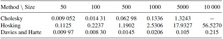
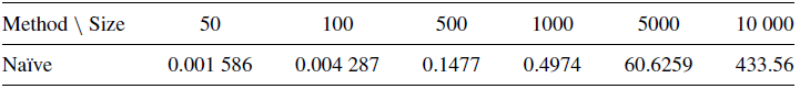


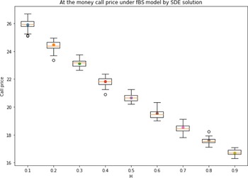


 Open access