2. Model

We develop a model for the flow of a buoyant incompressible current of density $\widehat {\rho _1}$ and viscosity $\hat {\mu }$ through a uniform porous medium of permeability $\hat {k}$ and porosity $\phi$. We define the depth below the crest of the upper surface of the anticline to be $\hat {b}(\hat {x})$ (see figure 2), where $\hat {x}$ is the lateral distance from the crest. Throughout the remainder of this paper we consider the case of a shallow incline $\hat {b}(\hat {x}) = \hat {x} \tan \theta$. The medium is initially saturated with ambient brine of density $\widehat {\rho _2}$. The fluid is injected by a line source along the crest of the anticline with injection flux per unit length $\hat {Q}$.

Figure 2. Outline of the flow of a buoyant plume of hydrogen of density $\hat {\rho }_1$, viscosity $\hat {\mu }$ and thickness $\hat {h}(\hat {x})$ in a porous medium of permeability $\hat {k}$, porosity $\phi$ and cap rock geometry described by $\hat {b}(\hat {x})$, traveling with horizontal speed $\hat {u}$. The coordinate system is shown with $\hat {x}$ and $\hat {y}$ denoting the horizontal and vertical axes respectively. The ambient brine present has density $\hat {\rho }_2$.

With a line source injection, the problem is two dimensional and it is appropriate to work in Cartesian coordinates. As a simplification, we consider the case in which the interface between the hydrogen and the water remains localised and we assume that the current lies in the region $0 < \hat {y} < \hat {h}(\hat {x},\hat {t})$ and $0 < \hat {x} < \hat {x}_f$, where $\hat {t}$ is time (figure 2). Here, $\hat {h}(\hat {x},\hat {t})$ is the thickness of the current while $\hat {x}_f$ is the horizontal position where the interface makes contact with the boundary, meaning $\hat {h}(\hat {x}_f, \hat {t}) = \hat {x}_f \tan \theta$. The flow is then described by Darcy's law in tandem with the incompressibility condition (Bear Reference Bear1988)

(2.1a,b)\begin{equation} \hat{\boldsymbol{u}} ={-} \frac{\hat{k}}{\hat{\mu}} ( \hat{\boldsymbol{\nabla}} \hat{p} - \hat{\rho} \hat{\boldsymbol{g}} ) \quad \text{and} \quad \hat{\boldsymbol{\nabla}} \boldsymbol{\cdot} \hat{\boldsymbol{u}} = 0, \end{equation}

where $\hat {p}(\hat {x},\hat {y})$ is the pressure at the point $(\hat {x},\hat {y})$.

In general the gravity current will spread out becoming long and thin $\hat {h} - \hat {b} \ll \hat {x}_f$, such that its horizontal extent is much larger than its vertical extent. From the incompressibility condition (2.1a,b), we can deduce

(2.2)\begin{equation} \hat{v} \sim \delta \hat{u} \sim 0,\quad \text{for }\delta \ll 1, \end{equation}

where $\delta$ is the ratio of the characteristic vertical to horizontal length scale. From relation (2.2), it can be seen that at long time the vertical component $\hat {v}$ of the velocity $\hat {\boldsymbol {u}}$ becomes negligible which then implies the pressure varies hydrostatically as given by

(2.3)\begin{equation} \hat{p}(\hat{x}, \hat{y}, \hat{t}) = \hat{P}_0(\hat{x}, \hat{t} ) - \Delta \hat{\rho} \hat{g} (\hat{h}(\hat{x}, \hat{t}) - \hat{y}) , \end{equation}

where $\Delta \hat {\rho } = \hat {\rho }_2 - \hat {\rho }_1$ and $\hat {P}_0( \hat {x}, \hat {t} )$ is the pressure at the fluid interface. When the aquifer has much greater depth than the thickness of the hydrogen plume, the pressure at the interface may be taken to be approximately constant (Pegler et al. Reference Pegler, Huppert and Neufeld2013)

(2.4)\begin{equation} \hat{p}(\hat{x}, \hat{y}, \hat{t}) = \hat{P}_0 - \Delta \hat{\rho} \hat{g} (\hat{h}(\hat{x}, \hat{t}) - \hat{y} ) . \end{equation}

With the pressure relation (2.4), we then determine the horizontal component of the velocity $\hat {u}$ to be

(2.5)\begin{equation} \hat{u} ={-} \hat{S} \frac{\partial \hat{h}}{\partial \hat{x}} , \end{equation}

where $\hat {S} = {\hat {k} \Delta \hat {\rho } \hat {g}}/{\hat {\mu }}$ is the buoyancy speed, which is the characteristic speed associated with a gravity current in a porous medium.

Local conservation of mass of the fluid is given by the equation

(2.6)\begin{equation} \phi \frac{\partial \hat{h}}{\partial \hat{t}} ={-} \frac{ \partial ( ( \hat{h} - \hat{x} \tan (\theta) ) \hat{u})}{\partial \hat{x}}. \end{equation}

Combining this with (2.5) we find

(2.7)\begin{equation} \phi \frac{\partial \hat{h}}{\partial \hat{t}} = \hat{S} \frac{\partial }{\partial \hat{x} } \biggl[(\hat{h} - \hat{x} \tan (\theta)) \frac{\partial \hat{h} }{\partial \hat{x}} \biggr] . \end{equation}

Volume conservation (per unit length) takes the form

(2.8)\begin{equation} \phi \int_0^{ \hat{x}_{f} } (\hat{h} - \hat{x} \tan \theta ) \, {\rm d} \hat{x} = \hat{V}(\hat{t} ) . \end{equation}

We also impose the condition $\hat {h}(\hat {x}_f, \hat {t}) = \hat {x}_f \tan \theta$ at the contact point. We assume the initial condition

(2.9)\begin{equation} \hat{h}(\hat{x}, 0) = \hat{x} \tan \theta . \end{equation}

We seek solutions to the governing equation (2.7) when there is a flux at $\hat {x}=0$ of the form (Dudfield & Woods Reference Dudfield and Woods2012)

(2.10) \begin{equation} \hat{Q} ={-} \hat{S} \hat{h} \left.\frac{\partial \hat{h} }{\partial \hat{x}}\right|_{\hat{x}=0} = \begin{cases} \hat{Q}_0 & \text{if } 2n {\rm \pi}\leq \hat{\omega} \hat{t} < (2n + 1) {\rm \pi}, \\ -\hat{Q}_0 & \text{if } (2n+1) {\rm \pi}\leq \hat{\omega} \hat{t} < (2n + 2) {\rm \pi}\text{ and } \hat{h}(0,\hat{t}) > 0, \\ 0 & \text{if } (2n+1) {\rm \pi}\leq \hat{\omega} \hat{t} < (2n + 2) {\rm \pi}\text{ and } \hat{h}(0,\hat{t}) = 0, \end{cases} \end{equation}

where $\hat {t}$ is time, $\hat {Q}_0$ is the characteristic scale of the injection flux per unit length along the well, $\hat {\omega }$ is a rate parameter which determines the frequency of oscillations and $n \geq 0$ is the cycle number.

It is instructive to consider the problem in dimensionless form. To this end we define the following dimensionless variables (Pegler et al. Reference Pegler, Huppert and Neufeld2013):

(2.11a–d)\begin{equation} x = \frac{ \tan^2(\theta) \hat{S}}{\hat{Q}_0} \hat{x} , \quad h = \frac{ \tan (\theta) \hat{S}}{\hat{Q}_0} \hat{h} , \quad t = \frac{ \tan^3 (\theta) \hat{S}^2}{\phi \hat{Q}_0} \hat{t} \quad \text{and} \quad Q = \frac{\hat{Q}}{\hat{Q}_0} . \end{equation}

The governing equation in non-dimensional form becomes

(2.12)\begin{equation} \frac{\partial h}{\partial t} = \frac{\partial }{\partial x } \left[ (h - x ) \frac{\partial h }{\partial x } \right] . \end{equation}

The flux condition at the source now has the form

(2.13)\begin{equation} Q ={-} h \left.\frac{\partial h }{\partial x} \right|_{x=0} = \begin{cases} 1 & \text{if } 2n {\rm \pi}\beta \leq t < (2n + 1) {\rm \pi}\beta ,\\ -1 & \text{if } (2n+1) {\rm \pi}\beta \leq t < (2n + 2) {\rm \pi}\beta \text{ and } h(0,t) > 0, \\ 0 & \text{if } (2n+1) {\rm \pi}\beta \leq t < (2n + 2) {\rm \pi}\beta \text{ and } h(0,t)= 0, \end{cases} \end{equation}

while

(2.14a,b)\begin{equation} h(x_f(t), t) = x_f(t) \quad \text{and} \quad h(x, 0) = x. \end{equation}

The dimensionless group $\beta$ given by

(2.15)\begin{equation} \beta = \frac{ \tan^3 (\theta) \hat{S}^2}{\phi \hat{Q}_0 \hat{\omega}} \end{equation}

measures the importance of the square of the buoyancy speed relative to the product of the injection rate and injection frequency. From relations (2.11a–d), it can be seen that for the current to be long and thin we require $\theta \ll 45^{\circ }$. During an extraction phase ($Q < 0$) the thickness of the current at the origin may decrease to zero, $h(0,t) = 0$. This is undesirable as in such a case, the formation fluid/brine will be produced at the extraction well. If this occurs we assume the extraction of fluid is stopped for the remainder of the cycle and then we begin injection again at the start of the next cycle. In the early cycles a mismatch develops whereby more fluid is injected than extracted over a cycle, resulting in a net increase in the volume of hydrogen in the porous medium. After successive injection and extraction cycles, there is sufficient net accumulation of hydrogen that a periodic cycle develops in which the volume of fluid extracted matches the volume of fluid injected. In the next section we study this equilibrium state and then we examine the initial transient filling of the system.

3. Equilibrium states

To study the equilibrium states described at the end of the last section, we solved the system (2.12)–(2.14a,b) numerically using a finite-volume scheme (Kurganov & Tadmor Reference Kurganov and Tadmor2000; Yu et al. Reference Yu, Zheng and Stone2017). The code is run until a periodic cycle develops which we define to develop when the fractional increase of the volume of hydrogen between successive cycles is less than $10^{-4}$.

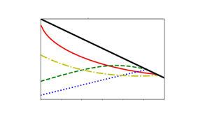
In figure 3, we illustrate the evolution of a hydrogen plume through a periodic cycle for five different values of $\beta$. Each plot shows the plume at four times through a cycle, namely at $t_e = 0$, ${{\rm \pi} \beta }/{2}$, ${\rm \pi} \beta$ and ${3 {\rm \pi}\beta }/{2}$, where the period of the cycle is $2 {\rm \pi}\beta$ and $t_e$ is the time during one injection–extraction cycle at equilibrium, meaning $0 \leq t_e < 2 {\rm \pi}\beta$. It is interesting to note that in plots (a) and (b) of figure 3, a region far from the source can be observed where the thickness of the plume changes very little over the course of an injection–extraction cycle (see figure 4). We define the point where this region begins to be $(x^*, h^*)$. However, for larger values of $\beta$ (see figure 3c–e), it can be seen that the entire interface, $h(x,t)$ in the region $0 \leq x \leq x_f$, oscillates significantly over the injection–extraction cycle. This is because as the parameter $\beta$ increases, the relative strength of the buoyancy speed with respect to the injection speed increases thus allowing fluid injected at the origin to be transmitted further across the porous medium during a single injection–extraction cycle. If $\beta$ is large enough then eventually these oscillations are transmitted far enough over a cycle that they reach the boundary at the leading edge of the current. We denote the critical value of $\beta$ for which this phenomenon occurs to be $\beta _c$.

Figure 3. The thickness of the plume $h$ plotted as a function of horizontal position $x$ at a series of times during an injection–extraction cycle once the systems has reached a quasi-equilibrium. Examples are given for five values of $\beta$: (a) $\beta = 0.001$; (b) $\beta = 0.01$; (c) $\beta = 0.25$; (d) $\beta = 1$; and (e) $\beta = 5$.

Figure 4. Two diagrams at different times during an injection–extraction cycle once equilibrium has been achieved showing an approximately time-independent region in the far-field. The point ($x^*, h^*$) denotes the beginning of this region. The point ($x_f, h_f$) is the contact point of the current and the boundary.

The value of $\beta _c$ may be approximated numerically by varying $\beta$ until there are noticeable oscillations at the leading edge of the current once equilibrium is reached. We define this to be when either the minimum or maximum value of the contact point $h_{min}$ or $h_{max}$ first differs from their average value $\bar {h}_f$ by $1\,\%$ during a cycle. We have determined the approximate value to be $\beta _c \approx 0.05$. Similarly, we can determine approximately the time independent region $(x^*, h^*)$ numerically by finding the closest lateral point to the source $x^*$, where the thickness $h^*$ differs by less than $1\,\%$ of the average thickness at the leading edge $\bar {h}_f$ during the entire cycle. When the difference is greater than $1\,\%$, $(x^*, h^*) = (\bar {x}_f, \bar {h}_f)$

To gain insight into how this far-field region depends on the parameter $\beta$, we can develop some scalings. First, consider the regime where the oscillations near the source do not reach the boundary over the course of a cycle and the approximately time-independent region in the far-field is present. Let $\hat {L}^*$ and $\hat {H}^*$ be the dimensional length and height scales associated with the oscillations during a cycle. The balance of mass over a cycle then requires that

(3.1)\begin{equation} \frac{\hat{Q}_{0}}{\hat{\omega}} \sim \phi \hat{L}^*\hat{H}^* , \end{equation}

where $\phi \hat {L}^*\hat {H}^*$ is a scaling for the volume associated with the oscillations. The flux in terms of $\hat {L}^*$ and $\hat {H}^*$ is given by

(3.2)\begin{equation} \hat{Q}_{0} \sim \biggl( \frac{\hat{S} \hat{H}^*}{\hat{L}^*} \biggr) \hat{H}^* . \end{equation}

Combining relations (3.1) and (3.2) we can determine scalings for both $\hat {H}^*$ and $\hat {L}^*$ finding

(3.3a,b)\begin{equation} \hat{H}^* \sim \biggl( \frac{\hat{Q}_{0}^2}{\phi \hat{S} \hat{\omega}} \biggr)^{{1}/{3}} \quad \text{and}\quad \hat{L}^* \sim \biggl( \frac{ \hat{S} \hat{Q}_{0}}{\phi \hat{\omega}^2} \biggr)^{{1}/{3}}. \end{equation}

Writing these scalings in non-dimensional form we find

(3.4a,b)\begin{equation} h^* \sim \beta^{{1}/{3}} \quad \text{and} \quad x^* \sim \beta^{{2}/{3}}. \end{equation}

These scalings show that as $\beta$ takes progressively smaller values, the flow becomes more localised near the well, and eventually the approximation of a long and thin one-dimensional flow ceases to apply.

Since the height of the time-independent region in the far-field is approximately the same as the height at the leading edge we deduce $h^* \approx h_f$ due to the time-independent approximation in the far-field, and $x_f = h_f$ due to the linear inclination of the cap-rock, thus

(3.5a,b)\begin{equation} h_f \sim \beta^{{1}/{3}} \quad \text{and}\quad x_f \sim \beta^{{1}/{3}} . \end{equation}

Note from relation (3.5a,b) we see the total volume in the system obeys the following power law:

(3.6)\begin{equation} V \sim \beta^{{2}/{3}}. \end{equation}

In the second equilibrium regime, when the oscillations propagate across the entire interface the flow is constrained by the boundary, $\hat {L}^* \ \tan \theta \sim \hat {H}^*$. This implies that $x^* \sim x_f$. We now expect

(3.7)\begin{equation} x^* \sim \beta^{{1}/{3}} . \end{equation}

The corresponding scalings for $h_f$, $x_f$, $h^*$ and $V$ do not change from relations (3.4a,b)–(3.6) in this regime.

To test the validity of these scalings in figure 5, we show the variation of $\log (\bar {h}_f)$ (a), $\log (\bar {V})$ (b) and $\log (x^*)$ (c) as functions of $\log \beta$. Here $\bar {V}$ is the average of the maximum and minimum volume values during an injection–extraction cycle at equilibrium. In (a,b) the linearity of the curves implies that $\bar {h}_f$ and $\bar {V}$ grow consistent with relations (3.5a,b) and (3.6), respectively. In (c), linearity again implies power laws are followed whereby the far-field region beginning at $x^*$ initially grows as $\beta ^{{2}/{3}}$. However, once the oscillations reach the edge of the current denoted by the vertical dotted line in (c), $x^* \approx x_f$ and $x^*$ then grows as $\beta ^{{1}/{3}}$. These results are consistent with the scalings derived in relations (3.4a,b)–(3.7). Lines of best fit are illustrated in each plot by dashed black lines with coefficients given in the caption. As mentioned earlier once an equilibrium state has been reached the volume injected $V_w$ matches the volume extracted. We define the working fraction $W_f$ as the ratio of the volume of working gas $V_w$ to the sum of the working gas and cushion gas $V_c$:

(3.8)\begin{equation} W_f = \frac{V_w}{ V_w + V_c } , \end{equation}

where the cushion gas $V_c$ is the volume of fluid that cannot be recovered during the extraction phase (Heinemann et al. Reference Heinemann, Scafidi, Pickup, Thaysen, Hassanpouryouzband, Wilkinson, Satterley, Booth, Edlmann and Haszeldine2021b). Knowledge of how the working fraction $W_f$ varies as a function of $\beta$ is important. In figure 6 we plot the working fraction $W_f$ as a function of $\log \beta$. The larger-amplitude oscillations along the fluid interface lead to a larger volume of fluid being injected and extracted in each cycle. This results in a higher working fraction. Note that the increase of $\beta$ resulting in larger working fractions implies that steepening the incline increases the working fraction. This is because of the greater constraint on the lateral extent $x_f$ of the current causing greater localisation of the hydrogen plume around the source.

Figure 5. ${\rm Log}$–$\log$ plots of $\bar {h}_f$ (a), $\bar {V}$ (b) and $x^*$ (c), as functions of varying $\beta$ (red circles). The lines of best fit (dashed black lines) are $\log \bar {h}_f = 0.34 \log \beta + 0.76$, $\log \bar {V} = 0.67 \log \beta + 0.74$, $\log x^* = 0.63 \log \beta + 1.70$ ($\beta < \beta _c$) and $\log x^* = 0.35 \log \beta + 0.79$ ($\beta > \beta _c$). The vertical dotted blue line in (c) denotes $\log \beta = \log \beta _c$. The slopes of the solid black lines indicate the theoretical predictions given by (3.4a,b)–(3.7).

Figure 6. The working fraction $W_f$ plotted as a function of varying $\log \beta$.

4. Initial transient regime

Before an equilibrium state is reached the current is in a transient state where a net increase in the volume flow of fluid occurs across a cycle due to the mismatch between the amount of fluid injected and extracted. This is because in our model if the thickness of the current at the source becomes zero, extraction is stopped to prevent brine production at the well. To understand how the parameter $\beta$ effects this transient regime, in figure 7 we show how the volume $V$ varies with time for five values of $\beta$ as the current reaches equilibrium. It can be seen that for larger values of $\beta$ the number of cycles needed to reach equilibrium decreases. This is due to the greater buoyancy speed which transmits fluid further into the far field and results in less localisation of fluid around the source. In turn, this causes a greater net in-flow across each cycle. As a result, the current can be supplied with the required amount of fluid to reach equilibrium over a smaller number of cycles.

Figure 7. Volume of fluid $V$ plotted as a function of varying time $t$, for five values of $\beta$: (a) $\beta = 0.001$, (b) $\beta = 0.01$, (c) $\beta = 0.25$, (d) $\beta = 1$ and (e) $\beta = 5$. The working and cushion gas volumes have been denoted in (c).

To see systematically how the number of injection–extraction cycles depends on the dimensionless parameter $\beta$, in figure 8 we present a $\log \unicode{x2013}\log$ plot of the number of injection–extraction cycles $n$ required to achieve equilibrium as a function of varying $\log \beta$. The number of cycles required to reach equilibrium $n$ rapidly decays with $\beta$ due to the greater amount of fluid injected in each cycle. Curiously this plot suggests that the number of cycles decays as a power law in $\beta$,

(4.1)\begin{equation} n \sim \beta^{-{1}/{2}} . \end{equation}

Given that each cycle persists for a dimensionless time $2 {\rm \pi}\beta$, this implies that the time to reach equilibrium scales as

(4.2)\begin{equation} t_s \sim \beta n \sim \beta^{{1}/{2}}. \end{equation}

Figure 8. A $\log \unicode{x2013}\log$ plot of the number of injection–extraction cycles required to achieve equilibrium $n$ plotted as a function of varying $\beta$ (red circles). The black dashed line is the line of best fit: $\log n = -0.50 \log \beta + 1.33$.

In the case that $\beta$ is small, there are a significant number of cycles required to reach equilibrium. Given the clear scaling laws for the total volume injected, $\beta ^{{2}/{3}}$, and the number of cycles needed to reach equilibrium, (4.1), we now explore whether there is a law for how the net flux over a cycle decays as a function of the cycle number scaled with the total number of cycles required for the system to equilibrate. If we divide the total volume $\beta ^{{2}/{3}}$ (3.6) by the power law for the total number of cycles (4.1) we find a scaling for the flux per cycle. We then hypothesise that the net volume injected depends on the time at the end of the $i$th cycle, $t_i = 2{\rm \pi} \beta i$, scaled by the timescale to reach equilibrium, $\beta ^{1/2}$ according to a dimensionless function $f(t_i / \beta ^{1/2})$, which we assume decays to zero as $i \rightarrow n$, and where cycle $i$ occurs over the time interval $2{\rm \pi} \beta (i-1) < t < 2 {\rm \pi}\beta i$. This suggests that the injected volume on cycle $i$, $V^{{i}}_{{m}}$, as a function of $\beta$ might follow a scaling law of the form:

(4.3)\begin{equation} V^{{i}}_{{m}} \sim {\beta^{{7}/{6}}} {f( \beta^{1/2} i)} . \end{equation}

In figure 9, we now compare the relation (4.3) with the numerical data: to this end, we plot curves of the scaled net volume addition $V^{{i}}_{{m}}/\beta ^{7/6}$ as a function of $t_i/\beta ^{1/2}$. Curves are given for several values of $\beta$ spanning several orders of magnitude, on both linear and logarithmic axes. The figure suggests that, to leading order, the scaled numerical data do seem follow a similar trend line, although we note that there is some scatter in the data.

Figure 9. (a) Plot of $V_m \beta ^{-{7}/{6}}$ as a function of varying $t \beta ^{-{1}/{2}}$ for four values of $\beta$. The corresponding $\log \unicode{x2013}\log$ plot is presented in (b).