


1. Introduction
Large-scale planetary (Rossby) waves are observed at the low and mid latitudes over much of the world ocean (Kessler Reference Kessler1990; Chelton & Schlax Reference Chelton and Schlax1996; Zang & Wunsch Reference Zang and Wunsch1999; Cipollini et al. Reference Cipollini, Cromwell, Challenor and Raffaglio2001; Osychny & Cornillon Reference Osychny and Cornillon2004; Jury Reference Jury2018). The waves were first predicted by Rossby (Rossby Reference Rossby1939; Platzman Reference Platzman1968; Madden Reference Madden1979) and are routinely invoked in atmospheric dynamics, for instance with respect to ‘teleconnections’ (Ambrizzi, Hoskins & Hsu Reference Ambrizzi, Hoskins and Hsu1995; Galanti & Tziperman Reference Galanti and Tziperman2003; Rivière Reference Rivière2010; Tseng, Maloney & Barnes Reference Tseng, Maloney and Barnes2019). Rossby waves exist because of the beta effect – the meridional gradient of the Coriolis parameter (which increases monotonically with latitude). Because of
 $\beta$
, meridional motion alters the vorticity on fluid parcels, and the resulting restoring force supports waves.
$\beta$
, meridional motion alters the vorticity on fluid parcels, and the resulting restoring force supports waves.
In the ocean, Rossby waves are seen clearly in satellite observations of sea surface height. These are primarily ‘baroclinic’ Rossby waves, which have vertical shear and longer time scales than unsheared ‘barotropic’ waves. A signature of the baroclinic waves is westward phase propagation, with a phase speed that is largest at the equator and decreasing towards the poles. Such propagation is seen in all major ocean basins, outside boundary currents like the Gulf Stream and the Antarctic Circumpolar Current. In the tropics (20S to 20N), the waves are large, exceeding thousands of kilometres, but they are smaller at higher latitudes, closer to the internal ‘deformation scale’ (typically tens of kilometres). Furthermore, at mid and high latitudes, the waves are more nonlinear, exhibiting meridional propagation as well; cyclones are deflected to the north-west, and anticyclones to the south-west (Chelton, Schlax & Samelson Reference Chelton, Schlax and Samelson2011).
The phase speed at low latitudes is comparable to the theoretical long wave speed for traditional, first baroclinic mode Rossby waves, the gravest of the vertically sheared modes (Chelton & Schlax Reference Chelton and Schlax1996). However, the speeds outside the 20S–20N range are consistently faster than predicted – in some cases twice as fast. A number of explanations have been proposed, but the most likely is that the waves are modified over a rough bottom (Samelson Reference Samelson1992; Bobrovich & Reznik Reference Bobrovich and Reznik1999; Reznik & Tsybaneva Reference Reznik and Tsybaneva1999; Vanneste Reference Vanneste2000; Tailleux & McWilliams Reference Tailleux and McWilliams2001; LaCasce Reference LaCasce2017; Clarke & Buchanan Reference Clarke and Buchanan2024; Davis et al. Reference Davis, Radko, Brown and Dewar2025). Over steep topography, the baroclinic modes have nearly zero flow at the bottom and a larger deformation radius; as the long wave phase speed is proportional to the deformation radius squared, the waves are faster (LaCasce & Groeskamp Reference LaCasce and Groeskamp2020). Current meter observations suggest that such ‘rough bottom modes’ are common in the ocean (de La Lama et al. Reference de La Lama, LaCasce and Fuhr2016).
Less attention has been paid to the change in the lateral scale of the waves, from large structures at low latitudes to deformation scale, vortex-like features at higher latitudes. One proposed explanation is that a turbulent inverse energy cascade transitions to Rossby waves at different scales, due to the latitudinal variation of
 $\beta$
(Theiss Reference Theiss2004). Another explanation is that the Rossby waves are unstable. This instability has been explored in the barotropic context (Lorenz Reference Lorenz1972; Gill Reference Gill1974) and the baroclinic one (Jones Reference Jones1978, Reference Jones1979; Vanneste Reference Vanneste1995; LaCasce & Pedlosky Reference LaCasce and Pedlosky2004). Originating at the eastern boundary, the wave crests are oriented approximately north–south, and as such, shear instability cannot be stabilised by
$\beta$
(Theiss Reference Theiss2004). Another explanation is that the Rossby waves are unstable. This instability has been explored in the barotropic context (Lorenz Reference Lorenz1972; Gill Reference Gill1974) and the baroclinic one (Jones Reference Jones1978, Reference Jones1979; Vanneste Reference Vanneste1995; LaCasce & Pedlosky Reference LaCasce and Pedlosky2004). Originating at the eastern boundary, the wave crests are oriented approximately north–south, and as such, shear instability cannot be stabilised by
 $\beta$
(Kamenkovich & Pedlosky Reference Kamenkovich and Pedlosky1996).
$\beta$
(Kamenkovich & Pedlosky Reference Kamenkovich and Pedlosky1996).
The question then is how far the waves propagate into the interior before breaking into smaller eddies. At low latitudes, the waves move faster and cross the basin intact, but the slower waves at higher latitudes succumb before crossing. The difference can be quantified by a parameter
 $Z$
defined by
$Z$
defined by
 \begin{equation} Z = \frac {T_c}{T_g} = \frac {U L_b}{\beta L_{d1}^3} \;, \end{equation}
i.e. the ratio of the crossing time to the unstable growth time (LaCasce & Pedlosky (Reference LaCasce and Pedlosky2004), LP04 hereafter). Here,
 $L_b$
is the basin scale, and
$L_b$
is the basin scale, and
 $L_{d1}$
is the first baroclinic deformation radius, while
$L_{d1}$
is the first baroclinic deformation radius, while
 $\beta$
is the meridional gradient of the Coriolis parameter (
$\beta$
is the meridional gradient of the Coriolis parameter (
 $f$
), and
$f$
), and
 $U$
is a velocity scale. As the deformation radius is inversely proportional to
$U$
is a velocity scale. As the deformation radius is inversely proportional to
 $f$
,
$f$
,
 $Z$
increases rapidly with latitude. It is near unity at
$Z$
increases rapidly with latitude. It is near unity at
 $20^\circ$
, in line with observations that smaller scale eddies dominate outside the range 20S–20N. LP04 employed quasi-geostrophic (QG) dynamics, but consistent results are obtained under the full primitive equations (Isachsen, LaCasce & Pedlosky Reference Isachsen, LaCasce and Pedlosky2007).
$20^\circ$
, in line with observations that smaller scale eddies dominate outside the range 20S–20N. LP04 employed quasi-geostrophic (QG) dynamics, but consistent results are obtained under the full primitive equations (Isachsen, LaCasce & Pedlosky Reference Isachsen, LaCasce and Pedlosky2007).
However, these previous studies were conducted with a flat bottom. The results could well vary with bottom roughness, which affects baroclinic instability (De Szoeke Reference De Szoeke1983; Benilov Reference Benilov2001; Vanneste Reference Vanneste2003; LaCasce et al. Reference LaCasce, Escartin, Chassignet and Xu2019; Radko Reference Radko2019; Davies, Khatri & Berloff Reference Davies, Khatri and Berloff2021; Palóczy & LaCasce Reference Palóczy and LaCasce2022). One-dimensional ridges are particularly effective in this regard, suppressing deep motion perpendicular to the ridges, but suppression occurs as well with two-dimensional relief. Topography impacts the growth rates and scales of the resulting eddies, and in turbulent flows can scatter energy to both smaller and larger scales (Rhines Reference Rhines1977; Owens & Bretherton Reference Owens and Bretherton1978; Treguier & Hua Reference Treguier and Hua1988; Treguier & McWilliams Reference Treguier and McWilliams1990; Palóczy & LaCasce Reference Palóczy and LaCasce2022; Zhang & Xie Reference Zhang and Xie2024; Pudig & Smith Reference Pudig and Smith2025).
Hereafter, we examine how two-dimensional relief affects Rossby wave stability and characteristics. Rossby waves have lateral shear and are time dependent, so we employ simplified dynamics (two fluid layers, the QG approximation and sinusoidal bathymetry). As will be seen, topography does not inhibit the instability of large waves, so the predicted latitudinal dependence should be unaltered from LP04. But if the topographic height exceeds a critical value, then the unstable growth is essentially locked to the bathymetry. Then the growth rate is independent of topographic height, and the horizontal scale of the resultant eddies is determined by topography. As such, the instability is significantly different over a flat bottom.
The equations are presented in § 2. Nonlinear simulations in a basin, similar to those by LP04, are discussed in § 3, and the linear stability calculations in § 4. In § 5, the presented theory is applied to Earth’s oceans. The results are summarised and discussed thereafter.
2. The QG equations
We employ the two-layer QG potential vorticity (PV) equations. The QG approximation, which assumes hydrostatic balance and a small Rossby number, is reasonable for synoptic-scale oceanic applications (Pedlosky Reference Pedlosky1979; Vallis Reference Vallis2017). The unknowns are the geostrophic streamfunctions in the upper and lower layers,
 $\psi _1$
and
$\psi _1$
and
 $\psi _2$
. These are related to the PV in the corresponding layers via
$\psi _2$
. These are related to the PV in the corresponding layers via
 \begin{equation} q_i = {\nabla} ^2 \psi _i + F_i \left ( \psi _{3-i} -\psi _i\right ), \end{equation}
where
 $F_i = L^2/L_{di}^2 = f_0^2 L^2/(g' H_i)$
are inverse Burgers numbers. Here,
$F_i = L^2/L_{di}^2 = f_0^2 L^2/(g' H_i)$
are inverse Burgers numbers. Here,
 $f_0$
is the mean Coriolis parameter,
$f_0$
is the mean Coriolis parameter,
 $g'=(\rho _2 - \rho _1)g/\rho _c$
is the reduced gravity (where
$g'=(\rho _2 - \rho _1)g/\rho _c$
is the reduced gravity (where
 $\rho _c$
is the mean of the layer densities), and
$\rho _c$
is the mean of the layer densities), and
 $H_i$
is the depth of the
$H_i$
is the depth of the
 $i$
th layer at rest. The parameter
$i$
th layer at rest. The parameter
 $L$
is the domain scale, such that the model basin has dimensions
$L$
is the domain scale, such that the model basin has dimensions
 $\pi \times \pi$
.
$\pi \times \pi$
.
In the absence of external forcing or damping, the PV evolves following (Pedlosky Reference Pedlosky1979; Vallis Reference Vallis2017)
 \begin{align} &\hspace{2.5pc} {\frac {\partial q_1}{\partial t}} + J(\psi _1,q_1) + \beta {\frac {\partial \psi _1}{\partial x}} = D_1, \end{align}
 \begin{align} &{\frac {\partial q_2}{\partial t}} + J(\psi _2,q_2) + \beta {\frac {\partial \psi _2}{\partial x}} + J(\psi _2,h) = D_2 , \end{align}
where
 $J({\cdot },{\cdot })$
is the Jacobian operator, and the
$J({\cdot },{\cdot })$
is the Jacobian operator, and the
 $D_i$
represent small-scale dissipation. There are two parameters that determine the response. The first is the (scaled) meridional gradient of the Coriolis parameter:
$D_i$
represent small-scale dissipation. There are two parameters that determine the response. The first is the (scaled) meridional gradient of the Coriolis parameter:
 \begin{equation} \beta \equiv \frac {\beta _d L^2}{U} , \end{equation}
where
 $\beta _d$
is the dimensional gradient, and
$\beta _d$
is the dimensional gradient, and
 $U$
is the velocity scale of the wave. With a large
$U$
is the velocity scale of the wave. With a large
 $\beta$
, the dynamics are wave-like to first order, as in the small-
$\beta$
, the dynamics are wave-like to first order, as in the small-
 $Z$
limit of LP04 (1.1).
$Z$
limit of LP04 (1.1).
The other parameter is the non-dimensional topographic height:
 \begin{equation} h \equiv \frac {f_0 L h_d}{U H} = \frac {1}{R_o} \frac {h_d}{H} . \end{equation}
Here,
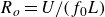 $R_o=U/(f_0 L)$
is the Rossby number based on the domain scale, and
$R_o=U/(f_0 L)$
is the Rossby number based on the domain scale, and
 $H=H_1+H_2$
is the total depth. We have assumed that the topography has a scale comparable to that of the domain; this is relaxed later. If the latter is 1000 km, then
$H=H_1+H_2$
is the total depth. We have assumed that the topography has a scale comparable to that of the domain; this is relaxed later. If the latter is 1000 km, then
 $R_o \approx 10^{-3}$
. If the depth is of order 1000 m, as in the ocean interior, the non-dimensional topographic height translates approximately to metres:
$R_o \approx 10^{-3}$
. If the depth is of order 1000 m, as in the ocean interior, the non-dimensional topographic height translates approximately to metres:
 $h=1$
indicates dimensional height
$h=1$
indicates dimensional height
 $h_d \approx 1$
m.
$h_d \approx 1$
m.
Hereafter, we fix the layer depth ratio at
 $1/4$
:
$1/4$
:
 \begin{align} \delta \equiv \frac {\delta _1}{\delta _2} = \frac {H_1/H}{H_2/H} = \frac 14. \end{align}
This mimics the density stratification in the ocean interior. For the inverse Burgers number, a value
 $F_1=500$
implies that the basin size is 22.4 times the surface deformation radius. The latter is of order 30–40 km at mid latitudes (LaCasce & Groeskamp Reference LaCasce and Groeskamp2020).
$F_1=500$
implies that the basin size is 22.4 times the surface deformation radius. The latter is of order 30–40 km at mid latitudes (LaCasce & Groeskamp Reference LaCasce and Groeskamp2020).
Under the PV equations, the total energy, the sum of the layer kinetic energies and the potential energy, is conserved in the absence of dissipation. The constituents are defined as
 \begin{equation} \textit{KE}_i = \frac {\delta _i}{2} \iint |\boldsymbol{\nabla }\psi _i|^2 \,{\rm d}A, \quad \textit{PE} = F \iint | \psi _1 - \psi _2 |^2 \,{\rm d}A. \end{equation}
The pre-factor of the potential energy is
 $F=\delta _1 F_1 = \delta _2 F_2$
.
$F=\delta _1 F_1 = \delta _2 F_2$
.
We employ two numerical models. The first is a nonlinear, two-layer basin code with topography; the second is a numerical linear stability routine. We present the models and the corresponding results in the respective sections.
3. Semi-spectral model
3.1. Model and initial condition
The nonlinear model solves (2.2)–(2.3) in a bounded square domain using finite differences (LaCasce Reference LaCasce2002; LaCasce & Pedlosky Reference LaCasce and Pedlosky2004; Brændshøi Reference Brændshøi2018). The model has a rigid upper surface and permits variable bottom relief. The model employs third-order Adams–Bashforth time stepping, and the PV (2.1) is inverted for the streamfunctions using sine transforms. The advective (Jacobian) terms are calculated using the third-order QUICK scheme of Leonard (Reference Leonard1979). This method introduces implicit (hyperdiffusive) dissipation that preferentially damps the small scales (e.g. Becker & Salmon Reference Becker and Salmon1997). The effective diffusivity is proportional to the flow speed and is a sensitive function of the grid spacing (to the third power). While convenient in some respects, for instance with regards to flow parallel to the walls, it does result in a degree of eddy damping, as seen hereafter.
The model is formulated in terms of barotropic and baroclinic modes defined by
 \begin{align} \psi _B = \delta _1 \psi _1 + \delta _2 \psi _2, \quad \psi _T = \psi _1 - \psi _2, \end{align}
respectively. This facilitates the PV inversions. All runs with this model use
 $512\times 512$
resolution.
$512\times 512$
resolution.
A significant issue is the boundary condition for the baroclinic streamfunction
 $\psi _T$
. Both streamfunctions are constant along the walls, to ensure no-normal flow. For the barotropic mode, this constant can be assumed to be zero, due to the rigid lid, but the baroclinic streamfunction is non-zero and can vary in time (Flierl Reference Flierl1977; McWilliams Reference McWilliams1977; LaCasce Reference LaCasce and Brink2000). Thus we introduce an additional variable
$\psi _T$
. Both streamfunctions are constant along the walls, to ensure no-normal flow. For the barotropic mode, this constant can be assumed to be zero, due to the rigid lid, but the baroclinic streamfunction is non-zero and can vary in time (Flierl Reference Flierl1977; McWilliams Reference McWilliams1977; LaCasce Reference LaCasce and Brink2000). Thus we introduce an additional variable
 $\varGamma (t)$
, the value of
$\varGamma (t)$
, the value of
 $\psi _T$
on the boundary; this is determined at each time step by imposing conservation of mass. Allowing
$\psi _T$
on the boundary; this is determined at each time step by imposing conservation of mass. Allowing
 $\varGamma$
to vary in time is equivalent to letting the layer interface move up and down on the boundaries. This is the model’s representation of Kelvin waves, which are infinitely fast under the QG approximation.
$\varGamma$
to vary in time is equivalent to letting the layer interface move up and down on the boundaries. This is the model’s representation of Kelvin waves, which are infinitely fast under the QG approximation.
For the initial condition, we assume a surface-trapped Rossby wave:
 \begin{equation} \psi _1= \sin (k_wx) \sin (y),\quad \psi _2=0, \end{equation}
where the wavenumber is
 $k_w=n \pi /L_x$
, to ensure an integral number of wavelengths in the domain. Note that the initial wave differs from that of LP04, which was purely baroclinic. As noted, a surface wave is more consistent with observations (de La Lama et al. Reference de La Lama, LaCasce and Fuhr2016). Using a surface wave also avoids a direct interaction with the bathymetry initially (although a surface-trapped wave will generate flow in the lower layer because of interfacial motion, as seen below). In many of the simulations, we fix
$k_w=n \pi /L_x$
, to ensure an integral number of wavelengths in the domain. Note that the initial wave differs from that of LP04, which was purely baroclinic. As noted, a surface wave is more consistent with observations (de La Lama et al. Reference de La Lama, LaCasce and Fuhr2016). Using a surface wave also avoids a direct interaction with the bathymetry initially (although a surface-trapped wave will generate flow in the lower layer because of interfacial motion, as seen below). In many of the simulations, we fix
 $F_1=500$
, corresponding to a deformation wavenumber
$F_1=500$
, corresponding to a deformation wavenumber
 $K_{d1}=22.4$
.
$K_{d1}=22.4$
.
We employ two types of bathymetry (e.g. Palóczy & LaCasce Reference Palóczy and LaCasce2022). One is a two-dimensional random field with a narrow-band spectrum (e.g. Constantinou Reference Constantinou2015; He & Wang Reference He and Wang2024; Pudig & Smith Reference Pudig and Smith2025). The second is an isotropic, monochromatic function:
 \begin{equation} h=h_0 \cos (k_t x) \cos (l_t y). \end{equation}
The results with both are consistent, but the topographic influence is more easily discerned when using monochromatic bathymetry. We set
 $k_t=l_t=p$
, with
$k_t=l_t=p$
, with
 $p=8$
or
$p=8$
or
 $10$
. As such, the topographic scale exceeds the surface deformation scale, with
$10$
. As such, the topographic scale exceeds the surface deformation scale, with
 $K_{d1}/K_t=1.6{-}2$
. We will focus on the response to different amplitudes
$K_{d1}/K_t=1.6{-}2$
. We will focus on the response to different amplitudes
 $h_0$
, and return to the random bathymetry when considering stability.
$h_0$
, and return to the random bathymetry when considering stability.
3.2. Results
For context, consider the response with a flat bottom (
 $h=0$
). An example with
$h=0$
). An example with
 $\beta =0.1$
is shown in figure 1. The small value of
$\beta =0.1$
is shown in figure 1. The small value of
 $\beta$
corresponds to a large
$\beta$
corresponds to a large
 $Z$
in (1.1), implying that the wave moves little over the time scale for unstable growth (as at mid latitudes). The solution with a larger
$Z$
in (1.1), implying that the wave moves little over the time scale for unstable growth (as at mid latitudes). The solution with a larger
 $\beta$
is qualitatively similar, except that the waves move across the basin while breaking down.
$\beta$
is qualitatively similar, except that the waves move across the basin while breaking down.
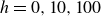
Flat bottom results for
 $F_1=500$
and
$F_1=500$
and
 $\beta =0.1$
. Upper row: the colour fields are the surface streamfunction
$\beta =0.1$
. Upper row: the colour fields are the surface streamfunction
 $\psi _1$
, while the white contours are the surface PV,
$\psi _1$
, while the white contours are the surface PV,
 $q_1$
. Bottom row: the upper-layer two-dimensional kinetic energy spectra at the same times.
$q_1$
. Bottom row: the upper-layer two-dimensional kinetic energy spectra at the same times.

The wave crests and troughs twist initially under mutual advection (figure 1
a); this is because the waves have a sinusoidal dependence on
 $y$
(as opposed to the nearly meridionally invariant profile used by LP04). The waves then break up into deformation scale eddies. These subsequently merge, yielding an inverse energy cascade (figure 1
c). Vortices are seen as well at late times, but the flow is dominated by two large gyres, anticyclonic in the north, and cyclonic in the south. These ‘Fofonoff gyres’ (Fofonoff Reference Fofonoff1955; Marshall & Nurser Reference Marshall and Nurser1986) are often observed in simulations of two-dimensional turbulence in a basin (Griffa & Salmon Reference Griffa and Salmon1989; Cummins Reference Cummins1992; Wang & Vallis Reference Wang and Vallis1994; LaCasce Reference LaCasce2002). The lower-layer streamfunctions (not shown) are very similar to those in the upper layer, as expected for barotropic flow. Indeed, there is a significant vertical transfer of energy (as the initial condition is surface-trapped).
$y$
(as opposed to the nearly meridionally invariant profile used by LP04). The waves then break up into deformation scale eddies. These subsequently merge, yielding an inverse energy cascade (figure 1
c). Vortices are seen as well at late times, but the flow is dominated by two large gyres, anticyclonic in the north, and cyclonic in the south. These ‘Fofonoff gyres’ (Fofonoff Reference Fofonoff1955; Marshall & Nurser Reference Marshall and Nurser1986) are often observed in simulations of two-dimensional turbulence in a basin (Griffa & Salmon Reference Griffa and Salmon1989; Cummins Reference Cummins1992; Wang & Vallis Reference Wang and Vallis1994; LaCasce Reference LaCasce2002). The lower-layer streamfunctions (not shown) are very similar to those in the upper layer, as expected for barotropic flow. Indeed, there is a significant vertical transfer of energy (as the initial condition is surface-trapped).
The essential elements of the evolution are captured by two-dimensional wavenumber spectra for the layer kinetic energies, shown in the lower panels of figure 1 for the surface energy. Here,
 \begin{equation} \widehat{\textit{KE}}_1(k,l) = \frac {\delta _1}{2} K^2\, |\hat \psi _1|^2, \end{equation}
where the hat indicates the Fourier transform, and
 $K=\sqrt {k^2+l^2}$
is the magnitude of the horizontal wavenumber. Initially, the spectrum reflects the wave, with
$K=\sqrt {k^2+l^2}$
is the magnitude of the horizontal wavenumber. Initially, the spectrum reflects the wave, with
 $k=k_w=4$
and
$k=k_w=4$
and
 $l\approx 0$
. By
$l\approx 0$
. By
 $t=1.875$
, the spectrum is more isotropic (figure 1
c), due to the baroclinic eddies. The dominant wavenumber is
$t=1.875$
, the spectrum is more isotropic (figure 1
c), due to the baroclinic eddies. The dominant wavenumber is
 $K\approx 8$
, somewhat less than
$K\approx 8$
, somewhat less than
 $\sqrt {F}=\sqrt {\delta _1 F_1}=10$
. Eventually, the energy is concentrated near
$\sqrt {F}=\sqrt {\delta _1 F_1}=10$
. Eventually, the energy is concentrated near
 $(k,l)\approx (0,2)$
, reflecting the Fofonoff gyres. The plots for
$(k,l)\approx (0,2)$
, reflecting the Fofonoff gyres. The plots for
 $\widehat{\textit{KE}}_2(k,l)$
are similar, as the late-time flow is nearly barotropic.
$\widehat{\textit{KE}}_2(k,l)$
are similar, as the late-time flow is nearly barotropic.
This evolution is as described by LP04, allowing for minor differences due to the choice of initial wave. With small-amplitude topography (
 $h\lt 1$
), the evolution is similar to that with a flat bottom. The primary difference is that the energy at late times, still predominantly near
$h\lt 1$
), the evolution is similar to that with a flat bottom. The primary difference is that the energy at late times, still predominantly near
 $k=0$
, is spread over more meridional wavenumbers (not shown). This is due to topographic perturbations of the Fofonoff gyres.
$k=0$
, is spread over more meridional wavenumbers (not shown). This is due to topographic perturbations of the Fofonoff gyres.
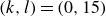
With larger heights, topographic effects are more pronounced. The case with
 $h=10$
(i.e. 10 m bumps) is shown in figure 2. Instability proceeds initially as in the flat bottom case (figure 2
a), with the primary wave becoming unstable and generating smaller-scale eddies. Indeed, the topographic influence is not obvious in the streamfunctions (upper panels of figures 2
b,c), but it is seen in the spectra, with a peak at
$h=10$
(i.e. 10 m bumps) is shown in figure 2. Instability proceeds initially as in the flat bottom case (figure 2
a), with the primary wave becoming unstable and generating smaller-scale eddies. Indeed, the topographic influence is not obvious in the streamfunctions (upper panels of figures 2
b,c), but it is seen in the spectra, with a peak at
 $(k,l)=(10,10)$
, the topographic wavenumbers. Nevertheless, the large-scale wave is still evident in animations, propagating westwards (not shown), and the system eventually evolves to Fofonoff gyres (figure 2
d). But the streamfunction reveals the topography as well, and both gyres and topographic-scale eddies are present. As before, the lower-layer streamfunction is similar since the baroclinic eddies are strongly barotropic.
$(k,l)=(10,10)$
, the topographic wavenumbers. Nevertheless, the large-scale wave is still evident in animations, propagating westwards (not shown), and the system eventually evolves to Fofonoff gyres (figure 2
d). But the streamfunction reveals the topography as well, and both gyres and topographic-scale eddies are present. As before, the lower-layer streamfunction is similar since the baroclinic eddies are strongly barotropic.
As in figure 1 but with moderate-amplitude topography (
 $h_0=10$
).
$h_0=10$
).

An example with higher topography (
 $h=100$
) is shown in figure 3. Note that the corresponding dimensional value is approximately 100 m in the ocean interior, which is less than 10 % of the total water depth, in line with the QG approximation. Compared to the
$h=100$
) is shown in figure 3. Note that the corresponding dimensional value is approximately 100 m in the ocean interior, which is less than 10 % of the total water depth, in line with the QG approximation. Compared to the
 $h=10$
case, wave instability proceeds more slowly; compare figures 3(b,c) with figures 2(b,c). Eventually, the wave does break up, but the Fofonoff gyres are absent at late stages (figure 3
d). Rather, the flow is locked to the bathymetry. The spectra confirm this, with a single peak at
$h=10$
case, wave instability proceeds more slowly; compare figures 3(b,c) with figures 2(b,c). Eventually, the wave does break up, but the Fofonoff gyres are absent at late stages (figure 3
d). Rather, the flow is locked to the bathymetry. The spectra confirm this, with a single peak at
 $(k,l)=(10,10)$
. The final state is thus very different to that over a flat bottom.
$(k,l)=(10,10)$
. The final state is thus very different to that over a flat bottom.
As in figure 1 but with large-amplitude topography (
 $h_0=100$
).
$h_0=100$
).

Despite the differences, the energetics evolve similarly in the three cases (figure 4). This is due primarily to the large value of
 $F_1$
, which ensures that the base wave’s potential energy is large. But topography induces secondary changes. With moderate bathymetry (
$F_1$
, which ensures that the base wave’s potential energy is large. But topography induces secondary changes. With moderate bathymetry (
 $h=10$
), instability occurs earlier than over a flat bottom. In fact, the growth rate is actually smaller in the former case, but the topography evidently perturbs the base wave (most likely because interfacial motion drives flow in the lower layer). Higher bathymetry suppresses the growth rate further, consistent with previous studies (Benilov Reference Benilov2001; Vanneste Reference Vanneste2003; LaCasce et al. Reference LaCasce, Escartin, Chassignet and Xu2019; Radko Reference Radko2019; Davies et al. Reference Davies, Khatri and Berloff2021; Palóczy & LaCasce Reference Palóczy and LaCasce2022). But with so much potential energy, instability proceeds regardless.
$h=10$
), instability occurs earlier than over a flat bottom. In fact, the growth rate is actually smaller in the former case, but the topography evidently perturbs the base wave (most likely because interfacial motion drives flow in the lower layer). Higher bathymetry suppresses the growth rate further, consistent with previous studies (Benilov Reference Benilov2001; Vanneste Reference Vanneste2003; LaCasce et al. Reference LaCasce, Escartin, Chassignet and Xu2019; Radko Reference Radko2019; Davies et al. Reference Davies, Khatri and Berloff2021; Palóczy & LaCasce Reference Palóczy and LaCasce2022). But with so much potential energy, instability proceeds regardless.
Energy terms for runs with
 $h=0, 10,100$
: (a) kinetic energies and (b) potential (PE) and total (TE) energies.
$h=0, 10,100$
: (a) kinetic energies and (b) potential (PE) and total (TE) energies.

Note that the total energy in the runs (figure 4 b) decreases in all cases, indicating that energy is not conserved. In the simulated time period, the decrease is up to 20 %, depending on the topographic height. The loss occurs because the baroclinic eddies, much smaller than the primary wave, are more susceptible to the implicit numerical dissipation associated with the advective scheme (§ 3.1). The effect is more pronounced with random topography, as energy is scattered to still smaller scales, as discussed hereafter. Running at higher resolution or with a larger deformation radius reduces the loss.
To summarise, Rossby wave instability proceeds largely as over a flat bottom with small topographic heights (
 $h\lt 1$
). With large
$h\lt 1$
). With large
 $\beta$
, the waves propagate across the basin before disintegrating, and with small
$\beta$
, the waves propagate across the basin before disintegrating, and with small
 $\beta$
, they are nearly stationary as they break up. In both cases, the flow eventually becomes turbulent, and an inverse cascade yields Fofonoff gyres. With
$\beta$
, they are nearly stationary as they break up. In both cases, the flow eventually becomes turbulent, and an inverse cascade yields Fofonoff gyres. With
 $h\gt 10$
, the topography dominates both the instability and the subsequent turbulent evolution. There are indications that the instability involves multiple wavenumbers, but the energy quickly settles at the topographic wavenumbers.
$h\gt 10$
, the topography dominates both the instability and the subsequent turbulent evolution. There are indications that the instability involves multiple wavenumbers, but the energy quickly settles at the topographic wavenumbers.
Why does the flow become locked to the bathymetry? Topographically locked flows can result from turbulent cascades in two dimensions (Bretherton & Haidvogel Reference Bretherton and Haidvogel1976; Salmon, Holloway & Hendershott Reference Salmon, Holloway and Hendershott1976; Carnevale & Frederiksen Reference Carnevale and Frederiksen1987a ; Siegelman & Young Reference Siegelman and Young2023; LaCasce, Palóczy & Trodahl Reference LaCasce, Palóczy and Trodahl2024). But topography apparently alters the instability itself in these simulations, favouring energy transfer directly to the topographic scales. This is considered next.
4. Linear stability
Linear stability over rough topography has been studied analytically using multi-scale expansions (Benilov Reference Benilov2001; Vanneste Reference Vanneste2003; Radko Reference Radko2019). However, using topography with scales comparable to those of the base flow generally requires a numerical approach (LaCasce et al. Reference LaCasce, Escartin, Chassignet and Xu2019; Davies et al. Reference Davies, Khatri and Berloff2021; Palóczy & LaCasce Reference Palóczy and LaCasce2022), as employed hereafter. Following the previous results, we focus on the small
 $\beta$
(mid latitude) case, in which instability proceeds on a time scale that is short compared to the wave period.
$\beta$
(mid latitude) case, in which instability proceeds on a time scale that is short compared to the wave period.
4.1. Model
Following LP04, we introduce two time scales in the QG PV (2.2)–(2.3), one for wave propagation, and one for unstable growth:
 \begin{equation} T = \beta ^{-1} t, \quad t_g= t . \end{equation}
With these, the equations become
 \begin{align} {\frac {\partial q_1}{\partial t}} + \beta \frac {\partial }{\partial T} q_1 + J(\psi _1,q_1) + \beta {\frac {\partial \psi _1}{\partial x}} &= 0,\end{align}
 \begin{align} {\frac {\partial q_2}{\partial t}} + \beta \frac {\partial }{\partial T} q_2 + J(\psi _2,q_2) + \beta {\frac {\partial \psi _2}{\partial x}} + J(\psi _2,h) &= 0\end{align}
(after dropping the small-scale dissipation terms). The
 $\beta$
terms dominate at low latitudes, and the other terms dominate elsewhere. The instability is qualitatively similar in both cases, so we focus hereafter on the small-
$\beta$
terms dominate at low latitudes, and the other terms dominate elsewhere. The instability is qualitatively similar in both cases, so we focus hereafter on the small-
 $\beta$
limit and ignore those terms.
$\beta$
limit and ignore those terms.
We linearise the equations about the wave:
 \begin{align} \psi _1 = \varPsi _1 + \psi _1', \quad q_1& = Q_1 + q_1',\end{align}
 \begin{align} \psi _2 = \psi _2', \quad q_2 & = Q_2 + q_2' ,\end{align}
where
 \begin{equation} Q_{1} = -(k_w^2 + F_1) \varPsi _1, \quad Q_2 = F_2 \varPsi _1. \end{equation}
As we ignore the
 $\beta$
terms, the wave is stationary. Inserting these into the PV equations and neglecting terms with products of primed terms yields
$\beta$
terms, the wave is stationary. Inserting these into the PV equations and neglecting terms with products of primed terms yields
 \begin{align} {\frac {\partial q_1}{\partial t}} + {\frac {\partial \varPsi _{1}}{\partial x}}{\frac {\partial q_1}{\partial y}} - {\frac {\partial Q_1}{\partial x}} {\frac {\partial \psi _1}{\partial y}}& = 0,\end{align}
 \begin{align} {\frac {\partial q_2}{\partial t}} - {\frac {\partial \psi _2}{\partial y}}{\frac {\partial Q_2}{\partial x}} + J(\psi _2,h)& = 0 ,\end{align}
after dropping the primes. We also neglect the
 $y$
-variation of the base wave, and assume the following form:
$y$
-variation of the base wave, and assume the following form:
 \begin{equation} \varPsi _1=A \cos (k_w x), \quad \varPsi _2=0 . \end{equation}
In the cases shown below, we take
 $k_w=4$
, as in the numerical experiments in the preceding section. Then the linear system reduces to
$k_w=4$
, as in the numerical experiments in the preceding section. Then the linear system reduces to
 \begin{align} {\frac {\partial q_1}{\partial t}} + V_w \cos (k_w x)\left[{\frac {\partial q_1}{\partial y}} + (k_w^2 + F_1) {\frac {\partial \psi _1}{\partial y}}\right]& = 0,\end{align}
 \begin{align} {\frac {\partial q_2}{\partial t}} - F_2 V_w \cos (k_w x) {\frac {\partial \psi _2}{\partial y}} + J(\psi _2,h)& = 0,\end{align}
where
 $V_w=A k_w$
is the velocity amplitude of the wave.
$V_w=A k_w$
is the velocity amplitude of the wave.
The equations are advanced in time using a fourth-order Runge–Kutta method, and the PV is inverted using fast Fourier transforms (Palóczy & LaCasce Reference Palóczy and LaCasce2022). When the total perturbation energy reaches a selected value, the streamfunctions are rescaled to 10 % of their value, and the computation proceeds. This is the ‘power method’ (see https://en.wikipedia.org/wiki/Power_iteration and Constantinou Reference Constantinou2015). Typically, three such cycles suffice to obtain the fastest growing wave; we use five hereafter. The calculation yields the spatial structure, growth rate and phase speed of the fastest growing mode.
We examine both monoscale and random topography. We begin with the former, as in (3.3). The topographic wavenumber is here taken to be
 $p=8$
, so that the topographic scale is larger than the surface deformation radius. The role of smaller-scale features is discussed afterwards. The primary focus again is on varying the topographic height
$p=8$
, so that the topographic scale is larger than the surface deformation radius. The role of smaller-scale features is discussed afterwards. The primary focus again is on varying the topographic height
 $h_0$
.
$h_0$
.
4.2. Results
Shown in figure 5 are the streamfunctions for the fastest growing mode and the corresponding kinetic energy spectra with
 $F_1=500$
, for increasing topographic heights. With a flat bottom (
$F_1=500$
, for increasing topographic heights. With a flat bottom (
 $h=0$
, figure 5
a), the most unstable wave has lines of deformed eddies in both layers. The eddies are centred along the four regions of maximum meridional velocity, with alternating directions. The eddies exhibit a bowed shape, indicating convergent momentum fluxes; this is because the alternating jets are broader than deformation scale (Held Reference Held1975; Flierl, Malanotte-Rizzoli & Zabusky Reference Flierl, Malanotte-Rizzoli and Zabusky1987; LaCasce et al. Reference LaCasce, Escartin, Chassignet and Xu2019; Palóczy & LaCasce Reference Palóczy and LaCasce2022). The eddies are also tilted in the vertical, in the sense that they ‘lean’ against the mean flows (Pedlosky Reference Pedlosky1979; Vallis Reference Vallis2017). Both aspects are typical of jet instability.
$h=0$
, figure 5
a), the most unstable wave has lines of deformed eddies in both layers. The eddies are centred along the four regions of maximum meridional velocity, with alternating directions. The eddies exhibit a bowed shape, indicating convergent momentum fluxes; this is because the alternating jets are broader than deformation scale (Held Reference Held1975; Flierl, Malanotte-Rizzoli & Zabusky Reference Flierl, Malanotte-Rizzoli and Zabusky1987; LaCasce et al. Reference LaCasce, Escartin, Chassignet and Xu2019; Palóczy & LaCasce Reference Palóczy and LaCasce2022). The eddies are also tilted in the vertical, in the sense that they ‘lean’ against the mean flows (Pedlosky Reference Pedlosky1979; Vallis Reference Vallis2017). Both aspects are typical of jet instability.
Fastest growing mode in linear stability calculations for
 $F_1=500$
. Left to right:
$F_1=500$
. Left to right:
 $\psi _1$
,
$\psi _1$
,
 $\textit{KE}_1$
spectrum,
$\textit{KE}_1$
spectrum,
 $\psi _2$
,
$\psi _2$
,
 $\textit{KE}_2$
spectrum. Top to bottom: increasing topographic height.
$\textit{KE}_2$
spectrum. Top to bottom: increasing topographic height.

The wavenumber spectra (second and fourth columns of figure 5) exhibit peaks with a meridional wavenumber near
 $l=15$
, somewhat less than the surface deformation wavenumber
$l=15$
, somewhat less than the surface deformation wavenumber
 $\sqrt {F_1}=22.4$
. The peaks for the surface kinetic energy occupy a range of zonal wavenumbers in the upper layer, from 0 to 10, so that the unstable mode is not a single harmonic. The KE
$\sqrt {F_1}=22.4$
. The peaks for the surface kinetic energy occupy a range of zonal wavenumbers in the upper layer, from 0 to 10, so that the unstable mode is not a single harmonic. The KE
 $_2$
spectrum peaks at approximately
$_2$
spectrum peaks at approximately
 $k=4$
, the wavenumber of the base wave.
$k=4$
, the wavenumber of the base wave.
Increasing the topographic height to
 $h=20$
yields smaller-scale structures (figure 5
b). In the upper layer, the eddies are again aligned with the wave’s velocity maxima, but are less symmetric than before. The dominant meridional wavenumber has increased to a value near
$h=20$
yields smaller-scale structures (figure 5
b). In the upper layer, the eddies are again aligned with the wave’s velocity maxima, but are less symmetric than before. The dominant meridional wavenumber has increased to a value near
 $l=20$
. The structure differs in the lower layer, with a more random orientation, and the spectra reveal a range of scales, with peaks near
$l=20$
. The structure differs in the lower layer, with a more random orientation, and the spectra reveal a range of scales, with peaks near
 $l=2$
,
$l=2$
,
 $10$
and
$10$
and
 $18$
. Note that these are separated by the topographic wavenumber
$18$
. Note that these are separated by the topographic wavenumber
 $8$
. Increasing the amplitude further to
$8$
. Increasing the amplitude further to
 $h = 40$
yields similar results, with still smaller eddies in both layers (figure 5
c). Again, the dominant meridional wavenumbers,
$h = 40$
yields similar results, with still smaller eddies in both layers (figure 5
c). Again, the dominant meridional wavenumbers,
 $4$
,
$4$
,
 $12$
and
$12$
and
 $20$
, are separated by the topographic wavenumber.
$20$
, are separated by the topographic wavenumber.
When
 $h\gt 50$
, the response changes drastically. With
$h\gt 50$
, the response changes drastically. With
 $h=60$
(figure 5
d), the peak meridional wavenumber collapses to
$h=60$
(figure 5
d), the peak meridional wavenumber collapses to
 $l=8$
, the wavenumber of the topography. The eddies are nearly circular and more closely aligned with the bathymetry. The vertical tilt persists, however, with the upper-layer eddies displaced against the mean shear, as before. The dominant zonal scales are nevertheless spread out, with peaks near
$l=8$
, the wavenumber of the topography. The eddies are nearly circular and more closely aligned with the bathymetry. The vertical tilt persists, however, with the upper-layer eddies displaced against the mean shear, as before. The dominant zonal scales are nevertheless spread out, with peaks near
 $k=3$
, 7 and
$k=3$
, 7 and
 $10$
. Thus the base wave still impacts the zonal structure. The response is nearly identical with
$10$
. Thus the base wave still impacts the zonal structure. The response is nearly identical with
 $h=80$
(figure 5
e), and with steeper topography as well (not shown).
$h=80$
(figure 5
e), and with steeper topography as well (not shown).
The response over random relief is similar. As the topographic height increases, the unstable flow becomes locked to the bathymetry. An example is shown in figure 6. The topography is plotted in figure 6(c), with the wavenumber spectrum shown in figure 6(f). The chosen function has contributions over wavenumbers 5–15, with random phases (e.g. Constantinou & Young Reference Constantinou and Young2017; He & Wang Reference He and Wang2024; Pudig & Smith Reference Pudig and Smith2025), and the amplitude is
 $h=100$
. The kinetic energy spectra exhibit peaks in the same range as the bathymetry and are similarly isotropic. The locking is clear when superimposing plots of
$h=100$
. The kinetic energy spectra exhibit peaks in the same range as the bathymetry and are similarly isotropic. The locking is clear when superimposing plots of
 $\psi _2$
and
$\psi _2$
and
 $h(x,y)$
(not shown). However,
$h(x,y)$
(not shown). However,
 $\psi _2$
exhibits peaks in only a few of the same locations; this is because eddy formation is strongest beneath the velocity maxima of the waves, as noted before. As such, the topographic influence is harder to distinguish in this case.
$\psi _2$
exhibits peaks in only a few of the same locations; this is because eddy formation is strongest beneath the velocity maxima of the waves, as noted before. As such, the topographic influence is harder to distinguish in this case.
A case with random topography, as shown in (c). The amplitude is
 $h=100$
. The streamfunctions of the most unstable mode are shown in (a,d), and the kinetic energy spectra in (b,e). The spectrum of the bathymetry is in (f).
$h=100$
. The streamfunctions of the most unstable mode are shown in (a,d), and the kinetic energy spectra in (b,e). The spectrum of the bathymetry is in (f).

The response also depends strongly on the Burgers number. This is seen when comparing growth rates for the most unstable mode (figure 7). The largest growth rates are obtained with a flat bottom, and larger values of
 $F_1$
yield faster growth (figure 7
a). The growth rates decrease with increasing topographic height, in line with topographic suppression of baroclinic instability. However, beyond a certain amplitude, the growth rates are constant. Thus there is actually a limit to the topographic suppression of instability. The transition to the fixed growth rate varies with
$F_1$
yield faster growth (figure 7
a). The growth rates decrease with increasing topographic height, in line with topographic suppression of baroclinic instability. However, beyond a certain amplitude, the growth rates are constant. Thus there is actually a limit to the topographic suppression of instability. The transition to the fixed growth rate varies with
 $F_1$
, and occurs with larger heights when
$F_1$
, and occurs with larger heights when
 $F_1$
is larger. With
$F_1$
is larger. With
 $F_1=500$
, the required height is approximately
$F_1=500$
, the required height is approximately
 $h=50$
, but it is larger (
$h=50$
, but it is larger (
 $h=200$
) with
$h=200$
) with
 $F_1=1500$
.
$F_1=1500$
.
Instability growth rates and dominant meridional wavenumbers in the upper layer for a suite of runs.

The meridional scale of the fastest growing mode also varies with the topographic height (figure 7
c). The meridional wavenumber grows as
 $h$
increases from zero, but when
$h$
increases from zero, but when
 $h$
is larger than a critical height, the meridional wavenumbers collapse to a value near
$h$
is larger than a critical height, the meridional wavenumbers collapse to a value near
 $8$
, the wavenumber of the topography. This is true with different values of
$8$
, the wavenumber of the topography. This is true with different values of
 $F_1$
, although the transition occurs again at different heights. In the cases with the largest
$F_1$
, although the transition occurs again at different heights. In the cases with the largest
 $F_1$
, the final meridional wavenumber is somewhat larger than that of the topography, closer to
$F_1$
, the final meridional wavenumber is somewhat larger than that of the topography, closer to
 $l=16$
.
$l=16$
.
4.3. Scalings and transition topographic height
The curves in figure 7 can be collapsed, approximately, following appropriate scaling. Both the growth rate and the meridional scale of the most unstable mode scale as
 $F^{1/2}$
over a flat bottom (LP04). This accounts for the increase in both quantities with
$F^{1/2}$
over a flat bottom (LP04). This accounts for the increase in both quantities with
 $h=0$
seen in figures 7(a) and 7(c). The topographic height scaling, on the other hand, follows from the ratio of the third and second terms in (4.11):
$h=0$
seen in figures 7(a) and 7(c). The topographic height scaling, on the other hand, follows from the ratio of the third and second terms in (4.11):
 \begin{equation} \frac {h}{F_2 V_w L_t} \equiv \frac {h}{h_c}, \end{equation}
where again
 $V_w$
is the wave meridional velocity, and
$V_w$
is the wave meridional velocity, and
 $L_t$
is the topographic scale. Note that we allow the latter to vary, rather than assuming that it is equivalent to the basin scale as in § 2. This defines a critical height
$L_t$
is the topographic scale. Note that we allow the latter to vary, rather than assuming that it is equivalent to the basin scale as in § 2. This defines a critical height
 \begin{equation} h_c = F_2 V_w L_t. \end{equation}
If
 $h\ll h_c$
, then the lower-layer PV equation is dominated by the stretching term, as over a flat bottom, but if
$h\ll h_c$
, then the lower-layer PV equation is dominated by the stretching term, as over a flat bottom, but if
 $h \gg h_c$
, then the topographic term dominates. The ratio
$h \gg h_c$
, then the topographic term dominates. The ratio
 $h/h_c$
is the inverse of the
$h/h_c$
is the inverse of the
 $\varLambda$
parameter of LaCasce (Reference LaCasce1998), and a similar critical height,
$\varLambda$
parameter of LaCasce (Reference LaCasce1998), and a similar critical height,
 $h_c$
, was proposed by Pudig & Smith (Reference Pudig and Smith2025) in the context of baroclinic turbulence over topography. The latter observed a similar transition to topographically locked flow when
$h_c$
, was proposed by Pudig & Smith (Reference Pudig and Smith2025) in the context of baroclinic turbulence over topography. The latter observed a similar transition to topographically locked flow when
 $h\gt h_c$
.
$h\gt h_c$
.
Rescaling the growth rates and the most unstable wavenumbers using these factors yields the curves in figures 7(b,d). The growth rates collapse fairly well onto a single curve, with the scaled growth rates nearly constant above
 $h= h_c$
. The implied growth rate is
$h= h_c$
. The implied growth rate is
 \begin{equation} \sigma \approx 0.065 F^{1/2} \end{equation}
in most of the simulations. The collapse is less clean with the meridional wavenumber. As noted, the final meridional wavenumber is somewhat higher with a larger
 $F$
, and the change in the scaled growth rate is non-monotonic with
$F$
, and the change in the scaled growth rate is non-monotonic with
 $F$
. This suggests that topography has an additional effect on the growth rates not captured by the
$F$
. This suggests that topography has an additional effect on the growth rates not captured by the
 $F^{1/2}$
scaling. But a transition near
$F^{1/2}$
scaling. But a transition near
 $h_c=1$
is evident nevertheless.
$h_c=1$
is evident nevertheless.
Interestingly, topographic locking does not occur for smaller values of
 $F_1$
, even with large topographic amplitudes. This is seen in a case with
$F_1$
, even with large topographic amplitudes. This is seen in a case with
 $F_1=200$
(figure 8). In figures 8(a,e), the topographic wavenumbers are
$F_1=200$
(figure 8). In figures 8(a,e), the topographic wavenumbers are
 $(k,l)=(10,10)$
, and the height
$(k,l)=(10,10)$
, and the height
 $h=50$
corresponds to scaled height approximately
$h=50$
corresponds to scaled height approximately
 $4 h_c$
. Despite this, there is little indication of energy at the topographic wavenumber; rather, the response is like that with the intermediate topographic heights with
$4 h_c$
. Despite this, there is little indication of energy at the topographic wavenumber; rather, the response is like that with the intermediate topographic heights with
 $F_1=500$
, with asymmetrically bent eddies and a meridional scale smaller than that of the topography (
$F_1=500$
, with asymmetrically bent eddies and a meridional scale smaller than that of the topography (
 $l=20$
). However, with wider bumps (
$l=20$
). However, with wider bumps (
 $(k,l)=(4,4)$
), the unstable wave is again locked to the topography, particularly in the lower layer.
$(k,l)=(4,4)$
), the unstable wave is again locked to the topography, particularly in the lower layer.
The fastest growing modes with
 $F_1=200$
and
$F_1=200$
and
 $h=50$
. In (a,e), the topographic wavenumbers are
$h=50$
. In (a,e), the topographic wavenumbers are
 $(k,l)=(10,10)$
, and in (c,g),
$(k,l)=(10,10)$
, and in (c,g),
 $(k,l)=(4,4)$
.
$(k,l)=(4,4)$
.

4.4. Triad exchanges
Thus there are at least two curious aspects from the stability calculations: the lack of topographic locking with small
 $F_1$
, and the constant growth rates when
$F_1$
, and the constant growth rates when
 $h\gt h_c$
. The latter in particular is unexpected, given previous work on instability over roughness (Benilov Reference Benilov2001; Vanneste Reference Vanneste2003; LaCasce et al. Reference LaCasce, Escartin, Chassignet and Xu2019; Davies et al. Reference Davies, Khatri and Berloff2021). To understand both, we consider energy exchanges among triads of waves (Salmon Reference Salmon1978, Reference Salmon1980; Fu & Flierl Reference Fu and Flierl1980). Triads have been used previously for studying wave stability (Gill Reference Gill1974; Jones Reference Jones1978; Vanneste Reference Vanneste1995; LaCasce & Pedlosky Reference LaCasce and Pedlosky2004). An advantage of a triad calculation is that no assumption about the horizontal scale of the bathymetry is necessary.
$h\gt h_c$
. The latter in particular is unexpected, given previous work on instability over roughness (Benilov Reference Benilov2001; Vanneste Reference Vanneste2003; LaCasce et al. Reference LaCasce, Escartin, Chassignet and Xu2019; Davies et al. Reference Davies, Khatri and Berloff2021). To understand both, we consider energy exchanges among triads of waves (Salmon Reference Salmon1978, Reference Salmon1980; Fu & Flierl Reference Fu and Flierl1980). Triads have been used previously for studying wave stability (Gill Reference Gill1974; Jones Reference Jones1978; Vanneste Reference Vanneste1995; LaCasce & Pedlosky Reference LaCasce and Pedlosky2004). An advantage of a triad calculation is that no assumption about the horizontal scale of the bathymetry is necessary.
The equations permit two triads. The first, the ‘wave triad’ hereafter, consists of
 \begin{align} &\hspace{3.5pc} \varPsi _{w1} = A \cos (k_w x), \quad \varPsi _{2w}=0,\end{align}
 \begin{align} &\psi _{t1} = b(t) \cos (kx)\cos (ly), \quad \psi _{t2} = c(t) \cos (kx) \cos (ly),\end{align}
 \begin{align} &\psi _{c1}=d(t) \sin (mx)\sin (ny), \quad \psi _{c2}=e(t) \sin (mx) \sin (ny).\end{align}
The first is the (stationary) Rossby wave, assumed surface-trapped as in the previous sections. The second is a ‘test wave’ with variable wavenumbers. The third is a catalyst wave whose wavenumbers are determined by the triad conditions, which involve integrals of sinusoids. The wave amplitude
 $A$
is assumed much larger than amplitudes of the other waves, and is fixed, linearising the resulting equations. The sinusoidal representation above differs somewhat from the observed most unstable mode, which is intensified beneath the wave velocity maxima, but the response is informative nevertheless.
$A$
is assumed much larger than amplitudes of the other waves, and is fixed, linearising the resulting equations. The sinusoidal representation above differs somewhat from the observed most unstable mode, which is intensified beneath the wave velocity maxima, but the response is informative nevertheless.
Substituting the waves into the inviscid PV (2.2)–(2.3) and integrating over the domain yields a set of four equations for the amplitudes
 $b,c,d,e$
. Energy transfer occurs among two classes of triads, one involving the Rossby wave, and a second involving the bathymetry. We assume the latter to also be sinusoidal and given by (3.3), with
$b,c,d,e$
. Energy transfer occurs among two classes of triads, one involving the Rossby wave, and a second involving the bathymetry. We assume the latter to also be sinusoidal and given by (3.3), with
 $k_t=l_t=p$
, as in the preceding sections.
$k_t=l_t=p$
, as in the preceding sections.
The wavenumbers in the first triad class obey
 \begin{equation} m=\pm k_w \pm k, \quad n=\pm l . \end{equation}
The catalyst has the same meridional scale as the test wave, but is shifted by
 $90^\circ$
and has a different zonal wavelength. Note too that the topography does not enter; as such, the same triad is obtained over a flat bottom. After rearranging, the equations for the amplitudes can be written as
$90^\circ$
and has a different zonal wavelength. Note too that the topography does not enter; as such, the same triad is obtained over a flat bottom. After rearranging, the equations for the amplitudes can be written as
 \begin{align} -L_1 \dot {b} + F_1 \dot {c} &= \gamma (K_1-M_1) d + \gamma F_1 e,\end{align}
 \begin{align} F_2 \dot b - L_2 \dot c &= - \gamma F_2 e,\end{align}
 \begin{align} -M_1 \dot d + F_1 \dot e &= \gamma (L_1-K_1) b - \gamma F_1 c,\end{align}
 \begin{align} F_2 \dot d - M_2 \dot e &= \gamma F_2 c,\end{align}
where the dot indicates a time derivative, and the parameters are given by
 \begin{align} K_1& = k_w^2 + F_1 ,\quad L_i = k^2 + l^2 + F_i,\end{align}
 \begin{align} M_i & = m^2 + n^2 + F_i,\quad\gamma = \frac {k_w lA}{2}. \end{align}
Assuming exponential growth with rate
 $\sigma$
, the system can be solved as a generalised eigenvalue problem. The eigenvalues are usually two sets of conjugate pairs, with one set growing in time, and the other decaying.
$\sigma$
, the system can be solved as a generalised eigenvalue problem. The eigenvalues are usually two sets of conjugate pairs, with one set growing in time, and the other decaying.
The growth rates from the primary triads are plotted in figure 9, for two values of
 $F_1$
. With
$F_1$
. With
 $F_1=500$
, the fastest growth is for a test wave with wavenumbers
$F_1=500$
, the fastest growth is for a test wave with wavenumbers
 $(k,l)=(0,15)$
(as indicated by the asterisk). This is consistent with the result of LP04, where the most unstable wave was of long zonal extent, perpendicular to the base wave. The meridional wavenumber is close to that of the most unstable wave (
$(k,l)=(0,15)$
(as indicated by the asterisk). This is consistent with the result of LP04, where the most unstable wave was of long zonal extent, perpendicular to the base wave. The meridional wavenumber is close to that of the most unstable wave (
 $l=14$
) in the numerical linear calculation with
$l=14$
) in the numerical linear calculation with
 $h=0$
(figure 5
a). The triad growth rate is roughly half as large (figure 7), most likely due to the aforementioned difference in horizontal structure with the observed most unstable wave.
$h=0$
(figure 5
a). The triad growth rate is roughly half as large (figure 7), most likely due to the aforementioned difference in horizontal structure with the observed most unstable wave.
Growth rates for wave triads with (a)
 $F_1=500$
and (b)
$F_1=500$
and (b)
 $F_1=200$
. The mode with the maximum growth is indicated by the asterisks. The dashed curves represent the surface deformation wavenumber, such that
$F_1=200$
. The mode with the maximum growth is indicated by the asterisks. The dashed curves represent the surface deformation wavenumber, such that
 $k^2+l^2=F_1$
.
$k^2+l^2=F_1$
.

Significantly, the triad growth rates exhibit a short-wave cut-off, as large wavenumbers have zero growth rates. This applies to wavenumbers with approximately
 $(k^2+l^2)\gt F_1$
, indicated by the dashed contour in figure 9(a). Thus test waves smaller than the surface deformation radius are stable.
$(k^2+l^2)\gt F_1$
, indicated by the dashed contour in figure 9(a). Thus test waves smaller than the surface deformation radius are stable.
With
 $F_1=200$
, the growth rates are reduced, and the most unstable wavenumber shifts to
$F_1=200$
, the growth rates are reduced, and the most unstable wavenumber shifts to
 $(k,l)=(0,10)$
(figure 9
b). There is again a short-wave cut-off, with waves smaller than the surface deformation radius exhibiting zero growth.
$(k,l)=(0,10)$
(figure 9
b). There is again a short-wave cut-off, with waves smaller than the surface deformation radius exhibiting zero growth.
The second triad involves the topography. The wavenumbers of the catalyst wave in this case are given by
 \begin{equation} m=k \pm p, \quad n=\pm l\pm p . \end{equation}
Now the Rossby wave does not appear. After integrating, the resulting equations are
 \begin{align} -L_1 \dot {b} + F_1 \dot {c} &= 0, \end{align}
 \begin{align} F_2 \dot b - L_2 \dot c &= \frac {ph_0 e}{4} (m \pm n), \end{align}
 \begin{align} -M_1 \dot d + F_1 \dot e &= 0, \end{align}
 \begin{align} F_2 \dot d - M_2 \dot e &= \frac {p h_0 c}{4} (\pm l-k), \end{align}
with the coefficients on the left-hand sides as defined above. The upper-layer equations have no forcing terms on the right-hand sides because the topography only affects the lower layer. These imply that the upper-layer PV is constant for both waves. This is the case for topographic waves in two layers, which have zero PV in the upper layer (LaCasce Reference LaCasce1998). Having
 $q_1=0$
yields a relation between the lower- and upper-layer amplitudes:
$q_1=0$
yields a relation between the lower- and upper-layer amplitudes:
 \begin{equation} b = \frac {F_1 c}{L_1} = \frac {F_1 c}{k^2+l^2+F_1}, \quad d = \frac {F_1 e}{M_1}=\frac {F_1}{k^2+l^2+F_1} e. \end{equation}
These define the vertical structure of the waves. They are bottom-intensified (
 $b\lt c$
and
$b\lt c$
and
 $d\lt e$
), but become more barotropic as the wavelength exceeds the surface deformation radius
$d\lt e$
), but become more barotropic as the wavelength exceeds the surface deformation radius
 $F_1^{-1/2}$
.
$F_1^{-1/2}$
.
The four equations can be reduced to a single second-order equation, with exponential solutions. The growth rate is found to be
 \begin{equation} \sigma = \pm \left[(k + l \pm 2p)(\pm l - k) \frac {M_1 L_1}{(M_1 M_2 -F_2 F_1)(L_1 L_2 -F_1 F_2)}\right]^{1/2} \frac {p h_0}{4}. \end{equation}
Exponential growth is obtained if the radicand is positive. The ratio involving the
 $M_i$
and
$M_i$
and
 $L_i$
is positive definite, so the sign is determined solely by the wavenumbers. The growth rate is linearly proportional to the topographic amplitude, so that higher features yield more rapid topographic scattering.
$L_i$
is positive definite, so the sign is determined solely by the wavenumbers. The growth rate is linearly proportional to the topographic amplitude, so that higher features yield more rapid topographic scattering.
In this formulation, the amplitudes of both the catalyst and the test wave grow exponentially in time. However, the topographic triads are not directly forced by the unstable wave; rather, they scatter the energy injected to the test wave. Thus a more appropriate formulation of the topographic triad would be one in which the amplitude of the test wave, say
 $B$
, is fixed. The other two members would be the topographic catalyst and a wave locked to the bathymetry.
$B$
, is fixed. The other two members would be the topographic catalyst and a wave locked to the bathymetry.
The question then is how rapidly the test wave extracts energy from the base wave compared to how quickly the energy is scattered to the topographic catalysts and the topographic mode. Consider the fastest growing wave with
 $F_1=500$
, with
$F_1=500$
, with
 $(k,l)=(0,15)$
and growth rate approximately
$(k,l)=(0,15)$
and growth rate approximately
 $\sigma =1.9$
(figure 9
a). Assuming topographic wavenumber
$\sigma =1.9$
(figure 9
a). Assuming topographic wavenumber
 $p=8$
(§ 4.1), the maximum growth rate of the topographic triad is
$p=8$
(§ 4.1), the maximum growth rate of the topographic triad is
 $\sigma =0.12 \, h_0$
. Thus the two are equal when
$\sigma =0.12 \, h_0$
. Thus the two are equal when
 $h_0 \approx 20$
. When the topography is this high, energy is transferred away from the test wave as quickly as it arrives from the base wave. In such cases, energy should increase at the topographic wavenumber during the unstable growth.
$h_0 \approx 20$
. When the topography is this high, energy is transferred away from the test wave as quickly as it arrives from the base wave. In such cases, energy should increase at the topographic wavenumber during the unstable growth.
Could energy then be transferred directly to the topography? This can be assessed from the wave triad, with a test wave at the topographic wavenumber, i.e.
 $(k,l)=(p,p)$
. With
$(k,l)=(p,p)$
. With
 $F_1=500$
, the topographic total wavenumber
$F_1=500$
, the topographic total wavenumber
 $K=\sqrt 2 p$
is less than the deformation wavenumber
$K=\sqrt 2 p$
is less than the deformation wavenumber
 $\sqrt {F_1}$
, so that energy can grow there. The growth rate is less than at the most unstable mode, however, by approximately 40 % (figure 9
a). In contrast, such growth could not occur with
$\sqrt {F_1}$
, so that energy can grow there. The growth rate is less than at the most unstable mode, however, by approximately 40 % (figure 9
a). In contrast, such growth could not occur with
 $F_1=200$
, as
$F_1=200$
, as
 $(k,l)=(10,10)$
lies just beyond the short-wave cut-off.
$(k,l)=(10,10)$
lies just beyond the short-wave cut-off.
Furthermore, when energy is transferred directly to the topography, the second triad is inactive because one cannot construct a triad when the test wave has the same wavenumbers as the topography. Then the growth rate will be independent of the topographic amplitude
 $h_0$
.
$h_0$
.
Thus the triads capture several aspects of the observed instability. If the topographic height is large enough, then energy transfer should occur directly to the topographic wavenumbers. The predicted critical height
 $h_0 \approx 20$
is comparable to that seen with the full stability calculation (§ 4.2) (
$h_0 \approx 20$
is comparable to that seen with the full stability calculation (§ 4.2) (
 $h_0\approx 60$
). Topographic locking occurs for topographic scales greater than the surface deformation radius, which explains why it happened with
$h_0\approx 60$
). Topographic locking occurs for topographic scales greater than the surface deformation radius, which explains why it happened with
 $F_1=500$
but not with
$F_1=500$
but not with
 $F_1=200$
. And the growth rate for the locked instability is less than the maximum over a flat bottom, as seen in figure 7.
$F_1=200$
. And the growth rate for the locked instability is less than the maximum over a flat bottom, as seen in figure 7.
The results are also consistent with the topographic scattering seen when the topographic amplitude is insufficient to lock the instability or when the topographic scale was sub-deformation scale. Then energy also appears at the ‘topographic catalysts’, with wavenumbers separated by the topographic wavenumber, i.e.
 $l \pm p$
. This is as seen in figure 5 with
$l \pm p$
. This is as seen in figure 5 with
 $h_0=20$
and
$h_0=20$
and
 $40$
.
$40$
.
Nevertheless, the triad calculation does not explain all features of the full linear calculation. The primary difference is with the dominant zonal wavenumbers. In the topographically locked cases, multiple zonal wavenumbers are excited, not just the topographic one (figure 5 with
 $h_0=60,80$
). This is likely due to the aforementioned difference between the observed unstable mode and a simple sinusoid, as the former is more like the response expected with a series of alternating, laterally sheared surface jets (e.g. Palóczy & LaCasce Reference Palóczy and LaCasce2022). But the tendencies seen with the triads are qualitatively similar.
$h_0=60,80$
). This is likely due to the aforementioned difference between the observed unstable mode and a simple sinusoid, as the former is more like the response expected with a series of alternating, laterally sheared surface jets (e.g. Palóczy & LaCasce Reference Palóczy and LaCasce2022). But the tendencies seen with the triads are qualitatively similar.
5. Topographic locking in the ocean
How high must the bathymetry be to lock the instability? In dimensional terms, the critical height is given by
 \begin{equation} h_c \equiv \frac {F_2 H_2 V_w L_t}{f_0} = \frac {f_0 V_w L_t}{g'}, \end{equation}
using the definition of
 $F_2$
. The critical height depends on the wave shear, the stratification and the latitude.
$F_2$
. The critical height depends on the wave shear, the stratification and the latitude.
Alternatively, we can write this in terms of a critical bottom slope
 \begin{equation} S_c \equiv \frac {h_c}{L_t} = \frac {f_0 V_w}{g'}, \end{equation}
which removes the dependence on
 $L_t$
. The critical height formulation is perhaps better when considering a range of topographic scales, while the critical slope works for simple estimates, as follows. Assuming typical values at mid latitudes,
$L_t$
. The critical height formulation is perhaps better when considering a range of topographic scales, while the critical slope works for simple estimates, as follows. Assuming typical values at mid latitudes,
 \begin{equation} f_0=10^{-4} \ \text{s}^{-1}, \quad g'=0.01 \ \text{m}\ \text{s}^{-1}, \quad V_w = 0.1 \ \text{m}\ \text{s}^{-1}, \end{equation}
yields
 \begin{equation} S_c \approx 10^{-3} , \end{equation}
or topographic grade
 $0.1 \,\%$
.
$0.1 \,\%$
.
We can map the ratio of the observed slope to the critical slope using bathymetric data and estimates of the surface velocities. The former were obtained from the ETOPO 2022 Global Relief Model by the NOAA National Centers for Environmental Information. The ETOPO data were first coarsened to a target (
 $0.25^\circ$
) resolution using area averaging, and the slopes calculated by finite differences with respect to latitude and longitude, followed by conversion to physical gradients on the sphere. The slopes are plotted in figure 10(a). They exceed
$0.25^\circ$
) resolution using area averaging, and the slopes calculated by finite differences with respect to latitude and longitude, followed by conversion to physical gradients on the sphere. The slopes are plotted in figure 10(a). They exceed
 $10^{-3}$
in most regions, except in localised regions such as the eastern Pacific (see also LaCasce Reference LaCasce2017).
$10^{-3}$
in most regions, except in localised regions such as the eastern Pacific (see also LaCasce Reference LaCasce2017).
Bathymetric slopes, surface EKE and the ratio of the observed slope to the critical value. (a) The topographic slope for
 $0.25^\circ$
resolution bathymetry. The data come from the ETOPO 2022 Global Relief Model by the NOAA National Centers for Environmental Information (https://doi.org/10.25921/fd45-gt74). The results are plotted on a
$0.25^\circ$
resolution bathymetry. The data come from the ETOPO 2022 Global Relief Model by the NOAA National Centers for Environmental Information (https://doi.org/10.25921/fd45-gt74). The results are plotted on a
 $\log_{10}$
scale. (b) Surface EKE satellite data from the Copernicus Marine Data Storage (https://doi.org/10.48670/MOI-00149). (c) The ratio of the observed slope to the critical value
$\log_{10}$
scale. (b) Surface EKE satellite data from the Copernicus Marine Data Storage (https://doi.org/10.48670/MOI-00149). (c) The ratio of the observed slope to the critical value
 $S_c$
. The values in the latitudes 20S to 20N are excluded as the region is dominated by fast Rossby waves.
$S_c$
. The values in the latitudes 20S to 20N are excluded as the region is dominated by fast Rossby waves.

We lack estimates of the vertical shear
 $V_w$
, but we can estimate the velocities using the geostrophic surface eddy kinetic energy (EKE) from satellite measurements of sea surface height. These are available from the Copernicus Marine Data Storage. The data cover most of the world’s oceans, excluding parts of the Arctic and Southern Oceans. We use the velocities for a three-month period (January to March 2024), then calculate the variances to obtain the EKE. This is plotted in figure 10(b). The largest EKEs occur in the boundary currents (e.g. the Gulf Stream, Kuroshio and Agulhas Currents) and the Antarctic Circumpolar Current (ACC), where root mean square velocities approach 0.5 m s−1. The velocities are less in the eastern basins.
$V_w$
, but we can estimate the velocities using the geostrophic surface eddy kinetic energy (EKE) from satellite measurements of sea surface height. These are available from the Copernicus Marine Data Storage. The data cover most of the world’s oceans, excluding parts of the Arctic and Southern Oceans. We use the velocities for a three-month period (January to March 2024), then calculate the variances to obtain the EKE. This is plotted in figure 10(b). The largest EKEs occur in the boundary currents (e.g. the Gulf Stream, Kuroshio and Agulhas Currents) and the Antarctic Circumpolar Current (ACC), where root mean square velocities approach 0.5 m s−1. The velocities are less in the eastern basins.
In figure 10(c), we plot the ratio of observed bathymetric slope to the critical slope. For this, we fix the reduced gravity to
 $0.01$
m s
$0.01$
m s
 $^{-2}$
. The actual values are somewhat greater in the tropics (Zhang & Wu Reference Zhang and Wu2010), but this suffices for the present purposes. Also, we exclude the region from 20S to 20N, where Rossby waves cross the basin before succumbing to instability (LP04).
$^{-2}$
. The actual values are somewhat greater in the tropics (Zhang & Wu Reference Zhang and Wu2010), but this suffices for the present purposes. Also, we exclude the region from 20S to 20N, where Rossby waves cross the basin before succumbing to instability (LP04).
The results suggest that the slope exceeds the critical value nearly everywhere in the extra-tropics. Only in the boundary currents and ACC are the ratios less than 1, because of the large velocities. Current instability dominates in these regions in any case, and free Rossby waves are less likely there. Excluding these regions, the slopes are predominantly supercritical. Thus topographically locked instability could be quite common in the oceans.
6. Discussion
We examined the instability of large-scale Rossby waves over two-dimensional bathymetry. In line with the results of LP04, the waves are always unstable, but topography decreases the growth rates and changes the structure of the most unstable wave. With modest topographic heights, the most unstable waves have smaller meridional scales than over a flat bottom. But when the topographic height (or slope) exceeds a critical value, the meridional scale is set by the topography rather than the deformation radius, and the growth rate becomes independent of topographic height. The resulting unstable mode is thus much different than over a flat bottom.
The results were rationalised using wave triads. There are two types of triad, one involving the base (Rossby) wave, and the second involving the topography. The former applies as well over a flat bottom, while the latter acts to scatter energy from the most unstable wave to the topography and other waves. The fastest growth over a flat bottom occurs for waves with large zonal scales, as found by LP04. The growth rate for topographic scattering is linearly proportional to the topographic amplitude. We reason that if the topographic growth rate exceeds the flat bottom rate, then energy is redirected from the most unstable flat mode directly to the topography, yielding a topographically locked response. Locking occurs only if the lateral scale of the topography exceeds the surface deformation radius, the short-wave cut-off for the flat bottom instability. Then the growth rate, generally less than at the most unstable mode, is independent of the topographic height. Bathymetry with smaller lateral scales instead scatters energy to other scales as well, both smaller and larger, with meridional wavenumbers separated by the topographic wavenumber.
Topographically locked flows are often thought to be driven by eddy fluxes, following seminal works by Bretherton & Haidvogel (Reference Bretherton and Haidvogel1976), Salmon et al. (Reference Salmon, Holloway and Hendershott1976) and Carnevale & Frederiksen (Reference Carnevale and Frederiksen1987b ). In freely evolving turbulent flows, along-isobath flow often develops, with currents parallel to the direction of topographic wave propagation, with shallow water to the right in the northern hemisphere (Solodoch, Stewart & McWilliams Reference Solodoch, Stewart and McWilliams2021; Siegelman & Young Reference Siegelman and Young2023; LaCasce et al. Reference LaCasce, Palóczy and Trodahl2024; Gallet Reference Gallet2024). Topographically-locked oceanic flows have likewise been linked to eddy fluxes (Holloway Reference Holloway2008; Voet et al. Reference Voet, Quadfasel, Mork and Søiland2010; Johnston et al. Reference Johnston, Sjur, Isachsen and LaCasce2025). The present results suggest an additional possible explanation for such flows, that they could be generated directly by instability.
Using simulations of baroclinic turbulence driven by an imposed baroclinic shear, Pudig & Smith (Reference Pudig and Smith2025) found that lateral diffusivities exhibit a transition to a value less than that obtained with a flat bottom when the topographic heights exceed the critical value. With larger heights, the diffusivity changes remarkably little. The present results are consistent. In their simulations, energy accumulated at the topographic scales as well, despite the latter being sub-deformation scale. This might reflect nonlinear effects. Indeed, we found clearer topographic locking in the nonlinear solutions (e.g. figure 3) than in the stability solutions. This could, of course, be tested further with a linear model such as that used here.
Using global bathymetric data and satellite-derived EKE, we find that topographic locking may be common nearly everywhere in the extra-tropics. Nevertheless, westward phase propagation at the surface is still observed in most ocean basins, at least to the mid latitudes (Chelton & Schlax Reference Chelton and Schlax1996; Osychny & Cornillon Reference Osychny and Cornillon2004). Such propagation is expected at low latitudes as the waves cross the basin before succumbing to instability (LP04), but westward phase propagation is also seen outside the latitude band from 20S to 20N. This likely reflects a ‘leftover’ portion of the flow following instability. If energy is transferred to a topographic mode with zero surface PV, then the surface flows with PV will remain. This separation has been described previously in turbulence simulations (LaCasce & Brink Reference LaCasce2000). The resulting surface vortices are typically deformation scale, with less potential energy than the waves examined here. As such, instability is suppressed, allowing them to propagate over longer distances. Further work could shed light on the effect of instability of such eddies.
Topographic scattering has been seen previously, in turbulence simulations (Rhines Reference Rhines1977; Owens & Bretherton Reference Owens and Bretherton1978; Treguier & Hua Reference Treguier and Hua1988; Treguier & McWilliams Reference Treguier and McWilliams1990; Zhang & Xie Reference Zhang and Xie2024; Pudig & Smith Reference Pudig and Smith2025) and in numerical stability calculations (LaCasce et al. Reference LaCasce, Escartin, Chassignet and Xu2019; Davies et al. Reference Davies, Khatri and Berloff2021; Palóczy & LaCasce Reference Palóczy and LaCasce2022). Scattering represents a ‘direct cascade’ of energy from mesoscale features (here, Rossby waves) to smaller scales. As such, it is likely important for the ocean energy budget. Scattering also has implications for numerical models, if energy is transferred to unresolved scales.
We examined stability over both monochromatic and narrow-band random bathymetry. The latter obscures topographic locking, particularly if the topography is isotropic. Realistic bathymetry exhibits anisotropy and moreover has basin-scale features (Goff & Jordan Reference Goff and Jordan1988; Goff & Arbic Reference Goff and Arbic2010). As the height spectrum varies as
 $K^{-2}$
, the largest-amplitude features have the largest horizontal scales. This includes structures such as the mid-ocean ridges, with amplitudes of thousands of metres. Thus energy transfer to basin-scale features could well occur, a possibility that has not been considered previously (to our knowledge). This could also have implications for the large-scale energy budget, as topographically locked flows are more susceptible to bottom dissipation. However, the present results are based on the two-layer system. Further work is required to understand how topographic locking carries over with continuous stratification.
$K^{-2}$
, the largest-amplitude features have the largest horizontal scales. This includes structures such as the mid-ocean ridges, with amplitudes of thousands of metres. Thus energy transfer to basin-scale features could well occur, a possibility that has not been considered previously (to our knowledge). This could also have implications for the large-scale energy budget, as topographically locked flows are more susceptible to bottom dissipation. However, the present results are based on the two-layer system. Further work is required to understand how topographic locking carries over with continuous stratification.
Acknowledgements
H.H. and J.H.L. acknowledge support from The Rough Ocean Project, and are grateful for comments from two anonymous reviewers.
Funding
This work was supported by the Research Council of Norway (grant no. NFR 302743).
Declaration of interests
The authors report no conflict of interest.
Data availability statement
The data and codes used for the paper are available on request from the authors.


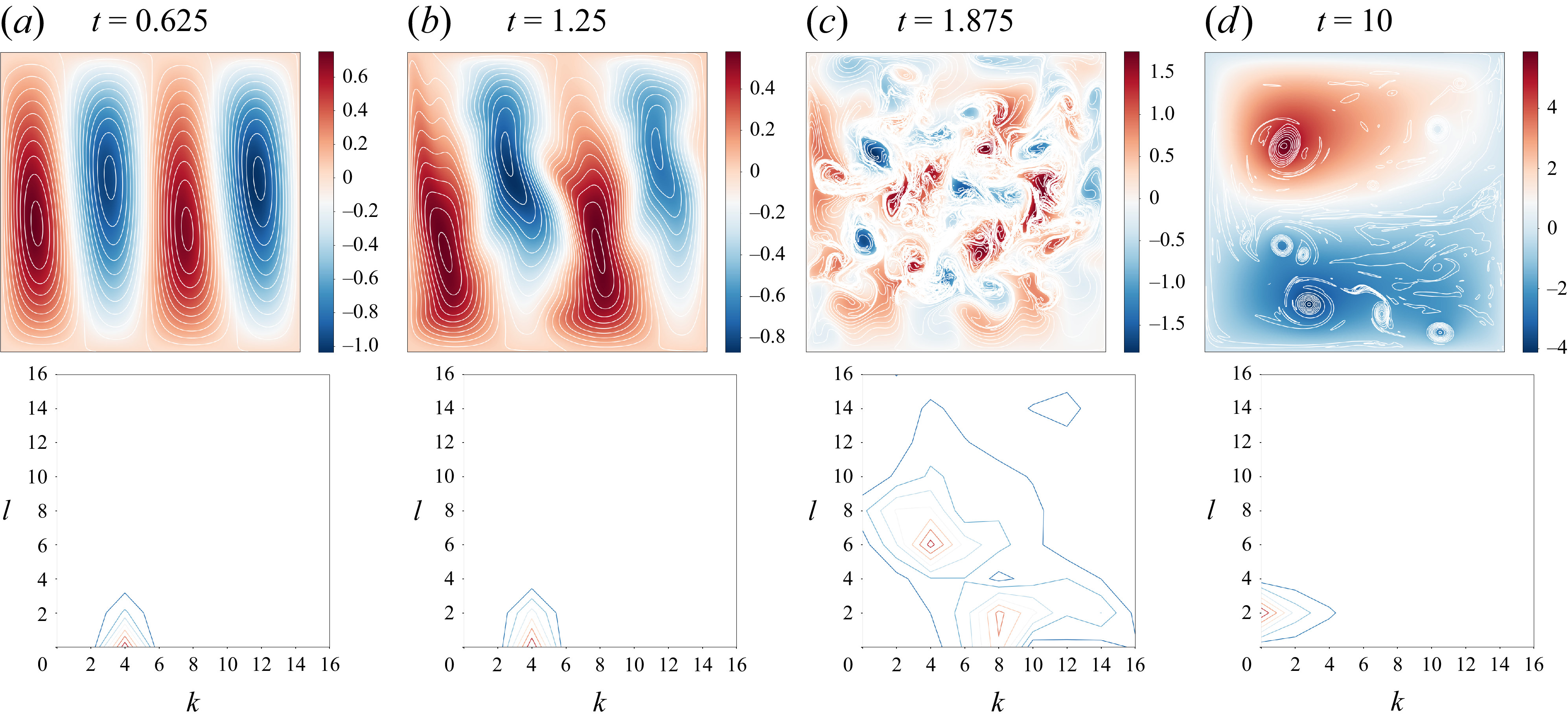


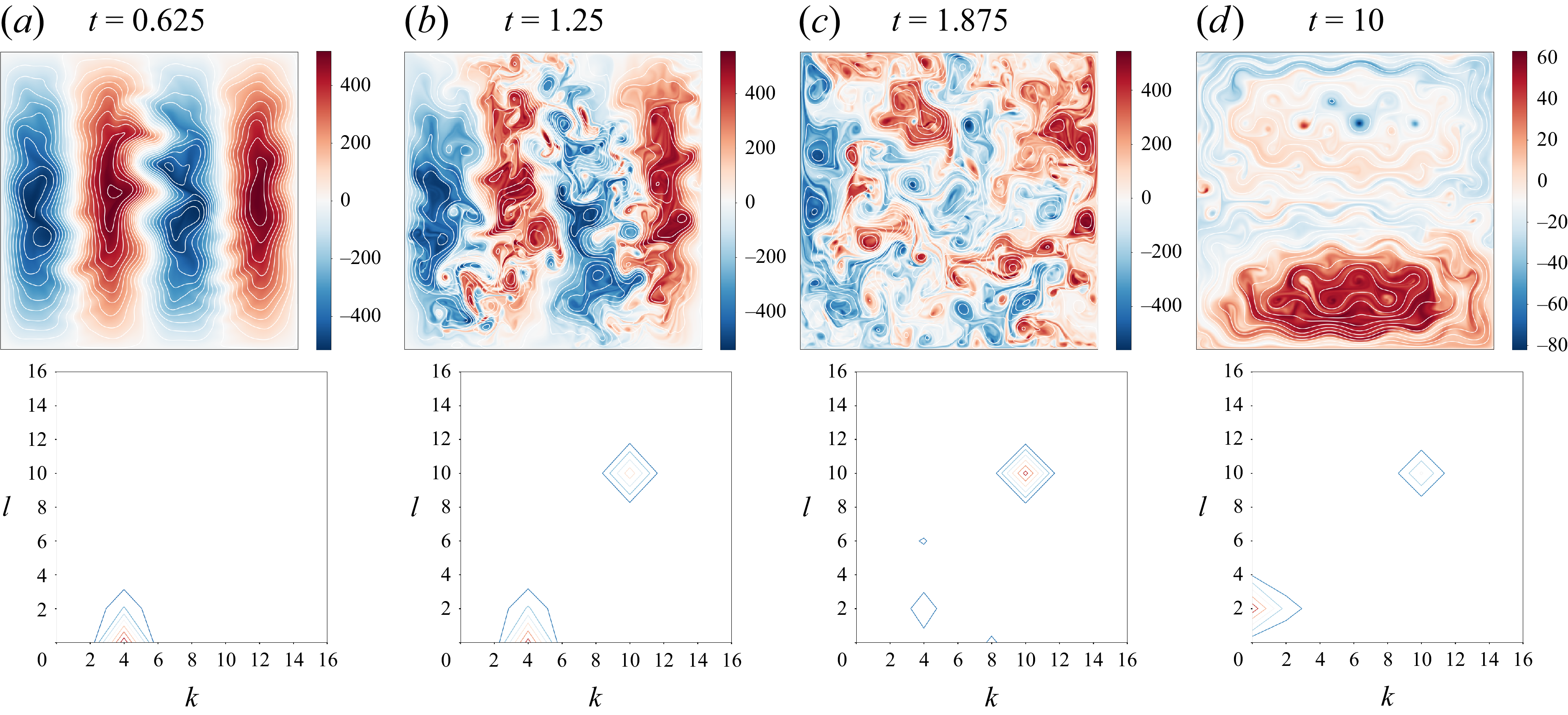

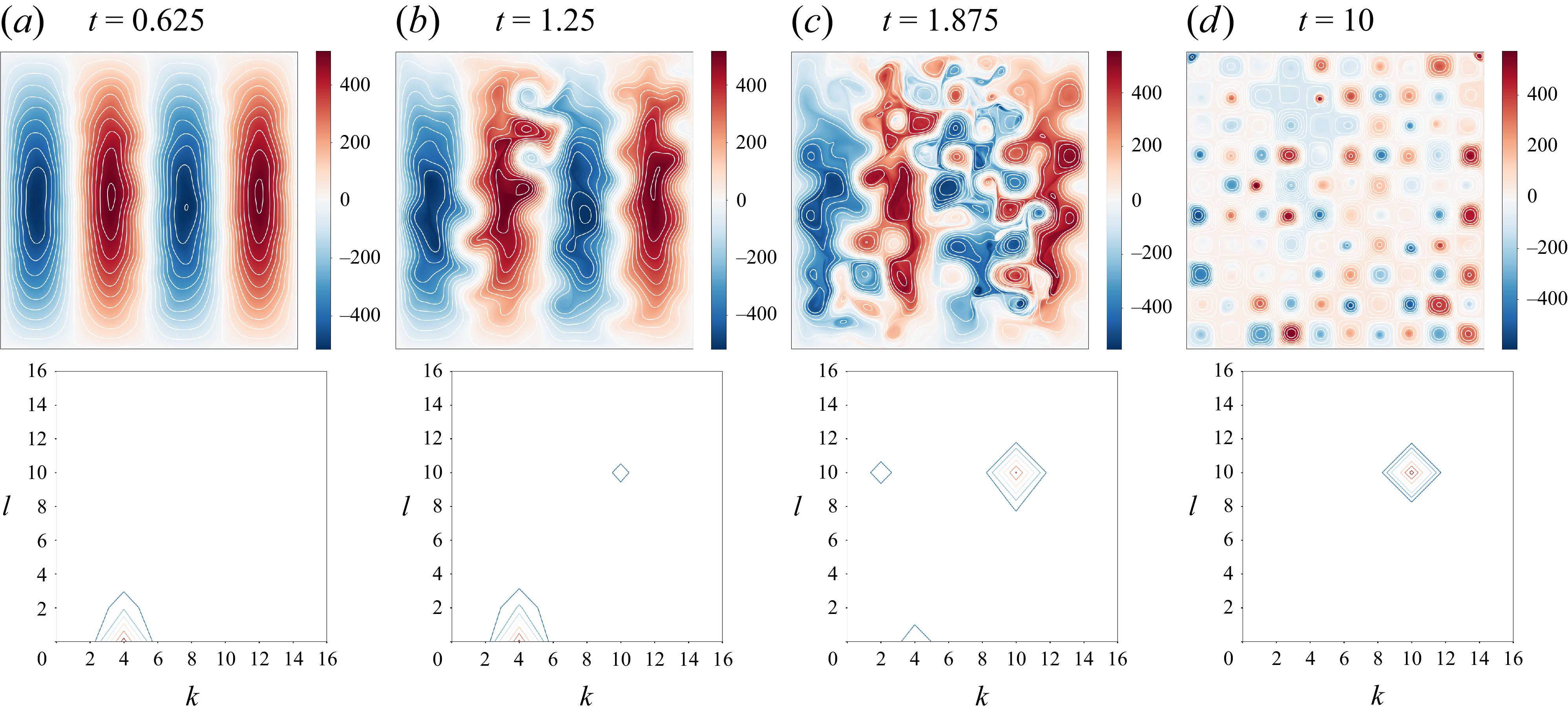

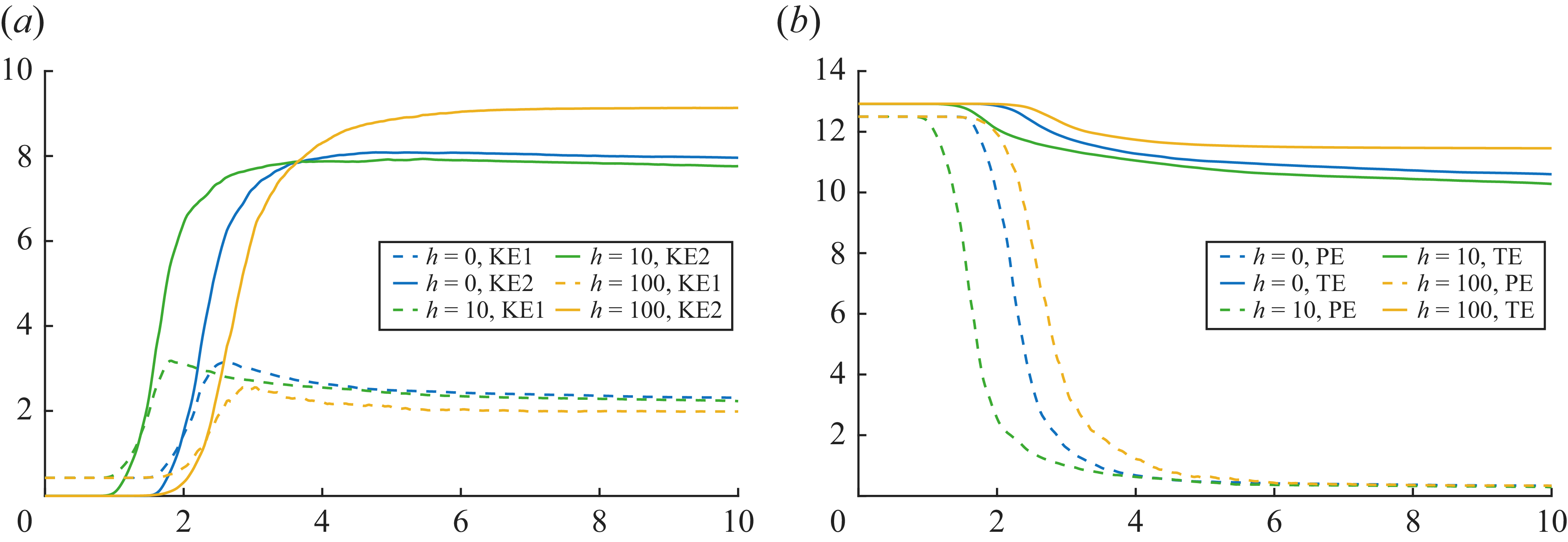

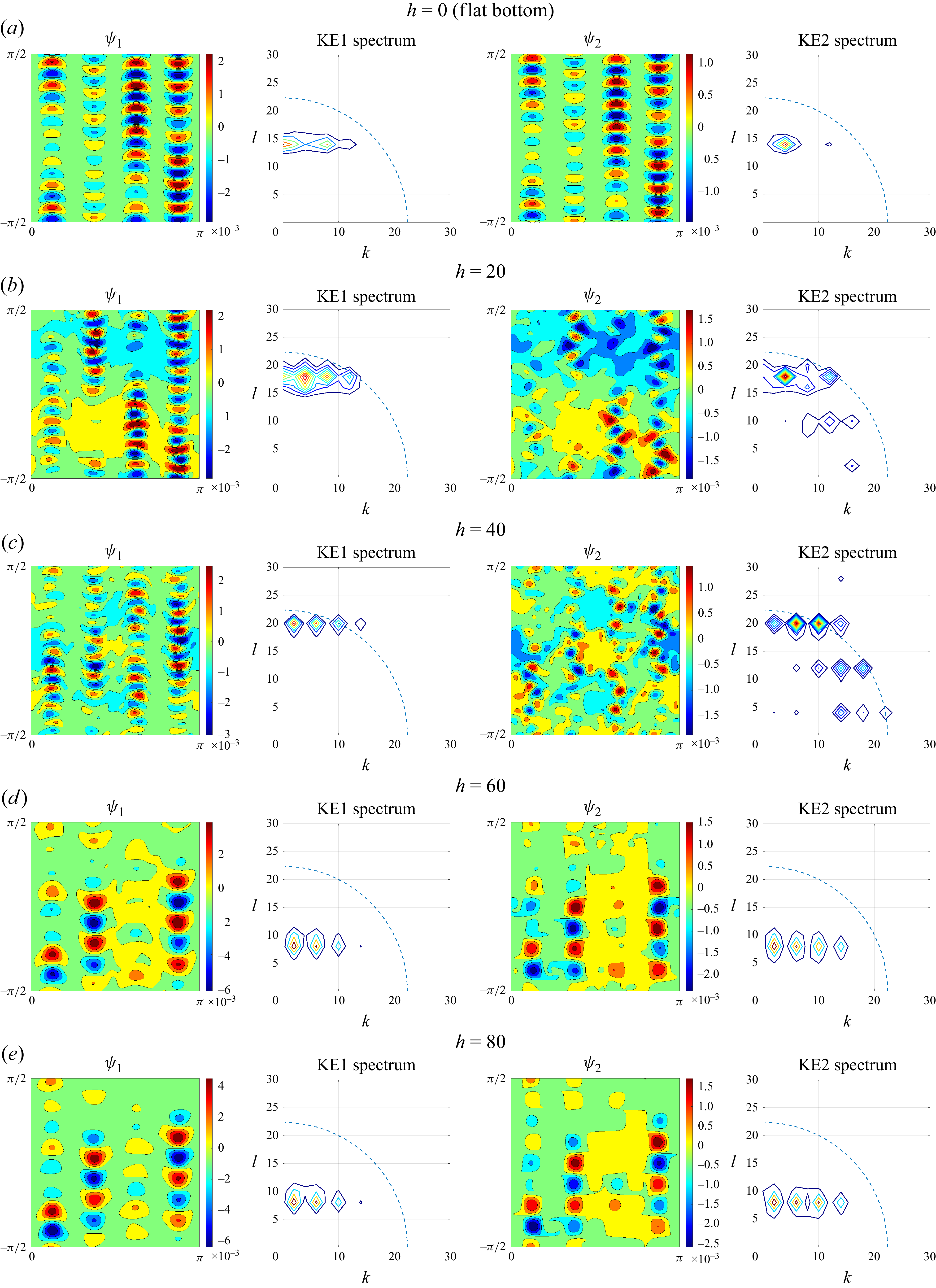


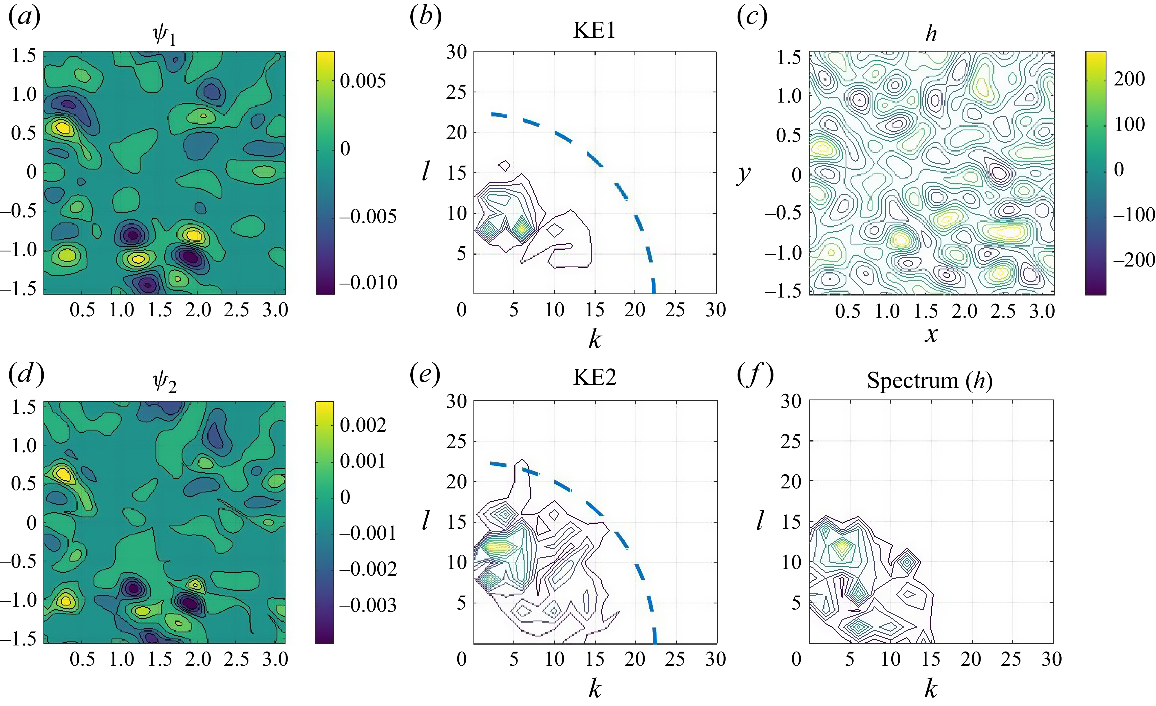

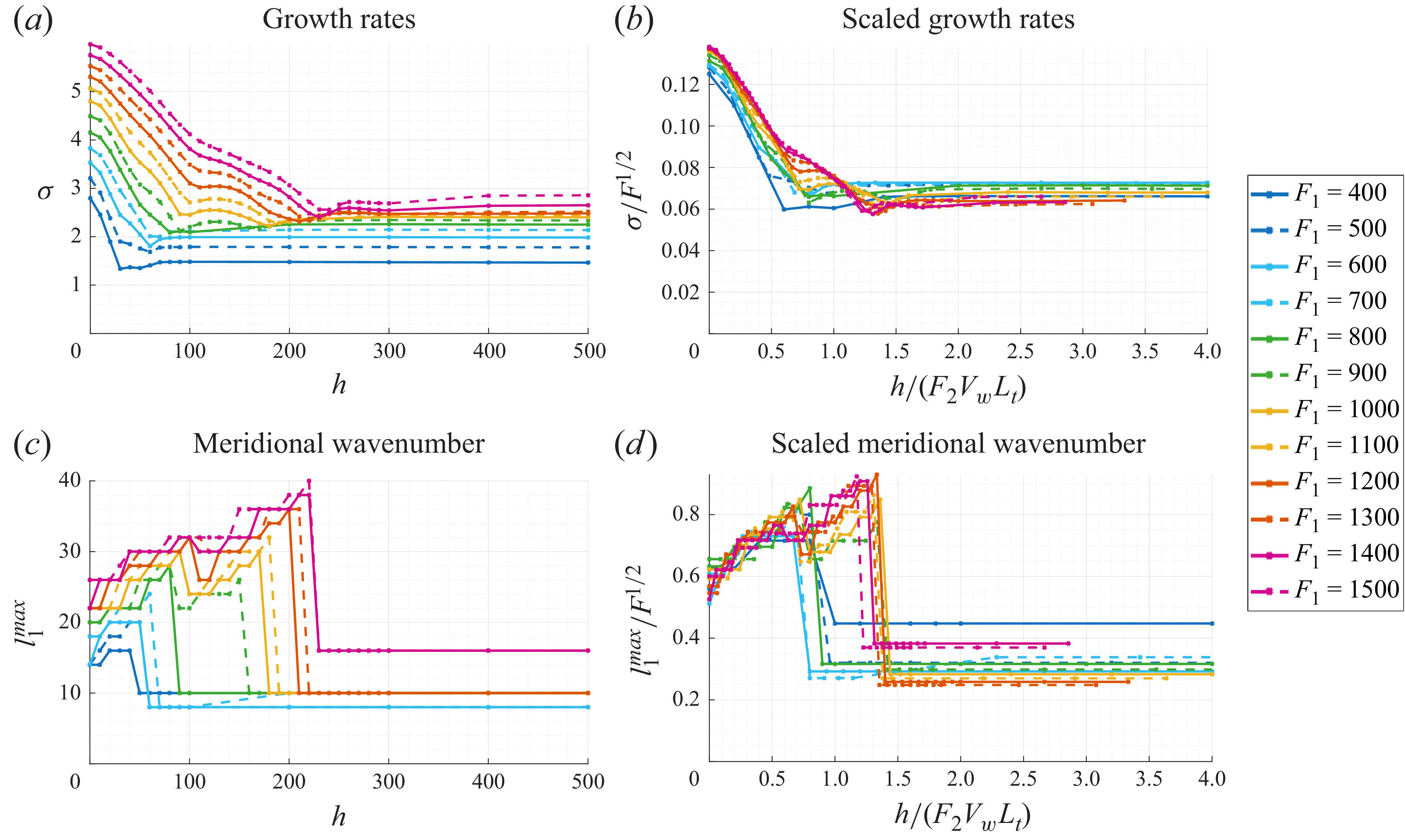
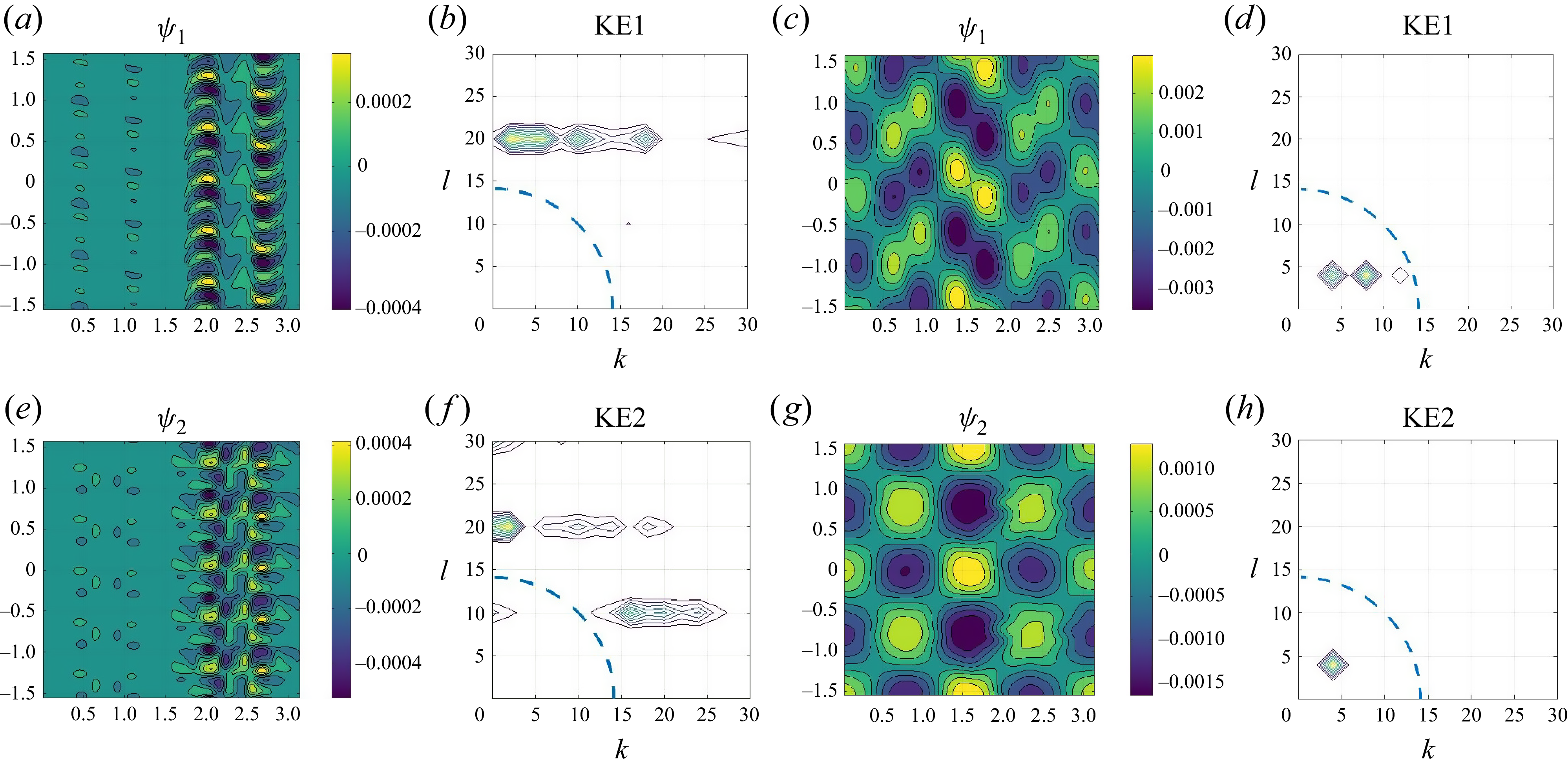


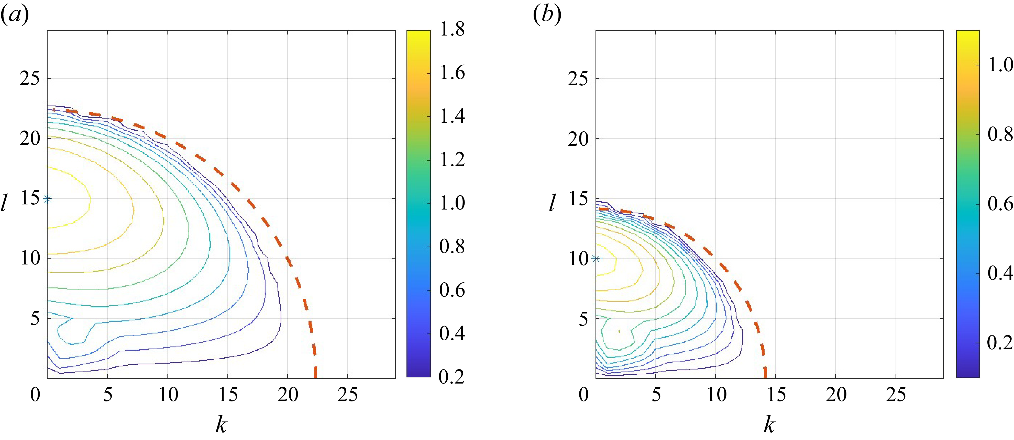


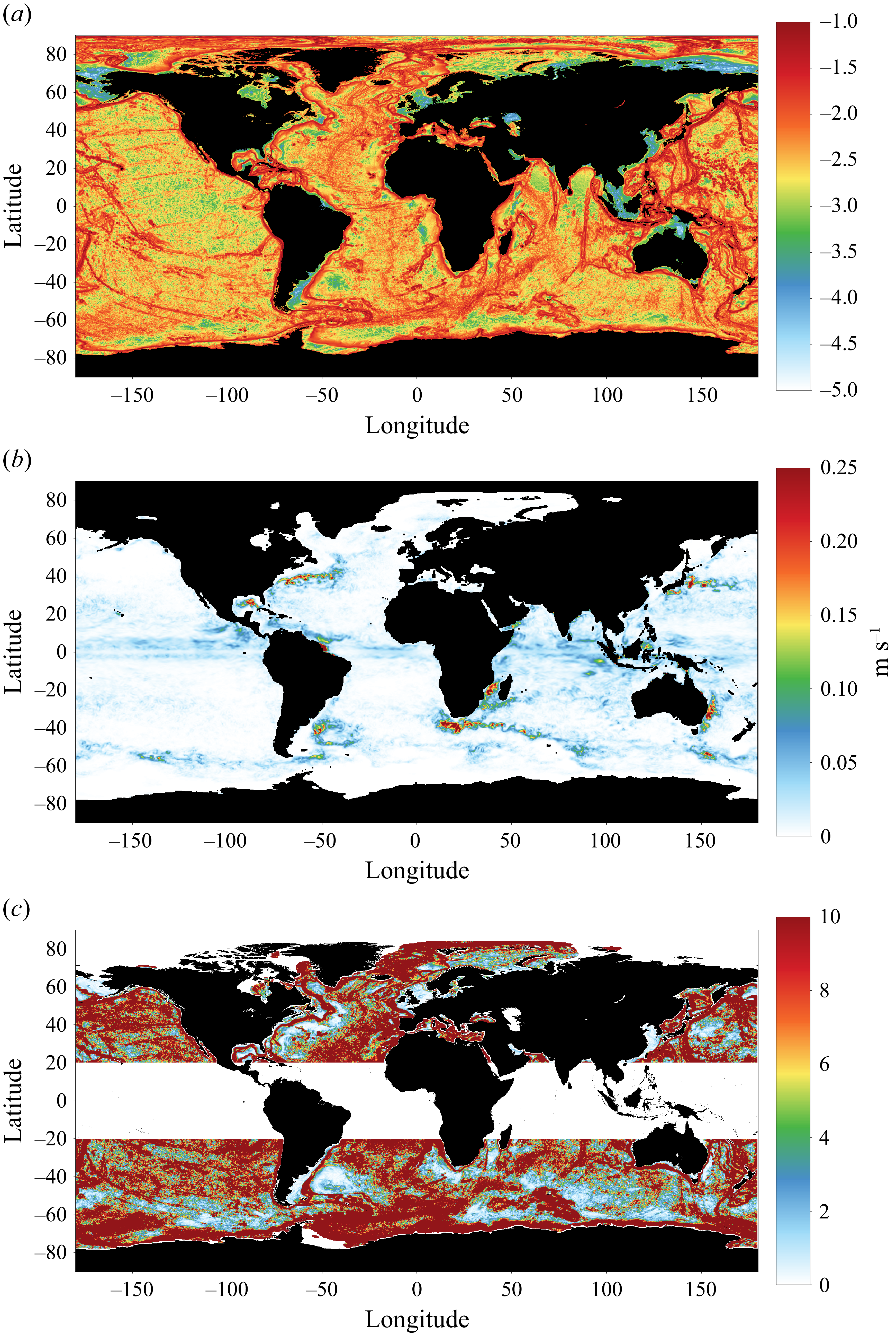


 Open access