


1. Introduction
In both the solar corona and solar wind, observations show that proton heating is typically much greater than the electron heating, with minor ions heated even more strongly, and moreover that ion heating is mainly perpendicular to the magnetic field (Kohl et al. Reference Kohl1998; Marsch et al. Reference Marsch, Goertz and Richter1982, Reference Marsch, Ao and Tu2004; Antonucci, Dodero & Giordano Reference Antonucci, Dodero and Giordano2000; Hellinger et al. Reference Hellinger, Trávníček, Kasper and Lazarus2006; Kasper et al. Reference Kasper, Klein, Weber, Maksimovic, Zaslavsky, Bale, Maruca, Stevens and Case2017; Bowen et al. Reference Bowen2020). Characterising ion heating is therefore essential for the thermodynamics of this system (Parker Reference Parker1965). More generally, correctly parametrising the ratio of ion-to-electron heating in plasma turbulence is of great interest for the interpretation of many remote astrophysical observations (Chael et al. Reference Chael, Rowan, Narayan, Johnson and Sironi2018).
What is the source of free energy for the observed heating? One successful model is heating from the Alfvénic plasma turbulence ubiquitous in the solar wind (Belcher & Davis Reference Belcher and Davis1971; Chen Reference Chen2016; Chen et al. Reference Chen2020) and corona (De Pontieu et al. Reference De Pontieu2007); the fluctuation amplitudes are consistent with the observed plasma heating (Chandran & Hollweg Reference Chandran and Hollweg2009; Cranmer et al. Reference Cranmer, Matthaeus, Breech and Kasper2009), suggesting that the solar wind is accelerated and locally heated by the dissipation of these turbulent fluctuations. It is worth noting that because the turbulence has only a very small compressive component (Klein et al. Reference Klein, Howes, TenBarge, Bale, Chen and Salem2012), the ion heating within the gyrokinetic approximation would be much smaller to explain the observations (Schekochihin et al. Reference Schekochihin, Cowley, Dorland, Hammett, Howes, Quataert and Tatsuno2009, Reference Schekochihin, Kawazura and Barnes2019; Kawazura et al. Reference Kawazura, Schekochihin, Barnes, TenBarge, Tong, Klein and Dorland2020).
Several theoretical models have been proposed to explain ion heating in turbulence. First, cyclotron resonant heating (Hollweg & Isenberg Reference Hollweg and Isenberg2002; Chandran et al. Reference Chandran, Li, Rogers, Quataert and Germaschewski2010; Isenberg & Vasquez Reference Isenberg and Vasquez2011, Reference Isenberg and Vasquez2019; Bowen et al. Reference Bowen2024) occurs when, in the frame moving with an ion’s parallel velocity
 $v_\parallel$
, a wave’s frequency
$v_\parallel$
, a wave’s frequency
 $\omega - k_\parallel v_\parallel$
matches the gyrofrequency
$\omega - k_\parallel v_\parallel$
matches the gyrofrequency
 $\varOmega _i$
: hence, ‘resonant’,
$\varOmega _i$
: hence, ‘resonant’,
 $\omega - k_\parallel v_\parallel - n \varOmega _i =0$
. This is often discussed in the framework of quasilinear theory (Kennel & Engelmann Reference Kennel and Engelmann1966; Stix Reference Stix1992), where the resulting diffusion of energy in phase space is derived assuming a spectrum of infinite plane waves and considering only the resonant response.
$\omega - k_\parallel v_\parallel - n \varOmega _i =0$
. This is often discussed in the framework of quasilinear theory (Kennel & Engelmann Reference Kennel and Engelmann1966; Stix Reference Stix1992), where the resulting diffusion of energy in phase space is derived assuming a spectrum of infinite plane waves and considering only the resonant response.
Another important model, closer in approach to that of the present paper, is stochastic heating (McChesney, Stern & Bellan Reference McChesney, Stern and Bellan1987; Chandran et al. Reference Chandran, Li, Rogers, Quataert and Germaschewski2010), in which ions random-walk in energy due to uncorrelated kicks from ion-scale fluctuations. In the model of Chandran et al. (Reference Chandran, Li, Rogers, Quataert and Germaschewski2010), this results in a heating rate
 $Q_\perp \sim \delta u_\rho ^3/\rho _{\textrm{th}} \exp (-c_2 v_{\textrm{th}}/\delta u_\rho )$
, where
$Q_\perp \sim \delta u_\rho ^3/\rho _{\textrm{th}} \exp (-c_2 v_{\textrm{th}}/\delta u_\rho )$
, where
 $\delta u_\rho$
is the amplitude of
$\delta u_\rho$
is the amplitude of
 $E\times B$
velocity fluctuations at the gyroscale
$E\times B$
velocity fluctuations at the gyroscale
 $\rho _{\textrm{th}}$
, and the exponential suppression factor was added empirically to account for the near-conservation of the magnetic moment at low frequencies and small amplitudes. One advantage of stochastic heating as opposed to cyclotron resonant heating is that it does not require an exact resonance nor does it assume that the fluctuations resemble infinite plane waves. This allows one to easily incorporate the observed intermittent probability distribution of fluctuation amplitudes (Chandran, Schekochihin & Mallet Reference Chandran, Schekochihin and Mallet2015; Mallet & Schekochihin Reference Mallet and Schekochihin2017) at the gyroscale, which can dramatically increase the predicted heating rate (Mallet et al. Reference Mallet, Klein, Chandran, Grošelj, Hoppock, Bowen, Salem and Bale2019; Cerri, Arzamasskiy & Kunz Reference Cerri, Arzamasskiy and Kunz2021).
$\rho _{\textrm{th}}$
, and the exponential suppression factor was added empirically to account for the near-conservation of the magnetic moment at low frequencies and small amplitudes. One advantage of stochastic heating as opposed to cyclotron resonant heating is that it does not require an exact resonance nor does it assume that the fluctuations resemble infinite plane waves. This allows one to easily incorporate the observed intermittent probability distribution of fluctuation amplitudes (Chandran, Schekochihin & Mallet Reference Chandran, Schekochihin and Mallet2015; Mallet & Schekochihin Reference Mallet and Schekochihin2017) at the gyroscale, which can dramatically increase the predicted heating rate (Mallet et al. Reference Mallet, Klein, Chandran, Grošelj, Hoppock, Bowen, Salem and Bale2019; Cerri, Arzamasskiy & Kunz Reference Cerri, Arzamasskiy and Kunz2021).
Observations (Chen et al. Reference Chen, Mallet, Yousef, Schekochihin and Horbury2011) show that the solar wind turbulence is highly anisotropic: fluctuations have very different characteristic length scales parallel (
 $l_\parallel$
) and perpendicular (
$l_\parallel$
) and perpendicular (
 $\lambda$
) to the background magnetic field,
$\lambda$
) to the background magnetic field,
 $l_\parallel \gg l_\perp$
. Modern turbulence theories (Goldreich & Sridhar Reference Goldreich and Sridhar1995; Boldyrev Reference Boldyrev2006) explain this in terms of a critical balance between characteristic time scales associated with linear propagation (
$l_\parallel \gg l_\perp$
. Modern turbulence theories (Goldreich & Sridhar Reference Goldreich and Sridhar1995; Boldyrev Reference Boldyrev2006) explain this in terms of a critical balance between characteristic time scales associated with linear propagation (
 $\tau _{lin}\sim l_\parallel / v_{\rm {A}}$
, with
$\tau _{lin}\sim l_\parallel / v_{\rm {A}}$
, with
 $v_{\textrm{A}}=B_0/\sqrt {4\pi n_p m_p}$
the Alfvén velocity based on the mean magnetic field
$v_{\textrm{A}}=B_0/\sqrt {4\pi n_p m_p}$
the Alfvén velocity based on the mean magnetic field
 $B_0$
) and nonlinear interactions (
$B_0$
) and nonlinear interactions (
 $\tau _{nl}\sim \lambda / \delta u_\lambda$
): the cascade time
$\tau _{nl}\sim \lambda / \delta u_\lambda$
): the cascade time
 $\tau \sim \tau _{lin}\sim \tau _{nl}$
, whence
$\tau \sim \tau _{lin}\sim \tau _{nl}$
, whence
 $l_\parallel / \lambda \sim v_{\textrm{A}}/\delta u_\lambda \gg 1$
. Since the fluctuating field amplitude
$l_\parallel / \lambda \sim v_{\textrm{A}}/\delta u_\lambda \gg 1$
. Since the fluctuating field amplitude
 $\delta u_\lambda$
at scale
$\delta u_\lambda$
at scale
 $\lambda$
is an increasing function of
$\lambda$
is an increasing function of
 $\lambda$
, at progressively smaller scales, the anisotropy
$\lambda$
, at progressively smaller scales, the anisotropy
 $l_\parallel /\lambda$
increases. This means that the fluctuations remain relatively low frequency, with
$l_\parallel /\lambda$
increases. This means that the fluctuations remain relatively low frequency, with
 $\omega \sim 1/\tau \ll \varOmega _i$
, where
$\omega \sim 1/\tau \ll \varOmega _i$
, where
 $\varOmega _i=Z_i e B/m_i c$
is the ion gyrofrequency. This poses a challenge: the magnetic moment
$\varOmega _i=Z_i e B/m_i c$
is the ion gyrofrequency. This poses a challenge: the magnetic moment
 $\mu = m_i v_\perp ^2/B$
is conserved to all orders in
$\mu = m_i v_\perp ^2/B$
is conserved to all orders in
 $\eta \sim \omega /\varOmega _i\ll 1$
(Kruskal Reference Kruskal1962), and so the usual perturbation theory would suggest that perpendicular ion heating should be irrelevant for such anisotropic, small-amplitude turbulence, in contrast to the observations. It is worth noting that ‘to all orders’ is not the same as ‘exactly’: as an example (that will be important in this paper),
$\eta \sim \omega /\varOmega _i\ll 1$
(Kruskal Reference Kruskal1962), and so the usual perturbation theory would suggest that perpendicular ion heating should be irrelevant for such anisotropic, small-amplitude turbulence, in contrast to the observations. It is worth noting that ‘to all orders’ is not the same as ‘exactly’: as an example (that will be important in this paper),
 $\exp (-1/\eta )\neq 0$
, but is ‘zero to all orders’ if
$\exp (-1/\eta )\neq 0$
, but is ‘zero to all orders’ if
 $\eta \ll 1$
, since all derivatives vanish as
$\eta \ll 1$
, since all derivatives vanish as
 $\eta \to 0$
.
$\eta \to 0$
.
In addition to turbulence, magnetic reconnection has been proposed as a mechanism for coronal heating (Klimchuk Reference Klimchuk2015) and also as a heating mechanism within the turbulence itself (Shay et al. Reference Shay, Haggerty, Matthaeus, Parashar, Wan and Wu2018). In fact, turbulent heating and reconnection heating may not be as distinct as traditionally thought. The turbulent cascade naturally leads to the formation of extended current sheets (Boldyrev Reference Boldyrev2006; Chandran et al. Reference Chandran, Schekochihin and Mallet2015; Mallet & Schekochihin Reference Mallet and Schekochihin2017), which reconnect once their width becomes sufficiently small (Boldyrev & Loureiro Reference Boldyrev and Loureiro2017; Cerri & Califano Reference Cerri and Califano2017; Comisso et al. Reference Comisso, Lingam, Huang and Bhattacharjee2017; Franci et al. Reference Franci, Cerri, Califano, Landi, Papini, Verdini, Matteini, Jenko and Hellinger2017; Loureiro & Boldyrev Reference Loureiro and Boldyrev2017a ; Mallet, Schekochihin & Chandran Reference Mallet, Schekochihin and Chandran2017; Vech et al. Reference Vech, Mallet, Klein and Kasper2018; Dong et al. Reference Dong, Wang, Huang, Comisso, Sandstrom and Bhattacharjee2022). Similarly, approaching the problem from the ‘reconnection end’, extended reconnecting current sheets are often violently unstable, leading naturally to strong turbulence (Loureiro, Schekochihin & Cowley Reference Loureiro, Schekochihin and Cowley2007; Bhattacharjee et al. Reference Bhattacharjee, Huang, Yang and Rogers2009; Huang & Bhattacharjee Reference Huang and Bhattacharjee2016). Seeking to explain preferential heavy-ion heating in the corona and solar flares, Drake et al. (Reference Drake, Swisdak, Phan, Cassak, Shay, Lepri, Lin, Quataert and Zurbuchen2009a ) developed a theory of perpendicular ion heating in reconnection exhausts, supported by numerical simulations. Drake et al. (Reference Drake, Cassak, Shay, Swisdak and Quataert2009b ) showed that in guide-field reconnection, strong ion heating only occurs if the characteristic time scale to transit the exhaust is shorter than the ion’s gyroperiod. This behaviour has similarities to the stochastic heating in turbulence.
All three of cyclotron-resonant, stochastic and reconnection perpendicular ion heating share a common feature: they require the conservation of the magnetic moment to be broken. In the case of stochastic and reconnection heating, this leads to a ‘threshold’ which must be satisfied for strong ion heating to be possible. Likewise, in cyclotron resonant heating, the resonance condition must be satisfied (we will argue that this ‘sharper’ behaviour is a consequence of the plane-wave assumption). Johnston, Squire & Meyrand (Reference Johnston, Squire and Meyrand2025) noticed the similarities between cyclotron-resonant and stochastic heating, and found that the heating in their test-particle simulations was well described by a single exponential suppression factor modelling both cyclotron-resonant heating in imbalanced turbulence and stochastic heating in balanced turbulence. In related work in a different physical setting, namely electron scattering in the radiation belts, a similarly close relationship between electron scattering by strongly nonlinear coherent structures (electron holes) and quasilinear theory was also previously discussed by Vasko et al. (Reference Vasko, Agapitov, Mozer, Artemyev, Krasnoselskikh and Bonnell2017; Reference Vasko, Krasnoselskikh, Mozer and Artemyev2018).
In this paper, we develop a new framework that describes perpendicular ion heating. We analytically study the response of an ion to a localised, coherent fluctuation in the electromagnetic fields, with the fluctuating electric
 $\delta \boldsymbol{E}$
and magnetic
$\delta \boldsymbol{E}$
and magnetic
 $\delta {\boldsymbol{B}}$
fields tending to zero at
$\delta {\boldsymbol{B}}$
fields tending to zero at
 $t=\pm \infty$
, an approach to our knowledge first taken by Krall & Rosenbluth (Reference Krall and Rosenbluth1964) for electric field fluctuations and for general adiabatic invariants by Landau & Lifshitz (Reference Landau and Lifshitz1976). Quite generically, we find that the perpendicular ion kinetic energy
$t=\pm \infty$
, an approach to our knowledge first taken by Krall & Rosenbluth (Reference Krall and Rosenbluth1964) for electric field fluctuations and for general adiabatic invariants by Landau & Lifshitz (Reference Landau and Lifshitz1976). Quite generically, we find that the perpendicular ion kinetic energy
 $m_i v_\perp ^2/2$
changes by an amount of order
$m_i v_\perp ^2/2$
changes by an amount of order
 \begin{equation} m_i \varDelta \sim m_i\epsilon \exp (-1/\eta ), \end{equation}
where
 $\varDelta$
is the change in
$\varDelta$
is the change in
 $v_\perp ^2$
,
$v_\perp ^2$
,
 $\epsilon \sim \delta B/B_0 \sim c\delta E/B_0v_\perp$
is the normalised amplitude of the fluctuations and
$\epsilon \sim \delta B/B_0 \sim c\delta E/B_0v_\perp$
is the normalised amplitude of the fluctuations and
 $\eta \sim 1/\tau \varOmega _i$
, where
$\eta \sim 1/\tau \varOmega _i$
, where
 $\tau$
is a characteristic time scale over which
$\tau$
is a characteristic time scale over which
 $\delta {\boldsymbol{B}}$
and
$\delta {\boldsymbol{B}}$
and
 $\delta \boldsymbol{E}$
vary. The threshold for strong ion heating to occur is encoded in the exponential factor:
$\delta \boldsymbol{E}$
vary. The threshold for strong ion heating to occur is encoded in the exponential factor:
 $\mu$
-conservation is lost when
$\mu$
-conservation is lost when
 $\eta \sim 1$
and the fluctuations vary significantly over one gyroperiod. For
$\eta \sim 1$
and the fluctuations vary significantly over one gyroperiod. For
 $\eta \ll 1$
, the magnetic moment is conserved to all orders, but not exactly: for many systems, this is enough to provide significant heating over long time scales. After setting up the system of equations (§ 2), in § 3, we proceed to expand the amplitude of the fluctuating fields, deriving analytic expressions for the change in perpendicular and parallel energy as well as how this depends on the length scale of the fluctuations. We also derive general formulae for the diffusion coefficient and heating rate, and outline how our theory should be applied to different physical systems. We then explicitly show how our results apply to both Alfvénic turbulence (§ 4) and to reconnection (§ 5). Finally, we discuss the relationship of our model to earlier theories, and what the implications of our results are for astrophysical and space plasma turbulence and reconnection heating.
$\eta \ll 1$
, the magnetic moment is conserved to all orders, but not exactly: for many systems, this is enough to provide significant heating over long time scales. After setting up the system of equations (§ 2), in § 3, we proceed to expand the amplitude of the fluctuating fields, deriving analytic expressions for the change in perpendicular and parallel energy as well as how this depends on the length scale of the fluctuations. We also derive general formulae for the diffusion coefficient and heating rate, and outline how our theory should be applied to different physical systems. We then explicitly show how our results apply to both Alfvénic turbulence (§ 4) and to reconnection (§ 5). Finally, we discuss the relationship of our model to earlier theories, and what the implications of our results are for astrophysical and space plasma turbulence and reconnection heating.
2. Normalised equations
The equations of motion for an ion of charge
 $Z_i e$
and mass
$Z_i e$
and mass
 $m_i$
in a general electromagnetic field are
$m_i$
in a general electromagnetic field are
 \begin{equation} \frac {{\rm d}^2 \boldsymbol{R}}{\mathrm{d}t^2} = \frac {Z_ie}{m_i}\left [\boldsymbol{E} + \frac {\mathrm{d}{\boldsymbol{R}}/\mathrm{d} t\times {\boldsymbol{B}}}{c}\right ]\!. \end{equation}
For the magnetic and electric field, we take
 \begin{equation} {\boldsymbol{B}} = B_0\left [\hat {\boldsymbol{z}} + \varepsilon b(y,z,\varOmega _i t)\hat {\boldsymbol{x}}\right]\!, \quad \boldsymbol{E} = \frac {\varepsilon v_{\perp 0} B_0}{c}g(y,z,\varOmega _it)\hat {\boldsymbol{y}}, \end{equation}
where we assume
 $\varepsilon \ll 1$
, and
$\varepsilon \ll 1$
, and
 $v_{\perp 0}$
is the perpendicular ion velocity at
$v_{\perp 0}$
is the perpendicular ion velocity at
 $t=-\infty$
. Our neglect of
$t=-\infty$
. Our neglect of
 $B_y$
and
$B_y$
and
 $E_x$
will not change the physical conclusions of our calculation (while making it somewhat less cumbersome), but ignoring
$E_x$
will not change the physical conclusions of our calculation (while making it somewhat less cumbersome), but ignoring
 $E_z$
and fluctuations in
$E_z$
and fluctuations in
 $B_z$
removes the possibility of Landau and transit-time energisation of the particle: we wish to focus solely on the cyclotron interaction. If this makes one uncomfortable, it may be justified by considering low ion beta
$B_z$
removes the possibility of Landau and transit-time energisation of the particle: we wish to focus solely on the cyclotron interaction. If this makes one uncomfortable, it may be justified by considering low ion beta
 $\beta _i = 8\pi n_i T_i/B_0^2$
, where such effects (for the ions) are typically relatively weak since the typical phase velocity
$\beta _i = 8\pi n_i T_i/B_0^2$
, where such effects (for the ions) are typically relatively weak since the typical phase velocity
 $v_{\textrm{ph}}\sim v_{\textrm{A}} \gg v_{\textrm{th}}$
. Note we have also assumed that the electric and magnetic fields do not vary in the
$v_{\textrm{ph}}\sim v_{\textrm{A}} \gg v_{\textrm{th}}$
. Note we have also assumed that the electric and magnetic fields do not vary in the
 $\hat {\boldsymbol{x}}$
direction. We assume that the functions
$\hat {\boldsymbol{x}}$
direction. We assume that the functions
 $b$
and
$b$
and
 $g$
are analytic for
$g$
are analytic for
 $t$
real and that
$t$
real and that
 $b(y,z,\pm \infty )=g(y,z,\pm \infty )=0$
. Here,
$b(y,z,\pm \infty )=g(y,z,\pm \infty )=0$
. Here,
 $b$
and
$b$
and
 $g$
are related according to Faraday’s law,
$g$
are related according to Faraday’s law,
 \begin{equation} \partial _t b = v_{\perp 0} \partial _z g. \end{equation}
We carry out our calculation in the frame moving at
 $v_{\parallel 0}$
, the parallel velocity of the ion at
$v_{\parallel 0}$
, the parallel velocity of the ion at
 $t=-\infty$
, and normalise according to
$t=-\infty$
, and normalise according to
 \begin{equation} X= x/\rho , \quad Y= y/\rho , \quad Z=(z-v_{\parallel 0} t)/\rho \quad T = \varOmega _{i} t, \end{equation}
where
 $\varOmega _i=Z_i eB/m_ic$
is the ion gyrofrequency and
$\varOmega _i=Z_i eB/m_ic$
is the ion gyrofrequency and
 $\rho = v_{\perp 0}/\varOmega _i$
is the ion gyroradius. Later, it will be useful to write
$\rho = v_{\perp 0}/\varOmega _i$
is the ion gyroradius. Later, it will be useful to write
 $g$
and
$g$
and
 $b$
in terms of their Fourier transforms in
$b$
in terms of their Fourier transforms in
 $Y$
,
$Y$
,
 \begin{align} g(Y,Z,T) &= \frac {1}{2\pi }\int _{-\infty }^\infty \tilde {g}(K,Z,\eta _KT)e^{iKY}\mathrm{d} K,\nonumber \\ b(Y,Z,T) &= \frac {1}{2\pi }\int _{-\infty }^\infty \tilde {b}(K,Z,\eta _KT)e^{iKY}\mathrm{d} K. \end{align}
The dimensionless quantity
 $\eta _K$
appearing in the arguments of
$\eta _K$
appearing in the arguments of
 $\tilde {g}$
and
$\tilde {g}$
and
 $\tilde {b}$
is a bookkeeping parameter that describes how fast the fields at wavenumber
$\tilde {b}$
is a bookkeeping parameter that describes how fast the fields at wavenumber
 $K$
vary relative to the cyclotron motion of the particle: for
$K$
vary relative to the cyclotron motion of the particle: for
 $\eta _K\sim 1$
, the fields can vary significantly over one orbit, while for
$\eta _K\sim 1$
, the fields can vary significantly over one orbit, while for
 $\eta _K\ll 1$
, they only vary a small amount. Importantly, we do not require
$\eta _K\ll 1$
, they only vary a small amount. Importantly, we do not require
 $\eta _K\ll 1$
: in fact, for the main calculation that appears in § 3, we formally require
$\eta _K\ll 1$
: in fact, for the main calculation that appears in § 3, we formally require
 $\varepsilon \ll \eta _K$
for all
$\varepsilon \ll \eta _K$
for all
 $K\gtrsim 1$
, i.e.
$K\gtrsim 1$
, i.e.
 $\eta _K$
cannot be too small. The case with
$\eta _K$
cannot be too small. The case with
 $\eta _K\sim \varepsilon$
or smaller is dealt with in Appendix C, where we show that our results can be extended to this case with no changes. If
$\eta _K\sim \varepsilon$
or smaller is dealt with in Appendix C, where we show that our results can be extended to this case with no changes. If
 $\eta _K$
in some system happens to be constant with
$\eta _K$
in some system happens to be constant with
 $K$
, we will sometimes simply write
$K$
, we will sometimes simply write
 $\eta$
. Denoting
$\eta$
. Denoting
 $\mathrm{d}f/\mathrm{d} T=\dot {f}$
, the equations are then
$\mathrm{d}f/\mathrm{d} T=\dot {f}$
, the equations are then
 \begin{align} \ddot {X} &= \dot {Y}, \end{align}
 \begin{align} \ddot {Y} &= -\dot {X} + \varepsilon g(Y,Z,T), \end{align}
 \begin{align} \ddot {Z} &= -\varepsilon \dot {Y} b(Y,Z,T),\\[6pt] \nonumber \end{align}
which we will solve subject to the arbitrary choices for the phase of the particle
 $X(0)=1$
,
$X(0)=1$
,
 $\dot {X}(0)=0$
,
$\dot {X}(0)=0$
,
 $Y(0)=0$
,
$Y(0)=0$
,
 $\dot {Y}(0)=1$
,
$\dot {Y}(0)=1$
,
 $Z(0)=0$
, and we have chosen the inertial frame of reference such that
$Z(0)=0$
, and we have chosen the inertial frame of reference such that
 $\dot {Z}(-\infty )=0$
. In the normalised variables, Faraday’s law is
$\dot {Z}(-\infty )=0$
. In the normalised variables, Faraday’s law is
 \begin{equation} \partial _T b = \partial _Z g. \end{equation}
Integrating (2.6), taking the constant of integration to be zero and inserting the resulting equation into (2.7), we have
 \begin{align} \dot {X} &= Y, \end{align}
 \begin{align} \ddot {Y}+Y &= \varepsilon g(Y,Z,T).\\[6pt] \nonumber \end{align}
3. Solution for
 $\varepsilon \ll \eta _K\sim 1$

We expand
 \begin{align} X= X_0 + \varepsilon X_1 + \varepsilon ^2 X_2 +\ldots \quad\!\! Y= Y_0 + \varepsilon Y_1 + \varepsilon ^2 Y_2 +\ldots \quad\!\!\! Z= Z_0 + \varepsilon Z_1 + \varepsilon ^2 Z_2 +\ldots \end{align}
and proceed with our calculation.Footnote
1
At zeroth order in
 $\varepsilon$
, we just have the gyration of the particle about the background field,
$\varepsilon$
, we just have the gyration of the particle about the background field,
 \begin{equation} X_0=-\cos {T}, \quad Y_0= \sin {T}, \quad Z_0=0, \end{equation}
according to the (arbitrary) conditions we set for
 $T=0$
. At first order in
$T=0$
. At first order in
 $\varepsilon$
, inserting the zeroth-order solution above for
$\varepsilon$
, inserting the zeroth-order solution above for
 $Z_0$
and
$Z_0$
and
 $\dot {Y}_0$
into (2.11) and (2.8),
$\dot {Y}_0$
into (2.11) and (2.8),
 \begin{align} \ddot {Y}_1 + Y_1 &= g(\sin T,0,T), \end{align}
 \begin{align} \ddot {Z}_1 &= - b(\sin T,0,T)\cos (T).\\[6pt] \nonumber \end{align}
Equation (3.3) may be solved by Fourier transforming in time and back again; the solution is
 \begin{equation} Y_1 = \int _{-\infty }^T \sin (T-T') g(\sin T',0,T')\mathrm{d} T' = \dot {X}_1, \end{equation}
and the first-order
 $Y$
-velocity is
$Y$
-velocity is
 \begin{equation} \dot {Y}_1 = \int _{-\infty }^T \cos (T-T')g(\sin T',0,T')\mathrm{d} T'. \end{equation}
To make further progress, we Fourier transform in
 $Y$
according to (2.5), and use the identity
$Y$
according to (2.5), and use the identity
 \begin{equation} e^{iK\sin T} = \sum _{n=-\infty }^\infty J_n(K) e^{inT}, \end{equation}
where
 $J_n$
are Bessel functions of the first kind. This results in
$J_n$
are Bessel functions of the first kind. This results in
 \begin{align} \dot {Y}_1 &= \int _{-\infty }^T \cos (T-T')\frac {1}{2\pi }\int _{-\infty }^\infty \tilde {g}(K,0,\eta _KT')\sum _{n=-\infty }^\infty J_n(K)e^{inT'}\,\mathrm{d} K\,\mathrm{d} T',\nonumber \\ &= \cos T \int _{-\infty }^T \cos T'\frac {1}{2\pi }\int _{-\infty }^\infty \tilde {g}(K,0,\eta _KT')\sum _{n=-\infty }^\infty J_n(K)e^{inT'}\,\mathrm{d} K\,\mathrm{d} T'\nonumber \\ &\quad +\sin T \int _{-\infty }^T \sin T'\frac {1}{2\pi }\int _{-\infty }^\infty \tilde {g}(K,0,\eta _KT')\sum _{n=-\infty }^\infty J_n(K)e^{inT'}\,\mathrm{d} K\,\mathrm{d} T'. \end{align}
Similarly, we have
 \begin{align} \dot {X}_1 &= \int _{-\infty }^T \sin (T-T')\frac {1}{2\pi }\int _{-\infty }^\infty \tilde {g}(K,0,\eta _KT')\sum _{n=-\infty }^\infty J_n(K)e^{inT'}\,\mathrm{d} K\,\mathrm{d} T',\nonumber \\ &= \sin T \int _{-\infty }^T \cos T'\frac {1}{2\pi }\int _{-\infty }^\infty \tilde {g}(K,0,\eta _KT')\sum _{n=-\infty }^\infty J_n(K)e^{inT'}\,\mathrm{d} K\,\mathrm{d} T'\nonumber \\ &\quad -\cos T \int _{-\infty }^T \sin T'\frac {1}{2\pi }\int _{-\infty }^\infty \tilde {g}(K,0,\eta _KT')\sum _{n=-\infty }^\infty J_n(K)e^{inT'}\,\mathrm{d} K\,\mathrm{d} T'. \end{align}
Combining the sinusoids and
 $e^{inT'}$
factors in the integrands, and using the identity
$e^{inT'}$
factors in the integrands, and using the identity
 $J_{n-1}(K)+J_{n+1}(K) = 2 nJ_n(K)/K$
,
$J_{n-1}(K)+J_{n+1}(K) = 2 nJ_n(K)/K$
,
 \begin{align} \dot {Y}_1 &= \frac {1}{2\pi }\cos T \int _{-\infty }^T\int _{-\infty }^\infty \tilde {g}(K,0,\eta _KT')\sum _{n=-\infty }^\infty \frac {nJ_n(K)}{K}e^{inT'}\,\mathrm{d} K\,\mathrm{d} T'\nonumber \\ &\quad \,+\frac {1}{2\pi }\sin T \int _{-\infty }^T \int _{-\infty }^\infty \tilde {g}(K,0,\eta _KT')\sum _{n=-\infty }^\infty \frac {J_{n-1}(K)-J_{n+1}(K)}{2i}e^{inT'}\,\mathrm{d} K\,\mathrm{d} T'. \end{align}
Likewise, one finds
 \begin{align} \dot {X}_1 &= \frac {1}{2\pi }\sin T \int _{-\infty }^T\int _{-\infty }^\infty \tilde {g}(K,0,\eta _KT')\sum _{n=-\infty }^\infty \frac {nJ_n(K)}{K}e^{inT'}\,\mathrm{d} K\,\mathrm{d} T'\nonumber \\ &\quad \,-\frac {1}{2\pi }\cos T \int _{-\infty }^T \int _{-\infty }^\infty \tilde {g}(K,0,\eta _KT')\sum _{n=-\infty }^\infty \frac {J_{n-1}(K)-J_{n+1}(K)}{2i}e^{inT'}\,\mathrm{d} K\,\mathrm{d} T'. \end{align}
Finally, using (2.5) to Fourier transform
 $b(Y,Z,T)$
, the first-order parallel velocity is given by
$b(Y,Z,T)$
, the first-order parallel velocity is given by
 \begin{equation} \dot {Z}_1 = -\frac {1}{2\pi } \int _{-\infty }^T \int _{-\infty }^\infty \tilde {b}(K, 0 , \eta _K T')\sum _{n=-\infty }^\infty \frac {n J_n(K)}{K}e^{i n T'}\,\mathrm{d} K\,\mathrm{d} T'. \end{equation}
3.1. Change in perpendicular energy
We are interested in the change in
 $v_\perp ^2$
as
$v_\perp ^2$
as
 $T\to \infty$
,
$T\to \infty$
,
 \begin{equation} \frac {v_\perp ^2}{v_{\perp 0}^2} = 1 + 2\varepsilon \left (\dot {X}_0\dot {X}_1 + \dot {Y}_0\dot {Y_1}\right )_{T\to \infty } + O(\varepsilon ^2). \end{equation}
Using (3.2) differentiated with respect to
 $T$
, (3.11) and (3.10),
$T$
, (3.11) and (3.10),
 \begin{align} \varDelta = 2\left ( \dot {X}_0\dot {X}_1+\dot {Y}_0\dot {Y}_1\right )_{T\to \infty } = \frac {1}{\pi }\int _{-\infty }^\infty \int _{-\infty }^\infty \tilde {g}(K,0,\eta _K T') \sum _{n=-\infty }^\infty \frac {nJ_n(K)}{K} e^{inT'}\,\mathrm{d} K\,\mathrm{d} T'. \end{align}
Clearly, the contribution from
 $n=0$
in the sum vanishes. The integral is of the form
$n=0$
in the sum vanishes. The integral is of the form
 \begin{equation} \varDelta = \frac {1}{\pi }\int _{-\infty }^\infty \int _{-\infty }^\infty \sum _{n=-\infty }^\infty A(n,K,\eta _KT')e^{inT'}\,\mathrm{d} K\,\mathrm{d} T', \end{equation}
which we can perform by closing the contour in the appropriate half-plane. The dominant contribution comes from the pole of
 $g(K,0,s)$
(say
$g(K,0,s)$
(say
 $s_*$
) closest to the real axis, so that
$s_*$
) closest to the real axis, so that
 \begin{equation} \varDelta \sim 2i\int _{-\infty }^\infty \sum _{n=-\infty }^\infty \textrm {sgn}(n)\,\textrm {Res} [A(n, K, s), s_*]\exp \left (- \frac {|n \mathrm{Im}\left \{s_*\right \}|}{\eta _K}\right )\!\mathrm{d} K. \end{equation}
Since
 $A(n,K,s)=0$
for
$A(n,K,s)=0$
for
 $n=0$
, if we have that
$n=0$
, if we have that
 $\eta _K\ll 1$
for all
$\eta _K\ll 1$
for all
 $K$
, this is exponentially small. At higher order in
$K$
, this is exponentially small. At higher order in
 $\varepsilon$
, similar exponentially small expressions occur; this is a special case of the general conservation of adiabatic invariants to all orders (Kruskal Reference Kruskal1958, Reference Kruskal1962).
$\varepsilon$
, similar exponentially small expressions occur; this is a special case of the general conservation of adiabatic invariants to all orders (Kruskal Reference Kruskal1958, Reference Kruskal1962).
Moreover, if
 $\eta _K\ll 1$
for all
$\eta _K\ll 1$
for all
 $K$
, we need only keep the
$K$
, we need only keep the
 $n=\pm 1$
term, since it is obviously the largest. Therefore, we approximate
$n=\pm 1$
term, since it is obviously the largest. Therefore, we approximate
 $\varDelta$
as
$\varDelta$
as
 \begin{align} \varDelta &\approx \frac {2}{\pi } \int _{-\infty }^\infty \cos T' \int _{-\infty }^\infty \frac {J_1(K)}{K}\tilde {g}(K,0,\eta _K T')\mathrm{d} K\,\mathrm{d} T'\nonumber \\ &\sim c_1\int _{-\infty }^\infty \frac {J_1(K)}{K}\mathrm{Res}\left [\tilde {g}\right ]\exp (-c_2/\eta _K)\mathrm{d} K, \end{align}
where
 $c_1,c_2$
are (system-dependent) dimensionless constants of order unity and
$c_1,c_2$
are (system-dependent) dimensionless constants of order unity and
 $Res[\tilde {g}]$
denotes the residue from the pole of
$Res[\tilde {g}]$
denotes the residue from the pole of
 $\tilde {g}$
closest to the real axis, and is a function of
$\tilde {g}$
closest to the real axis, and is a function of
 $K$
.
$K$
.
At this point, it is worth discussing when and how our solution breaks down. First, note that it is possible to have a situation where the exponential term arising from the pole is cancelled out by part of
 $g$
: for example, if
$g$
: for example, if
 $g(Y,Z,T) = \cos (T+\phi ) g'(Y,Z,T)$
. This is resonance and leads to the breakdown of the ordering if
$g(Y,Z,T) = \cos (T+\phi ) g'(Y,Z,T)$
. This is resonance and leads to the breakdown of the ordering if
 $g'$
is non-zero for a time
$g'$
is non-zero for a time
 $\delta T \sim O(1/\varepsilon )$
. We will assume this is not the case, but briefly discuss it in Appendix B.
$\delta T \sim O(1/\varepsilon )$
. We will assume this is not the case, but briefly discuss it in Appendix B.
Second, while we have shown that the first-order change in perpendicular kinetic energy (3.14) is exponentially small for
 $\eta _K\ll 1$
for all
$\eta _K\ll 1$
for all
 $K$
, the same is not true for our expressions for the perpendicular velocities (see (3.10)–(3.11)): the second integral in each case clearly has a non-zero
$K$
, the same is not true for our expressions for the perpendicular velocities (see (3.10)–(3.11)): the second integral in each case clearly has a non-zero
 $n=0$
term, meaning that if the fields are left on for a time
$n=0$
term, meaning that if the fields are left on for a time
 $\varDelta T \gtrsim \varepsilon ^{-1}$
, the ordering of the solution will break down due to secularly growing terms in
$\varDelta T \gtrsim \varepsilon ^{-1}$
, the ordering of the solution will break down due to secularly growing terms in
 $\dot {Y}_1$
and
$\dot {Y}_1$
and
 $\dot {X}_1$
. This could be the case, for example, if the field varies so slowly that
$\dot {X}_1$
. This could be the case, for example, if the field varies so slowly that
 $\eta _K\sim \varepsilon$
; hence, our formal restriction to larger
$\eta _K\sim \varepsilon$
; hence, our formal restriction to larger
 $\eta _K$
in this section. These secular terms cancel out in the expression (3.14) for the change in kinetic energy. Unlike the case of a true resonance, this is simply a consequence of the naive perturbation method. In Appendix C, we use the Poincaré–Lindstedt method to extend the calculation to the case of arbitrarily small
$\eta _K$
in this section. These secular terms cancel out in the expression (3.14) for the change in kinetic energy. Unlike the case of a true resonance, this is simply a consequence of the naive perturbation method. In Appendix C, we use the Poincaré–Lindstedt method to extend the calculation to the case of arbitrarily small
 $\eta _K$
, showing that the expression (3.14) for the change in perpendicular kinetic energy does not change. This more involved calculation is therefore perhaps of more mathematical than physical interest, but is included for completeness.
$\eta _K$
, showing that the expression (3.14) for the change in perpendicular kinetic energy does not change. This more involved calculation is therefore perhaps of more mathematical than physical interest, but is included for completeness.
3.2. Scale dependence
Because of the Bessel function, the contributions to
 $\varDelta$
from different perpendicular scale
$\varDelta$
from different perpendicular scale
 ${\sim} 1/K$
vary with
${\sim} 1/K$
vary with
 $K$
. For small argument (
$K$
. For small argument (
 $K\ll 1$
),
$K\ll 1$
),
 $J_n(K) \approx (K/2)^n/n!$
, so that the only term that survives in (3.10) is
$J_n(K) \approx (K/2)^n/n!$
, so that the only term that survives in (3.10) is
 $n=1$
, and we may replace
$n=1$
, and we may replace
 $J_1(K)/K$
in (3.17) with a scale-independent factor
$J_1(K)/K$
in (3.17) with a scale-independent factor
 $1/2$
. In the opposite limit of large argument
$1/2$
. In the opposite limit of large argument
 $K\gg 1$
, the envelope of
$K\gg 1$
, the envelope of
 $|J_n(K)|\sim K^{-1/2}$
, and so all the terms in (3.8) become small. However, in turbulence,
$|J_n(K)|\sim K^{-1/2}$
, and so all the terms in (3.8) become small. However, in turbulence,
 $\eta _K$
is typically an increasing function of
$\eta _K$
is typically an increasing function of
 $K$
, and the exponential suppression of the heating will be less effective for larger
$K$
, and the exponential suppression of the heating will be less effective for larger
 $K$
: the balance between these is system-specific, depending on
$K$
: the balance between these is system-specific, depending on
 $\eta _K$
and the
$\eta _K$
and the
 $K$
-dependence of the Fourier amplitudes
$K$
-dependence of the Fourier amplitudes
 $\tilde {g}$
.
$\tilde {g}$
.
3.3. Scattering contours
Let us for the moment assume that the electromagnetic fluctuations are from a propagating wave or superposition of waves, with a parallel phase velocity
 $v_{\textrm{ph}}(K)$
, so that
$v_{\textrm{ph}}(K)$
, so that
 $\tilde {b}=\tilde {b}(K,Z-(v_{\textrm{ph}}(K)/v_{\perp 0})T)$
and
$\tilde {b}=\tilde {b}(K,Z-(v_{\textrm{ph}}(K)/v_{\perp 0})T)$
and
 $\tilde {g}=\tilde {g}(K,Z-(v_{\textrm{ph}}/v_{\perp 0})T)$
. The results derived in the previous sections do not require this, but it will allow us to make contact with the usual quasilinear theory of cyclotron heating. It may also be directly applicable to the turbulence in the solar wind, which can be highly imbalanced: dominated by outward-going Alfvén waves, for which
$\tilde {g}=\tilde {g}(K,Z-(v_{\textrm{ph}}/v_{\perp 0})T)$
. The results derived in the previous sections do not require this, but it will allow us to make contact with the usual quasilinear theory of cyclotron heating. It may also be directly applicable to the turbulence in the solar wind, which can be highly imbalanced: dominated by outward-going Alfvén waves, for which
 $v_{\textrm{ph}} = v_{\textrm{A}}$
. More generally, this situation could potentially also apply to nonlinear solitary waves which have a single effective
$v_{\textrm{ph}} = v_{\textrm{A}}$
. More generally, this situation could potentially also apply to nonlinear solitary waves which have a single effective
 $v_{\textrm{ph}}$
due to the nonlinearity balancing dispersion (Kawahara Reference Kawahara1969; Kakutani & Ono Reference Kakutani and Ono1969; Hasegawa & Mima Reference Hasegawa and Mima1976; Mjølhus & Wyller Reference Mjølhus and Wyller1986; Mallet Reference Mallet2023). We note that we are ignoring the possibility of waves purely with phase velocity only in the perpendicular direction, and also electrostatic waves (which to have parallel phase velocities, must also have
$v_{\textrm{ph}}$
due to the nonlinearity balancing dispersion (Kawahara Reference Kawahara1969; Kakutani & Ono Reference Kakutani and Ono1969; Hasegawa & Mima Reference Hasegawa and Mima1976; Mjølhus & Wyller Reference Mjølhus and Wyller1986; Mallet Reference Mallet2023). We note that we are ignoring the possibility of waves purely with phase velocity only in the perpendicular direction, and also electrostatic waves (which to have parallel phase velocities, must also have
 $E_z\neq 0$
so that Faraday’s law is satified).
$E_z\neq 0$
so that Faraday’s law is satified).
In a frame moving at
 $v_{ \textrm{ref}}$
compared to the laboratory, to first order in
$v_{ \textrm{ref}}$
compared to the laboratory, to first order in
 $\varepsilon$
, as
$\varepsilon$
, as
 $T\to \infty$
, we have the energy change
$T\to \infty$
, we have the energy change
 \begin{align} v_\perp ^2 + (v_\parallel - v_{\textrm {ref}})^2 &= v_{\perp 0}^2 + (v_{\parallel 0} - v_{ \textrm{ref}})^2 + 2 \varepsilon v_{\perp 0}^2\left [ \varDelta + 2 \dot {Z}_1 (v_{\parallel 0}-v_{\textrm {ref}})/v_{\perp 0}\right]\!. \end{align}
From Faraday’s law (2.9), we have
 \begin{equation} \tilde {g}= \frac {v_{\parallel 0} - v_{\textrm{ph}}(K)}{v_{\perp 0}} \tilde {b}, \end{equation}
so that (3.14) can be written as
 \begin{equation} \varDelta = \frac {1}{\pi } \int _{-\infty }^\infty \int _{-\infty }^\infty \frac {v_{\parallel 0} - v_{\textrm{ph}}(K)}{v_{\perp 0}}\tilde {b}(K,0,\eta _K T') \sum _{n=-\infty }^\infty \frac {nJ_n(K)}{K} e^{inT'}\,\mathrm{d} K\,\mathrm{d} T'. \end{equation}
Combining this expression with (3.12) as
 $T\to \infty$
, we find that
$T\to \infty$
, we find that
 \begin{align} &\varDelta + 2 Z_1(v_{\parallel 0} - v_{ \textrm{ref}})/v_{\perp 0}\nonumber\\ =& \frac {1}{\pi }\int _{-\infty }^\infty \int _{-\infty }^\infty \frac {v_{ \textrm{ref}} - v_{\textrm{ph}}(K)}{v_{\perp 0}}\tilde {b}(K,0,\eta _K T') \sum _{n=-\infty }^\infty \frac {nJ_n(K)}{K} e^{inT'}\,\mathrm{d} K\,\mathrm{d} T'. \end{align}
The integrand of this expression vanishes if
 $v_{\textrm{ph}}(K)=v_{ \textrm{ref}}$
. The left-hand side is the expression appearing in square brackets in (3.18). Therefore, for a propagating wave or coherent wavepacket (e.g. a soliton), diffusion occurs along the scattering contours
$v_{\textrm{ph}}(K)=v_{ \textrm{ref}}$
. The left-hand side is the expression appearing in square brackets in (3.18). Therefore, for a propagating wave or coherent wavepacket (e.g. a soliton), diffusion occurs along the scattering contours
 $v_\perp ^2 + (v_\parallel - v_{\textrm{ph}})^2=\text{const}$
. This behaviour is lost if there is not a single
$v_\perp ^2 + (v_\parallel - v_{\textrm{ph}})^2=\text{const}$
. This behaviour is lost if there is not a single
 $v_{\textrm{ph}}$
, as would be the case for a dispersive wavepacket where
$v_{\textrm{ph}}$
, as would be the case for a dispersive wavepacket where
 $v_{\textrm{ph}}(K)$
is not constant. This is also the case in strong, balanced Alfvénic turbulence, where while the linear and nonlinear frequencies are statistically in critical balance, so that
$v_{\textrm{ph}}(K)$
is not constant. This is also the case in strong, balanced Alfvénic turbulence, where while the linear and nonlinear frequencies are statistically in critical balance, so that
 $\partial _t \sim v_{\textrm{A}}\partial _z \sim u_x \partial _y$
, there is a broad range of effective frequencies; or equivalently, a distribution of effective phase velocities with mean zero and width
$\partial _t \sim v_{\textrm{A}}\partial _z \sim u_x \partial _y$
, there is a broad range of effective frequencies; or equivalently, a distribution of effective phase velocities with mean zero and width
 ${\sim} v_{\textrm{A}}$
.
${\sim} v_{\textrm{A}}$
.
Obviously, for a particle moving at
 $v_{\parallel 0}=v_{\textrm{ph}}$
, the electric field is zero (again, provided that there is no electrostatic wave), the magnetic field is stationary in time and, thus, there is no change in the perpendicular or parallel energy of the particle. This is encoded in the fact that for a particle moving at
$v_{\parallel 0}=v_{\textrm{ph}}$
, the electric field is zero (again, provided that there is no electrostatic wave), the magnetic field is stationary in time and, thus, there is no change in the perpendicular or parallel energy of the particle. This is encoded in the fact that for a particle moving at
 $v_{\parallel 0}=v_{\textrm{ph}}$
, the phase of the wave is
$v_{\parallel 0}=v_{\textrm{ph}}$
, the phase of the wave is
 $z-v_{\textrm{ph}} t = z_0 + (v_{\parallel 0}-v_{\textrm{ph}})t=z_0$
, independent of
$z-v_{\textrm{ph}} t = z_0 + (v_{\parallel 0}-v_{\textrm{ph}})t=z_0$
, independent of
 $t$
, and so
$t$
, and so
 $\eta _K=0$
for all
$\eta _K=0$
for all
 $K$
.
$K$
.
3.4. Example
Let us (for simplicity’s sake) assume that
 $\tilde {g}(K,0,\eta _KT)=f(\eta _K T) \tilde {h}(K)$
. As an example, we choose
$\tilde {g}(K,0,\eta _KT)=f(\eta _K T) \tilde {h}(K)$
. As an example, we choose
 \begin{equation} f[\eta _K T] = \frac {1}{\pi }\left \{\arctan [\eta _K(T-a)]-\arctan [\eta _K(T-b)]\right \}\!. \end{equation}
We will leave the spatial pattern of the fluctuation
 $\tilde {h}(K)$
arbitrary since we are mainly interested in the dependence of the energy change on
$\tilde {h}(K)$
arbitrary since we are mainly interested in the dependence of the energy change on
 $\eta _K$
. This is a model of a fluctuation that ‘turns on’ at a rate
$\eta _K$
. This is a model of a fluctuation that ‘turns on’ at a rate
 $\eta$
around
$\eta$
around
 $t=a$
and then ‘turns off’ at the same rate at
$t=a$
and then ‘turns off’ at the same rate at
 $t=b$
, and is plotted in figure 1. We need to perform integrals of the form
$t=b$
, and is plotted in figure 1. We need to perform integrals of the form
 \begin{equation} \int _{-\infty }^\infty e^{inT} f(\eta _K T)\, {\rm d}T = \frac {i}{n}\int _{-\infty }^\infty e^{inT} \frac {{\rm d}}{\mathrm{d} T}f(\eta _KT)\, \mathrm{d} T, \end{equation}
for integer
 $n\neq 0$
, and we have integrated by parts to get the second expression.Footnote
2
We have
$n\neq 0$
, and we have integrated by parts to get the second expression.Footnote
2
We have
 \begin{equation} \frac {{\rm d}}{\mathrm{d} T}f(\eta _KT) = \frac {\eta _K}{\pi }\left [\frac {1}{\eta _K^2(T-a)^2+1}-\frac {1}{\eta _K^2(T-b)^2+1}\right]\!. \end{equation}
The functional form (3.22) for the time dependence of the electric field, with
 $a=-2$
,
$a=-2$
,
 $b=2$
.
$b=2$
.

The poles are at
 $T=a\pm i/\eta$
,
$T=a\pm i/\eta$
,
 $T=b\pm i/\eta$
. We close in the appropriate half-plane, and obtain for
$T=b\pm i/\eta$
. We close in the appropriate half-plane, and obtain for
 $n\neq 0$
,
$n\neq 0$
,
 \begin{equation} \int _{-\infty }^\infty e^{inT} f(\eta _K T)\, {\rm d}T = \frac {i}{n}\left [e^{ina} -e^{inb}\right ]e^{-|n|/\eta _K}. \end{equation}
Then, the perpendicular energy change (3.14) is
 \begin{align} \varDelta = \frac {1}{\pi }\int _{-\infty }^\infty \tilde {h}(K)\sum _{\substack {n=-\infty \\ n\neq 0}}^\infty \frac {iJ_n(K)}{K} \left [e^{ina}-e^{inb}\right ]e^{-|n|/\eta _K}\,\mathrm{d} K. \end{align}
Two simplified limits are of interest: first, if
 $\eta _K\ll 1$
and the fields vary slowly compared with the gyrofrequency, the
$\eta _K\ll 1$
and the fields vary slowly compared with the gyrofrequency, the
 $n=1$
terms dominate (and even they are exponentially small):
$n=1$
terms dominate (and even they are exponentially small):
 \begin{align} \varDelta \approx \frac {2}{\pi }\left (\sin b - \sin a\right )\int _{-\infty }^\infty \tilde {h}(K)\frac {J_1(K)}{K} e^{-|n|/\eta _K}\,\mathrm{d} K, \quad \eta _K\ll 1 \,\,\forall \,\, K. \end{align}
Second, if
 $\tilde {h}(K)$
only has power at small
$\tilde {h}(K)$
only has power at small
 $K$
, we can again drop all but the
$K$
, we can again drop all but the
 $n=1$
term, as discussed earlier in § 3.2, and additionally
$n=1$
term, as discussed earlier in § 3.2, and additionally
 $J_1(K)/K\to 1/2$
:
$J_1(K)/K\to 1/2$
:
 \begin{align} \varDelta \approx \frac {1}{\pi }\left (\sin b - \sin a\right )\int _{-\infty }^\infty \tilde {h}(K) e^{-|n|/\eta _K}\,\mathrm{d} K, \quad \tilde {h}(K)\ll 1 \,\,\forall \,\, K\gtrsim 1. \end{align}
We can understand the dependence on
 $a$
and
$a$
and
 $b$
as depending on the phase of the particle’s orbit at some reference time. Assuming that the ion velocity distribution is gyrotropic, each individual particle is as likely to gain or lose energy from the interaction: the average
$b$
as depending on the phase of the particle’s orbit at some reference time. Assuming that the ion velocity distribution is gyrotropic, each individual particle is as likely to gain or lose energy from the interaction: the average
 $\overline {\varDelta }=0$
.
$\overline {\varDelta }=0$
.
3.5. Diffusion coefficient and heating rate
We have so far derived an expression for the change in perpendicular energy of a single particle,
 $\varDelta$
(see 3.14) and derived its explicit form for an example (3.26). Importantly,
$\varDelta$
(see 3.14) and derived its explicit form for an example (3.26). Importantly,
 $\varDelta$
can be both positive and negative, and in fact, the average over the initial gyrophase of the particle
$\varDelta$
can be both positive and negative, and in fact, the average over the initial gyrophase of the particle
 $\overline {\varDelta }$
vanishes.
$\overline {\varDelta }$
vanishes.
Repeated interactions with coherent fluctuations will cause diffusion in energy. To be more precise, let us suppose for the moment that there are a large number of identical coherent fluctuations present and the particle encounters one approximately every
 $\delta t$
. Each interaction with a fluctuation occurs with a random initial gyrophase and provides an uncorrelated kick in perpendicular kinetic energy of magnitude
$\delta t$
. Each interaction with a fluctuation occurs with a random initial gyrophase and provides an uncorrelated kick in perpendicular kinetic energy of magnitude
 $\delta \kappa = m_i v_{\perp 0}^2\varepsilon \varDelta /2$
. This leads to an energy diffusion coefficient
$\delta \kappa = m_i v_{\perp 0}^2\varepsilon \varDelta /2$
. This leads to an energy diffusion coefficient
 \begin{equation} D \sim \frac {\delta \kappa ^2}{\delta t}\sim \frac {1}{4}\frac {m_i^2 v_{\perp 0}^4 \varepsilon ^2\overline {\varDelta ^2}}{\delta t}, \end{equation}
where the overline denotes averaging over the (uniform) gyrophase distribution of the particles.
If all the fluctuations are characterised by a single perpendicular scale
 $\lambda \sim 1/k_\perp =\rho /K$
,Footnote
3
then the normalised time scale for the interaction is
$\lambda \sim 1/k_\perp =\rho /K$
,Footnote
3
then the normalised time scale for the interaction is
 $\tau _\lambda \sim 1/\varOmega _i\eta _K$
. Let us now suppose that these fluctuations are rare: in each time interval of length
$\tau _\lambda \sim 1/\varOmega _i\eta _K$
. Let us now suppose that these fluctuations are rare: in each time interval of length
 $\tau$
, an encounter with a fluctuation occurs with probability
$\tau$
, an encounter with a fluctuation occurs with probability
 $P$
. Then, the
$P$
. Then, the
 $\delta t$
appearing in the formula for the diffusion coefficient is clearly just
$\delta t$
appearing in the formula for the diffusion coefficient is clearly just
 $\delta t = \tau /P=1/(P\varOmega _i\eta _K)$
, i.e.
$\delta t = \tau /P=1/(P\varOmega _i\eta _K)$
, i.e.
 \begin{equation} D \sim \frac {1}{4}\varOmega _i m_i^2 v_{\perp 0}^4 P\varepsilon ^2\eta _K\overline {\varDelta ^2}. \end{equation}
Now, consider the more realistic case where at each scale
 $\lambda$
, there is an ensemble of different fluctuations, each with their own
$\lambda$
, there is an ensemble of different fluctuations, each with their own
 $\varepsilon$
,
$\varepsilon$
,
 $\overline {\varDelta ^2}$
and
$\overline {\varDelta ^2}$
and
 $\delta t$
: we may characterise this ensemble by a joint probability distribution
$\delta t$
: we may characterise this ensemble by a joint probability distribution
 $P_\lambda (\varepsilon ,\overline {\varDelta ^2},\delta t)$
, noting that the arguments need not be independent. Then, we can generalise (3.30): denoting the average over the distribution of fluctuations
$P_\lambda (\varepsilon ,\overline {\varDelta ^2},\delta t)$
, noting that the arguments need not be independent. Then, we can generalise (3.30): denoting the average over the distribution of fluctuations
 $P_\lambda$
with angle brackets,
$P_\lambda$
with angle brackets,
 \begin{equation} D \sim \frac {\varOmega _i m_i^2 v_{\perp 0}^4}{4}\left \langle \varepsilon ^2\eta _K\overline {\varDelta ^2}\right \rangle . \end{equation}
In the case of fluctuations that are propagating (linear or nonlinear) waves, so that
 $\omega = v_{\textrm{ph}} k_\parallel$
, the diffusion will be along the scattering contours (§ 3.3).
$\omega = v_{\textrm{ph}} k_\parallel$
, the diffusion will be along the scattering contours (§ 3.3).
Finally, we can use our expression (3.17) for
 $\varDelta$
to estimate
$\varDelta$
to estimate
 \begin{equation} D \sim \varOmega _i m_i^2v_{\perp 0}^4 \frac {J_1^2(k_\perp \rho )}{k_\perp ^2\rho ^2} \varepsilon ^2_{k_\perp }\eta _{k_\perp }\exp \left (-\frac {2}{\eta _{k_\perp }}\right )\!. \end{equation}
As
 $\eta _{k_\perp } \to 1$
from below, the diffusion becomes strong. To get an overall effective heating rate per unit mass, suppose
$\eta _{k_\perp } \to 1$
from below, the diffusion becomes strong. To get an overall effective heating rate per unit mass, suppose
 $v_{\perp 0}\sim v_{\textrm{th}}$
; then,
$v_{\perp 0}\sim v_{\textrm{th}}$
; then,
 \begin{equation} Q_\perp \sim \frac {D(v_{\textrm{th}})}{m_i^2v_{\textrm{th}}^2} \sim \varOmega _i v_{\textrm{th}}^2 \frac {J_1^2(k_\perp \rho _{\textrm{th}})}{k_\perp ^2\rho _{\textrm{th}}^2} \varepsilon ^2_{k_\perp }\eta _{k_\perp }\exp \left (-\frac {2}{\eta _{k_\perp }}\right )\!. \end{equation}
We have derived this diffusion coefficient for the energy of a single particle interacting with a distribution of fluctuations. If we consider the whole population of ions, with ion velocity distribution function
 $f(v_\perp )$
, interacting with a single coherent fluctuation, the behaviour is also diffusive. If there is a gradient in
$f(v_\perp )$
, interacting with a single coherent fluctuation, the behaviour is also diffusive. If there is a gradient in
 $f(v_\perp )$
, while individual particles are just as likely to gain or lose energy, the flux of particles from the region with larger
$f(v_\perp )$
, while individual particles are just as likely to gain or lose energy, the flux of particles from the region with larger
 $f(v_\perp )$
will be larger than the flux from the region with smaller
$f(v_\perp )$
will be larger than the flux from the region with smaller
 $f(v_\perp )$
, smoothing the gradient. As an illustration, suppose that the initial distribution is uniform in gyrophase, but confined to a single
$f(v_\perp )$
, smoothing the gradient. As an illustration, suppose that the initial distribution is uniform in gyrophase, but confined to a single
 $v_{\perp 0}$
: a ring distribution. Afterwards,
$v_{\perp 0}$
: a ring distribution. Afterwards,
 \begin{equation} v_\perp = v_{\perp 0}\sqrt {1+\varepsilon \varDelta }\approx v_{\perp 0}(1+\varepsilon _{k_\perp }\varDelta /2). \end{equation}
The variance of this distribution is then
 \begin{equation} \overline { v_\perp ^2} - v_{\perp 0}^2 \approx \varepsilon _{k_\perp }^2v_{\perp 0}^2\overline {\varDelta ^2}/4, \end{equation}
i.e. the effective temperature has changed by an amount of order
 \begin{equation} \delta T_\perp \sim {m_i}\varepsilon _{k_\perp }^2v_{\perp 0}^2\overline {\varDelta ^2} \sim m_i v_{\perp 0}^2 \frac {J_1^2(k_\perp \rho )}{k_\perp ^2\rho ^2}\varepsilon _{k_\perp }^2 \exp (-2/\eta _{k_\perp }), \end{equation}
where we have used (3.17) to estimate
 $\varDelta$
. As
$\varDelta$
. As
 $Q_\perp \sim \delta T_\perp /\delta t$
and
$Q_\perp \sim \delta T_\perp /\delta t$
and
 $\delta t\sim \eta _{k_\perp }\varOmega _i$
, (3.33) and (3.36) agree with each other.
$\delta t\sim \eta _{k_\perp }\varOmega _i$
, (3.33) and (3.36) agree with each other.
In the rest of the paper, we will use the theory already described to study ion heating in Alfvénic turbulence (using (3.33), since over a long time period, each particle will interact with many fluctuations) and reconnection (using (3.36), since the particles only interact with a reconnection exhaust once). To do so, it is necessary to have on hand estimates of
 $\varepsilon _{k_\perp }$
and
$\varepsilon _{k_\perp }$
and
 $\eta _{k_\perp }$
, the accuracy of the latter being more critically important: due to its presence inside the exponential cutoff, our cavalier disregard of coefficients of order unity might lead to large inaccuracies in the estimated heating rates. For this reason, in much of the rest of the paper, we will (following the approach of Chandran et al. Reference Chandran, Li, Rogers, Quataert and Germaschewski2010) insert adjustable constants parametrising these unknown coefficients in our estimates for
$\eta _{k_\perp }$
, the accuracy of the latter being more critically important: due to its presence inside the exponential cutoff, our cavalier disregard of coefficients of order unity might lead to large inaccuracies in the estimated heating rates. For this reason, in much of the rest of the paper, we will (following the approach of Chandran et al. Reference Chandran, Li, Rogers, Quataert and Germaschewski2010) insert adjustable constants parametrising these unknown coefficients in our estimates for
 $\varepsilon _{k_\perp }$
and
$\varepsilon _{k_\perp }$
and
 $\eta _{k_\perp }$
. Given a detailed enough knowledge of the system’s dynamics, it would in principle be possible to derive these coefficients from first principles; more practically, one can fit them numerically (Xia et al. Reference Xia, Perez, Chandran and Quataert2013; Cerri et al. Reference Cerri, Arzamasskiy and Kunz2021; Johnston et al. Reference Johnston, Squire and Meyrand2025), although care must be taken to consider the unrealistically limited scale separation possible in simulations of turbulence and reconnection.
$\eta _{k_\perp }$
. Given a detailed enough knowledge of the system’s dynamics, it would in principle be possible to derive these coefficients from first principles; more practically, one can fit them numerically (Xia et al. Reference Xia, Perez, Chandran and Quataert2013; Cerri et al. Reference Cerri, Arzamasskiy and Kunz2021; Johnston et al. Reference Johnston, Squire and Meyrand2025), although care must be taken to consider the unrealistically limited scale separation possible in simulations of turbulence and reconnection.
There are a few different approaches to estimating
 $\eta _{k_\perp }$
. In the first, we estimate
$\eta _{k_\perp }$
. In the first, we estimate
 $\eta _1=|\omega - k_\parallel v_{\parallel 0}|/\varOmega _i$
, where
$\eta _1=|\omega - k_\parallel v_{\parallel 0}|/\varOmega _i$
, where
 $\omega$
is some linear or nonlinear frequency of the system. If
$\omega$
is some linear or nonlinear frequency of the system. If
 $\beta _i\ll 1$
and we have Alfvénic fluctuations with
$\beta _i\ll 1$
and we have Alfvénic fluctuations with
 $\omega \sim k_\parallel v_{\textrm{A}}\gg k_\parallel v_{\parallel 0}$
, the
$\omega \sim k_\parallel v_{\textrm{A}}\gg k_\parallel v_{\parallel 0}$
, the
 $\omega$
term tends to dominate. In the second, we estimate
$\omega$
term tends to dominate. In the second, we estimate
 $\eta _2\sim \varepsilon K$
as the (inverse of the) time it takes to
$\eta _2\sim \varepsilon K$
as the (inverse of the) time it takes to
 $E\times B$
drift out of the structure, assuming that, in reality, the fields have structure in the
$E\times B$
drift out of the structure, assuming that, in reality, the fields have structure in the
 $\hat {\boldsymbol{x}}$
direction too. This can only possibly be relevant once
$\hat {\boldsymbol{x}}$
direction too. This can only possibly be relevant once
 $k_\perp \rho _{\textrm{th}}\gtrsim 1$
, since for
$k_\perp \rho _{\textrm{th}}\gtrsim 1$
, since for
 $k_\perp \rho _{\textrm{th}}\ll 1$
, the fields are frozen into the plasma flow.
$k_\perp \rho _{\textrm{th}}\ll 1$
, the fields are frozen into the plasma flow.
Finally, one might think to estimate the time it takes for the polarisation drift (
 ${\sim} \varepsilon _{k_\perp }\eta _{k_\perp }$
) to cause the particle to leave the structure in the
${\sim} \varepsilon _{k_\perp }\eta _{k_\perp }$
) to cause the particle to leave the structure in the
 $\hat {\boldsymbol{y}}$
direction (McChesney et al. Reference McChesney, Stern and Bellan1987; Chen, Lin & White Reference Chen, Lin and White2001; White, Chen & Lin Reference White, Chen and Lin2002),
$\hat {\boldsymbol{y}}$
direction (McChesney et al. Reference McChesney, Stern and Bellan1987; Chen, Lin & White Reference Chen, Lin and White2001; White, Chen & Lin Reference White, Chen and Lin2002),
 $\eta _3 \sim \varepsilon \eta _{k_\perp } K$
, where probably
$\eta _3 \sim \varepsilon \eta _{k_\perp } K$
, where probably
 $\eta _{k_\perp }\sim \eta _1,\eta _2$
. As can be seen, this is only comparable to
$\eta _{k_\perp }\sim \eta _1,\eta _2$
. As can be seen, this is only comparable to
 $\eta _1$
or
$\eta _1$
or
 $\eta _2$
if
$\eta _2$
if
 $\varepsilon _{k_\perp } K \sim 1$
, i.e. only at very large amplitude.
$\varepsilon _{k_\perp } K \sim 1$
, i.e. only at very large amplitude.
To preview the approach of the next two sections, in Alfvénic turbulence (§ 4), we will find that
 $\eta _1\sim \eta _2$
, while in reconnection (§ 5), we will use
$\eta _1\sim \eta _2$
, while in reconnection (§ 5), we will use
 $\eta _2$
exclusively, assuming little structure in the parallel direction.
$\eta _2$
exclusively, assuming little structure in the parallel direction.
4. Low-
$\beta$
Alfvénic turbulence

In Alfvénic turbulence is present in the solar wind and corona, both
 $\varepsilon$
and
$\varepsilon$
and
 $\eta$
depend on
$\eta$
depend on
 $k_\perp$
. We will assume a relatively low
$k_\perp$
. We will assume a relatively low
 $\beta$
, so that the kinetic reduced electron heating model (KREHM) equations (Zocco & Schekochihin Reference Zocco and Schekochihin2011) may be used; we also assume that while
$\beta$
, so that the kinetic reduced electron heating model (KREHM) equations (Zocco & Schekochihin Reference Zocco and Schekochihin2011) may be used; we also assume that while
 $k_\perp \rho _p\sim k_\perp \rho _s \sim 1$
,
$k_\perp \rho _p\sim k_\perp \rho _s \sim 1$
,
 $k_\perp d_e\ll 1$
, so the electrons are isothermal; where the thermal proton gyroradius
$k_\perp d_e\ll 1$
, so the electrons are isothermal; where the thermal proton gyroradius
 $\rho _p = v_{th {p}}/\varOmega _p$
(different from
$\rho _p = v_{th {p}}/\varOmega _p$
(different from
 $\rho$
!), the ion sound radius is
$\rho$
!), the ion sound radius is
 $\rho _s = \sqrt {ZT_e/m_i}/\varOmega _p$
, with
$\rho _s = \sqrt {ZT_e/m_i}/\varOmega _p$
, with
 $\varOmega _p = e B/m_p c$
the proton gyrofrequency, and
$\varOmega _p = e B/m_p c$
the proton gyrofrequency, and
 $d_e = c/\omega _{pe}$
is the electron inertial length. We want to express our results in terms of what is experimentally observable in the solar wind; namely, the
$d_e = c/\omega _{pe}$
is the electron inertial length. We want to express our results in terms of what is experimentally observable in the solar wind; namely, the
 $\delta B_\perp$
fluctuation amplitude as a function of the perpendicular wavenumber
$\delta B_\perp$
fluctuation amplitude as a function of the perpendicular wavenumber
 $k_\perp$
; we will write this in velocity units as
$k_\perp$
; we will write this in velocity units as
 $\delta b_k = \delta B_k/\sqrt {4\pi n_{0p}m_p}$
. For now, we will also neglect intermittency in the turbulent fluctuation amplitude, supposing that we may characterise the amplitude at each scale by a single value
$\delta b_k = \delta B_k/\sqrt {4\pi n_{0p}m_p}$
. For now, we will also neglect intermittency in the turbulent fluctuation amplitude, supposing that we may characterise the amplitude at each scale by a single value
 $\delta b_k$
. (The effects of intermittency will be examined in § 4.4.) Moreover, we assume the critical balance, such that
$\delta b_k$
. (The effects of intermittency will be examined in § 4.4.) Moreover, we assume the critical balance, such that
 $\omega \sim k_\perp \delta u_{e}$
, where the effective electron bulk flow velocity is (Zocco & Schekochihin Reference Zocco and Schekochihin2011)
$\omega \sim k_\perp \delta u_{e}$
, where the effective electron bulk flow velocity is (Zocco & Schekochihin Reference Zocco and Schekochihin2011)
 \begin{equation} \boldsymbol{u}_e = \frac {c}{B_0}\hat {\boldsymbol{z}}\times \boldsymbol{\nabla} _\perp \left [1 + \frac {Z}{\tau }(1-\hat {\varGamma }_0)\right ]\phi , \end{equation}
where
 $\hat {\varGamma }_0$
is the inverse Fourier transform of
$\hat {\varGamma }_0$
is the inverse Fourier transform of
 \begin{align} \varGamma _0(k_\perp ^2\rho _p^2/2) = I_0(k_\perp ^2\rho _p^2/2)e^{-k_\perp ^2\rho _p^2/2} , \end{align}
 $I_0$
being the modified Bessel function. The
$I_0$
being the modified Bessel function. The
 $( {Z}/{\tau }) (1-\hat {\varGamma }_0)$
appearing in the square brackets on the right-hand side of (4.1) results from the diamagnetic drift; the electron density fluctuations are
$( {Z}/{\tau }) (1-\hat {\varGamma }_0)$
appearing in the square brackets on the right-hand side of (4.1) results from the diamagnetic drift; the electron density fluctuations are
 $\delta n_e/n_{0e} = -Z/\tau (1-\hat {\varGamma }_0) e\phi /T_{0e}$
. For Alfvénic fluctuations, one finds that
$\delta n_e/n_{0e} = -Z/\tau (1-\hat {\varGamma }_0) e\phi /T_{0e}$
. For Alfvénic fluctuations, one finds that
 $\delta u_e \sim \alpha _k\delta b_\perp$
, where
$\delta u_e \sim \alpha _k\delta b_\perp$
, where
 \begin{equation} \alpha _k = k_\perp \rho _p \sqrt {\frac {1}{2}\left [\frac {Z}{\tau } + \frac {1}{1-\varGamma _0(k_\perp ^2\rho _p^2/2)}\right ]}. \end{equation}
This is true not only for linear Alfvén waves, but statistically even in strongly nonlinear kinetic-Alfvén turbulence (Reference Grošelj, Mallet, Loureiro and JenkoGrošelj et al. 2018): in a similar sense to the fact that
 $\delta u \sim \delta b$
in strong MHD turbulence (Maron & Goldreich Reference Maron and Goldreich2001). Since
$\delta u \sim \delta b$
in strong MHD turbulence (Maron & Goldreich Reference Maron and Goldreich2001). Since
 $\varGamma _0\approx 1-k_\perp ^2\rho _p^2/2$
for
$\varGamma _0\approx 1-k_\perp ^2\rho _p^2/2$
for
 $k_\perp \rho _p\ll 1$
, but
$k_\perp \rho _p\ll 1$
, but
 $\varGamma _0\approx 0$
for
$\varGamma _0\approx 0$
for
 $k_\perp \rho _p\gg 1$
,
$k_\perp \rho _p\gg 1$
,
 $\alpha _k\to 1$
as
$\alpha _k\to 1$
as
 $k_\perp \rho _p\ll 1$
(Alfvén waves) and
$k_\perp \rho _p\ll 1$
(Alfvén waves) and
 $\alpha _k\to k_\perp \rho _{\textrm{th}}$
for
$\alpha _k\to k_\perp \rho _{\textrm{th}}$
for
 $k_\perp \rho _p\gg 1$
(kinetic Alfvén waves). Thus, we have
$k_\perp \rho _p\gg 1$
(kinetic Alfvén waves). Thus, we have
 \begin{equation} \eta _{k_\perp } = \frac {\omega }{\varOmega _i} \sim \frac {2}{c_2}\frac {\alpha _k k_\perp \delta b_k}{\varOmega _i}, \end{equation}
where we have neglected
 $k_\parallel v_{\parallel 0} \ll \omega \sim k_\parallel v_{\textrm{A}}$
since
$k_\parallel v_{\parallel 0} \ll \omega \sim k_\parallel v_{\textrm{A}}$
since
 $\beta _i$
is small and, as promised, added an undetermined constant
$\beta _i$
is small and, as promised, added an undetermined constant
 $c_2$
accounting for (several) prefactors of order unity we have neglected. This could, in principle, be corrected for the slowing down of the turbulent cascade due to dynamic alignment (Boldyrev Reference Boldyrev2006; Chandran et al. Reference Chandran, Schekochihin and Mallet2015; Mallet & Schekochihin Reference Mallet and Schekochihin2017) and/or imbalance (Schekochihin Reference Schekochihin2022; Chandran et al. Reference Chandran, Sioulas, Bale, Bowen, David, Meyrand and Yerger2025). A more important limitation is that the KREHM equations assume that
$c_2$
accounting for (several) prefactors of order unity we have neglected. This could, in principle, be corrected for the slowing down of the turbulent cascade due to dynamic alignment (Boldyrev Reference Boldyrev2006; Chandran et al. Reference Chandran, Schekochihin and Mallet2015; Mallet & Schekochihin Reference Mallet and Schekochihin2017) and/or imbalance (Schekochihin Reference Schekochihin2022; Chandran et al. Reference Chandran, Sioulas, Bale, Bowen, David, Meyrand and Yerger2025). A more important limitation is that the KREHM equations assume that
 $\omega /\varOmega _p\ll 1$
. We will rather flagrantly ignore this restriction in the following analysis: while it could be corrected for by using a more accurate dispersion relation, we believe it does not impact our results in a significant way. The parameter
$\omega /\varOmega _p\ll 1$
. We will rather flagrantly ignore this restriction in the following analysis: while it could be corrected for by using a more accurate dispersion relation, we believe it does not impact our results in a significant way. The parameter
 $\varepsilon _{k_\perp }=Ec/Bv_{\perp 0}$
controlling the amplitude of the electric fields is similarly found:Footnote
4
using
$\varepsilon _{k_\perp }=Ec/Bv_{\perp 0}$
controlling the amplitude of the electric fields is similarly found:Footnote
4
using
 $E\sim k_\perp \phi$
, and using (4.1) and (4.3),
$E\sim k_\perp \phi$
, and using (4.1) and (4.3),
 \begin{equation} \varepsilon _{k_\perp } = \frac {Ec}{Bv_{\perp 0}} \sim \frac {k_\perp ^2\rho _p^2/2}{1-\varGamma _0(k_\perp ^2\rho _p^2/2)} \frac {\delta b_k}{\alpha _k v_{\perp 0}}. \end{equation}
The dependence of the electric field fluctuations on
 $k_\perp \rho _p$
is quite different from the magnetic field fluctuations. At
$k_\perp \rho _p$
is quite different from the magnetic field fluctuations. At
 $k_\perp \rho _p\gg 1$
,
$k_\perp \rho _p\gg 1$
,
 $\varepsilon _{k_\perp } \propto k_\perp \rho \delta b_k$
, as can be seen in the example spectrum plotted in figure 2. This means that, in the absence of dissipation, the electric field fluctuations increase with
$\varepsilon _{k_\perp } \propto k_\perp \rho \delta b_k$
, as can be seen in the example spectrum plotted in figure 2. This means that, in the absence of dissipation, the electric field fluctuations increase with
 $k_\perp$
for
$k_\perp$
for
 $k_\perp \rho _p\gg 1$
, as observed in fully kinetic turbulence simulations (Grošelj et al. Reference Grošelj, Mallet, Loureiro and Jenko2018). Putting this all together with the estimate for the perpendicular diffusion coefficient (3.32),
$k_\perp \rho _p\gg 1$
, as observed in fully kinetic turbulence simulations (Grošelj et al. Reference Grošelj, Mallet, Loureiro and Jenko2018). Putting this all together with the estimate for the perpendicular diffusion coefficient (3.32),
 \begin{equation} D = c_1m_i^2 v_{\perp 0}^2 \frac {J_1^2(k_\perp \rho )}{k_\perp ^2\rho ^2} \frac {k_\perp ^4\rho _p^4}{\alpha _k[1-\varGamma _0(k_\perp ^2\rho _p^2/2)]^2} k_\perp \delta b_k^3 \exp \left (-\frac {c_2\varOmega _i}{k_\perp \alpha _k\delta b_k}\right )\!, \end{equation}
Typical scalings for the magnetic and electric field fluctuation amplitudes as a function of
 $k_\perp \rho _p$
, in the absence of strong dissipation. Here, we have set
$k_\perp \rho _p$
, in the absence of strong dissipation. Here, we have set
 $b=1/3$
and
$b=1/3$
and
 $a=3/4$
, and the sub-ion-scale range is unrealistically long: in reality, it would be cut off at the smaller of
$a=3/4$
, and the sub-ion-scale range is unrealistically long: in reality, it would be cut off at the smaller of
 $k_\perp \sim 1/d_e$
or
$k_\perp \sim 1/d_e$
or
 $k_\perp \sim 1/\rho _e$
. We do not model electron-scale effects in this paper.
$k_\perp \sim 1/\rho _e$
. We do not model electron-scale effects in this paper.

where the order-unity constants
 $c_1$
and
$c_1$
and
 $c_2$
account for all the numerical prefactors as well as ‘twiddles’ (
$c_2$
account for all the numerical prefactors as well as ‘twiddles’ (
 $\sim$
) appearing in our previous estimates. Using (3.33), the heating rate for thermal ions (i.e. assuming
$\sim$
) appearing in our previous estimates. Using (3.33), the heating rate for thermal ions (i.e. assuming
 $v_{\perp 0}\sim v_{\textrm{th}})$
is then
$v_{\perp 0}\sim v_{\textrm{th}})$
is then
 \begin{equation} Q_\perp \sim c_1 \frac {J_1^2(k_\perp \rho _{\textrm{th}})}{k_\perp ^2\rho _{\textrm{th}}^2} \frac {k_\perp ^4\rho _p^4}{\alpha _k[1-\varGamma _0(k_\perp ^2\rho _p^2/2)]^2} k_\perp \delta b_k^3 \exp \left (-\frac {c_2\varOmega _i}{k_\perp \alpha _k\delta b_k}\right )\!. \end{equation}
For the moment, assuming that the ion component of the plasma is mainly protons,Footnote
5
 $v_{\textrm{th}}= v_{\textrm{th p}}$
,
$v_{\textrm{th}}= v_{\textrm{th p}}$
,
 $\rho _{\textrm{th}}\sim \rho _p$
and
$\rho _{\textrm{th}}\sim \rho _p$
and
 $\varOmega _i=\varOmega _p$
, we have
$\varOmega _i=\varOmega _p$
, we have
 \begin{equation} Q_{\perp p} = c_1 \frac {J_1^2(k_\perp \rho _p)}{k_\perp ^2\rho _p^2} \frac {k_\perp ^4\rho _p^4}{\alpha _k[1-\varGamma _0(k_\perp ^2\rho _p^2/2)]^2} k_\perp \delta b_k^3 \exp \left (-\frac {c_2\varOmega _p}{k_\perp \alpha _k\delta b_k}\right )\!. \end{equation}
We will return to the subject of minor ions in § 4.5. Taking
 $k\rho _p\sim 1$
, we recover the expression given by Chandran et al. (Reference Chandran, Li, Rogers, Quataert and Germaschewski2010), where the exponential suppression factor depends only on the amplitude of the fluctuations: the equivalence between exponential suppression factors based on the time scale and the amplitude for
$k\rho _p\sim 1$
, we recover the expression given by Chandran et al. (Reference Chandran, Li, Rogers, Quataert and Germaschewski2010), where the exponential suppression factor depends only on the amplitude of the fluctuations: the equivalence between exponential suppression factors based on the time scale and the amplitude for
 $k \rho _p\sim 1$
was first noticed by Cerri et al. (Reference Cerri, Arzamasskiy and Kunz2021). However, we can now assess the scale dependence of the heating directly. It is interesting to look at this in different limits. For
$k \rho _p\sim 1$
was first noticed by Cerri et al. (Reference Cerri, Arzamasskiy and Kunz2021). However, we can now assess the scale dependence of the heating directly. It is interesting to look at this in different limits. For
 $k_\perp \rho _p\ll 1$
, we have
$k_\perp \rho _p\ll 1$
, we have
 $1-\varGamma _0\approx k_\perp ^2\rho _p^2/2$
,
$1-\varGamma _0\approx k_\perp ^2\rho _p^2/2$
,
 $\alpha _k \sim 1$
and
$\alpha _k \sim 1$
and
 $J_1(k_\perp \rho _p)\sim k_\perp \rho _p/2$
. Then,
$J_1(k_\perp \rho _p)\sim k_\perp \rho _p/2$
. Then,
 \begin{equation} Q_{\perp p} \sim c_1 k_\perp \delta b_k^3 \exp \left (-\frac {c_2\varOmega _p}{k_\perp \delta b_k}\right )\!, \quad k_\perp \rho _p\ll 1. \end{equation}
For
 $k_\perp \rho _p\gg 1$
,
$k_\perp \rho _p\gg 1$
,
 $\varGamma _0\approx 0$
,
$\varGamma _0\approx 0$
,
 $\alpha _k\sim k_\perp \rho _p$
(ignoring dependence on
$\alpha _k\sim k_\perp \rho _p$
(ignoring dependence on
 $Z/\tau$
for simplicity) and the envelope of
$Z/\tau$
for simplicity) and the envelope of
 $|J_1(k_\perp \rho _p)|\sim (k_\perp \rho _p)^{-1/2}$
, so that
$|J_1(k_\perp \rho _p)|\sim (k_\perp \rho _p)^{-1/2}$
, so that
 \begin{equation} Q_{\perp p} \sim c_1 k_\perp \delta b_k^3 \exp \left (-\frac {c_2 \varOmega _p}{k_\perp ^2\rho _p\delta b_k}\right )\!, \quad k_\perp \rho _p\gg 1. \end{equation}
The only difference is in the exponential suppression factor; the speedup in the frequency for small-scale fluctuations means we get an extra factor of
 $k_\perp \rho _p$
there. Were
$k_\perp \rho _p$
there. Were
 $\delta b_k$
independent of scale, the heating rate becomes monotonically larger towards smaller scale, since the frequency increases. Equations (4.8)–(4.10) can be compared with the heating rate (due to Landau/transit-time damping) in Alfvénic turbulence within the gyrokinetic model (Quataert Reference Quataert1998; Howes Reference Howes2010),
$\delta b_k$
independent of scale, the heating rate becomes monotonically larger towards smaller scale, since the frequency increases. Equations (4.8)–(4.10) can be compared with the heating rate (due to Landau/transit-time damping) in Alfvénic turbulence within the gyrokinetic model (Quataert Reference Quataert1998; Howes Reference Howes2010),
 $Q_\perp \sim k_\perp \delta b_k^3 \gamma _p/\omega$
: since
$Q_\perp \sim k_\perp \delta b_k^3 \gamma _p/\omega$
: since
 $\gamma _p/\omega$
is rather small at low
$\gamma _p/\omega$
is rather small at low
 $\beta$
, magnetic moment breaking may be the dominant heating mechanism despite the exponential suppression factor. Future work will assess this statement in a more satisfactory manner.
$\beta$
, magnetic moment breaking may be the dominant heating mechanism despite the exponential suppression factor. Future work will assess this statement in a more satisfactory manner.
4.1. Balanced turbulence
We will first examine the case of ‘balanced’ turbulence, where the fluxes of Alfvénic fluctuations propagating parallel and antiparallel to the magnetic field are comparable: the imbalanced case is rather different and is discussed in § 4.3. Typical scalings for the fluctuation amplitudes
 $\delta b_k$
and
$\delta b_k$
and
 $c\delta E_k/B_0$
in balanced turbulence are plotted in figure 2. At small scales,
$c\delta E_k/B_0$
in balanced turbulence are plotted in figure 2. At small scales,
 $k_\perp \rho _p\gg 1$
, we have
$k_\perp \rho _p\gg 1$
, we have
 $\delta b_k \sim k_\perp ^{-2/3}$
or steeper (Schekochihin et al. Reference Schekochihin, Cowley, Dorland, Hammett, Howes, Quataert and Tatsuno2009; Boldyrev & Perez Reference Boldyrev and Perez2012; Zhou, Liu & Loureiro Reference Zhou, Liu and Loureiro2023); say
$\delta b_k \sim k_\perp ^{-2/3}$
or steeper (Schekochihin et al. Reference Schekochihin, Cowley, Dorland, Hammett, Howes, Quataert and Tatsuno2009; Boldyrev & Perez Reference Boldyrev and Perez2012; Zhou, Liu & Loureiro Reference Zhou, Liu and Loureiro2023); say
 $\delta b_k \sim \delta b_* (k_\perp \rho _p)^{-a}$
, where
$\delta b_k \sim \delta b_* (k_\perp \rho _p)^{-a}$
, where
 $\delta b_*$
is then the amplitude at
$\delta b_*$
is then the amplitude at
 $k_\perp \rho _p = 1$
. Then,
$k_\perp \rho _p = 1$
. Then,
 \begin{equation} Q_{\perp p} \sim (k_\perp \rho _p)^{-3a+1}\frac {\delta b_*^3}{\rho _{\textrm{th}}} \exp \left (-\frac {c_2 \varOmega _p}{k_\perp ^{2-a}\rho _p^{1-a}\delta b_*}\right )\!, \quad k_\perp \rho _p\gg 1. \end{equation}
This reaches a maximum when
 \begin{equation} \frac {c_2\varOmega _p}{k_\perp ^{2-a}\rho _p^{1-a}\delta b_*} = \frac {3a-1}{2-a}, \end{equation}
or at
 \begin{equation} k_{max}\rho _p = \left (\frac {2-a}{3a-1}\frac {c_2\varOmega _p}{\omega _*}\right )^{1/(2-a)}, \end{equation}
where
 $\omega _* = \delta b_*/\rho _p$
is the frequency of gyroscale fluctuations. The maximum proton heating rate therefore occurs when
$\omega _* = \delta b_*/\rho _p$
is the frequency of gyroscale fluctuations. The maximum proton heating rate therefore occurs when
 $\eta _{k_\perp } = \omega /\varOmega _p \sim 1$
(in an order-of-magnitude sense). Here, we remind the reader that in reality, this estimate will become inaccurate since our estimates will fail around
$\eta _{k_\perp } = \omega /\varOmega _p \sim 1$
(in an order-of-magnitude sense). Here, we remind the reader that in reality, this estimate will become inaccurate since our estimates will fail around
 $k_\perp d_e \sim 1$
, where the spectrum steepens again (Stawarz et al. Reference Stawarz2019) and our estimates for
$k_\perp d_e \sim 1$
, where the spectrum steepens again (Stawarz et al. Reference Stawarz2019) and our estimates for
 $\alpha _k$
also break down (Adkins, Meyrand & Squire Reference Adkins, Meyrand and Squire2024).
$\alpha _k$
also break down (Adkins, Meyrand & Squire Reference Adkins, Meyrand and Squire2024).
The proton heating rate
 $Q_{\perp p}$
normalised to the turbulent energy flux through scales
$Q_{\perp p}$
normalised to the turbulent energy flux through scales
 $\epsilon =\delta b_L^3/L$
for different values of the normalised outer-scale amplitude
$\epsilon =\delta b_L^3/L$
for different values of the normalised outer-scale amplitude
 $A$
, with
$A$
, with
 $L/\rho _p = 10^{4}$
and
$L/\rho _p = 10^{4}$
and
 $v_{\textrm{th p}}/v_{\textrm{A}}=0.1$
. The horizontal black line denotes
$v_{\textrm{th p}}/v_{\textrm{A}}=0.1$
. The horizontal black line denotes
 $Q_{\perp p}/\epsilon =1$
, complete damping of the turbulent cascade: in reality, if the heating approaches this line, the power-law behaviour of the spectra and the constancy of
$Q_{\perp p}/\epsilon =1$
, complete damping of the turbulent cascade: in reality, if the heating approaches this line, the power-law behaviour of the spectra and the constancy of
 $\epsilon$
will no longer be accurate. The vertical solid black line denotes
$\epsilon$
will no longer be accurate. The vertical solid black line denotes
 $k_\perp \rho _p=1$
and the vertical dashed line denotes
$k_\perp \rho _p=1$
and the vertical dashed line denotes
 $k_\perp \rho _e=1$
: the small heating rates at or beyond the electron scales in our model (which neglects electron-scale physics) are an overestimate due to the much steeper spectrum in this range.
$k_\perp \rho _e=1$
: the small heating rates at or beyond the electron scales in our model (which neglects electron-scale physics) are an overestimate due to the much steeper spectrum in this range.

At large scales,
 $k_\perp \rho _p\ll 1$
, the magnetic fluctuations scale as a power law, between
$k_\perp \rho _p\ll 1$
, the magnetic fluctuations scale as a power law, between
 $\delta b_k \propto k_\perp ^{-1/3}$
(Goldreich & Sridhar Reference Goldreich and Sridhar1995; Chen et al. Reference Chen, Mallet, Yousef, Schekochihin and Horbury2011) and
$\delta b_k \propto k_\perp ^{-1/3}$
(Goldreich & Sridhar Reference Goldreich and Sridhar1995; Chen et al. Reference Chen, Mallet, Yousef, Schekochihin and Horbury2011) and
 $\delta b_k\propto k_\perp ^{-1/4}$
(Boldyrev Reference Boldyrev2006; Mallet et al. Reference Mallet, Schekochihin, Chandran, Chen, Horbury, Wicks and Greenan2016; Chen et al. Reference Chen2020), where the exact scaling likely depends on the regime of turbulence. Then,
$\delta b_k\propto k_\perp ^{-1/4}$
(Boldyrev Reference Boldyrev2006; Mallet et al. Reference Mallet, Schekochihin, Chandran, Chen, Horbury, Wicks and Greenan2016; Chen et al. Reference Chen2020), where the exact scaling likely depends on the regime of turbulence. Then,
 $Q_{\perp p}$
is an increasing function of
$Q_{\perp p}$
is an increasing function of
 $k_\perp$
. In balanced turbulence, there is typically a smooth join between the
$k_\perp$
. In balanced turbulence, there is typically a smooth join between the
 $k_\perp \rho _p\ll 1$
and
$k_\perp \rho _p\ll 1$
and
 $k_\perp \rho _p\gg 1$
spectra, and so we expect the heating rate as a function of
$k_\perp \rho _p\gg 1$
spectra, and so we expect the heating rate as a function of
 $k_\perp$
to reach a maximum at relatively small scales, when
$k_\perp$
to reach a maximum at relatively small scales, when
 $\omega \sim \varOmega _p$
. This agrees (qualitatively at least) with the peak of the heating rate observed in the hybrid-kinetic numerical simulations of Arzamasskiy et al. (Reference Arzamasskiy, Kunz, Chandran and Quataert2019) and Cerri et al. (Reference Cerri, Arzamasskiy and Kunz2021). We have plotted the proton heating rate (4.8) as a function of (inverse) scale
$\omega \sim \varOmega _p$
. This agrees (qualitatively at least) with the peak of the heating rate observed in the hybrid-kinetic numerical simulations of Arzamasskiy et al. (Reference Arzamasskiy, Kunz, Chandran and Quataert2019) and Cerri et al. (Reference Cerri, Arzamasskiy and Kunz2021). We have plotted the proton heating rate (4.8) as a function of (inverse) scale
 $k$
in figure 3 for several different outer scale amplitudes
$k$
in figure 3 for several different outer scale amplitudes
 $A=\delta b_L/v_{\rm {A}}$
, assuming that
$A=\delta b_L/v_{\rm {A}}$
, assuming that
 $L/\rho _p = 10^{4}$
and
$L/\rho _p = 10^{4}$
and
 $v_{\textrm{th p}}/v_{\textrm{A}}=0.1$
. The energy flux into the turbulent cascade is defined as
$v_{\textrm{th p}}/v_{\textrm{A}}=0.1$
. The energy flux into the turbulent cascade is defined as
 $\epsilon = \delta b_L^3/L$
. The trend agrees with our previous analysis: if the amplitude is high enough that
$\epsilon = \delta b_L^3/L$
. The trend agrees with our previous analysis: if the amplitude is high enough that
 $Q_{\perp p}/\epsilon \sim 1$
at
$Q_{\perp p}/\epsilon \sim 1$
at
 $k_\perp \rho _p\sim 1$
, the peak heating is at the proton gyroradius scale (e.g. the red line in figure 3). At lower amplitudes, the heating is less efficient and peaks at a smaller scale (e.g. the blue line in figure 3). The oscillations in
$k_\perp \rho _p\sim 1$
, the peak heating is at the proton gyroradius scale (e.g. the red line in figure 3). At lower amplitudes, the heating is less efficient and peaks at a smaller scale (e.g. the blue line in figure 3). The oscillations in
 $Q_{\perp p}$
when
$Q_{\perp p}$
when
 $k_\perp \rho _p \gt 1$
are due to the Bessel function; in reality, structures will have contributions from a range of
$k_\perp \rho _p \gt 1$
are due to the Bessel function; in reality, structures will have contributions from a range of
 $k_\perp \sim 1/\lambda$
and this behaviour will be smoothed out.
$k_\perp \sim 1/\lambda$
and this behaviour will be smoothed out.
4.2. Proton heating fraction in balanced turbulence
The maximum proton heating rate is
 \begin{equation} Q_{\perp max,p}\sim \frac {\delta b_*^3}{\rho _p} \left (\frac {\omega _*}{\varOmega _p}\right )^{s}, \end{equation}
ignoring prefactors of order unity, and with
 $s=(3a-1)/(2-a)$
. Now, suppose the turbulent cascade (in the absence of dissipation) had a constant energy flux through scale
$s=(3a-1)/(2-a)$
. Now, suppose the turbulent cascade (in the absence of dissipation) had a constant energy flux through scale
 $\epsilon$
; by a Kolmogorov-style argument, dimensionally (as a reminder, we are neglecting intermittency in the distribution of fluctuation amplitudes),
$\epsilon$
; by a Kolmogorov-style argument, dimensionally (as a reminder, we are neglecting intermittency in the distribution of fluctuation amplitudes),
 \begin{equation} \epsilon \sim \delta b_*^3/\rho _p. \end{equation}
If
 $\omega _*/\varOmega _p\ll 1$
,
$\omega _*/\varOmega _p\ll 1$
,
 $Q_{\perp max}/\epsilon \ll 1$
and there is no significant ion heating; the energy must be dissipated at smaller scales onto the electrons. Writing
$Q_{\perp max}/\epsilon \ll 1$
and there is no significant ion heating; the energy must be dissipated at smaller scales onto the electrons. Writing
 $\omega _* \sim \delta b_*/\rho _p$
,
$\omega _* \sim \delta b_*/\rho _p$
,
 \begin{equation} \frac {Q_{\perp max,p}}{\epsilon } \sim \left (\frac {\delta b_*}{v_{\textrm{th p}}}\right )^{s}. \end{equation}
With
 $a=3/4$
(a not unreasonable value given the observed spectrum, e.g. Chen et al. Reference Chen, Horbury, Schekochihin, Wicks, Alexandrova and Mitchell2010),
$a=3/4$
(a not unreasonable value given the observed spectrum, e.g. Chen et al. Reference Chen, Horbury, Schekochihin, Wicks, Alexandrova and Mitchell2010),
 $s=1$
and this agrees with the expression for the ion heating fraction given by Matthaeus et al. (Reference Matthaeus, Parashar, Wan and Wu2016). It may be more useful to write this in terms of the amplitude at the outer scale
$s=1$
and this agrees with the expression for the ion heating fraction given by Matthaeus et al. (Reference Matthaeus, Parashar, Wan and Wu2016). It may be more useful to write this in terms of the amplitude at the outer scale
 $L$
of the turbulence, parametrised as
$L$
of the turbulence, parametrised as
 \begin{equation} \delta b_L = A v_{\textrm{A}}, \end{equation}
where
 $v_{\textrm{A}}$
is the Alfvén velocity. Assuming
$v_{\textrm{A}}$
is the Alfvén velocity. Assuming
 $\delta b_k \propto k_\perp ^{-b}$
for
$\delta b_k \propto k_\perp ^{-b}$
for
 $k_\perp \rho _i\ll 1$
(with
$k_\perp \rho _i\ll 1$
(with
 $b=1/3$
corresponding to Goldreich & Sridhar Reference Goldreich and Sridhar1995 and
$b=1/3$
corresponding to Goldreich & Sridhar Reference Goldreich and Sridhar1995 and
 $b=1/4$
corresponding to Boldyrev Reference Boldyrev2006 including dynamic alignment), we have
$b=1/4$
corresponding to Boldyrev Reference Boldyrev2006 including dynamic alignment), we have
 \begin{equation} \delta b_* \sim A v_{\textrm{A}} \left (\frac {\rho _p}{L}\right )^{b} \end{equation}
and
 \begin{equation} \frac {Q_{\perp max,p}}{\epsilon } \sim A^{s}\beta _p^{-s/2}\left (\frac {\rho _p}{L}\right )^{sb}, \end{equation}
where the proton plasma beta
 $\beta _p = v_{\textrm{th p}}^2/v_{\textrm{A}}^2$
. Inserting
$\beta _p = v_{\textrm{th p}}^2/v_{\textrm{A}}^2$
. Inserting
 $a=3/4$
(
$a=3/4$
(
 $s=1$
) for simplicity,
$s=1$
) for simplicity,
 \begin{equation} \frac {Q_{\perp max,p}}{\epsilon } \sim A\beta ^{-1/2}\left (\frac {\rho _p}{L}\right )^{b}. \end{equation}
This estimate can be compared with other mechanisms, for example, with the approach outlined by Howes (Reference Howes2024): for a dissipation mechanism to be important, we require the turbulent system to pass a threshold in parameter space beyond which
 $Q_{\perp max}/\epsilon \sim 1$
. Here, this threshold is described in terms of
$Q_{\perp max}/\epsilon \sim 1$
. Here, this threshold is described in terms of
 $\beta$
and
$\beta$
and
 $\rho _p/L$
. For perpendicular ion heating to be important, we need (taking
$\rho _p/L$
. For perpendicular ion heating to be important, we need (taking
 $b=1/4$
)
$b=1/4$
)
 \begin{equation} \frac {\rho _p}{L} \gtrsim A^{-4} \beta ^{2}, \end{equation}
which is the same dependence on
 $\beta$
as found by Howes (Reference Howes2024) for stochastic heating (Chandran et al. Reference Chandran, Li, Rogers, Quataert and Germaschewski2010). Typically,
$\beta$
as found by Howes (Reference Howes2024) for stochastic heating (Chandran et al. Reference Chandran, Li, Rogers, Quataert and Germaschewski2010). Typically,
 $\rho _p\ll L$
: for example, in the solar wind,
$\rho _p\ll L$
: for example, in the solar wind,
 $\rho _p/L \sim 10^{-4}$
, while in the interstellar medium (ISM),
$\rho _p/L \sim 10^{-4}$
, while in the interstellar medium (ISM),
 $\rho _p/L \sim 10^{-11}$
. Thus, this simple estimate suggests that ion heating should be negligible in the ISM, and accounts for only
$\rho _p/L \sim 10^{-11}$
. Thus, this simple estimate suggests that ion heating should be negligible in the ISM, and accounts for only
 $5\,\%{-}10\,\%$
of the energy budget in the
$5\,\%{-}10\,\%$
of the energy budget in the
 $\beta \sim 1$
solar wind, in stark contrast with the available evidence (Cranmer et al. Reference Cranmer, Matthaeus, Breech and Kasper2009). This suggests that we need to incorporate additional physics into our model: in § 4.4, we show that intermittency (Mallet et al. Reference Mallet, Klein, Chandran, Grošelj, Hoppock, Bowen, Salem and Bale2019) results in much higher ion heating fractions, because fluctuations attain larger amplitudes such that
$\beta \sim 1$
solar wind, in stark contrast with the available evidence (Cranmer et al. Reference Cranmer, Matthaeus, Breech and Kasper2009). This suggests that we need to incorporate additional physics into our model: in § 4.4, we show that intermittency (Mallet et al. Reference Mallet, Klein, Chandran, Grošelj, Hoppock, Bowen, Salem and Bale2019) results in much higher ion heating fractions, because fluctuations attain larger amplitudes such that
 $\omega _*/\varOmega \sim 1$
, leading to
$\omega _*/\varOmega \sim 1$
, leading to
 $Q_{\perp max,p} \sim \epsilon$
.
$Q_{\perp max,p} \sim \epsilon$
.
We have neglected all heating apart from that at
 $k_{max}$
: while amending this might increase the heating rates slightly, in practice, because of the exponential suppression of heating from low-frequency fluctuations,
$k_{max}$
: while amending this might increase the heating rates slightly, in practice, because of the exponential suppression of heating from low-frequency fluctuations,
 $Q_{\perp p}$
is quite sharply peaked at
$Q_{\perp p}$
is quite sharply peaked at
 $k_{max}$
.
$k_{max}$
.
4.3. Forced imbalanced Alfvénic turbulence and the helicity barrier
Meyrand et al. (Reference Meyrand, Squire, Schekochihin and Dorland2021) found that in numerical simulations of forced imbalanced turbulence, the helicity barrier causes energy to build up at scales larger than
 $\rho _p$
with a spectral break to a very steep (
$\rho _p$
with a spectral break to a very steep (
 $\delta b_k\propto k_\perp ^{-3/2}$
or steeper) spectrum beyond
$\delta b_k\propto k_\perp ^{-3/2}$
or steeper) spectrum beyond
 $k_h\sim 2 (1-\sigma _c)^{1/4}/\rho _p\lesssim 1/\rho _p$
in the ‘transition range’, before returning to a shallower spectrum at
$k_h\sim 2 (1-\sigma _c)^{1/4}/\rho _p\lesssim 1/\rho _p$
in the ‘transition range’, before returning to a shallower spectrum at
 $k_\perp \rho _p\sim 1$
. We can study this situation with our heating rate expression (4.9) also. Writing
$k_\perp \rho _p\sim 1$
. We can study this situation with our heating rate expression (4.9) also. Writing
 $\delta b_k \sim \delta b_h (k_\perp /k_h)^{-3/2}$
and taking
$\delta b_k \sim \delta b_h (k_\perp /k_h)^{-3/2}$
and taking
 $k_\perp \rho _p\lesssim 1$
, the frequency
$k_\perp \rho _p\lesssim 1$
, the frequency
 $\omega \sim k_\perp \delta b_k\propto k_\perp ^{-1/2}$
in the transition range, as a decreasing function of
$\omega \sim k_\perp \delta b_k\propto k_\perp ^{-1/2}$
in the transition range, as a decreasing function of
 $k$
. Inserting into our expression for
$k$
. Inserting into our expression for
 $Q_{\perp p}$
for
$Q_{\perp p}$
for
 $k_\perp \rho _p\ll 1$
, we find
$k_\perp \rho _p\ll 1$
, we find
 \begin{equation} Q_{\perp p} \sim k_h \delta b_h^3 \left (\frac {k_\perp }{k_h}\right )^{-7/2} \exp \left ( - \frac {c_2 \varOmega _p}{k_h \delta b_h (k_\perp /k_h)^{-1/2}}\right )\!, \end{equation}
which decreases with increasing
 $k_\perp$
in the transition range. The assumption
$k_\perp$
in the transition range. The assumption
 $\delta b_k\propto k_\perp ^{-3/2}$
could be weakened;
$\delta b_k\propto k_\perp ^{-3/2}$
could be weakened;
 $Q_\perp$
always decreases with
$Q_\perp$
always decreases with
 $k$
so long as
$k$
so long as
 $\delta b_k \propto k_\perp ^{-1}$
or steeper. Thus, the maximum heating occurs at
$\delta b_k \propto k_\perp ^{-1}$
or steeper. Thus, the maximum heating occurs at
 $k_h$
and is given by
$k_h$
and is given by
 \begin{equation} Q_{\perp max} \sim k_h \delta b_h^3 \exp \left (-\frac {c_2\varOmega }{k_h\delta b_h}\right )\!. \end{equation}
If
 $k_h\delta b_h\ll \varOmega$
, then
$k_h\delta b_h\ll \varOmega$
, then
 $Q_{\perp max}/\epsilon \sim \exp (-c_2\varOmega / k_h\delta b_h)\ll 1$
. If energy is being injected into the turbulent cascade at large scales, this situation cannot be in steady state due to the presence of the helicity barrier, and thus
$Q_{\perp max}/\epsilon \sim \exp (-c_2\varOmega / k_h\delta b_h)\ll 1$
. If energy is being injected into the turbulent cascade at large scales, this situation cannot be in steady state due to the presence of the helicity barrier, and thus
 $\delta b_h$
(and the whole large-scale spectrum) must be growing in time. A steady state can be achieved once
$\delta b_h$
(and the whole large-scale spectrum) must be growing in time. A steady state can be achieved once
 $Q_{\perp max}\sim \epsilon \sim k_h\delta b_h$
, which happens when
$Q_{\perp max}\sim \epsilon \sim k_h\delta b_h$
, which happens when
 $c_2\varOmega / k_h\delta b_h \sim 1$
, or roughly
$c_2\varOmega / k_h\delta b_h \sim 1$
, or roughly
 $k_h\delta b_h \sim \varOmega$
. Thus, in forced imbalanced turbulence, essentially all the energy flux from the turbulent cascade goes into ion heating. A more refined analysis, taking into account the electron inertia effects entering at
$k_h\delta b_h \sim \varOmega$
. Thus, in forced imbalanced turbulence, essentially all the energy flux from the turbulent cascade goes into ion heating. A more refined analysis, taking into account the electron inertia effects entering at
 $d_e$
, shows that in fact there is a critical level of imbalance below which the helicity barrier will not form (Adkins et al. Reference Adkins, Meyrand and Squire2024): we assume that in the systems in which we are interested (for example, the solar corona),
$d_e$
, shows that in fact there is a critical level of imbalance below which the helicity barrier will not form (Adkins et al. Reference Adkins, Meyrand and Squire2024): we assume that in the systems in which we are interested (for example, the solar corona),
 $1\gg \beta _e\gg m_e/m_i$
and the turbulence is extremely imbalanced, such that we can ignore this effect.
$1\gg \beta _e\gg m_e/m_i$
and the turbulence is extremely imbalanced, such that we can ignore this effect.
This picture of ion heating ‘switching on’ due to the helicity barrier is, as we mentioned previously, not new, and already predicted by Meyrand et al. (Reference Meyrand, Squire, Schekochihin and Dorland2021) and Squire et al. (Reference Squire, Meyrand, Kunz, Arzamasskiy, Schekochihin and Quataert2021). Even more similar to this work, Johnston et al. (Reference Johnston, Squire and Meyrand2025) found using test particle simulations that ion heating in imbalanced turbulence depends on a phenomenological exponential suppression factor, controlled by the fluctuation amplitude at the scale at which the maximum frequency is reached, i.e. the above-mentioned transition-range break scale
 $k_h$
.
$k_h$
.
Physical systems of imbalanced turbulence, for example, the solar wind, are not in fact homogeneous nor forced in the usual way, and so the helicity barrier may not have sufficient time to reach steady state and cause as sharp a transition to ion heating as suggested based on the forced numerical simulations (Meyrand et al. Reference Meyrand, Squire, Schekochihin and Dorland2021; Squire et al. Reference Squire, Meyrand, Kunz, Arzamasskiy, Schekochihin and Quataert2021). The scaling for the maximum heating rate (4.23) still applies, since the helicity barrier does still cause a steep transition range at scales larger than
 $\rho _p$
.
$\rho _p$
.
4.4. Intermittency
So far, we have assumed that the turbulence is characterised by a single amplitude at each scale,
 $\delta b_k$
. In reality,
$\delta b_k$
. In reality,
 $\delta b_k$
is a random variable at each scale, typically with a heavy large-amplitude tail; both in solar wind observations (Salem et al. Reference Salem, Mangeney, Bale and Veltri2009; Zhdankin, Boldyrev & Mason Reference Zhdankin, Boldyrev and Mason2012; Sioulas et al. Reference Sioulas2022) and in numerical simulations (Mallet et al. Reference Mallet, Schekochihin and Chandran2015, Reference Mallet, Schekochihin, Chandran, Chen, Horbury, Wicks and Greenan2016; Zhdankin et al. Reference Zhdankin, Boldyrev and Chen2016a
,
Reference Zhdankin, Boldyrev and Uzdenskyb
). This can dramatically increase the ion heating fraction (Mallet et al. Reference Mallet, Klein, Chandran, Grošelj, Hoppock, Bowen, Salem and Bale2019; Cerri et al. Reference Cerri, Arzamasskiy and Kunz2021).
$\delta b_k$
is a random variable at each scale, typically with a heavy large-amplitude tail; both in solar wind observations (Salem et al. Reference Salem, Mangeney, Bale and Veltri2009; Zhdankin, Boldyrev & Mason Reference Zhdankin, Boldyrev and Mason2012; Sioulas et al. Reference Sioulas2022) and in numerical simulations (Mallet et al. Reference Mallet, Schekochihin and Chandran2015, Reference Mallet, Schekochihin, Chandran, Chen, Horbury, Wicks and Greenan2016; Zhdankin et al. Reference Zhdankin, Boldyrev and Chen2016a
,
Reference Zhdankin, Boldyrev and Uzdenskyb
). This can dramatically increase the ion heating fraction (Mallet et al. Reference Mallet, Klein, Chandran, Grošelj, Hoppock, Bowen, Salem and Bale2019; Cerri et al. Reference Cerri, Arzamasskiy and Kunz2021).
As an (extreme) toy example, suppose that the turbulence were characterised by fluctuations of a fixed amplitude
 $\delta b$
, filling a certain scale-dependent fraction
$\delta b$
, filling a certain scale-dependent fraction
 $f_k=(k_\perp L)^{-d}$
of the volume at scale
$f_k=(k_\perp L)^{-d}$
of the volume at scale
 $1/k_\perp$
. In other words, the distribution of fluctuation amplitudes is
$1/k_\perp$
. In other words, the distribution of fluctuation amplitudes is
 \begin{equation} \delta b_k = \begin{cases} \delta b &\text{with probability } (k_\perp L)^{-d},\\ 0 &\text{with probability } 1-(k_\perp L)^{-d}. \end{cases} \end{equation}
Requiring the energy flux
 $\epsilon = \langle k_\perp \delta b_k^3\rangle = k_\perp f_k\delta b^3$
to be independent of
$\epsilon = \langle k_\perp \delta b_k^3\rangle = k_\perp f_k\delta b^3$
to be independent of
 $k$
, we have
$k$
, we have
 $d=1$
. Then, the root-mean-square value of the fluctuation amplitude measured at scale
$d=1$
. Then, the root-mean-square value of the fluctuation amplitude measured at scale
 $1/k_\perp$
is
$1/k_\perp$
is
 \begin{equation} \delta b_{rms, k} = \sqrt {\langle \delta b_k^2 \rangle } = \delta b (k_\perp L)^{-1/2}. \end{equation}
Meanwhile, the overall heating rate at large scales, given by (4.9), is
 \begin{equation} \langle Q_{\perp p}\rangle /\epsilon \sim c_1 \exp \left (-\frac {c_2\varOmega _p}{k_\perp \delta b}\right )\!, \end{equation}
where the average is over the distribution of fluctuation amplitudes. Writing this solely in terms of
 $\delta b_{rms,k}$
,
$\delta b_{rms,k}$
,
 \begin{equation} \langle Q_{\perp p} \rangle /\epsilon \sim c_1 \exp \left (-\frac {c_2\varOmega _p (k_\perp L)^{-1/2}}{k_\perp \delta b_{rms,k}}\right )\!. \end{equation}
Since
 $k_\perp L \gg 1$
, this dramatically increases the overall heating rate for a given observed
$k_\perp L \gg 1$
, this dramatically increases the overall heating rate for a given observed
 $\delta b_{rms,k}$
, compared with the estimate without taking account of the intermittency of
$\delta b_{rms,k}$
, compared with the estimate without taking account of the intermittency of
 $\delta b_k$
. This is not, in fact, a realistic model of intermittent Alfvénic turbulence – we have included it here to show, in a transparent way, the difference that intermittency makes to the efficiency of ion heating.
$\delta b_k$
. This is not, in fact, a realistic model of intermittent Alfvénic turbulence – we have included it here to show, in a transparent way, the difference that intermittency makes to the efficiency of ion heating.
It is worth mentioning that intermittency models including dynamic alignment (e.g. Chandran et al. Reference Chandran, Schekochihin and Mallet2015; Mallet & Schekochihin Reference Mallet and Schekochihin2017) do not necessarily increase the ion heating fraction, because the dynamic alignment between
 $\delta \boldsymbol{z}^\pm$
increases the nonlinear time scale of the turbulent structures, decreasing the effectiveness of the heating due to the exponential suppression factor. This decrease in ion heating fraction due to dynamic alignment is the opposite to what was found earlier by Mallet et al. (Reference Mallet, Klein, Chandran, Grošelj, Hoppock, Bowen, Salem and Bale2019), who used an exponential suppression factor based solely on the amplitude (Chandran et al. Reference Chandran, Li, Rogers, Quataert and Germaschewski2010), rather than the rate of change of the fluctuations, thus finding that dynamic alignment acted to increase the stochastic heating rate.
$\delta \boldsymbol{z}^\pm$
increases the nonlinear time scale of the turbulent structures, decreasing the effectiveness of the heating due to the exponential suppression factor. This decrease in ion heating fraction due to dynamic alignment is the opposite to what was found earlier by Mallet et al. (Reference Mallet, Klein, Chandran, Grošelj, Hoppock, Bowen, Salem and Bale2019), who used an exponential suppression factor based solely on the amplitude (Chandran et al. Reference Chandran, Li, Rogers, Quataert and Germaschewski2010), rather than the rate of change of the fluctuations, thus finding that dynamic alignment acted to increase the stochastic heating rate.
A more promising intermittency model in this regard (which nevertheless obtains the same
 $-3/2$
perpendicular spectrum) is the reflection-driven turbulence model of Chandran et al. (Reference Chandran, Sioulas, Bale, Bowen, David, Meyrand and Yerger2025), in which dynamic alignment does not play a role. There, larger-amplitude fluctuations naturally have higher frequencies, as required to make the ion heating more effective. Another approach, independent of any particular intermittency model, would be to use in situ measurements of the distribution of turbulent fluctuations to calculate the heating rate
$-3/2$
perpendicular spectrum) is the reflection-driven turbulence model of Chandran et al. (Reference Chandran, Sioulas, Bale, Bowen, David, Meyrand and Yerger2025), in which dynamic alignment does not play a role. There, larger-amplitude fluctuations naturally have higher frequencies, as required to make the ion heating more effective. Another approach, independent of any particular intermittency model, would be to use in situ measurements of the distribution of turbulent fluctuations to calculate the heating rate
 $\langle Q_\perp \rangle$
directly. The Parker Solar Probe has recently started to explore the plasma environment very close to the sun (Kasper et al. Reference Kasper2021), where ion heating is thought to be particularly important (Kasper & Klein Reference Kasper and Klein2019), and it will be interesting to assess the ion heating in this newly explored regime.
$\langle Q_\perp \rangle$
directly. The Parker Solar Probe has recently started to explore the plasma environment very close to the sun (Kasper et al. Reference Kasper2021), where ion heating is thought to be particularly important (Kasper & Klein Reference Kasper and Klein2019), and it will be interesting to assess the ion heating in this newly explored regime.
4.5. Minor ions
Observationally, as mentioned in § 1, minor ions appear to be heated even more strongly than the protons. Returning to (4.7) and writing the ion gyrofrequency in terms of the proton gyrofrequency,
 $\varOmega _i = Z_im_p/m_i \varOmega _p$
,
$\varOmega _i = Z_im_p/m_i \varOmega _p$
,
 \begin{equation} Q_\perp \sim c_1 \frac {J_1^2(k_\perp \rho _{\textrm{th}})}{k_\perp ^2\rho _{\textrm{th}}^2} \frac {k_\perp ^4\rho _p^4}{\alpha _k[1-\varGamma _0(k_\perp ^2\rho _p^2/2)]^2} k_\perp \delta b_k^3 \exp \left (-\frac {c_2\varOmega _p}{k_\perp \alpha _k\delta b_k}\frac {Z_im_p}{m_i}\right )\!. \end{equation}
Since
 $Z_i m_p/m_i \lt 1$
, the exponential suppression is less effective for minor ions, exponentially increasing the heating rate relative to the protons. This is similar to what happens in the stochastic heating model applied to minor ions (Chandran Reference Chandran2010). Note that
$Z_i m_p/m_i \lt 1$
, the exponential suppression is less effective for minor ions, exponentially increasing the heating rate relative to the protons. This is similar to what happens in the stochastic heating model applied to minor ions (Chandran Reference Chandran2010). Note that
 $\rho _{th} = \rho _p (v_{th i}/v_{\textrm{th p}})(Z_i m_p/m_i)$
, so that the gyroradius of the ions is typically larger than that of the protons: however, in the case of imbalanced turbulence where the cascade is already cut off due to the helicity barrier (§ 4.3), this may have less of an effect. An exception is in forced homogeneous numerical simulations, where the saturated state of the turbulence has such a high amplitude that fluctuations attain the minor ion’s gyrofrequency at large scales, causing extreme heating of minor species (Zhang et al. Reference Zhang, Kunz, Squire and Klein2025).
$\rho _{th} = \rho _p (v_{th i}/v_{\textrm{th p}})(Z_i m_p/m_i)$
, so that the gyroradius of the ions is typically larger than that of the protons: however, in the case of imbalanced turbulence where the cascade is already cut off due to the helicity barrier (§ 4.3), this may have less of an effect. An exception is in forced homogeneous numerical simulations, where the saturated state of the turbulence has such a high amplitude that fluctuations attain the minor ion’s gyrofrequency at large scales, causing extreme heating of minor species (Zhang et al. Reference Zhang, Kunz, Squire and Klein2025).
5. Reconnection
A crude schematic of an ion-scale reconnection exhaust. The reconnecting field
 $\sim B_{0y}$
(blue) reverses across the exhaust. An ion enters the exhaust with a slow drift velocity (red)
$\sim B_{0y}$
(blue) reverses across the exhaust. An ion enters the exhaust with a slow drift velocity (red)
 $v_{in}\sim R v_{Ay}$
with the reconnection rate
$v_{in}\sim R v_{Ay}$
with the reconnection rate
 $R\sim 0.1$
and
$R\sim 0.1$
and
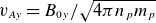 $v_{Ay} = B_{0y}/\sqrt {4\pi n_p m_p}$
. Within the exhaust, due to the strong electric field
$v_{Ay} = B_{0y}/\sqrt {4\pi n_p m_p}$
. Within the exhaust, due to the strong electric field
 $E_x\sim c v_{Ay}/B_0$
, where
$E_x\sim c v_{Ay}/B_0$
, where
 $B_0$
is the guide field, the ion takes up a drift at the Alfvénic outflow velocity
$B_0$
is the guide field, the ion takes up a drift at the Alfvénic outflow velocity
 $v_{out}\sim v_{Ay}$
. If this process happens in a time comparable to the ion’s gyroperiod, the magnetic moment is not conserved and strong heating occurs.
$v_{out}\sim v_{Ay}$
. If this process happens in a time comparable to the ion’s gyroperiod, the magnetic moment is not conserved and strong heating occurs.

Drake et al. (Reference Drake, Swisdak, Phan, Cassak, Shay, Lepri, Lin, Quataert and Zurbuchen2009a ) developed a theory of perpendicular ion heating in reconnection and Drake et al. (Reference Drake, Cassak, Shay, Swisdak and Quataert2009b ) showed that for guide-field reconnection, there was a threshold for strong ion heating by different ion species, namely
 \begin{equation} \frac {m_i/m_p}{Z_i} \sim \frac {1}{2\pi }R^{-1}\beta ^{1/2}\frac {v_{Ay}}{v_{\rm {A}}}, \end{equation}
where
 $R\sim 0.1$
is the normalised reconnection rate
$R\sim 0.1$
is the normalised reconnection rate
 $u_{in}/u_{out}$
,
$u_{in}/u_{out}$
,
 $v_{Ay}$
is the Alfvén speed based on the reconnecting field
$v_{Ay}$
is the Alfvén speed based on the reconnecting field
 $\delta B_y$
, and
$\delta B_y$
, and
 $v_{\textrm{A}}$
is the Alfvén speed based on the guide-field
$v_{\textrm{A}}$
is the Alfvén speed based on the guide-field
 $B_0$
. This was derived in the following way (see figure 4 for a schematic illustration of this scenario). Given a current sheet width of order
$B_0$
. This was derived in the following way (see figure 4 for a schematic illustration of this scenario). Given a current sheet width of order
 $\rho _s= c_s/\varOmega _p$
and an inflow speed
$\rho _s= c_s/\varOmega _p$
and an inflow speed
 $u_{in}\sim R v_{Ay}$
, the transit time of an ion from the inflow out of the sheet is of order
$u_{in}\sim R v_{Ay}$
, the transit time of an ion from the inflow out of the sheet is of order
 $\tau \sim \rho _s/u_{in}$
. Comparing this with the ion’s gyrofrequency
$\tau \sim \rho _s/u_{in}$
. Comparing this with the ion’s gyrofrequency
 $\varOmega _i=\varOmega _p Z_i m_p/m_i$
and requiring
$\varOmega _i=\varOmega _p Z_i m_p/m_i$
and requiring
 $\tau \varOmega _i\lt 1$
gives (5.1). Below the threshold, the ions conserve the first adiabatic invariant
$\tau \varOmega _i\lt 1$
gives (5.1). Below the threshold, the ions conserve the first adiabatic invariant
 $\mu$
, while above the threshold,
$\mu$
, while above the threshold,
 $\mu$
is not conserved and strong ion heating occurs. There is an obvious equivalence between the threshold in
$\mu$
is not conserved and strong ion heating occurs. There is an obvious equivalence between the threshold in
 $\eta _K$
in our estimated heating rate (3.33) and the theory of Drake et al. (Reference Drake, Cassak, Shay, Swisdak and Quataert2009b
). To make this more concrete, we note that in the current sheet, there is an
$\eta _K$
in our estimated heating rate (3.33) and the theory of Drake et al. (Reference Drake, Cassak, Shay, Swisdak and Quataert2009b
). To make this more concrete, we note that in the current sheet, there is an
 $E_x$
driving the Alfvénic exhaust,
$E_x$
driving the Alfvénic exhaust,
 \begin{equation} E_x \sim \frac {B_0 v_{Ay}}{c}, \end{equation}
from which we estimate
 $\varepsilon$
,
$\varepsilon$
,
 \begin{equation} \varepsilon \sim \frac {v_{Ay}}{v_{\rm {th}}}. \end{equation}
For
 $\eta \sim \eta _K\sim \text{const.}$
(we assume this does not vary with
$\eta \sim \eta _K\sim \text{const.}$
(we assume this does not vary with
 $K$
since the outflow is coherent in time), we use the same argument as Drake et al. (Reference Drake, Swisdak, Phan, Cassak, Shay, Lepri, Lin, Quataert and Zurbuchen2009a
), leading to
$K$
since the outflow is coherent in time), we use the same argument as Drake et al. (Reference Drake, Swisdak, Phan, Cassak, Shay, Lepri, Lin, Quataert and Zurbuchen2009a
), leading to
 \begin{equation} \eta \sim \frac {1}{\tau \varOmega _i} \sim 2\pi R\beta ^{-1/2}\frac {m_i/m_p}{Z_i} \frac {v_{Ay}}{v_{\textrm{A}}}. \end{equation}
Applying (3.36) and estimating
 $k_\perp \rho _i\sim k_\perp \rho _s\sim 1$
so that the Bessel function term is of order unity,
$k_\perp \rho _i\sim k_\perp \rho _s\sim 1$
so that the Bessel function term is of order unity,
 \begin{equation} \varDelta T_\perp \sim m_i v_{Ay}^2 \exp \left(-\frac {2}{\eta }\right)\!. \end{equation}
Apart from numerical prefactors of order unity which we have not calculated, this agrees with (6) of Drake et al. (Reference Drake, Swisdak, Phan, Cassak, Shay, Lepri, Lin, Quataert and Zurbuchen2009a
), both in the threshold
 $\eta \sim 1$
and in the order-of-magnitude of the saturated total heating when the threshold is attained. It would also technically be possible to calculate the heating at a reconnection event using our model by specifying the functional form of the electromagnetic fields precisely, arriving at a more accurate estimate; we will leave this for future work.
$\eta \sim 1$
and in the order-of-magnitude of the saturated total heating when the threshold is attained. It would also technically be possible to calculate the heating at a reconnection event using our model by specifying the functional form of the electromagnetic fields precisely, arriving at a more accurate estimate; we will leave this for future work.
This section amounts in some ways to a rederivation of the model of Drake et al. (Reference Drake, Cassak, Shay, Swisdak and Quataert2009b
). However, using our approach, it is perhaps more obvious why the acceleration of the ion into the outflow
 $E\times B$
velocity is accompanied by ion heating. Drake et al. (Reference Drake, Swisdak, Phan, Cassak, Shay, Lepri, Lin, Quataert and Zurbuchen2009a
) suggest that ‘the reflected particles interpenetrate with particles that have already crossed the boundary of the exhaust but have not passed through the reversal region’, thus gaining an effective temperature. In our approach, it is obvious that the diffusion is due to the random initial phase of the particle as it enters the reversal region of the exhaust. While the energy change of each ion
$E\times B$
velocity is accompanied by ion heating. Drake et al. (Reference Drake, Swisdak, Phan, Cassak, Shay, Lepri, Lin, Quataert and Zurbuchen2009a
) suggest that ‘the reflected particles interpenetrate with particles that have already crossed the boundary of the exhaust but have not passed through the reversal region’, thus gaining an effective temperature. In our approach, it is obvious that the diffusion is due to the random initial phase of the particle as it enters the reversal region of the exhaust. While the energy change of each ion
 $\varDelta$
is, on average, zero, considering the plasma distribution function as a whole, the ions acquire a broad range of energies.
$\varDelta$
is, on average, zero, considering the plasma distribution function as a whole, the ions acquire a broad range of energies.
6. Discussion
We have analysed the interaction of an ion with a localised, coherent fluctuation, deriving the change in the ion’s perpendicular and parallel kinetic energy. To lowest order, the energy change is described by (1.1), which depends linearly on the amplitude of the fluctuating fields and on a factor
 $\exp (-1/\eta )$
, where
$\exp (-1/\eta )$
, where
 $\eta \sim 1/\tau \varOmega _i$
, with
$\eta \sim 1/\tau \varOmega _i$
, with
 $\tau$
the characteristic time scale of the fluctuation and
$\tau$
the characteristic time scale of the fluctuation and
 $\varOmega _i$
the ion’s gyrofrequency. For the whole population of ions, the interaction leads to diffusion in energy and heating. This leads to weak heating for
$\varOmega _i$
the ion’s gyrofrequency. For the whole population of ions, the interaction leads to diffusion in energy and heating. This leads to weak heating for
 $\eta \ll 1$
and strong heating for
$\eta \ll 1$
and strong heating for
 $\eta \sim 1$
: this reflects the well-known conservation of the magnetic moment for
$\eta \sim 1$
: this reflects the well-known conservation of the magnetic moment for
 $\eta \ll 1$
and is similar to previous theories of stochastic heating (Chandran et al. Reference Chandran, Li, Rogers, Quataert and Germaschewski2010). As part of our derivation, we have recovered the fact that, if the fluctuation is a wavepacket with a fixed phase velocity
$\eta \ll 1$
and is similar to previous theories of stochastic heating (Chandran et al. Reference Chandran, Li, Rogers, Quataert and Germaschewski2010). As part of our derivation, we have recovered the fact that, if the fluctuation is a wavepacket with a fixed phase velocity
 $v_{\textrm{ph}}$
, the diffusion is along circular scattering contours in
$v_{\textrm{ph}}$
, the diffusion is along circular scattering contours in
 $v_\parallel$
–
$v_\parallel$
–
 $v_\perp$
space, centred on
$v_\perp$
space, centred on
 $v_{\textrm{ph}}$
(§ 3.3), a result usually associated with quasilinear cyclotron resonant heating (Kennel & Engelmann Reference Kennel and Engelmann1966). Thus, our results combine the physics of stochastic heating and cyclotron heating in a single theoretical framework, based on the interaction of ions with coherent structures. In many systems, our approach based on individual localised fluctuations may be more appropriate than the assumption of infinite plane waves usually required to derive the results of quasilinear theory, for example, in strongly nonlinear turbulence and reconnection. The model is also quite easy to apply to different physical situations: one needs estimates for a characteristic time scale relative to the gyroperiod,
$v_{\textrm{ph}}$
(§ 3.3), a result usually associated with quasilinear cyclotron resonant heating (Kennel & Engelmann Reference Kennel and Engelmann1966). Thus, our results combine the physics of stochastic heating and cyclotron heating in a single theoretical framework, based on the interaction of ions with coherent structures. In many systems, our approach based on individual localised fluctuations may be more appropriate than the assumption of infinite plane waves usually required to derive the results of quasilinear theory, for example, in strongly nonlinear turbulence and reconnection. The model is also quite easy to apply to different physical situations: one needs estimates for a characteristic time scale relative to the gyroperiod,
 $1/\eta$
, as well as an estimate of the fluctuation amplitude
$1/\eta$
, as well as an estimate of the fluctuation amplitude
 $\varepsilon$
of the structure.
$\varepsilon$
of the structure.
We have applied our results to low-
 $\beta$
Alfvénic turbulence, obtaining a simple expression for the fraction of the turbulent flux absorbed by the protons in both balanced turbulence and in imbalanced turbulence with a helicity barrier (Meyrand et al. Reference Meyrand, Squire, Schekochihin and Dorland2021), as may be present in the fast Alfvénic solar wind (Bowen et al. Reference Bowen2020; McIntyre et al. Reference McIntyre, Chen, Squire, Meyrand and Simon2024). Our theoretical estimate for the proton heating fraction compares well with the numerically observed estimate for the ion heating fraction of Matthaeus et al. (Reference Matthaeus, Parashar, Wan and Wu2016). We also show that our model is well suited to incorporating different models of intermittency, which we predict should enhance the ion heating: one could also use the observational data to assess this enhancement directly. Moreover, we have determined how the perpendicular length scale of the fluctuation affects the heating rates: at smaller amplitudes, the heating does not peak at
$\beta$
Alfvénic turbulence, obtaining a simple expression for the fraction of the turbulent flux absorbed by the protons in both balanced turbulence and in imbalanced turbulence with a helicity barrier (Meyrand et al. Reference Meyrand, Squire, Schekochihin and Dorland2021), as may be present in the fast Alfvénic solar wind (Bowen et al. Reference Bowen2020; McIntyre et al. Reference McIntyre, Chen, Squire, Meyrand and Simon2024). Our theoretical estimate for the proton heating fraction compares well with the numerically observed estimate for the ion heating fraction of Matthaeus et al. (Reference Matthaeus, Parashar, Wan and Wu2016). We also show that our model is well suited to incorporating different models of intermittency, which we predict should enhance the ion heating: one could also use the observational data to assess this enhancement directly. Moreover, we have determined how the perpendicular length scale of the fluctuation affects the heating rates: at smaller amplitudes, the heating does not peak at
 $k_\perp \rho _{\textrm{th}}\sim 1$
, but at a smaller scale, as was previously observed in the hybrid-kinetic simulations of Arzamasskiy et al. (Reference Arzamasskiy, Kunz, Chandran and Quataert2019). We also show that the heating of minor ions is greatly enhanced over the proton heating, another property associated with both cyclotron (Kasper et al. Reference Kasper, Maruca, Stevens and Zaslavsky2013) and stochastic (Chandran Reference Chandran2010) heating. Our framework can also model ion heating in reconnection, naturally producing perpendicular heating with a threshold similar to the theory and numerical simulations of Drake et al. Reference Drake, Swisdak, Phan, Cassak, Shay, Lepri, Lin, Quataert and Zurbuchen(2009a
,
Reference Drake, Cassak, Shay, Swisdak and Quataertb
). The similarity of our results for heating due to reconnection and turbulence suggest that the disparity between these two paradigms for coronal heating (Chandran & Hollweg Reference Chandran and Hollweg2009; Klimchuk Reference Klimchuk2015) may not be as drastic as often thought.
$k_\perp \rho _{\textrm{th}}\sim 1$
, but at a smaller scale, as was previously observed in the hybrid-kinetic simulations of Arzamasskiy et al. (Reference Arzamasskiy, Kunz, Chandran and Quataert2019). We also show that the heating of minor ions is greatly enhanced over the proton heating, another property associated with both cyclotron (Kasper et al. Reference Kasper, Maruca, Stevens and Zaslavsky2013) and stochastic (Chandran Reference Chandran2010) heating. Our framework can also model ion heating in reconnection, naturally producing perpendicular heating with a threshold similar to the theory and numerical simulations of Drake et al. Reference Drake, Swisdak, Phan, Cassak, Shay, Lepri, Lin, Quataert and Zurbuchen(2009a
,
Reference Drake, Cassak, Shay, Swisdak and Quataertb
). The similarity of our results for heating due to reconnection and turbulence suggest that the disparity between these two paradigms for coronal heating (Chandran & Hollweg Reference Chandran and Hollweg2009; Klimchuk Reference Klimchuk2015) may not be as drastic as often thought.
Johnston et al. (Reference Johnston, Squire and Meyrand2025) have shown within the framework of quasilinear theory that it is possible to recover an exponential or exponential-like suppression of heating, similar to our model and to the original stochastic heating theory of Chandran et al. (Reference Chandran, Li, Rogers, Quataert and Germaschewski2010). Moreover, they show that test-particle heating in both balanced and imbalanced turbulence simulations seems to be well described by such an exponential suppression factor. As reported both by Johnston et al. (Reference Johnston, Squire and Meyrand2025) and in this paper, the exponential factor depends on the typical frequency or inverse time scale of the interactions compared with the ion cyclotron frequency, i.e.
 $\eta \sim 1/\tau \varOmega _i$
, reinforcing the fact that the relevant physics in both cases is the breaking of the magnetic moment conservation. However, the source of the suppression factor is different: Johnston et al. (Reference Johnston, Squire and Meyrand2025) reported that the suppression factor in imbalanced turbulence is due to the steep
$\eta \sim 1/\tau \varOmega _i$
, reinforcing the fact that the relevant physics in both cases is the breaking of the magnetic moment conservation. However, the source of the suppression factor is different: Johnston et al. (Reference Johnston, Squire and Meyrand2025) reported that the suppression factor in imbalanced turbulence is due to the steep
 $k_\parallel$
spectrum outside the critical balance cone leading to very little power at the high resonant frequency, whereas in our case, it comes from the fact that
$k_\parallel$
spectrum outside the critical balance cone leading to very little power at the high resonant frequency, whereas in our case, it comes from the fact that
 $\mu$
is an adiabatic invariant as
$\mu$
is an adiabatic invariant as
 $\eta \to 0$
, conserved to all orders.
$\eta \to 0$
, conserved to all orders.
Acknowledgements
A.M. thanks J. Squire, Z. Johnston and M. Kunz for many useful conversations, and the three referees for insightful comments, which significantly improved this paper.
Editor Nuno Loureiro thanks the referees for their advice in evaluating this article.
Funding
A.M. was supported by NASA grants 80NSSC21K0462 and 80NSSC21K1766. B.C. was supported in part by NASA under grant number 80NSSC24K0171. K.G.K. was partially supported by NASA grant 80NSSC24K0171 and contract 80ARC021C0001. T.E. acknowledges funding from The Chuck Lorre Family Foundation Big Bang Theory Graduate Fellowship and NASA grant 80NSSC20K1285. All authors also acknowledge support from NASA contract NNN06AA01C.
Declaration of interests
The authors report no conflict of interest.
Appendix A. Drifts
As well as calculating the behaviour of the velocity as
 $T\to \infty$
, we might be interested in the drift velocity of the particle at finite
$T\to \infty$
, we might be interested in the drift velocity of the particle at finite
 $T$
. It is easy to see that only the terms with
$T$
. It is easy to see that only the terms with
 $n=0$
in (3.9) and (3.8) contribute to drifts. Integrating the
$n=0$
in (3.9) and (3.8) contribute to drifts. Integrating the
 $n=0$
term of (3.9) by parts,
$n=0$
term of (3.9) by parts,
 \begin{align*} \dot X_{1d} &= \frac {1}{2\pi }\sin T \left \{\left [ \sin T \int _{-\infty }^\infty J_0(K)g(K,0,\eta _K T)\mathrm{d}K\right ]_{-\infty }^T \right .\nonumber \\ &\left .\quad \quad \quad \quad \quad \quad \quad -\int _{-\infty }^T\sin T' \frac {{d}}{\mathrm{d}T'}\int _{-\infty }^\infty J_0(K)g(K,0,\eta _K T)\mathrm{d}K \mathrm{d}T\right \}\nonumber\end{align*}
 \begin{align} &\quad -\frac {1}{2\pi }\cos T \left \{-\left [ \cos T \int _{-\infty }^\infty J_0(K)g(K,0,\eta _K T){\mathrm{d}} K\right ]_{-\infty }^T \right .\nonumber \\ &\left .\quad \quad \quad \quad \quad \quad \quad +\int _{-\infty }^T\cos T' \frac {{d}}{\mathrm{d}T'}\int _{-\infty }^\infty J_0(K)g(K,0,\eta _K T)\mathrm{d}K \mathrm{d}T\right \}\nonumber \\ &= \frac {1}{2\pi }\int _{-\infty }^\infty J_0(K)g(K,0,\eta _K T)\mathrm{d}K\nonumber\\&\quad \quad \quad \quad \quad \quad - \cos T\int _{-\infty }^T\cos T' \frac {{d}}{\mathrm{d}T'}\int _{-\infty }^\infty J_0(K)g(K,0,\eta _K T)\mathrm{d}K \mathrm{d}T \nonumber \\&\quad \quad \quad \quad \quad \quad -\sin T\int _{-\infty }^T\sin T' \frac {{d}}{\mathrm{d}T'}g(0,0,\eta _K T')\mathrm{d}T. \end{align}
The first term is the gyroaveraged
 $E\times B$
drift velocity. Repeating the integration by parts,
$E\times B$
drift velocity. Repeating the integration by parts,
 \begin{align} \dot X_{1d} &= \frac {1}{2\pi }\int _{-\infty }^\infty J_0(K)g(K,0,\eta _K T)\mathrm{d}K\nonumber \\ &\quad - \frac {1}{2\pi }\cos T \left \{ \left [\sin T \frac {{\rm d}}{\mathrm{d}T'}\int _{-\infty }^\infty J_0(K)g(K,0,\eta _K T)\mathrm{d}K\right ]_{-\infty }^T \nonumber \right .\\ &\left .\quad \quad \quad \quad \quad \quad - \int _{-\infty }^T \sin T' \frac {{\rm d}^2}{\mathrm{d}{T'}^2} \int _{-\infty }^\infty J_0(K)g(K,0,\eta _K T)\mathrm{d}K\,\mathrm{d}T' \right \} \nonumber \\ &\quad + \frac {1}{2\pi }\sin T \left \{ \left [\cos T \frac {{\rm d}}{\mathrm{d}T'}\int _{-\infty }^\infty J_0(K)g(K,0,\eta _K T)\,{\rm d}K\right ]_{-\infty }^T \nonumber \right .\\ &\left .\quad \quad \quad \quad \quad \quad - \int _{-\infty }^T \cos T' \frac {\mathrm{d}^2}{\mathrm{d}{T'}^2} \int _{-\infty }^\infty J_0(K)g(K,0,\eta _K T)\mathrm{d}K\, \mathrm{d}T' \right \} \nonumber \\ &= \frac {1}{2\pi }\int _{-\infty }^\infty J_0(K)g(K,0,\eta _K T)\mathrm{d}K \nonumber \\&\quad \quad + \frac {1}{2\pi }\cos T \int _{-\infty }^T \sin T'\frac {{d}^2}{\mathrm{d}{T'}^2} \int _{-\infty }^\infty J_0(K)g(K,0,\eta _K T)\mathrm{d}K\,\mathrm{d}T' \nonumber \\& \quad \quad - \frac {1}{2\pi }\sin T\int _{-\infty }^T \cos T'\frac {\mathrm{d}^2}{\mathrm{d}{T'}^2} \int _{-\infty }^\infty J_0(K)g(K,0,\eta _K T)\mathrm{d}K\,\mathrm{d}T'. \end{align}
Comparing this and (3.9), it is easy to see the pattern:
 \begin{align} \dot X_{1d} &= \frac {1}{2\pi }\sum _{m=0}^M (-1)^m\frac {{\rm d}^{2m}}{\mathrm{d}T^{2m}}\int _{-\infty }^\infty J_0(K)g(K,0,\eta _K T)\mathrm{d}K \nonumber \\ &\quad + \frac {(-1)^{M+1}}{2\pi }\cos T \int _{-\infty }^T\sin T' \frac {{\rm d}^{2M+2}}{\mathrm{d}{T'}^{2M+2}}\int _{-\infty }^\infty J_0(K)g(K,0,\eta _K T)\mathrm{d}K \,\mathrm{d}T'\nonumber \\ &\quad - \frac {(-1)^{M+1}}{2\pi }\sin T \int _{-\infty }^T\cos T' \frac {\mathrm{d}^{2M+2}}{\mathrm{d}{T'}^{2M+2}}\int _{-\infty }^\infty J_0(K)g(K,0,\eta _K T)\mathrm{d}K \,\mathrm{d}T', \end{align}
a series of corrections to the lowest-order gyroaveraged
 $\boldsymbol{E}\times {\boldsymbol{B}}$
velocity (Stephens, Brzozowski & Jenko Reference Stephens, Brzozowski and Jenko2017). Taking
$\boldsymbol{E}\times {\boldsymbol{B}}$
velocity (Stephens, Brzozowski & Jenko Reference Stephens, Brzozowski and Jenko2017). Taking
 $M\to \infty$
, we obtain the infinite series
$M\to \infty$
, we obtain the infinite series
 \begin{equation} \dot X_{1d} = \frac {1}{2\pi }\sum _{m=0}^\infty (-1)^m\frac {\mathrm{d}^{2m}}{\mathrm{d}T^{2m}}\int _{-\infty }^\infty J_0(K)\tilde {g}(K,0,\eta _K T)\mathrm{d}K. \end{equation}
Differentiating, we obtain a similar series for the drifts in the
 $\hat {\boldsymbol{y}}$
direction,
$\hat {\boldsymbol{y}}$
direction,
 \begin{equation} \dot Y_{1d} = \frac {1}{2\pi }\sum _{m=0}^\infty (-1)^m\frac {\mathrm{d}^{2m+1}}{\mathrm{d}T^{2m+1}}\int _{-\infty }^\infty J_0(K)\tilde {g}(K,0,\eta _K T)\mathrm{d}K, \end{equation}
with the first term being the gyroaveraged polarisation drift. For
 $\eta \ll 1$
, each successive term in the sum is smaller than the next by a factor
$\eta \ll 1$
, each successive term in the sum is smaller than the next by a factor
 $\sim \eta ^2$
. If
$\sim \eta ^2$
. If
 $\eta \sim 1$
, drifts at all orders are comparable and the series does not converge. As
$\eta \sim 1$
, drifts at all orders are comparable and the series does not converge. As
 $T\to \infty$
, the drift part of the motion vanishes since we required
$T\to \infty$
, the drift part of the motion vanishes since we required
 $g(y,z,\infty )=0$
.
$g(y,z,\infty )=0$
.
Appendix B. Resonance
We could modify the example in § 3.4 by multiplying by a sinusoid,
 \begin{equation} \tilde {g}(K,0,\eta _K T) = \frac {1}{\pi }\tilde {h}(K)\cos \left (\nu t + \phi \right )\left \{\arctan [\eta _K(T-a)]-\arctan [\eta _K(T-b)]\right\}\!. \end{equation}
Expanding the products of cosines and sines appearing in the integral solution for
 $\varDelta$
(3.14), we find that there are terms in the integrands multiplied by
$\varDelta$
(3.14), we find that there are terms in the integrands multiplied by
 $\exp [\pm i(\nu \pm 1)t]$
. For
$\exp [\pm i(\nu \pm 1)t]$
. For
 $\nu = \pm 1$
, secular terms therefore appear in the solution for
$\nu = \pm 1$
, secular terms therefore appear in the solution for
 $\dot Y_1$
, scaling with the time interval over which the sinusoidally varying fields are applied. If
$\dot Y_1$
, scaling with the time interval over which the sinusoidally varying fields are applied. If
 $b-a \gtrsim 1/\varepsilon$
, then
$b-a \gtrsim 1/\varepsilon$
, then
 $\dot Y_1\gtrsim 1$
in this resonant case. However, in practice, this type of fluctuation clearly involves an overall rate of change of the fields
$\dot Y_1\gtrsim 1$
in this resonant case. However, in practice, this type of fluctuation clearly involves an overall rate of change of the fields
 $\eta ' \sim 1$
, so that
$\eta ' \sim 1$
, so that
 $\exp (-1/\eta ')\sim 1$
and in terms of scalings, the possibility of this resonant type of fluctuation makes little difference to the end result. In the rest of the paper, we ignore this subtlety and assume that our fluctuation is not resonant.
$\exp (-1/\eta ')\sim 1$
and in terms of scalings, the possibility of this resonant type of fluctuation makes little difference to the end result. In the rest of the paper, we ignore this subtlety and assume that our fluctuation is not resonant.
Appendix C. The case with
$\eta _K\sim \varepsilon$

Examining our expressions for
 $\dot {X}_1$
and
$\dot {X}_1$
and
 $\dot {Y}_1$
(see (3.10)–(3.11)), it is possible to see that in fact, the coefficient with
$\dot {Y}_1$
(see (3.10)–(3.11)), it is possible to see that in fact, the coefficient with
 $n=0$
resulting from the second line does not vanish. As mentioned in the main paper, this means that if the fluctuating field is applied over a time longer than
$n=0$
resulting from the second line does not vanish. As mentioned in the main paper, this means that if the fluctuating field is applied over a time longer than
 $O(1/\varepsilon )$
, our ordering in
$O(1/\varepsilon )$
, our ordering in
 $\varepsilon$
breaks down, since this secular term will become large. This is not a true resonance, however, and results from the fact that our expansion procedure does not take into account the nearly periodic nature of the system.
$\varepsilon$
breaks down, since this secular term will become large. This is not a true resonance, however, and results from the fact that our expansion procedure does not take into account the nearly periodic nature of the system.
To illustrate the issue, we first consider a simplified example. Suppose that the electric field is given by
 $g(Y,Z,T) = Y$
, constant in time, but depending on
$g(Y,Z,T) = Y$
, constant in time, but depending on
 $Y$
. Then, our equation for
$Y$
. Then, our equation for
 $Y$
is
$Y$
is
 \begin{equation} \ddot Y + Y = \epsilon Y. \end{equation}
This has the exact solution
 $Y=\sin [(1-\varepsilon )T]$
, i.e. the variation of the electric field in space has introduced a frequency shift (Stephens et al. Reference Stephens, Brzozowski and Jenko2017). Now, suppose we instead attempted to expand in
$Y=\sin [(1-\varepsilon )T]$
, i.e. the variation of the electric field in space has introduced a frequency shift (Stephens et al. Reference Stephens, Brzozowski and Jenko2017). Now, suppose we instead attempted to expand in
 $\varepsilon$
: we would instead get
$\varepsilon$
: we would instead get
 $Y_0=\sin T$
and, at first order,
$Y_0=\sin T$
and, at first order,
 \begin{equation} \ddot {Y}_1 + Y_1 = Y_0 =\sin T, \end{equation}
which is secular. To avoid this, we can use the Poincaré–Lindstedt method (Bender & Orszag Reference Bender and Orszag2013), introducing a stretched time variable
 $\tau =pT$
, with
$\tau =pT$
, with
 \begin{equation} p = 1 + \varepsilon p_1 + \varepsilon ^2 p_2 +\ldots \end{equation}
Now, at first order, we have
 \begin{align} \ddot {Y}_1 +Y_1 &= Y_0-2p_1\ddot {Y}_0, \end{align}
 \begin{align} \ddot {Y}_1 + Y_1 &= (1+2p_1)\sin T,\\[6pt] \nonumber \end{align}
where we have, in an abuse of notation, redefined the overdot to mean differentiation by
 $\tau$
. The solution that avoids a secular term is
$\tau$
. The solution that avoids a secular term is
 $p_1 = -1/2$
, which agrees with the exact solution up to first order in
$p_1 = -1/2$
, which agrees with the exact solution up to first order in
 $\varepsilon$
.
$\varepsilon$
.
Our problem unfortunately does not have an readily available exact solution, but we can still apply the Poincaré–Lindstedt method. We order
 $\eta _K\sim \varepsilon$
. Because of the time dependence of the electromagnetic fields, the stretching of time variable
$\eta _K\sim \varepsilon$
. Because of the time dependence of the electromagnetic fields, the stretching of time variable
 $\tau =pT$
now itself depends slowly on time, with
$\tau =pT$
now itself depends slowly on time, with
 \begin{equation} p = 1 + \varepsilon p_1(\varepsilon T) + \varepsilon ^2 p_2 (\varepsilon T) +\ldots \end{equation}
Our differential equation for
 $Y_1$
(replacing (3.3)) becomes
$Y_1$
(replacing (3.3)) becomes
 \begin{equation} \ddot {Y}_1 + Y_1 = g(\sin \tau , 0 , T) -2p_1\sin \tau . \end{equation}
This may be solved (as before) by Fourier transforming in time and back again, and the solution for the velocity is
 \begin{equation} \dot {Y}_1 = \int _{-\infty }^\tau \cos (\tau -\tau ')\left [g(\sin \tau ',0,\tau ') + 2p_1\sin \tau '\right ]\,\mathrm{d}\tau '. \end{equation}
Following the same procedure as in § 3, (see (3.6)–(3.10)) (Fourier transforming in
 $Y$
according to (2.5), applying the Bessel function identity (3.7), and expanding the cosine and combining the resulting sinusoidal terms in the integrands), we obtain
$Y$
according to (2.5), applying the Bessel function identity (3.7), and expanding the cosine and combining the resulting sinusoidal terms in the integrands), we obtain
 \begin{align} \dot {Y}_1 &= \frac {1}{2\pi }\cos \tau \int _{-\infty }^\tau \int _{-\infty }^\infty g(K,0,\eta _K\tau ')\sum _{n=-\infty }^\infty \frac {nJ_n(K)}{K}e^{in\tau '}\,{\rm d}K + p_1\sin 2\tau '\,{\rm d}\tau '\nonumber \\ &\quad \,+\frac {1}{2\pi }\sin \tau \int _{-\infty }^\tau \int _{-\infty }^\infty g(K,0,\eta _K\tau ')\sum _{n=-\infty }^\infty \frac {J_{n-1}(K)-J_{n+1}(K)}{2i}e^{in\tau '}\,{\rm d}K\nonumber \\ &\quad \quad \quad \quad \quad \quad \quad \quad \quad \quad \quad + p_1(1-\cos 2\tau ')\,{\rm d}\tau '. \end{align}
A secular term would result if there were a non-zero term in the
 $\tau '$
integrand of (C9) with no sinusoidal variation – as discussed previously, such a term would break the ordering of our solution if the electric field
$\tau '$
integrand of (C9) with no sinusoidal variation – as discussed previously, such a term would break the ordering of our solution if the electric field
 $g$
remains ‘on’ for a time of order
$g$
remains ‘on’ for a time of order
 $1/\varepsilon$
. In the second integral of (C9), one such term results from the
$1/\varepsilon$
. In the second integral of (C9), one such term results from the
 $n=0$
term, while there is another in the
$n=0$
term, while there is another in the
 $p_1$
term. To ensure they cancel, we choose
$p_1$
term. To ensure they cancel, we choose
 \begin{equation} p_1 = -i\int _{-\infty }^\infty J_1(K) \tilde {g}(K,0,\eta _K\tau ) \,{\rm d}K = \int _0^\infty J_1(K) \mathrm{Im}[\tilde {g}(K,0,\eta _K\tau )]\, {\rm d}K, \end{equation}
where the second equality follows since the electric field is real; thus,
 $p_1$
is real. Because
$p_1$
is real. Because
 $J_1(K)\approx K/2$
for
$J_1(K)\approx K/2$
for
 $K\ll 1$
, if
$K\ll 1$
, if
 $g$
varies only on large scales,
$g$
varies only on large scales,
 \begin{equation} p_1 \approx -\left .\frac {1}{2}\frac {{\rm d}g}{{\rm d}Y}\right |_{Y,Z=0}. \end{equation}
This agrees with our previous simplified example with
 $g=Y$
. In other words, if the electric field varies only a small amount over the gyroradius of the particle,
$g=Y$
. In other words, if the electric field varies only a small amount over the gyroradius of the particle,
 $p_1$
will also be small (by a factor
$p_1$
will also be small (by a factor
 $k_\perp \rho$
).
$k_\perp \rho$
).
With this analysis, it is now proven that even when
 $\eta _K\sim \varepsilon$
or smaller,
$\eta _K\sim \varepsilon$
or smaller,
 $\dot {Y}_1$
(and
$\dot {Y}_1$
(and
 $\dot {X}_1$
, by identical arguments) are exponentially small as
$\dot {X}_1$
, by identical arguments) are exponentially small as
 $T\to \infty$
, as is
$T\to \infty$
, as is
 $\varDelta$
.
$\varDelta$
.


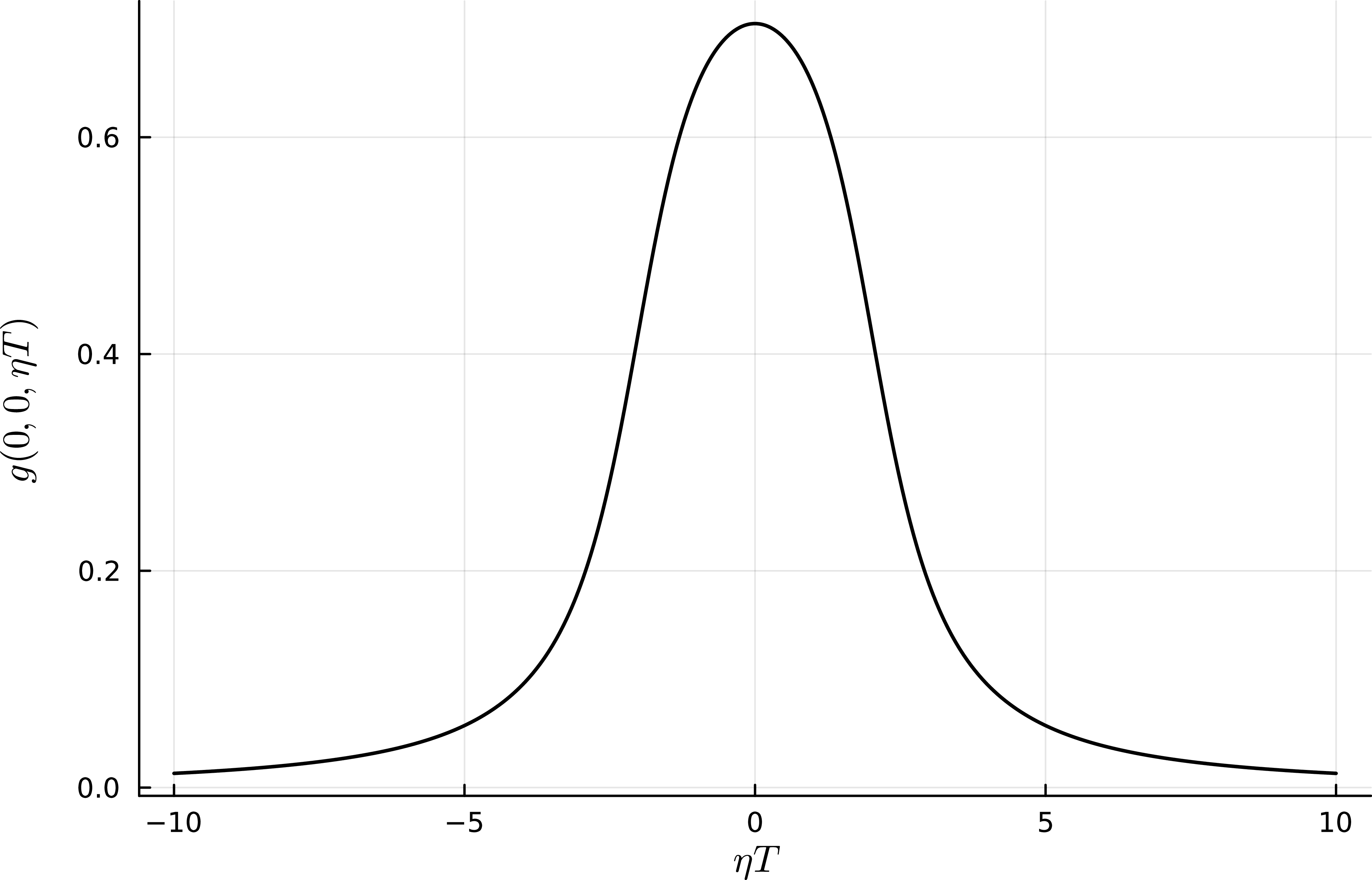


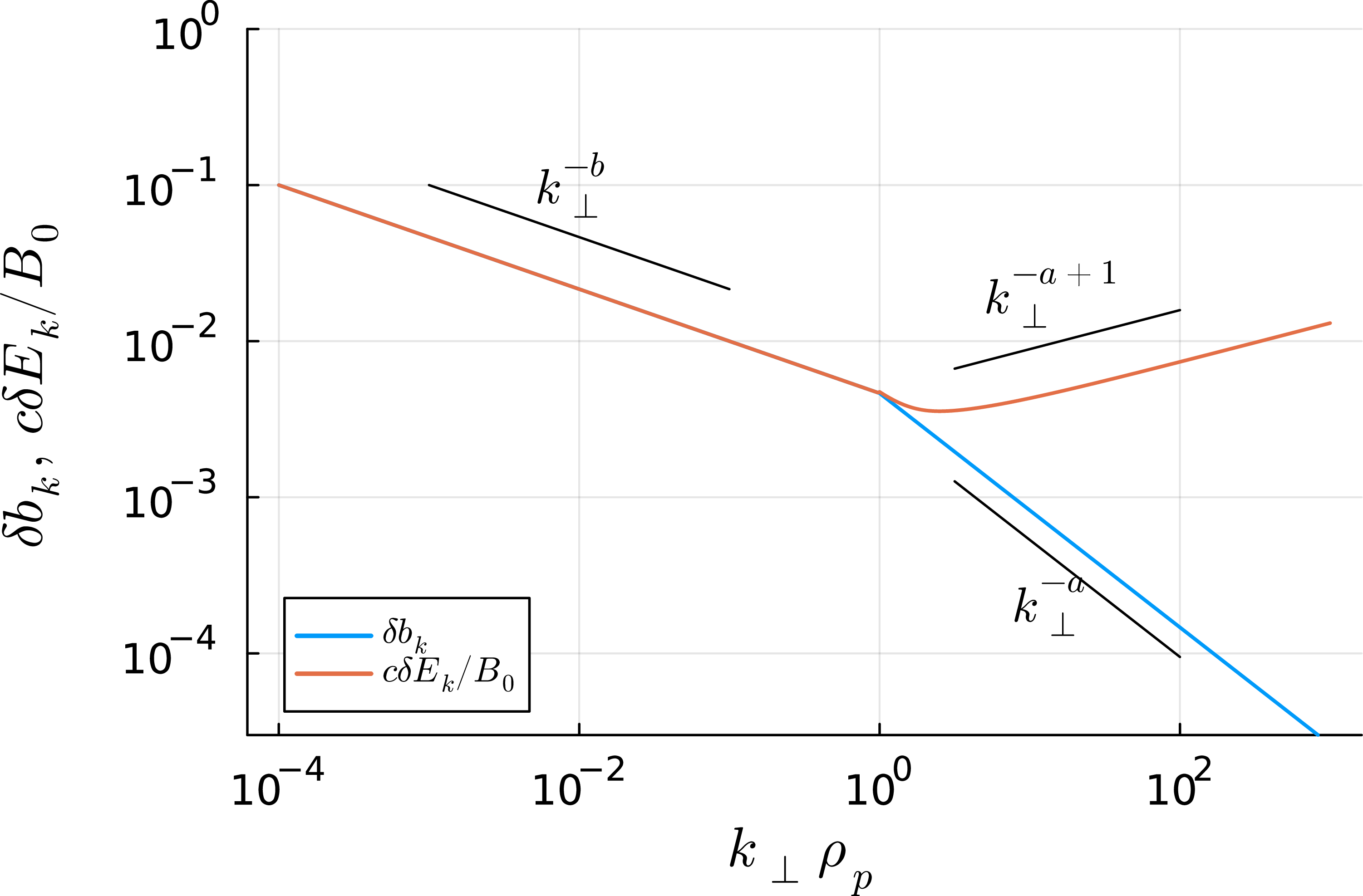


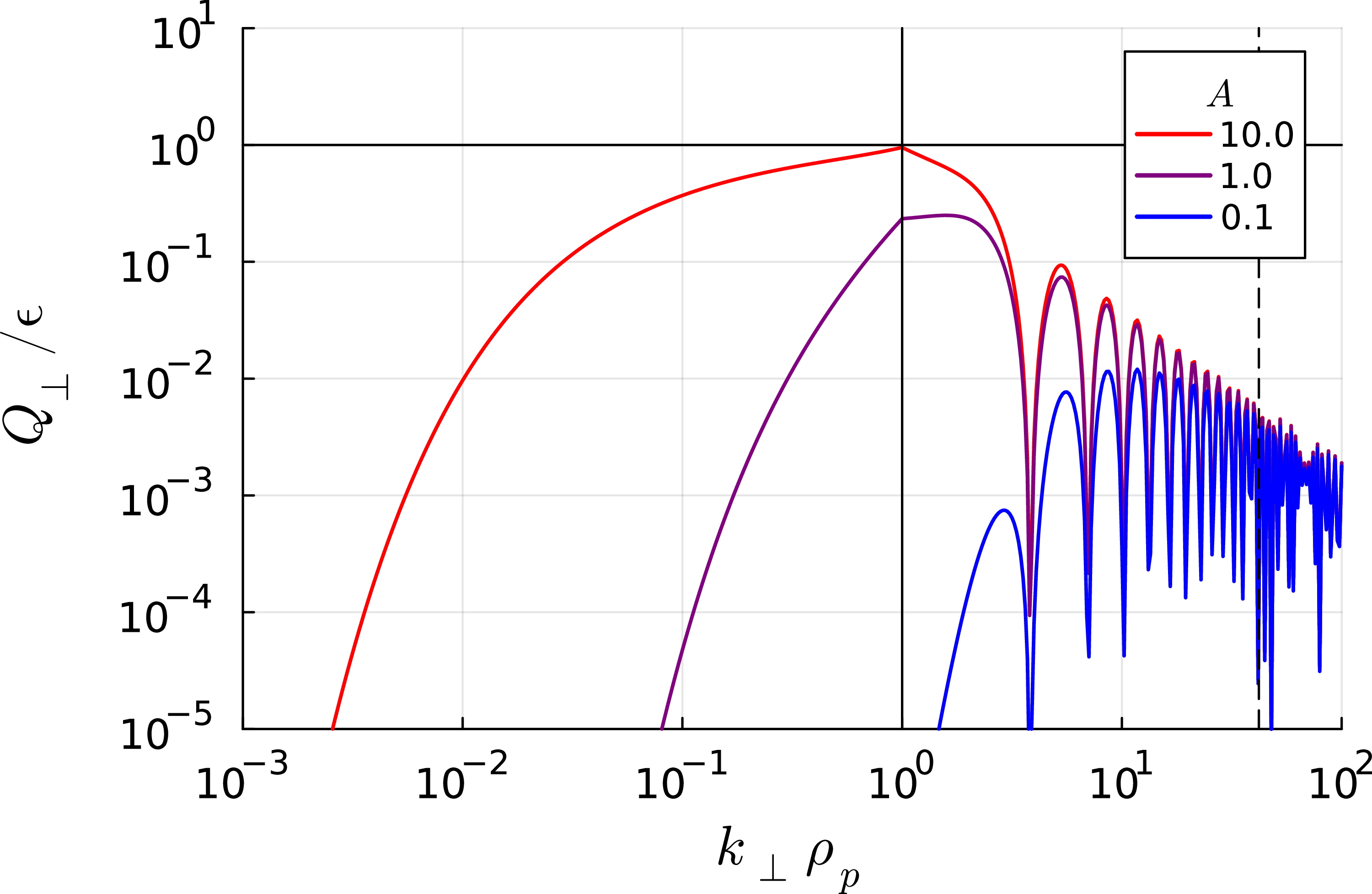


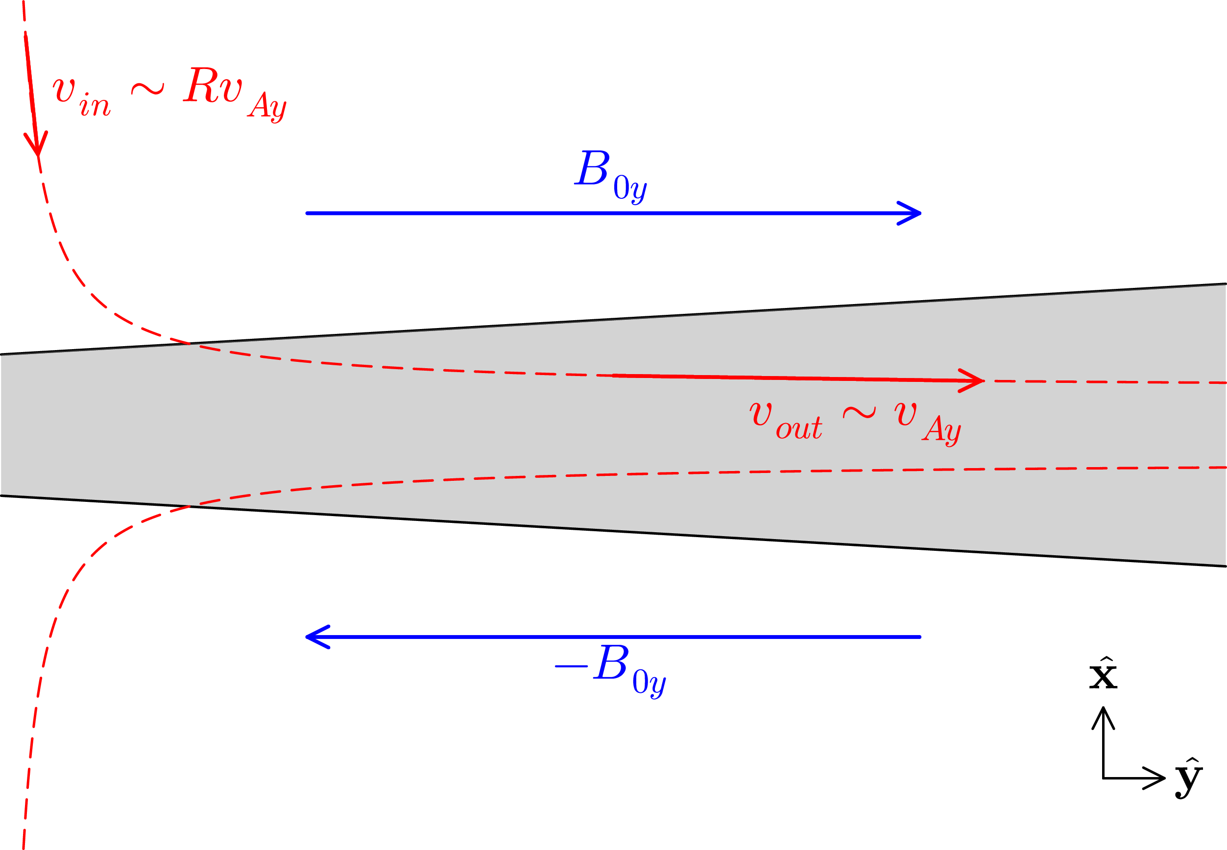


 Open access