





1. Introduction
Mass transfer in drop-/bubble-laden turbulent flows is a key process in a wide range of fields, from environmental and atmospheric sciences (Emerson & Bushinsky Reference Emerson and Bushinsky2016; Deike Reference Deike2022) to process engineering (Kokal Reference Kokal2005; Risso Reference Risso2018). Examples include oxygenation in water bodies, carbon dioxide ( $\text{CO}_2$
) absorption and pollutant removal – influencing aquatic ecosystems and climate regulation – but also mixing in chemical reactors, two-phase heat exchangers and emulsions (Pelusi et al. Reference Pelusi, Ascione, Sbragaglia and Bernaschi2023). Whether in the upper layers of the ocean, or in a chemical reactor, the presence of drops/bubbles in a turbulent flow significantly influences the efficiency of mass transfer between phases (Xu et al. Reference Xu, Tan, Li and Luo2008). The problem of mass transfer in drop-/bubble-laden turbulence is, however, extremely complicated to study. Beyond the complexity of capturing the dynamics of the turbulent carrier phase in large-scale inherently inhomogeneous flows (which is itself rather challenging) we have to consider the presence of a second dispersed phase – i.e. a drop – with its own thermophysical/physicochemical properties, which can indeed be very different compared with those of the carrier phase. In addition, the two phases are separated by an interface that can deform according to the behaviour of the surrounding turbulent flow, and that can change topology (i.e. coalescence and breakage events). It is therefore not surprising that the characterisation of the mass transfer at a fluid interface requires the evaluation of many parameters, the most important of which are the Reynolds number
$\text{CO}_2$
) absorption and pollutant removal – influencing aquatic ecosystems and climate regulation – but also mixing in chemical reactors, two-phase heat exchangers and emulsions (Pelusi et al. Reference Pelusi, Ascione, Sbragaglia and Bernaschi2023). Whether in the upper layers of the ocean, or in a chemical reactor, the presence of drops/bubbles in a turbulent flow significantly influences the efficiency of mass transfer between phases (Xu et al. Reference Xu, Tan, Li and Luo2008). The problem of mass transfer in drop-/bubble-laden turbulence is, however, extremely complicated to study. Beyond the complexity of capturing the dynamics of the turbulent carrier phase in large-scale inherently inhomogeneous flows (which is itself rather challenging) we have to consider the presence of a second dispersed phase – i.e. a drop – with its own thermophysical/physicochemical properties, which can indeed be very different compared with those of the carrier phase. In addition, the two phases are separated by an interface that can deform according to the behaviour of the surrounding turbulent flow, and that can change topology (i.e. coalescence and breakage events). It is therefore not surprising that the characterisation of the mass transfer at a fluid interface requires the evaluation of many parameters, the most important of which are the Reynolds number ${\textit{Re}}$
, a measure of the inertia to viscous forces ratio, the Weber number
${\textit{Re}}$
, a measure of the inertia to viscous forces ratio, the Weber number ${\textit{We}}$
, a measure of the inertia to surface tension forces ratio, the Schmidt number
${\textit{We}}$
, a measure of the inertia to surface tension forces ratio, the Schmidt number ${\textit{Sc}}$
, a measure of the momentum to mass diffusivity ratio, and the Sherwood number
${\textit{Sc}}$
, a measure of the momentum to mass diffusivity ratio, and the Sherwood number ${\textit{Sh}}$
, a measure of the mass-transfer rate. Note that, in particular in the context of geophysical/environmental applications,
${\textit{Sh}}$
, a measure of the mass-transfer rate. Note that, in particular in the context of geophysical/environmental applications, ${\textit{Sh}}$
is often replaced by the gas transfer velocity,
${\textit{Sh}}$
is often replaced by the gas transfer velocity, $\mathcal{K}\sim {Sh}/Sc$
. Because of the many practical applications, the literature in the field of mass transfer through interfaces is vast, and can be dated back to the seminal work of Boussinesq (Reference Boussinesq1905) and Levich (Reference Levich1962) on theoretical/analytical prediction of the mass transfer at the interface of an isolated bubble rising in a quiescent liquid. Many other semi-empirical/analytical studies have followed (see Kumar & Hartland (Reference Kumar and Hartland1999) for a comprehensive review), which typically apply to simplified cases of isolated/undeformable drops/bubbles immersed in quiescent or steady flows, and usually provide the value of
$\mathcal{K}\sim {Sh}/Sc$
. Because of the many practical applications, the literature in the field of mass transfer through interfaces is vast, and can be dated back to the seminal work of Boussinesq (Reference Boussinesq1905) and Levich (Reference Levich1962) on theoretical/analytical prediction of the mass transfer at the interface of an isolated bubble rising in a quiescent liquid. Many other semi-empirical/analytical studies have followed (see Kumar & Hartland (Reference Kumar and Hartland1999) for a comprehensive review), which typically apply to simplified cases of isolated/undeformable drops/bubbles immersed in quiescent or steady flows, and usually provide the value of ${\textit{Sh}}$
based on the specific flow configuration and on the value of
${\textit{Sh}}$
based on the specific flow configuration and on the value of ${\textit{Re}}$
and
${\textit{Re}}$
and ${\textit{Sc}}$
. Semi-empirical/analytical approaches are naturally not possible for large numbers of drops/bubbles. In such cases, the most common approach is to consider many small undeformable drops/bubbles of sub-Kolmogorov size, which are dispersed into the flow and are tracked as material points via a Lagrangian approach (Kuerten Reference Kuerten2016). When the drops/bubbles are large and are immersed in a turbulent flow, the problem becomes much more complicated, since the drops/bubbles can change shape and topology according to the external turbulent flow field. Even in this case, semi-analytical and theoretical predictions are not very reliable, and accurate experiments are particularly challenging to perform. Only recently, and because of the development of laser-induced fluorescence methods and similar optical techniques, experimental measurements of mass-transfer processes in bubble-laden turbulence have become available (Dani, Guiraud & Cockx Reference Dani, Guiraud and Cockx2007; Francois et al. Reference Francois, Dietrich, Guiraud and Cockx2011; Colombet et al. Reference Colombet, Legendre, Cockx, Guiraud, Risso, Daniel and Galinat2011, Reference Colombet, Legendre, Risso, Cockx and Guiraud2015). These techniques are, however, generally suitable for providing insightful information on integral/global quantities only, given the intrinsic difficulty in capturing the distribution of scalar concentration and gradients at fluid interfaces that can deform, break and coalesce. For this reason, high-fidelity numerical simulations remain particularly attractive (see e.g. Méès et al. Reference Méès, Grosjean, Marié and Fournier2020; Dodd et al. Reference Dodd, Mohaddes, Ferrante and Ihme2021; Scapin et al. Reference Scapin, Barba, Federico, Giandomenico, Edoardo, Duwig and Brandt2022; Hidman et al. Reference Hidman, Ström, Sasic and Sardina2023). Nevertheless, most of these simulations focus on a single drop/bubble immersed in a turbulent flow, with the remarkable exception of the work by Hidman et al. (Reference Hidman, Ström, Sasic and Sardina2023), which focused on the transport of a passive scalar, subject to an externally imposed mean scalar gradient, in an unbounded, bubble-induced turbulent flow, in which bubble coalescence/interaction is prevented. To the best of our knowledge, there is no systematic study on the problem of mass transport in drop-laden wall-bounded turbulence, and focusing in particular on the influence of the diffusivity ratio between drops/bubbles and carrier flow. With the present study, we start bridging this gap. Specifically, we consider a drop-laden turbulent channel flow, and we perform a series of direct numerical simulations (DNS) of the mass-transfer process occurring between the drops and the turbulent carrier flow. Simulations are run using an incompressible Navier–Stokes solver coupled with a volume-of-fluid (VOF) method tailored for tracking the dynamics of the drop interface. Central in our study is the modelling of the species transport within the flow, which we have accomplished via the definition of an ad hoc advection–diffusion equation. This equation is suitable to account for different diffusivity and solubility between the two phases (drops and carrier flow) and to incorporate the solubility of the solute within the carrier phase. Overall, the employed methodology allows for a detailed evaluation of the interfacial mass transfer and a detailed analysis of the underlying physical processes influencing it, providing new insights into the mass-transfer process in turbulent multiphase flows.
${\textit{Sc}}$
. Semi-empirical/analytical approaches are naturally not possible for large numbers of drops/bubbles. In such cases, the most common approach is to consider many small undeformable drops/bubbles of sub-Kolmogorov size, which are dispersed into the flow and are tracked as material points via a Lagrangian approach (Kuerten Reference Kuerten2016). When the drops/bubbles are large and are immersed in a turbulent flow, the problem becomes much more complicated, since the drops/bubbles can change shape and topology according to the external turbulent flow field. Even in this case, semi-analytical and theoretical predictions are not very reliable, and accurate experiments are particularly challenging to perform. Only recently, and because of the development of laser-induced fluorescence methods and similar optical techniques, experimental measurements of mass-transfer processes in bubble-laden turbulence have become available (Dani, Guiraud & Cockx Reference Dani, Guiraud and Cockx2007; Francois et al. Reference Francois, Dietrich, Guiraud and Cockx2011; Colombet et al. Reference Colombet, Legendre, Cockx, Guiraud, Risso, Daniel and Galinat2011, Reference Colombet, Legendre, Risso, Cockx and Guiraud2015). These techniques are, however, generally suitable for providing insightful information on integral/global quantities only, given the intrinsic difficulty in capturing the distribution of scalar concentration and gradients at fluid interfaces that can deform, break and coalesce. For this reason, high-fidelity numerical simulations remain particularly attractive (see e.g. Méès et al. Reference Méès, Grosjean, Marié and Fournier2020; Dodd et al. Reference Dodd, Mohaddes, Ferrante and Ihme2021; Scapin et al. Reference Scapin, Barba, Federico, Giandomenico, Edoardo, Duwig and Brandt2022; Hidman et al. Reference Hidman, Ström, Sasic and Sardina2023). Nevertheless, most of these simulations focus on a single drop/bubble immersed in a turbulent flow, with the remarkable exception of the work by Hidman et al. (Reference Hidman, Ström, Sasic and Sardina2023), which focused on the transport of a passive scalar, subject to an externally imposed mean scalar gradient, in an unbounded, bubble-induced turbulent flow, in which bubble coalescence/interaction is prevented. To the best of our knowledge, there is no systematic study on the problem of mass transport in drop-laden wall-bounded turbulence, and focusing in particular on the influence of the diffusivity ratio between drops/bubbles and carrier flow. With the present study, we start bridging this gap. Specifically, we consider a drop-laden turbulent channel flow, and we perform a series of direct numerical simulations (DNS) of the mass-transfer process occurring between the drops and the turbulent carrier flow. Simulations are run using an incompressible Navier–Stokes solver coupled with a volume-of-fluid (VOF) method tailored for tracking the dynamics of the drop interface. Central in our study is the modelling of the species transport within the flow, which we have accomplished via the definition of an ad hoc advection–diffusion equation. This equation is suitable to account for different diffusivity and solubility between the two phases (drops and carrier flow) and to incorporate the solubility of the solute within the carrier phase. Overall, the employed methodology allows for a detailed evaluation of the interfacial mass transfer and a detailed analysis of the underlying physical processes influencing it, providing new insights into the mass-transfer process in turbulent multiphase flows.
In agreement with previous theoretical predictions (Bird Reference Bird2002; Wylock, Colinet & Haut Reference Wylock, Colinet and Haut2012), we show that different regimes for mass transport at a deformable interface are possible, which depend on the dispersed phase (subscript ‘d’) to carrier fluid (subscript ‘c’) diffusivity ratio $D_r=D_d/D_c$
(assuming a unitary equilibrium concentration ratio across the interface,
$D_r=D_d/D_c$
(assuming a unitary equilibrium concentration ratio across the interface, $\alpha =C^{eq}_b/C^{eq}_c=1$
). Attention is here focused at the regime in which the mass-transport resistance inside the drop has little influence,
$\alpha =C^{eq}_b/C^{eq}_c=1$
). Attention is here focused at the regime in which the mass-transport resistance inside the drop has little influence, $ \sqrt {D_r}\gg 1$
, and at the coupled regime,
$ \sqrt {D_r}\gg 1$
, and at the coupled regime, $ \sqrt {D_r}\simeq 1$
, in which the mass-transport resistance in both phases is important. A third regime,
$ \sqrt {D_r}\simeq 1$
, in which the mass-transport resistance in both phases is important. A third regime, $ \sqrt {D_r}\ll 1$
, in which the mass-transport resistance outside of the drop has little influence, would be possible, though not of interest in the context of the present work.
$ \sqrt {D_r}\ll 1$
, in which the mass-transport resistance outside of the drop has little influence, would be possible, though not of interest in the context of the present work.
2. Methodology
The DNS of turbulence is coupled with the VOF method to study the mass-transfer process in a drop-laden turbulent Poiseuille channel flow. In dimensionless form, the governing equations are
 \begin{align} \frac {\partial \chi }{\partial t} + \boldsymbol{u} \boldsymbol{\cdot }\boldsymbol{\nabla }\chi &= 0,\end{align}
 \begin{align} \boldsymbol{\nabla }\boldsymbol{\cdot }\boldsymbol{u} &= 0,\end{align}
 \begin{align} \frac { \partial \boldsymbol{u} } { \partial t} + \boldsymbol{\nabla }\boldsymbol{\cdot }\left (\boldsymbol{uu}\right ) &= \frac {1}{\rho } \left [ -\boldsymbol{\nabla }p + \frac {1}{\textit{Re}} \boldsymbol{\nabla }\boldsymbol{\cdot }\left ( \mu \left ( \boldsymbol{\nabla }\boldsymbol{u}+ \boldsymbol{\nabla }\boldsymbol{u}^T \right ) \right ) + \frac {1}{{We}} \boldsymbol{f}_{\sigma } \right ] + \varPi \boldsymbol{i},\end{align}
where $\chi$
is the phase indicator,
$\chi$
is the phase indicator, $\boldsymbol{u} = \boldsymbol{u} (\boldsymbol{x}, t )$
is the fluid velocity,
$\boldsymbol{u} = \boldsymbol{u} (\boldsymbol{x}, t )$
is the fluid velocity, $p = p ( \boldsymbol{x}, t )$
is the pressure,
$p = p ( \boldsymbol{x}, t )$
is the pressure, $\rho = \rho ( \boldsymbol{x}, t )$
is the density,
$\rho = \rho ( \boldsymbol{x}, t )$
is the density, $\mu = \mu ( \boldsymbol{x}, t )$
is the dynamic viscosity,
$\mu = \mu ( \boldsymbol{x}, t )$
is the dynamic viscosity, $\boldsymbol{f}_{\sigma }$
is the surface tension force and
$\boldsymbol{f}_{\sigma }$
is the surface tension force and $\varPi$
is the pressure gradient applied to keep constant the mass flow rate along the streamwise direction (versor
$\varPi$
is the pressure gradient applied to keep constant the mass flow rate along the streamwise direction (versor $\boldsymbol{i}$
). The surface tension force is modelled as a volumetric force (continuum surface force model) concentrated at the interface:
$\boldsymbol{i}$
). The surface tension force is modelled as a volumetric force (continuum surface force model) concentrated at the interface:
 \begin{equation} \boldsymbol{f}_{\sigma } = k \delta _D \left ( \boldsymbol{x} - \boldsymbol{x}_s \right ) \boldsymbol{n}, \end{equation}
where $\boldsymbol{n}$
is the unit normal of the interface,
$\boldsymbol{n}$
is the unit normal of the interface, $k$
is the local curvature of the interface between the two fluids, while
$k$
is the local curvature of the interface between the two fluids, while $\delta _D$
is the Dirac function that identifies the interface location and that is used to localise the force at the interface only,
$\delta _D$
is the Dirac function that identifies the interface location and that is used to localise the force at the interface only, $\boldsymbol{x}_s$
(Tryggvason, Scardovelli & Zaleski Reference Tryggvason, Scardovelli and Zaleski2011). The local curvature
$\boldsymbol{x}_s$
(Tryggvason, Scardovelli & Zaleski Reference Tryggvason, Scardovelli and Zaleski2011). The local curvature $k$
is evaluated through the height function method, which mitigates spurious currents. Further details of the implementation and validation of this method are reported in Di Giorgio et al. (Reference Di Giorgio, Pirozzoli and Iafrati2024) and Rossi et al. (Reference Rossi, Di Giorgio and Pirozzoli2025).
$k$
is evaluated through the height function method, which mitigates spurious currents. Further details of the implementation and validation of this method are reported in Di Giorgio et al. (Reference Di Giorgio, Pirozzoli and Iafrati2024) and Rossi et al. (Reference Rossi, Di Giorgio and Pirozzoli2025).
Flow parameters that appear in (2.3), ${\textit{Re}}$
,
${\textit{Re}}$
, ${\textit{We}}$
and
${\textit{We}}$
and ${\textit{Sc}}$
, are the Reynolds, Weber and Schmidt numbers, which are defined as
${\textit{Sc}}$
, are the Reynolds, Weber and Schmidt numbers, which are defined as
 \begin{equation} Re = \frac {\tilde {U} \tilde {L} \tilde {\rho }} {\tilde {\mu }}, \quad {We} = \frac {\tilde {\rho } \tilde {U}^2 \tilde {L}}{ \sigma }, \quad {\textit{Sc}} = \frac {\tilde {\mu }}{\tilde {\rho } \tilde {D} } , \end{equation}
with $\sigma$
the surface tension coefficient and
$\sigma$
the surface tension coefficient and $\tilde {\rho }$
,
$\tilde {\rho }$
, $\tilde {\mu }$
,
$\tilde {\mu }$
, $\tilde {D}$
,
$\tilde {D}$
, $\tilde {L}$
and
$\tilde {L}$
and $\tilde {U}$
the reference values for density, dynamic viscosity, mass diffusivity, length and velocity, respectively.
$\tilde {U}$
the reference values for density, dynamic viscosity, mass diffusivity, length and velocity, respectively.
In the VOF method, the phase indicator $\chi$
accounts for the volume fraction of one of the two phases (e.g. phase 1), and the local density and viscosity are then defined as
$\chi$
accounts for the volume fraction of one of the two phases (e.g. phase 1), and the local density and viscosity are then defined as
 \begin{equation} \rho = \rho _1 \chi + \left ( 1 -\chi \right ) \rho _2, \quad \mu = \mu _1 \chi + \left ( 1 -\chi \right ) \mu _2. \end{equation}
In the present work, (2.1), describing the transport of the phase indicator, is discretised with the geometric VOF method proposed by Weymouth & Yue (Reference Weymouth and Yue2010). The Navier–Stokes equations, (2.2)–(2.3), are solved with a projection method, in which the momentum equation is first advanced in time ignoring the pressure gradient; an intermediate velocity field, not satisfying the continuity equation, is then obtained; and a correction step is finally implemented, during which the pressure gradient is determined by enforcing the continuity equation, and then added to the intermediate velocity field to find the correct velocity field (Chorin Reference Chorin1968; Orlandi Reference Orlandi2012). Time integration is carried out by means of the Adams–Bashforth explicit scheme for the convective terms and for the off-diagonal part of the viscous terms, while a Crank–Nicolson scheme is used for the diagonal diffusion terms.
2.1. Advection–diffusion equation for species concentration
The time evolution of the $j$
th species concentration for phase
$j$
th species concentration for phase $1$
or phase
$1$
or phase $2$
,
$2$
, $c_{1/2,j}$
, is given by (Standart Reference Standart1964; Haroun, Legendre & Raynal Reference Haroun, Legendre and Raynal2010)
$c_{1/2,j}$
, is given by (Standart Reference Standart1964; Haroun, Legendre & Raynal Reference Haroun, Legendre and Raynal2010)
 \begin{equation} \frac { \partial c_{1/2,j} }{\partial t } + \boldsymbol{\nabla }\boldsymbol{\cdot }\left ( \boldsymbol{u} c_{1/2,j} \right ) = - \boldsymbol{\nabla }\boldsymbol{\cdot }\left (\boldsymbol{J}_{1/2,j} \right ), \end{equation}
where $\boldsymbol{J}_{1/2,j}$
is the flux of species. The continuity of
$\boldsymbol{J}_{1/2,j}$
is the flux of species. The continuity of $\boldsymbol{J}_{1/2,j}$
, across the interface
$\boldsymbol{J}_{1/2,j}$
, across the interface $\varSigma$
(Standart Reference Standart1964; Bothe & Fleckenstein Reference Bothe and Fleckenstein2013), with the additional constraint that the transported species is dilute and does not induce volume change, reduces to
$\varSigma$
(Standart Reference Standart1964; Bothe & Fleckenstein Reference Bothe and Fleckenstein2013), with the additional constraint that the transported species is dilute and does not induce volume change, reduces to
 \begin{equation} \boldsymbol{J}_{1,j} \boldsymbol{\cdot }\boldsymbol{n}_{\varSigma } = \boldsymbol{J}_{2,j} \boldsymbol{\cdot }\boldsymbol{n}_{\varSigma }. \end{equation}
Assuming continuity of chemical potentials at the interface $\varSigma$
, which is a suitable choice in most applications, Henry’s law is recovered:
$\varSigma$
, which is a suitable choice in most applications, Henry’s law is recovered:
 \begin{equation} c_{1,j} = c_{2,j} \alpha _j, \end{equation}
where the dimensionless ratio of the concentration of the transported species in phase 1 (e.g. the liquid phase) and in phase 2 (e.g. the gas/liquid phase), $\alpha _j$
, is called the Henry’s law solubility constant (Sander Reference Sander2023), and is simply referred to as solubility hereinafter (we refer the reader to Bothe & Fleckenstein (Reference Bothe and Fleckenstein2013) for a deeper discussion about local chemical equilibrium and the generalised Henry’s law). To avoid the introduction of further complexity in the system, the solubility
$\alpha _j$
, is called the Henry’s law solubility constant (Sander Reference Sander2023), and is simply referred to as solubility hereinafter (we refer the reader to Bothe & Fleckenstein (Reference Bothe and Fleckenstein2013) for a deeper discussion about local chemical equilibrium and the generalised Henry’s law). To avoid the introduction of further complexity in the system, the solubility $\alpha _j$
, which is in general a function of temperature and pressure, is assumed to be constant in this study. In the context of the one-fluid formulation (Tryggvason et al. Reference Tryggvason, Scardovelli and Zaleski2011; Roccon, Zonta & Soldati Reference Roccon, Zonta and Soldati2023), the species concentration and flux, which are valid for both phases
$\alpha _j$
, which is in general a function of temperature and pressure, is assumed to be constant in this study. In the context of the one-fluid formulation (Tryggvason et al. Reference Tryggvason, Scardovelli and Zaleski2011; Roccon, Zonta & Soldati Reference Roccon, Zonta and Soldati2023), the species concentration and flux, which are valid for both phases $1$
and
$1$
and $2$
and for the chemical species
$2$
and for the chemical species $j$
, can be written as
$j$
, can be written as
 \begin{equation} c_j = \chi c_1 + (1-\chi ) c_2, \quad \boldsymbol{J}_j =-\left (\chi D_{j,1} \boldsymbol{\nabla }c_1 + \left (1-\chi \right ) D_{j,2} \boldsymbol{\nabla }c_2 \right ). \end{equation}
The diffusivity at the interface is calculated using the harmonic mean of the two diffusivities of the species inside and outside of the drop, $D_{j,1}$
and
$D_{j,1}$
and $D_{j,2}$
, respectively, to give (Haroun et al. Reference Haroun, Legendre and Raynal2010)
$D_{j,2}$
, respectively, to give (Haroun et al. Reference Haroun, Legendre and Raynal2010)
 \begin{equation} D_j = \frac { D_{j,1}D_{j,2} }{ D_{j,1}\left (1-\chi \right ) + D_{j,2}\chi }. \end{equation}
This finally leads to a single equation for species transport in both phases, which in dimensionless form reads as
 \begin{equation} \frac { \partial c_{j} }{ \partial t } + \boldsymbol{\nabla }\boldsymbol{\cdot }\left ( \boldsymbol{u} c_{j} \right ) = \frac {1}{Re {\textit{Sc}}} \boldsymbol{\nabla }\boldsymbol{\cdot }\left ( D_j \boldsymbol{\nabla }c_j - D_j \left ( \frac { c_j \left (\alpha _j-1 \right ) } { \alpha _j \chi + \left ( 1-\chi \right )} \right ) \boldsymbol{\nabla }\chi \right )\! . \end{equation}
The convective term of (2.12) is discretised with an upwind-biased total variation diminishing scheme (see Pirozzoli et al. Reference Pirozzoli, Di Giorgio and Iafrati2019) with the Arora and Roe limiter (Arora & Roe Reference Arora and Roe1997), designed in such a way as to recover third-order accuracy in smooth regions. The term on the right-hand side of (2.12) is discretised with a backward Euler scheme, and the resulting linear system is solved with a multigrid method (Farsoiya, Popinet & Deike Reference Farsoiya, Popinet and Deike2021). Validation tests of the numerical model adopted for the mass transfer are reported in Appendix A for the diffusion process from static and rising bubbles, while a further application of this implementation is given in Di Giorgio, Pirozzoli & Iafrati (Reference Di Giorgio, Pirozzoli and Iafrati2025).
3. Numerical simulations
The turbulent channel flow simulations are run imposing a constant mass flow rate. The size of the computational domain is $L_x \times L_y \times L_z = 4\pi h \times 2 h \times 2\pi h$
in the streamwise, wall-normal and spanwise directions, respectively, with
$L_x \times L_y \times L_z = 4\pi h \times 2 h \times 2\pi h$
in the streamwise, wall-normal and spanwise directions, respectively, with $h$
the half-channel height. Hereinafter, and for ease of notation, we use the subscript ‘d’ to refer to the dispersed phase and the subscript ‘c’ to refer to the carrier flow. All simulations are initialised by injecting two regular, planar distributions of spherical drops into a fully developed turbulent flow. The drops have a diameter of
$h$
the half-channel height. Hereinafter, and for ease of notation, we use the subscript ‘d’ to refer to the dispersed phase and the subscript ‘c’ to refer to the carrier flow. All simulations are initialised by injecting two regular, planar distributions of spherical drops into a fully developed turbulent flow. The drops have a diameter of $d=0.4 h$
with their centres located at a distance of
$d=0.4 h$
with their centres located at a distance of $y_{b,0}= 0.5 h$
from the top and bottom walls, respectively (128 drops in each planar distribution). The volume fraction of the drops is
$y_{b,0}= 0.5 h$
from the top and bottom walls, respectively (128 drops in each planar distribution). The volume fraction of the drops is $ V_d / ( V_d+V_c ) = 5.4\, \%$
, with
$ V_d / ( V_d+V_c ) = 5.4\, \%$
, with $V_d$
and
$V_d$
and $V_c$
the total volume of the drops and of the carrier phase, respectively. The initial condition of the species concentration field is such that all drops are initially saturated with an initial concentration
$V_c$
the total volume of the drops and of the carrier phase, respectively. The initial condition of the species concentration field is such that all drops are initially saturated with an initial concentration $c_{d} = 1$
, while the carrier phase is initially empty with an initial concentration
$c_{d} = 1$
, while the carrier phase is initially empty with an initial concentration $c_{c} = 0$
.
$c_{c} = 0$
.
We recall that the problem of mass transfer in a two-phase turbulent flow is governed by a number of physical parameters: the Reynolds number ${\textit{Re}}$
, the Weber number
${\textit{Re}}$
, the Weber number ${\textit{We}}$
, the viscosity ratio (
${\textit{We}}$
, the viscosity ratio ( $\mu _r = \mu _d/\mu _c$
), the density ratio (
$\mu _r = \mu _d/\mu _c$
), the density ratio ( $\rho _r = \rho _d/\rho _c$
), the Schmidt number
$\rho _r = \rho _d/\rho _c$
), the Schmidt number ${\textit{Sc}}$
, the diffusivity ratio
${\textit{Sc}}$
, the diffusivity ratio $D_r = D_ d/D_c$
and the solubility ratio
$D_r = D_ d/D_c$
and the solubility ratio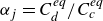 $\alpha _j=C^{eq}_d/C^{eq}_c$
, i.e. the ratio between the chemical species equilibrium concentration in the dispersed phase and in the carrier flow. Since our objective is to understand how the diffusivity of species influences the overall mass transfer, we keep all the parameters constant, but
$\alpha _j=C^{eq}_d/C^{eq}_c$
, i.e. the ratio between the chemical species equilibrium concentration in the dispersed phase and in the carrier flow. Since our objective is to understand how the diffusivity of species influences the overall mass transfer, we keep all the parameters constant, but ${\textit{Sc}}$
and
${\textit{Sc}}$
and $D_r$
. In particular, we assume
$D_r$
. In particular, we assume $\mu _r = 1$
,
$\mu _r = 1$
, $\rho _r = 1$
and
$\rho _r = 1$
and $\alpha _j=1$
. In addition, indicating with
$\alpha _j=1$
. In addition, indicating with $u_b$
the bulk velocity, and with the reference velocity and length scales given by
$u_b$
the bulk velocity, and with the reference velocity and length scales given by $\tilde {U}=2 u_b$
and
$\tilde {U}=2 u_b$
and $\tilde {L}= h$
, we obtain
$\tilde {L}= h$
, we obtain ${\textit{Re}}=10\,000$
and
${\textit{Re}}=10\,000$
and ${We}=3100$
. The corresponding values of the shear Reynolds and Weber numbers are
${We}=3100$
. The corresponding values of the shear Reynolds and Weber numbers are ${\textit{Re}}_{\tau } = u_{\tau } h / \nu \approx 300$
and
${\textit{Re}}_{\tau } = u_{\tau } h / \nu \approx 300$
and ${We}_{\tau } = \rho u_{\tau }^2 h / \sigma \approx 2.79$
, since
${We}_{\tau } = \rho u_{\tau }^2 h / \sigma \approx 2.79$
, since $ {\textit{Re}}_{\tau } \approx 0.09Re^{0.88}$
(Pope Reference Pope2001).
$ {\textit{Re}}_{\tau } \approx 0.09Re^{0.88}$
(Pope Reference Pope2001).
These values are representative of a physical situation characterised by a water and oil liquid–liquid mixture, with $\sigma \simeq 3 \times 10^{-3}\,{\rm N\,m}^{-1}$
, in a channel with characteristic velocity
$\sigma \simeq 3 \times 10^{-3}\,{\rm N\,m}^{-1}$
, in a channel with characteristic velocity $\tilde {U} \simeq 1\,{\rm m\,s}^{-1}$
and characteristic length
$\tilde {U} \simeq 1\,{\rm m\,s}^{-1}$
and characteristic length $h \simeq \mathcal{O}(10^{-2})$
m (see Than et al. Reference Than, Preziosi, Josephl and Arney1988). Regarding the choice of
$h \simeq \mathcal{O}(10^{-2})$
m (see Than et al. Reference Than, Preziosi, Josephl and Arney1988). Regarding the choice of ${\textit{Sc}}$
and
${\textit{Sc}}$
and $D_r$
, we analyse two different situations: (i) the Schmidt number of the carrier phase is varied from
$D_r$
, we analyse two different situations: (i) the Schmidt number of the carrier phase is varied from ${\textit{Sc}}_c=0.5$
to
${\textit{Sc}}_c=0.5$
to ${\textit{Sc}}_c=4$
, and is equal to the Schmidt number inside the dispersed phase, so that the diffusivity ratio is
${\textit{Sc}}_c=4$
, and is equal to the Schmidt number inside the dispersed phase, so that the diffusivity ratio is $D_r=1$
(case A); (ii) the Schmidt number of the carrier phase is varied from
$D_r=1$
(case A); (ii) the Schmidt number of the carrier phase is varied from ${\textit{Sc}}_c=0.5$
to
${\textit{Sc}}_c=0.5$
to ${\textit{Sc}}_c=4$
, while the Schmidt number inside the dispersed phase is kept constant,
${\textit{Sc}}_c=4$
, while the Schmidt number inside the dispersed phase is kept constant, ${\textit{Sc}}_d=0.01$
, so that the diffusivity ratio is systematically increased from 50 to 400 (case B). The complete list of simulations performed in the present study is given in table 1. The computational grid is uniform in the streamwise and spanwise directions, where the flow is periodic, while it is non-uniform in the wall-normal direction (no-slip condition), along which the natural grid stretching proposed by Pirozzoli & Orlandi (Reference Pirozzoli and Orlandi2021) is used to cluster computational points near the walls. In wall units (obtained using
${\textit{Sc}}_d=0.01$
, so that the diffusivity ratio is systematically increased from 50 to 400 (case B). The complete list of simulations performed in the present study is given in table 1. The computational grid is uniform in the streamwise and spanwise directions, where the flow is periodic, while it is non-uniform in the wall-normal direction (no-slip condition), along which the natural grid stretching proposed by Pirozzoli & Orlandi (Reference Pirozzoli and Orlandi2021) is used to cluster computational points near the walls. In wall units (obtained using $\nu /u_{\tau }$
as reference length), the grid resolution for each case is
$\nu /u_{\tau }$
as reference length), the grid resolution for each case is $\Delta x^+ = \Delta z^+ \approx 3.27$
, while
$\Delta x^+ = \Delta z^+ \approx 3.27$
, while $\Delta y^+$
ranges between
$\Delta y^+$
ranges between $0.046$
and
$0.046$
and $3.06$
, enough to solve the characteristic length scale of turbulence (the Kolmogorov scale,
$3.06$
, enough to solve the characteristic length scale of turbulence (the Kolmogorov scale, $\eta _k$
) (Bernardini, Pirozzoli & Orlandi Reference Bernardini, Pirozzoli and Orlandi2014). When a scalar is transported in a turbulent flow, a second characteristic length scale is present, the Batchelor scale,
$\eta _k$
) (Bernardini, Pirozzoli & Orlandi Reference Bernardini, Pirozzoli and Orlandi2014). When a scalar is transported in a turbulent flow, a second characteristic length scale is present, the Batchelor scale,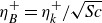 $\eta _B^+=\eta _k^+/\sqrt {\textit{Sc}}$
, with
$\eta _B^+=\eta _k^+/\sqrt {\textit{Sc}}$
, with ${\textit{Sc}}$
the Schmidt number (Batchelor Reference Batchelor1959). Naturally, when
${\textit{Sc}}$
the Schmidt number (Batchelor Reference Batchelor1959). Naturally, when ${\textit{Sc}}=4$
,
${\textit{Sc}}=4$
, $\eta _B^+=(1/2)\eta _k^+$
. In the context of our simulations, and specifically to tackle this aspect, the employed computational grid (with
$\eta _B^+=(1/2)\eta _k^+$
. In the context of our simulations, and specifically to tackle this aspect, the employed computational grid (with $\Delta x^+=\Delta z^+=3.27$
and
$\Delta x^+=\Delta z^+=3.27$
and $\Delta y^+\lt 3.06$
), which is over-refined for the flow field (i.e. to capture
$\Delta y^+\lt 3.06$
), which is over-refined for the flow field (i.e. to capture $\eta _k^+$
), is perfectly suitable also for the scalar. Further details of the grid sensitivity analysis are given in Appendix A.3.
$\eta _k^+$
), is perfectly suitable also for the scalar. Further details of the grid sensitivity analysis are given in Appendix A.3.
Overview of the main simulation parameters. We run two series of simulations: case A simulations, where the Schmidt number of the carrier phase is varied from ${\textit{Sc}}_c=0.5$
to
${\textit{Sc}}_c=0.5$
to ${\textit{Sc}}_c=4$
, and is equal to the Schmidt number inside the drops, so that the diffusivity ratio is
${\textit{Sc}}_c=4$
, and is equal to the Schmidt number inside the drops, so that the diffusivity ratio is $D_r=1$
; and case B simulations, where the Schmidt number of the carrier phase is varied from
$D_r=1$
; and case B simulations, where the Schmidt number of the carrier phase is varied from ${\textit{Sc}}_c=0.5$
to
${\textit{Sc}}_c=0.5$
to ${\textit{Sc}}_c=4$
, while the Schmidt number inside the dispersed phase is kept constant,
${\textit{Sc}}_c=4$
, while the Schmidt number inside the dispersed phase is kept constant, ${\textit{Sc}}_d=0.01$
(i.e.
${\textit{Sc}}_d=0.01$
(i.e. $D_r$
is increased from 50 to 400). The values of
$D_r$
is increased from 50 to 400). The values of ${\textit{Sc}}$
,
${\textit{Sc}}$
, $D_r$
and
$D_r$
and $\alpha _j$
are explicitly given. For all simulations,
$\alpha _j$
are explicitly given. For all simulations, $\mu _r = 1$
,
$\mu _r = 1$
, $\rho _r = 1$
.
$\rho _r = 1$
.

4. Results
Mass transfer in a drop-laden turbulent flow is a complex, hierarchical process. The building block of this process is represented by the dynamics of each drop: each drop interacts with local turbulence, which induces drop deformation and internal circulation; but at the same time each drop interacts with the other drops in a collective, large-scale, dynamics. This is visualised in figure 1, where a snapshot of the drop shape and location is given, together with a volume-rendering representation of the solute concentration (from yellow – high – to cyan – low – solute concentration). In an effort to clarify further the main ingredients of this dynamics, we focus on a single drop, immersed in turbulence, which comes closer to another drop. The situation is sketched in figure 2, via a sequence of snapshots representing two individual drops in the process of merging, for two different values of the molecular diffusivity inside the dispersed phase (case A2 and case B2 in table 1). We recall that the efficiency of the mass-transfer process crucially depends on the value of the molecular diffusivity of either fluid (here represented by its dimensionless counterpart, the Schmidt number, ${\textit{Sc}}$
). For case A2, shown in the top two rows of figure 2, the value of the Schmidt number outside and inside of the dispersed phase is the same and it is equal to
${\textit{Sc}}$
). For case A2, shown in the top two rows of figure 2, the value of the Schmidt number outside and inside of the dispersed phase is the same and it is equal to ${\textit{Sc}}_c={\textit{Sc}}_d=1.0$
. For case B2, shown in the bottom two rows of figure 2, the value of the Schmidt number outside of the drop is
${\textit{Sc}}_c={\textit{Sc}}_d=1.0$
. For case B2, shown in the bottom two rows of figure 2, the value of the Schmidt number outside of the drop is ${\textit{Sc}}_c=1.0$
while the value inside the drops is
${\textit{Sc}}_c=1.0$
while the value inside the drops is ${\textit{Sc}}_b=0.01$
(i.e. much larger diffusivity, typical of gases). We start by considering case A2. Two drops, one characterised by a higher species concentration (orange-to-yellow inner colour) and one by lower concentration (blue inner colour), merge. Because of the relatively low species diffusivity inside the drop (
${\textit{Sc}}_b=0.01$
(i.e. much larger diffusivity, typical of gases). We start by considering case A2. Two drops, one characterised by a higher species concentration (orange-to-yellow inner colour) and one by lower concentration (blue inner colour), merge. Because of the relatively low species diffusivity inside the drop ( ${\textit{Sc}}_d=1.0$
), species transport from the very beginning (
${\textit{Sc}}_d=1.0$
), species transport from the very beginning ( $t^+=295$
) is mainly due to advection. When the two drops merge, the species transport is still dominated by advection, and the mixing inside the newly formed drop is not very efficient (due to the relatively small characteristic size of the drop), and the resulting species concentration is inhomogeneous and characterised by larger gradients and fluctuations (see snapshots between
$t^+=295$
) is mainly due to advection. When the two drops merge, the species transport is still dominated by advection, and the mixing inside the newly formed drop is not very efficient (due to the relatively small characteristic size of the drop), and the resulting species concentration is inhomogeneous and characterised by larger gradients and fluctuations (see snapshots between $t^+=310$
and
$t^+=310$
and $t^+=375$
). We now move to case B2, in which the species diffusivity inside the drop is much larger than outside the drop (
$t^+=375$
). We now move to case B2, in which the species diffusivity inside the drop is much larger than outside the drop ( ${\textit{Sc}}_d=0.01$
,
${\textit{Sc}}_d=0.01$
, ${\textit{Sc}}_c=1.0$
). At the beginning, the two drops are characterised by a different concentration (see the different colours inside the drops, one close to dark blue, the other close to light blue at
${\textit{Sc}}_c=1.0$
). At the beginning, the two drops are characterised by a different concentration (see the different colours inside the drops, one close to dark blue, the other close to light blue at $t^+=295$
). However, and differently from the previous case, the species concentration inside each of the two drops is much more homogeneous. Once the drops have merged, the internal concentrations rapidly homogenise by diffusion (which is the leading transport mechanism in this case, since the time scale of diffusion is much shorter than that of advection) and the concentration gradients inside the newly formed drop are smaller.
$t^+=295$
). However, and differently from the previous case, the species concentration inside each of the two drops is much more homogeneous. Once the drops have merged, the internal concentrations rapidly homogenise by diffusion (which is the leading transport mechanism in this case, since the time scale of diffusion is much shorter than that of advection) and the concentration gradients inside the newly formed drop are smaller.
Three-dimensional rendering of mass transport in a drop-laden turbulent channel flow. The colour scale represents species concentration: yellow indicates high concentration, while blue indicates low concentration. The flow, driven by a pressure gradient, moves from left to right. The inset shows a cross-section of a drop, illustrating the internal distribution of species concentration. Results correspond to case B2, with ${\textit{Sc}}= 1$
,
${\textit{Sc}}= 1$
, $D_r=100$
.
$D_r=100$
.

Snapshots separated by $\Delta t^+ = 5$
of a solute concentration field on a horizontal plane
$\Delta t^+ = 5$
of a solute concentration field on a horizontal plane $(x{-}z)$
at time sequence
$(x{-}z)$
at time sequence $t^+= ( 295 ,375)$
. Influence of the coalescence event on the concentration field inside and outside of the drop for case A2 with Schmidt number of the dispersed phase
$t^+= ( 295 ,375)$
. Influence of the coalescence event on the concentration field inside and outside of the drop for case A2 with Schmidt number of the dispersed phase ${\textit{Sc}}_d=1.0$
(without diffusivity ratio) and case B2 with
${\textit{Sc}}_d=1.0$
(without diffusivity ratio) and case B2 with ${\textit{Sc}}_d=0.01$
(with diffusivity ratio). Both simulations are characterised by a Schmidt number in the carrier flow
${\textit{Sc}}_d=0.01$
(with diffusivity ratio). Both simulations are characterised by a Schmidt number in the carrier flow ${\textit{Sc}}_c=1.0$
.
${\textit{Sc}}_c=1.0$
.

Instantaneous visualisation of the solute concentration field on a portion of a horizontal plane ( $x{-}z$
) of length
$x{-}z$
) of length $\Delta L_x /h = 6.08$
and width
$\Delta L_x /h = 6.08$
and width $\Delta L_z /h = 4.28$
, located at
$\Delta L_z /h = 4.28$
, located at $y/h=0.5$
at
$y/h=0.5$
at $t^+=500$
. The interface of the drops (iso-level
$t^+=500$
. The interface of the drops (iso-level $\chi =0.5$
) is represented by the white line. Each row refers to a different Schmidt number of the carrier phase: from top to bottom,
$\chi =0.5$
) is represented by the white line. Each row refers to a different Schmidt number of the carrier phase: from top to bottom, ${\textit{Sc}}_c =0.5,\ 1.0,\ 2.0,\ 4.0$
, respectively. (a) Case A. (b) Case B.
${\textit{Sc}}_c =0.5,\ 1.0,\ 2.0,\ 4.0$
, respectively. (a) Case A. (b) Case B.

Also visible is the fact that the overall efficiency of the species transport mechanism strongly depends on the species diffusivity in the carrier flow ( ${\textit{Sc}}_c$
) where the drops are immersed: indeed, the bottleneck of the mass-transfer process is represented by the Schmidt number of the carrier flow, with the Schmidt number of the drops playing a relatively less significant – though important – role, as discussed below. This is clearly visualised in figure 3, where the instantaneous distribution (taken at
${\textit{Sc}}_c$
) where the drops are immersed: indeed, the bottleneck of the mass-transfer process is represented by the Schmidt number of the carrier flow, with the Schmidt number of the drops playing a relatively less significant – though important – role, as discussed below. This is clearly visualised in figure 3, where the instantaneous distribution (taken at $t^+=500$
) of the species concentration on a portion of a horizontal plane (
$t^+=500$
) of the species concentration on a portion of a horizontal plane ( $x{-}z$
) of length
$x{-}z$
) of length $\Delta L_x /h = 6.08$
and width
$\Delta L_x /h = 6.08$
and width $\Delta L_z /h = 4.28$
, located at
$\Delta L_z /h = 4.28$
, located at $y/h=0.5$
(i.e. where drops are initially released), is given for all cases considered in the present study. Each row corresponds to a different Schmidt number of the carrier flow, from
$y/h=0.5$
(i.e. where drops are initially released), is given for all cases considered in the present study. Each row corresponds to a different Schmidt number of the carrier flow, from ${\textit{Sc}}_c=0.5$
(top) to
${\textit{Sc}}_c=0.5$
(top) to ${\textit{Sc}}_c=4$
(bottom). The left-hand column refers to simulations in which the Schmidt number of the dispersed phase is equal to the Schmidt number of the carrier flow,
${\textit{Sc}}_c=4$
(bottom). The left-hand column refers to simulations in which the Schmidt number of the dispersed phase is equal to the Schmidt number of the carrier flow, ${\textit{Sc}}_d={\textit{Sc}}_c$
(simulations A in table 1); the right-hand column refers to simulations in which the Schmidt number of the dispersed phase is kept constant
${\textit{Sc}}_d={\textit{Sc}}_c$
(simulations A in table 1); the right-hand column refers to simulations in which the Schmidt number of the dispersed phase is kept constant ${\textit{Sc}}_d=0.01$
, i.e. large diffusivity inside the drops (simulations B in table 1). As expected, the smaller is
${\textit{Sc}}_d=0.01$
, i.e. large diffusivity inside the drops (simulations B in table 1). As expected, the smaller is ${\textit{Sc}}_c$
(i.e. the larger the species diffusivity), the faster is the mass transfer from the dispersed phase to the carrier flow (see the difference between the concentration inside the drops at
${\textit{Sc}}_c$
(i.e. the larger the species diffusivity), the faster is the mass transfer from the dispersed phase to the carrier flow (see the difference between the concentration inside the drops at ${\textit{Sc}}_c=0.5$
– close to blue, top row – and the solute concentration inside the drop at
${\textit{Sc}}_c=0.5$
– close to blue, top row – and the solute concentration inside the drop at ${\textit{Sc}}_c=4$
– close to red/yellow, bottom row). In addition, while at
${\textit{Sc}}_c=4$
– close to red/yellow, bottom row). In addition, while at ${\textit{Sc}}_c=0.5$
the species concentration in the carrier flow is more homogeneous (because the species diffuses more efficiently), at higher
${\textit{Sc}}_c=0.5$
the species concentration in the carrier flow is more homogeneous (because the species diffuses more efficiently), at higher ${\textit{Sc}}_c$
the species concentration is characterised by sharper gradients and thinner filamentary structures. However, and because of the non-negligible role of the species diffusivity inside the drops, even when the Schmidt number of the carrier phase is the same between two cases (comparison of cases arranged in each row), the species concentration in the carrier phase can be slightly different. This is due to the fact that the concentration inside the drops can change (different
${\textit{Sc}}_c$
the species concentration is characterised by sharper gradients and thinner filamentary structures. However, and because of the non-negligible role of the species diffusivity inside the drops, even when the Schmidt number of the carrier phase is the same between two cases (comparison of cases arranged in each row), the species concentration in the carrier phase can be slightly different. This is due to the fact that the concentration inside the drops can change (different ${\textit{Sc}}_d$
), and so does the concentration at the interface, thereby inducing a different interfacial flux of species and a different concentration in the carrier flow. We will come back to this point later, when we compare the average mass-transfer flux for cases at the same
${\textit{Sc}}_d$
), and so does the concentration at the interface, thereby inducing a different interfacial flux of species and a different concentration in the carrier flow. We will come back to this point later, when we compare the average mass-transfer flux for cases at the same ${\textit{Sc}}_c$
but different
${\textit{Sc}}_c$
but different ${\textit{Sc}}_d$
(see figure 5 and corresponding discussion).
${\textit{Sc}}_d$
(see figure 5 and corresponding discussion).
4.1. Quantitative analysis
We now characterise the mass-transfer process from a quantitative viewpoint. To begin with, we focus on the average solute concentration in the dispersed phase, $\bar {c}_d$
, and in the carrier flow,
$\bar {c}_d$
, and in the carrier flow, $\bar {c}_c$
, computed as
$\bar {c}_c$
, computed as
 \begin{equation} \bar {c}_d = \frac {1}{V_d} \int _{V_d} c \mathrm{d} V, \quad \bar {c}_c = \frac {1}{V_c} \int _{V_c} c \mathrm{d} V, \end{equation}
where $V_d$
and
$V_d$
and $V_c$
are the volume of all drops (considered as an ensemble) and of the carrier flow, respectively. The time evolution of
$V_c$
are the volume of all drops (considered as an ensemble) and of the carrier flow, respectively. The time evolution of $\bar {c}_d$
and
$\bar {c}_d$
and $\bar {c}_c$
is shown by symbols, for all different simulations performed in the present study, in figure 4. In particular, figure 4(a) refers to case A simulations (i.e.
$\bar {c}_c$
is shown by symbols, for all different simulations performed in the present study, in figure 4. In particular, figure 4(a) refers to case A simulations (i.e. ${\textit{Sc}}_c=S_d$
increasing from 0.5 to 4, and keeping diffusivity ratio
${\textit{Sc}}_c=S_d$
increasing from 0.5 to 4, and keeping diffusivity ratio $D_r=1$
), while figure 4(b) refers to case B simulations (i.e.
$D_r=1$
), while figure 4(b) refers to case B simulations (i.e. ${\textit{Sc}}_c$
increasing from 0.5 to 4 while
${\textit{Sc}}_c$
increasing from 0.5 to 4 while ${\textit{Sc}}_d=0.01$
, which gives a diffusivity ratio
${\textit{Sc}}_d=0.01$
, which gives a diffusivity ratio $D_r$
increasing from 50 to 400). Together with the results given by the DNS (symbols), we also provide the prediction obtained by a simplified lumped-parameter model (solid lines), whose detailed description is given in § 5. Starting from the initial condition, at which the species concentration inside the drops is
$D_r$
increasing from 50 to 400). Together with the results given by the DNS (symbols), we also provide the prediction obtained by a simplified lumped-parameter model (solid lines), whose detailed description is given in § 5. Starting from the initial condition, at which the species concentration inside the drops is $\bar {c}_d=1$
– i.e. fully saturated drops – and
$\bar {c}_d=1$
– i.e. fully saturated drops – and $\bar {c}_c=0$
– i.e. carrier flow depleted of species – and regardless of the value of the species diffusivity in both phases (i.e.
$\bar {c}_c=0$
– i.e. carrier flow depleted of species – and regardless of the value of the species diffusivity in both phases (i.e. ${\textit{Sc}}$
),
${\textit{Sc}}$
), $\bar {c}_d$
monotonically decreases and
$\bar {c}_d$
monotonically decreases and $\bar {c}_c$
monotonically increases, until the equilibrium steady-state condition
$\bar {c}_c$
monotonically increases, until the equilibrium steady-state condition $\bar {c}_{\textit{ss}} = \bar {c}_d=\bar {c}_c = 0.054$
is reached. During this transient, mass transfer is progressively reduced until it finally stops. For this reason, we decided to block our simulations at
$\bar {c}_{\textit{ss}} = \bar {c}_d=\bar {c}_c = 0.054$
is reached. During this transient, mass transfer is progressively reduced until it finally stops. For this reason, we decided to block our simulations at $t^+=3000$
, a condition at which
$t^+=3000$
, a condition at which $(\bar {c}_{\textit{ss}} - \bar {c}_c)/\bar {c}_{\textit{ss}} \lt 2 \%$
, for all cases. The influence of the Schmidt number of the carrier flow,
$(\bar {c}_{\textit{ss}} - \bar {c}_c)/\bar {c}_{\textit{ss}} \lt 2 \%$
, for all cases. The influence of the Schmidt number of the carrier flow, ${\textit{Sc}}_c$
, is apparent: the smaller the value of
${\textit{Sc}}_c$
, is apparent: the smaller the value of ${\textit{Sc}}_c$
(i.e. the larger the species diffusivity in the carrier flow), the faster the mass-transfer process, no matter the value of
${\textit{Sc}}_c$
(i.e. the larger the species diffusivity in the carrier flow), the faster the mass-transfer process, no matter the value of ${\textit{Sc}}_d$
(i.e. similar trends are observed for case A and case B simulations).
${\textit{Sc}}_d$
(i.e. similar trends are observed for case A and case B simulations).
Time evolution of the average species concentration in the drops and in the carrier phase for (a) case A (without diffusivity ratio) and (b) case B (with diffusivity ratio) simulations, at Schmidt number of the carrier flow ${\textit{Sc}}_c = 0.5,\ 1,\ 2,\ 4$
. Symbols (filled squares) represent results obtained by DNS, while solid lines represent the predictions obtained by the simplified phenomenological model, (5.12), described in § 5.
${\textit{Sc}}_c = 0.5,\ 1,\ 2,\ 4$
. Symbols (filled squares) represent results obtained by DNS, while solid lines represent the predictions obtained by the simplified phenomenological model, (5.12), described in § 5.

Of interest is now to evaluate the evolution of the mass-transfer process considering the same Schmidt number in the carrier flow, but a different Schmidt number in the dispersed phase (i.e comparing one case A with one case B simulation). This comparison cannot be easily done by looking at figure 4, where case A and case B simulations are shown in different panels. Therefore, we decided to make a one-to-one comparison, focusing on the case ${\textit{Sc}}_c=1$
and plotting simulation A2 (
${\textit{Sc}}_c=1$
and plotting simulation A2 ( ${\textit{Sc}}_d={\textit{Sc}}_c=1$
, i.e.
${\textit{Sc}}_d={\textit{Sc}}_c=1$
, i.e. $D_r=1$
) together with simulation B2 (
$D_r=1$
) together with simulation B2 ( ${\textit{Sc}}_d=0.01$
,
${\textit{Sc}}_d=0.01$
, ${\textit{Sc}}_c=1$
, i.e.
${\textit{Sc}}_c=1$
, i.e. $D_r=100$
). Results are shown in figure 5 by plotting the derivative in time of the average drop concentration,
$D_r=100$
). Results are shown in figure 5 by plotting the derivative in time of the average drop concentration, $\mathrm{d} \bar {c}_d/\mathrm{d} t$
(main panel) as well as the average concentration,
$\mathrm{d} \bar {c}_d/\mathrm{d} t$
(main panel) as well as the average concentration, $c_d$
and
$c_d$
and $c_c$
(inset). At the beginning, the species is released more efficiently for case B (higher
$c_c$
(inset). At the beginning, the species is released more efficiently for case B (higher $\mathrm{d}\bar {c}_d/\mathrm{d} t$
, main panel of figure 5
a) than for case A. This result, which is expected given the larger species diffusivity for case B (
$\mathrm{d}\bar {c}_d/\mathrm{d} t$
, main panel of figure 5
a) than for case A. This result, which is expected given the larger species diffusivity for case B ( ${\textit{Sc}}_d=0.01$
), reflects onto a corresponding decrease of
${\textit{Sc}}_d=0.01$
), reflects onto a corresponding decrease of $c_d$
that is faster for case B than for case A (inset of figure 5
a). There is a crossover point between
$c_d$
that is faster for case B than for case A (inset of figure 5
a). There is a crossover point between $\mathrm{d} \bar {c}_d / \mathrm{d} t$
for case A2 and B2, after which
$\mathrm{d} \bar {c}_d / \mathrm{d} t$
for case A2 and B2, after which $\mathrm{d} \bar {c}_d / \mathrm{d} t$
for case A2 becomes greater than
$\mathrm{d} \bar {c}_d / \mathrm{d} t$
for case A2 becomes greater than $\mathrm{d} \bar {c}_d / \mathrm{d} t$
for case B2, indicating that mass transfer becomes more efficient for case A2 than for case B2.
$\mathrm{d} \bar {c}_d / \mathrm{d} t$
for case B2, indicating that mass transfer becomes more efficient for case A2 than for case B2.
This is investigated by taking three snapshots – one before the crossover, at $t^+=25$
(figure 5
b), one at the crossover, at
$t^+=25$
(figure 5
b), one at the crossover, at $t^+=150$
(figure 5
c), and one after the crossover, at
$t^+=150$
(figure 5
c), and one after the crossover, at $t^+=600$
(figure 5
d) – of the solute concentration on a plane parallel to the wall and located at
$t^+=600$
(figure 5
d) – of the solute concentration on a plane parallel to the wall and located at $z=h/2$
(plane at which drops are initially released). At the beginning the species concentration is rather uniform for both cases A2 and B2 (see figure 5
b), and the mass-transfer rate is controlled by the diffusivity inside the drop, giving higher mass-transfer rates (flux of species) for case B2, and therefore lower species concentration inside the drops (see bullet points at
$z=h/2$
(plane at which drops are initially released). At the beginning the species concentration is rather uniform for both cases A2 and B2 (see figure 5
b), and the mass-transfer rate is controlled by the diffusivity inside the drop, giving higher mass-transfer rates (flux of species) for case B2, and therefore lower species concentration inside the drops (see bullet points at $t^+=150$
in figure 5
a). At later stages, the situation is reversed. Mass transfer (flux of species) becomes more efficient for case A, given the relatively larger average species concentration inside the drops.
$t^+=150$
in figure 5
a). At later stages, the situation is reversed. Mass transfer (flux of species) becomes more efficient for case A, given the relatively larger average species concentration inside the drops.
While case B (with diffusivity ratio $D_r=100$
) exhibits a faster species flux than case A only during the early stages of the process, the overall process reaches a steady-state condition more rapidly (inset of figure 5
a). This indicates that an increase of the species diffusivity inside the drop (case B,
$D_r=100$
) exhibits a faster species flux than case A only during the early stages of the process, the overall process reaches a steady-state condition more rapidly (inset of figure 5
a). This indicates that an increase of the species diffusivity inside the drop (case B, $D_r\gt 1$
) enhances the overall mass-transfer efficiency, thereby resulting in a larger mass-transfer velocity compared with a case with unitary diffusivity ratio (case A,
$D_r\gt 1$
) enhances the overall mass-transfer efficiency, thereby resulting in a larger mass-transfer velocity compared with a case with unitary diffusivity ratio (case A, $D_r=1$
).
$D_r=1$
).
(a) Time evolution of the flux of species $\mathrm{d} \overline {c}_d/ \mathrm{d} t$
for case A at
$\mathrm{d} \overline {c}_d/ \mathrm{d} t$
for case A at $D_r=1$
and case B at
$D_r=1$
and case B at $D_r=100$
and Schmidt number of carrier phase
$D_r=100$
and Schmidt number of carrier phase ${\textit{Sc}}_c=1$
. In the inset, the behaviour of the average solute concentration in dispersed phase and carrier flow,
${\textit{Sc}}_c=1$
. In the inset, the behaviour of the average solute concentration in dispersed phase and carrier flow, $\overline {c}_d,\overline {c}_c$
, is shown as a function of time. (b–d) Instantaneous visualisation of the solute concentration field on a horizontal plane (x–z) located at the channel quarter for
$\overline {c}_d,\overline {c}_c$
, is shown as a function of time. (b–d) Instantaneous visualisation of the solute concentration field on a horizontal plane (x–z) located at the channel quarter for $t^+ =25,\ 150,\ 600$
.
$t^+ =25,\ 150,\ 600$
.

5. A lumped-parameter model for mass transport in drop-laden flows
The average concentration profiles shown in figure 4 exhibit clear self-similarity. This behaviour can be captured using a simplified phenomenological model for mass transfer in drop-laden turbulent channel flow. Consistent with the assumptions adopted in the DNS, the lumped-parameter model considers identical density and viscosity for the dispersed and carrier phases ( $\rho _r = 1$
,
$\rho _r = 1$
, $\mu _r = 1$
) (Mangani et al. Reference Mangani, Roccon, Zonta and Soldati2024).
$\mu _r = 1$
) (Mangani et al. Reference Mangani, Roccon, Zonta and Soldati2024).
We begin by considering the mass transfer from a drop of diameter $d_d^*$
to the surrounding fluid:
$d_d^*$
to the surrounding fluid:
 \begin{equation} \frac {\mathrm{d} N^*}{\mathrm{d} t^*} = \mathcal{K}^* A_d^* \left ( c_d^* - c_c^* \right )\! , \end{equation}
where $N^*$
is the number of moles of a given species,
$N^*$
is the number of moles of a given species, $A_d^*$
is the external surface of the drop,
$A_d^*$
is the external surface of the drop, $\mathcal{K}^*$
is the mass transfer coefficient, while
$\mathcal{K}^*$
is the mass transfer coefficient, while $c_d^*$
and
$c_d^*$
and $c_c^*$
are the concentrations of the species inside the dispersed phase and in the carrier flow. Note that the asterisk denotes dimensional quantities. In analogy with heat-transfer processes, the mass-transfer coefficient can be estimated as the ratio between the diffusion coefficient (of the carrier flow),
$c_c^*$
are the concentrations of the species inside the dispersed phase and in the carrier flow. Note that the asterisk denotes dimensional quantities. In analogy with heat-transfer processes, the mass-transfer coefficient can be estimated as the ratio between the diffusion coefficient (of the carrier flow), $D^*$
, and a reference length scale, here represented by the concentration boundary-layer thickness
$D^*$
, and a reference length scale, here represented by the concentration boundary-layer thickness $\delta _c^*$
:
$\delta _c^*$
:
 \begin{equation} \mathcal{K}^* \sim D^* / \delta _c^* . \end{equation}
In addition, the concentration boundary layer $\delta _c^*$
is expressed as
$\delta _c^*$
is expressed as $\delta _c^* = \delta ^* Sc^{-\beta }$
, where
$\delta _c^* = \delta ^* Sc^{-\beta }$
, where $\delta ^*$
is the momentum boundary-layer thickness and
$\delta ^*$
is the momentum boundary-layer thickness and $\beta$
is an exponent that depends on the flow conditions in the near-interface region. Typical values range from
$\beta$
is an exponent that depends on the flow conditions in the near-interface region. Typical values range from $\beta = 1/3$
for no-slip conditions to
$\beta = 1/3$
for no-slip conditions to $\beta = 1/2$
, commonly assumed for clean drops or bubbles. In the present study,
$\beta = 1/2$
, commonly assumed for clean drops or bubbles. In the present study, $\beta = 1/2$
is adopted (see Mangani et al. Reference Mangani, Roccon, Zonta and Soldati2024).
$\beta = 1/2$
is adopted (see Mangani et al. Reference Mangani, Roccon, Zonta and Soldati2024).
With these assumptions, recalling that the concentration of species is $c^*=N^*/V^*_d$
, with
$c^*=N^*/V^*_d$
, with $V^*_d$
the drop volume, and using the initial drop-to-carrier concentration difference
$V^*_d$
the drop volume, and using the initial drop-to-carrier concentration difference $\Delta c^{*,0} = c^{*,0}_{d} - c^{*,0}_{c}$
as the reference concentration (superscript ‘0’ denotes the initial time),
$\Delta c^{*,0} = c^{*,0}_{d} - c^{*,0}_{c}$
as the reference concentration (superscript ‘0’ denotes the initial time), $h^*/u_b^*$
as the reference time and
$h^*/u_b^*$
as the reference time and $h^*$
as the reference length, (5.1) can be rewritten in dimensionless form as follows:
$h^*$
as the reference length, (5.1) can be rewritten in dimensionless form as follows:
 \begin{equation} \frac {\mathrm{d} c_d}{\mathrm{d} t}= 6 {\textit{Re}}_{\delta }^{-1} Sc ^{-1+\beta } \left ( {d_d} \right )^{-1} \left ( c_d - c_c \right )\! , \end{equation}
where $d_d$
is the dimensionless drop diameter in outer units, while
$d_d$
is the dimensionless drop diameter in outer units, while ${\textit{Re}}_{\delta }=u_{b}^* \delta ^* /\nu ^*$
is the Reynolds number based on the boundary-layer thickness (which can be assumed constant among the different cases, since the concentration is here a passive scalar). In the present case, since
${\textit{Re}}_{\delta }=u_{b}^* \delta ^* /\nu ^*$
is the Reynolds number based on the boundary-layer thickness (which can be assumed constant among the different cases, since the concentration is here a passive scalar). In the present case, since $\beta =1/2$
(typical of clean drops/bubbles), we obtain
$\beta =1/2$
(typical of clean drops/bubbles), we obtain
 \begin{equation} \frac {\mathrm{d} c_d}{\mathrm{d} t}= \mathcal{C} Sc ^{-1/2} \left ( {d_d} \right )^{-1} \left ( c_d - c_c \right )\! , \end{equation}
where the model parameter $\mathcal{C}=6 {\textit{Re}}_{\delta }^{-1}=6 \times 10^{-3}$
is evaluated upon comparison of the model results with the current DNS data for the base case of
$\mathcal{C}=6 {\textit{Re}}_{\delta }^{-1}=6 \times 10^{-3}$
is evaluated upon comparison of the model results with the current DNS data for the base case of ${\textit{Sc}}_c=1$
and
${\textit{Sc}}_c=1$
and $D_r=1$
(simulation A2), and then kept for all simulations. It is worth mentioning that
$D_r=1$
(simulation A2), and then kept for all simulations. It is worth mentioning that $\mathcal{C}$
could change depending on the flow Reynolds number and/or the flow configuration. Now we extend the model considering that the concentration in the interior of the drop is not always uniform (as it would be in the case of perfectly mixed substances). If a concentration boundary layer exists also inside the drop, the mass-transfer process can be regarded as a two-step process: the mass transfer from the core of the drop to its interface (inner region labelled ‘i’, characterised by an inner mass-transfer coefficient,
$\mathcal{C}$
could change depending on the flow Reynolds number and/or the flow configuration. Now we extend the model considering that the concentration in the interior of the drop is not always uniform (as it would be in the case of perfectly mixed substances). If a concentration boundary layer exists also inside the drop, the mass-transfer process can be regarded as a two-step process: the mass transfer from the core of the drop to its interface (inner region labelled ‘i’, characterised by an inner mass-transfer coefficient, $\mathcal{K}^*_i$
); and the mass transfer from the interface to the surrounding fluid (outer region labelled ‘o’, characterised by an outer mass-transfer coefficient,
$\mathcal{K}^*_i$
); and the mass transfer from the interface to the surrounding fluid (outer region labelled ‘o’, characterised by an outer mass-transfer coefficient, $\mathcal{K}^*_o$
). With the constraint of the continuity of the molar flux at the interface,
$\mathcal{K}^*_o$
). With the constraint of the continuity of the molar flux at the interface,
 \begin{equation} \mathcal{K}_i^* A_d^* \left ( c_{d}^* - c_{d,i}^* \right ) = \mathcal{K}_o^* A_d^* \left ( c_{d,o}^* - c_c^* \right )\! , \end{equation}
recalling that $\mathcal{K}^*_o \propto D^*_o/\delta ^*_o$
and
$\mathcal{K}^*_o \propto D^*_o/\delta ^*_o$
and $\mathcal{K}^*_i \propto D^*_i/\delta ^*_i$
, and assuming that the kinematic viscosity is uniform,
$\mathcal{K}^*_i \propto D^*_i/\delta ^*_i$
, and assuming that the kinematic viscosity is uniform, $\nu ^*_i=\nu ^*_o=\nu ^*$
, and that the boundary-layer thickness inside and outside of the drop does not change,
$\nu ^*_i=\nu ^*_o=\nu ^*$
, and that the boundary-layer thickness inside and outside of the drop does not change, $\delta _o=\delta _i$
, we finally get
$\delta _o=\delta _i$
, we finally get
 \begin{equation} c_{d,i} =\frac {c_d {\textit{Sc}}_o+ c_c {\textit{Sc}}_i }{\alpha {\textit{Sc}}_i+{\textit{Sc}}_o} \, , \end{equation}
where ${\textit{Sc}}_i$
and
${\textit{Sc}}_i$
and ${\textit{Sc}}_o$
are the values of the Schmidt number inside and outside of the drop. Unlike the heat-transfer case, for mass transfer there can be a jump of concentration at the drop interface,
${\textit{Sc}}_o$
are the values of the Schmidt number inside and outside of the drop. Unlike the heat-transfer case, for mass transfer there can be a jump of concentration at the drop interface, $c_{d,o}=\alpha c_{d,i}$
, therefore giving
$c_{d,o}=\alpha c_{d,i}$
, therefore giving
 \begin{equation} \frac {\mathrm{d} c_d}{\mathrm{d} t}= \mathcal{C} {\textit{Sc}}_o ^{-1/2} \left ( {d_d} \right )^{-1} \left ( c_{d,o} - c_c \right )= \mathcal{C} {\textit{Sc}}_o ^{-1/2} \left ( {d_d} \right )^{-1} \left ( \alpha c_{d,i} - c_c \right )\! , \end{equation}
with $c_{d,i}$
given by (5.6). Note that in the present study we always have
$c_{d,i}$
given by (5.6). Note that in the present study we always have $\alpha =1$
, i.e. continuity of the concentration at the drop interface. Considering now that the turbulent flow is laden with drops of different diameters, the equation that describes the mass transfer from the
$\alpha =1$
, i.e. continuity of the concentration at the drop interface. Considering now that the turbulent flow is laden with drops of different diameters, the equation that describes the mass transfer from the $j$
th drop of given diameter
$j$
th drop of given diameter $d_{d,k}$
(with
$d_{d,k}$
(with $k$
indicating the
$k$
indicating the $k$
th diameter) becomes
$k$
th diameter) becomes
 \begin{equation} \frac {\mathrm{d} c_{d,j}}{\mathrm{d} t} = \mathcal{C} {\textit{Sc}}_o ^{-1/2} \left ( {d_{d,k}} \right )^{-1} \left ( c_{d,i,j} - c_c \right )\,=\mathcal{F}_j\, , \end{equation}
Steady-state size distribution of the drops. The Kolmogorov–Hinze scale is shown as the shaded area, computed using the values of the turbulent kinetic energy dissipation rate $\epsilon$
at
$\epsilon$
at $y/h = 0.5$
and
$y/h = 0.5$
and $y/h = 1$
. The reference Kolmogorov–Hinze scale, corresponding to the midpoint between these two limits, is indicated by the vertical dashed line. The two scaling laws,
$y/h = 1$
. The reference Kolmogorov–Hinze scale, corresponding to the midpoint between these two limits, is indicated by the vertical dashed line. The two scaling laws, $(d_{eq}/h)^{-3/2}$
for the coalescence-dominated regime (small drops) and
$(d_{eq}/h)^{-3/2}$
for the coalescence-dominated regime (small drops) and $(d_{eq}/h)^{-10/3}$
for the breakage-dominated regime (larger drops), are represented by the dash-dotted lines. In addition, datasets from several available literature studies are also reported: experimental wave breaking (Deane & Stokes Reference Deane and Stokes2002), numerical wave breaking (Di Giorgio et al. Reference Di Giorgio, Pirozzoli and Iafrati2022, Reference Di Giorgio, Pirozzoli and Iafrati2025), numerical homogeneous isotropic turbulence (Crialesi-Esposito, Chibbaro & Brandt Reference Crialesi-Esposito, Chibbaro and Brandt2023), numerical horizontal drop-laden channel (Mangani et al. Reference Mangani, Roccon, Zonta and Soldati2024; Procacci et al. Reference Procacci, Roccon, Solsvik and Soldati2025) and vertical bubble-laden channel (Procacci et al. Reference Procacci, Arosemena, Di Giorgio and Solsvik2026).
$(d_{eq}/h)^{-10/3}$
for the breakage-dominated regime (larger drops), are represented by the dash-dotted lines. In addition, datasets from several available literature studies are also reported: experimental wave breaking (Deane & Stokes Reference Deane and Stokes2002), numerical wave breaking (Di Giorgio et al. Reference Di Giorgio, Pirozzoli and Iafrati2022, Reference Di Giorgio, Pirozzoli and Iafrati2025), numerical homogeneous isotropic turbulence (Crialesi-Esposito, Chibbaro & Brandt Reference Crialesi-Esposito, Chibbaro and Brandt2023), numerical horizontal drop-laden channel (Mangani et al. Reference Mangani, Roccon, Zonta and Soldati2024; Procacci et al. Reference Procacci, Roccon, Solsvik and Soldati2025) and vertical bubble-laden channel (Procacci et al. Reference Procacci, Arosemena, Di Giorgio and Solsvik2026).

where $\mathcal{F}_j$
is a lumped-parameter representation of the rate of change of concentration for the
$\mathcal{F}_j$
is a lumped-parameter representation of the rate of change of concentration for the $j$
th drop. To make the model self-contained, we assume that the distribution of drops follows a predefined equilibrium size distribution (DSD), in which the number density of drops scales as
$j$
th drop. To make the model self-contained, we assume that the distribution of drops follows a predefined equilibrium size distribution (DSD), in which the number density of drops scales as ${d_d}^{-3/2}$
in the sub-Hinze-scale range, and as
${d_d}^{-3/2}$
in the sub-Hinze-scale range, and as ${d_d}^{-10/3}$
in the super-Hinze-scale range. The value of the Hinze scale,
${d_d}^{-10/3}$
in the super-Hinze-scale range. The value of the Hinze scale, $d_{H}=0.725 (\rho /\sigma )^{-3/5} \lvert \epsilon \lvert ^{-2/5}$
, with
$d_{H}=0.725 (\rho /\sigma )^{-3/5} \lvert \epsilon \lvert ^{-2/5}$
, with $\epsilon$
the turbulent kinetic energy dissipation, is expected to vary in the range
$\epsilon$
the turbulent kinetic energy dissipation, is expected to vary in the range $0.21\lt d_{H} \lt 0.41$
(see shaded area in figure 6), and corresponding to
$0.21\lt d_{H} \lt 0.41$
(see shaded area in figure 6), and corresponding to $\epsilon$
evaluated at
$\epsilon$
evaluated at $y/h=1/2$
, where the drops are initially released, or at the channel centre,
$y/h=1/2$
, where the drops are initially released, or at the channel centre, $y/h=1$
, where drops preferentially migrate. This type of distribution has been observed in the literature (Deane & Stokes Reference Deane and Stokes2002; Roccon et al. Reference Roccon, Zonta and Soldati2023), and is also confirmed in this study (see figure 6). To approximate the distribution shown in figure 6, we use 12 classes of drop diameter in the sub-Hinze range (
$y/h=1$
, where drops preferentially migrate. This type of distribution has been observed in the literature (Deane & Stokes Reference Deane and Stokes2002; Roccon et al. Reference Roccon, Zonta and Soldati2023), and is also confirmed in this study (see figure 6). To approximate the distribution shown in figure 6, we use 12 classes of drop diameter in the sub-Hinze range ( $0.035\lt d/h\lt 0.35$
), and 4 classes in the super-Hinze range (
$0.035\lt d/h\lt 0.35$
), and 4 classes in the super-Hinze range ( $0.35\lt d/h\lt 0.6$
). The choice of the minimum drop size, the maximum drop size and the Hinze drop size depends on the application, and should be evaluated according to experiments, DNS (as done in the present case) or other literature data/predictions. Equation (5.8) can be integrated in time to give
$0.35\lt d/h\lt 0.6$
). The choice of the minimum drop size, the maximum drop size and the Hinze drop size depends on the application, and should be evaluated according to experiments, DNS (as done in the present case) or other literature data/predictions. Equation (5.8) can be integrated in time to give
 \begin{equation} c_{d,j}^{n+1}= c_{d,j}^{n}+ \Delta t \mathcal{F}^{n}_j , \end{equation}
and, weighting by the number of drops in each of the $k$
classes (as per DSD), we obtain the average drop concentration,
$k$
classes (as per DSD), we obtain the average drop concentration, $\overline {c}_d$
, at each time instant. The mean concentration of the carrier flow is obtained considering that the mass released by the drops is absorbed by the carrier flow. The mass released by the drops of a certain class (i.e. certain diameter
$\overline {c}_d$
, at each time instant. The mean concentration of the carrier flow is obtained considering that the mass released by the drops is absorbed by the carrier flow. The mass released by the drops of a certain class (i.e. certain diameter $d_{d}$
for a class k,
$d_{d}$
for a class k, $d_{d,k}$
) is
$d_{d,k}$
) is
 \begin{equation} \mathcal{M}_k^{n}=V_d \mathcal{F}^n_j \mathcal{N}_{d,k} , \end{equation}
where $\mathcal{N}_{d,k}$
is the number of drops for that specific class
$\mathcal{N}_{d,k}$
is the number of drops for that specific class $k$
(as per DSD) and
$k$
(as per DSD) and $V_d$
the corresponding drop volume. The overall mass released by all drops can be calculated as the summation over all classes:
$V_d$
the corresponding drop volume. The overall mass released by all drops can be calculated as the summation over all classes:
 \begin{equation} \mathcal{M}^n_{\textit{tot}}=\sum _{k=1}^{\mathcal{N}_{c}} \mathcal{M}^n_k , \end{equation}
where $\mathcal{N}_c$
is the employed number of classes. We finally get the mean concentration of species in the carrier flow as
$\mathcal{N}_c$
is the employed number of classes. We finally get the mean concentration of species in the carrier flow as
 \begin{equation} \overline {c}_c^{n+1}= \overline {c}_c^{n}+ \Delta t \left ( -\mathcal{M}^n_{\textit{tot}}/V_c\right ) \!, \end{equation}
with $V_c$
the volume of the carrier flow (obtained from the volume fraction
$V_c$
the volume of the carrier flow (obtained from the volume fraction $\phi$
). The results of the model for the averaged species concentration inside the drops and in the carrier flow are shown in figure 4 (solid lines). As initial condition (
$\phi$
). The results of the model for the averaged species concentration inside the drops and in the carrier flow are shown in figure 4 (solid lines). As initial condition ( $n=0$
) to solve (5.9) and (5.12), we use the same initial condition used in the DNS simulations, i.e.
$n=0$
) to solve (5.9) and (5.12), we use the same initial condition used in the DNS simulations, i.e. $\overline {c}^0_d=1$
and
$\overline {c}^0_d=1$
and $\overline {c}^0_c=0$
. Despite the many simplifications introduced to derive the model (chiefly, spherical shape of the drops, stationary drop-size distribution evaluated at the equilibrium, zero-dimensional model), we observe that the behaviour of the mean concentration is captured fairly well by the model (comparison between symbols and corresponding solid line), for almost all cases (which indeed cover a range of different physical situations).
$\overline {c}^0_c=0$
. Despite the many simplifications introduced to derive the model (chiefly, spherical shape of the drops, stationary drop-size distribution evaluated at the equilibrium, zero-dimensional model), we observe that the behaviour of the mean concentration is captured fairly well by the model (comparison between symbols and corresponding solid line), for almost all cases (which indeed cover a range of different physical situations).
5.1. Scaling of mass-transfer rate with Schmidt number
A key parameter in mass-transfer processes is the mass-transfer rate (or velocity), $\mathcal{K}$
. In particular, as mentioned in § 5, and in view of developing more reliable, flexible and accurate models, it is crucial to evaluate the behaviour of
$\mathcal{K}$
. In particular, as mentioned in § 5, and in view of developing more reliable, flexible and accurate models, it is crucial to evaluate the behaviour of $\mathcal{K}$
as a function of the diffusivity of the working fluids (i.e. their Schmidt number, Sc). For mass transfer at a deformable interface, the seminal works of Boussinesq (Reference Boussinesq1905) and Levich (Reference Levich1962) have shown that
$\mathcal{K}$
as a function of the diffusivity of the working fluids (i.e. their Schmidt number, Sc). For mass transfer at a deformable interface, the seminal works of Boussinesq (Reference Boussinesq1905) and Levich (Reference Levich1962) have shown that
 \begin{equation} \mathcal{K} \propto {\textit{Sc}}^{-n}, \end{equation}
with $n=1/2$
. This scaling was also confirmed by numerical simulations, run in controlled settings, of isolated non-interacting bubbles immersed in an isotropic turbulent flow (Clift, Grace & Weber Reference Clift, Grace and Weber2005; Farsoiya et al. Reference Farsoiya, Popinet and Deike2021). In different scenarios, such as air–sea interfaces with flat and wavy surfaces, the exponent
$n=1/2$
. This scaling was also confirmed by numerical simulations, run in controlled settings, of isolated non-interacting bubbles immersed in an isotropic turbulent flow (Clift, Grace & Weber Reference Clift, Grace and Weber2005; Farsoiya et al. Reference Farsoiya, Popinet and Deike2021). In different scenarios, such as air–sea interfaces with flat and wavy surfaces, the exponent $n$
in (5.13) is expected to vary between
$n$
in (5.13) is expected to vary between $n \approx 1/2$
and
$n \approx 1/2$
and $n \approx 2/3$
(Hanratty Reference Hanratty1991; Jähne & Haußecker Reference Jähne and Haußecker1998; Wanninkhof et al. Reference Wanninkhof, Asher, Ho, Sweeney and McGillis2009). We are now ready to use our DNS database to compute the mass-transfer rate. Because of its robustness, ease of implementation and usefulness in view of comparing results from simulations and experiments, we evaluate the mass-transfer rates following the approach suggested by Colombet et al. (Reference Colombet, Legendre, Risso, Cockx and Guiraud2015). The evolution in time of the solute concentration within the drops can be written as (Colombet et al. Reference Colombet, Legendre, Risso, Cockx and Guiraud2015)
$n \approx 2/3$
(Hanratty Reference Hanratty1991; Jähne & Haußecker Reference Jähne and Haußecker1998; Wanninkhof et al. Reference Wanninkhof, Asher, Ho, Sweeney and McGillis2009). We are now ready to use our DNS database to compute the mass-transfer rate. Because of its robustness, ease of implementation and usefulness in view of comparing results from simulations and experiments, we evaluate the mass-transfer rates following the approach suggested by Colombet et al. (Reference Colombet, Legendre, Risso, Cockx and Guiraud2015). The evolution in time of the solute concentration within the drops can be written as (Colombet et al. Reference Colombet, Legendre, Risso, Cockx and Guiraud2015)
 \begin{equation} \frac {\mathrm{d} \overline {c}_d }{\mathrm{d} t} = \mathcal{K} a_0 \left ( \alpha \overline {c}_d - \overline {c}_c\right ), \end{equation}
where $a_0 = A_0 / V_0$
, with
$a_0 = A_0 / V_0$
, with $A_0$
the total initial interface area between dispersed phase and carrier flow and
$A_0$
the total initial interface area between dispersed phase and carrier flow and $V_0$
the total volume of the domain. Equation (5.14) can be rewritten as
$V_0$
the total volume of the domain. Equation (5.14) can be rewritten as
 \begin{equation} \frac {\mathrm{d} \overline {c}_d }{\mathrm{d} t} = \left ( 1/\tau \right ) \left ( \alpha \overline {c}_d - \overline {c}_c\right ), \end{equation}
where $\tau$
is the time constant of the system, which can be evaluated as the time taken by the drop concentration to reach a given threshold value. As mentioned, this setting for the definition of the mass-transfer rate is particularly useful also in the experimental context, where the calculation of the local heat-transfer fluxes at the drop interface are almost never accessible. In experiments, the time constant can be evaluated as the time taken by the signal recorded by a specific probe to trespass a given threshold value for the species concentration. The mass-transfer rate coefficient is then evaluated as
$\tau$
is the time constant of the system, which can be evaluated as the time taken by the drop concentration to reach a given threshold value. As mentioned, this setting for the definition of the mass-transfer rate is particularly useful also in the experimental context, where the calculation of the local heat-transfer fluxes at the drop interface are almost never accessible. In experiments, the time constant can be evaluated as the time taken by the signal recorded by a specific probe to trespass a given threshold value for the species concentration. The mass-transfer rate coefficient is then evaluated as
 \begin{equation} \mathcal{K} = \frac {1}{ a_0 \tau }. \end{equation}
Sometimes, and in particular in the context of industrial applications, the Sherwood number ${\textit{Sh}}$
, i.e. the total to the diffusive mass-transfer ratio, is introduced. In the present case,
${\textit{Sh}}$
, i.e. the total to the diffusive mass-transfer ratio, is introduced. In the present case,
 \begin{equation} \textit{Sh} = \mathcal{K} \frac {{\textit{Sc}}_c \textit{Re}}{u_b}. \end{equation}
Current results of $\mathcal{K}$
as a function of
$\mathcal{K}$
as a function of ${\textit{Sc}}$
, obtained from (5.16), and estimating
${\textit{Sc}}$
, obtained from (5.16), and estimating $\tau$
as the time taken by the average concentration within the drops to become
$\tau$
as the time taken by the average concentration within the drops to become $\overline {c}_d=0.1$
(i.e. lost of 90 % of the initial solute concentration), are shown in figure 7. To compare our results with available literature data, and to infer about possible scaling laws of type
$\overline {c}_d=0.1$
(i.e. lost of 90 % of the initial solute concentration), are shown in figure 7. To compare our results with available literature data, and to infer about possible scaling laws of type $\mathcal{K} \sim {\textit{Sc}}^n$
, it is convenient to normalise the value of
$\mathcal{K} \sim {\textit{Sc}}^n$
, it is convenient to normalise the value of $\mathcal{K}$
with respect to the reference value obtained at
$\mathcal{K}$
with respect to the reference value obtained at ${\textit{Sc}} = 1$
,
${\textit{Sc}} = 1$
, $\mathcal{K}_{Sc1}$
. Given the available literature data, we choose to normalise the numerical and experimental results for the flat and wind-wave scenarios using the
$\mathcal{K}_{Sc1}$
. Given the available literature data, we choose to normalise the numerical and experimental results for the flat and wind-wave scenarios using the $\mathcal{K}_{Sc1}$
value at
$\mathcal{K}_{Sc1}$
value at ${\textit{Sc}} = 1$
obtained by Takagaki et al. (Reference Takagaki, Kurose, Kimura and Komori2016). In contrast, the data from Herlina & Wissink (Reference Herlina and Wissink2019) and Farsoiya et al. (Reference Farsoiya, Popinet and Deike2021) are normalised using the reference values provided by the respective authors. All details, along with the reference values
${\textit{Sc}} = 1$
obtained by Takagaki et al. (Reference Takagaki, Kurose, Kimura and Komori2016). In contrast, the data from Herlina & Wissink (Reference Herlina and Wissink2019) and Farsoiya et al. (Reference Farsoiya, Popinet and Deike2021) are normalised using the reference values provided by the respective authors. All details, along with the reference values $\mathcal{K}_{Sc1}$
used to normalise the data, are listed in table 2.
$\mathcal{K}_{Sc1}$
used to normalise the data, are listed in table 2.
Summary of available numerical and experimental data plotted in figure 7. In particular, we report the type of study (numerical or experimental), the type of configuration (numerical/experimental set-up), a reference to the corresponding available studies and the values of $\mathcal{K}_{Sc1}$
used to normalise the data and to obtain
$\mathcal{K}_{Sc1}$
used to normalise the data and to obtain $\mathcal{K}^+= \mathcal{K}/\mathcal{K}_{\textit{Sc}1}$
.
$\mathcal{K}^+= \mathcal{K}/\mathcal{K}_{\textit{Sc}1}$
.

Behaviour of the normalised gas-transfer velocity, $\mathcal{K}^+$
, as a function of the Schmidt number
$\mathcal{K}^+$
, as a function of the Schmidt number ${\textit{Sc}}$
: filled symbols represent current results with diffusivity ratio
${\textit{Sc}}$
: filled symbols represent current results with diffusivity ratio $D_r=1$
, i.e. case A (filled circles) and with diffusivity ratio
$D_r=1$
, i.e. case A (filled circles) and with diffusivity ratio $50\lt D_r\lt 400$
, i.e. case B (filled squares). Open symbols refer to simplified model (see § 5, (5.12)). In addition, datasets from several available literature studies are also reported: experimental data of wind-driven wavy interface (Jähne et al. Reference Jähne, Münnich, Bösinger, Dutzi, Huber and Libner1987; Jähne & Haußecker Reference Jähne and Haußecker1998; Iwano et al. Reference Iwano, Takagaki, Ilyasov, Kurose and Komori2012, Reference Iwano, Takagaki, Kurose and Komori2013), numerical results for both wavy and flat interfaces (Calmet & Magnaudet Reference Calmet and Magnaudet1998; Hasegawa & Kasagi Reference Hasegawa and Kasagi2003, Reference Hasegawa and Kasagi2006, Reference Hasegawa and Kasagi2008; Komori et al. Reference Komori, Kurose, Iwano, Ukai and Suzuki2010; Takagaki et al. Reference Takagaki, Kurose, Tsujimoto, Komori and Takahashi2015, Reference Takagaki, Kurose, Kimura and Komori2016), numerical and experimental results for flat surfaces (Herlina & Wissink Reference Herlina and Wissink2019) and numerical simulations of a single bubble in isotropic turbulence (Farsoiya et al. Reference Farsoiya, Popinet and Deike2021). Note that, to facilitate comparison among the different datasets (different configurations, both numerical and experimental),
$50\lt D_r\lt 400$
, i.e. case B (filled squares). Open symbols refer to simplified model (see § 5, (5.12)). In addition, datasets from several available literature studies are also reported: experimental data of wind-driven wavy interface (Jähne et al. Reference Jähne, Münnich, Bösinger, Dutzi, Huber and Libner1987; Jähne & Haußecker Reference Jähne and Haußecker1998; Iwano et al. Reference Iwano, Takagaki, Ilyasov, Kurose and Komori2012, Reference Iwano, Takagaki, Kurose and Komori2013), numerical results for both wavy and flat interfaces (Calmet & Magnaudet Reference Calmet and Magnaudet1998; Hasegawa & Kasagi Reference Hasegawa and Kasagi2003, Reference Hasegawa and Kasagi2006, Reference Hasegawa and Kasagi2008; Komori et al. Reference Komori, Kurose, Iwano, Ukai and Suzuki2010; Takagaki et al. Reference Takagaki, Kurose, Tsujimoto, Komori and Takahashi2015, Reference Takagaki, Kurose, Kimura and Komori2016), numerical and experimental results for flat surfaces (Herlina & Wissink Reference Herlina and Wissink2019) and numerical simulations of a single bubble in isotropic turbulence (Farsoiya et al. Reference Farsoiya, Popinet and Deike2021). Note that, to facilitate comparison among the different datasets (different configurations, both numerical and experimental), $\mathcal{K}^+ = \mathcal{K}/\mathcal{K}_{Sc1}$
is normalised by the corresponding value at
$\mathcal{K}^+ = \mathcal{K}/\mathcal{K}_{Sc1}$
is normalised by the corresponding value at ${\textit{Sc}}=1$
.
${\textit{Sc}}=1$
.

Figure 7 also presents the scaling laws proposed in the literature, and derived from both experimental and numerical data collected under different flow configurations. The scaling range observed by Jähne & Haußecker (Reference Jähne and Haußecker1998), highlighted with a green shadow, is based on a series of experimental data (Liss Reference Liss1973; Broecker, Petermann & Siems Reference Broecker, Petermann and Siems1978; Merlivat & Memery Reference Merlivat and Memery1983; Jähne et al. Reference Jähne, Wais, Memery, Caulliez, Merlivat, Münnich and Coantic1985). In addition, we have also included experimental measurements of mass-transfer rates for a wind-driven wavy interface (Jähne et al. Reference Jähne, Münnich, Bösinger, Dutzi, Huber and Libner1987; Iwano et al. Reference Iwano, Takagaki, Ilyasov, Kurose and Komori2012, Reference Iwano, Takagaki, Kurose and Komori2013), as well as numerical results for both wavy and flat interfaces (Calmet & Magnaudet Reference Calmet and Magnaudet1998; Hasegawa & Kasagi Reference Hasegawa and Kasagi2003, Reference Hasegawa and Kasagi2006, Reference Hasegawa and Kasagi2008; Komori et al. Reference Komori, Kurose, Iwano, Ukai and Suzuki2010; Takagaki et al. Reference Takagaki, Kurose, Tsujimoto, Komori and Takahashi2015), numerical and experimental results for flat surfaces (Herlina & Wissink Reference Herlina and Wissink2019) and results of numerical simulations of a bubble immersed in isotropic turbulence (Farsoiya et al. Reference Farsoiya, Popinet and Deike2021). The inset of figure 7 highlights the data obtained by our DNS, together with the prediction of the model described in § 5 (open circles and squares) and the theoretical ${\textit{Sc}}^{-2/3}$
and
${\textit{Sc}}^{-2/3}$
and ${\textit{Sc}}^{-1/2}$
scalings (Boussinesq Reference Boussinesq1905; Levich Reference Levich1962; Hanratty Reference Hanratty1991).
${\textit{Sc}}^{-1/2}$
scalings (Boussinesq Reference Boussinesq1905; Levich Reference Levich1962; Hanratty Reference Hanratty1991).
As expected, the mass-transfer rate decreases as the Schmidt number increases. This trend is consistent with our previous observations on the behaviour of solute concentration over time (see figure 4). Interestingly, the mass-transfer rate does depend not only on the chemical properties of the transported species, but also on the features of the flow through which the species is transported, including turbulence intensity and interface topology.
Different flow conditions can lead to different scaling behaviours: for example, in the presence of a smooth interface, the scaling of the mass transfer through the interface is close to ${\textit{Sc}}^{-2/3}$
, while in a wind-driven configuration it tends to
${\textit{Sc}}^{-2/3}$
, while in a wind-driven configuration it tends to ${\textit{Sc}}^{-1/2}$
(Hanratty Reference Hanratty1991). Similarly for a single bubble in isotropic turbulence (Farsoiya et al. Reference Farsoiya, Popinet and Deike2021).
${\textit{Sc}}^{-1/2}$
(Hanratty Reference Hanratty1991). Similarly for a single bubble in isotropic turbulence (Farsoiya et al. Reference Farsoiya, Popinet and Deike2021).
The comparison of our DNS results, which consider the case of mass transfer in drop-laden turbulence, with literature results covering a broad spectrum of scenarios (i.e. gas–liquid systems, wave breaking, bubble-laden turbulence) yields an interesting consideration: for both $D_r=1$
and
$D_r=1$
and $D_r\gt 1$
our results consistently exhibit the scaling
$D_r\gt 1$
our results consistently exhibit the scaling $\mathcal{K} \propto Sc^{-1/2}$
, in line with most of the previous literature predictions. This agreement seems to indicate the universal nature of the mass-transfer process, at both liquid–liquid and gas–liquid interfaces, no matter the specific flow configuration. We remark that, while the DSD evolves from the initial monodisperse to a near-equilibrium DSD state, most of the mass-transfer process occurs with the near-equilibrium DSD, ensuring that the current results are representative of physically relevant conditions. Note that these findings have direct implications also on experimental studies. Because experiments often rely on the use of different tracers to estimate the transport properties of the flow, understanding how the Schmidt number of a tracer influences mass transfer across various flow regimes is crucial to offer a fair interpretation of the results and a reliable extrapolation of predictions to environmental and industrial applications. Note that, since
$\mathcal{K} \propto Sc^{-1/2}$
, in line with most of the previous literature predictions. This agreement seems to indicate the universal nature of the mass-transfer process, at both liquid–liquid and gas–liquid interfaces, no matter the specific flow configuration. We remark that, while the DSD evolves from the initial monodisperse to a near-equilibrium DSD state, most of the mass-transfer process occurs with the near-equilibrium DSD, ensuring that the current results are representative of physically relevant conditions. Note that these findings have direct implications also on experimental studies. Because experiments often rely on the use of different tracers to estimate the transport properties of the flow, understanding how the Schmidt number of a tracer influences mass transfer across various flow regimes is crucial to offer a fair interpretation of the results and a reliable extrapolation of predictions to environmental and industrial applications. Note that, since ${Sh} \sim Sc^{n}$
,
${Sh} \sim Sc^{n}$
, $\mathcal{K} \sim {\textit{Sc}}^{n-1}$
.
$\mathcal{K} \sim {\textit{Sc}}^{n-1}$
.
Behaviour of the gas-transfer velocity, $\mathcal{K}$
, as a function of the Schmidt number
$\mathcal{K}$
, as a function of the Schmidt number ${\textit{Sc}}$
: filled symbols represent current results with diffusivity ratio
${\textit{Sc}}$
: filled symbols represent current results with diffusivity ratio $D_r=1$
, i.e. case A (filled circles) and with diffusivity ratio
$D_r=1$
, i.e. case A (filled circles) and with diffusivity ratio $50\lt D_r\lt 400$
, i.e. case B (filled squares). Open symbols refer to simplified model (see § 5, (5.12)) The solid lines correspond the law
$50\lt D_r\lt 400$
, i.e. case B (filled squares). Open symbols refer to simplified model (see § 5, (5.12)) The solid lines correspond the law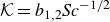 $\mathcal{K} = b_{1,2} {\textit{Sc}}^{-1/2}$
, where
$\mathcal{K} = b_{1,2} {\textit{Sc}}^{-1/2}$
, where $b_1= 0.012$
and
$b_1= 0.012$
and $b_2 = 0.021$
.
$b_2 = 0.021$
.

While the normalised value $\mathcal{K}^+=\mathcal{K}/\mathcal{K}_{Sc1}$
is useful to compare results obtained under very different conditions and to infer possible universal scaling laws, it is now interesting to turn our attention to the actual mass-transfer velocity
$\mathcal{K}^+=\mathcal{K}/\mathcal{K}_{Sc1}$
is useful to compare results obtained under very different conditions and to infer possible universal scaling laws, it is now interesting to turn our attention to the actual mass-transfer velocity $\mathcal{K}$
(i.e. not normalised by
$\mathcal{K}$
(i.e. not normalised by $\mathcal{K}_{Sc1}$
). This is shown in figure 8. As expected, results can be conveniently parametrised as
$\mathcal{K}_{Sc1}$
). This is shown in figure 8. As expected, results can be conveniently parametrised as $\mathcal{K} = b {\textit{Sc}}^{-1/2}$
. However, the value of the prefactor
$\mathcal{K} = b {\textit{Sc}}^{-1/2}$
. However, the value of the prefactor $b$
does depend on the specific case considered:
$b$
does depend on the specific case considered: $b=0.012$
for
$b=0.012$
for $D_r=1$
(case A), while
$D_r=1$
(case A), while $b=0.021$
for
$b=0.021$
for $D_r\gt 1$
(case B). This highlight the enhanced efficiency of the mass-transfer process when the mass diffusivity inside the drop is larger than outside of the drop. In particular, the ratio between the mass-transfer velocity is
$D_r\gt 1$
(case B). This highlight the enhanced efficiency of the mass-transfer process when the mass diffusivity inside the drop is larger than outside of the drop. In particular, the ratio between the mass-transfer velocity is $\mathcal{K}_{D_r\gt 1}/\mathcal{K}_{D_r=1} \simeq 1.75$
. We note that grid convergence tests performed on a reduced domain (Appendix A.3) indicate uncertainties of approximately 10 %–20 % in the predicted mass-transfer velocity at the highest Schmidt number considered (
$\mathcal{K}_{D_r\gt 1}/\mathcal{K}_{D_r=1} \simeq 1.75$
. We note that grid convergence tests performed on a reduced domain (Appendix A.3) indicate uncertainties of approximately 10 %–20 % in the predicted mass-transfer velocity at the highest Schmidt number considered ( ${\textit{Sc}}=4$
). While the qualitative scaling
${\textit{Sc}}=4$
). While the qualitative scaling $\mathcal{K} \propto {\textit{Sc}}^{-1/2}$
is robust across all grid resolutions tested, quantitative predictions at high
$\mathcal{K} \propto {\textit{Sc}}^{-1/2}$
is robust across all grid resolutions tested, quantitative predictions at high ${\textit{Sc}}$
should be interpreted with this level of uncertainty in mind. This results is in agreement with the two-film model of Liss & Slater (Reference Liss and Slater1974), in which the total resistance to the mass transfer is the sum of the resistance in either phase, leading to a mass-transfer velocity
${\textit{Sc}}$
should be interpreted with this level of uncertainty in mind. This results is in agreement with the two-film model of Liss & Slater (Reference Liss and Slater1974), in which the total resistance to the mass transfer is the sum of the resistance in either phase, leading to a mass-transfer velocity $\mathcal{K}$
(Wanninkhof et al. Reference Wanninkhof, Asher, Ho, Sweeney and McGillis2009):
$\mathcal{K}$
(Wanninkhof et al. Reference Wanninkhof, Asher, Ho, Sweeney and McGillis2009):
 \begin{equation} \frac {1}{\mathcal{K}} = \frac {1}{\mathcal{K}_d} + \frac {1}{\mathcal{K}_c} ,\end{equation}
with $\mathcal{K}_d$
and
$\mathcal{K}_d$
and $\mathcal{K}_c$
the mass-transfer velocities through the diffusive sublayers in the dispersed-phase side and carrier-phase side of the interface, respectively. Since
$\mathcal{K}_c$
the mass-transfer velocities through the diffusive sublayers in the dispersed-phase side and carrier-phase side of the interface, respectively. Since $\mathcal{K} \propto {\textit{Sc}}^{1/2}$
, we have
$\mathcal{K} \propto {\textit{Sc}}^{1/2}$
, we have $1/\mathcal{K} \propto \sqrt {{\textit{Sc}}_d}+\sqrt {{\textit{Sc}}_c}$
, thereby giving
$1/\mathcal{K} \propto \sqrt {{\textit{Sc}}_d}+\sqrt {{\textit{Sc}}_c}$
, thereby giving $\mathcal{K}_{D_r\gt 1}/\mathcal{K}_{D_r=1} = (1.751,1.818, 1.886,1.904)$
, in agreement with the results found with the DNS.
$\mathcal{K}_{D_r\gt 1}/\mathcal{K}_{D_r=1} = (1.751,1.818, 1.886,1.904)$
, in agreement with the results found with the DNS.
6. Conclusions
In this work, we have used a combined DNS–VOF approach to study the mass-transfer process in a wall-bounded turbulent channel flow. All drops are initially fully saturated with a given chemical species (i.e. initial species concentration $c_d=1$
), and are injected into the turbulent channel flow, where the chemical species is initially absent (i.e. initial species concentration
$c_d=1$
), and are injected into the turbulent channel flow, where the chemical species is initially absent (i.e. initial species concentration $c_c=0$
). Because of the given set-up, a net mass transfer (flux of chemical species) from the drops to the carrier flow is established. Three main physical parameters control the process: the Schmidt number
$c_c=0$
). Because of the given set-up, a net mass transfer (flux of chemical species) from the drops to the carrier flow is established. Three main physical parameters control the process: the Schmidt number ${\textit{Sc}}$
(momentum to mass diffusivity ratio), the bulk Reynolds number
${\textit{Sc}}$
(momentum to mass diffusivity ratio), the bulk Reynolds number ${\textit{Re}}_b$
(inertia to viscous forces ratio) and the Weber number
${\textit{Re}}_b$
(inertia to viscous forces ratio) and the Weber number ${\textit{We}}$
(inertia to surface tension forces ratio). In the present study, we kept
${\textit{We}}$
(inertia to surface tension forces ratio). In the present study, we kept ${\textit{Re}}$
and
${\textit{Re}}$
and ${\textit{We}}$
constant and equal to
${\textit{We}}$
constant and equal to ${\textit{Re}}_b=10\,000$
and
${\textit{Re}}_b=10\,000$
and ${We}=3100$
, and we varied
${We}=3100$
, and we varied ${\textit{Sc}}$
. Two different sets of numerical simulations have been performed, labelled case A and case B, respectively. In case A simulations, the Schmidt number in the carrier flow,
${\textit{Sc}}$
. Two different sets of numerical simulations have been performed, labelled case A and case B, respectively. In case A simulations, the Schmidt number in the carrier flow, ${\textit{Sc}}_c$
, is varied between
${\textit{Sc}}_c$
, is varied between ${\textit{Sc}}_c=0.5$
and
${\textit{Sc}}_c=0.5$
and ${\textit{Sc}}_c=4$
, and is set to be equal to the Schmidt number inside the drops,
${\textit{Sc}}_c=4$
, and is set to be equal to the Schmidt number inside the drops, ${\textit{Sc}}_d={\textit{Sc}}_c$
, finally giving a diffusivity ratio
${\textit{Sc}}_d={\textit{Sc}}_c$
, finally giving a diffusivity ratio $D_r={\textit{Sc}}_c/{\textit{Sc}}_d=1$
. In case B simulations, the Schmidt number in the carrier flow is varied between
$D_r={\textit{Sc}}_c/{\textit{Sc}}_d=1$
. In case B simulations, the Schmidt number in the carrier flow is varied between ${\textit{Sc}}_c=0.5$
and
${\textit{Sc}}_c=0.5$
and ${\textit{Sc}}_c=4$
, while the Schmidt number inside the drops is kept constant,
${\textit{Sc}}_c=4$
, while the Schmidt number inside the drops is kept constant, ${\textit{Sc}}_d=0.01$
, so that the diffusivity ratio is systematically increased between
${\textit{Sc}}_d=0.01$
, so that the diffusivity ratio is systematically increased between $D_r=50$
and
$D_r=50$
and $D_r=400$
. We analysed the behaviour of the average species concentration inside the drops,
$D_r=400$
. We analysed the behaviour of the average species concentration inside the drops, $\overline {c}_d$
, and inside the carrier flow,
$\overline {c}_d$
, and inside the carrier flow, $\overline {c}_c$
, and we showed that
$\overline {c}_c$
, and we showed that $\overline {c}_d$
decreases in time, while
$\overline {c}_d$
decreases in time, while $\overline {c}_c$
increases in time, until reaching an equilibrium condition
$\overline {c}_c$
increases in time, until reaching an equilibrium condition $\overline {c}_d \simeq \overline {c}_c$
. We also showed that fairly accurate predictions of the time behaviour of the concentration profiles can be obtained by a simplified lumped-parameter model. In addition, we focused on the behaviour of the mass-transfer velocity
$\overline {c}_d \simeq \overline {c}_c$
. We also showed that fairly accurate predictions of the time behaviour of the concentration profiles can be obtained by a simplified lumped-parameter model. In addition, we focused on the behaviour of the mass-transfer velocity $\mathcal{K}$
, which quantifies the rate at which mass is transferred across the interface. Our results consistently showed that
$\mathcal{K}$
, which quantifies the rate at which mass is transferred across the interface. Our results consistently showed that $\mathcal{K} \propto {\textit{Sc}}^{-1/2}$
for both case A simulations (i.e. when
$\mathcal{K} \propto {\textit{Sc}}^{-1/2}$
for both case A simulations (i.e. when $D_r=1$
) and case B simulations (i.e. when
$D_r=1$
) and case B simulations (i.e. when $D_r\gt 1$
), in good agreement with previous literature results covering a broad spectrum of scenarios (gas–liquid and liquid–liquid). These findings seem to highlight the universal nature of the mass-transfer process through deformable interfaces, no matter the specific flow configuration. While the scaling of the mass-transfer velocity with
$D_r\gt 1$
), in good agreement with previous literature results covering a broad spectrum of scenarios (gas–liquid and liquid–liquid). These findings seem to highlight the universal nature of the mass-transfer process through deformable interfaces, no matter the specific flow configuration. While the scaling of the mass-transfer velocity with ${\textit{Sc}}$
is robust and does not depend on the diffusivity ratio
${\textit{Sc}}$
is robust and does not depend on the diffusivity ratio $D_r$
, following the law
$D_r$
, following the law $\mathcal{K} \propto {\textit{Sc}}^{-1/2}$
, the magnitude of the mass-transfer velocity does depends on the diffusivity ratio. In particular, we found that
$\mathcal{K} \propto {\textit{Sc}}^{-1/2}$
, the magnitude of the mass-transfer velocity does depends on the diffusivity ratio. In particular, we found that $\mathcal{K}_{D_r\gt 1}/\mathcal{K}_{D_r=1} \simeq 1.75$
, a result that highlights the key role of the diffusivity ratio in enhancing the mass-transfer velocity.
$\mathcal{K}_{D_r\gt 1}/\mathcal{K}_{D_r=1} \simeq 1.75$
, a result that highlights the key role of the diffusivity ratio in enhancing the mass-transfer velocity.
Such insights could be critical for the design of more efficient systems in applications where liquid–liquid interactions are pivotal, potentially influencing operational strategies in chemical processing, waste treatment and other industrial applications. Furthermore, the implications of these findings can extend into environmental/geophysical fields. Understanding the drop-mediated gas exchange at the ocean surface, as a function of the diffusivity ratio, can enhance the future ability to model and predict the behaviour of gases in natural water bodies and the atmosphere. This is particularly relevant in studying the transport and fate of greenhouse gases and pollutants, providing crucial data that can inform environmental policy and strategies to mitigate climate change.
Acknowledgements
The results reported in this paper have been achieved using the EuroHPC Research Infrastructure resource LEONARDO based at CINECA, Casalecchio di Reno, Italy, under project EuroHPC R0387.
Funding
The authors gratefully acknowledge financial support from European Union-NextGenerationEU PNRR M4.C2.1.1-PRIN 2022, ‘The fluid dynamics of interfaces: mesoscale models for bubbles, drops, and membranes and their coupling to large scale flows’ 2022R9B2MW-G53C24000810001.
Declaration of interests
The authors report no conflict of interest.
Appendix A. Validation
In this appendix we validate our numerical set-up for the case of diffusion from a static and from a rising bubble.
A.1. Diffusion from a static bubble
Following previous works (see e.g. Farsoiya et al. Reference Farsoiya, Popinet and Deike2021), we benchmark our numerical implementation considering the diffusion from a stationary spherical bubble of constant size. Consider a stationary, axisymmetric bubble with radius $R_0 = d_0 / 2$
. Let
$R_0 = d_0 / 2$
. Let $D_g$
and
$D_g$
and $D_l$
denote the diffusivities in the gas and liquid phases, respectively. The one-dimensional transient concentration diffusion in spherical coordinates, both inside and outside the bubble, is described by
$D_l$
denote the diffusivities in the gas and liquid phases, respectively. The one-dimensional transient concentration diffusion in spherical coordinates, both inside and outside the bubble, is described by
 \begin{align} c_b(t, r) &= -\frac {2 c_{g0}}{\pi r} \int _0^\infty \frac {1}{x} \, {\rm Im} \left \{ \frac {\sinh \left [ \lambda _g(-x) \, r \right ]}{\zeta (-x)} \right \} {\rm e}^{-x t} \, \text{d}x, \end{align}
 \begin{align} c_l(t, r) &= \frac {c_{g0}}{\pi r} \int _0^\infty \frac {1}{x} \, {\rm Im} \left \{ \frac {\xi (-x)}{\zeta (-x)} {\rm e}^{ -\lambda _l(-x) \, r } \right \} {\rm e}^{-x t} \, \text{d}x, \end{align}
where ${\rm Im} (\boldsymbol{\cdot })$
denotes the imaginary part of a complex number. The derivation of these equations can be found in Farsoiya et al. (Reference Farsoiya, Popinet and Deike2021). Together with the analytical predictions, here we also present our numerical solutions for the transient species concentration both inside and outside of the spherical bubble. Note that solute concentrations are expressed as integrals, and are evaluated numerically. For this test, we consider a static bubble with a diameter of
${\rm Im} (\boldsymbol{\cdot })$
denotes the imaginary part of a complex number. The derivation of these equations can be found in Farsoiya et al. (Reference Farsoiya, Popinet and Deike2021). Together with the analytical predictions, here we also present our numerical solutions for the transient species concentration both inside and outside of the spherical bubble. Note that solute concentrations are expressed as integrals, and are evaluated numerically. For this test, we consider a static bubble with a diameter of $d_0/L=0.2$
, a diffusivity ratio of
$d_0/L=0.2$
, a diffusivity ratio of $D_g/D_l=10$
and a solubility
$D_g/D_l=10$
and a solubility $\alpha = 10^{-3}$
. Figures 9(a) and 9(b) show the transient concentrations inside the bubble at
$\alpha = 10^{-3}$
. Figures 9(a) and 9(b) show the transient concentrations inside the bubble at $r/d_0=0.25$
and outside the bubble at
$r/d_0=0.25$
and outside the bubble at $r/d_0=0.75$
, respectively. Together with the analytical solution (solid line), we also show our numerical predictions for different grid resolutions (coloured symbols). Convergence to the analytical prediction is clearly assessed. To highlight the prediction error of gas exchange through static bubbles, figure 9(c) shows the solute concentration error (
$r/d_0=0.75$
, respectively. Together with the analytical solution (solid line), we also show our numerical predictions for different grid resolutions (coloured symbols). Convergence to the analytical prediction is clearly assessed. To highlight the prediction error of gas exchange through static bubbles, figure 9(c) shows the solute concentration error ( $\epsilon (c_l)$
), defined as the difference between the predicted solute concentration outside the bubbles at a fixed time and the analytical solution, as a function of the number of grid points per bubble diameter.
$\epsilon (c_l)$
), defined as the difference between the predicted solute concentration outside the bubbles at a fixed time and the analytical solution, as a function of the number of grid points per bubble diameter.
Diffusion from a static bubble, comparing the numerical results with analytical trend and simulation by Farsoiya et al. (Reference Farsoiya, Popinet and Deike2021). (a) Concentration inside the bubble at $r/d_0 = 0.25$
. (b) Concentration outside the bubble at
$r/d_0 = 0.25$
. (b) Concentration outside the bubble at $r/d_0 = 0.75$
. (c) Error (
$r/d_0 = 0.75$
. (c) Error ( $\epsilon$
) (i.e. difference between numerical and analytical predictions) of the concentration outside of the bubble.
$\epsilon$
) (i.e. difference between numerical and analytical predictions) of the concentration outside of the bubble.

A.2. Diffusion from a rising bubble
To further assess our numerical method, and in particular to validate the advection–diffusion scheme, we examine the case of mass diffusion from a bubble rising (under the influence of buoyancy) in a quiescent fluid. The computational set-up (and in particular the values of the Bond and Archimedes, or Morton, numbers) is prepared in accordance with previous literature studies (Darmana, Deen & Kuipers Reference Darmana, Deen and Kuipers2006; Roghair Reference Roghair2012; Deising, Marschall & Bothe Reference Deising, Marschall and Bothe2016; Jia, Xiao & Kang Reference Jia, Xiao and Kang2019; Farsoiya et al. Reference Farsoiya, Popinet and Deike2021). The bubble rise velocity in a still liquid depends on the fluid and bubble properties, i.e. on the Archimedes number $Ar= g d_0^3 \rho _l (\rho _l - \rho _g ) \mu _l^2$
, the Morton number
$Ar= g d_0^3 \rho _l (\rho _l - \rho _g ) \mu _l^2$
, the Morton number $Mo=g\mu _l^4 /{} ( \rho _l \gamma ^3 \sigma )$
and the Bond number
$Mo=g\mu _l^4 /{} ( \rho _l \gamma ^3 \sigma )$
and the Bond number $Bo = \rho _l g d_0^2 \sigma$
(Moore Reference Moore1965; Maxworthy et al. Reference Maxworthy, Gnann, Kürten and Durst1996; Clift et al. Reference Clift, Grace and Weber2005; Cano-Lozano et al. Reference Cano-Lozano, Martinez-Bazan, Magnaudet and Tchoufag2016), and can be expressed via the non-dimensional bubble Reynolds number
$Bo = \rho _l g d_0^2 \sigma$
(Moore Reference Moore1965; Maxworthy et al. Reference Maxworthy, Gnann, Kürten and Durst1996; Clift et al. Reference Clift, Grace and Weber2005; Cano-Lozano et al. Reference Cano-Lozano, Martinez-Bazan, Magnaudet and Tchoufag2016), and can be expressed via the non-dimensional bubble Reynolds number ${\textit{Re}} = \rho _l U d_0 /\mu _l$
(Moore Reference Moore1965; Clift et al. Reference Clift, Grace and Weber2005). We evaluate two different configurations, corresponding to
${\textit{Re}} = \rho _l U d_0 /\mu _l$
(Moore Reference Moore1965; Clift et al. Reference Clift, Grace and Weber2005). We evaluate two different configurations, corresponding to ${\textit{Re}}=5.6$
and
${\textit{Re}}=5.6$
and ${\textit{Re}}=32.9$
, with Bond numbers
${\textit{Re}}=32.9$
, with Bond numbers $Bo=1$
and
$Bo=1$
and $Bo=40$
, and Archimedes numbers
$Bo=40$
, and Archimedes numbers $Ar=100$
and
$Ar=100$
and $Ar=8000$
. We follow Deike, Melville & Popinet (Reference Deike, Melville and Popinet2016) and we compute the mass transfer at Schmidt number
$Ar=8000$
. We follow Deike, Melville & Popinet (Reference Deike, Melville and Popinet2016) and we compute the mass transfer at Schmidt number ${\textit{Sc}}=\mu _l/ D_l=1$
and gas solubility
${\textit{Sc}}=\mu _l/ D_l=1$
and gas solubility $\alpha =1/30$
. The mass-transfer rate
$\alpha =1/30$
. The mass-transfer rate $\mathcal{K}$
is determined as
$\mathcal{K}$
is determined as
 \begin{equation} \mathcal{K} = \frac { \mathrm{d} c_g / \mathrm{d} t}{ A_g \left ( \alpha \bar {c}_g - \bar {c}_l \right ) }, \end{equation}
where $A_g$
is the instantaneous surface area of the bubble. Note that the solute concentration inside and outside the bubble is calculated as
$A_g$
is the instantaneous surface area of the bubble. Note that the solute concentration inside and outside the bubble is calculated as $c_g = \bar {c}_g V_g$
and
$c_g = \bar {c}_g V_g$
and $c_l = \bar {c}_l V_l$
, where
$c_l = \bar {c}_l V_l$
, where $\bar {c}_g$
and
$\bar {c}_g$
and $\bar {c}_l$
are defined in (4.1), and
$\bar {c}_l$
are defined in (4.1), and $V_g$
and
$V_g$
and $V_l$
represent the bubble and liquid volumes, respectively. Simulations are conducted using symmetric boundary conditions, modelling only one-quarter of the bubble, with a resolution of
$V_l$
represent the bubble and liquid volumes, respectively. Simulations are conducted using symmetric boundary conditions, modelling only one-quarter of the bubble, with a resolution of $d_0/\Delta x = 25.6$
. The results, shown in figure 10, are benchmarked against previous works. Figure 10(a) illustrates the time evolution of the non-dimensional transfer rate,
$d_0/\Delta x = 25.6$
. The results, shown in figure 10, are benchmarked against previous works. Figure 10(a) illustrates the time evolution of the non-dimensional transfer rate, ${Sh}=\mathcal{K} d_0/D_l$
, for both cases, with the mean steady-state values indicated by dashed lines. Figure 10(b) compares the values of
${Sh}=\mathcal{K} d_0/D_l$
, for both cases, with the mean steady-state values indicated by dashed lines. Figure 10(b) compares the values of ${\textit{Sh}}$
obtained by current computations with previous literature results. The theoretical prediction
${\textit{Sh}}$
obtained by current computations with previous literature results. The theoretical prediction ${Sh}=2/\sqrt {\pi } Pe$
proposed by Levich (Reference Levich1962) is also shown for comparison purposes. Our findings demonstrate that the proposed method produces results consistent with previous studies and aligns well with theoretical predictions.
${Sh}=2/\sqrt {\pi } Pe$
proposed by Levich (Reference Levich1962) is also shown for comparison purposes. Our findings demonstrate that the proposed method produces results consistent with previous studies and aligns well with theoretical predictions.
Diffusion from a rising bubble, comparing the numerical results with analytical trend and simulation by Roghair (Reference Roghair2012), Deising et al. (Reference Deising, Bothe and Marschall2018) and Farsoiya et al. Reference Farsoiya, Popinet and Deike2021). (a) Evolution with time of non-dimensional transfer rates, with Levich (Reference Levich1962) predicted values (dashed lines). (b) Steady-state transfer rate as a function of Péclet number compared against Levich (Reference Levich1962).

A.3. Grid sensitivity analysis
As a further benchmark, we performed a grid sensitivity analysis on a turbulent flow case. In particular, we performed a series of simulations of a turbulent channel flow with the injection of drops that are initially fully saturated with a given chemical species. This set-up is similar to the one used to run the simulations presented in the main body of this paper. However, in this case, the channel dimensions are $L_x \times L_y \times L_z = \pi h \times 2 h \times \pi /2 h$
, i.e. four times smaller than the full channel discussed in the main body of the paper. Even for the present test, we run case A and case B simulations (i.e. case A with unitary diffusivity ratio
$L_x \times L_y \times L_z = \pi h \times 2 h \times \pi /2 h$
, i.e. four times smaller than the full channel discussed in the main body of the paper. Even for the present test, we run case A and case B simulations (i.e. case A with unitary diffusivity ratio $D_r=1$
and case B with
$D_r=1$
and case B with $D_r \gg 1$
). We employed three different grid resolutions: coarse (
$D_r \gg 1$
). We employed three different grid resolutions: coarse ( $144 \times 144 \times 72$
), medium (
$144 \times 144 \times 72$
), medium ( $288 \times 288 \times 144$
) and fine (
$288 \times 288 \times 144$
) and fine ( $576 \times 576 \times 288$
), which correspond, respectively, to half, identical and double resolution compared with the full-channel simulations analysed in the main body of the paper. In these test cases, we considered five different Schmidt numbers of the carrier phase:
$576 \times 576 \times 288$
), which correspond, respectively, to half, identical and double resolution compared with the full-channel simulations analysed in the main body of the paper. In these test cases, we considered five different Schmidt numbers of the carrier phase: ${\textit{Sc}}_c = 0.5,\ 1,\ 2,\ 4,\ 8$
.
${\textit{Sc}}_c = 0.5,\ 1,\ 2,\ 4,\ 8$
.
Figure 11 shows the mass-transfer velocity $\mathcal{K}$
as a function of Schmidt number (figure 11
a) and the relative error
$\mathcal{K}$
as a function of Schmidt number (figure 11
a) and the relative error $\epsilon$
in the mass-transfer velocity with respect to the finest grid (figure 11
b). This test also includes
$\epsilon$
in the mass-transfer velocity with respect to the finest grid (figure 11
b). This test also includes ${\textit{Sc}} = 8$
, which was not analysed in the full-channel simulations. We observe that the scaling law
${\textit{Sc}} = 8$
, which was not analysed in the full-channel simulations. We observe that the scaling law $\mathcal{K} \propto {\textit{Sc}}^{-1/2}$
is predicted fairly well by both medium and fine grid resolutions, while the coarse grid resolution fails to reproduce it accurately for Schmidt numbers
$\mathcal{K} \propto {\textit{Sc}}^{-1/2}$
is predicted fairly well by both medium and fine grid resolutions, while the coarse grid resolution fails to reproduce it accurately for Schmidt numbers ${\textit{Sc}}\gt 2$
. The absolute error in mass-transfer velocity
${\textit{Sc}}\gt 2$
. The absolute error in mass-transfer velocity $\epsilon$
demonstrates improved accuracy with increasing resolution, ranging from approximately 1 % error at lower Schmidt numbers to about 10 %–20 % error at
$\epsilon$
demonstrates improved accuracy with increasing resolution, ranging from approximately 1 % error at lower Schmidt numbers to about 10 %–20 % error at ${\textit{Sc}}=4$
.
${\textit{Sc}}=4$
.
Grid sensitivity analysis results from simulations of a reduced channel (four times smaller than the one analysed in the main body of the paper) used as a reference test. Coarse grid, $\Delta x^+=6.54$
; medium grid,
$\Delta x^+=6.54$
; medium grid, $\Delta x^+= 3.27$
; fine grid,
$\Delta x^+= 3.27$
; fine grid, $\Delta x^+=1.635$
. Label A refers to simulations with diffusivity ratio
$\Delta x^+=1.635$
. Label A refers to simulations with diffusivity ratio $D_r=1$
, while label B refers to simulations with diffusivity ratio
$D_r=1$
, while label B refers to simulations with diffusivity ratio $D_r=(50,100,200,400,800)$
. (a) Scaling of gas-transfer velocity,
$D_r=(50,100,200,400,800)$
. (a) Scaling of gas-transfer velocity, $\mathcal{K}$
, as a function of Schmidt number,
$\mathcal{K}$
, as a function of Schmidt number, ${\textit{Sc}}$
. (b) Relative error,
${\textit{Sc}}$
. (b) Relative error, $\epsilon$
, of
$\epsilon$
, of $\mathcal{K}$
with respect to the fine-grid results.
$\mathcal{K}$
with respect to the fine-grid results.

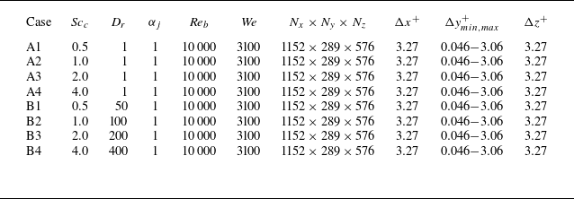


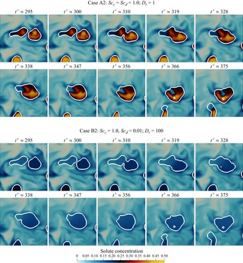


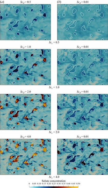


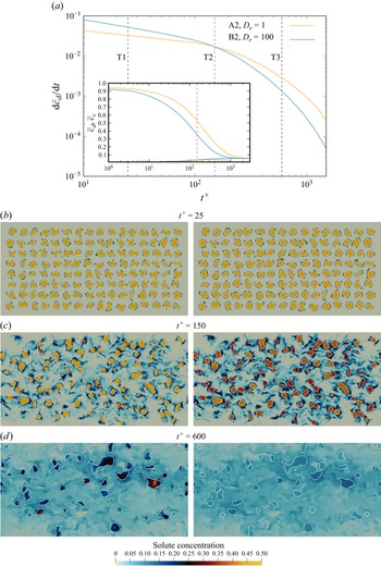


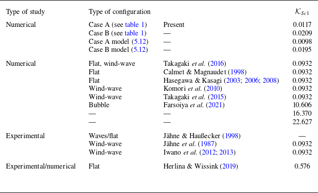


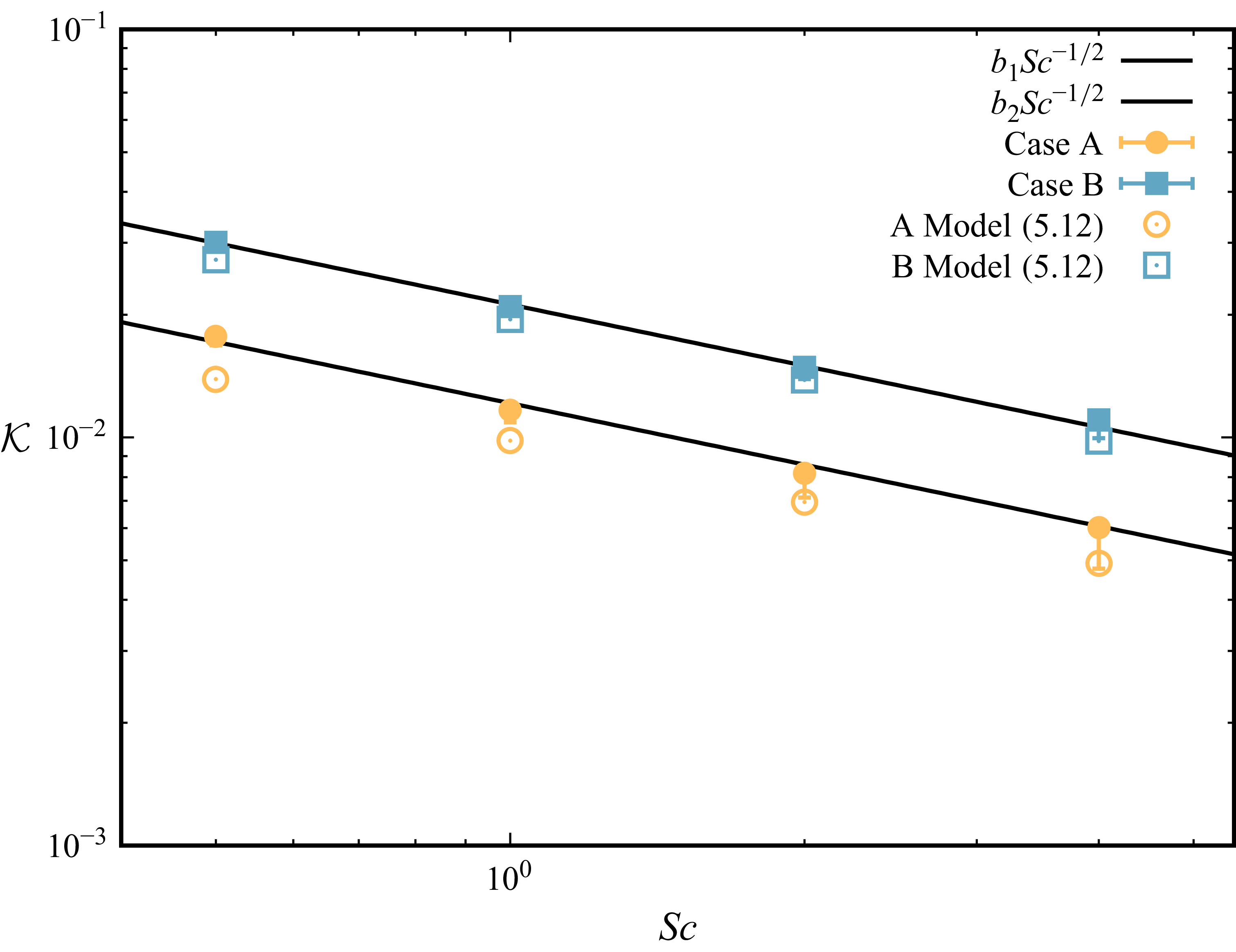


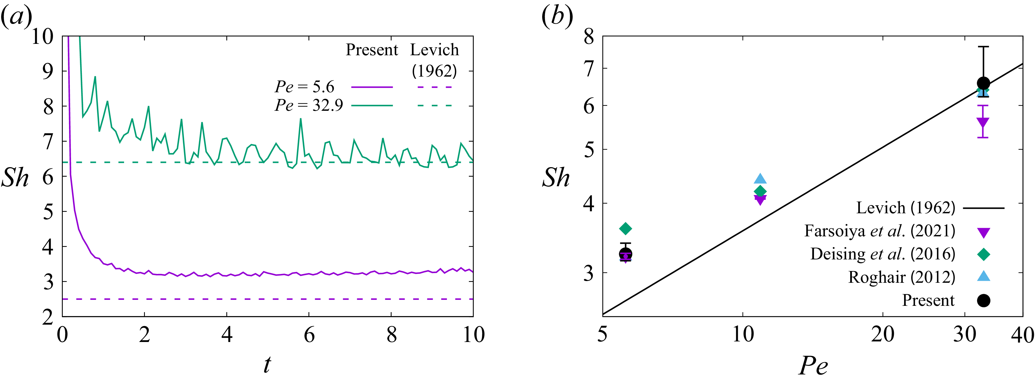
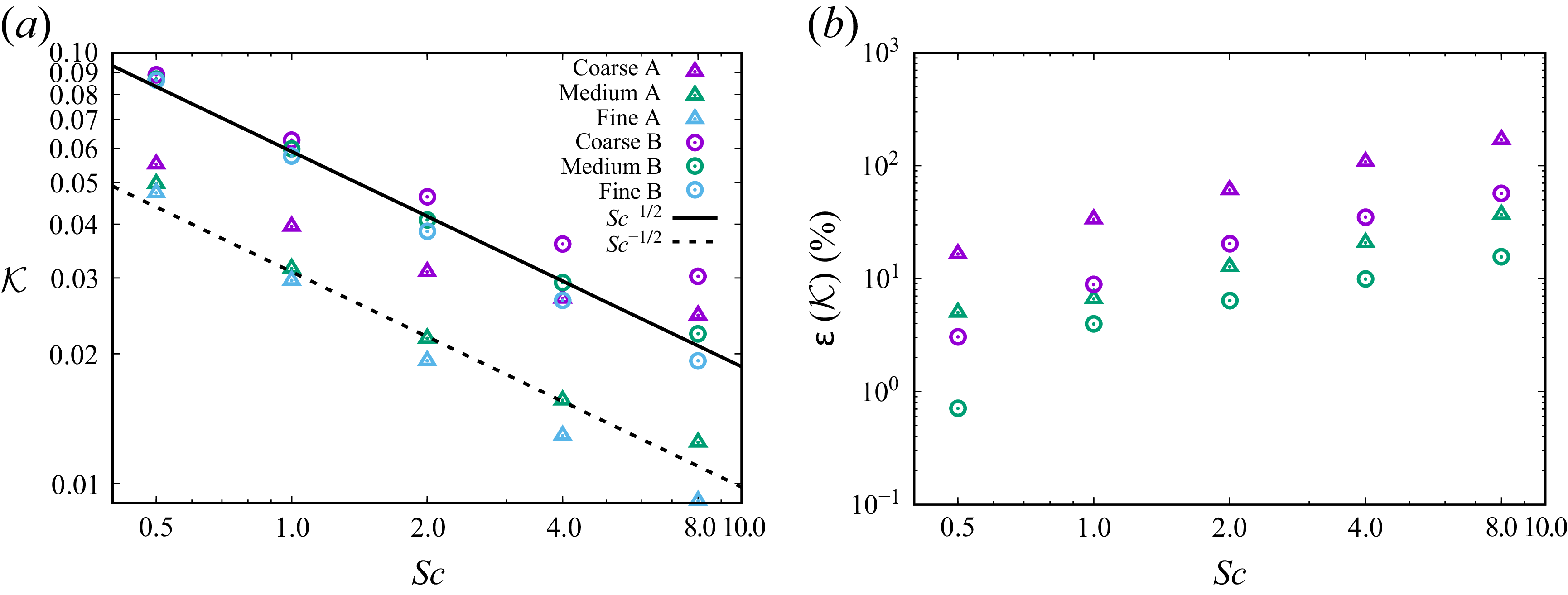


 Open access

