





1. Introduction
Geothermal heating of the Earth’s oceans has a flux Rayleigh number of order $10^{24}$
(see Appendix A). This strongly supercritical bottom heating does not result in Rayleigh–Bénard convection (RBC). Instead, ocean stratification is reliably stable – even strongly stable in the sense that the buoyancy frequency is greater than the Coriolis frequency almost everywhere. Suppression of geothermally forced RBC indicates the importance of horizontal convection (Rossby Reference Rossby1965, Reference Rossby1998; Hughes & Griffiths Reference Hughes and Griffiths2008) associated with a sea-surface pole-to-equator temperature difference of order
$10^{24}$
(see Appendix A). This strongly supercritical bottom heating does not result in Rayleigh–Bénard convection (RBC). Instead, ocean stratification is reliably stable – even strongly stable in the sense that the buoyancy frequency is greater than the Coriolis frequency almost everywhere. Suppression of geothermally forced RBC indicates the importance of horizontal convection (Rossby Reference Rossby1965, Reference Rossby1998; Hughes & Griffiths Reference Hughes and Griffiths2008) associated with a sea-surface pole-to-equator temperature difference of order $30$
K. Horizontal convection (HC), assisted by wind and tides, produces a stably stratified ocean (Munk & Wunsch Reference Munk and Wunsch1998). Impelled by observations of stable ocean stratification, oceanographers are concerned only with secondary effects of geothermal heating, such as modification of abyssal water masses (e.g. Emile-Geay & Madec Reference Emile-Geay and Madec2009; De Lavergne et al. Reference De Lavergne, Madec, Le Sommer, Nurser and Naveira Garabato2016) or the possibility that geothermal heating enhances the strength of the meridional overturning circulation (e.g. Mullarney, Griffiths & Hughes Reference Mullarney, Griffiths and Hughes2006; Wang et al. Reference Wang, Huang, Zhou and Xia2016).
$30$
K. Horizontal convection (HC), assisted by wind and tides, produces a stably stratified ocean (Munk & Wunsch Reference Munk and Wunsch1998). Impelled by observations of stable ocean stratification, oceanographers are concerned only with secondary effects of geothermal heating, such as modification of abyssal water masses (e.g. Emile-Geay & Madec Reference Emile-Geay and Madec2009; De Lavergne et al. Reference De Lavergne, Madec, Le Sommer, Nurser and Naveira Garabato2016) or the possibility that geothermal heating enhances the strength of the meridional overturning circulation (e.g. Mullarney, Griffiths & Hughes Reference Mullarney, Griffiths and Hughes2006; Wang et al. Reference Wang, Huang, Zhou and Xia2016).
We refer to the production of stable interior stratification in a bottom-heated fluid layer as ‘restratification’. As a definition, we say that the fluid is restratified if the volume average of the vertical buoyancy gradient – $\langle b_z\rangle$
in the notation of § 2 – is positive. Figure 1 shows an example of restratification: in the HC + RBC configuration the volume-averaged vertical buoyancy gradient
$\langle b_z\rangle$
in the notation of § 2 – is positive. Figure 1 shows an example of restratification: in the HC + RBC configuration the volume-averaged vertical buoyancy gradient $\langle b_z\rangle$
is positive, despite bottom heating.
$\langle b_z\rangle$
is positive, despite bottom heating.
Geophysical convection problems involving restratification include the circulation of subglacial lakes (Thoma et al. Reference Thoma, Grosfeld, Filina and Mayer2009; Couston & Siegert Reference Couston and Siegert2021), the ocean of snowball Earth during the Neoproterozoic (Hoffman & Schrag Reference Hoffman and Schrag2002; Pierrehumbert et al. Reference Pierrehumbert, Abbot, Voigt and Koll2011) and the oceans of icy moons such as Europa and Enceladus (e.g. Soderlund Reference Soderlund2019; Lemasquerier, Bierson & Soderlund Reference Lemasquerier, Bierson and Soderlund2023). In these systems geothermal heating is essential in maintaining a liquid ocean beneath an ice sheet. The ice sheet has variable thickness, and therefore variable pressure and freezing temperature at its base. The non-uniform basal ice temperature results in HC, and perhaps restratification, in the geothermally heated water below. Other horizontal non-uniformities result from spatial variations in the bottom flux of heat, salinity fluxes from the freezing and melting of ice and non-uniform depth of the water layer.
The oceans of icy moons and of snowball Earth differ from the Earth’s present ocean in that there is no sea-surface forcing by wind stress. Wind stress is the main source of energy for ocean circulation (Munk & Wunsch Reference Munk and Wunsch1998; Wunsch & Ferrari Reference Wunsch and Ferrari2004). It is likely therefore that the circulation of icy-moon oceans differs qualitatively from that of Earth: observations of ubiquitous statically stable stratification in the Earth’s present ocean are not a reliable guide to stratification in other bottom-heated oceans.
Investigations of snowball Earth and icy moons make diverse and contradictory assumptions regarding the competition between RBC and HC in these systems. For example, Jansen (Reference Jansen2016) assumes that horizontal inhomogeneities in snowball Earth heat fluxes result in statically stable stratification. In Jansen’s view, vertical heat fluxes, required to transmit geothermal heat to the base of the ice sheet, result from baroclinic instability (also known as slantwise convection) in a horizontally restratified ocean. On the other hand, Ashkenazy & Tziperman (Reference Ashkenazy and Tziperman2016) argue that the ocean of snowball Earth is, to a first approximation, well mixed vertically by geothermal RBC. In a numerical exploration of icy-moon ocean circulation, Bire et al. (Reference Bire, Kang, Ramadhan, Campin and Marshall2022) ignore horizontal inhomogeneities that might result in HC and focus instead on rotating RBC forced by unopposed uniform bottom heating. But in another exploration of icy-moon ocean circulation, Zhang, Kang & Marshall (Reference Zhang, Kang and Marshall2024) use an insulating bottom boundary condition (no RBC) and instead force with horizontally non-uniform temperature (i.e. HC) at the base of the ice sheet.
Models of icy-moon oceans are largely unconstrained by observations. For snowball Earth, our ignorance is even more profound and likely to remain so. It is essential therefore to identify the parameters determining whether the bulk stratification $\langle b_z\rangle$
of these oceans is statically stable. Subsequent modelling depends heavily on this issue. For example, a stably stratified ice-covered ocean might be energised by tidally generated internal waves resulting in turbulent interior mixing (e.g. Wunsch Reference Wunsch2016). Baroclinic instability occurs only if the bulk stratification is stable. Sufficiently strong stable stratification is the basis for the ‘traditional approximation’ in which only the component of the planetary vorticity in the direction parallel to the base-state buoyancy gradient is retained (e.g. Gerkema et al. Reference Gerkema, Zimmerman, Maas and Van Haren2008). In short, if
$\langle b_z\rangle$
of these oceans is statically stable. Subsequent modelling depends heavily on this issue. For example, a stably stratified ice-covered ocean might be energised by tidally generated internal waves resulting in turbulent interior mixing (e.g. Wunsch Reference Wunsch2016). Baroclinic instability occurs only if the bulk stratification is stable. Sufficiently strong stable stratification is the basis for the ‘traditional approximation’ in which only the component of the planetary vorticity in the direction parallel to the base-state buoyancy gradient is retained (e.g. Gerkema et al. Reference Gerkema, Zimmerman, Maas and Van Haren2008). In short, if $\langle b_z\rangle \gt 0$
then business-as-usual ocean modelling can proceed. If
$\langle b_z\rangle \gt 0$
then business-as-usual ocean modelling can proceed. If $\langle b_z\rangle \lt 0$
then a very different class of models, suggested by processes in a stellar convection zone, might be appropriate.
$\langle b_z\rangle \lt 0$
then a very different class of models, suggested by processes in a stellar convection zone, might be appropriate.
Horizontally and time-averaged vertical buoyancy gradient $\bar b_z(z)$
in three cases. The inset shows a snapshots of the buoyancy with overlaid streamlines. The HC Rayleigh number,
$\bar b_z(z)$
in three cases. The inset shows a snapshots of the buoyancy with overlaid streamlines. The HC Rayleigh number, $\mathit{Ra_H}$
, and the RBC flux Rayleigh number,
$\mathit{Ra_H}$
, and the RBC flux Rayleigh number, $\mathit{Ra_V}$
, are defined in (2.7); other parameters are
$\mathit{Ra_V}$
, are defined in (2.7); other parameters are $\varGamma =8$
and
$\varGamma =8$
and ${\textit{Pr}}=1$
defined in (2.8). For the joint HC and RBC case, the time and volume-averaged vertical buoyancy gradient is
${\textit{Pr}}=1$
defined in (2.8). For the joint HC and RBC case, the time and volume-averaged vertical buoyancy gradient is $\langle b_z \rangle /\beta =0.38$
, where
$\langle b_z \rangle /\beta =0.38$
, where $\beta \gt 0$
is defined in (2.1).
$\beta \gt 0$
is defined in (2.1).

Figure 1. Long description
The image contains a graph depicting the horizontally and time-averaged vertical buoyancy gradient in three cases. The graph includes three distinct lines representing different scenarios: horizontal convection (HC), combined horizontal convection and Rayleigh-Bénard convection (HC + RBC), and Rayleigh-Bénard convection (RBC). The x-axis represents the normalized vertical buoyancy gradient, while the y-axis represents the normalized height. The inset images show snapshots of buoyancy with overlaid streamlines for each scenario. The blue line represents HC with a Rayleigh number of 10^7 and zero vertical Rayleigh number. The green line represents HC + RBC with both Rayleigh numbers at 10^7. The red line represents RBC with zero horizontal Rayleigh number and a vertical Rayleigh number of 10^7. The insets visually illustrate the flow patterns and buoyancy distributions for each case, highlighting the differences in convection and stratification.
For both RBC and HC a key challenge is determining the relation between heat transport and surface forcing, i.e. the relation between Nusselt $Nu$
and Rayleigh
$Nu$
and Rayleigh ${Ra}$
numbers. While the
${Ra}$
numbers. While the $Nu$
–
$Nu$
– ${Ra}$
relation is not a goal of this investigation, related boundary-layer scaling arguments are useful in § 4. For the RBC boundary layer, see Grossmann & Lohse (2000, Reference Grossmann and Lohse2001), Doering (Reference Doering2020) and Lohse & Shishkina (Reference Lohse and Shishkina2024). For the HC boundary layer the literature is smaller: see Rossby (Reference Rossby1965, Reference Rossby1998), Shishkina, Grossmann & Lohse (Reference Shishkina, Grossmann and Lohse2016) and more recently Passaggia & Scotti (Reference Passaggia and Scotti2024) and Passaggia, Cohen & Scotti (Reference Passaggia, Cohen and Scotti2024).
${Ra}$
relation is not a goal of this investigation, related boundary-layer scaling arguments are useful in § 4. For the RBC boundary layer, see Grossmann & Lohse (2000, Reference Grossmann and Lohse2001), Doering (Reference Doering2020) and Lohse & Shishkina (Reference Lohse and Shishkina2024). For the HC boundary layer the literature is smaller: see Rossby (Reference Rossby1965, Reference Rossby1998), Shishkina, Grossmann & Lohse (Reference Shishkina, Grossmann and Lohse2016) and more recently Passaggia & Scotti (Reference Passaggia and Scotti2024) and Passaggia, Cohen & Scotti (Reference Passaggia, Cohen and Scotti2024).
Motivated by the dynamics of subglacial lakes, Couston, Nandaha & Favier (Reference Couston, Nandaha and Favier2022) (hereafter CNF) investigated the competition between RBC and HC and demonstrated a regime transition between the two varieties of convection. Close to the regime transition, and with flux Rayleigh number as large as $10^6$
, CNF showed that there is bistability and hysteresis: two stable flow states co-exist at the same parameter values. In one state RBC is dominant (multiple convection cells, most with a horizontal scale comparable to the layer depth) and in the other state HC dominates (fewer cells, most elongated in the horizontal direction). The history of the system determines which state is observed.
$10^6$
, CNF showed that there is bistability and hysteresis: two stable flow states co-exist at the same parameter values. In one state RBC is dominant (multiple convection cells, most with a horizontal scale comparable to the layer depth) and in the other state HC dominates (fewer cells, most elongated in the horizontal direction). The history of the system determines which state is observed.
Here, we use the RBC + HC set-up studied by CNF, focusing on the issue of restratification. Restratification indicates that the competition between RBC and HC is settled: RBC has capitulated and most of the fluid is statically stable with $\langle b_z\rangle$
having the positive sign characteristic of HC.
$\langle b_z\rangle$
having the positive sign characteristic of HC.
Geophysical situations present complications such as rotation, salinity and spherical shell geometry. But understanding restratification in the idealised RBC + HC model is a necessary prerequisite: we must first identify the non-dimensional parameters that determine the outcome of this competition in the relatively simple RBC + HC model.
Section 2 presents the governing equations, numerical set-up and control parameters. We define the two Rayleigh numbers that quantify the bottom buoyancy flux and the horizontal buoyancy forcing. Section 3 defines restratification, and § 4 examines the flow phenomenology and key scalings of two characteristic stratification configurations: neutral and strong stratification. Section 5 develops scaling arguments based on the dynamics of the top boundary layer and identifies its controlling role in the system. We derive scaling laws for the boundary-layer thickness and mean buoyancy in the asymptotic regimes in which RBC dominates HC and vice versa. The same framework is then used to determine the thresholds for the onset of neutral and strong stratification, establishing their dependence on the flux and horizontal Rayleigh numbers in both low- and high-Rayleigh-number regimes. Section 6 examines the sensitivity of the results to variations in the Prandtl number, compares them with the findings of CNF and explores the implications for geophysical systems where bottom heating and lateral buoyancy gradients interact. Section 7 concludes with directions for future work.
2. Formulation of the restratification problem
2.1. The Boussinesq equations
We consider a layer of Boussinesq fluid with depth $h$
and density
$h$
and density $\rho = \rho _{\textit{ref}} (1 - g^{-1}b)$
, where
$\rho = \rho _{\textit{ref}} (1 - g^{-1}b)$
, where $\rho _{\textit{ref}}$
is a constant reference density,
$\rho _{\textit{ref}}$
is a constant reference density, $g$
is the gravitational acceleration and
$g$
is the gravitational acceleration and $b$
is the ‘buoyancy’. If, for example, the fluid is stratified by temperature variations then
$b$
is the ‘buoyancy’. If, for example, the fluid is stratified by temperature variations then $b = g \alpha (T - T_{\textit{ref}})$
, where
$b = g \alpha (T - T_{\textit{ref}})$
, where $T_{\textit{ref}}$
is a reference temperature,
$T_{\textit{ref}}$
is a reference temperature, $\alpha$
is the thermal expansion coefficient and
$\alpha$
is the thermal expansion coefficient and $g$
is the gravitational acceleration.We define
$g$
is the gravitational acceleration.We define $T_{\textit{ref}}$
so that the horizontal and time average of
$T_{\textit{ref}}$
so that the horizontal and time average of $b$
prescribed at the top surface
$b$
prescribed at the top surface $z=h$
is zero.
$z=h$
is zero.
At the bottom, $z = 0$
, the buoyancy boundary condition is specified constant diffusive flux of buoyancy,
$z = 0$
, the buoyancy boundary condition is specified constant diffusive flux of buoyancy, $F$
defined in (A4), into the fluid. This is equivalent to the Neumann boundary condition
$F$
defined in (A4), into the fluid. This is equivalent to the Neumann boundary condition
 \begin{align} b_z(x,y,0,t) = - \beta , \end{align}
where $\beta = F/\kappa \gt 0$
, using the thermal diffusivity
$\beta = F/\kappa \gt 0$
, using the thermal diffusivity $\kappa$
. At the top of the layer,
$\kappa$
. At the top of the layer, $z = h$
, the boundary condition is
$z = h$
, the boundary condition is
 \begin{align} b(x,y,h,t) = b^{\textit{s}}(x,y), \end{align}
where the “surface buoyancy” $b^{\textit{s}}$
is a specified function of position, e.g. (2.6).
$b^{\textit{s}}$
is a specified function of position, e.g. (2.6).
With the notation above, the Boussinesq equations of motion are
 \begin{align} \boldsymbol{u}_t + \boldsymbol{u} \boldsymbol{\cdot } \boldsymbol{\nabla } \boldsymbol{u} + \boldsymbol{\nabla } p &= b \boldsymbol{\hat z} + \nu \boldsymbol{\nabla} ^2 \boldsymbol{u} , \end{align}
 \begin{align} b_t + \boldsymbol{u} \boldsymbol{\cdot } \boldsymbol{\nabla } b &= \kappa \boldsymbol{\nabla} ^2 b , \end{align}
 \begin{align} \boldsymbol{\nabla } \boldsymbol{\cdot } \boldsymbol{u} &= 0 ,\end{align}
where $u,p$
and
$u,p$
and $\nu$
are the velocity, the pressure and the kinematic viscosity, respectively. We impose no-slip boundary conditions on all solid boundaries. In two-dimensional numerical solutions, with
$\nu$
are the velocity, the pressure and the kinematic viscosity, respectively. We impose no-slip boundary conditions on all solid boundaries. In two-dimensional numerical solutions, with $-\ell _x/2 \lt x \lt + \ell _x/2$
, we use the sinusoidal profile
$-\ell _x/2 \lt x \lt + \ell _x/2$
, we use the sinusoidal profile
 \begin{align} b^{\textit{s}}(x) = - b_{\star } \cos k x , \end{align}
with $k = 2 \pi / \ell _x$
. In general one can introduce a buoyancy scale
$k = 2 \pi / \ell _x$
. In general one can introduce a buoyancy scale $b_{\star }$
as a dimensional measure of horizontal buoyancy variations specified at the top surface. We take
$b_{\star }$
as a dimensional measure of horizontal buoyancy variations specified at the top surface. We take $b_{\star }\gt 0$
so that the densest surface fluid is in the middle of the domain at
$b_{\star }\gt 0$
so that the densest surface fluid is in the middle of the domain at $x=0$
. The HC plume is then well away from the no-slip sidewalls at
$x=0$
. The HC plume is then well away from the no-slip sidewalls at $x=\pm \ell _x/2$
(see inset in figure 1). This set-up is illustrated in figure 2.
$x=\pm \ell _x/2$
(see inset in figure 1). This set-up is illustrated in figure 2.
Numerical solutions of (2.1) to (2.6) presented in §§ 4 and 5 are based on the two-dimensional (2-D) case with $\ell _y=0$
. The theoretical developments in § 3, however, apply equally well to the three-dimensional (3-D) case. And in § 6 we assess the effects of three-dimensionality by presenting numerical solutions with periodicity in the
$\ell _y=0$
. The theoretical developments in § 3, however, apply equally well to the three-dimensional (3-D) case. And in § 6 we assess the effects of three-dimensionality by presenting numerical solutions with periodicity in the $y$
-direction and
$y$
-direction and $\ell _y=h$
.
$\ell _y=h$
.
2.2. Non-dimensional control parameters
This problem is characterised by both a HC Rayleigh number and a vertical RBC flux Rayleigh number
 \begin{align} \mathit{Ra_H} \mathop {=}\limits ^{\mathit{def}} \frac {h^3 b_{\star }}{\nu \kappa } \qquad \textrm{and} \qquad \mathit{Ra_V} \mathop {=}\limits ^{\mathit{def}} \frac {h^4F}{\nu \kappa ^2} = \frac {h^4\beta }{\nu \kappa }. \end{align}
Additional non-dimensional parameters are the Prandtl number and aspect ratio
 \begin{align} {\textit{Pr}} \mathop {=}\limits ^{\mathit{def}} \frac {\nu }{\kappa } \qquad \textrm{and} \qquad \varGamma \mathop {=}\limits ^{\mathit{def}} \frac {\ell _x}{h}. \end{align}
Sketch of the two-dimensional fluid layer illustrating the boundary conditions. There is a uniform buoyancy flux, $F=\kappa \beta$
, through the bottom, non-uniform buoyancy at the top and no buoyancy flux through the sidewalls. All boundaries satisfy no-slip velocity conditions.
$F=\kappa \beta$
, through the bottom, non-uniform buoyancy at the top and no buoyancy flux through the sidewalls. All boundaries satisfy no-slip velocity conditions.

Figure 2. Long description
The diagram illustrates a two-dimensional fluid layer with various boundary conditions. A uniform buoyancy flux is applied through the bottom, while the top has non-uniform buoyancy and no buoyancy flux through the sidewalls. All boundaries satisfy no-slip velocity conditions. The fluid layer is bounded by insulated surfaces on the top and bottom, with specific conditions at the sidewalls. The diagram includes arrows indicating the direction of buoyancy flux and labels for the different boundary conditions.
The traditional definition of the HC Rayleigh number, introduced by Rossby (Reference Rossby1965, Reference Rossby1998), is based on the horizontal length $\ell _x$
and the total difference between the maximum and minimum imposed surface buoyancy. In our notation, and using the sinusoidal surface buoyancy profile in (2.6), this traditional HC Rayleigh number is
$\ell _x$
and the total difference between the maximum and minimum imposed surface buoyancy. In our notation, and using the sinusoidal surface buoyancy profile in (2.6), this traditional HC Rayleigh number is
 \begin{align} \mathit{Ra^{trad}_H} = \frac {2 b_{\star } \ell _x^3}{\nu \kappa } = 2 \varGamma ^3 \mathit{Ra_H}. \end{align}
Our unconventional definition of $\mathit{Ra_H}$
simplifies subsequent results. But because we consider largish aspect ratios (
$\mathit{Ra_H}$
simplifies subsequent results. But because we consider largish aspect ratios ( $\varGamma \geqslant 8$
) our
$\varGamma \geqslant 8$
) our $\mathit{Ra_H}$
is smaller than the corresponding
$\mathit{Ra_H}$
is smaller than the corresponding $\mathit{Ra^{trad}_H}$
by a factor of at least
$\mathit{Ra^{trad}_H}$
by a factor of at least $2^{10}$
. This factor
$2^{10}$
. This factor $2^{10}$
complicates comparison of our results with earlier studies of HC using
$2^{10}$
complicates comparison of our results with earlier studies of HC using $\mathit{Ra^{trad}_H}$
as a control parameter.
$\mathit{Ra^{trad}_H}$
as a control parameter.
We introduce non-dimensional variables denoted by a dash and defined by
 \begin{align}&\qquad (x,y,z) = h (x^\prime,y^\prime,z^\prime), \qquad t^\prime = \kappa t/h^2 , \end{align}
 \begin{align}& \boldsymbol{u}^\prime = h\boldsymbol{u}/\kappa , \qquad p^\prime = h^2 p/(\nu \kappa ) , \qquad b^\prime = h^3b/(\nu \kappa ) . \end{align}
Dropping the dash, the non-dimensional versions of (2.3) through (2.5) are
 \begin{align} {\textit{Pr}}^{-1}(\boldsymbol{u}_t + \boldsymbol{u} \boldsymbol{\cdot } \boldsymbol{\nabla } \boldsymbol{u}) &= -\boldsymbol{\nabla } p +b \boldsymbol{\hat z} + \boldsymbol{\nabla} ^2 \boldsymbol{u} , \end{align}
 \begin{align} b_t + \boldsymbol{u} \boldsymbol{\cdot } \boldsymbol{\nabla } b &= \boldsymbol{\nabla} ^2 b , \end{align}
 \begin{align} \boldsymbol{\nabla } \boldsymbol{\cdot } \boldsymbol{u} &= 0 . \end{align}
The non-dimensional versions of the boundary conditions in (2.1) and (2.6) are
 \begin{align} b(x,y,1,t) = - \mathit{Ra_H} \cos k x , \qquad b_z(x,y,0,t) = - \mathit{Ra_V}. \end{align}
The unconventional definition of non-dimensional variables in (2.10) and (2.11) ensures that Rayleigh numbers $\mathit{Ra_H}$
and
$\mathit{Ra_H}$
and $\mathit{Ra_V}$
appear on equal footing in the boundary conditions (2.15). Using
$\mathit{Ra_V}$
appear on equal footing in the boundary conditions (2.15). Using $\mathit{Ra_H}$
, rather than
$\mathit{Ra_H}$
, rather than $\mathit{Ra^{trad}_H}$
, ensures that the aspect ratio
$\mathit{Ra^{trad}_H}$
, ensures that the aspect ratio $\varGamma$
does not appear in the boundary conditions (2.15).
$\varGamma$
does not appear in the boundary conditions (2.15).
The governing equations (2.12–2.14), together with the boundary conditions (2.15), and no-slip conditions on all boundaries, are solved numerically in a 2-D box using the spectral-element code Nek5000 (Fischer Reference Fischer1997; Deville, Fischer & Mund Reference Deville, Fischer and Mund2002). This solver has been widely applied to studies of thermal convection (e.g. Scheel, Emran & Schumacher Reference Scheel, Emran and Schumacher2013; Rein et al. Reference Rein, Carénini, Fichot, Favier and Le Bars2023). Further details of the numerical method and its implementation are in Appendix B.
Pure RBC corresponds to $\mathit{Ra_H}=0$
, or equivalently
$\mathit{Ra_H}=0$
, or equivalently $b_{\star }=0$
. This is type 3 RBC as defined by Goluskin (Reference Goluskin2016): the lower boundary condition is fixed flux and the upper boundary condition is fixed uniform temperature. With
$b_{\star }=0$
. This is type 3 RBC as defined by Goluskin (Reference Goluskin2016): the lower boundary condition is fixed flux and the upper boundary condition is fixed uniform temperature. With $b_{\star }=0$
there is a motionless diffusive solution with
$b_{\star }=0$
there is a motionless diffusive solution with $\boldsymbol{u} = \bf{0}$
and
$\boldsymbol{u} = \bf{0}$
and $b=\beta (h-z)$
. This solution is linearly unstable if
$b=\beta (h-z)$
. This solution is linearly unstable if $\mathit{Ra_V}\gt 1295.78$
and is globally stable if
$\mathit{Ra_V}\gt 1295.78$
and is globally stable if $\mathit{Ra_V} \lt 1295.78$
(Goluskin Reference Goluskin2016). Type 3 RBC is cellular: at onset the most unstable horizontal wavenumber is
$\mathit{Ra_V} \lt 1295.78$
(Goluskin Reference Goluskin2016). Type 3 RBC is cellular: at onset the most unstable horizontal wavenumber is $kh = 2.5519$
.
$kh = 2.5519$
.
Pure HC corresponds to $\mathit{Ra_V}=0$
. In HC the smallest temperature variation at
$\mathit{Ra_V}=0$
. In HC the smallest temperature variation at $z=h$
create horizontal pressure gradients that set the fluid into motion i.e. the critical value of
$z=h$
create horizontal pressure gradients that set the fluid into motion i.e. the critical value of $\mathit{Ra_H}$
is zero. In contrast to cellular RBC, HC produces overturning flow with a horizontal length scale determined by the applied surface buoyancy; see figure 1.
$\mathit{Ra_H}$
is zero. In contrast to cellular RBC, HC produces overturning flow with a horizontal length scale determined by the applied surface buoyancy; see figure 1.
3. Definition of restratification
3.1. Power integrals
We use an overbar to denote an average over $x$
,
$x$
, $y$
and
$y$
and $t$
, taken at any fixed
$t$
, taken at any fixed $z$
, e.g. see
$z$
, e.g. see $\bar b_z$
in figure 1. Angle brackets
$\bar b_z$
in figure 1. Angle brackets $\langle \; \rangle$
denote a total volume and time average. For operational details of the averaging process, see Appendix B.
$\langle \; \rangle$
denote a total volume and time average. For operational details of the averaging process, see Appendix B.
Forming $\langle \boldsymbol{u} \boldsymbol{\cdot }\,\text{(2.3)} \rangle$
produces the energy power integral
$\langle \boldsymbol{u} \boldsymbol{\cdot }\,\text{(2.3)} \rangle$
produces the energy power integral
 \begin{align} \varepsilon = \langle w b \rangle , \end{align}
where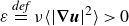 $\varepsilon \mathop {=}\limits ^{\mathit{def}} \nu \langle |\boldsymbol{\nabla } \boldsymbol{u}|^2 \rangle \gt 0$
is the rate of dissipation of kinetic energy and
$\varepsilon \mathop {=}\limits ^{\mathit{def}} \nu \langle |\boldsymbol{\nabla } \boldsymbol{u}|^2 \rangle \gt 0$
is the rate of dissipation of kinetic energy and $\langle w b \rangle$
is the rate of conversion from internal and gravitational potential energy to kinetic energy.
$\langle w b \rangle$
is the rate of conversion from internal and gravitational potential energy to kinetic energy.
Averaging the buoyancy equation (2.4) over the horizontal coordinates and time $t$
, and then integrating in
$t$
, and then integrating in $z$
, leads to the flux constraint
$z$
, leads to the flux constraint
 \begin{align} \overline {wb} - \kappa \bar b_z =\kappa \beta . \end{align}
In pure HC, with $\beta =0$
, (3.2) is the zero-flux constraint of Paparella & Young (Reference Paparella and Young2002). With non-zero buoyancy flux through the bottom, (3.2) says that in steady state the same buoyancy flux
$\beta =0$
, (3.2) is the zero-flux constraint of Paparella & Young (Reference Paparella and Young2002). With non-zero buoyancy flux through the bottom, (3.2) says that in steady state the same buoyancy flux $\kappa \beta$
must pass through every level.
$\kappa \beta$
must pass through every level.
Taking the $z$
-integral of (3.2), dividing by
$z$
-integral of (3.2), dividing by $h$
, and substituting into (3.1) gives
$h$
, and substituting into (3.1) gives
 \begin{align} \varepsilon =\kappa \beta + \kappa \langle b_z\rangle . \end{align}
In (3.3) $\varepsilon$
and
$\varepsilon$
and $\kappa \beta$
are both positive. However, the third term,
$\kappa \beta$
are both positive. However, the third term, $\kappa \langle b_z\rangle$
, might have either sign. From
$\kappa \langle b_z\rangle$
, might have either sign. From $\langle b \text{(2.4)}\rangle$
we obtain the buoyancy power integral
$\langle b \text{(2.4)}\rangle$
we obtain the buoyancy power integral
 \begin{align} \chi = \kappa \overline {b_z(h) b^{\textit{s}}(x)}/h - \kappa \beta \langle b_z \rangle , \end{align}
where $\chi \mathop {=}\limits ^{\mathit{def}} \kappa \langle |\boldsymbol{\nabla } b|^2\rangle$
is the dissipation of buoyancy variance and
$\chi \mathop {=}\limits ^{\mathit{def}} \kappa \langle |\boldsymbol{\nabla } b|^2\rangle$
is the dissipation of buoyancy variance and $b_z(h)= b_z(x,y,h,t)$
(e.g. Winters & Young Reference Winters and Young2009; Rocha et al. Reference Rocha, Constantinou, Llewellyn Smith and Young2020). Although
$b_z(h)= b_z(x,y,h,t)$
(e.g. Winters & Young Reference Winters and Young2009; Rocha et al. Reference Rocha, Constantinou, Llewellyn Smith and Young2020). Although $\chi$
is positive the terms on the right of (3.4) can have either sign.
$\chi$
is positive the terms on the right of (3.4) can have either sign.
3.2. Neutral stratification, restratification and strong restratification
In pure HC ( $F=\beta \kappa =0$
) it follows from (3.3) that
$F=\beta \kappa =0$
) it follows from (3.3) that $\langle b_z\rangle \gt 0$
. The other limiting case is pure type 3 RBC, corresponding to
$\langle b_z\rangle \gt 0$
. The other limiting case is pure type 3 RBC, corresponding to $b^{\textit{s}}(x)=0$
and
$b^{\textit{s}}(x)=0$
and $F \gt 0$
. In this case (3.4) shows that
$F \gt 0$
. In this case (3.4) shows that $\langle b_z\rangle \lt 0$
. To summarise
$\langle b_z\rangle \lt 0$
. To summarise
 \begin{align} \textit{pure HC}\, (3.3) \qquad &\Rightarrow \qquad \langle b_z \rangle \gt 0; \\[-12pt]\nonumber \end{align}
 \begin{align} \textit{pure RBC} \,(3.4) \qquad &\Rightarrow \qquad \langle b_z \rangle \lt 0. \\[10pt]\nonumber \end{align}
The results above, based on power integrals, motivate using the sign change of $\langle b_z \rangle$
to define the onset of “restratification”: we say that a bottom-heated layer with non-uniform surface temperature is restratified by HC if
$\langle b_z \rangle$
to define the onset of “restratification”: we say that a bottom-heated layer with non-uniform surface temperature is restratified by HC if $\langle b_z \rangle \gt 0$
.
$\langle b_z \rangle \gt 0$
.
At the onset of restratification, with
 \begin{align} \langle b_z\rangle = 0, \end{align}
we say that the layer has “neutral stratification”. Recalling that $\bar b(h)=0$
, the identity
$\bar b(h)=0$
, the identity
 \begin{align} \langle b_z\rangle = -\frac { \bar b(0)}{h} \end{align}
shows that a neutrally stratified layer has $\bar b(0)=0$
.
$\bar b(0)=0$
.
From the HC extremum principle (Paparella & Young Reference Paparella and Young2002), the smallest (most negative) buoyancy in the domain must be greater than the smallest buoyancy prescribed at the surface $z=h$
. Hence, for the sinusoidal surface profile in (2.6) we obtain from (3.8)
$z=h$
. Hence, for the sinusoidal surface profile in (2.6) we obtain from (3.8)
 \begin{align} \langle b_z\rangle \leqslant \frac {b_{\star }}{h} . \end{align}
Restating (3.9) in dimensionless variables produces an upper bound on the possible strength of restratification
 \begin{align} \frac {\langle b_z\rangle }{\beta } \leqslant \frac {\mathit{Ra_H}}{\mathit{Ra_V}}. \end{align}
As a definition of the situation in which HC dominates RBC we say that the layer is ‘strongly restratified’ if
 \begin{align} 1 \leqslant \frac {\langle b_z \rangle }{\beta }, \qquad \textit{(definition of strong restratification).} \end{align}
The upper bound in (3.10) shows that strong restratification is not possible if $\mathit{Ra_H}/\mathit{Ra_V} \lt 1$
.
$\mathit{Ra_H}/\mathit{Ra_V} \lt 1$
.
The bottom boundary condition is $b_z(x,y,0,t)=-\beta$
, so strong restratification means that the bulk stratification,
$b_z(x,y,0,t)=-\beta$
, so strong restratification means that the bulk stratification, $\langle b_z\rangle$
, is equal in magnitude, but opposite in sign, to the destabilising bottom buoyancy gradient. This definition of strong restratification is somewhat arbitrary. But solutions discussed in § 4 indicate that with (3.11) the top boundary layer is characteristic of HC, i.e. if inequality (3.11) applies then RBC has capitulated to HC.
$\langle b_z\rangle$
, is equal in magnitude, but opposite in sign, to the destabilising bottom buoyancy gradient. This definition of strong restratification is somewhat arbitrary. But solutions discussed in § 4 indicate that with (3.11) the top boundary layer is characteristic of HC, i.e. if inequality (3.11) applies then RBC has capitulated to HC.
Rotation does not alter the power integrals in (3.3) and (3.4). Thus the definitions of neutral and strong stratification, and all results based on power integrals, extend to rotating flows.
4. Phenomenology and the surface boundary layer
We describe the flow characteristics associated with neutral and strong restratification.
Two snapshots of the buoyancy field separated by a short time interval around $0.02\,h^2/\kappa$
for
$0.02\,h^2/\kappa$
for $(a)$
the neutral stratification state (
$(a)$
the neutral stratification state ( $\mathit{Ra_H} = 3.35\times 10^6$
) and
$\mathit{Ra_H} = 3.35\times 10^6$
) and $(b)$
the onset of the strong stratification regime (
$(b)$
the onset of the strong stratification regime ( $\mathit{Ra_H} = 2.03\times 10^7$
). Streamlines are overlaid in both cases. Parameters are
$\mathit{Ra_H} = 2.03\times 10^7$
). Streamlines are overlaid in both cases. Parameters are $\mathit{Ra_V} = 10^7$
,
$\mathit{Ra_V} = 10^7$
, $\varGamma = 8$
and
$\varGamma = 8$
and ${\textit{Pr}} = 1$
. The buoyancy unit is
${\textit{Pr}} = 1$
. The buoyancy unit is $\nu \kappa /h^3$
.
$\nu \kappa /h^3$
.

Figure 3. Long description
The heat map displays two snapshots of the buoyancy field with overlaid streamlines, illustrating the neutral stratification state and the onset of the strong stratification regime. The color scale ranges from red to blue, indicating varying buoyancy values. The neutral stratification state shows more dynamic and varied patterns, while the strong stratification state exhibits more uniform and stable patterns. The streamlines highlight the flow direction and intensity within the buoyancy fields.
4.1. Neutral stratification
In the neutrally stratified state, with $\langle b_z\rangle =0$
, rising plumes generated by the bottom buoyancy flux are intermittently swept along the bottom towards the sidewalls by a large-scale horizontal circulation, as observed in CNF. This circulation is the bottom expression of the dominant HC overturning cell, which is in turn driven by the descending plume that forms near the centre of the upper boundary. The flow alternates between RB-like convection cells and the broader HC circulation – see figure 3(a).
$\langle b_z\rangle =0$
, rising plumes generated by the bottom buoyancy flux are intermittently swept along the bottom towards the sidewalls by a large-scale horizontal circulation, as observed in CNF. This circulation is the bottom expression of the dominant HC overturning cell, which is in turn driven by the descending plume that forms near the centre of the upper boundary. The flow alternates between RB-like convection cells and the broader HC circulation – see figure 3(a).
Profiles of $\bar b(z)$
with neutral stratification are shown in figure 4(a). The buoyancy is normalised by the imposed HC surface amplitude
$\bar b(z)$
with neutral stratification are shown in figure 4(a). The buoyancy is normalised by the imposed HC surface amplitude $b_*$
, and the vertical coordinate is rescaled by the thickness of the top boundary layer
$b_*$
, and the vertical coordinate is rescaled by the thickness of the top boundary layer $\delta$
, defined as the distance from the top boundary at which
$\delta$
, defined as the distance from the top boundary at which $\bar b_z$
reaches
$\bar b_z$
reaches $95\,\%$
of its maximum value. When presented in this way,
$95\,\%$
of its maximum value. When presented in this way, $\bar b(z)$
profiles with
$\bar b(z)$
profiles with $\mathit{Ra_V} \geqslant 10^6$
collapse onto a common curve in the top boundary layer. Thus with
$\mathit{Ra_V} \geqslant 10^6$
collapse onto a common curve in the top boundary layer. Thus with $\langle b_z\rangle =0$
, the buoyancy variation across the top boundary layer is controlled by the imposed HC surface forcing
$\langle b_z\rangle =0$
, the buoyancy variation across the top boundary layer is controlled by the imposed HC surface forcing $b_{\star }$
.
$b_{\star }$
.
4.2. Strong stratification
In the strong stratification regime RBC is largely suppressed: see figures 3(b) and 4(b) in which $\langle b_z\rangle \approx + \beta$
, i.e. this is the onset of the strongly restratified regime. The horizontal bottom flow induced by the descending plumes at the top surface is sustained rather than intermittent. Some residual RBC effects remain, e.g. in figure 3(b) weak upward plumes generated by the bottom flux are visible. These small RBC bottom plumes perturb the horizontal flow and enhance mixing near the bottom boundary compared with pure HC. The structure of this flow is primarily determined by HC but retains some influence of RBC, particularly near the heated bottom and the lateral edges.
$\langle b_z\rangle \approx + \beta$
, i.e. this is the onset of the strongly restratified regime. The horizontal bottom flow induced by the descending plumes at the top surface is sustained rather than intermittent. Some residual RBC effects remain, e.g. in figure 3(b) weak upward plumes generated by the bottom flux are visible. These small RBC bottom plumes perturb the horizontal flow and enhance mixing near the bottom boundary compared with pure HC. The structure of this flow is primarily determined by HC but retains some influence of RBC, particularly near the heated bottom and the lateral edges.
Vertical profile of the horizontally averaged buoyancy for several $\mathit{Ra_V}$
, normalised by
$\mathit{Ra_V}$
, normalised by $b_{\star }$
in the neutral stratification regime in
$b_{\star }$
in the neutral stratification regime in $(a)$
and by
$(a)$
and by $\beta h$
in the strong stratification regime in
$\beta h$
in the strong stratification regime in $(b)$
. The boundary-layer thickness
$(b)$
. The boundary-layer thickness $\delta$
is computed from the vertical profile of
$\delta$
is computed from the vertical profile of $\bar b_z(z)$
by determining the depth at which
$\bar b_z(z)$
by determining the depth at which $95\,\%$
of the maximum value of
$95\,\%$
of the maximum value of $\bar b_z$
is reached. The parameters are
$\bar b_z$
is reached. The parameters are $\varGamma = 8$
and
$\varGamma = 8$
and ${\textit{Pr}}=1$
.
${\textit{Pr}}=1$
.

Figure 4. Long description
Two line graphs depict the vertical profile of horizontally averaged buoyancy in different stratification regimes. The left graph shows the neutral stratification regime, while the right graph shows the strong stratification regime. Each graph includes multiple lines representing different Rayleigh numbers (RaV) of 10^5, 10^6, 10^7, and 10^8. The x-axis represents normalized buoyancy, and the y-axis represents the normalized height. The boundary-layer thickness is computed from the vertical profile by determining the depth at which a fraction of the maximum value of buoyancy is reached. The parameters used are specific to each regime. The graphs illustrate how buoyancy varies with height under different conditions of geothermal heating and ice sheet thickness, highlighting the impact of horizontal non-uniformities in basal ice temperature, heat flux, salinity fluxes, and water layer depth.
Vertical profiles of the horizontally averaged buoyancy $\bar b(z)$
for several values of
$\bar b(z)$
for several values of $\mathit{Ra_V}$
are shown in figure 4(b). The buoyancy is normalised by the bottom forcing scale
$\mathit{Ra_V}$
are shown in figure 4(b). The buoyancy is normalised by the bottom forcing scale $\beta h$
. As in the neutral case, the vertical coordinate is rescaled by the thickness of the top boundary layer
$\beta h$
. As in the neutral case, the vertical coordinate is rescaled by the thickness of the top boundary layer $\delta$
, defined as the depth at which
$\delta$
, defined as the depth at which $\bar b_z$
reaches
$\bar b_z$
reaches $95\,\%$
of its maximum value.
$95\,\%$
of its maximum value.
In this strongly restratified regime, with $\langle b_z \rangle \approx +\beta$
, the horizontally averaged buoyancy at the bottom is
$\langle b_z \rangle \approx +\beta$
, the horizontally averaged buoyancy at the bottom is $\bar b(0) = -\beta h$
. When normalised by
$\bar b(0) = -\beta h$
. When normalised by $\beta h$
, the
$\beta h$
, the $\bar b(z)$
profiles collapse near the top boundary – see figure 4(b) – indicating that the buoyancy variation across the top boundary layer is now controlled by
$\bar b(z)$
profiles collapse near the top boundary – see figure 4(b) – indicating that the buoyancy variation across the top boundary layer is now controlled by $\beta$
and confirming that this normalisation of
$\beta$
and confirming that this normalisation of $\bar b$
captures the structure of the top boundary layer at the onset of the strongly restratified state.
$\bar b$
captures the structure of the top boundary layer at the onset of the strongly restratified state.
4.3. Transition Rayleigh numbers
Consider a flow forced with a fixed value of $\mathit{Ra_V}$
. If
$\mathit{Ra_V}$
. If $\mathit{Ra_H}=0$
(pure RBC), then from (3.4)
$\mathit{Ra_H}=0$
(pure RBC), then from (3.4) $\langle b_z\rangle \lt 0$
. As
$\langle b_z\rangle \lt 0$
. As $\mathit{Ra_H}$
is increased from zero, the flow initially remains unchanged and continues to be dominated by RBC. With further increases in
$\mathit{Ra_H}$
is increased from zero, the flow initially remains unchanged and continues to be dominated by RBC. With further increases in $\mathit{Ra_H}$
the system undergoes a sharp transition: the convection pattern alternates between RBC cells and a large horizontal circulation driven by intermittent descending plumes from the upper boundary. This transition corresponds to the regime change identified and discussed by CNF. Further increasing
$\mathit{Ra_H}$
the system undergoes a sharp transition: the convection pattern alternates between RBC cells and a large horizontal circulation driven by intermittent descending plumes from the upper boundary. This transition corresponds to the regime change identified and discussed by CNF. Further increasing $\mathit{Ra_H}$
raises
$\mathit{Ra_H}$
raises $\langle b_z\rangle$
, and at some HC Rayleigh number, denoted
$\langle b_z\rangle$
, and at some HC Rayleigh number, denoted $\mathit{Ra}^{\mathit{N}}_{\mathit{H}}$
, the flow is neutrally stratified with
$\mathit{Ra}^{\mathit{N}}_{\mathit{H}}$
, the flow is neutrally stratified with $\langle b_z\rangle =0$
. With further increase in
$\langle b_z\rangle =0$
. With further increase in $\mathit{Ra_H}$
the flow becomes strongly restratified at
$\mathit{Ra_H}$
the flow becomes strongly restratified at $\mathit{Ra}^{\mathit{S}}_{\mathit{H}} \gt \mathit{Ra}^{\mathit{N}}_{\mathit{H}}$
. To precisely characterise these transitions we define the horizontal Rayleigh numbers corresponding to the neutral and strong stratification states respectively as
$\mathit{Ra}^{\mathit{S}}_{\mathit{H}} \gt \mathit{Ra}^{\mathit{N}}_{\mathit{H}}$
. To precisely characterise these transitions we define the horizontal Rayleigh numbers corresponding to the neutral and strong stratification states respectively as
 \begin{align} &\mathit{Ra}^{\mathit{N}}_{\mathit{H}}(\mathit{Ra_V},\varGamma ,{\textit{Pr}}): \quad \mathit{Ra_H} \ \textrm{at which} \ \langle b_z \rangle = 0, \\[-12pt] \nonumber \end{align}
 \begin{align} &\mathit{Ra}^{\mathit{S}}_{\mathit{H}}(\mathit{Ra_V},\varGamma ,{\textit{Pr}}): \quad \mathit{Ra_H} \ \textrm{at which} \ \langle b_z \rangle = \beta . \\[10pt] \nonumber \end{align}
Figure 5 shows the functions $\mathit{Ra}^{\mathit{N}}_{\mathit{H}}$
and
$\mathit{Ra}^{\mathit{N}}_{\mathit{H}}$
and $\mathit{Ra}^{\mathit{S}}_{\mathit{H}}$
in the
$\mathit{Ra}^{\mathit{S}}_{\mathit{H}}$
in the $(\mathit{Ra_H},\mathit{Ra_V})$
parameter space for
$(\mathit{Ra_H},\mathit{Ra_V})$
parameter space for ${\textit{Pr}}=1$
; we consider several aspect ratios as indicated. Each point in figure 5 is determined using a bisection search: to determine
${\textit{Pr}}=1$
; we consider several aspect ratios as indicated. Each point in figure 5 is determined using a bisection search: to determine $\mathit{Ra}^{\mathit{N}}_{\mathit{H}}$
we fix
$\mathit{Ra}^{\mathit{N}}_{\mathit{H}}$
we fix $\mathit{Ra_V}$
,
$\mathit{Ra_V}$
, $\varGamma$
and
$\varGamma$
and ${\textit{Pr}}$
. We then obtain a sequence of solutions in which the target
${\textit{Pr}}$
. We then obtain a sequence of solutions in which the target $\mathit{Ra}^{\mathit{N}}_{\mathit{H}}$
is bracketed and repeatedly halved until we located the value of
$\mathit{Ra}^{\mathit{N}}_{\mathit{H}}$
is bracketed and repeatedly halved until we located the value of $\mathit{Ra_H}$
for which
$\mathit{Ra_H}$
for which $|\langle b_z\rangle /\beta |\leq 0.05$
. The shaded regions in figure 5 indicate the uncertainty.
$|\langle b_z\rangle /\beta |\leq 0.05$
. The shaded regions in figure 5 indicate the uncertainty. $(a)$
Neutral horizontal Rayleigh number
$(a)$
Neutral horizontal Rayleigh number $\mathit{Ra}^{\mathit{N}}_{\mathit{H}}$
(defined as the value of
$\mathit{Ra}^{\mathit{N}}_{\mathit{H}}$
(defined as the value of $\mathit{Ra_H}$
for which
$\mathit{Ra_H}$
for which $\langle b_z \rangle = 0$
at a given
$\langle b_z \rangle = 0$
at a given $\mathit{Ra_V}$
) plotted as a function of
$\mathit{Ra_V}$
) plotted as a function of $\mathit{Ra_V}$
for several aspect ratios. The inset shows the same data compensated by the scaling law (5.10), For the two last
$\mathit{Ra_V}$
for several aspect ratios. The inset shows the same data compensated by the scaling law (5.10), For the two last $\mathit{Ra_V}$
values (
$\mathit{Ra_V}$
values ( $10^9$
,
$10^9$
, $10^{10}$
), data are shown only for
$10^{10}$
), data are shown only for $\varGamma =8$
.
$\varGamma =8$
. $(b)$
Strong horizontal Rayleigh number
$(b)$
Strong horizontal Rayleigh number $\mathit{Ra}^{\mathit{S}}_{\mathit{H}}$
(defined as the value of
$\mathit{Ra}^{\mathit{S}}_{\mathit{H}}$
(defined as the value of $\mathit{Ra_H}$
for which
$\mathit{Ra_H}$
for which $\langle b_z \rangle = \beta$
at a given
$\langle b_z \rangle = \beta$
at a given $\mathit{Ra_V}$
) plotted as a function of
$\mathit{Ra_V}$
) plotted as a function of $\mathit{Ra_V}$
for several aspect ratios. The inset shows the same data compensated by the scaling law (5.14). For the last
$\mathit{Ra_V}$
for several aspect ratios. The inset shows the same data compensated by the scaling law (5.14). For the last $\mathit{Ra_V}$
value (
$\mathit{Ra_V}$
value ( $10^9$
), data are shown only for
$10^9$
), data are shown only for $\varGamma =8$
. Empty/full symbols indicate respectively filtered/direct numerical simulations.
$\varGamma =8$
. Empty/full symbols indicate respectively filtered/direct numerical simulations.

Figure 5. Long description
The image contains two graphs. The first graph on the left shows the neutral horizontal Rayleigh number as a function of the Rayleigh number for several aspect ratios. The data points are represented by different colored symbols corresponding to different aspect ratios. The inset within this graph shows the same data compensated by a specific scaling law. For the two highest values of the Rayleigh number, data are shown only for a specific range. The second graph on the right illustrates the strong horizontal Rayleigh number as a function of the Rayleigh number for several aspect ratios. Similar to the first graph, the inset shows the same data compensated by a different scaling law. For the highest value of the Rayleigh number, data are shown only for a specific range. Empty and full symbols indicate filtered and direct numerical simulations, respectively.
For low Rayleigh numbers ( $\mathit{Ra_H}, \mathit{Ra_V} \lesssim 10^4$
), both neutral stratification and the onset of the strong stratification regime follow a power-law scaling
$\mathit{Ra_H}, \mathit{Ra_V} \lesssim 10^4$
), both neutral stratification and the onset of the strong stratification regime follow a power-law scaling
 \begin{align} \left(\mathit{Ra}^{\mathit{N}}_{\mathit{H}},\mathit{Ra}^{\mathit{S}}_{\mathit{H}}\right)\sim \mathit{Ra_V}^{1/2} \varGamma \end{align}
with no dependence on ${\textit{Pr}}$
. Thus a main conclusion is that the neutral curve
${\textit{Pr}}$
. Thus a main conclusion is that the neutral curve $\mathit{Ra_H}=\mathit{Ra}^{\mathit{N}}_{\mathit{H}}(\mathit{Ra_V},\varGamma ,{\textit{Pr}})$
passes through the origin of the
$\mathit{Ra_H}=\mathit{Ra}^{\mathit{N}}_{\mathit{H}}(\mathit{Ra_V},\varGamma ,{\textit{Pr}})$
passes through the origin of the $(\mathit{Ra_V},\mathit{Ra_H})$
parameter plane. Further detail and an analytic explanation of (4.3) are in Appendix C.
$(\mathit{Ra_V},\mathit{Ra_H})$
parameter plane. Further detail and an analytic explanation of (4.3) are in Appendix C.
At higher Rayleigh numbers ( $\mathit{Ra_H}, \mathit{Ra_V} \gtrsim 10^4$
), the system enters an aspect-ratio-independent regime, with
$\mathit{Ra_H}, \mathit{Ra_V} \gtrsim 10^4$
), the system enters an aspect-ratio-independent regime, with
 \begin{align} \mathit{Ra}^{\mathit{N}}_{\mathit{H}}(\mathit{Ra_V},\varGamma ,1) \sim 8.54\,\mathit{Ra_V}^{4/5}. \end{align}
The onset of the strong stratification regime is at
 \begin{align} \mathit{Ra}^{\mathit{S}}_{\mathit{H}}(\mathit{Ra_V},\varGamma ,1) \sim 1.70\,\mathit{Ra_V} . \end{align}
The scaling above is consistent with the conclusion following (3.11) that strong restratification requires $\mathit{Ra_H}\gt \mathit{Ra_V}$
.
$\mathit{Ra_H}\gt \mathit{Ra_V}$
.
The regimes in (4.4) and (4.5) are independent of aspect ratio $\varGamma$
. This underscores the relevance of the layer thickness
$\varGamma$
. This underscores the relevance of the layer thickness $h$
as the characteristic length scale of the system and motivates the definition of
$h$
as the characteristic length scale of the system and motivates the definition of $\mathit{Ra_H}$
in (2.7) – using
$\mathit{Ra_H}$
in (2.7) – using $\mathit{Ra^{trad}_H}$
in (2.9) introduces an artificial dependence on
$\mathit{Ra^{trad}_H}$
in (2.9) introduces an artificial dependence on $\varGamma$
. Figures 5(a) and 5(b) show our estimates of
$\varGamma$
. Figures 5(a) and 5(b) show our estimates of $\mathit{Ra}^{\mathit{N}}_{\mathit{H}}$
and
$\mathit{Ra}^{\mathit{N}}_{\mathit{H}}$
and $\mathit{Ra}^{\mathit{S}}_{\mathit{H}}$
at
$\mathit{Ra}^{\mathit{S}}_{\mathit{H}}$
at ${\textit{Pr}}=1$
for different values of the aspect ratio
${\textit{Pr}}=1$
for different values of the aspect ratio $\varGamma$
.
$\varGamma$
.
5. Scaling analysis
In this section, we analyse the system using scaling arguments, focusing on regimes where either RBC or HC dominates, as well as the neutral state with $\langle b_z \rangle =0$
and the onset of strong stratification at
$\langle b_z \rangle =0$
and the onset of strong stratification at $\langle b_z \rangle =+\beta$
. The horizontallyaveraged buoyancy equation (3.2) shows that the buoyancy flux entering the domain through the bottom boundary layer must be conserved across any horizontal plane. Consequently, buoyancy must be extracted through a boundary layer at the top surface, leading to
$\langle b_z \rangle =+\beta$
. The horizontallyaveraged buoyancy equation (3.2) shows that the buoyancy flux entering the domain through the bottom boundary layer must be conserved across any horizontal plane. Consequently, buoyancy must be extracted through a boundary layer at the top surface, leading to $\bar {b}_z(h) = -\beta$
. Due to the imposed buoyancy profile at the top boundary, we expect this upper region to be the primary site where the competition between RBC and HC manifests itself, thereby governing the global dynamics of the system. We therefore focus on the structure and behaviour of the top boundary layer.
$\bar {b}_z(h) = -\beta$
. Due to the imposed buoyancy profile at the top boundary, we expect this upper region to be the primary site where the competition between RBC and HC manifests itself, thereby governing the global dynamics of the system. We therefore focus on the structure and behaviour of the top boundary layer.
Most of our numerical solutions use ${\textit{Pr}}=1$
and we do not distinguish between viscous and buoyancy boundary layers. We assume that the characteristic vertical length scale is given by the thickness of the top boundary layer, denoted by
${\textit{Pr}}=1$
and we do not distinguish between viscous and buoyancy boundary layers. We assume that the characteristic vertical length scale is given by the thickness of the top boundary layer, denoted by $\delta$
, such that
$\delta$
, such that $\partial /\partial _z \sim 1/\delta$
. The characteristic horizontal length scale is taken to be
$\partial /\partial _z \sim 1/\delta$
. The characteristic horizontal length scale is taken to be $\ell$
, which will be specified for each regime considered, implying
$\ell$
, which will be specified for each regime considered, implying $\partial /\partial _x \sim 1/\ell$
.
$\partial /\partial _x \sim 1/\ell$
.
We expect that a significant portion of both viscous and buoyancy dissipation is concentrated within the boundary layers (BLs), which occupy a fraction $\delta /h$
of the domain. Accordingly, we estimate the dissipation rates as
$\delta /h$
of the domain. Accordingly, we estimate the dissipation rates as
 \begin{equation} \varepsilon = \nu \langle |\boldsymbol{\nabla }\boldsymbol{u}|^2 \rangle \sim \nu \frac {U^2}{\delta ^2} \left ( \frac {\delta }{h} \right )\!, \quad \chi = \kappa \langle |\boldsymbol{\nabla }b|^2 \rangle \sim \kappa \frac {B^2}{\delta ^2} \left ( \frac {\delta }{h} \right )\!, \end{equation}
where $U$
is the characteristic horizontal velocity and
$U$
is the characteristic horizontal velocity and $B$
is the buoyancy difference across the top BL, with the factor
$B$
is the buoyancy difference across the top BL, with the factor $(\delta /h)$
coming from the ratio of the BL thickness to the total depth.
$(\delta /h)$
coming from the ratio of the BL thickness to the total depth.
From mass conservation (2.5), we obtain the relation $U/\ell \sim W/\delta$
, where
$U/\ell \sim W/\delta$
, where $W$
is the characteristic vertical velocity within the top BL. Balancing advection with diffusion in the buoyancy equation (2.4) and this relation yields a scaling for the horizontal velocity
$W$
is the characteristic vertical velocity within the top BL. Balancing advection with diffusion in the buoyancy equation (2.4) and this relation yields a scaling for the horizontal velocity
 \begin{equation} U \sim \frac {\kappa \ell }{\delta ^2}. \end{equation}
5.1. Scalings in the asymptotic regimes
We now derive scaling laws for the top BL thickness and mean buoyancy in two asymptotic regimes: when RBC dominates HC ( $\mathit{Ra_V} \gg \mathit{Ra_H}$
), and when HC dominates RBC (
$\mathit{Ra_V} \gg \mathit{Ra_H}$
), and when HC dominates RBC ( $\mathit{Ra_H} \gg \mathit{Ra_V}$
).
$\mathit{Ra_H} \gg \mathit{Ra_V}$
).
Vertical profiles of the mean vertical buoyancy gradient, $\bar {b}_z$
, for varying
$\bar {b}_z$
, for varying $\mathit{Ra_V}$
with fixed
$\mathit{Ra_V}$
with fixed $\mathit{Ra_H} = 10^2$
in panel
$\mathit{Ra_H} = 10^2$
in panel $(a)$
. Dash–dot lines indicate the estimated thickness of the top BL. Insets show snapshots of the buoyancy field: in
$(a)$
. Dash–dot lines indicate the estimated thickness of the top BL. Insets show snapshots of the buoyancy field: in $(a)$
, for pure RBC (top,
$(a)$
, for pure RBC (top, $\mathit{Ra_V} = 10^8$
) and a mixed case (bottom,
$\mathit{Ra_V} = 10^8$
) and a mixed case (bottom, $\mathit{Ra_V} = 10^8$
,
$\mathit{Ra_V} = 10^8$
, $\mathit{Ra_H} = 10^2$
). Panel
$\mathit{Ra_H} = 10^2$
). Panel $(b)$
shows the BL thickness
$(b)$
shows the BL thickness $\delta$
as a function of
$\delta$
as a function of $\mathit{Ra_V}$
for both pure RBC and mixed case. Panel
$\mathit{Ra_V}$
for both pure RBC and mixed case. Panel $(c)$
shows the norm of the mean vertical buoyancy gradient,
$(c)$
shows the norm of the mean vertical buoyancy gradient, $|\langle b_z \rangle |$
, and its dependence on
$|\langle b_z \rangle |$
, and its dependence on $\mathit{Ra_V}$
for both pure RBC and mixed cases.
$\mathit{Ra_V}$
for both pure RBC and mixed cases.

Figure 6. Long description
The image contains three graphs. The first graph on the left shows vertical profiles of the mean vertical buoyancy gradient for varying Rayleigh numbers with a fixed horizontal Rayleigh number. Different colored lines represent different Rayleigh numbers, and dash-dot lines indicate the estimated thickness of the top boundary layer. Insets within this graph display snapshots of the buoyancy field for pure Rayleigh-Bénard convection and a mixed case. The second graph on the top right illustrates the boundary layer thickness as a function of the vertical Rayleigh number for both pure Rayleigh-Bénard convection and the mixed case, with a dashed line showing a power-law relationship. The third graph on the bottom right presents the norm of the mean vertical buoyancy gradient and its dependence on the vertical Rayleigh number for both pure Rayleigh-Bénard convection and mixed cases, also with a dashed line indicating a power-law relationship. All values are approximated.
5.1.1. The RBC-dominated regime
When the flux Rayleigh number greatly exceeds the horizontal Rayleigh number ( $\mathit{Ra_V} \gg \mathit{Ra_H}$
), the dynamics is controlled by RBC. The horizontal length scale is set by the depth of the layer,
$\mathit{Ra_V} \gg \mathit{Ra_H}$
), the dynamics is controlled by RBC. The horizontal length scale is set by the depth of the layer, $\ell \sim h$
, and the imposed bottom buoyancy flux dominates the surface forcing. In this limit the power integrals (3.3)–(3.4) reduce to
$\ell \sim h$
, and the imposed bottom buoyancy flux dominates the surface forcing. In this limit the power integrals (3.3)–(3.4) reduce to
 \begin{equation} \varepsilon \approx \kappa \beta \quad \textrm{and} \quad \chi \approx -\kappa \beta \langle b_z \rangle . \end{equation}
Assuming $\langle b_z \rangle \sim B/h$
, i.e.
$\langle b_z \rangle \sim B/h$
, i.e. $(B /\delta )$
times the global average factor
$(B /\delta )$
times the global average factor $(\delta /h)$
and substituting the dissipation scalings (5.1) into (5.3) yields
$(\delta /h)$
and substituting the dissipation scalings (5.1) into (5.3) yields
 \begin{equation} \delta \sim h \mathit{Ra_V}^{-1/5}, \quad B \sim \beta \delta \sim \beta h \mathit{Ra_V}^{-1/5}. \end{equation}
These scalings are the fixed-flux equivalent of the regime-I scalings of Grossmann & Lohse (Reference Grossmann and Lohse2000) for fixed-temperature boundaries, namely $\delta \sim h Ra_{\Delta b}^{-1/4}$
, where
$\delta \sim h Ra_{\Delta b}^{-1/4}$
, where $Ra_{\Delta b}$
is the classical RBC parameter based on the buoyancy difference
$Ra_{\Delta b}$
is the classical RBC parameter based on the buoyancy difference $\Delta b$
between the top and bottom plate. Adapting
$\Delta b$
between the top and bottom plate. Adapting $Ra_{\Delta b}^{-1/4}$
to an an imposed bottom flux using
$Ra_{\Delta b}^{-1/4}$
to an an imposed bottom flux using $\Delta b \approx \beta \delta$
gives
$\Delta b \approx \beta \delta$
gives $Ra_{\Delta b} = (\delta /h)\mathit{Ra_V}$
(Otero et al. Reference Otero, Wittengerb, Worthing and Doering2002; Johnston & Doering Reference Johnston and Doering2009), which then recovers (5.4) for the BL thickness.
$Ra_{\Delta b} = (\delta /h)\mathit{Ra_V}$
(Otero et al. Reference Otero, Wittengerb, Worthing and Doering2002; Johnston & Doering Reference Johnston and Doering2009), which then recovers (5.4) for the BL thickness.
The predicted trends are confirmed in figures 6(b) and 6(c). Profiles of $\bar b_z$
(panel a) show the definition of the top BL thickness
$\bar b_z$
(panel a) show the definition of the top BL thickness $\delta$
, taken as the distance from the top where
$\delta$
, taken as the distance from the top where $\bar b_z$
falls to
$\bar b_z$
falls to $95\,\%$
of its maximum. In these panels, we present data from pure RBC simulations at
$95\,\%$
of its maximum. In these panels, we present data from pure RBC simulations at $\mathit{Ra_V} = 10^8$
and from a mixed-forcing case with
$\mathit{Ra_V} = 10^8$
and from a mixed-forcing case with $\mathit{Ra_V} = 10^8$
and
$\mathit{Ra_V} = 10^8$
and $\mathit{Ra_H} = 10^2$
. For the mixed case with
$\mathit{Ra_H} = 10^2$
. For the mixed case with $\mathit{Ra_V}=10^8$
and
$\mathit{Ra_V}=10^8$
and $\mathit{Ra_H}=10^2$
, the data for both
$\mathit{Ra_H}=10^2$
, the data for both $\delta$
and
$\delta$
and $|\langle b_z \rangle |$
collapse onto those from pure RBC, indicating that the dynamics remains governed by RBC, with the horizontal forcing being too weak to produce any significant modification (see inset in figure 6(a)).
$|\langle b_z \rangle |$
collapse onto those from pure RBC, indicating that the dynamics remains governed by RBC, with the horizontal forcing being too weak to produce any significant modification (see inset in figure 6(a)).
5.1.2. The HC-dominated regime
Vertical profiles of the mean vertical buoyancy gradient, $\bar {b}_z$
, for varying
$\bar {b}_z$
, for varying $\mathit{Ra_H}$
with fixed
$\mathit{Ra_H}$
with fixed $\mathit{Ra_V} = 10^2$
in panel
$\mathit{Ra_V} = 10^2$
in panel $(a)$
. Dash–dot lines indicate the estimated thickness of the top BL. Insets show snapshots of the buoyancy field for pure HC (top,
$(a)$
. Dash–dot lines indicate the estimated thickness of the top BL. Insets show snapshots of the buoyancy field for pure HC (top, $\mathit{Ra_H} = 10^8$
) and a mixed regime (bottom,
$\mathit{Ra_H} = 10^8$
) and a mixed regime (bottom, $\mathit{Ra_H} = 10^8$
,
$\mathit{Ra_H} = 10^8$
, $\mathit{Ra_V} = 10^2$
). Panel
$\mathit{Ra_V} = 10^2$
). Panel $(b)$
shows the BL thickness
$(b)$
shows the BL thickness $\delta$
as a function of
$\delta$
as a function of $\mathit{Ra_H}$
for both pure HC and mixed regime. Panel
$\mathit{Ra_H}$
for both pure HC and mixed regime. Panel $(c)$
shows the mean vertical buoyancy gradient
$(c)$
shows the mean vertical buoyancy gradient $\langle b_z \rangle$
, and its dependence in
$\langle b_z \rangle$
, and its dependence in $\mathit{Ra_H}$
for both pure HC and mixed regimes.
$\mathit{Ra_H}$
for both pure HC and mixed regimes.

Figure 7. Long description
The image contains three graphs. The first graph shows vertical profiles of the mean vertical buoyancy gradient for varying Rayleigh numbers with a fixed parameter. Dashdot lines indicate the estimated thickness of the top boundary layer. Insets display snapshots of the buoyancy field for pure horizontal convection and a mixed regime. The second graph illustrates the boundary layer thickness as a function of Rayleigh number for both pure horizontal convection and mixed regime. The third graph presents the mean vertical buoyancy gradient and its dependence on Rayleigh number for both pure horizontal convection and mixed regimes. All values are approximated.
When the horizontal Rayleigh number is much larger than the flux Rayleigh number ( $\mathit{Ra_H} \gg \mathit{Ra_V}$
), the flow is governed by HC. The relevant horizontal scale is that of the imposed surface buoyancy profile,
$\mathit{Ra_H} \gg \mathit{Ra_V}$
), the flow is governed by HC. The relevant horizontal scale is that of the imposed surface buoyancy profile, $\ell \sim \ell _x$
, and the surface forcing overwhelms the bottom flux. In this limit the power integrals reduce to
$\ell \sim \ell _x$
, and the surface forcing overwhelms the bottom flux. In this limit the power integrals reduce to
 \begin{equation} \varepsilon \approx \kappa \langle b_z \rangle , \qquad \chi \approx \frac {\kappa }{h}\,\overline {b_z(h)\,b^{\textit{s}}(x)} . \end{equation}
Using the dissipation estimates (5.1) gives
 \begin{equation} \delta \sim \ell _x \big ( \mathit{Ra_H} \varGamma ^3 \big )^{-1/5}, \qquad B \sim b_{\star } \sim \frac {\nu \kappa }{h^3}\,\mathit{Ra_H} . \end{equation}
The explicit dependence on aspect ratio $\varGamma$
reflects the fact that the HC Rayleigh number is naturally defined with the horizontal scale,
$\varGamma$
reflects the fact that the HC Rayleigh number is naturally defined with the horizontal scale, $Ra_{\ell _x} = \mathit{Ra_H} \varGamma ^3$
. These scalings coincide with the classical HC results of Rossby (Reference Rossby1965); see also the review of Hughes & Griffiths (Reference Hughes and Griffiths2008).
$Ra_{\ell _x} = \mathit{Ra_H} \varGamma ^3$
. These scalings coincide with the classical HC results of Rossby (Reference Rossby1965); see also the review of Hughes & Griffiths (Reference Hughes and Griffiths2008).
The agreement with numerical solutions is shown in figures 7(b) and 7(c). In these panels, we show data from pure HC simulations at $\mathit{Ra_H} = 10^8$
and from a mixed-forcing case with
$\mathit{Ra_H} = 10^8$
and from a mixed-forcing case with $\mathit{Ra_H} = 10^8$
and
$\mathit{Ra_H} = 10^8$
and $\mathit{Ra_V} = 10^2$
. For the mixed case, the measured
$\mathit{Ra_V} = 10^2$
. For the mixed case, the measured $\delta$
and
$\delta$
and $|\langle b_z \rangle |$
collapse onto those from pure HC, indicating that the weak bottom forcing produces no measurable departure from HC behaviour (see inset of figure 7(a)).
$|\langle b_z \rangle |$
collapse onto those from pure HC, indicating that the weak bottom forcing produces no measurable departure from HC behaviour (see inset of figure 7(a)).
5.2. Neutral stratification state
Having examined the asymptotic regimes dominated by either RBC or HC, we now turn to the intermediate case corresponding to neutral stratification, defined by $\langle b_z \rangle = 0$
. We adopt the same scaling approach as in the asymptotic regimes. In this transitional state, where neither forcing clearly dominates, the characteristic horizontal length scale is expected to scale with the domain height, i.e.
$\langle b_z \rangle = 0$
. We adopt the same scaling approach as in the asymptotic regimes. In this transitional state, where neither forcing clearly dominates, the characteristic horizontal length scale is expected to scale with the domain height, i.e. $\ell \sim h$
. Importantly, with the condition
$\ell \sim h$
. Importantly, with the condition $\langle b_z \rangle = 0$
, the power integrals (3.3) and (3.4) simplify to two-term expressions
$\langle b_z \rangle = 0$
, the power integrals (3.3) and (3.4) simplify to two-term expressions
 \begin{equation} \varepsilon = \kappa \beta \quad \textrm{and} \quad \chi = \frac {\kappa }{h} \, \overline {b_z(h) \, b^{\textit{s}}(x)}. \end{equation}
Reflecting the mixed nature of the neutral stratification state, $\varepsilon$
has the same expression as in the RBC-dominated regime (5.3), while
$\varepsilon$
has the same expression as in the RBC-dominated regime (5.3), while $\chi$
has the HC- form in (5.5). Substituting the dissipation scalings from (5.1) into (5.7) yields the following relations for the top BL thickness and buoyancy jump
$\chi$
has the HC- form in (5.5). Substituting the dissipation scalings from (5.1) into (5.7) yields the following relations for the top BL thickness and buoyancy jump
 \begin{equation} \delta \sim h \mathit{Ra_V}^{-1/5}, \quad B \sim b_{\star } \sim \frac {\nu \kappa }{h^3} \mathit{Ra_H}. \end{equation}
Thus, the BL thickness follows the RBC scaling, while the buoyancy difference across the BL follows the HC scaling. Moreover the scaling for the buoyancy jump is consistent with figure 4(a). However, since the net buoyancy flux must exit through the top BL, the horizontally averaged buoyancy equation (3.2) still imposes the condition $\bar {b}_z \approx -\beta$
. Using this, along with the scaling
$\bar {b}_z \approx -\beta$
. Using this, along with the scaling $\bar {b}_z \sim b_{\star }/\delta$
, we obtain
$\bar {b}_z \sim b_{\star }/\delta$
, we obtain
 \begin{equation} b_{\star } \sim \beta \delta . \end{equation}
Multiplying both sides of (5.9) by $h^4 / (\nu \kappa )$
and substituting the expression for
$h^4 / (\nu \kappa )$
and substituting the expression for $\delta$
from (5.8) leads to the following relation:
$\delta$
from (5.8) leads to the following relation:
 \begin{equation} \mathit{Ra}^{\mathit{N}}_{\mathit{H}} \sim \mathit{Ra_V}^{4/5}. \end{equation}
This scaling is in excellent agreement with the transition identified in figure 5(a), thereby confirming the theoretical prediction.
5.3. The onset of strong stratification
We now consider the onset of the strong stratification, defined by the condition that $\langle b_z \rangle = +\beta$
, i.e. the global stratification is equal in magnitude, but opposite in sign, to
$\langle b_z \rangle = +\beta$
, i.e. the global stratification is equal in magnitude, but opposite in sign, to $\bar b_z$
at the top and bottom of the layer. In this regime, HC is expected to dominate the dynamics, although not fully, meaning the characteristic horizontal length scale remains set by the domain height,
$\bar b_z$
at the top and bottom of the layer. In this regime, HC is expected to dominate the dynamics, although not fully, meaning the characteristic horizontal length scale remains set by the domain height, $\ell \sim h$
, rather than the imposed surface scale
$\ell \sim h$
, rather than the imposed surface scale $\ell _x$
(see figure 3).
$\ell _x$
(see figure 3).
With $\langle b_z \rangle = +\beta$
the power integrals (3.3) and (3.4) simplify to
$\langle b_z \rangle = +\beta$
the power integrals (3.3) and (3.4) simplify to
 \begin{equation} \varepsilon = 2\kappa \beta , \quad \textrm{and} \quad \chi = \frac {\kappa }{h} \, \overline {b_z(h) \, b^{\textit{s}}(x)} - \kappa \beta ^2. \end{equation}
As in the neutral regime, $\varepsilon$
follows the RBC scaling (5.3), while the buoyancy variance dissipation
$\varepsilon$
follows the RBC scaling (5.3), while the buoyancy variance dissipation $\chi$
includes contributions from both RBC and HC. Substituting the dissipation scalings from (5.1) into (5.11) yields the following expressions for the top BL thickness and buoyancy jump:
$\chi$
includes contributions from both RBC and HC. Substituting the dissipation scalings from (5.1) into (5.11) yields the following expressions for the top BL thickness and buoyancy jump:
 \begin{equation} \delta \sim h \mathit{Ra_V}^{-1/5}, \quad B \sim b_{\star } - \frac {\beta ^2 \delta h}{B}. \end{equation}
The BL thickness continues to follow the RBC scaling in (5.8), while the buoyancy jump $B$
is modified by a combination of HC and RBC effects. Because
$B$
is modified by a combination of HC and RBC effects. Because $\langle b_z\rangle =\beta$
and
$\langle b_z\rangle =\beta$
and $\langle b_z\rangle \sim B/h$
, it follows that
$\langle b_z\rangle \sim B/h$
, it follows that $B \sim \beta h$
, in agreement with the scaling shown in figure 4(b). Substituting
$B \sim \beta h$
, in agreement with the scaling shown in figure 4(b). Substituting $B \sim \beta h$
into the expression for
$B \sim \beta h$
into the expression for $B$
in (5.12) leads to
$B$
in (5.12) leads to
 \begin{equation} b_{\star } \sim \beta h \left (1 + \frac {\delta }{h} \right )\!. \end{equation}
Multiplying both sides of (5.13) by $h^3 / (\nu \kappa )$
and using the RBC scaling for
$h^3 / (\nu \kappa )$
and using the RBC scaling for $\delta$
from (5.8), we obtain the following scaling:
$\delta$
from (5.8), we obtain the following scaling:
 \begin{equation} \mathit{Ra}^{\mathit{S}}_{\mathit{H}} \sim \mathit{Ra_V} \big (1 + \mathit{Ra_V}^{-1/5} \big ). \end{equation}
The relation above reveals two distinct contributions to $\mathit{Ra}^{\mathit{S}}_{\mathit{H}}$
: a dominant term proportional to
$\mathit{Ra}^{\mathit{S}}_{\mathit{H}}$
: a dominant term proportional to $\mathit{Ra_V}$
and a correction scaling with
$\mathit{Ra_V}$
and a correction scaling with $\mathit{Ra_V}^{4/5}$
. In the asymptotic limit
$\mathit{Ra_V}^{4/5}$
. In the asymptotic limit $\mathit{Ra_V} \gg 1$
, the leading-order behaviour is
$\mathit{Ra_V} \gg 1$
, the leading-order behaviour is $\mathit{Ra}^{\mathit{S}}_{\mathit{H}} \sim \mathit{Ra_V}$
. This scaling is in agreement with the transition identified in figure 5(b).
$\mathit{Ra}^{\mathit{S}}_{\mathit{H}} \sim \mathit{Ra_V}$
. This scaling is in agreement with the transition identified in figure 5(b).
The scaling arguments above apply to the regime in which the flow remains BL dominated (regime-I of Grossmann & Lohse (Reference Grossmann and Lohse2000)). At higher Rayleigh numbers, transitions to different regimes of convection and associated changes in the Nusselt–Rayleigh scaling are expected. These will likely modify the $\mathit{Ra}^{\mathit{N}}_{\mathit{H}}$
and
$\mathit{Ra}^{\mathit{N}}_{\mathit{H}}$
and $\mathit{Ra}^{\mathit{S}}_{\mathit{H}}$
scalings above.
$\mathit{Ra}^{\mathit{S}}_{\mathit{H}}$
scalings above.
6. Discussion
6.1. Sensitivity to Prandtl number
Computations in the previous sections used ${\textit{Pr}}=1$
. But the Prandtl number of water in icy-moon conditions is in the range 10–13. Figure 8(a) shows the variation of
${\textit{Pr}}=1$
. But the Prandtl number of water in icy-moon conditions is in the range 10–13. Figure 8(a) shows the variation of $\langle b_z \rangle / \beta$
with increases in
$\langle b_z \rangle / \beta$
with increases in ${\textit{Pr}}$
. Starting from the neutral stratification regime at
${\textit{Pr}}$
. Starting from the neutral stratification regime at $\mathit{Ra_V}=10^7$
(
$\mathit{Ra_V}=10^7$
( $\mathit{Ra_H}=\mathit{Ra}^{\mathit{N}}_{\mathit{H}}=3.35\times 10^6$
) and
$\mathit{Ra_H}=\mathit{Ra}^{\mathit{N}}_{\mathit{H}}=3.35\times 10^6$
) and $(\varGamma ,{\textit{Pr}})=(8,1)$
we increase
$(\varGamma ,{\textit{Pr}})=(8,1)$
we increase ${\textit{Pr}}$
with both Rayleigh numbers fixed. For each case, the system is evolved to a statistically steady state, and
${\textit{Pr}}$
with both Rayleigh numbers fixed. For each case, the system is evolved to a statistically steady state, and $\langle b_z \rangle$
is computed by averaging over at least one diffusive time.
$\langle b_z \rangle$
is computed by averaging over at least one diffusive time.
(a) Volume-averaged vertical buoyancy gradient, normalised by the imposed bottom flux $\beta$
, as a function of the Prandtl number at the neutral state (
$\beta$
, as a function of the Prandtl number at the neutral state ( $\mathit{Ra_H} = 3.35\times 10^{6}$
). Insets show snapshots of the buoyancy field for
$\mathit{Ra_H} = 3.35\times 10^{6}$
). Insets show snapshots of the buoyancy field for ${\textit{Pr}} = 13$
(top) and
${\textit{Pr}} = 13$
(top) and ${\textit{Pr}} = 1$
(bottom). Error bars and the shaded region indicate one standard deviation about the temporal mean. (b) Neutral and strong horizontal Rayleigh numbers, each normalised by their value at
${\textit{Pr}} = 1$
(bottom). Error bars and the shaded region indicate one standard deviation about the temporal mean. (b) Neutral and strong horizontal Rayleigh numbers, each normalised by their value at ${\textit{Pr}} = 1$
, plotted versus the Prandtl number. Error bars and the shaded region indicate the uncertainty. All data correspond to
${\textit{Pr}} = 1$
, plotted versus the Prandtl number. Error bars and the shaded region indicate the uncertainty. All data correspond to $\mathit{Ra_V} = 10^{7}$
and
$\mathit{Ra_V} = 10^{7}$
and $\varGamma = 8$
.
$\varGamma = 8$
.

Figure 8. Long description
The image contains two graphs analyzing geothermal heating effects on ocean stratification. Graph (a) shows the volume-averaged vertical buoyancy gradient normalized by the imposed bottom flux as a function of the Prandtl number at the neutral state. The graph includes data points with error bars and a shaded region indicating one standard deviation about the temporal mean. Insets show snapshots of the buoyancy field for Prandtl numbers 13 and 1. Graph (b) compares neutral and strong horizontal Rayleigh numbers, each normalized by their value at Prandtl number 1, plotted versus the Prandtl number. Error bars and the shaded region indicate the uncertainty. All data correspond to specific Rayleigh numbers for vertical and horizontal convection.
Increasing ${\textit{Pr}}$
enhances restratification: at
${\textit{Pr}}$
enhances restratification: at ${\textit{Pr}}=13$
,
${\textit{Pr}}=13$
, $\langle b_z \rangle / \beta = 0.015$
. The insets in figure 8(a) show that at
$\langle b_z \rangle / \beta = 0.015$
. The insets in figure 8(a) show that at ${\textit{Pr}}=13$
the flow exhibits features closer to the strong stratification regime e.g. convection cells are further suppressed and bottom plumes are weakened. Figure 8(b) shows the dependence of
${\textit{Pr}}=13$
the flow exhibits features closer to the strong stratification regime e.g. convection cells are further suppressed and bottom plumes are weakened. Figure 8(b) shows the dependence of $\mathit{Ra}^{\mathit{N}}_{\mathit{H}}$
and
$\mathit{Ra}^{\mathit{N}}_{\mathit{H}}$
and $\mathit{Ra}^{\mathit{S}}_{\mathit{H}}$
on
$\mathit{Ra}^{\mathit{S}}_{\mathit{H}}$
on ${\textit{Pr}}$
. Increasing
${\textit{Pr}}$
. Increasing ${\textit{Pr}}$
lowers both
${\textit{Pr}}$
lowers both $\mathit{Ra}^{\mathit{N}}_{\mathit{H}}$
and
$\mathit{Ra}^{\mathit{N}}_{\mathit{H}}$
and $\mathit{Ra}^{\mathit{S}}_{\mathit{H}}$
i.e. at larger
$\mathit{Ra}^{\mathit{S}}_{\mathit{H}}$
i.e. at larger ${\textit{Pr}}$
a weaker horizontal buoyancy forcing is required to attain
${\textit{Pr}}$
a weaker horizontal buoyancy forcing is required to attain $\mathit{Ra}^{\mathit{N}}_{\mathit{H}}$
and
$\mathit{Ra}^{\mathit{N}}_{\mathit{H}}$
and $\mathit{Ra}^{\mathit{S}}_{\mathit{H}}$
at fixed
$\mathit{Ra}^{\mathit{S}}_{\mathit{H}}$
at fixed $\mathit{Ra_V}$
. But the effect is small: between
$\mathit{Ra_V}$
. But the effect is small: between ${\textit{Pr}}=1$
and
${\textit{Pr}}=1$
and ${\textit{Pr}}=13$
,
${\textit{Pr}}=13$
, $\mathit{Ra}^{\mathit{N}}_{\mathit{H}}$
decreases by only approximately 10 % and
$\mathit{Ra}^{\mathit{N}}_{\mathit{H}}$
decreases by only approximately 10 % and $\mathit{Ra}^{\mathit{S}}_{\mathit{H}}$
by roughly 5 %. Although this decrease in
$\mathit{Ra}^{\mathit{S}}_{\mathit{H}}$
by roughly 5 %. Although this decrease in $\mathit{Ra}^{\mathit{N}}_{\mathit{H}}$
and
$\mathit{Ra}^{\mathit{N}}_{\mathit{H}}$
and $\mathit{Ra}^{\mathit{S}}_{\mathit{H}}$
is modest, we conclude that increasing
$\mathit{Ra}^{\mathit{S}}_{\mathit{H}}$
is modest, we conclude that increasing ${\textit{Pr}}$
increases restratification by HC.
${\textit{Pr}}$
increases restratification by HC.
The dependence of the neutral transition on ${\textit{Pr}}$
may vary outside the moderate range considered here (
${\textit{Pr}}$
may vary outside the moderate range considered here ( $1\leqslant Pr\leqslant 13$
), where different transport regimes are expected in both RBC (Grossmann & Lohse Reference Grossmann and Lohse2001; Lohse & Shishkina Reference Lohse and Shishkina2024) and HC (Shishkina et al. Reference Shishkina, Grossmann and Lohse2016; Passaggia & Scotti Reference Passaggia and Scotti2024; Passaggia et al. Reference Passaggia, Cohen and Scotti2024). Within the range
$1\leqslant Pr\leqslant 13$
), where different transport regimes are expected in both RBC (Grossmann & Lohse Reference Grossmann and Lohse2001; Lohse & Shishkina Reference Lohse and Shishkina2024) and HC (Shishkina et al. Reference Shishkina, Grossmann and Lohse2016; Passaggia & Scotti Reference Passaggia and Scotti2024; Passaggia et al. Reference Passaggia, Cohen and Scotti2024). Within the range $1\leqslant Pr\leqslant 13$
, we interpret the observed trend qualitatively in terms of BL structure: increasing
$1\leqslant Pr\leqslant 13$
, we interpret the observed trend qualitatively in terms of BL structure: increasing ${\textit{Pr}}$
thins the buoyancy BL relative to the viscous BL, reducing the buoyancy contrast across it and hence the horizontal forcing required to attain neutral stratification.
${\textit{Pr}}$
thins the buoyancy BL relative to the viscous BL, reducing the buoyancy contrast across it and hence the horizontal forcing required to attain neutral stratification.
6.2. Comparison with CNF
The CNF configuration differs from ours in two respects. Their half-wavelength sinusoidal surface forcing produces a single HC cell, whereas our full-wavelength sinusoidal forcing in (2.6) results in two counter-rotating HC cells. Second, our HC plume does not interact with the no-slip sidewalls of the domain, whereas CNF’s plume does. In pure HC this second difference produces a compact recirculating eddy associated with the HC plume; e.g. see CNF figure 2(f). This recirculating eddy is obtained in our configuration by making the sign of $b_{\star }$
in (2.6) negative, equivalently
$b_{\star }$
in (2.6) negative, equivalently $\mathit{Ra_H}\lt 0$
. Quantifying the effect, if any, of
$\mathit{Ra_H}\lt 0$
. Quantifying the effect, if any, of $\mathit{Ra_H}\lt 0$
on restratification is beyond the scope of this work.
$\mathit{Ra_H}\lt 0$
on restratification is beyond the scope of this work.
Fixing $\mathit{Ra_V}$
, and varying an analogue of
$\mathit{Ra_V}$
, and varying an analogue of $\mathit{Ra_H}$
, CNF observed an interesting phenomenology involving the transient interruption of cellular RBC by episodic ‘bursts’ of HC. In CNFthey identify bursting as characteristic of the transition between an RBC regime and an HC regime. This identification of the RBC-HC transition differs from our
$\mathit{Ra_H}$
, CNF observed an interesting phenomenology involving the transient interruption of cellular RBC by episodic ‘bursts’ of HC. In CNFthey identify bursting as characteristic of the transition between an RBC regime and an HC regime. This identification of the RBC-HC transition differs from our $\langle b_z\rangle =0$
criterion for restratification.
$\langle b_z\rangle =0$
criterion for restratification.
Figure 9 shows a solution in our configuration exhibiting HC bursting. The main point is that the time series of the instantaneous volume average $b_z$
is always negative: see figure 9(a). In other words, as
$b_z$
is always negative: see figure 9(a). In other words, as $\mathit{Ra_H}$
is increased, with fixed
$\mathit{Ra_H}$
is increased, with fixed $\mathit{Ra_V}$
the system first enters the bursting regime, and then, at higher
$\mathit{Ra_V}$
the system first enters the bursting regime, and then, at higher $\mathit{Ra_H}$
, restratification occurs.
$\mathit{Ra_H}$
, restratification occurs.
Time evolution of volume-averaged quantities (denoted $\langle \,\boldsymbol{\cdot }\, \rangle _{\mathit{vol}}$
):
$\langle \,\boldsymbol{\cdot }\, \rangle _{\mathit{vol}}$
): $(a)$
$(a)$ $\langle u b \rangle _{\mathit{vol}}/ (\kappa \beta )$
, and
$\langle u b \rangle _{\mathit{vol}}/ (\kappa \beta )$
, and $(b)$
$(b)$ $\langle b_z \rangle _{\mathit{vol}}/ \beta$
. Panels
$\langle b_z \rangle _{\mathit{vol}}/ \beta$
. Panels $(c)$
–
$(c)$
– $(e)$
show snapshots (corresponding to times indicated in panel (b)) of the buoyancy field. The bulk stratification is unstable with
$(e)$
show snapshots (corresponding to times indicated in panel (b)) of the buoyancy field. The bulk stratification is unstable with $\langle b_z\rangle /\beta =-0.121$
. Parameters are
$\langle b_z\rangle /\beta =-0.121$
. Parameters are $(\mathit{Ra_H},\mathit{Ra_V}) = (10^6,10^7)$
and
$(\mathit{Ra_H},\mathit{Ra_V}) = (10^6,10^7)$
and $(\varGamma ,{\textit{Pr}}) = (32,1)$
.
$(\varGamma ,{\textit{Pr}}) = (32,1)$
.

Figure 9. Long description
The image contains three graphs and three heat maps. The first graph shows the time evolution of the volume-averaged quantity, with the y-axis representing the quantity and the x-axis representing time. The second graph displays the time evolution of another volume-averaged quantity, with the y-axis representing this quantity and the x-axis representing time. The third graph illustrates the time evolution of a third volume-averaged quantity, with the y-axis representing this quantity and the x-axis representing time. Below these graphs, three heat maps show snapshots of the buoyancy field at different times, corresponding to the times indicated in the second graph. The heat maps use a color scale to represent buoyancy values, with red indicating higher buoyancy and blue indicating lower buoyancy. The heat maps are labeled with different symbols to indicate specific times.
The CNF bursts occupy the entire horizontal extent of the domain. But here, because of full-wavelength surface forcing, bursts of HC occur independently in either half of the domain: see figure 9(c–e). During these bursts of HC, the flow carries a significant horizontal buoyancy flux: see figure 9(b). The volumeaverage of $b_z$
in figure 9(a) seems unaffected by this episodic horizontal buoyancy flux.
$b_z$
in figure 9(a) seems unaffected by this episodic horizontal buoyancy flux.
L.-A. Couston (personal communication) notes that in the single-cell configuration of CNF, HC bursts also occur with $\langle b_z \rangle \lt 0$
. Summary: bursting is a first indication that HC is challenging RBC, but further increase in
$\langle b_z \rangle \lt 0$
. Summary: bursting is a first indication that HC is challenging RBC, but further increase in $\mathit{Ra_H}$
is required for restratification.
$\mathit{Ra_H}$
is required for restratification.
Time evolution of volume-averaged quantities: $(a)$
kinetic energy and
$(a)$
kinetic energy and $(b)$
$(b)$ $\langle b_z / \beta \rangle _{\mathit{vol}}$
. Results from a 2-D simulation are shown in blue, and the continuation of this case in three dimensions in orange. Panels
$\langle b_z / \beta \rangle _{\mathit{vol}}$
. Results from a 2-D simulation are shown in blue, and the continuation of this case in three dimensions in orange. Panels $(c)$
and
$(c)$
and $(d)$
show snapshots of the buoyancy field at the times indicated in panel
$(d)$
show snapshots of the buoyancy field at the times indicated in panel $(a)$
, with streamlines overlaid (colour scale and opacity shown in the colour bar). The bulk stratification is stable with
$(a)$
, with streamlines overlaid (colour scale and opacity shown in the colour bar). The bulk stratification is stable with $\langle b_z\rangle /\beta =1.45 \times 10^{-2}$
. Parameters are
$\langle b_z\rangle /\beta =1.45 \times 10^{-2}$
. Parameters are $(\mathit{Ra_H},\mathit{Ra_V}) = (0.2,1)\times 10^8$
and
$(\mathit{Ra_H},\mathit{Ra_V}) = (0.2,1)\times 10^8$
and $(\varGamma ,{\textit{Pr}}) = (8,1)$
.
$(\varGamma ,{\textit{Pr}}) = (8,1)$
.

Figure 10. Long description
The image contains two line graphs and two 3D visualizations of buoyancy fields. The graphs show the time evolution of volume-averaged kinetic energy and another quantity, with results from 2-D and 3-D simulations. The 2-D simulation results are shown in blue, and the 3-D simulation results are shown in orange. The x-axis represents time in units of tκ/h^2, while the y-axes represent the respective quantities. The 3D visualizations show snapshots of the buoyancy field at specific times indicated in the graphs, with streamlines overlaid. The color scale and opacity for the buoyancy field are shown in the color bar. The bulk stratification is stable with a specific parameter value, and other parameters are also provided.
Time evolution of volume-averaged quantities: $(a)$
$(a)$ $\varepsilon _{\mathit{vol}}/(\kappa \beta )$
and
$\varepsilon _{\mathit{vol}}/(\kappa \beta )$
and $(a)$
$(a)$ $\chi _{\mathit{vol}}/(\kappa \beta ^2)$
where
$\chi _{\mathit{vol}}/(\kappa \beta ^2)$
where $\varepsilon _{\mathit{vol}}= \nu \langle |\boldsymbol{\nabla u}|^2 \rangle _{\mathit{vol}}$
and
$\varepsilon _{\mathit{vol}}= \nu \langle |\boldsymbol{\nabla u}|^2 \rangle _{\mathit{vol}}$
and $\chi _{\mathit{vol}}= \kappa \langle |\boldsymbol{\nabla }b|^2 \rangle _{\mathit{vol}}$
. Results from an effectively 2-D simulation (
$\chi _{\mathit{vol}}= \kappa \langle |\boldsymbol{\nabla }b|^2 \rangle _{\mathit{vol}}$
. Results from an effectively 2-D simulation ( $\ell _y/h=1/8$
) are shown in blue, and the continuation of this case in three dimensions (
$\ell _y/h=1/8$
) are shown in blue, and the continuation of this case in three dimensions ( $\ell _y/h=1$
) in orange. Parameters are
$\ell _y/h=1$
) in orange. Parameters are $(\mathit{Ra_H},\mathit{Ra_V}) = (0.2,1)\times 10^8$
and
$(\mathit{Ra_H},\mathit{Ra_V}) = (0.2,1)\times 10^8$
and $(\varGamma ,{\textit{Pr}}) = (8,1)$
.
$(\varGamma ,{\textit{Pr}}) = (8,1)$
.

Figure 11. Long description
Two line graphs compare the time evolution of volume-averaged quantities in effectively 2-D and 3-D simulations. The top graph shows the evolution of epsilon vol over time, while the bottom graph shows the evolution of chi vol over time. The blue line represents results from a 2-D simulation, and the orange line represents the continuation of this case in three dimensions. The x-axis for both graphs represents time in units of t k over h squared, ranging from 0.8 to 1.6. The y-axis of the top graph represents epsilon vol in units of k beta, and the y-axis of the bottom graph represents chi vol in units of k beta squared. The graphs illustrate the fluctuations and variations in these quantities over the given time period for both 2-D and 3-D simulations.
6.3. Three-dimensionality: through thick and thin
Convection can differ significantly between two and three dimensions. In particular, the HC sweeping mechanism associated with the onset of the neutral state may be modified in three dimensions. Furthermore, while the inverse cascade of 2-D turbulence promotes the formation of large-scale coherent structures, 3-D flows exhibit a direct cascade of kinetic energy towards smaller scales and enhanced viscous dissipation.
To assess these effects, we undertook additional 3-D simulations with periodic boundary conditions in the transverse $y$
-direction. Two-dimensional solutions correspond to
$y$
-direction. Two-dimensional solutions correspond to $\ell _y=0$
. With
$\ell _y=0$
. With $\ell _y=h/16$
(a ‘thin’ 3-D domain) the numerical solution evolves to become independent of
$\ell _y=h/16$
(a ‘thin’ 3-D domain) the numerical solution evolves to become independent of $y$
and remains so; i.e. this thin 3-D solution is statistically identical to the corresponding 2-D solution with
$y$
and remains so; i.e. this thin 3-D solution is statistically identical to the corresponding 2-D solution with $\ell _y=0$
. Once the thin 3-D solution reaches a statistically steady state we use a single-time snapshot as a 2-D initial condition for a ‘thick’ 3-D numerical solution with
$\ell _y=0$
. Once the thin 3-D solution reaches a statistically steady state we use a single-time snapshot as a 2-D initial condition for a ‘thick’ 3-D numerical solution with $\ell _y= h$
. The thick 3-D numerical solution is explosively unstable to transverse 3-D disturbances and evolves into a complex eddying 3-D flow. (We did not attempt to determine the critical value of
$\ell _y= h$
. The thick 3-D numerical solution is explosively unstable to transverse 3-D disturbances and evolves into a complex eddying 3-D flow. (We did not attempt to determine the critical value of $\ell _y$
that triggers ‘three-dimensionalisation’.)
$\ell _y$
that triggers ‘three-dimensionalisation’.)
Figures 10 and 11 compare the evolution of the thick 3-D solution ( $\ell _y=h$
) with a thin (
$\ell _y=h$
) with a thin ( $\ell _y=h/16$
) neutral (
$\ell _y=h/16$
) neutral ( $\langle b_z/\beta \rangle \approx 8.9\times 10^{-4}$
) solution. Activation of the third dimension decreases the kinetic energy by approximately 40 % (figure 10
a). The mean stratification increases slightly, with
$\langle b_z/\beta \rangle \approx 8.9\times 10^{-4}$
) solution. Activation of the third dimension decreases the kinetic energy by approximately 40 % (figure 10
a). The mean stratification increases slightly, with $\langle b_z\rangle$
rising to about
$\langle b_z\rangle$
rising to about $0.015 \beta$
(figure 10
b). The viscous power integral
$0.015 \beta$
(figure 10
b). The viscous power integral
 \begin{align} \varepsilon = \kappa \beta + \kappa \langle b_z\rangle , \end{align}
indicates that, with fixed $\beta$
, an increase in
$\beta$
, an increase in $\langle b_z\rangle$
must be accompanied by an increase in viscous dissipation
$\langle b_z\rangle$
must be accompanied by an increase in viscous dissipation $\varepsilon$
. This increase in
$\varepsilon$
. This increase in $\varepsilon$
is masked, however, by large fluctuations in the
$\varepsilon$
is masked, however, by large fluctuations in the $\varepsilon _{\mathit{vol}}(t)$
time series: see figure 11(a). The 3-D flow also has approximately 15 % larger buoyancy variance dissipation
$\varepsilon _{\mathit{vol}}(t)$
time series: see figure 11(a). The 3-D flow also has approximately 15 % larger buoyancy variance dissipation $\chi$
than that of the 2-D comparison flow (figure 11
b). From the buoyancy variance power integral (3.4), for fixed
$\chi$
than that of the 2-D comparison flow (figure 11
b). From the buoyancy variance power integral (3.4), for fixed $\beta$
this increase in
$\beta$
this increase in $\chi$
requires an increase of the surface correlation term
$\chi$
requires an increase of the surface correlation term $\overline {b_z(h)b^s(x)}/h$
sufficient to compensate for the larger mean stratification
$\overline {b_z(h)b^s(x)}/h$
sufficient to compensate for the larger mean stratification $\langle b_z\rangle$
.
$\langle b_z\rangle$
.
The time series from the 3-D solution in figure 10 has striking oscillatory behaviour. This noisy periodicity is particularly clear in the kinetic energy time series in figure 10(a). These oscillations are associated with the main descending central plume and its associated large-scale cellular return flow that sweeps small bottom rising plumes towards the lateral boundaries (see figures 10(c) and 10(d)). In the high kinetic energy state, denoted by $\times$
in figure 10, the domain-scale HC cells on either side of the central plume occupy the whole domain. In the low kinetic energy state, denoted by
$\times$
in figure 10, the domain-scale HC cells on either side of the central plume occupy the whole domain. In the low kinetic energy state, denoted by $\circ$
, the HC cells are restricted to the centre of the domain. Outside the central region the large-scale flow is weak and disorganised: see figure 10(c). Thus the noisy periodicity in kinetic energy corresponds to a expansion and contraction of the HC cells.
$\circ$
, the HC cells are restricted to the centre of the domain. Outside the central region the large-scale flow is weak and disorganised: see figure 10(c). Thus the noisy periodicity in kinetic energy corresponds to a expansion and contraction of the HC cells.
Despite some quantitative differences, most notably lower kinetic energy, the 3-D flow with $\ell _y/h=1$
is similar to that of the 2-D flow with
$\ell _y/h=1$
is similar to that of the 2-D flow with $\ell _y/h =0$
(and the effectively 2-D flow with
$\ell _y/h =0$
(and the effectively 2-D flow with $\ell _y/h=1/16$
). The modest increase in
$\ell _y/h=1/16$
). The modest increase in $\langle b_z\rangle$
indicates that the small additional dissipation
$\langle b_z\rangle$
indicates that the small additional dissipation $\varepsilon$
introduced by 3-D motions remains secondary compared with the dominant BL dissipation. The restratification mechanism remains unchanged.
$\varepsilon$
introduced by 3-D motions remains secondary compared with the dominant BL dissipation. The restratification mechanism remains unchanged.
Three-dimensional simulations with $\mathit{Ra_V} = 10^6$
and
$\mathit{Ra_V} = 10^6$
and $10^7$
showed the same qualitative behaviour as for
$10^7$
showed the same qualitative behaviour as for $\mathit{Ra_V}=10^8$
discussed above.
$\mathit{Ra_V}=10^8$
discussed above.
7. Conclusion
This study identifies the dynamical conditions under which bottom-heated fluids become restratified and shows that HC plays a central role in setting the global buoyancy structure. By linking the onset of restratification to the competition between vertical and horizontal buoyancy forcing, we provide a framework for predicting how global stratification develops and adjusts. Future work should extend this framework to include the effects of rotation, salinity, spatially inhomogeneous bottom heating and spherical geometry, which are essential ingredients for assessing restratification processes in subglacial oceans and lakes.
Acknowledgements
The authors thank L.-Al. Couston for discussion of this problem and the referees for their constructive comments, which improved the manuscript.
Funding
This research was supported by the Simons Foundation as part of the project ‘Fundamental Fluid Processes in Climate, Stellar, and Planetary Modeling’.
Declaration of interests
The authors report no conflicts of interest.
Appendix A. The geothermal flux Rayleigh number
As a typical geothermal heat flux, $Q^{\textit{gt}}$
, we use 50 mW m
$Q^{\textit{gt}}$
, we use 50 mW m $^{-2}$
(milliwatts per square metre), characteristic of abyssal-plane heat flux, but less than the global mean 86.4 mW m
$^{-2}$
(milliwatts per square metre), characteristic of abyssal-plane heat flux, but less than the global mean 86.4 mW m $^{-2}$
estimated by Emile-Geay & Madec (Reference Emile-Geay and Madec2009). If
$^{-2}$
estimated by Emile-Geay & Madec (Reference Emile-Geay and Madec2009). If $Q^{\textit{gt}}$
is transmitted vertically only by molecular diffusion of heat in water, with diffusivity
$Q^{\textit{gt}}$
is transmitted vertically only by molecular diffusion of heat in water, with diffusivity $\kappa$
, then the temperature gradient is
$\kappa$
, then the temperature gradient is
 \begin{align} T_z^{\textit{diff}} = \frac {Q^{\textit{gt}}}{\kappa \rho c_p} . \end{align}
In the denominator above $\kappa \rho c_p$
is the thermal conductivity, denoted
$\kappa \rho c_p$
is the thermal conductivity, denoted $k$
in CNF. With
$k$
in CNF. With $\rho c_p \approx 4\times 10^6$
J m
$\rho c_p \approx 4\times 10^6$
J m $^{-3}$
K
$^{-3}$
K $^{-1}$
and
$^{-1}$
and $\kappa \approx 10^{-7}$
m
$\kappa \approx 10^{-7}$
m $^2$
s
$^2$
s $^{-1}$
, the vertical temperature gradient in (A1) is
$^{-1}$
, the vertical temperature gradient in (A1) is $0.125$
K m
$0.125$
K m $^{-1}$
. With an ocean depth
$^{-1}$
. With an ocean depth $h\approx 5000$
m (characteristic of an abyssal plane) the implied vertical temperature difference between top and bottom is
$h\approx 5000$
m (characteristic of an abyssal plane) the implied vertical temperature difference between top and bottom is
 \begin{align} \Delta T_{\mathit{V}}^{\textit{diff}} = hT_z^{\textit{diff}} = 625\,\text{K}. \end{align}
Although the 50 milliwatts per square metre geothermal flux is smaller than ocean surface heat fluxes by a factor of $10^3$
or
$10^3$
or $10^4$
,
$10^4$
, $\Delta T_{\mathit{V}}^{\textit{diff}} = 625$
K indicates that unopposed geothermal forcing is sufficient to produce strongly supercritical RBC.
$\Delta T_{\mathit{V}}^{\textit{diff}} = 625$
K indicates that unopposed geothermal forcing is sufficient to produce strongly supercritical RBC.
Using $\Delta T_{\mathit{V}}^{\textit{diff}}$
motivates the definition of the flux Rayleigh number as
$\Delta T_{\mathit{V}}^{\textit{diff}}$
motivates the definition of the flux Rayleigh number as
 \begin{align} \mathit{Ra_V} = \frac {g \alpha \Delta T_{\mathit{V}}^{\textit{diff}}h^3}{\nu \kappa } = \frac {g \alpha Q^{\textit{gt}} h^4}{\rho c_p\nu \kappa ^2} \approx 1.56\times 10^{24} . \end{align}
The numerical estimate in (A3) uses $h$
and
$h$
and $\Delta T^{\textit{diff}}_{\mathit{V}}$
above with
$\Delta T^{\textit{diff}}_{\mathit{V}}$
above with $\nu \approx 10 \kappa \approx 10^{-6}$
m
$\nu \approx 10 \kappa \approx 10^{-6}$
m $^2$
s
$^2$
s $^{-1}$
,
$^{-1}$
, $\alpha \approx 2 \times 10^{-4}$
K
$\alpha \approx 2 \times 10^{-4}$
K $^{-1}$
and
$^{-1}$
and $g \approx 10$
m s
$g \approx 10$
m s $^{-2}$
.
$^{-2}$
.
In the body of the paper we use a flux Rayleigh number $\mathit{Ra_V}$
based on buoyancy flux
$\mathit{Ra_V}$
based on buoyancy flux $F$
, with units m
$F$
, with units m $^2$
s
$^2$
s $^{-3}$
, rather than the geothermal heat flux
$^{-3}$
, rather than the geothermal heat flux $Q^{\textit{gt}}$
. The relation between these two fluxes is
$Q^{\textit{gt}}$
. The relation between these two fluxes is
 \begin{align} F = \frac {g \alpha Q^{\textit{gt}}}{\rho c_p}. \end{align}
Using (A4) to eliminate $Q^{\textit{gt}}$
from (A3) produces the flux Rayleigh number
$Q^{\textit{gt}}$
from (A3) produces the flux Rayleigh number $\mathit{Ra_V}$
in (2.7).
$\mathit{Ra_V}$
in (2.7).
Appendix B. Numerical approach
B.1. Numerical protocol and statistics
The governing equations (2.12–2.14) with boundary conditions (2.15) and no-slip conditions for each boundary, are solved numerically using Nek5000 (Fischer Reference Fischer1997; Deville et al. Reference Deville, Fischer and Mund2002), which has been used extensively in thermal convection studies (e.g. Scheel et al. Reference Scheel, Emran and Schumacher2013; Rein et al. Reference Rein, Carénini, Fichot, Favier and Le Bars2023). The domain is discretised using up to $\mathit{E}=2048$
elements which have been refined close to all boundaries to properly resolve viscous and thermal BLs. The velocity is discretised within each element using Lagrange polynomial interpolants based on tensor-product arrays of Gauss–Lobatto–Legendre quadrature points. The polynomial order
$\mathit{E}=2048$
elements which have been refined close to all boundaries to properly resolve viscous and thermal BLs. The velocity is discretised within each element using Lagrange polynomial interpolants based on tensor-product arrays of Gauss–Lobatto–Legendre quadrature points. The polynomial order $N$
on each element varies between
$N$
on each element varies between $6$
and
$6$
and $10$
in this study. We use the
$10$
in this study. We use the $3/2$
rule for dealiasing with extended dealiased polynomial order
$3/2$
rule for dealiasing with extended dealiased polynomial order $3N/2$
to compute nonlinear products. A third-order time stepping using a mixed explicit–implicit backward difference approach is used. A summary of the simulations physical and numerical parameters is provided in table 1.
$3N/2$
to compute nonlinear products. A third-order time stepping using a mixed explicit–implicit backward difference approach is used. A summary of the simulations physical and numerical parameters is provided in table 1.
Simulation summary (DNS or filtered) according to the physical and numerical parameters.

We initialise all simulations with $\boldsymbol{u}=0$
and
$\boldsymbol{u}=0$
and $b=0$
. Infinitesimal buoyancy perturbations of amplitude
$b=0$
. Infinitesimal buoyancy perturbations of amplitude $10^{-6}$
are introduced. Convection grows during a transient that typically lasts for
$10^{-6}$
are introduced. Convection grows during a transient that typically lasts for $t\approx h^2/\kappa$
, and which is longer as
$t\approx h^2/\kappa$
, and which is longer as $\varGamma$
increases. Once the system has reached a statisticallystationary state, various spatio-temporal averages are computed. We define the temporal and volume average operator
$\varGamma$
increases. Once the system has reached a statisticallystationary state, various spatio-temporal averages are computed. We define the temporal and volume average operator $\left \langle \right \rangle$
over the whole fluid domain volume
$\left \langle \right \rangle$
over the whole fluid domain volume $V$
and over time
$V$
and over time $t^*$
as
$t^*$
as
 \begin{equation} \langle A\rangle =\frac {1}{t^* V}\int _{t}^{t+t^*}\!\!\!\int _{V}A(\boldsymbol{x},t) \,\textrm{d}V\,\textrm{d}t \ . \end{equation}
Typical $t^*$
value range between
$t^*$
value range between $100 h^2/\kappa$
and
$100 h^2/\kappa$
and $h^2/\kappa$
for the lowest and the largest Rayleigh numbers, respectively.
$h^2/\kappa$
for the lowest and the largest Rayleigh numbers, respectively.
While most of the results discussed below are obtained using direct numerical simulations (DNSs), some extreme cases were only accessible via filtered simulations following the approach described in Fischer & Mullen (Reference Fischer and Mullen2001). To distinguish between DNSs and filtered simulations, a viscous dissipation criterion has been used. A simulation with polynomial order $N$
is considered to be a DNS when the time and volume-averaged viscous dissipation
$N$
is considered to be a DNS when the time and volume-averaged viscous dissipation $\varepsilon$
varies by less than
$\varepsilon$
varies by less than $5\,\,\%$
when compared with the same simulation but using
$5\,\,\%$
when compared with the same simulation but using $N+2$
polynomial order. A simulation failing to satisfy this criterion is labelled as filtered and numerical stability is ensured by using a
$N+2$
polynomial order. A simulation failing to satisfy this criterion is labelled as filtered and numerical stability is ensured by using a $1\,\%$
filter on the last 2 polynomials (Fischer & Mullen Reference Fischer and Mullen2001). Alternatively, one can use the criterion discussed in Scheel et al. (Reference Scheel, Emran and Schumacher2013) which compares the isotropic Kolmogorov dissipative scale with the numerical grid size. For all the DNSs presented in this study, the numerical grid size is below the Kolmogorov dissipative scale.
$1\,\%$
filter on the last 2 polynomials (Fischer & Mullen Reference Fischer and Mullen2001). Alternatively, one can use the criterion discussed in Scheel et al. (Reference Scheel, Emran and Schumacher2013) which compares the isotropic Kolmogorov dissipative scale with the numerical grid size. For all the DNSs presented in this study, the numerical grid size is below the Kolmogorov dissipative scale.
B.2. Summary of the simulation parameters
Table 1 provide all relevant numerical and physical parameters for the simulations performed using DNS or filtered approaches. Here, $N$
denotes the polynomial order in both the
$N$
denotes the polynomial order in both the $x$
and
$x$
and $z$
directions, and
$z$
directions, and $\mathit{E}$
is the total number of elements.
$\mathit{E}$
is the total number of elements.
Appendix C. A large aspect ratio regime
We consider the non-dimensional governing equations (2.12)–(2.14) with the boundary conditions (2.15). We use the notation $\epsilon = \varGamma ^{-1} \ll 1$
and focus on the 2-D case with a streamfunction
$\epsilon = \varGamma ^{-1} \ll 1$
and focus on the 2-D case with a streamfunction $\psi$
such that
$\psi$
such that $(u,w)=(-\psi _z,\psi _x)$
. We eliminate the pressure to form the out-of-plane vorticity equation and define the rescaled horizontal coordinate
$(u,w)=(-\psi _z,\psi _x)$
. We eliminate the pressure to form the out-of-plane vorticity equation and define the rescaled horizontal coordinate $X=\epsilon x$
and rescaled buoyancy and Rayleigh numbers
$X=\epsilon x$
and rescaled buoyancy and Rayleigh numbers
 \begin{equation} B=\epsilon b, \qquad \hat{\mathit {R}a_V}= \epsilon \mathit{Ra_V}, \qquad \hat{\mathit {R}a_H}= \epsilon \mathit{Ra_H}. \end{equation}
After these machinations, the steady equations of motion are
 \begin{align} {\textit{Pr}}^{-1}\epsilon \big [\psi _X(\epsilon ^2 \psi _{\textit{XX}} + \psi _{\textit{zz}})_z - \psi _z(\epsilon ^2 \psi _{\textit{XX}} + \psi _{\textit{zz}})_X\big ] &= B_X + \epsilon ^4\psi _{\textit{XXXX}} + 2 \epsilon ^2 \psi _{\textit{XXzz}} + \psi _{\textit{zzzz}}, \end{align}
 \begin{align} \epsilon \big [\psi _X B_z - \psi _z B_X\big ] &= \epsilon ^2B_{\textit{XX}} + B_{\textit{zz}}, \end{align}
with boundary conditions
 \begin{align} B(X,1) = - \hat{\mathit {R}a_H} \tau (X) , \qquad B_z(X,0) = - \hat{\mathit {R}a_V}. \end{align}
Here, $\tau (X) = \cos (2 \pi X)$
and
$\tau (X) = \cos (2 \pi X)$
and $-1/2\lt X \lt 1/2$
.
$-1/2\lt X \lt 1/2$
.
With small $\epsilon$
we can develop a lubrication-type approximation by considering the distinguished limit in which
$\epsilon$
we can develop a lubrication-type approximation by considering the distinguished limit in which $\epsilon \to 0$
with
$\epsilon \to 0$
with $\hat{\mathit {R}a_H}$
and
$\hat{\mathit {R}a_H}$
and $\hat{\mathit {R}a_V}$
fixed and order unity. Our objective is to compute the two-dimensional steady-state solution for Rayleigh numbers sufficiently small to remain below the threshold for any instability. We seek a solution of (C2) and (C3) for the streamfunction and the rescaled buoyancy expanded in powers of
$\hat{\mathit {R}a_V}$
fixed and order unity. Our objective is to compute the two-dimensional steady-state solution for Rayleigh numbers sufficiently small to remain below the threshold for any instability. We seek a solution of (C2) and (C3) for the streamfunction and the rescaled buoyancy expanded in powers of $\epsilon$
as
$\epsilon$
as
 \begin{equation} \begin{aligned} B(X,z)&= B_0(X,z)+ \epsilon B_1(X,z) + {\cdots},\\ \psi (X,z) &= \psi _0(X,z) + \epsilon \psi _1(X,z) + {\cdots}. \end{aligned} \end{equation}
Substituting these expansions into (C2) and (C3) gives at leading order
 \begin{equation} {B_0}_{\textit{zz}} = 0\qquad \qquad \textrm{and} \qquad \qquad {\psi _0}_{\textit{zzzz}} = -{B_0}_X. \end{equation}
The solution of the buoyancy equation satisfying the top and bottom boundary conditions (C4) is
 \begin{equation} B_0(X,z) = \hat{\mathit {R}a_V}\big (1-z\big ) - \hat{\mathit {R}a_H}\,\tau (X). \end{equation}
We can then solve the vorticity equation in (C6) to find
 \begin{equation} \psi _0(X,z) = \hat{\mathit {R}a_H} \mathit{P}(z)\tau _X,\qquad \textrm{with} \qquad \mathit{P}(z)=\frac {z^2(1-z)^2}{24}. \end{equation}
The polynomial $\mathit{P}(z)$
is defined by
$\mathit{P}(z)$
is defined by $\mathit{P}^{(\mathit{IV})}=1$
, with
$\mathit{P}^{(\mathit{IV})}=1$
, with $\mathit{P}(0)=\mathit{P}^{\prime }(0)=\mathit{P}(1)=\mathit{P}^{\prime }(1)=0$
. The leading-order buoyancy field,
$\mathit{P}(0)=\mathit{P}^{\prime }(0)=\mathit{P}(1)=\mathit{P}^{\prime }(1)=0$
. The leading-order buoyancy field, $B_0(X,z)$
in (C7), is unaffected by the flow, i.e. there is no feedback from the velocity field on the buoyancy profile. To capture the first-order correction due to advection, we analyse the buoyancy equation at
$B_0(X,z)$
in (C7), is unaffected by the flow, i.e. there is no feedback from the velocity field on the buoyancy profile. To capture the first-order correction due to advection, we analyse the buoyancy equation at $O(\epsilon )$
 \begin{equation} {B_1}_{\textit{zz}} = {\psi _0}_X{B_0}_z - {\psi _0}_z{B_0}_X =(\psi _0{B_0}_z)_X - (\psi _0{B_0}_X)_z . \end{equation}
Integrating (C9) twice in $z$
gives
$z$
gives
 \begin{equation} \begin{aligned} B_1= -\hat{\mathit {R}a_V} \hat{\mathit {R}a_H} \tau _{\textit{XX}}\mathit{Q}_0(z) + \hat{\mathit {R}a_H}{}^{\!2} \tau _X^2\mathit{Q}_1(z), \end{aligned} \end{equation}
with
 \begin{align} \mathit{Q}_0(z) &= \frac {z^6}{720}-\frac {z^5}{240}+\frac {z^4}{288}-\frac {1}{1440} , \\[-12pt] \nonumber \end{align}
 \begin{align} \mathit{Q}_1(z) &= \frac {z^5}{120}-\frac {z^4}{48}+\frac {z^3}{72}-\frac {1}{720}. \\[10pt] \nonumber \end{align}
Polynomials $\mathit{Q}_0(z)$
and
$\mathit{Q}_0(z)$
and $\mathit{Q}_1(z)$
are defined by
$\mathit{Q}_1(z)$
are defined by $\mathit{Q}_0^{\prime \prime } = \mathit{P}$
and
$\mathit{Q}_0^{\prime \prime } = \mathit{P}$
and $\mathit{Q}_1^{\prime } = \mathit{P}$
, with
$\mathit{Q}_1^{\prime } = \mathit{P}$
, with $\mathit{Q}_{1}(1)=\mathit{Q}_{0}(1)=\mathit{Q}_{0}^{\prime }(0)=0$
, satisfying the buoyancy boundary conditions.
$\mathit{Q}_{1}(1)=\mathit{Q}_{0}(1)=\mathit{Q}_{0}^{\prime }(0)=0$
, satisfying the buoyancy boundary conditions. $(a)$
Vertical profile of the horizontal velocity at
$(a)$
Vertical profile of the horizontal velocity at $X=1/2$
for
$X=1/2$
for $\mathit{Ra_H} \in [10,30,100,300,1000]$
for fixed
$\mathit{Ra_H} \in [10,30,100,300,1000]$
for fixed $\mathit{Ra_V}=1000$
.
$\mathit{Ra_V}=1000$
. $(b)$
Vertical profile of
$(b)$
Vertical profile of $\bar b_z$
for
$\bar b_z$
for $\mathit{Ra_V} \in [10,30,100,300,1000]$
for a fix
$\mathit{Ra_V} \in [10,30,100,300,1000]$
for a fix $\mathit{Ra_H}=1000$
. The continuous lines (–) represent the DNS data and circles (
$\mathit{Ra_H}=1000$
. The continuous lines (–) represent the DNS data and circles ( $\circ$
) represent the asymptotic solution ((C8) for
$\circ$
) represent the asymptotic solution ((C8) for $(a)$
and based on (C7), (C10) for
$(a)$
and based on (C7), (C10) for $(b)$
). The input parameters are
$(b)$
). The input parameters are $\varGamma =32$
and
$\varGamma =32$
and ${\textit{Pr}}=1.0$
.
${\textit{Pr}}=1.0$
.

Figure 12. Long description
The image contains two side-by-side graphs comparing vertical profiles of horizontal velocity and temperature in Rayleigh-Bénard convection. The left graph shows the horizontal velocity profile for a fixed parameter, with the x-axis labeled as ‘uh/κ’ and the y-axis labeled as ‘z/h’. The right graph shows the temperature profile for a fixed parameter, with the x-axis labeled as ‘bz/β’ and the y-axis labeled as ‘z/h’. Both graphs use a logarithmic scale for the y-axis, ranging from 1.00 to 3.00. The continuous lines represent DNS data, while the circles represent the asymptotic solution. The input parameters for both graphs are RaV equals 1000 and RaH equals 1000. The color scheme varies, with the left graph using shades of orange and the right graph using shades of green and red.
Figure 12 compares the vertical profiles of $\bar b_z$
and the horizontal velocity obtained from a DNS with the approximate asymptotic solution derived earlier for several
$\bar b_z$
and the horizontal velocity obtained from a DNS with the approximate asymptotic solution derived earlier for several $\mathit{Ra_H}$
at
$\mathit{Ra_H}$
at $\mathit{Ra_V}$
ranging from 1 to 1000. The asymptotic solution neglects sidewall effects. Thus we use a large aspect ratio,
$\mathit{Ra_V}$
ranging from 1 to 1000. The asymptotic solution neglects sidewall effects. Thus we use a large aspect ratio, $\varGamma = 32$
, to minimise the influence of lateral boundaries in the bulk region. Overall, the asymptotic solution shows good agreement with the DNS results for both the buoyancy gradient and velocity fields.
$\varGamma = 32$
, to minimise the influence of lateral boundaries in the bulk region. Overall, the asymptotic solution shows good agreement with the DNS results for both the buoyancy gradient and velocity fields.
Figure 12(b) shows that, when $\mathit{Ra_V} \approx \mathit{Ra_H}$
, the flow is negatively stratified throughout the depth. Conversely, when
$\mathit{Ra_V} \approx \mathit{Ra_H}$
, the flow is negatively stratified throughout the depth. Conversely, when $\mathit{Ra_V} \ll \mathit{Ra_H}$
the bulk of the layer exhibits positive stratification. For fixed
$\mathit{Ra_V} \ll \mathit{Ra_H}$
the bulk of the layer exhibits positive stratification. For fixed $\mathit{Ra_V}$
, increasing
$\mathit{Ra_V}$
, increasing $\mathit{Ra_H}$
strengthens this stable stratification and extends it over a larger fraction of the depth, so that the domain as a whole can become positively stratified in a volume-mean sense. The condition at which the system first achieves positive mean stratification can be predicted from the lubrication solution derived above.
$\mathit{Ra_H}$
strengthens this stable stratification and extends it over a larger fraction of the depth, so that the domain as a whole can become positively stratified in a volume-mean sense. The condition at which the system first achieves positive mean stratification can be predicted from the lubrication solution derived above.
Using equations (C7) and (C10) and taking derivatives with respect to $z$
, the vertical buoyancy gradient can be expressed as
$z$
, the vertical buoyancy gradient can be expressed as
 \begin{equation} b_z = -\mathit{Ra_V} + \epsilon ^2 \left [ -\mathit{Ra_{V}Ra_{H}}\tau _{\textit{XX}}\mathit{Q}_0^\prime + \mathit{Ra}_{\mathit{H}}^{2} \tau _X^2 \mathit{Q}_1^\prime \right ]\!. \end{equation}
The global average of (C13) is
 \begin{equation} \langle b_z \rangle = -\mathit{Ra_V} + \bigg (\frac {\epsilon \mathit{Ra_H}}{\eta }\bigg )^2, \end{equation}
where $\eta ^2 = -1/(\mathit{Q}_1(0)\overline {\tau _X^2}) \approx 36.5$
is a numerical constant resulting from the global averaging of the vertical and horizontal profiles of (C13). Examining the condition under which (C14) vanishes and/or reverse the imposed bottom flux provides insight into the scaling of neutral and strong stratification in the low-Rayleigh-number regime. Setting
$\eta ^2 = -1/(\mathit{Q}_1(0)\overline {\tau _X^2}) \approx 36.5$
is a numerical constant resulting from the global averaging of the vertical and horizontal profiles of (C13). Examining the condition under which (C14) vanishes and/or reverse the imposed bottom flux provides insight into the scaling of neutral and strong stratification in the low-Rayleigh-number regime. Setting $\langle b_z \rangle = 0$
and
$\langle b_z \rangle = 0$
and $\langle b_z \rangle = \mathit{Ra_V}$
gives, respectively,
$\langle b_z \rangle = \mathit{Ra_V}$
gives, respectively,
 \begin{equation} \mathit{Ra}^{\mathit{N}}_{\mathit{H}} = \eta \sqrt {\mathit{Ra_V}} \varGamma \quad \textit{and}\quad \mathit{Ra}^{\mathit{S}}_{\mathit{H}} = \sqrt {2}\eta \sqrt {\mathit{Ra_V}} \varGamma . \end{equation}
In figure 13, we show $\mathit{Ra}^{\mathit{N}}_{\mathit{H}}$
and
$\mathit{Ra}^{\mathit{N}}_{\mathit{H}}$
and $\mathit{Ra}^{\mathit{S}}_{\mathit{H}}$
compensated by their respective scaling relations (C15), plotted as a function of
$\mathit{Ra}^{\mathit{S}}_{\mathit{H}}$
compensated by their respective scaling relations (C15), plotted as a function of $\mathit{Ra_V}$
. The results exhibit consistent trends, confirming the predicted
$\mathit{Ra_V}$
. The results exhibit consistent trends, confirming the predicted $\mathit{Ra_V}$
- and
$\mathit{Ra_V}$
- and $\varGamma$
-dependence in the low-Rayleigh-number regime, i.e. for
$\varGamma$
-dependence in the low-Rayleigh-number regime, i.e. for $\mathit{Ra_V}$
and
$\mathit{Ra_V}$
and $\mathit{Ra_H} \lesssim 10^3$
. Furthermore, the relation (C15) also captures the prefactor with reasonable accuracy, although a slight deviation from the data is noticeable. Improving the quantitative agreement would require evaluating the
$\mathit{Ra_H} \lesssim 10^3$
. Furthermore, the relation (C15) also captures the prefactor with reasonable accuracy, although a slight deviation from the data is noticeable. Improving the quantitative agreement would require evaluating the $O(\epsilon ^2)$
correction to the buoyancy field. We conclude by noting that (C15) does not involve
$O(\epsilon ^2)$
correction to the buoyancy field. We conclude by noting that (C15) does not involve ${\textit{Pr}}$
.
${\textit{Pr}}$
.
Neutral and strong horizontal Rayleigh numbers, $(a)$
$(a)$ $\mathit{Ra}^{\mathit{N}}_{\mathit{H}}$
and
$\mathit{Ra}^{\mathit{N}}_{\mathit{H}}$
and $(b)$
$(b)$ $\mathit{Ra}^{\mathit{S}}_{\mathit{H}}$
, compensated by their respective theoretical scalings in (C15) and plotted against the vertical Rayleigh number
$\mathit{Ra}^{\mathit{S}}_{\mathit{H}}$
, compensated by their respective theoretical scalings in (C15) and plotted against the vertical Rayleigh number $\mathit{Ra_V}$
for several aspect ratios
$\mathit{Ra_V}$
for several aspect ratios $\varGamma$
.
$\varGamma$
.

Figure 13. Long description
The image contains two separate graphs labeled (a) and (b). Graph (a) shows the compensated theoretical scalings of the neutral horizontal Rayleigh number against the vertical Rayleigh number for several aspect ratios. The aspect ratios are represented by different symbols: red diamonds for 8, pink triangles for 12, brown circles for 16, beige pentagons for 24, and green squares for 32. The x-axis represents the vertical Rayleigh number on a logarithmic scale ranging from 10^2 to 10^10, while the y-axis represents the compensated neutral horizontal Rayleigh number on a logarithmic scale ranging from 10^0 to 10^2. Graph (b) shows the compensated theoretical scalings of the strong horizontal Rayleigh number against the vertical Rayleigh number for the same aspect ratios. The aspect ratios are represented by different symbols: teal diamonds for 8, green circles for 16, and orange squares for 32. The x-axis represents the vertical Rayleigh number on a logarithmic scale ranging from 10^2 to 10^8, while the y-axis represents the compensated strong horizontal Rayleigh number on a logarithmic scale ranging from 10^0 to 10^3. Both graphs include shaded regions indicating the range of data points for each aspect ratio. The trends in both graphs show an increase in the compensated horizontal Rayleigh numbers with increasing vertical Rayleigh numbers. All values are approximated.

 b¯z(z)
 RaH
RaH RaV
RaV Γ=8
Γ=8 Pr=1
Pr=1 ⟨bz⟩/β=0.38
 β>0
β>0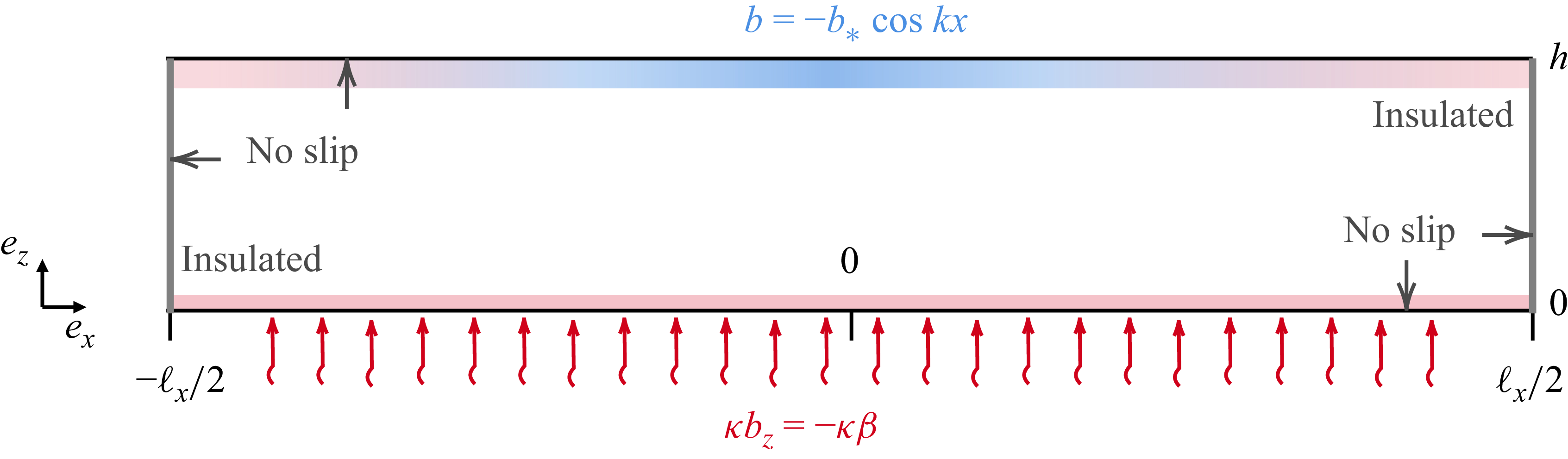
 F=κβ
F=κβ
 0.02h2/κ
 (a)
(a) RaH=3.35×10⁶
 (b)
(b) RaH=2.03×10⁷
 RaV=107
 Γ=8
Γ=8 Pr=1
Pr=1 νκ/h3
νκ/h3
 RaV
RaV b⋆
b⋆ (a)
(a) βh
βh (b)
(b) δ
δ b¯z(z)
 95%
95% b¯z
b¯z Γ=8
Γ=8 Pr=1
Pr=1
 (a)
(a) RaHN
RaHN RaH
RaH ⟨bz⟩=0
 RaV
RaV RaV
RaV RaV
RaV 109
109 1010
1010 Γ=8
Γ=8 (b)
(b) RaHS
RaHS RaH
RaH ⟨bz⟩=β
 RaV
RaV RaV
RaV RaV
RaV 109
109 Γ=8
Γ=8
 b¯z
b¯z RaV
RaV RaH=102
 (a)
(a) (a)
(a) RaV=108
 RaV=108
 RaH=102
 (b)
(b) δ
δ RaV
RaV (c)
(c) |⟨bz⟩|
 RaV
RaV
 b¯z
b¯z RaH
RaH RaV=102
 (a)
(a) RaH=108
 RaH=108
 RaV=102
 (b)
(b) δ
δ RaH
RaH (c)
(c) ⟨bz⟩
⟨bz⟩ RaH
RaH
 β
β RaH=3.35×10⁶
 Pr=13
Pr=13 Pr=1
Pr=1 Pr=1
Pr=1 RaV=107
 Γ=8
Γ=8
 ⟨⋅⟩vol
 (a)
(a) ⟨ub⟩vol/(κβ)
 (b)
(b) ⟨bz⟩vol/β
 (c)
(c) (e)
(e) ⟨bz⟩/β=−0.121
 (RaH,RaV)=(106,107)
 (Γ,Pr)=(32,1)
 (a)
(a) (b)
(b) ⟨bz/β⟩vol
 (c)
(c) (d)
(d) (a)
(a) ⟨bz⟩/β=1.45×10−2
 (RaH,RaV)=(0.2,1)×108
 (Γ,Pr)=(8,1)
 (a)
(a) εvol/(κβ)
 (a)
(a) χvol/(κβ2)
 εvol=ν⟨|∇u|2⟩vol
 χvol=κ⟨|∇b|2⟩vol
 ℓy/h=1/8
 ℓy/h=1
 (RaH,RaV)=(0.2,1)×108
 (Γ,Pr)=(8,1)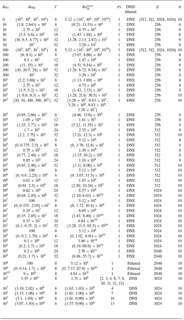

 (a)
(a) X=1/2
X=1/2 RaH∈[10,30,100,300,1000]
 RaV=1000
 (b)
(b) b¯z
b¯z RaV∈[10,30,100,300,1000]
 RaH=1000
 ∘
∘ (a)
(a) (b)
(b) Γ=32
Γ=32 Pr=1.0
 (a)
(a) RaHN
RaHN (b)
(b) RaHS
RaHS RaV
RaV Γ
Γ
 Open access

