


1 Introduction
Coupled flow systems containing a porous-medium layer surrounded by a free-fluid region appear in various environmental settings, biological and technical applications such as interaction of surface water with groundwater, filtration processes and transport of therapeutic agents in blood vessels and tissues. Mass, momentum and energy exchange processes at the fluid–porous interface are complex and they significantly influence fluid flow in the two flow regions. Therefore, the correct choice of interface conditions is crucial for accurate numerical simulations of coupled porous-medium and free-flow problems.
Different models describing free-fluid flow and flow through the porous medium exist in the literature depending on the flow regime and the application of interest. In the most general case the Navier–Stokes equations are used to describe fluid flow in the free-flow domain and multiphase Darcy’s law is applied in the porous medium (Discacciati & Quarteroni Reference Discacciati and Quarteroni2009; Mosthaf et al. Reference Mosthaf, Baber, Flemisch, Helmig, Leijnse, Rybak and Wohlmuth2011). For low Reynolds numbers the Stokes equations can be applied to describe fluid flow in the free-flow domain, and they are coupled to the single-phase Darcy’s law in the porous medium (Discacciati, Miglio & Quarteroni Reference Discacciati, Miglio and Quarteroni2002; Layton, Schieweck & Yotov Reference Layton, Schieweck and Yotov2003; Angot, Goyeau & Ochoa-Tapia Reference Angot, Goyeau and Ochoa-Tapia2017). This problem formulation is the most widely used in the last decade both for mathematical modelling (Discacciati et al. Reference Discacciati, Miglio and Quarteroni2002; Jäger & Mikelić Reference Jäger and Mikelić2009; Angot et al. Reference Angot, Goyeau and Ochoa-Tapia2017) and development and analysis of efficient numerical algorithms (Kanschat & Rivière Reference Kanschat and Rivière2010; Layton, Tran & Xiong Reference Layton, Tran and Xiong2012; Rybak et al. Reference Rybak, Magiera, Helmig and Rohde2015; Discacciati & Gerardo-Giorda Reference Discacciati and Gerardo-Giorda2018) for coupled flow systems. Other models can be used in the two flow domains, e.g. the shallow water equations for the free-surface flow coupled to the Richards equation in the unsaturated zone (Dawson Reference Dawson2008; Sochala, Ern & Piperno Reference Sochala, Ern and Piperno2009) or hydrostatic equations with the free surface coupled to Darcy’s law in the subsurface (Reuter et al. Reference Reuter, Rupp, Aizinger and Knabner2019).
In this paper, we consider the classical coupled problem consisting of the Stokes equations in the free-flow domain, the single-phase Darcy’s law in the porous medium and the conservation of mass, the balance of normal forces and the Beavers–Joseph coupling condition (Beavers & Joseph Reference Beavers and Joseph1967) at the fluid–porous interface. We demonstrate that the Beavers–Joseph condition and its variations (Saffman Reference Saffman1971; Jones Reference Jones1973; Nield Reference Nield2009) are not suitable for arbitrary flow directions. Nevertheless, they are widely used not only for the parallel flow to the interface (regime for which the conditions were initially postulated (Beavers & Joseph Reference Beavers and Joseph1967) and then rigorously derived (Jäger & Mikelić Reference Jäger and Mikelić2009)) but also for industrial filtration (Hanspal et al. Reference Hanspal, Waghode, Nassehi and Wakeman2009; Kanschat & Rivière Reference Kanschat and Rivière2010; Discacciati & Gerardo-Giorda Reference Discacciati and Gerardo-Giorda2018). For infiltration problems where the fluid flow is perpendicular to the fluid–porous interface alternative coupling conditions are proposed in Carraro et al. (Reference Carraro, Goll, Marciniak-Czochra and Mikelić2015). However, these conditions are developed for a very specific boundary value problem and therefore are not applicable to general coupled flow problems. Recently proposed interface conditions in Angot et al. (Reference Angot, Goyeau and Ochoa-Tapia2017) contain several parameters which are unknown and need to be fitted. Coupling conditions with effective coefficients that can be computed numerically based on the pore geometry are developed in Lācis et al. (Reference Lācis, Sudhakar, Pasche and Bagheri2019) but validated only for the flow parallel to the interface. There are several other attempts to validate the classical set of interface conditions (Le Bars & Worster Reference Le Bars and Worster2006; Zampogna & Bottaro Reference Zampogna and Bottaro2016; Lācis & Bagheri Reference Lācis and Bagheri2017), however, not for arbitrary flows. Numerical study of a turbulent flow over porous media is performed recently in Yang et al. (Reference Yang, Coltman, Weishaupt, Terzis, Helmig and Weigand2019).
The goal of this work is to demonstrate that the widely used Beavers–Joseph and Beavers–Joseph–Saffman interface conditions fail for arbitrary flow directions and to provide a benchmark which can be used by researchers working on the development of alternative interface conditions for coupled free-flow and porous-medium systems (Carraro et al. Reference Carraro, Goll, Marciniak-Czochra and Mikelić2015; Lācis & Bagheri Reference Lācis and Bagheri2017; Lācis et al. Reference Lācis, Sudhakar, Pasche and Bagheri2019). To the best of our knowledge, such a validation study of the Beavers–Joseph interface condition for the Stokes–Darcy coupling does not exist in the literature.
The paper is organised as follows. We provide the flow system description at the microscale and the coupled macroscale Stokes–Darcy model in § 2. The macroscale model requires the effective permeability which we compute using the homogenisation approach presented in § 3 for different geometrical configurations. Numerical simulation results for two different infiltration scenarios and different configurations of porous media are presented in § 4. Finally, the summary is provided in § 5.
2 Coupled problem formulation
2.1 Geometrical setting and assumptions
Fluid flow in coupled free-flow and porous-medium systems can be described from the microscale and the macroscale perspective. At the microscale, the pore geometry is resolved and the (Navier–)Stokes equations are solved in the flow domain  $\unicode[STIX]{x1D6FA}^{\unicode[STIX]{x1D700}}$ which consists of the free-flow region $\unicode[STIX]{x1D6FA}_{f\,f}$ and the pore space of the porous medium $\unicode[STIX]{x1D6FA}_{pm}^{\unicode[STIX]{x1D700}}$. At the macroscale, two flow regions (free flow $\unicode[STIX]{x1D6FA}_{f\,f}$ and porous medium $\unicode[STIX]{x1D6FA}_{pm}$) are treated as two different continua and two different models are applied in these domains. These macroscale models need to be coupled at the fluid–porous interface $\unicode[STIX]{x1D6E4}$ (figure 1). In this paper, we consider $\unicode[STIX]{x1D6E4}$ to be sharp, $\unicode[STIX]{x1D6E4}=\unicode[STIX]{x2202}\unicode[STIX]{x1D6FA}_{f\,f}\cap \unicode[STIX]{x2202}\unicode[STIX]{x1D6FA}_{pm}$, and simple, i.e. it cannot store mass and momentum, and thermodynamic properties cannot be transported along $\unicode[STIX]{x1D6E4}$.
Geometrical setting of filtration problem 1.
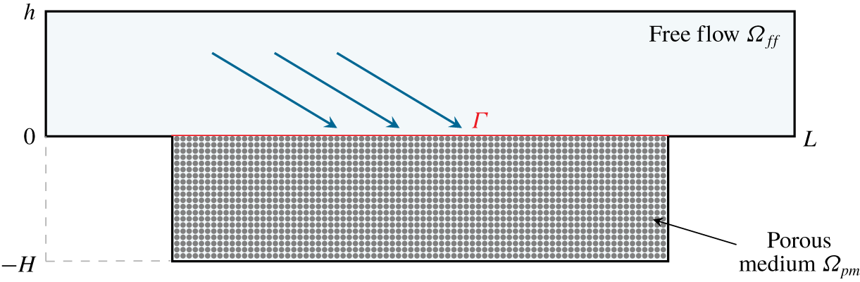
The free-flow domain is filled by a single fluid phase containing a single chemical species, and the same fluid fully saturates the porous medium. The fluid is assumed to be incompressible having also constant viscosity. The temperature is constant, therefore the energy balance equation does not appear in the model formulation. The flow is considered to be at low Reynolds numbers, so that the Stokes equations can be used to describe the flow regime.
To be able to determine effective properties of the coupled model in a relative simple way, we consider porous media with periodically distributed solid inclusions (figures 2 and 6). The microscale and macroscale are assumed to be separable, i.e.  $\unicode[STIX]{x1D700}=\ell /L\ll 1$ where $\ell$ is the characteristic pore size and $L$ is the length of the domain (figure 2). The theory of homogenisation (Hornung Reference Hornung1997; Auriault, Boutin & Geindreau Reference Auriault, Boutin and Geindreau2009; Schulz et al. Reference Schulz, Ray, Zech, Rupp and Knabner2019) is applied to compute the effective permeability. Different geometrical configurations are considered (figures 2 and 6) leading to diverse anisotropic porous media (see permeability in (4.3), (4.6), (4.8), (4.9)) and different filtration problems are modelled (figures 1, 3 and 9). The details are given in § 4.
2.2 Microscale model
Fluid flow in the domain  $\unicode[STIX]{x1D6FA}^{\unicode[STIX]{x1D700}}=\unicode[STIX]{x1D6FA}_{f\,f}\cup \unicode[STIX]{x1D6FA}_{pm}^{\unicode[STIX]{x1D700}}$ is described by the non-dimensional steady Stokes equations completed with the no-slip condition on the fluid–solid interface
 $$\begin{eqnarray}\left.\begin{array}{@{}c@{}}\displaystyle \unicode[STIX]{x1D735}\boldsymbol{\cdot }\boldsymbol{v}^{\unicode[STIX]{x1D700}}=0\quad \text{in }\unicode[STIX]{x1D6FA}^{\unicode[STIX]{x1D700}},\\ \displaystyle -\unicode[STIX]{x1D735}\boldsymbol{\cdot }\unicode[STIX]{x1D64F}(\boldsymbol{v}^{\unicode[STIX]{x1D700}},p^{\unicode[STIX]{x1D700}})-\unicode[STIX]{x1D70C}\boldsymbol{g}=\mathbf{0}\quad \text{in }\unicode[STIX]{x1D6FA}^{\unicode[STIX]{x1D700}},\\ \displaystyle \boldsymbol{v}^{\unicode[STIX]{x1D700}}=\mathbf{0}\quad \text{on }\unicode[STIX]{x2202}\unicode[STIX]{x1D6FA}^{\unicode[STIX]{x1D700}}\setminus \unicode[STIX]{x2202}\unicode[STIX]{x1D6FA},\end{array}\right\}\end{eqnarray}$$
 where  $\boldsymbol{v}^{\unicode[STIX]{x1D700}}$ and $p^{\unicode[STIX]{x1D700}}$ are the microscale velocity and pressure, $\unicode[STIX]{x1D70C}$ is the fluid density, $\boldsymbol{g}$ is the gravitational acceleration, $\unicode[STIX]{x1D64F}(\boldsymbol{v}^{\unicode[STIX]{x1D700}},p^{\unicode[STIX]{x1D700}})=2\unicode[STIX]{x1D707}\unicode[STIX]{x1D63F}(\boldsymbol{v}^{\unicode[STIX]{x1D700}})-p^{\unicode[STIX]{x1D700}}\unicode[STIX]{x1D644}$ is the stress tensor, $\unicode[STIX]{x1D707}$ is the dynamic viscosity, $\unicode[STIX]{x1D63F}(\boldsymbol{v}^{\unicode[STIX]{x1D700}})={\textstyle \frac{1}{2}}(\unicode[STIX]{x1D735}\boldsymbol{v}^{\unicode[STIX]{x1D700}}+(\unicode[STIX]{x1D735}\boldsymbol{v}^{\unicode[STIX]{x1D700}})^{\text{T}})$ is the rate of strain tensor and $\unicode[STIX]{x1D644}$ is the identity tensor.
The following boundary conditions are prescribed on the external boundary
 $$\begin{eqnarray}\boldsymbol{v}^{\unicode[STIX]{x1D700}}=\overline{\boldsymbol{v}}\quad \text{on }\unicode[STIX]{x1D6E4}_{D},\quad \unicode[STIX]{x1D64F}(\boldsymbol{v}^{\unicode[STIX]{x1D700}},p^{\unicode[STIX]{x1D700}})\boldsymbol{\cdot }\boldsymbol{n}=\overline{\boldsymbol{t}}\quad \text{on }\unicode[STIX]{x1D6E4}_{N},\end{eqnarray}$$
 where  $\unicode[STIX]{x1D6FA}=\unicode[STIX]{x1D6FA}_{pm}\cup \unicode[STIX]{x1D6FA}_{f\,f}$, $\boldsymbol{n}$ is the unit outward normal vector from domain $\unicode[STIX]{x1D6FA}$ on its boundary, $\unicode[STIX]{x2202}\unicode[STIX]{x1D6FA}=\unicode[STIX]{x1D6E4}_{D}\cup \unicode[STIX]{x1D6E4}_{N}$ and $\overline{\boldsymbol{v}}$, $\overline{\boldsymbol{t}}$ are given.
Resolving the pore-scale geometry (see e.g. figure 2) for the microscale problem (2.1)–(2.2) is computationally expensive for realistic applications. Therefore, the macroscale coupled Stokes–Darcy problem with the appropriate set of interface conditions is usually solved. We consider the pore-scale resolved model (2.1)–(2.2) only to validate the interface conditions for the Stokes–Darcy problem presented in § 2.3 for different porous-medium geometries and flow regimes.
2.3 Macroscale coupled model
From the macroscale perspective, the fluid flow in the coupled system is described by the Stokes equations in domain  $\unicode[STIX]{x1D6FA}_{f\,f}$, the Darcy law in domain $\unicode[STIX]{x1D6FA}_{pm}$ and the corresponding set of interface conditions at the fluid–porous interface $\unicode[STIX]{x1D6E4}$.
2.3.1 Free-flow model
Under the assumptions given in § 2.1, the flow in the free-flow domain  $\unicode[STIX]{x1D6FA}_{f\,f}$ is governed by the Stokes equations
 $$\begin{eqnarray}\left.\begin{array}{@{}c@{}}\displaystyle \unicode[STIX]{x1D735}\boldsymbol{\cdot }\boldsymbol{v}=0\quad \text{in }\unicode[STIX]{x1D6FA}_{f\,f},\\ \displaystyle -\unicode[STIX]{x1D735}\boldsymbol{\cdot }\unicode[STIX]{x1D64F}(\boldsymbol{v},p)-\unicode[STIX]{x1D70C}\boldsymbol{g}=\mathbf{0}\quad \text{in }\unicode[STIX]{x1D6FA}_{f\,f},\end{array}\right\}\end{eqnarray}$$
 where  $\boldsymbol{v}$ is the fluid velocity and $p$ is the pressure.
The following boundary conditions are prescribed on the external boundary of the free-flow domain  $\unicode[STIX]{x1D6E4}_{f\,f}=\unicode[STIX]{x2202}\unicode[STIX]{x1D6FA}_{f\,f}\setminus \unicode[STIX]{x1D6E4}$:
 $$\begin{eqnarray}\boldsymbol{v}=\overline{\boldsymbol{v}}_{f\,f}\quad \text{on }\unicode[STIX]{x1D6E4}_{D,f\,f},\quad \unicode[STIX]{x1D64F}(\boldsymbol{v},p)\boldsymbol{\cdot }\boldsymbol{n}_{f\,f}=\overline{\boldsymbol{t}}_{f\,f}\quad \text{on }\unicode[STIX]{x1D6E4}_{N,f\,f},\end{eqnarray}$$
 where  $\boldsymbol{n}_{f\,f}$ is the unit outward normal vector from the domain $\unicode[STIX]{x1D6FA}_{f\,f}$ on its boundary, $\unicode[STIX]{x1D6E4}_{f\,f}=\unicode[STIX]{x1D6E4}_{D,f\,f}\cup \unicode[STIX]{x1D6E4}_{N,f\,f}$ and $\overline{\boldsymbol{v}}_{f\,f}$, $\overline{\boldsymbol{t}}_{f\,f}$ are given.
2.3.2 Porous-medium model
The Darcy flow equations describe fluid flow through the porous medium
 $$\begin{eqnarray}\unicode[STIX]{x1D735}\boldsymbol{\cdot }\boldsymbol{v}=q,\quad \boldsymbol{v}=-\frac{\unicode[STIX]{x1D646}}{\unicode[STIX]{x1D707}}(\unicode[STIX]{x1D735}p-\unicode[STIX]{x1D70C}\boldsymbol{g})\quad \text{in }\unicode[STIX]{x1D6FA}_{pm},\end{eqnarray}$$
 where  $\boldsymbol{v}$ is the velocity of the fluid through the porous medium, $q$ is the source term and $\unicode[STIX]{x1D646}$ is the intrinsic permeability tensor which is symmetric, positive definite and bounded.
We define the following boundary conditions on the external boundary of the porous-medium domain  $\unicode[STIX]{x1D6E4}_{pm}=\unicode[STIX]{x2202}\unicode[STIX]{x1D6FA}_{pm}\setminus \unicode[STIX]{x1D6E4}$:
 $$\begin{eqnarray}p=\overline{p}_{pm}\quad \text{on }\unicode[STIX]{x1D6E4}_{D,pm},\quad \boldsymbol{v}\boldsymbol{\cdot }\boldsymbol{n}_{pm}=\overline{v}_{pm}\quad \text{on }\unicode[STIX]{x1D6E4}_{N,pm},\end{eqnarray}$$
 where  $\boldsymbol{n}_{pm}$ is the unit outward normal vector from the domain $\unicode[STIX]{x1D6FA}_{pm}$ on its boundary, $\unicode[STIX]{x1D6E4}_{pm}=\unicode[STIX]{x1D6E4}_{D,pm}\cup \unicode[STIX]{x1D6E4}_{N,pm}$, $\unicode[STIX]{x1D6E4}_{D,pm}\cap \unicode[STIX]{x1D6E4}_{N,pm}=\emptyset$, $\unicode[STIX]{x1D6E4}_{D,pm}\neq \emptyset$ and $\overline{p}_{pm}$, $\overline{v}_{pm}$ are given.
In order to complete the model formulation (2.3)–(2.6), an appropriate set of interface conditions has to be defined on the fluid–porous interface  $\unicode[STIX]{x1D6E4}$. The choice of these conditions is crucial for physically consistent and accurate description of the coupled problem.
2.3.3 Interface conditions
Two different flow regimes are considered in the literature: flow almost parallel and flow almost perpendicular to the porous medium. Different sets of interface conditions have been proposed for these two cases. However, both for numerical analysis and simulation, the following interface conditions are typically applied: the conservation of mass, the balance of normal forces and the Beavers–Joseph condition for the tangential component of velocity. We concentrate on this widely used setting in the paper and show that the Beavers–Joseph condition and also its modifications are not suitable for arbitrary flow directions. We use the subscripts ( $f\,f$, $pm$) to define the velocity and pressure at the interface coming from two different flow domains.
The mass conservation across the fluid–porous interface is
 $$\begin{eqnarray}\boldsymbol{v}_{f\,f}\boldsymbol{\cdot }\boldsymbol{n}=\boldsymbol{v}_{pm}\boldsymbol{\cdot }\boldsymbol{n}\quad \text{on }\unicode[STIX]{x1D6E4},\end{eqnarray}$$
and the balance of normal forces is given by
 $$\begin{eqnarray}-\boldsymbol{n}\boldsymbol{\cdot }\unicode[STIX]{x1D64F}(\boldsymbol{v}_{f\,f},p_{f\,f})\boldsymbol{\cdot }\boldsymbol{n}=p_{pm}\quad \text{on }\unicode[STIX]{x1D6E4},\end{eqnarray}$$
 where  $\boldsymbol{n}$ is the unit normal vector at the interface $\unicode[STIX]{x1D6E4}$ pointing outward from the free-flow domain $\unicode[STIX]{x1D6FA}_{f\,f}$.
Several possibilities exist in the literature for the coupling condition on the tangential velocity component. The most widely used one is the Beavers–Joseph interface condition (Beavers & Joseph Reference Beavers and Joseph1967; Jones Reference Jones1973)
 $$\begin{eqnarray}(\boldsymbol{v}_{f\,f}-\boldsymbol{v}_{pm})\boldsymbol{\cdot }\unicode[STIX]{x1D749}_{j}+\frac{2\sqrt{\unicode[STIX]{x1D646}}}{\unicode[STIX]{x1D6FC}_{BJ}}\boldsymbol{n}\boldsymbol{\cdot }\unicode[STIX]{x1D63F}(\boldsymbol{v}_{f\,f})\boldsymbol{\cdot }\unicode[STIX]{x1D749}_{j}=0,\quad j=1,\ldots ,d-1,\text{ on }\unicode[STIX]{x1D6E4},\end{eqnarray}$$
 where  $\unicode[STIX]{x1D6FC}_{BJ}>0$ is the Beavers–Joseph parameter, $\unicode[STIX]{x1D646}$ is the effective permeability tensor, $\unicode[STIX]{x1D749}_{j}$ is a unit vector tangential to the interface and $d$ is the number of space dimensions. Saffman (Reference Saffman1971) proposed a modification of condition (2.9) such that the tangential free-flow velocity is proportional to the shear stress
 $$\begin{eqnarray}\boldsymbol{v}_{f\,f}\boldsymbol{\cdot }\unicode[STIX]{x1D749}_{j}+\frac{2\sqrt{\unicode[STIX]{x1D646}}}{\unicode[STIX]{x1D6FC}_{BJ}}\boldsymbol{n}\boldsymbol{\cdot }\unicode[STIX]{x1D63F}(\boldsymbol{v}_{f\,f})\boldsymbol{\cdot }\unicode[STIX]{x1D749}_{j}=0,\quad j=1,\ldots ,d-1,\text{on }\unicode[STIX]{x1D6E4}.\end{eqnarray}$$
The interface condition (2.10) is no more a coupling condition but a boundary condition for the tangential component of the free-flow velocity. However, this simplification does not remain true for general coupled flow problems, it is only valid if the filtration velocity is much smaller than the slip velocity and thus can be neglected. We consider both conditions (2.9) and (2.10) for numerical simulations in § 4.
Different approaches to compute  $\sqrt{\unicode[STIX]{x1D646}}$ are used in the literature (see table 1). These definitions are all identical when the porous medium is isotropic, i.e. $\unicode[STIX]{x1D646}=k\unicode[STIX]{x1D644}$, $k\in \mathbb{R}^{+}$. However, this is not always the case and porous media are often anisotropic. There are two possibilities for anisotropy: $\unicode[STIX]{x1D646}=\operatorname{diag}\{k_{11},\ldots ,k_{dd}\}$ or $\unicode[STIX]{x1D646}=(k_{ij})_{1\leqslant i,j\leqslant d}$ is a full tensor, i.e. $k_{ij}\neq 0$.


3 Effective permeability computation
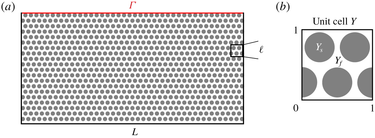
To obtain the effective permeability for coupled macroscale models we use the theory of homogenisation (Hornung Reference Hornung1997). Therefore, we consider porous media with periodic microstructure such that the different length scales can be separated  $\unicode[STIX]{x1D700}=\ell /L\ll 1$ (figure 2a). The structure of the porous medium is obtained by periodic repetition of the unit cell $Y=(0,1)^{2}$ scaled with $\unicode[STIX]{x1D700}$ (figure 2b). Following the idea of homogenisation with two-scale asymptotic expansions (Hornung Reference Hornung1997; Auriault et al. Reference Auriault, Boutin and Geindreau2009), we study the behaviour of the solutions $(\boldsymbol{v}^{\unicode[STIX]{x1D700}},p^{\unicode[STIX]{x1D700}})$ to the microscopic problem (2.1) for $\unicode[STIX]{x1D700}\rightarrow 0$ and obtain Darcy’s law (2.5) as the upscaled flow model in the porous-medium domain $\unicode[STIX]{x1D6FA}_{pm}$.
The permeability tensor  $\widetilde{\unicode[STIX]{x1D646}}$ is given by
 $$\begin{eqnarray}\widetilde{\unicode[STIX]{x1D646}}=(\widetilde{k}_{ij})_{1\leqslant i,j\leqslant d}=\int _{Y_{f}}w_{i}^{\,j}\,\text{d}\boldsymbol{y},\end{eqnarray}$$
 where  $\boldsymbol{w}^{j}=(w_{1}^{\,j},\ldots ,w_{d}^{\,j})$ and $\unicode[STIX]{x03C0}^{j}$ are the solutions to the following cell problems for $j=1,\ldots ,d$:
 $$\begin{eqnarray}\left.\begin{array}{@{}c@{}}\displaystyle -\unicode[STIX]{x1D6E5}_{\boldsymbol{y}}\boldsymbol{w}^{j}+\unicode[STIX]{x1D735}_{\boldsymbol{y}}\unicode[STIX]{x03C0}^{j}=\boldsymbol{e}_{j}\quad \text{in }Y_{f},\\ \displaystyle \unicode[STIX]{x1D735}_{\boldsymbol{y}}\boldsymbol{\cdot }\boldsymbol{w}^{j}=0\quad \text{in }Y_{f},\\ \displaystyle \boldsymbol{w}^{j}=\mathbf{0}\quad \text{on }\unicode[STIX]{x2202}Y_{f}\setminus \unicode[STIX]{x2202}Y,\\ \displaystyle \{\boldsymbol{w}^{j},\unicode[STIX]{x03C0}^{j}\}\text{ is 1-periodic}\text{ in }\boldsymbol{y},\quad \int _{Y_{f}}\unicode[STIX]{x03C0}^{j}\,\text{d}\boldsymbol{y}=0,\quad \boldsymbol{y}=\frac{\boldsymbol{x}}{\unicode[STIX]{x1D700}}.\end{array}\right\}\end{eqnarray}$$
 The unit cell  $Y$ for two-dimensional problems ( $d=2$) is presented in figure 2(b). The effective permeability $\unicode[STIX]{x1D646}$ is obtained by scaling tensor $\widetilde{\unicode[STIX]{x1D646}}$ with $\unicode[STIX]{x1D700}^{2}$.
(a) Schematic geometrical configuration of the periodic porous medium with circular inclusions. (b) Unit cell for computing effective parameters.
4 Model validation
In this section, we show that the Beavers–Joseph interface condition (2.9) and the Beavers–Joseph–Saffman interface condition (2.10) are not suitable for many coupled Stokes–Darcy (SD) problems. For this purpose we compare numerical simulation results for the pore-scale resolved models and the corresponding macroscale Stokes–Darcy models.
The Stokes–Darcy coupling is well studied in the literature (Layton et al. Reference Layton, Schieweck and Yotov2003; Jäger & Mikelić Reference Jäger and Mikelić2000, Reference Jäger and Mikelić2009; Discacciati & Quarteroni Reference Discacciati and Quarteroni2009; Kanschat & Rivière Reference Kanschat and Rivière2010). However, the geometrical configuration of the porous medium is often assumed to be very simple, e.g. made up of circular inclusions which are structured in rows and columns in line, and the fluid flow parallel to the fluid–porous interface. In this case, the Beavers–Joseph condition (2.9) is suitable to couple the macroscale models. Rybak et al. (Reference Rybak, Schwarzmeier, Eggenweiler and Rüde2019) showed that this condition is also applicable when the flow is almost perpendicular to the interface. In this paper, we consider flow regimes with arbitrary flow directions (figures 1, 3 and 9) and we study different geometrical configurations for the porous-medium domain (figures 2 and 6).
For the microscale numerical simulations we use the software package FreeFEM++ with P2-P1 finite elements (Hecht Reference Hecht2012). The whole domain  $\unicode[STIX]{x1D6FA}^{\unicode[STIX]{x1D700}}$ is resolved by approx. 360 000 elements and between two solid inclusions there are at least 3 elements. The cell problems (3.2) are also solved with FreeFEM++ using the P2-P1 Taylor–Hood finite element pair and considering the triangulation of $Y_{f}$ with approx. 50 000 elements. The dynamic viscosity of the fluid is scaled to $\unicode[STIX]{x1D707}=1$ for all test cases and gravitational effects are neglected ( $\boldsymbol{g}=\mathbf{0}$). We discretise the macroscale problem using the finite volume method on staggered grids (Versteeg & Malalasekra Reference Versteeg and Malalasekra2007) computing the pressure in the cell centres and the velocities at the cell edges. The computational domains $\unicode[STIX]{x1D6FA}_{f\,f}$ and $\unicode[STIX]{x1D6FA}_{pm}$ are partitioned into equal blocks of size $1/400\times 1/400$ with conforming grids at the interface $\unicode[STIX]{x1D6E4}$.
In the following, we present two different filtration problems. The first problem (figure 1) is studied in detail in § 4.1, considering different flow regimes (parallel and arbitrary to the interface) and various types of porous media. One configuration of the porous medium is made up of staggered rows containing circular inclusions (figure 2) and the other ones consist of oval inclusions tilted to the right or tilted to the left (figure 6). The second example of a filtration problem is presented in § 4.2 to show that the studied filtration problem 1 is not the only coupled Stokes–Darcy system where the Beavers–Joseph interface condition is unsuitable. For this second validation problem we waive a detailed study due to similar results as in § 4.1.
4.1 Filtration problem 1
We consider the geometrical setting presented in figure 1 with the free-flow domain  $\unicode[STIX]{x1D6FA}_{f\,f}=[0,3]\times [0,0.5]$, the porous region $\unicode[STIX]{x1D6FA}_{pm}=[0.5,2.5]\times [-0.5,0]$ and the interface $\unicode[STIX]{x1D6E4}=[0.5,2.5]\times \{0\}$ for the first filtration problem.
For the pore-scale resolved model (2.1)–(2.2) we specify the following boundary conditions on the external boundary
 $$\begin{eqnarray}\left.\begin{array}{@{}c@{}}\displaystyle \overline{\boldsymbol{v}}=\mathbf{0}\quad \text{on }\unicode[STIX]{x2202}\unicode[STIX]{x1D6FA}\setminus (\{x_{1}=0\}\cup \{x_{2}=-0.5\}),\\ \displaystyle \overline{\boldsymbol{v}}=(0.1\sin (2\unicode[STIX]{x03C0}x_{2}),0)\quad \text{on }\{x_{1}=0\},\\ \displaystyle \overline{\boldsymbol{t}}=(0,-10)\quad \text{on }\{x_{2}=-0.5\}.\end{array}\right\}\end{eqnarray}$$
The Stokes–Darcy problem (2.3)–(2.9) is solved with the corresponding boundary conditions
 $$\begin{eqnarray}\left.\begin{array}{@{}c@{}}\displaystyle \overline{\boldsymbol{v}}_{f\,f}=\mathbf{0}\quad \text{on }\{x_{1}=3\}\cup \{x_{2}=0.5\},\\ \displaystyle \overline{\boldsymbol{v}}_{f\,f}=(0.1\sin (2\unicode[STIX]{x03C0}x_{2}),0)\quad \text{on }\{x_{1}=0\},\\ \displaystyle \overline{v}_{pm}=0\quad \text{on }\{x_{1}=0.5\}\cup \{x_{1}=2.5\},\\ \displaystyle \overline{p}_{pm}=10\quad \text{on }\{x_{2}=-0.5\}.\end{array}\right\}\end{eqnarray}$$
 We recall that the Beavers–Joseph condition (2.9) is the most commonly used coupling condition for the tangential component of velocity. Therefore, unless stated otherwise, we use it for the validation cases. To compute  $\sqrt{\unicode[STIX]{x1D646}}$ needed in condition (2.9), we use the second interpretation from table 1. Since the interface is parallel to the $x_{1}$-axis in all validation cases we obtain $\sqrt{\unicode[STIX]{x1D646}}=\sqrt{k_{11}}$. Note that choosing another interpretation of $\sqrt{\unicode[STIX]{x1D646}}$ (see table 1) in this case only results in an appropriate adjustment of the Beavers–Joseph parameter $\unicode[STIX]{x1D6FC}_{BJ}$.
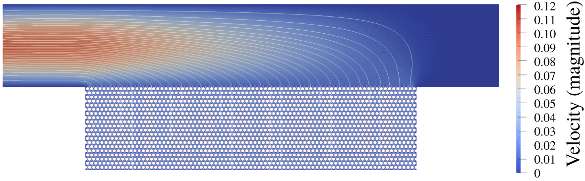
Microscopic flow field for filtration problem 1.
4.1.1 Staggered circular inclusions
In this section, we consider a porous medium consisting of a staggered arrangement of circular solid inclusions (figure 2). There are 80 inclusions in the  $x_{1}$-direction, 20 inclusions in the $x_{2}$-direction and the radius of the inclusions is $r=0.01$. The permeability tensor $\widetilde{\unicode[STIX]{x1D646}}$ is calculated numerically according to (3.1) and for the considered geometry we get
 $$\begin{eqnarray}\widetilde{\unicode[STIX]{x1D646}}=\left(\begin{array}{@{}cc@{}}8.550\times 10^{-4} & 0\\ 0 & 4.141\times 10^{-4}\end{array}\right).\end{eqnarray}$$
 The effective permeability of the porous medium is obtained by scaling  $\unicode[STIX]{x1D646}=\unicode[STIX]{x1D700}^{2}\widetilde{\unicode[STIX]{x1D646}}$, where the actual scale ratio is $\unicode[STIX]{x1D700}=1/20$.
The microscale problem (2.1)–(2.2) and the coupled Stokes–Darcy problem (2.3)–(2.9) with the boundary conditions (4.1) and (4.2), accordingly, describe a flow system where the fluid flow is arbitrary to the fluid–porous interface (figure 3). To validate the applicability of the Beavers–Joseph interface condition (2.9) we evaluate cross-sections in the middle of the porous-medium domain at  $x_{1}=1.5$ and also at $x_{1}=2.2$. For all simulations the fluid–porous interface $\unicode[STIX]{x1D6E4}$ is located at $x_{2}=0$, directly on the top of the first row of solid inclusions as proposed in Lācis et al. (Reference Lācis, Sudhakar, Pasche and Bagheri2019) and Rybak et al. (Reference Rybak, Schwarzmeier, Eggenweiler and Rüde2019). The Beavers–Joseph parameter $\unicode[STIX]{x1D6FC}_{BJ}=1$ is commonly chosen in the literature. Therefore, we use the same value in the interface condition (2.9) for this test case. Figure 4 provides profiles of the horizontal velocity component $v_{1}$ for different cross-sections. At $x_{1}=1.5$ the profiles of the pore-scale resolved model (profile: Microscale) and the macroscale Stokes–Darcy simulations (profile: SD) fit quite well (figure 4a). However, at $x_{1}=2.2$ the profiles in the free-flow region differ substantially (figure 4b). We observe that the profiles of the pore-scale resolved simulations and the macroscale numerical simulations for $\unicode[STIX]{x1D6FC}_{BJ}=1$ do not fit also for other cross-sections away from the horizontal centre of the domain.
Velocity profiles ( $x_{1}$-component) for circular inclusions (a) at $x_{1}=1.5$ and (b) at $x_{1}=2.2$ for filtration problem 1 with the fluid flow arbitrary to the interface.
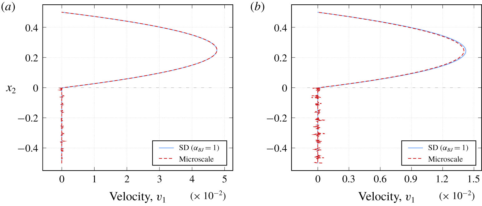
Velocity profiles of the pore-scale resolved model oscillate in the porous-medium domain and near the fluid–porous interface (figure 4) due to the presence of solid inclusions. The Stokes–Darcy model is an upscaled formulation of the microscale problem (2.1) and therefore does not see the microscopic details. For circular solid inclusions we provide the microscale velocity only, not the averaged one, since the physically reasonable oscillations are negligible.
Due to the fact that the filtering velocity in the porous domain is almost zero in this case, there is no preference in taking the Beavers–Joseph condition (2.9) or the Beavers–Joseph–Saffman condition (2.10). There is only a slight difference in the resulting macroscopic profiles. Nevertheless, for this test case, the Beavers–Joseph condition (2.9) and also the Beavers–Joseph–Saffman condition (2.10) are not optimal because one cannot find the value of the parameter  $\unicode[STIX]{x1D6FC}_{BJ}$ such that the velocity profiles of the microscale and macroscale simulation results fit along $\unicode[STIX]{x1D6E4}$.
Remark 1. The Beavers–Joseph interface condition was originally developed to couple the Stokes and Darcy’s models where the fluid flow is almost parallel to the interface. Thus, for such flow systems, it is a suitable coupling condition and the parameter  $\unicode[STIX]{x1D6FC}_{BJ}$ can be fitted so that the macroscale numerical simulations correspond to the pore-scale resolved models.
To validate Remark 1, we consider the same geometry and the same coupled model as before but change the boundary conditions on the external boundary to obtain flow almost parallel to the interface. We apply the following boundary condition on the right boundary of the free-flow domain both for the microscale and the macroscale simulations
 $$\begin{eqnarray}\overline{\boldsymbol{v}}=\overline{\boldsymbol{v}}_{f\,f}=(0.1\sin (2\unicode[STIX]{x03C0}x_{2}),0)\quad \text{on }\{x_{1}=3\}.\end{eqnarray}$$
All the other boundary conditions stay the same as in (4.1) and (4.2).
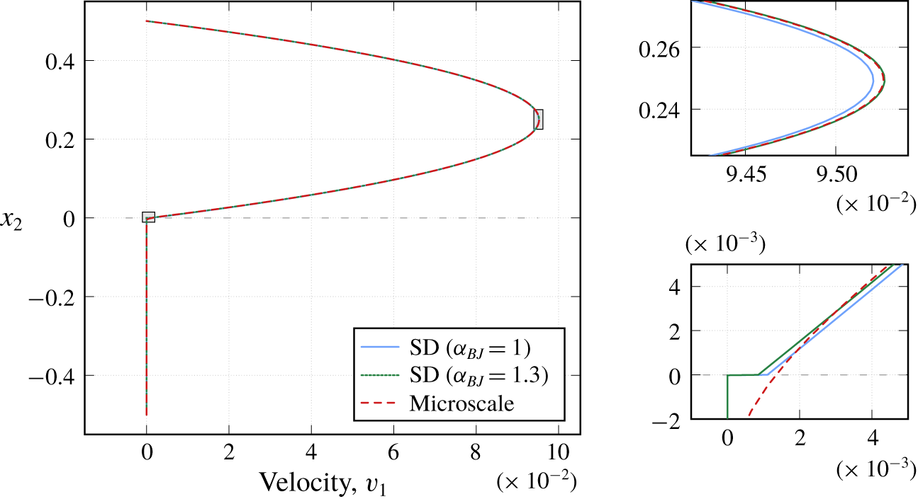
Velocity profiles of the horizontal component at  $x_{1}=2.2$ for this test case are presented in figure 5. We observe that the microscale numerical simulation results are in a good agreement with the macroscale solutions for $\unicode[STIX]{x1D6FC}_{BJ}=1.3$. We should mention that the commonly taken $\unicode[STIX]{x1D6FC}_{BJ}=1$ is not always the optimal choice (figure 5, zoom) even for the Stokes–Darcy problems where the Beavers–Joseph condition is suitable, see also Rybak et al. (Reference Rybak, Schwarzmeier, Eggenweiler and Rüde2019). Due to the reason that the fluid flow is almost parallel to the fluid–porous interface and the filtration into the porous medium is roughly the same along the interface $\unicode[STIX]{x1D6E4}$, velocity profiles at other cross-sections look very similar to those presented in figure 5. Therefore, we do not provide further numerical results for this test case.
Velocity profiles ( $x_{1}$-component) for circular inclusions at $x_{1}=2.2$ for filtration problem 1 with the fluid flow almost parallel to the interface.
4.1.2 Staggered oval inclusions tilted to the right
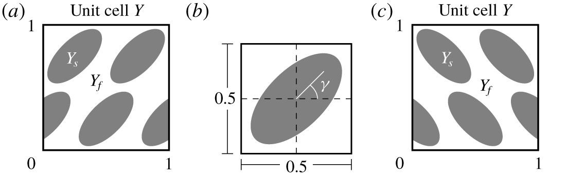
Since the Beavers–Joseph parameter  $\unicode[STIX]{x1D6FC}_{BJ}$ contains information about the interfacial geometry (e.g. surface roughness) we consider further porous-medium configurations (figure 6) in addition to the one presented in figure 2. In this section, the porous medium is generated by unsymmetrical unit cells containing ellipses rotated to the right (figure 6a) that leads to an anisotropic porous medium with a full effective permeability tensor. The porous-medium domain is made up of $80$ oval inclusions in the horizontal direction and $20$ inclusions in the vertical direction distributed periodically in a staggered manner. The semi-major axis of an ellipse is positioned at $\unicode[STIX]{x1D6FE}=\unicode[STIX]{x03C0}/4$ counterclockwise to the positive part of the $x_{1}$-axis (figure 6b). The boundary curves of the solid inclusions within the unit cell $Y$ (figure 6a) are given by the ellipses
 $$\begin{eqnarray}e(t)=(m_{1},m_{2})+0.092(\cos (t)+2\sin (t),-\cos (t)+2\sin (t)),\end{eqnarray}$$
 with the centre  $(m_{1},m_{2})\in \{(0,0.25),(0.5,0.25),(1,0.25),(0.25,0.75),(0.75,0.75)\}$ and $t\in [0,2\unicode[STIX]{x03C0})$ for $m_{1}\in \{0.25,0.5,0.75\}$, $t\in [-0.463648,\unicode[STIX]{x03C0}-0.463648)$ for $m_{1}=0$ and $t\in [\unicode[STIX]{x03C0}-0.463648,2\unicode[STIX]{x03C0}-0.463648)$ for $m_{1}=1$.
(a) Unit cell and (b) construction of one single ellipse in the unit cell for oval inclusions tilted to the right. (c) Unit cell for oval inclusions tilted to the left.
Due to the fact that these inclusions are not symmetric with respect to the  $x_{1}$- and $x_{2}$-axis we obtain the full permeability tensor
 $$\begin{eqnarray}\widetilde{\unicode[STIX]{x1D646}}=\left(\begin{array}{@{}cc@{}}6.4494\times 10^{-4} & 5.1026\times 10^{-4}\\ 5.1026\times 10^{-4} & 1.0512\times 10^{-3}\end{array}\right)\end{eqnarray}$$
 and scale it then  $\unicode[STIX]{x1D646}=\unicode[STIX]{x1D700}^{2}\widetilde{\unicode[STIX]{x1D646}}$ with $\unicode[STIX]{x1D700}=1/20$.
For numerical simulations we use the same equations, interface and boundary conditions (2.3)–(2.9), (4.2) as in § 4.1.1 to obtain fluid flow arbitrary to the fluid–porous interface. In order to make the comparison of microscale to macroscale simulation results in the porous-medium domain easier, we provide additionally the averaged microscale velocity (figures 7 and 8, profile: Avg. microscale). The spatial averaging is done within representative elementary volumes  $V$ in the following manner
 $$\begin{eqnarray}\boldsymbol{v}^{\unicode[STIX]{x1D700},avg}=\frac{1}{|V|}\int _{V_{f}}\boldsymbol{v}^{\unicode[STIX]{x1D700}}\,\text{d}\boldsymbol{x},\end{eqnarray}$$
 where  $V_{f}$ is the fluid part of $V$. The representative elementary volume $V$ coincides with the scaled unit cell $\unicode[STIX]{x1D700}Y$ in the porous-medium domain away from the interface. In the interfacial region, the height of the volume $V$ is scaled with the factors $0.5$ and $0.25$, accordingly. As can be seen from figures 7 and 8 the averaged microscale velocity profiles coincide with the macroscale velocity profiles inside the porous medium away from the interface.
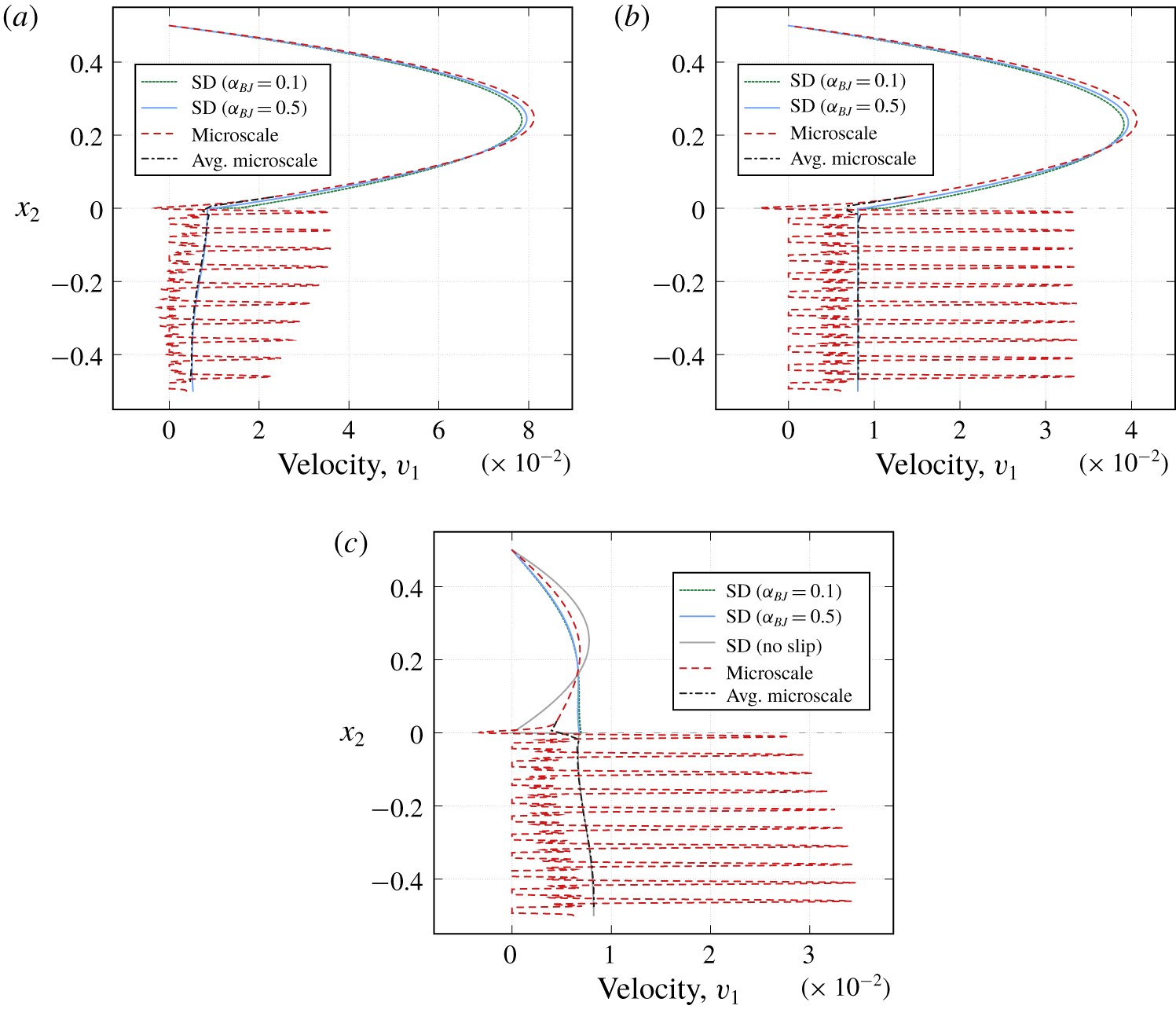
The interface is again located directly on the top of the oval inclusions and we consider the cross-sections at  $x_{1}=0.7$, $x_{1}=1.5$ and $x_{1}=2.2$. Profiles of the horizontal velocity component are provided in figure 7. We observe that in the front part of the porous medium ( $x_{1}=0.7$) the Stokes–Darcy model (2.3)–(2.9), (4.2) with $\unicode[STIX]{x1D6FC}_{BJ}=0.5$ fits the best to the solution of the pore-scale resolved model (2.1)–(2.2), (4.1) (see figure 7a) whereas at $x_{1}=2.2$ the value $\unicode[STIX]{x1D6FC}_{BJ}=0.1$ gives a better fit (figure 7b). Although the choice of $\unicode[STIX]{x1D6FC}_{BJ}=0.1$ provides a better fitting, none of these two values for the Beavers–Joseph parameter is optimal. To obtain a perfect fit of the macroscale to the microscale solution at this cross-section the Beavers–Joseph parameter should be taken $\unicode[STIX]{x1D6FC}_{BJ}<0.1$.
Velocity profiles ( $x_{1}$-component) for oval inclusions tilted to the right (a) at $x_{1}=0.7$, (b) at $x_{1}=2.2$ and (c,d) at $x_{1}=1.5$ for filtration problem 1 with the fluid flow arbitrary to the interface.

Velocity profiles for the cross-sections in the middle of the domain ( $x_{1}=1.5$) are presented in figures 7(c) and 7(d). The macroscale velocity profiles with $\unicode[STIX]{x1D6FC}_{BJ}=0.1$ and $\unicode[STIX]{x1D6FC}_{BJ}=0.5$ both do not correspond with the microscale solution. Here, the optimal value of the parameter $\unicode[STIX]{x1D6FC}_{BJ}$ should be in between of both tested values and can be found experimentally.
We observe that the optimal value of the parameter  $\unicode[STIX]{x1D6FC}_{BJ}$ can be identified only locally, at least for this test case. The Beavers–Joseph parameter $\unicode[STIX]{x1D6FC}_{BJ}$ contains information about the interfacial region (e.g. surface roughness) and since the considered porous medium is homogeneous and periodic and the interface is flat, the properties of the interface do not change and the parameter $\unicode[STIX]{x1D6FC}_{BJ}$ is supposed to be constant. Since we found different parameters $\unicode[STIX]{x1D6FC}_{BJ}$ to be optimal for different cross-sections, we conclude that there exist no global $\unicode[STIX]{x1D6FC}_{BJ}$ along the whole interface.
In addition to the macroscale model with the Beavers–Joseph coupling condition (2.9) we solved the Stokes–Darcy model with the Beavers–Joseph–Saffman interface condition (2.10) and also made cross-sections at  $x_{1}=1.5$ (profile: SD-BJS, see figures 7c and 7d). We observe that the macroscale solutions obtained by using Saffman’s modification do not fit to the microscale simulation results at all. This is due to the fact that for such flow problems the Darcy velocity is relatively high and therefore cannot be neglected as proposed by Saffman.
Comparing different cross-sections for this geometrical configuration one cannot identify any value of  $\unicode[STIX]{x1D6FC}_{BJ}$ as the best choice for the Beavers–Joseph parameter. Summing up, for such coupled flow problems, the commonly used Beavers–Joseph interface condition (2.9) and also the Beavers–Joseph–Saffman condition (2.10) are not suitable to couple the Stokes equations to Darcy’s law.
4.1.3 Staggered oval inclusions tilted to the left
In this section, we consider a porous medium with  $80$ oval inclusions in the $x_{1}$-direction and $20$ inclusions in the $x_{2}$-direction distributed in the same staggered manner as in § 4.1.2. The semi-major axis of an ellipse is rotated $\unicode[STIX]{x03C0}/4$ clockwise to the negative part of the $x_{1}$-axis (figure 6c). In this case, the ellipses within the unit cell $Y$ are given by
 $$\begin{eqnarray}e(t)=(m_{1},m_{2})+0.092(2\cos (t)+\sin (t),-2\cos (t)+\sin (t)),\end{eqnarray}$$
 with the centre  $(m_{1},m_{2})\in \{(0,0.25),(0.5,0.25),(1,0.25),(0.25,0.75),(0.75,0.75)\}$ and $t\in [0,2\unicode[STIX]{x03C0})$ for $m_{1}\in \{0.25,0.5,0.75\}$, $t\in [-1.107149,\unicode[STIX]{x03C0}-1.107149)$ for $m_{1}=0$ and $t\in [\unicode[STIX]{x03C0}-1.107149,2\unicode[STIX]{x03C0}-1.107149)$ for $m_{1}=1$.
Again, as in § 4.1.2, we obtain a full permeability tensor  $\unicode[STIX]{x1D646}=\unicode[STIX]{x1D700}^{2}\widetilde{\unicode[STIX]{x1D646}}$ with $\unicode[STIX]{x1D700}=1/20$ and
 $$\begin{eqnarray}\widetilde{\unicode[STIX]{x1D646}}=\left(\begin{array}{@{}cc@{}}6.4494\times 10^{-4} & -5.1026\times 10^{-4}\\ -5.1026\times 10^{-4} & 1.0512\times 10^{-3}\end{array}\right).\end{eqnarray}$$
Velocity profiles ( $x_{1}$-component) for oval inclusions tilted to the left (a) at $x_{1}=0.7$, (b) at $x_{1}=1.5$ and (c) at $x_{1}=2.2$ for filtration problem 1 with the fluid flow arbitrary to the interface.
We consider cross-sections at  $x_{1}=0.7$, $x_{1}=1.5$ and $x_{1}=2.2$ to evaluate the microscale and the macroscale numerical simulation results. The fluid–porous interface $\unicode[STIX]{x1D6E4}$ is located as before directly on the top of the first row of oval solid inclusions at $x_{2}=0$. Figure 8(a) provides velocity profiles in the left part of the porous medium at $x_{1}=0.7$. We tested different values of the Beavers–Joseph parameter $\unicode[STIX]{x1D6FC}_{BJ}$, however, for all choices the macroscale velocity profiles significantly differ from the pore-scale solution. Velocity profiles for the $x_{1}$-component in the horizontal centre are presented in figure 8(b). Here, one also cannot achieve any fitting between the microscale and macroscale simulation results, no matter which value of $\unicode[STIX]{x1D6FC}_{BJ}$ is chosen. We also provide velocity profiles at $x_{1}=2.2$ (figure 8c) including additionally the no-slip condition for the tangential velocity component (profile: SD (no slip)). In this case, the velocity profile of the pore-scale resolved simulations completely disagree with the profiles of the macroscopic solutions for different values of $\unicode[STIX]{x1D6FC}_{BJ}$ and also with the one belonging to the no-slip condition. We claim that the main factor for these differences is the unsuitable coupling at the interface. For this geometry we observe the same problem for all cross-sections. The parameter $\unicode[STIX]{x1D6FC}_{BJ}$ cannot be adjusted such that the microscale and macroscale profiles fit.
Remark 2. Considering the profiles in figure 8, one could speculate that for the solid inclusions (4.7) the fluid–porous interface  $\unicode[STIX]{x1D6E4}$ is located at a wrong position. To the best of our knowledge, there is no recommendation concerning the interface location for oval inclusions. Therefore, we cannot claim that the location on top of solid grains is valid for all porous structures and all flow regimes. However, we justify our choice as follows: (i) interface location should be the same over the whole length of the porous-medium domain since the medium is periodic; (ii) interface location should be chosen independently on the explicit geometrical configuration of the porous medium while the interface roughness is the same. Since for oval inclusions tipped to the right (4.5) and tipped to the left (4.7) the interface roughness is the same and for some cross-sections the interface location seems to be correct (figure 7), we place the interface directly on the top of the first row of solid inclusions.
4.2 Filtration problem 2
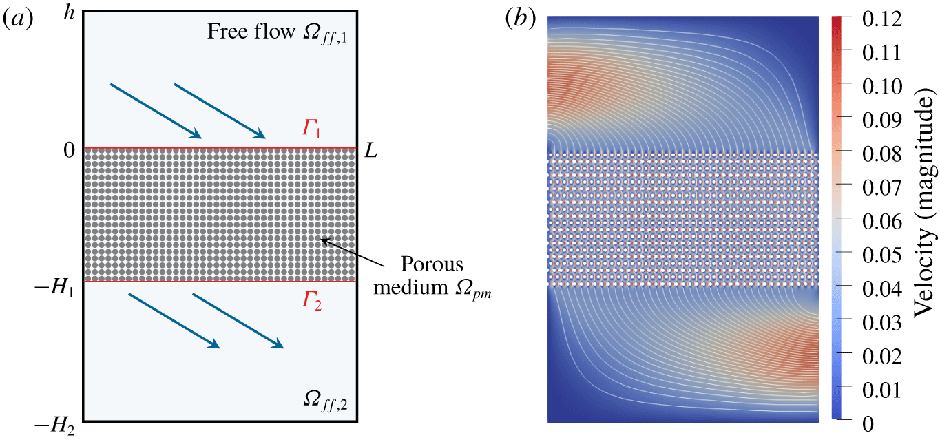
The purpose of this section is to demonstrate that the Beavers–Joseph interface condition (2.9) is unsuitable for many other coupled Stokes–Darcy problems, not only for the setting presented in § 4.1. For the second filtration problem, we consider the geometrical setting schematically presented in figure 9(a). Here, we consider two free-flow regions  $\unicode[STIX]{x1D6FA}_{f\,f,1}=[0,1]\times [0,0.5]$ and $\unicode[STIX]{x1D6FA}_{f\,f,2}=[0,1]\times [-1,-0.5]$ and the porous medium in between $\unicode[STIX]{x1D6FA}_{pm}=[0,1]\times [-0.5,0]$. The free-flow and porous-medium domains are separated by two sharp fluid–porous interfaces $\unicode[STIX]{x1D6E4}_{1}=[0,1]\times \{0\}$ and $\unicode[STIX]{x1D6E4}_{2}=[0,1]\times \{-0.5\}$. The porous medium is made up of the staggered circular inclusions (figure 2) with the radius $r=0.0075$. The scale separation ratio is $\unicode[STIX]{x1D700}=1/20$ and the effective permeability tensor is $\unicode[STIX]{x1D646}=\unicode[STIX]{x1D700}^{2}\widetilde{\unicode[STIX]{x1D646}}$ with
 $$\begin{eqnarray}\widetilde{\unicode[STIX]{x1D646}}=\left(\begin{array}{@{}cc@{}}3.358\times 10^{-3} & 0\\ 0 & 2.424\times 10^{-3}\end{array}\right).\end{eqnarray}$$
For the pore-scale resolved problem (2.1)–(2.2) we use the following boundary conditions on the external boundary
 $$\begin{eqnarray}\left.\begin{array}{@{}c@{}}\displaystyle \overline{\boldsymbol{v}}=\mathbf{0}\quad \text{on }\unicode[STIX]{x2202}\unicode[STIX]{x1D6FA}\setminus (\unicode[STIX]{x2202}\unicode[STIX]{x1D6FA}_{in}\cup \unicode[STIX]{x2202}\unicode[STIX]{x1D6FA}_{out}),\\ \displaystyle \overline{\boldsymbol{v}}=(0.1\sin (2\unicode[STIX]{x03C0}x_{2}),0)\quad \text{on }\unicode[STIX]{x2202}\unicode[STIX]{x1D6FA}_{in}\cup \unicode[STIX]{x2202}\unicode[STIX]{x1D6FA}_{out},\end{array}\right\}\end{eqnarray}$$
 where the inflow and the outflow part of the external boundary is denoted by  $\unicode[STIX]{x2202}\unicode[STIX]{x1D6FA}_{in}=(\{x_{1}=0\}\cap \{x_{2}\geqslant 0\})$ and $\unicode[STIX]{x2202}\unicode[STIX]{x1D6FA}_{out}=(\{x_{1}=1\}\cap \{x_{2}\leqslant -0.5\})$, accordingly.
(a) Geometrical setting and (b) microscopic flow field for filtration problem 2.
We solve the Stokes–Darcy problem (2.3)–(2.6) with the coupling conditions (2.7)–(2.9) valid on both interfaces  $\unicode[STIX]{x1D6E4}_{1}$ and $\unicode[STIX]{x1D6E4}_{2}$, and consider the following boundary conditions on the external boundary of the coupled domain
 $$\begin{eqnarray}\left.\begin{array}{@{}c@{}}\displaystyle \overline{\boldsymbol{v}}_{f\,f,1}=\mathbf{0}\quad \text{on }\{x_{1}=1\}\cup \{x_{2}=0.5\},\\ \displaystyle \overline{\boldsymbol{v}}_{f\,f,1}=(0.1\sin (2\unicode[STIX]{x03C0}x_{2}),0)\quad \text{on }\{x_{1}=0\},\\ \displaystyle \overline{p}_{pm}=0\quad \text{on }\{x_{1}=0\}\cup \{x_{1}=1\},\\ \displaystyle \overline{\boldsymbol{v}}_{f\,f,2}=\mathbf{0}\quad \text{on }\{x_{1}=0\}\cup \{x_{2}=-1\},\\ \displaystyle \overline{\boldsymbol{v}}_{f\,f,2}=(0.1\sin (2\unicode[STIX]{x03C0}x_{2}),0)\quad \text{on }\{x_{1}=1\}.\end{array}\right\}\end{eqnarray}$$
Velocity profiles ( $x_{1}$-component) at $x_{1}=0.85$ for filtration problem 2.

Figure 10 provides the velocity profiles for the horizontal component at  $x_{1}=0.85$. We observe that the macroscale velocity profile fits to the microscopic solution in the free-flow domain $\unicode[STIX]{x1D6FA}_{f\,f,2}$ quite well, but in domain $\unicode[STIX]{x1D6FA}_{f\,f,1}$ the discrepancy between the profiles is significant. This is due to the fact that the velocity is almost perpendicular to the interface $\unicode[STIX]{x1D6E4}_{2}$ (flow regime where the Beavers–Joseph interface condition can be used), whereas the flow is arbitrary to the interface $\unicode[STIX]{x1D6E4}_{1}$ at this cross-section (figure 9b). The opposite effect occurs for cross-sections in the front part of the coupled domain: the profiles fit better in $\unicode[STIX]{x1D6FA}_{f\,f,1}$. For values $\unicode[STIX]{x1D6FC}_{BJ}\neq 1$ the differences between the microscale and macroscale simulation results become even more noticeable.
Considering the same flow problem, where the solid inclusions are not circular but oval and sloped, we obtain significantly bigger differences between the microscale and macroscale solutions. Since we have already shown in §§ 4.1.2–4.1.3 that the Beavers–Joseph and the Beavers–Joseph–Saffman interface conditions (2.9) and (2.10) are unsuitable for coupling the Stokes and Darcy’s equations for anisotropic porous media (full permeability tensor  $\unicode[STIX]{x1D646}$) and arbitrary flow directions, we refrain from providing a detailed study for this second example.
Remark 3. Different filtration problems considered in § 4 demonstrate that the Beavers–Joseph condition and its modification by Saffman are unsuitable interface conditions for general Stokes–Darcy models. Especially, the properties of the porous medium (type of solid inclusions) are significant factors influencing the suitability of the coupling conditions (2.9) and (2.10). To sum up, there is a lack of a physically consistent coupling condition for the tangential velocity for coupled Stokes–Darcy flow systems in general.
5 Summary
In this paper, we demonstrated that the widely used Beavers–Joseph and Beavers–Joseph–Saffman interface conditions for the tangential component of velocity are not optimal to couple the Stokes equations to Darcy’s law for arbitrary flow directions. Within this study, we also provided several benchmarks that can be used by other researchers to validate their alternative interface conditions.
We considered two different Stokes–Darcy flow problems with the classical set of interface conditions and also various periodic geometrical configurations for the porous medium (circular and oval inclusions with staggered arrangement). We computed the effective permeability numerically for each considered porous-medium geometry using the theory of homogenisation. We tested the Beavers–Joseph condition (2.9) and also the Beavers–Joseph–Saffman condition (2.10) by comparing the pore-scale resolved simulations to the macroscale simulation results. In this study, we used  $\sqrt{\unicode[STIX]{x1D646}}=\sqrt{k_{11}}$ because it is the most often used interpretation in case of a full permeability tensor. Due to the fact that $\unicode[STIX]{x1D6FC}_{BJ}>0$ can be chosen without any additional restriction, using another form of $\sqrt{\unicode[STIX]{x1D646}}$ would just end up in an appropriate adjustment of the parameter $\unicode[STIX]{x1D6FC}_{BJ}$. The sharp fluid-porous interface $\unicode[STIX]{x1D6E4}$ for the macroscale models was located directly on the top of the first row of solid grains as proposed in the literature (Lācis et al. Reference Lācis, Sudhakar, Pasche and Bagheri2019; Rybak et al. Reference Rybak, Schwarzmeier, Eggenweiler and Rüde2019) for circular inclusions. The correct location of sharp interface for arbitrary geometrical configuration is still an open problem. It depends on the surface roughness, the flow regime and the choice of coupling conditions. Sensitivity analysis and uncertainty quantification can be applied to find an optimal interface position.
We showed by comparison of the numerical simulation results for the coupled Stokes–Darcy problems to the pore-scale resolved models that the widely used Beavers–Joseph interface condition and the one simplified by Saffman often fail for arbitrary flow directions, especially for full permeability tensors (oval inclusions). We observed that the discrepancies between the macroscale and microscale numerical simulation results highly depend on the geometrical configuration of the porous medium.
Future work will focus on the development of alternative interface conditions suitable for arbitrary flow directions and not restricted to specific boundary value problems.
Acknowledgements
The work is funded by the Deutsche Forschungsgemeinschaft (DFG, German Research Foundation) – Project Number 327154368 – SFB 1313.
Declaration of interests
The authors report no conflict of interest.


 Open access