


1 Introduction
More than a century ago, Reynolds (Reference Reynolds1883) reported his famous experiment demonstrating the existence of laminar and turbulent flows, and the transition between them. The contrasting behaviours of the two types of flow in relation to drag, mixing, energy and mass transfer are fundamental in the design and analysis of flow systems, but our knowledge of turbulence and transition remains limited because of their complex, chaotic and nonlinear nature (Eckhardt et al. Reference Eckhardt, Schneider, Hof and Westerweel2007; Willis et al. Reference Willis, Peixinho, Kerswell and Mullin2008; Mullin Reference Mullin2011; Wu et al. Reference Wu, Moin, Adrian and Baltzer2015). Only recently has progress been made in establishing the transient nature of turbulence (Hof et al. Reference Hof, Westerweel, Schneider and Eckhardt2006) and criteria for the onset of sustained turbulence (Avila et al. Reference Avila, Moxey, de Lozar, Avila, Barkley and Hof2011; Shi, Avila & Hof Reference Shi, Avila and Hof2013; Barkley et al. Reference Barkley, Song, Mukund, Lemoult, Avila and Hof2015). The nature of transition is better understood by linking it to a more general non-equilibrium stochastic process, the so-called directed percolation phase transition (Pomeau Reference Pomeau1986; Lemoult et al. Reference Lemoult, Shi, Avila, Jalikop, Avila and Hof2016; Sano & Tamai Reference Sano and Tamai2016; Shih, Hsieh & Goldenfeld Reference Shih, Hsieh and Goldenfeld2016).
Flow instabilities that lead to transition to turbulence are commonly investigated using linear stability analysis (Orr Reference Orr1907; Schmid & Henningson Reference Schmid and Henningson2001). By considering infinitesimal disturbances, this method predicts that flow in a pipe is stable at all Reynolds numbers (Meseguer & Trefethen Reference Meseguer and Trefethen2003), but that plane Poiseuille channel flow is stable only up to $Re_{c}=5772$
, where
$Re_{c}=5772$
, where $Re_{c}=U_{c}\unicode[STIX]{x1D6FF}/\unicode[STIX]{x1D708}$
,
$Re_{c}=U_{c}\unicode[STIX]{x1D6FF}/\unicode[STIX]{x1D708}$
, $U_{c}$
being the centreline velocity,
$U_{c}$
being the centreline velocity, $\unicode[STIX]{x1D6FF}$
the channel half-height and
$\unicode[STIX]{x1D6FF}$
the channel half-height and $\unicode[STIX]{x1D708}$
the kinematic viscosity (Orszag Reference Orszag1971). In practice, of course, transition to turbulence does occur in pipes. Also, it often occurs at lower Reynolds numbers in channels and boundary layers than predicted by the linear theory. Transition due to small perturbations in quiescent surroundings results from so-called Tollmien–Schlichting (TS) instabilities and is known as natural transition. When the surroundings contain significant disturbances, other transition mechanisms take over, leading to earlier and faster transition known as bypass transition (Trefethen et al.
Reference Trefethen, Trefethen, Reddy and Driscoll1993; Durbin & Wu Reference Durbin and Wu2007). The initial stages of such transition are characterised by receptivity and an algebraic energy growth of disturbances associated with elongated streaks (Andersson, Berggren & Henningson Reference Andersson, Berggren and Henningson1999; Jacobs & Durbin Reference Jacobs and Durbin2001), followed by nonlinear secondary instabilities, leading to the generation of turbulent spots (Brandt & Henningson Reference Brandt and Henningson2002; Schlatter et al.
Reference Schlatter, Brandt, de Lange and Henningson2008).
$\unicode[STIX]{x1D708}$
the kinematic viscosity (Orszag Reference Orszag1971). In practice, of course, transition to turbulence does occur in pipes. Also, it often occurs at lower Reynolds numbers in channels and boundary layers than predicted by the linear theory. Transition due to small perturbations in quiescent surroundings results from so-called Tollmien–Schlichting (TS) instabilities and is known as natural transition. When the surroundings contain significant disturbances, other transition mechanisms take over, leading to earlier and faster transition known as bypass transition (Trefethen et al.
Reference Trefethen, Trefethen, Reddy and Driscoll1993; Durbin & Wu Reference Durbin and Wu2007). The initial stages of such transition are characterised by receptivity and an algebraic energy growth of disturbances associated with elongated streaks (Andersson, Berggren & Henningson Reference Andersson, Berggren and Henningson1999; Jacobs & Durbin Reference Jacobs and Durbin2001), followed by nonlinear secondary instabilities, leading to the generation of turbulent spots (Brandt & Henningson Reference Brandt and Henningson2002; Schlatter et al.
Reference Schlatter, Brandt, de Lange and Henningson2008).
The present paper is concerned with the transient behaviour of turbulence in a channel of rectangular section following a rapid increase in flow rate of a turbulent flow that is initially statistically steady. Transient turbulent flows have previously been investigated in significant detail, mostly for pipe flow (e.g. Maruyama, Kuribayashi & Mizushina Reference Maruyama, Kuribayashi and Mizushina1976; He & Jackson Reference He and Jackson2000; Greenblatt & Moss Reference Greenblatt and Moss2004; He, Ariyaratne & Vardy Reference He, Ariyaratne and Vardy2011). Much of the transient behaviour of turbulence has been related to the processes of turbulence production, spatial diffusion and the redistribution of energy between the three components of turbulence, which collectively result in strong anisotropic turbulence.
A related topic is spatially accelerating flow, which typically results from a favourable pressure gradient (FPG) (Launder Reference Launder1964; Patel & Head Reference Patel and Head1968; Blackwelder & Kovasznay Reference Blackwelder and Kovasznay1972; Narasimha & Sreenivasan Reference Narasimha and Sreenivasan1973, Reference Narasimha and Sreenivasan1979; Fernholz & Warnack Reference Fernholz and Warnack1998; Greenblatt & Moss Reference Greenblatt and Moss2004; Bourassa & Thomas Reference Bourassa and Thomas2009) or occurs in a converging channel, forming the so-called sink flow (Launder & Jones Reference Launder and Jones1969; Jones & Launder Reference Jones and Launder1972; Jones, Marusic & Perry Reference Jones, Marusic and Perry2001; Dixit & Ramesh Reference Dixit and Ramesh2008). In such flows, the boundary layer may deviate significantly from that of a canonical boundary layer over a flat plate. When the acceleration is strong, turbulence is often suppressed, resulting in a condition that is normally referred to as flow laminarisation. A good summary of the understanding of such flows was provided by Sreenivasan (Reference Sreenivasan1982) and more recently by Piomelli & Yuan (Reference Piomelli and Yuan2013).
Recent direct numerical simulations (DNS) of transient flows in a channel following a near-step increase in flow rate (He & Seddighi Reference He and Seddighi2013, Reference He and Seddighi2015) and following a slower linear increase (Seddighi et al. Reference Seddighi, He, Vardy and Orlandi2014) have provided detailed and revealing information. In contrast to the above conventional view, these simulations have led us to conclude that this type of transient turbulent flow has the character of a laminar-like temporally developing boundary layer followed by transition, thereby representing a new category of bypass transition that starts from a well-established turbulent wall shear flow. Kozul, Chung & Monty (Reference Kozul, Chung and Monty2016) independently studied a temporally developing boundary layer numerically, which established strong similarities between temporally and spatially developing boundary layer flows. Different from the present study, the flow that they studied accelerated from a laminar condition with a trip-wire to trigger the transition.
In this paper, we report laboratory experiments of transient turbulent flow following a valve opening operation. Unlike the numerical simulations performed earlier, in a practical system such as this, the flow acceleration is non-uniform, with large irregular oscillations, and there are additionally disturbances from pressure waves and system vibrations. The question we address is the following: Is this practical transient flow characterised by a distinct transition as seen in the numerical simulations, or does the turbulence evolve in a gradual manner? In addition, the experimental results for transient flows that are initially turbulent are compared with experimental results for transient flows that start from rest and with the extended Stokes solution for transient laminar flow with an arbitrary flow variation. The paper also includes results performed using large eddy simulations (LES) that complement the experiments.
Schematic of the flow loop facility.

2 Methodology
The laboratory experiments were undertaken in a water flow loop shown in figure 1. The flow through the test section was driven by gravity due to the difference in water level between the header and collecting tanks of the facility, and the rate of flow was controlled using a pneumatically activated valve at the downstream end of the channel. The fluid was pumped back from the bottom tank to the top tank through the return pipe at a flow rate higher than that in the test section. Excess fluid leaves the top tank through an overflow pipe, maintaining a constant free-surface level in the tank. The test section was of rectangular cross-section (50 mm tall, 350 mm wide) and was made of transparent Perspex with a glass window for optical measurements. A honeycomb flow straightener was located at the inlet to the test section. It was made of a Perspex block 100 mm thick drilled with straight-through holes with diameters 6 mm and 10 mm closely arranged as shown in figure 1. The porosity was approximately 0.65. This device served a number of purposes, including removing the large swirling flow structures from upstream, thereby straightening the flow and providing a relatively uniformly distributed inflow for the test section. Disturbances of various scales were generated from the array of small jets behind the honeycomb, which facilitated the turbulent transition of the flow in the entrance region of the test section. Even at the lowest Reynolds number studied – i.e. $Re=2380$
, where
$Re=2380$
, where $Re$
is based on bulk velocity and channel half-height – the flow became fully turbulent within a short distance from the inlet.
$Re$
is based on bulk velocity and channel half-height – the flow became fully turbulent within a short distance from the inlet.
The measuring section was located 7 m (i.e. 140 channel heights) downstream of the inlet, thereby ensuring that the measured flow was fully spatially developed. The flow velocity was measured using a Dantec planar particle image velocimetry (PIV) system, comprising a Nd:YAG 65 mJ pulsed laser and a 12-bit 4-megapixel charge-coupled device (CCD) camera with a resolution of 2048 $\times$
2048 pixels. Two configurations were adopted in the PIV measurements to determine velocity vectors in a horizontal plane (h-PIV) and in a vertical plane (v-PIV). The former is used for instantaneous flow visualisation only, hence using a larger PIV field of view of 75 mm
$\times$
2048 pixels. Two configurations were adopted in the PIV measurements to determine velocity vectors in a horizontal plane (h-PIV) and in a vertical plane (v-PIV). The former is used for instantaneous flow visualisation only, hence using a larger PIV field of view of 75 mm $\times$
75 mm, whereas the latter is used to calculate flow statistics, employing a smaller field of view of 35 mm
$\times$
75 mm, whereas the latter is used to calculate flow statistics, employing a smaller field of view of 35 mm $\times$
35 mm. Interrogation sizes of 32
$\times$
35 mm. Interrogation sizes of 32 $\times$
32 pixels or 64
$\times$
32 pixels or 64 $\times$
64 pixels are used depending on the flow conditions. It is shown in appendix A that the PIV measurements compare quite well with data from the literature. The wall shear stress was measured using a hot-film sensor flush-mounted on the upper wall of the test section just downstream of the PIV measurement location. The sampling rates for the PIV and hot-film sensor were 7 Hz and 100 Hz, respectively. Further details of the test rig, instrumentation and validations can be found in Gorji (Reference Gorji2015) and Mathur (Reference Mathur2016).
$\times$
64 pixels are used depending on the flow conditions. It is shown in appendix A that the PIV measurements compare quite well with data from the literature. The wall shear stress was measured using a hot-film sensor flush-mounted on the upper wall of the test section just downstream of the PIV measurement location. The sampling rates for the PIV and hot-film sensor were 7 Hz and 100 Hz, respectively. Further details of the test rig, instrumentation and validations can be found in Gorji (Reference Gorji2015) and Mathur (Reference Mathur2016).
The transient flows were generated by rapidly opening the (downstream) control valve while maintaining the water levels at the top and bottom tanks unchanged, hence providing a constant pressure difference over the flowline containing the test section. Each transient experiment began with the valve partially open and the flow in a statistically steady turbulent state. Then the valve was rapidly (within a fraction of a second) opened further to a new fixed position. The flow accelerated and reached its final value within a few seconds. The key parameters of the experimental conditions are shown in table 1 and the detailed flow histories for the various cases are shown in appendix B. The test cases have similar starting Reynolds numbers ( $Re=2380$
to 2930) but significantly different final Reynolds numbers (
$Re=2380$
to 2930) but significantly different final Reynolds numbers ( $Re=7400$
to 24 800), giving final-to-initial Reynolds numbers ratio ranging from approximately 2 to 10. The transient period, between the start of the valve opening and the time when the flow rate had reached 90 % of the final value, varied between 1.4 and 2.1 s. In addition, a further experiment was undertaken for a flow initially at rest, i.e. the valve was initially fully closed. At least 60 repeated runs were carried out for each test case. The mean velocity and turbulence statistics were obtained by spatial averaging over the homogeneous direction(s) and ensemble averaging over the repeated runs. The wall shear stress was obtained through ensemble averaging over the repeated runs.
$Re=7400$
to 24 800), giving final-to-initial Reynolds numbers ratio ranging from approximately 2 to 10. The transient period, between the start of the valve opening and the time when the flow rate had reached 90 % of the final value, varied between 1.4 and 2.1 s. In addition, a further experiment was undertaken for a flow initially at rest, i.e. the valve was initially fully closed. At least 60 repeated runs were carried out for each test case. The mean velocity and turbulence statistics were obtained by spatial averaging over the homogeneous direction(s) and ensemble averaging over the repeated runs. The wall shear stress was obtained through ensemble averaging over the repeated runs.
Experiments and DNS/LES simulations of selected cases. Here $Re=U_{b}\unicode[STIX]{x1D6FF}/\unicode[STIX]{x1D708}$
, where
$Re=U_{b}\unicode[STIX]{x1D6FF}/\unicode[STIX]{x1D708}$
, where $U_{b}$
is the bulk velocity and
$U_{b}$
is the bulk velocity and $\unicode[STIX]{x1D6FF}$
is the channel half-height;
$\unicode[STIX]{x1D6FF}$
is the channel half-height;
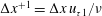
 $\unicode[STIX]{x0394}t$
is the transient period between the start of the valve opening and the time when the flow has reached 90 % of the final flow rate; and
$\unicode[STIX]{x0394}t$
is the transient period between the start of the valve opening and the time when the flow has reached 90 % of the final flow rate; and $t_{cr}$
is the critical time for the onset of transition, defined here as the time when the friction factor reaches a minimum.
$t_{cr}$
is the critical time for the onset of transition, defined here as the time when the friction factor reaches a minimum.

Simulation parameters used to reproduce the experimental flow cases. Here $\unicode[STIX]{x0394}x^{+1}=\unicode[STIX]{x0394}x\,u_{\unicode[STIX]{x1D70F}1}/\unicode[STIX]{x1D708}$
, where
$\unicode[STIX]{x0394}x^{+1}=\unicode[STIX]{x0394}x\,u_{\unicode[STIX]{x1D70F}1}/\unicode[STIX]{x1D708}$
, where $u_{\unicode[STIX]{x1D70F}1}$
is the friction velocity of the final flow and
$u_{\unicode[STIX]{x1D70F}1}$
is the friction velocity of the final flow and $\unicode[STIX]{x1D708}$
is the kinematic viscosity;
$\unicode[STIX]{x1D708}$
is the kinematic viscosity; $\unicode[STIX]{x0394}y_{c}^{+1}$
and
$\unicode[STIX]{x0394}y_{c}^{+1}$
and $\unicode[STIX]{x0394}z^{+1}$
are defined in a similar manner, and the subscript
$\unicode[STIX]{x0394}z^{+1}$
are defined in a similar manner, and the subscript $c$
refers to the centreline.
$c$
refers to the centreline.
Time histories of bulk velocity (Reynolds number) and friction coefficient ( $C_{f}$
) for case A2. The bulk velocity (markers) is obtained from integration of velocity profiles measured with PIV. Its time history is curve-fitted as a polynomial (line) for use as input in the LES simulation. The friction coefficient is defined as
$C_{f}$
) for case A2. The bulk velocity (markers) is obtained from integration of velocity profiles measured with PIV. Its time history is curve-fitted as a polynomial (line) for use as input in the LES simulation. The friction coefficient is defined as $C_{f}=\unicode[STIX]{x1D70F}_{w}/(0.5\unicode[STIX]{x1D70C}U_{b}^{2})$
, where
$C_{f}=\unicode[STIX]{x1D70F}_{w}/(0.5\unicode[STIX]{x1D70C}U_{b}^{2})$
, where $\unicode[STIX]{x1D70F}_{w}$
is wall shear stress,
$\unicode[STIX]{x1D70F}_{w}$
is wall shear stress, $\unicode[STIX]{x1D70C}$
the density of the fluid and
$\unicode[STIX]{x1D70C}$
the density of the fluid and $U_{b}$
the instantaneous bulk velocity.
$U_{b}$
the instantaneous bulk velocity.

LES have been carried out for comparison with selected experiments. Also, a DNS has been performed for one case with a low final Reynolds number for direct comparison with experiment and for validation of the LES calculation. The prescribed flow histories used in the LES and DNS simulations were obtained by curve-fitting the measured flow history. The simulations were performed using an in-house code, CHAPSim (Seddighi Reference Seddighi2011; He & Seddighi Reference He and Seddighi2013). The momentum and continuity equations are spatially discretised using a second-order, central finite-difference scheme. An explicit third-order Runge–Kutta scheme is used for temporal discretisation of the nonlinear terms, and an implicit second-order Crank–Nicolson scheme is used for the viscous terms. In addition, the continuity equation is enforced using the fractional-step method. The Poisson equation for the pressure is solved by an efficient two-dimensional fast Fourier transform solver. Periodic boundary conditions are applied in the streamwise and spanwise directions and a no-slip boundary condition is imposed on the top and bottom walls. Subgrid-scale stresses are modelled using the wall-adapting local eddy-viscosity (WALE) model of Nicoud & Ducros (Reference Nicoud and Ducros1999). The code validation can be found in Seddighi (Reference Seddighi2011), He & Seddighi (Reference He and Seddighi2013) and Mathur (Reference Mathur2016).
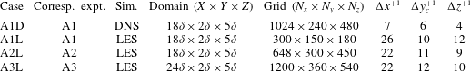
The key parameters of the simulations are shown in table 2. The computational mesh is uniform in the streamwise ( $x$
) and spanwise (
$x$
) and spanwise ( $z$
) directions, but non-uniform in the wall-normal (
$z$
) directions, but non-uniform in the wall-normal ( $y$
) direction. The resolution of the mesh of the LES simulations in the wall-normal direction was set to very close to that of the DNS, whereas the resolution in the other two directions was approximately three times coarser, thereby significantly reducing grid numbers but nevertheless maintaining good accuracy. As shown below in § 3, LES and DNS results for case A1 practically overlap each other; and the LES results and the experimental data agree closely for all cases and consistently show the same trends. Accordingly, the following discussion does not distinguish between the experimental and numerical results unless otherwise stated.
$y$
) direction. The resolution of the mesh of the LES simulations in the wall-normal direction was set to very close to that of the DNS, whereas the resolution in the other two directions was approximately three times coarser, thereby significantly reducing grid numbers but nevertheless maintaining good accuracy. As shown below in § 3, LES and DNS results for case A1 practically overlap each other; and the LES results and the experimental data agree closely for all cases and consistently show the same trends. Accordingly, the following discussion does not distinguish between the experimental and numerical results unless otherwise stated.
3 Results and discussion
Figure 2 shows a typical case (A2) with flow accelerating from $0.11~\text{m}~\text{s}^{-1}$
to
$0.11~\text{m}~\text{s}^{-1}$
to $0.60~\text{m}~\text{s}^{-1}$
in 1.9 s, or
$0.60~\text{m}~\text{s}^{-1}$
in 1.9 s, or $Re=2760$
to 15 200 in
$Re=2760$
to 15 200 in $t^{\ast }=8.3$
, where
$t^{\ast }=8.3$
, where $t^{\ast }=tU_{b0}/\unicode[STIX]{x1D6FF}$
, and
$t^{\ast }=tU_{b0}/\unicode[STIX]{x1D6FF}$
, and $U_{b0}$
is the bulk velocity of the initial flow. Immediately after the acceleration commences, the wall friction increases sharply to a peak value, as the viscous force on the wall restricts the acceleration of the fluid adjacent to it, causing a layer of high strain rate close to the wall. This new boundary layer then thickens by diffusion and the wall friction reduces. This trend continues until
$U_{b0}$
is the bulk velocity of the initial flow. Immediately after the acceleration commences, the wall friction increases sharply to a peak value, as the viscous force on the wall restricts the acceleration of the fluid adjacent to it, causing a layer of high strain rate close to the wall. This new boundary layer then thickens by diffusion and the wall friction reduces. This trend continues until $t\approx 2$
s, when the wall friction begins to increase again, reaching its final value at
$t\approx 2$
s, when the wall friction begins to increase again, reaching its final value at $t\approx 3$
s. Conventionally, the variation in the friction during the first period (up to 2 s) is associated with a period of frozen turbulence and the subsequent recovery is interpreted as a delayed but rapid response of turbulence (He et al.
Reference He, Ariyaratne and Vardy2011). As discussed in the rest of this paper, our new interpretation is that the recovery of the wall friction beginning at
$t\approx 3$
s. Conventionally, the variation in the friction during the first period (up to 2 s) is associated with a period of frozen turbulence and the subsequent recovery is interpreted as a delayed but rapid response of turbulence (He et al.
Reference He, Ariyaratne and Vardy2011). As discussed in the rest of this paper, our new interpretation is that the recovery of the wall friction beginning at $t\approx 2$
s is actually caused by the transition of the new temporally developing boundary layer formed alongside the wall. This boundary layer is initially laminar, but it gradually reaches a stage at which it is unstable and transition to turbulence occurs. It is shown below with flow visualisation that the minimum point of the friction factor
$t\approx 2$
s is actually caused by the transition of the new temporally developing boundary layer formed alongside the wall. This boundary layer is initially laminar, but it gradually reaches a stage at which it is unstable and transition to turbulence occurs. It is shown below with flow visualisation that the minimum point of the friction factor $C_{f}$
coincides with the onset of transition (
$C_{f}$
coincides with the onset of transition ( $t\approx 2$
s) and that the first peak in
$t\approx 2$
s) and that the first peak in $C_{f}$
after this coincides with the completion of the transition (
$C_{f}$
after this coincides with the completion of the transition ( $t\approx 3$
s). Consequently, the transient-flow transition can be divided into pre-transitional (
$t\approx 3$
s). Consequently, the transient-flow transition can be divided into pre-transitional ( $0\sim 2$
s), transitional (
$0\sim 2$
s), transitional ( $2\sim 3$
s) and fully turbulent phases (
$2\sim 3$
s) and fully turbulent phases ( ${>}3$
s).
${>}3$
s).
Distribution of the streamwise fluctuating velocity $u^{\prime }$
(
$u^{\prime }$
( $\text{m}~\text{s}^{-1}$
) over a horizontal plane close to the wall (
$\text{m}~\text{s}^{-1}$
) over a horizontal plane close to the wall ( $y=2~\text{mm}$
,
$y=2~\text{mm}$
, $y^{+0}=15$
, where
$y^{+0}=15$
, where $y^{+0}=yu_{\unicode[STIX]{x1D70F}0}/\unicode[STIX]{x1D708}$
with
$y^{+0}=yu_{\unicode[STIX]{x1D70F}0}/\unicode[STIX]{x1D708}$
with $y$
being the distance from the wall and
$y$
being the distance from the wall and $u_{\unicode[STIX]{x1D70F}0}$
the friction velocity of the initial flow) at several instants of the transient flow of case A2. The PIV measurements are on the left and the LES results are on the right.
$u_{\unicode[STIX]{x1D70F}0}$
the friction velocity of the initial flow) at several instants of the transient flow of case A2. The PIV measurements are on the left and the LES results are on the right.

3.1 Visualisation
The transition process is visualised in figure 3, which shows contours of the streamwise fluctuating velocity in a horizontal plane close to the wall obtained from PIV measurements and LES. The measurement area of the experiments is smaller than the LES computational domain, but the results essentially show the same flow development. At $t=0$
s, the flow shows random fluctuations with some weak streaky structures, a typical characteristic of turbulent flow at low Reynolds number. During the first stage (up to 2 s), high- and low-speed streaks are formed and these strengthen with time. This is a typical feature of the initial stage of boundary layer bypass transition (Jacobs & Durbin Reference Jacobs and Durbin2001; Matsubara & Alfredsson Reference Matsubara and Alfredsson2001), explained using the transient growth theory associated with lift-up processes (Landahl Reference Landahl1975; Trefethen et al.
Reference Trefethen, Trefethen, Reddy and Driscoll1993; Andersson et al.
Reference Andersson, Berggren and Henningson1999). After
$t=0$
s, the flow shows random fluctuations with some weak streaky structures, a typical characteristic of turbulent flow at low Reynolds number. During the first stage (up to 2 s), high- and low-speed streaks are formed and these strengthen with time. This is a typical feature of the initial stage of boundary layer bypass transition (Jacobs & Durbin Reference Jacobs and Durbin2001; Matsubara & Alfredsson Reference Matsubara and Alfredsson2001), explained using the transient growth theory associated with lift-up processes (Landahl Reference Landahl1975; Trefethen et al.
Reference Trefethen, Trefethen, Reddy and Driscoll1993; Andersson et al.
Reference Andersson, Berggren and Henningson1999). After $t=2$
s, isolated turbulent spots are generated locally and grow during the transition period (2 s to 3 s), eventually filling the entire wall surface. The transition is then complete.
$t=2$
s, isolated turbulent spots are generated locally and grow during the transition period (2 s to 3 s), eventually filling the entire wall surface. The transition is then complete.
Figure 4 illustrates the transition by means of time histories of the fluctuating velocities at all points on a line across the channel. During the pre-transitional phase, the wall-normal and the spanwise (not shown) fluctuating velocities remain completely calm and non-responding. Following the onset of transition at $t\approx 2$
s, strong responses begin spontaneously across the span of the channel during the transition period. Except that occasional isolated turbulent spots can be seen passing the monitoring line, the flow state switches abruptly, not gradually. This behaviour is in stark contrast to that of the streamwise fluctuating velocity (
$t\approx 2$
s, strong responses begin spontaneously across the span of the channel during the transition period. Except that occasional isolated turbulent spots can be seen passing the monitoring line, the flow state switches abruptly, not gradually. This behaviour is in stark contrast to that of the streamwise fluctuating velocity ( $u^{\prime }$
), which exhibits strong growth until the onset of transition, reflecting streaks passing the monitoring line. The transition exhibits itself here as discontinuities in both temporal and spatial scales of the flow structures before and after its occurrence.
$u^{\prime }$
), which exhibits strong growth until the onset of transition, reflecting streaks passing the monitoring line. The transition exhibits itself here as discontinuities in both temporal and spatial scales of the flow structures before and after its occurrence.
Time histories of the streamwise (a) and wall-normal (b) fluctuating velocities along a horizontal line across the span of the channel at $y=2$
mm based on LES.
$y=2$
mm based on LES.

The observed transition process closely resembles the character of transition predicted by DNS of rapid flow change under uniform acceleration from an initially steady turbulent flow (He & Seddighi Reference He and Seddighi2013). Unlike the numerically simulated flow, the simple valve opening operation in the present experiment results in a non-uniform acceleration with irregular oscillations (appendix B) and pressure waves. No special effort was made to limit such disturbances, or to reduce system vibrations generated by the pump. As a consequence, the close similarity between the numerical and experimental results is a clear indication that the transition process is robust and is insensitive to external disturbances. Furthermore, together with previous DNS studies (He & Seddighi Reference He and Seddighi2013, Reference He and Seddighi2015; Seddighi et al. Reference Seddighi, He, Vardy and Orlandi2014), the results imply that the transition behaviour is universally characteristic of transient flows of this kind.
At first sight, the laminar–turbulent transition observed here might appear almost inconceivable given that the initial flow is already turbulent. However, a simple resolution of this apparent paradox can be achieved by a change of perception of the observer. The transient flow following the opening of a valve is conventionally viewed as turbulent flow because of its initial state, and the behaviour is explained as a development of the pre-existing turbulence in the flow as it responds to the flow acceleration. The transition theory is based on the understanding that the transient flow following the opening of a valve is no longer the initial flow on its own, but one consisting of the initial turbulent flow and a new temporally developing boundary layer formed on the wall. As observed above and discussed in He & Seddighi (Reference He and Seddighi2013, Reference He and Seddighi2015) for a near-step increase flow, the dominant behaviour of the transient flow is a consequence of the development of the boundary layer, that is, its growth with time, the instabilities that it exhibits and the eventual breakdown to turbulence, reflecting a typical transitional process. In this interpretation, the pre-existing turbulent fluctuations act primarily as noise or disturbances, and their evolution can largely be related to the influence of the development of the boundary layer: outside the new boundary layer, the fluctuations evolve relatively freely, but inside it, they are significantly modulated by the new flow and this is the main cause of the elongated streaks. Thus, although the initial turbulence might be instrumental to the eventual transition, it is not, in itself, the defining feature of the flow.
In the following, we examine the development of the boundary layer, directly comparing it with a transient laminar flow experiment initiated from rest as well as a laminar flow solution. This is followed by a discussion on the development of turbulence statistics.
3.2 Temporally developing boundary layer
To characterise the development of the boundary layer during the pre-transitional phase, we examine the wall-normal profile of the perturbation velocity, defined here as the excess of the ensemble average velocity at time $t$
over the pre-existing steady flow velocity at time
$t$
over the pre-existing steady flow velocity at time $t=0~\text{s}$
when the acceleration begins. In non-dimensional form,
$t=0~\text{s}$
when the acceleration begins. In non-dimensional form,
 $$\begin{eqnarray}\displaystyle U^{\wedge }(y,t)=[U(y,t)-U(y,0)]/[U_{c}(t)-U_{c}(0)], & & \displaystyle\end{eqnarray}$$
where $U(y,t)$
is the mean velocity at time
$U(y,t)$
is the mean velocity at time $t$
and
$t$
and $U_{c}(t)$
is the velocity at the centre of the channel. This perturbation can be compared with a laminar transient flow undergoing the same variation in flow rate as shown in figure 2 but starting from rest. Such an experiment was carried out and is referred to as case L1. Theoretically, this laminar flow is described by the solution of an extended Stokes first problem (Schlichting & Gersten Reference Schlichting and Gersten2003)
$U_{c}(t)$
is the velocity at the centre of the channel. This perturbation can be compared with a laminar transient flow undergoing the same variation in flow rate as shown in figure 2 but starting from rest. Such an experiment was carried out and is referred to as case L1. Theoretically, this laminar flow is described by the solution of an extended Stokes first problem (Schlichting & Gersten Reference Schlichting and Gersten2003)
 $$\begin{eqnarray}\displaystyle U(y,t)=\int _{0}^{t}U_{b}^{\prime }(\unicode[STIX]{x1D70F})\,\text{erfc}\left(\frac{y}{2\sqrt{\unicode[STIX]{x1D708}(t-\unicode[STIX]{x1D70F})}}\right)\,\text{d}\unicode[STIX]{x1D70F}, & & \displaystyle\end{eqnarray}$$
where erfc is the complementary error function and $U_{b}^{\prime }(t)$
the bulk flow acceleration. Figure 5 shows that the boundary layer development of experiment A2 and the corresponding LES simulation, A2L, agree well with each other throughout the time presented, before and after the transition. Similarly, the Stokes solution and the transient laminar flow of comparable acceleration starting from rest (experiment case L1) almost collapse on top of each other. All four sets of data agree strikingly well until the onset of transition (
$U_{b}^{\prime }(t)$
the bulk flow acceleration. Figure 5 shows that the boundary layer development of experiment A2 and the corresponding LES simulation, A2L, agree well with each other throughout the time presented, before and after the transition. Similarly, the Stokes solution and the transient laminar flow of comparable acceleration starting from rest (experiment case L1) almost collapse on top of each other. All four sets of data agree strikingly well until the onset of transition ( $t\approx 2$
s), after which the laminar boundary layer (L1 and extended Stokes) continues to grow away from the wall, whereas the ‘turbulent’ cases (A2 and A2L) show a reduced boundary layer thickness following transition to turbulence. Figure 5 thus demonstrates that the transient turbulent flow initially behaves closely like an accelerating laminar flow superimposed on a steady turbulent flow.
$t\approx 2$
s), after which the laminar boundary layer (L1 and extended Stokes) continues to grow away from the wall, whereas the ‘turbulent’ cases (A2 and A2L) show a reduced boundary layer thickness following transition to turbulence. Figure 5 thus demonstrates that the transient turbulent flow initially behaves closely like an accelerating laminar flow superimposed on a steady turbulent flow.
Profiles of the perturbation velocity ( $U^{\wedge }$
) at various times for case A2. Expt-A2 and Expt-L1 are experimental data from tests starting from a turbulent flow and from rest, respectively; LES-A2L is LES simulation of A2; extended Stokes is solution of the extended Stokes first problem for a flow history of A2 with the initial flow subtracted.
$U^{\wedge }$
) at various times for case A2. Expt-A2 and Expt-L1 are experimental data from tests starting from a turbulent flow and from rest, respectively; LES-A2L is LES simulation of A2; extended Stokes is solution of the extended Stokes first problem for a flow history of A2 with the initial flow subtracted.

Development of the momentum Reynolds number of the temporally developing boundary layer represented by the perturbation velocity $U^{\wedge }$
with the equivalent Reynolds number – comparison between experiments, LES and extended Stokes solution, the latter being relevant only before transition.
$U^{\wedge }$
with the equivalent Reynolds number – comparison between experiments, LES and extended Stokes solution, the latter being relevant only before transition.

Figure 6 shows the transient growth of the momentum Reynolds number, $Re_{\unicode[STIX]{x1D703}}(t)=U_{b}(t)\unicode[STIX]{x1D703}(t)/\unicode[STIX]{x1D708}$
, where
$Re_{\unicode[STIX]{x1D703}}(t)=U_{b}(t)\unicode[STIX]{x1D703}(t)/\unicode[STIX]{x1D708}$
, where $\unicode[STIX]{x1D703}(t)=\int _{0}^{\infty }U^{\wedge }(y,t)(1-U^{\wedge }(y,t))\,\text{d}y$
, with respect to an equivalent Reynolds number based on a characteristic distance for three cases obtained from experiments, LES and the extended Stokes solution. For the temporally developing boundary layer considered here, we define the equivalent Reynolds number
$\unicode[STIX]{x1D703}(t)=\int _{0}^{\infty }U^{\wedge }(y,t)(1-U^{\wedge }(y,t))\,\text{d}y$
, with respect to an equivalent Reynolds number based on a characteristic distance for three cases obtained from experiments, LES and the extended Stokes solution. For the temporally developing boundary layer considered here, we define the equivalent Reynolds number $Re_{t}=x(t)U_{b}(t)/\unicode[STIX]{x1D708}$
, where
$Re_{t}=x(t)U_{b}(t)/\unicode[STIX]{x1D708}$
, where $x(t)$
is a convective distance. Because the flow accelerates in a gradual manner, the characteristic length is written as
$x(t)$
is a convective distance. Because the flow accelerates in a gradual manner, the characteristic length is written as $x(t)=\int _{0}^{t}U_{b}(\unicode[STIX]{x1D70F})\,\text{d}\unicode[STIX]{x1D70F}$
. It can be seen from figure 6 that the experimental and LES results agree closely during the pre-transition and transition periods, but they deviate from each other after the overall flow becomes fully turbulent. The discrepancy is explainable by the fact that the boundary layer is much thinner after the flow has become turbulent and, as a result, the experimental measurements are too coarse to resolve the boundary layer (see figure 4). The most significant observation from this figure is that the experiment and LES agree closely with the extended Stokes solutions during the early stages of flow in all three cases shown, again demonstrating that the initial flow development is of a laminar nature. At a later stage, the data deviate from the laminar solution at a point coincident with the onset of transition. The transitional Reynolds number marking this point increases from A1 to A2 to A3, which is discussed in § 3.4. Incidentally it is noted that the growths of the momentum Reynolds number with
$x(t)=\int _{0}^{t}U_{b}(\unicode[STIX]{x1D70F})\,\text{d}\unicode[STIX]{x1D70F}$
. It can be seen from figure 6 that the experimental and LES results agree closely during the pre-transition and transition periods, but they deviate from each other after the overall flow becomes fully turbulent. The discrepancy is explainable by the fact that the boundary layer is much thinner after the flow has become turbulent and, as a result, the experimental measurements are too coarse to resolve the boundary layer (see figure 4). The most significant observation from this figure is that the experiment and LES agree closely with the extended Stokes solutions during the early stages of flow in all three cases shown, again demonstrating that the initial flow development is of a laminar nature. At a later stage, the data deviate from the laminar solution at a point coincident with the onset of transition. The transitional Reynolds number marking this point increases from A1 to A2 to A3, which is discussed in § 3.4. Incidentally it is noted that the growths of the momentum Reynolds number with $Re_{t}$
calculated from the extended Stokes solutions are almost indistinguishable in the three cases.
$Re_{t}$
calculated from the extended Stokes solutions are almost indistinguishable in the three cases.
At this point, we revisit figure 2 in which the friction factor $C_{f}$
is shown. The theoretical prediction (marked Ext. Stokes) is based on the sum of the wall shear stress obtained from the extended Stokes first problem solution of the perturbation flow (
$C_{f}$
is shown. The theoretical prediction (marked Ext. Stokes) is based on the sum of the wall shear stress obtained from the extended Stokes first problem solution of the perturbation flow ( $U^{\wedge }$
) and that of the initial turbulent flow. It is clear from figure 2 that the prediction is in good agreement with the experimental and LES data for the entire period of pre-transition.
$U^{\wedge }$
) and that of the initial turbulent flow. It is clear from figure 2 that the prediction is in good agreement with the experimental and LES data for the entire period of pre-transition.
Transient development of mean velocity and the Reynolds stresses for experiment (A2) and LES (A2L). Symbols denote the experimental data; lines represent the LES results of A2L. All four panels share the same legend.

3.3 Turbulence statistics
Figure 7 shows the transient development of the mean velocity ( $U$
) and turbulent stresses (
$U$
) and turbulent stresses ( $u_{rms}^{\prime }$
,
$u_{rms}^{\prime }$
, $v_{rms}^{\prime }$
and
$v_{rms}^{\prime }$
and $\langle u^{\prime }v^{\prime }\rangle$
) with time for case A2 obtained from experiment and from LES. Figure 8 shows, for a number of cases, the increase of
$\langle u^{\prime }v^{\prime }\rangle$
) with time for case A2 obtained from experiment and from LES. Figure 8 shows, for a number of cases, the increase of $u_{rms}^{\prime }$
and
$u_{rms}^{\prime }$
and $v_{rms}^{\prime }$
during the early stages of the flow transient expressed in terms of profiles of
$v_{rms}^{\prime }$
during the early stages of the flow transient expressed in terms of profiles of $u_{rms}^{\prime \wedge }~(=(u_{rms}^{\prime }-u_{rms,0}^{\prime })/(U_{b1}-U_{b0}))$
, where subscripts 0 and 1 represent conditions at the start and end of the transient, and
$u_{rms}^{\prime \wedge }~(=(u_{rms}^{\prime }-u_{rms,0}^{\prime })/(U_{b1}-U_{b0}))$
, where subscripts 0 and 1 represent conditions at the start and end of the transient, and $v_{rms}^{\prime \wedge }$
is defined similarly. These are shown with respect to
$v_{rms}^{\prime \wedge }$
is defined similarly. These are shown with respect to $y^{+0}$
at regular intervals of
$y^{+0}$
at regular intervals of $t^{+0}$
, where
$t^{+0}$
, where $y^{+0}=u_{\unicode[STIX]{x1D70F},0}y/\unicode[STIX]{x1D708}$
,
$y^{+0}=u_{\unicode[STIX]{x1D70F},0}y/\unicode[STIX]{x1D708}$
, $t^{+0}=tu_{\unicode[STIX]{x1D70F},0}^{2}/\unicode[STIX]{x1D708}$
and
$t^{+0}=tu_{\unicode[STIX]{x1D70F},0}^{2}/\unicode[STIX]{x1D708}$
and $u_{\unicode[STIX]{x1D70F},0}$
is the friction velocity of the initial flow. Such a format of presentation was used by He & Seddighi (Reference He and Seddighi2015) for step-increase flows taking advantage of the facts that (1) the critical time
$u_{\unicode[STIX]{x1D70F},0}$
is the friction velocity of the initial flow. Such a format of presentation was used by He & Seddighi (Reference He and Seddighi2015) for step-increase flows taking advantage of the facts that (1) the critical time $t_{cr}^{+0}$
varies only slightly for the different flow conditions and (2)
$t_{cr}^{+0}$
varies only slightly for the different flow conditions and (2) $u_{rms}^{\prime \wedge }$
and
$u_{rms}^{\prime \wedge }$
and $v_{rms}^{\prime \wedge }$
from different flows nearly overlap each other at the same
$v_{rms}^{\prime \wedge }$
from different flows nearly overlap each other at the same $t^{+0}$
. Here,
$t^{+0}$
. Here, $t_{cr}^{+0}$
takes values of 117, 103 and 90 for A1, A2 and A3, respectively. Before discussing the flow behaviours, it can be noted that the DNS and LES results for A1 are practically indistinguishable from each other, and that overall the LES and the experimental data agree very well and they show practically the same transient behaviour for all the quantities shown. This is particularly the case when the time scales of the responses are concerned (figure 7). A number of observations can now be made.
$t_{cr}^{+0}$
takes values of 117, 103 and 90 for A1, A2 and A3, respectively. Before discussing the flow behaviours, it can be noted that the DNS and LES results for A1 are practically indistinguishable from each other, and that overall the LES and the experimental data agree very well and they show practically the same transient behaviour for all the quantities shown. This is particularly the case when the time scales of the responses are concerned (figure 7). A number of observations can now be made.
Perturbations of turbulent stresses during the pre-transition period for selected cases: (a) streamwise component and (b) wall-normal component.

Firstly, it can be seen that the streamwise fluctuating velocity starts to increase soon after the commencement of the flow transient (figure 8
a). The response starts from a region close to the wall and gradually extends further away from the wall. Typically, it reaches a level close to its final steady values at the onset of transition (see figure 7
b). Comparing these statistical variations of $u^{\prime }$
with the visualisation (figures 3 and 4), it can be concluded that the strong increase in streamwise turbulent fluctuations are due to the formation, strengthening and elongation of streaks during the pre-transition phase.
$u^{\prime }$
with the visualisation (figures 3 and 4), it can be concluded that the strong increase in streamwise turbulent fluctuations are due to the formation, strengthening and elongation of streaks during the pre-transition phase.
Secondly, both figures 7(c) and 8(b) show that the wall-normal turbulence $v_{rms}^{\prime }$
remains almost unchanged throughout the pre-transition period in all cases shown. At the onset of transition, it responds spontaneously in a relatively large region close to the wall, approximately
$v_{rms}^{\prime }$
remains almost unchanged throughout the pre-transition period in all cases shown. At the onset of transition, it responds spontaneously in a relatively large region close to the wall, approximately $y^{+0}<40$
. This is consistent with the flow visualisation, hence linking the delayed, rapid response of
$y^{+0}<40$
. This is consistent with the flow visualisation, hence linking the delayed, rapid response of $v_{rms}^{\prime }$
to the generation of turbulent spots during transition.
$v_{rms}^{\prime }$
to the generation of turbulent spots during transition.
Thirdly, it can be seen that the transition to turbulence represented by the generation and merging of turbulent spots is limited to the near-wall region. Consider figures 4(b) and 7(c) for example; the transition has completed before $t=3$
s by which time
$t=3$
s by which time $v_{rms}^{\prime }$
approaches its final steady values at say
$v_{rms}^{\prime }$
approaches its final steady values at say $y^{+0}=12$
and
$y^{+0}=12$
and $40$
; however, at
$40$
; however, at $y^{+0}=80$
,
$y^{+0}=80$
, $v_{rms}^{\prime }$
is only starting to increase at
$v_{rms}^{\prime }$
is only starting to increase at $t=3$
s, and another second elapses before there is a strong response at the centre of the channel,
$t=3$
s, and another second elapses before there is a strong response at the centre of the channel, $y^{+0}=179$
.
$y^{+0}=179$
.
Finally, the turbulent shear stress follows a trend similar to that of $v_{rms}^{\prime }$
, significantly different from that of
$v_{rms}^{\prime }$
, significantly different from that of $u_{rms}^{\prime }$
. The spanwise turbulence (not shown) shows a trend similar to that of
$u_{rms}^{\prime }$
. The spanwise turbulence (not shown) shows a trend similar to that of $v_{rms}^{\prime }$
.
$v_{rms}^{\prime }$
.
3.4 Critical Reynolds number
The critical Reynolds number at which transition occurs is a key parameter characterising the transition process. In a spatially developing boundary layer, this has been found to depend on the free-stream turbulence (Andersson et al.
Reference Andersson, Berggren and Henningson1999; Brandt, Schlatter & Henningson Reference Brandt, Schlatter and Henningson2004; Fransson, Matsubara & Alfredsson Reference Fransson, Matsubara and Alfredsson2005; Ovchinnikov, Choudhari & Piomelli Reference Ovchinnikov, Choudhari and Piomelli2008). It is now shown that this is also true for a temporally developing boundary layer. Here, the critical time is chosen to be the time when $C_{f}$
reaches a minimum. The free-stream turbulence is expressed as the ratio of the peak value of the root mean square (r.m.s.) of fluctuating velocity of the initial flow,
$C_{f}$
reaches a minimum. The free-stream turbulence is expressed as the ratio of the peak value of the root mean square (r.m.s.) of fluctuating velocity of the initial flow, $(u_{rms,0}^{\prime })_{max}$
, over the bulk velocity of the flow at the critical time,
$(u_{rms,0}^{\prime })_{max}$
, over the bulk velocity of the flow at the critical time, $U_{b,cr}$
, namely,
$U_{b,cr}$
, namely, $Tu_{0}=(u_{rms,0}^{\prime })_{max}/U_{b,cr}$
. If desired, turbulence quantities at other locations, such as at the centre of the channel, could be used instead of the peak values, but this would not change the conclusions, since the values are approximately proportional to each other.
$Tu_{0}=(u_{rms,0}^{\prime })_{max}/U_{b,cr}$
. If desired, turbulence quantities at other locations, such as at the centre of the channel, could be used instead of the peak values, but this would not change the conclusions, since the values are approximately proportional to each other.
Dependence of equivalent critical Reynolds number on turbulence intensity in various flow cases: experiments (A1–A7); the DNS and LES simulations of experiments (A1D, A1L–A3L); DNS simulations of the step-change flows (He & Seddighi Reference He and Seddighi2015); and best fit of experimental data (A1–A7), $Re_{t,cr}=2575Tu_{0}^{-1.52}$
. Inset: same data shown on logarithmic scale.
$Re_{t,cr}=2575Tu_{0}^{-1.52}$
. Inset: same data shown on logarithmic scale.

Figure 9 shows $Re_{t,cr}$
plotted against turbulence intensity
$Re_{t,cr}$
plotted against turbulence intensity $Tu_{0}$
for all experimental cases, LES and DNS results for selected cases and previous DNS simulations of step-change flows (He & Seddighi Reference He and Seddighi2015). The present data correlate closely and can be well represented by
$Tu_{0}$
for all experimental cases, LES and DNS results for selected cases and previous DNS simulations of step-change flows (He & Seddighi Reference He and Seddighi2015). The present data correlate closely and can be well represented by $Re_{t,cr}=2575Tu_{0}^{-1.52}$
. It has previously been shown that DNS data for step-change flows can be represented by
$Re_{t,cr}=2575Tu_{0}^{-1.52}$
. It has previously been shown that DNS data for step-change flows can be represented by $Re_{t,cr}\sim Tu_{0}^{-1.71}$
(He & Seddighi Reference He and Seddighi2015), whereas for a boundary layer the correlation is typically reported to have the form
$Re_{t,cr}\sim Tu_{0}^{-1.71}$
(He & Seddighi Reference He and Seddighi2015), whereas for a boundary layer the correlation is typically reported to have the form $Re_{cr}\sim Tu_{0}^{-2}$
(Westin et al.
Reference Westin, Boiko, Klingmann, Kozlov and Alfredsson1994; Andersson et al.
Reference Andersson, Berggren and Henningson1999). These results together show that the critical Reynolds number is closely related to the free-stream turbulence in each case, but the functional relationship may differ for different scenarios. Such functional differences are understandable considering the differences between the different groups of transitions. First we note a significant difference between the transient boundary layer flow and spatially developing boundary layers: the free-stream turbulence in a transient flow is wall shear turbulence that is strongly non-uniform and anisotropic; it decays relatively slowly outside the boundary layer. This contrasts with the homogeneous turbulence in the boundary layer flow, which decays rapidly with distance from the leading edge. Next, the difference between the step-increase flow of He & Seddighi (Reference He and Seddighi2015) and the present slower-accelerating flow is also apparent: the present flow is subjected to a variable free-stream velocity resulting in a complex boundary layer that can be described by the sum of small step changes in flow rate with delays in their starting times. This renders any representations of the free-stream velocity and convective distance (as used above in this paper) to be only nominal, not exactly equivalent to those of the step-change flows.
$Re_{cr}\sim Tu_{0}^{-2}$
(Westin et al.
Reference Westin, Boiko, Klingmann, Kozlov and Alfredsson1994; Andersson et al.
Reference Andersson, Berggren and Henningson1999). These results together show that the critical Reynolds number is closely related to the free-stream turbulence in each case, but the functional relationship may differ for different scenarios. Such functional differences are understandable considering the differences between the different groups of transitions. First we note a significant difference between the transient boundary layer flow and spatially developing boundary layers: the free-stream turbulence in a transient flow is wall shear turbulence that is strongly non-uniform and anisotropic; it decays relatively slowly outside the boundary layer. This contrasts with the homogeneous turbulence in the boundary layer flow, which decays rapidly with distance from the leading edge. Next, the difference between the step-increase flow of He & Seddighi (Reference He and Seddighi2015) and the present slower-accelerating flow is also apparent: the present flow is subjected to a variable free-stream velocity resulting in a complex boundary layer that can be described by the sum of small step changes in flow rate with delays in their starting times. This renders any representations of the free-stream velocity and convective distance (as used above in this paper) to be only nominal, not exactly equivalent to those of the step-change flows.
3.5 Discussion
We now briefly discuss the potential connection between the present work and the relaminarisation observed in spatially accelerating flows, including boundary layers subjected to strong FPG (e.g. Launder Reference Launder1964; Narasimha & Sreenivasan Reference Narasimha and Sreenivasan1979; Fernholz & Warnack Reference Fernholz and Warnack1998; Piomelli & Yuan Reference Piomelli and Yuan2013) and sink flows (e.g. Launder & Jones Reference Launder and Jones1969; Jones & Launder Reference Jones and Launder1972; Jones et al. Reference Jones, Marusic and Perry2001; Dixit & Ramesh Reference Dixit and Ramesh2008). Such flows are described to undergo a number of phases, namely, fully turbulent (I), reverse-transitional (II), quasi-laminar or relaminarised (III), and retransition to turbulence regions (IV) (Narasimha & Sreenivasan Reference Narasimha and Sreenivasan1973; Sreenivasan Reference Sreenivasan1982). At the stage of relaminarisation, the turbulence inherited from the initial flow is known not necessarily to reduce in absolute values in a major part of the flow, but the turbulent stresses become relatively unimportant in determining the mean flow dynamics in comparison to the strong acceleration (Sreenivasan Reference Sreenivasan1982).
Narasimha & Sreenivasan (Reference Narasimha and Sreenivasan1973) carried out a numerical analysis for a highly accelerated boundary layer by solving a laminar flow equation for the entire flow starting from the location when the acceleration began. This was done using a two-layer approach: the outer flow was treated as inviscid whereas the inner layer was laminar. This simple model reproduced the experimentally measured velocity profile really well everywhere from the start of the acceleration except very close to the wall. This rather surprisingly good result was understood to be due to the fact that the new boundary layer in the early stages of the flow (regions I and II) is thin and has little influence on the outer flow. For the velocity near the wall and the friction on the wall, the laminar model prediction agrees closely with experiments in the laminarised region (i.e. region III), whereas the fully turbulent model can approximate the behaviour reasonably well in region I. Region II remains less understood and less predictable.
Greenblatt & Moss (Reference Greenblatt and Moss1999) carried out a combined experimental and numerical study on a temporally accelerating flow. They identified laminarisation when the applied pressure gradient causing the temporal acceleration was similar to that for the spatially accelerating flow. Their numerical study included several alternative models and the wholly laminar ( $\overline{u^{\prime }v^{\prime }}=0$
) model, which corresponds broadly to the model of Narasimha & Sreenivasan (Reference Narasimha and Sreenivasan1973), was found to agree with the measured velocity profile closely, though no friction measurement was available for comparison.
$\overline{u^{\prime }v^{\prime }}=0$
) model, which corresponds broadly to the model of Narasimha & Sreenivasan (Reference Narasimha and Sreenivasan1973), was found to agree with the measured velocity profile closely, though no friction measurement was available for comparison.
The relaminarisation-based theory discussed above, in essence, describes a process of diminishing influence of turbulence and the quasi-laminar flow (region III) is a stage of the process when the effect of turbulence is negligible. In contrast, the transition-based viewpoint advocated here considers the transient flow to be characterised by a laminar-like boundary layer resulting from acceleration as soon as the flow is perturbed, and this is superimposed on the initial turbulent flow. This boundary layer dominates the development of the flow throughout the early stages of the flow.
The laminar models of Narasimha & Sreenivasan (Reference Narasimha and Sreenivasan1973) and Greenblatt & Moss (Reference Greenblatt and Moss1999) are different from that employed in the present work. In both of their models, the entire flow was assumed to be laminar as soon as the (spatial or temporal) acceleration started. Such a laminar model is for region III only and its application from the start of the acceleration was an approximation employed in the modelling for simplicity, not because it was stipulated by the theory. In the present extended Stokes analysis, the flow after commencement of acceleration is approximated as two independent components: (i) the original flow, which remains unchanged throughout the transient period until transition and (ii) a new laminar-like boundary layer, which develops near the wall in response to the flow acceleration. In practice, and in the theoretical framework, the initial turbulence and flow structure do not remain completely unchanged (e.g. formation of elongated streaks) and the two flow components are not completely independent. However, as shown in § 3.2, the present model seems to be able to predict the friction from the start of the acceleration for the temporally accelerating flow addressed here.
We note, however, that even though we expect some similarities between temporally accelerating flow and spatially accelerating flow and the above comparison may be of some interest to future studies, the spatial accelerating flow is more complex. Detailed analysis of the spatially accelerating flow is beyond the scope of the present paper.
4 Conclusions
In conclusion, we have observed that the transient flow starting from an already turbulent flow following the opening of a valve can be characterised closely by a temporally developing laminar boundary layer (superimposed by the slowly evolving pre-existing turbulence acting primarily as disturbances), and the transition of the boundary layer to turbulence. This is similar to that previously observed in a numerically simulated step-increase flow at low Reynolds numbers. The transition process is robust, not sensitive to the irregular flow acceleration and pressure waves present in the experiments; and the equivalent critical Reynolds number is uniquely related to the free-stream turbulence. Before transition, the development of the initially turbulent flow has been shown to be nearly identical to a laminar flow starting from rest. Both processes are described by the solution of the extended Stokes first problem of a laminar flow.
Acknowledgements
We gratefully acknowledge the contribution of Dr C. Ariyaratne at the early stage of the research and the advice provided by Professor P. Orlandi on numerical methods. Mr B. S. Oluwadare assisted with the experiments. The research was principally funded by EPSRC through grant EP/G068925/1. This work made use of computing facilities of the N8 HPC and ARCHER, funded by EPSRC through the N8 consortium (EP/K000225/1) and the UK Turbulence Consortium (EP/L000261/1), respectively. S.H., A.E.V., T.O’D. and D.P. initiated the research. S.G. designed the test rig, with contributions from all other authors, and conducted preliminary experiments. M.S. wrote the DNS code. A.M. together with M.S. implemented LES in the code. A.M. conducted the experiments and LES simulations. S.H., A.M., M.S. and S.G. analysed the results. S.H. led the writing of the manuscript, with contributions from all other authors. A.M. and S.G. made equal contributions.
Appendix A. Comparison of PIV measurement with benchmark data from literature
Comparison of outer-scaled experimental data with DNS data of Lee & Moser (Reference Lee and Moser2015) for steady channel flows at $Re=2800$
, 9800 and 20 100.
$Re=2800$
, 9800 and 20 100.

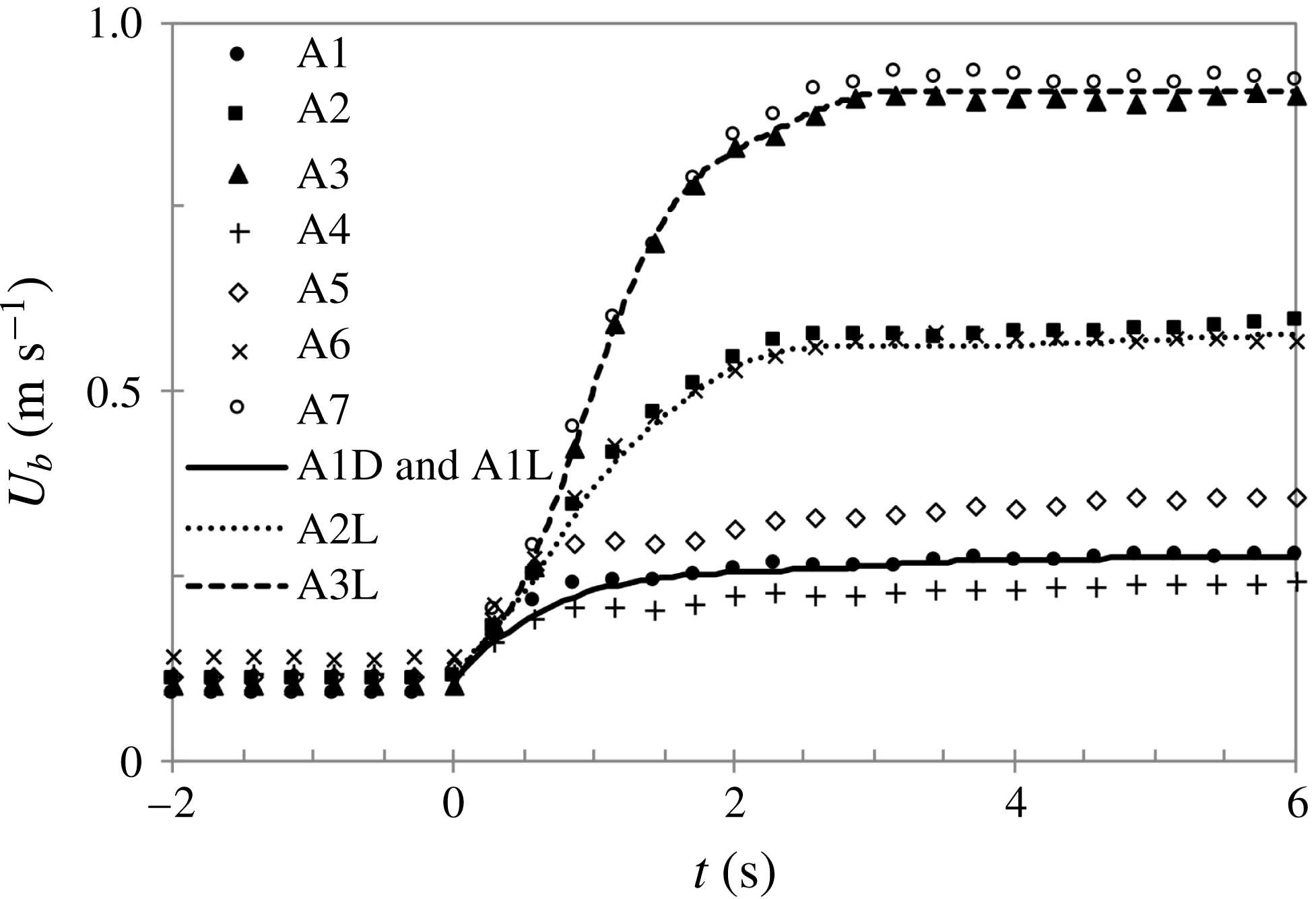
Variation of the bulk velocity obtained from integration of PIV velocity profiles for the experimental cases and curve fitting of the flow histories of A1–A3 that are used to specify flow variations for the LES and DNS simulations.
Experimentally measured profiles of the mean velocity and turbulent quantities of stationary turbulent flows for several Reynolds numbers are compared with the DNS benchmark data of Lee & Moser (Reference Lee and Moser2015) in figure 10. In the case of the mean velocity ( $U$
) and the r.m.s. of the streamwise velocity (
$U$
) and the r.m.s. of the streamwise velocity ( $u_{rms}^{\prime }$
), close agreement exists between the experimental data and the DNS results. Reasonably close agreement is also seen for the r.m.s. of the wall-normal fluctuating velocity (
$u_{rms}^{\prime }$
), close agreement exists between the experimental data and the DNS results. Reasonably close agreement is also seen for the r.m.s. of the wall-normal fluctuating velocity ( $v_{rms}^{\prime }$
) and the turbulent shear stress (
$v_{rms}^{\prime }$
) and the turbulent shear stress ( $-\langle u^{\prime }v^{\prime }\rangle$
), but the PIV measurements fail to capture the peaks of
$-\langle u^{\prime }v^{\prime }\rangle$
), but the PIV measurements fail to capture the peaks of $-\langle u^{\prime }v^{\prime }\rangle$
and
$-\langle u^{\prime }v^{\prime }\rangle$
and $v_{rms}^{\prime }$
near the wall. Also, somewhat larger discrepancies exist in
$v_{rms}^{\prime }$
near the wall. Also, somewhat larger discrepancies exist in $v_{rms}^{\prime }$
at low Reynolds number. These can be attributed to the use of a relatively large field of view in the PIV to capture the overall flow response (which limits the resolution) combined with a need to cover an unusually large velocity range (which necessitates a compromised PIV pulse frequency). Nevertheless, as shown in figure 7, these deficiencies do not impair the PIV system’s ability to capture the key features of the turbulent statistics of the transient flows.
$v_{rms}^{\prime }$
at low Reynolds number. These can be attributed to the use of a relatively large field of view in the PIV to capture the overall flow response (which limits the resolution) combined with a need to cover an unusually large velocity range (which necessitates a compromised PIV pulse frequency). Nevertheless, as shown in figure 7, these deficiencies do not impair the PIV system’s ability to capture the key features of the turbulent statistics of the transient flows.
Relative variation of the bulk velocity, $U_{b}^{\wedge }=(U_{b}(t)-U_{b0})/(U_{b1}-U_{b0})$
, in A2 and L1.
$U_{b}^{\wedge }=(U_{b}(t)-U_{b0})/(U_{b1}-U_{b0})$
, in A2 and L1. $U_{b0}=0~\text{m}~\text{s}^{-1}$
in L1.
$U_{b0}=0~\text{m}~\text{s}^{-1}$
in L1.

Appendix B. Detailed flow variations of transient experiments
Figure 11 shows the variation of the bulk velocity obtained by integrating PIV velocity profiles for the experimental cases and curve-fitting of the flow histories of A1 to A3 that are used to prescribe flow variations for the LES and DNS simulations.
Figure 12 shows the variation of the bulk velocity in a transient experiment undertaken for a flow initially at rest, i.e. the valve is initially fully closed. The result is based on a single run since the early flow is wholly laminar. There are some oscillations in the flow history because the valve opening from a fully closed position is difficult to control. Nevertheless, the overall relative flow variation agrees reasonably well with that of A2, thereby providing an opportunity for a direct comparison between the perturbation boundary layers in a laminar (L1) and a turbulent (A2) flow, e.g. figure 5.


 Open access