


1. Introduction
Practical combustion processes take place in a confined burner. As a consequence, internal combustion engines, gas turbines, etc. need to consider flame–wall interactions (FWIs). The presence of the wall not only significantly affects the flame dynamics (Ng et al. Reference Ng, Cheng, Robben and Talbot1982; Poinsot, Haworth & Bruneaux Reference Poinsot, Haworth and Bruneaux1993; Zhao, Wang & Chakraborty Reference Zhao, Wang and Chakraborty2018), but also influences pollutant production (Jiang et al. Reference Jiang, Brouzet, Talei, Gordon, Cazeres and Cuenot2021; Chi Reference Chi2024a ). Therefore, a comprehensive understanding of the near-wall flame dynamics is in great demand.
Due to the limited temporal and spatial resolutions in experiments and intricate near-wall turbulent flame dynamics, direct numerical simulation (DNS) appears as the most suitable approach to study the transient behaviour of the near-wall flame dynamics. Previous numerical studies on FWIs mostly focus on four different configurations as depicted in figure 1: (i) head-on quenching (Hocks, Peters & Adomeit Reference Hocks, Peters and Adomeit1981; Westbrook, Adamczyk & Lavoie Reference Westbrook, Adamczyk and Lavoie1981; Poinsot et al. Reference Poinsot, Haworth and Bruneaux1993; Wichman & Bruneaux Reference Wichman and Bruneaux1995; Bruneaux et al. Reference Bruneaux, Akselvoll, Poinsot and Ferziger1996; Popp, Smooke & Baum Reference Popp, Smooke and Baum1996; Bruneaux, Poinsot & Ferziger Reference Bruneaux, Poinsot and Ferziger1997; Popp & Baum Reference Popp and Baum1997; Ezekoye Reference Ezekoye1998; Dabireau et al. Reference Dabireau, Cuenot, Vermorel and Poinsot2003; Mari et al. Reference Mari, Cuenot, Rocchi, Selle and Duchaine2016; Sellmann et al. Reference Sellmann, Lai, Kempf and Chakraborty2017; Ohta, Onishi & Sakai Reference Ohta, Onishi and Sakai2022; Yu et al. Reference Yu, Cai, Chi, Mashruk, Valera-Medina and Maas2023; De Nardi et al. Reference De Nardi, Douasbin, Vermorel and Poinsot2024; Tamadonfar et al. Reference Tamadonfar, Karimkashi, Zirwes, Vuorinen and Kaario2024), (ii) side-wall quenching (Kármán & Millán Reference Kármán and Millán1953; Alshaalan & Rutland Reference Alshaalan and Rutland1998; Andrae et al. Reference Andrae, Björnbom, Edsberg and Eriksson2002; Gruber et al. Reference Gruber, Sankaran, Hawkes and Chen2010; Palulli, Talei & Gordon Reference Palulli, Talei and Gordon2019; Jiang et al. Reference Jiang, Brouzet, Talei, Gordon, Cazeres and Cuenot2021; Zhang et al. Reference Zhang, Zirwes, Häber, Bockhorn, Trimis and Suntz2021; Zirwes et al. Reference Zirwes2021; Kaddar et al. Reference Kaddar, Steinhausen, Zirwes, Bockhorn, Hasse and Ferraro2023; Luo et al. Reference Luo, Steinhausen, Kaddar, Hasse and Ferraro2023; Steinhausen et al. Reference Steinhausen, Zirwes, Ferraro, Scholtissek, Bockhorn and Hasse2023; Tamadonfar et al. Reference Tamadonfar, Salomaa, Rintanen, Karimkashi, Zirwes, Vuorinen and Kaario2025), (iii) tube quenching (Palmer & Tonkin Reference Palmer and Tonkin1963; Bai et al. Reference Bai, Chen, Zhang and Chen2013; Bioche, Vervisch & Ribert Reference Bioche, Vervisch and Ribert2018), and (iv) back-on quenching (Zhao et al. Reference Zhao, Wang and Chakraborty2018; Konstantinou, Ahmed & Chakraborty Reference Konstantinou, Ahmed and Chakraborty2021; Wang et al. Reference Wang, Wang, Luo, Hawkes, Chen and Fan2021; Zhao, Wang & Chakraborty Reference Zhao, Wang and Chakraborty2021; Zhao et al. Reference Zhao, Hernández, Francisco, Guo, Im and Wang2022, Reference Zhao, Zhang, Hernández Pérez, Im and Wang2023; Tomidokoro & Im Reference Tomidokoro and Im2024). In the present study we investigate the head-on flame quenching in a fully developed channel flow. This configuration was initially studied in Bruneaux et al. (Reference Bruneaux, Akselvoll, Poinsot and Ferziger1996, Reference Bruneaux, Poinsot and Ferziger1997) with one-step chemistry. Later, V-shaped premixed flames were studied in a channel flow in Alshaalan & Rutland (Reference Alshaalan and Rutland1998, Reference Alshaalan and Rutland2002), Gruber et al. (Reference Gruber, Sankaran, Hawkes and Chen2010), Wang & Tanahashi (Reference Wang and Tanahashi2024). Recently, both the head-on and V-shaped flames were studied and compared in a channel flow in Ahmed et al. (Reference Ahmed, Chakraborty and Klein2021b
,
Reference Ahmed, Chakraborty and Kleinc
,
Reference Ahmed, Chakraborty and Kleind
, Reference Ahmed, Chakraborty and Klein2023), Ghai et al. (Reference Ghai, Ahmed, Klein and Chakraborty2023). This configuration is interesting because the wall turbulence is statistically steady and can be uniquely described based on the friction Reynolds number Re $_\tau$
. More specifically, a turbulent boundary layer is typically present in practical systems, so that the conclusions are useful and instructive.
$_\tau$
. More specifically, a turbulent boundary layer is typically present in practical systems, so that the conclusions are useful and instructive.
Sketch of the four different FWI configurations.

Previous studies have revealed different physics for near-wall flames compared with free flames, due to wall confinement and wall heat loss. One of the most distinct observations is that the flame thickness would increase significantly near the wall (Gruber et al. Reference Gruber, Sankaran, Hawkes and Chen2010; Gruber et al. Reference Gruber, Richardson, Aditya and Chen2018; Zhao et al. Reference Zhao, Wang and Chakraborty2018). This would result in a change of the turbulent combustion regime for near-wall flames and directly affect the flame surface density (Bruneaux et al. Reference Bruneaux, Poinsot and Ferziger1997; Sellmann et al. Reference Sellmann, Lai, Kempf and Chakraborty2017). Gruber et al. (Reference Gruber, Sankaran, Hawkes and Chen2010) proposed two reasons to explain the increased flame thickness in their study: (i) the increased unsteadiness and wrinkling of the flame brush near the wall results in an increase of the averaged flame thickness, and (ii) the turbulent length and time scales decrease near the wall, while the chemical time scale increases due to heat loss. This results in a decrease in the local Damköhler number and entrainment of small eddies into the flame zone. These two reasons can be summarised as (i) effects of wall heat loss and (ii) near-wall change of turbulent scales. Though being physically perfectly reasonable, the two phenomena proposed in Gruber et al. (Reference Gruber, Sankaran, Hawkes and Chen2010) have to our knowledge never been fully validated. Additionally, variations of turbulent length and time scales near the wall were found to be highly dependent on the friction Reynolds number (Ahmed et al. Reference Ahmed, Apsley, Stallard, Stansby and Afgan2021a ), and it is not clear which one is the dominant factor for flame thickening during FWIs.
Apart from flame thickness, another distinct observation is that the flame displacement speed is still large even when the reaction rate becomes negligibly small and the global flame burning rate approaches zero as the flame is very close to the wall (Gruber et al. Reference Gruber, Sankaran, Hawkes and Chen2010; Zhao et al. Reference Zhao, Wang and Chakraborty2021, Reference Zhao, Hernández, Francisco, Guo, Im and Wang2022). Flame displacement speed is an important quantity to characterise the turbulent flame propagation speed and is essential for modelling turbulent premixed combustion (Dave & Chaudhuri Reference Dave and Chaudhuri2020). Very recently, Tomidokoro & Im (Reference Tomidokoro and Im2024) explained that the non-zero flame displacement speed near the wall is because of the diffusive term in the non-reactive region of the flame zone. This explanation is built on the back-on quenching configuration. However, this may not explain the similar behaviour observed in the head-on quenching configuration. Hence, further investigations of the flame displacement speed statistics in such configuration are needed.
Due to the change of flame thickness and flame speed near walls, the turbulent combustion regime would also change. Since the turbulence scales are also varying with wall distance, an accurate determination of the combustion regime during FWIs is difficult, but especially important for reduced models (Reynolds-averaged Navier–Stokes and large-eddy simulations), which are often designed for specific combustion regimes. Only few studies have been done to investigate the combustion regime dynamics during FWIs. Gruber et al. (Reference Gruber, Richardson, Aditya and Chen2018) investigated the combustion regime for premixed and stratified flames propagating in a turbulent channel flow and observed a transition from ‘thin flamelets’ in the bulk flow to ‘thickened flamelets’ near the wall. This is qualitatively consistent with the findings in Gruber et al. (Reference Gruber, Sankaran, Hawkes and Chen2010) (for side-wall quenching) and Zhao et al. (Reference Zhao, Wang and Chakraborty2018) (for back-on quenching). However, these studies did not investigate quantitatively at which wall distance the combustion regime is changing.
The main objectives of the present study are therefore to (i) quantify separately the effects of wall heat loss and wall turbulence on flame thickness during FWIs, (ii) analyse the dynamics of flame displacement speed and reveal the underlying reason for the high displacement speed very close to the wall, (iii) investigate the evolution of the turbulent combustion regime during FWIs, and (iv) clarify the cumulative effects of wall turbulence and wall heat loss on the turbulent flame dynamics during FWIs. To achieve these objectives, DNS of turbulent premixed H $_2/$
air and NH
$_2/$
air and NH $_3/$
H
$_3/$
H $_2/$
air flames in a fully developed channel flow at Re
$_2/$
air flames in a fully developed channel flow at Re $_\tau$ $\approx$
300 with both isothermal and adiabatic walls are carried out. These specific fuels have been selected since H
$\approx$
300 with both isothermal and adiabatic walls are carried out. These specific fuels have been selected since H $_2$
and NH
$_2$
and NH $_3/$
H
$_3/$
H $_2$
are attracting increasing attention in the combustion community due to their high energy efficiency while being carbon free (Valera-Medina et al. Reference Valera-Medina, Xiao, Owen-Jones, David and Bowen2018; Kobayashi et al. Reference Kobayashi, Hayakawa, Somarathne and Okafor2019; Pitsch Reference Pitsch2024). Thus, the present study is especially relevant for the upcoming energy transition and provides new physical insights on the FWI process for such flames. In what follows, § 2 introduces the numerical configurations, § 3 presents the results for a laminar FWI process, before the turbulent results are discussed and analysed in detail in § 4. The final conclusions are summarised in § 5.
$_2$
are attracting increasing attention in the combustion community due to their high energy efficiency while being carbon free (Valera-Medina et al. Reference Valera-Medina, Xiao, Owen-Jones, David and Bowen2018; Kobayashi et al. Reference Kobayashi, Hayakawa, Somarathne and Okafor2019; Pitsch Reference Pitsch2024). Thus, the present study is especially relevant for the upcoming energy transition and provides new physical insights on the FWI process for such flames. In what follows, § 2 introduces the numerical configurations, § 3 presents the results for a laminar FWI process, before the turbulent results are discussed and analysed in detail in § 4. The final conclusions are summarised in § 5.
2. Numerical configurations
The present study involves DNS of turbulent premixed H $_2/$
air and NH
$_2/$
air and NH $_3/$
H
$_3/$
H $_2/$
air flames in a fully developed channel flow. The case set-up is similar to our recent studies in (Chi et al. Reference Chi, Yu, Cuenot, Maas and Thévenin2024, Reference Chi, Theisel and Thévenin2023b
; Chi Reference Chi2024a
). The detailed mechanism from Jiang et al. (Reference Jiang, Gruber, Seshadri and Williams2020) has been used to simulate the NH
$_2/$
air flames in a fully developed channel flow. The case set-up is similar to our recent studies in (Chi et al. Reference Chi, Yu, Cuenot, Maas and Thévenin2024, Reference Chi, Theisel and Thévenin2023b
; Chi Reference Chi2024a
). The detailed mechanism from Jiang et al. (Reference Jiang, Gruber, Seshadri and Williams2020) has been used to simulate the NH $_3/$
H
$_3/$
H $_2/$
air combustion kinetics, after successful validation in previous investigations (Chi et al. Reference Chi, Han and Thévenin2023a
; Chi & Thévenin Reference Chi and Thévenin2023). Regarding H
$_2/$
air combustion kinetics, after successful validation in previous investigations (Chi et al. Reference Chi, Han and Thévenin2023a
; Chi & Thévenin Reference Chi and Thévenin2023). Regarding H $_2/$
air combustion kinetics, the mechanism from Li et al. (Reference Li, Zhao, Kazakov and Dryer2004) has been used, as for the previous FWI study in Gruber et al. (Reference Gruber, Sankaran, Hawkes and Chen2010). A mixture-averaged diffusion model has been applied to describe molecular species transport. Soret effect (thermodiffusion) is not considered since this effect has been found negligible during the FWI process (Yu et al. Reference Yu, Cai, Chi, Mashruk, Valera-Medina and Maas2023). All the DNS are carried out using the in-house combustion solver DINO (Abdelsamie et al. Reference Abdelsamie, Fru, Oster, Dietzsch, Janiga and Thévenin2016).
$_2/$
air combustion kinetics, the mechanism from Li et al. (Reference Li, Zhao, Kazakov and Dryer2004) has been used, as for the previous FWI study in Gruber et al. (Reference Gruber, Sankaran, Hawkes and Chen2010). A mixture-averaged diffusion model has been applied to describe molecular species transport. Soret effect (thermodiffusion) is not considered since this effect has been found negligible during the FWI process (Yu et al. Reference Yu, Cai, Chi, Mashruk, Valera-Medina and Maas2023). All the DNS are carried out using the in-house combustion solver DINO (Abdelsamie et al. Reference Abdelsamie, Fru, Oster, Dietzsch, Janiga and Thévenin2016).
Cold channel flows are firstly simulated until the wall turbulence is fully developed. The channel has streamwise ( $x$
), wall-normal (
$x$
), wall-normal ( $y$
) and spanwise (
$y$
) and spanwise ( $z$
) lengths of
$z$
) lengths of $5h$
,
$5h$
, $2h$
and
$2h$
and $2h$
, respectively, where
$2h$
, respectively, where $h =5$
mm is the half-width of the channel. This domain size is large enough in both the streamwise and spanwise directions to capture all turbulence scales, as clarified in Appendix A. A detailed validation of the wall turbulence statistics of the cold flows can be found in Chi et al. (Reference Chi, Yu, Cuenot, Maas and Thévenin2024). Further validations of the cold flow concerning turbulent dissipation rate and turbulent kinetic energy distribution can be found in Appendix B. Afterwards, two identical flame fronts (mapped from one-dimensional (1-D) unstretched freely propagating flame solutions) are initiated at
$h =5$
mm is the half-width of the channel. This domain size is large enough in both the streamwise and spanwise directions to capture all turbulence scales, as clarified in Appendix A. A detailed validation of the wall turbulence statistics of the cold flows can be found in Chi et al. (Reference Chi, Yu, Cuenot, Maas and Thévenin2024). Further validations of the cold flow concerning turbulent dissipation rate and turbulent kinetic energy distribution can be found in Appendix B. Afterwards, two identical flame fronts (mapped from one-dimensional (1-D) unstretched freely propagating flame solutions) are initiated at $y = 0.5 h$
and
$y = 0.5 h$
and $y = 1.5 h$
, with burned gases in the channel centre and flames propagating towards the top and bottom cold walls, as shown in figure 2. The simulations are continued until the flames quench on the isothermal wall or consume all fresh gases near the adiabatic wall. In total, these DNS required nearly 15 million CPU hours on the supercomputer JUWELS in the Jülich Supercomputing Center Germany and produced 12 TB of data, which are freely shared on Zenodo (Chi Reference Chi2024b
). The numerical details are listed in table 1.
$y = 1.5 h$
, with burned gases in the channel centre and flames propagating towards the top and bottom cold walls, as shown in figure 2. The simulations are continued until the flames quench on the isothermal wall or consume all fresh gases near the adiabatic wall. In total, these DNS required nearly 15 million CPU hours on the supercomputer JUWELS in the Jülich Supercomputing Center Germany and produced 12 TB of data, which are freely shared on Zenodo (Chi Reference Chi2024b
). The numerical details are listed in table 1.
Direct numerical simulation configuration showing the propagation of the flame surfaces towards the top and bottom channel walls at different times (from top to bottom) for a H $_2/$
air flame (left, case HI) and a NH
$_2/$
air flame (left, case HI) and a NH $_3/$
H
$_3/$
H $_2/$
air flame (right, case AI). The flame surface is indicated by
$_2/$
air flame (right, case AI). The flame surface is indicated by $C = C^\ast =0.55$
in case HI and
$C = C^\ast =0.55$
in case HI and $C = C^\ast =0.78$
in case AI, with the progress variable
$C = C^\ast =0.78$
in case AI, with the progress variable $C$
defined by Y
$C$
defined by Y $_{{{\rm H}_2{\rm O}}}$
and
$_{{{\rm H}_2{\rm O}}}$
and $C^\ast$
corresponding to the peak of heat release rate (HRR) in the corresponding laminar flames. The flame surfaces have been coloured by the surface density function (SDF)
$C^\ast$
corresponding to the peak of heat release rate (HRR) in the corresponding laminar flames. The flame surfaces have been coloured by the surface density function (SDF) $|\boldsymbol{\nabla }C|$
.
$|\boldsymbol{\nabla }C|$
.

Numerical details of the DNS cases. Here ISO denotes isothermal and AD denotes adiabatic.

The table contains the viscous length scale $l^{\ast } = \nu /u_{\tau }$
, with
$l^{\ast } = \nu /u_{\tau }$
, with $\nu$
the kinematic viscosity, as well as the friction Reynolds number Re
$\nu$
the kinematic viscosity, as well as the friction Reynolds number Re $_{\tau }$
=
$_{\tau }$
= $hu_\tau /\nu$
and wall Damköhler number Da
$hu_\tau /\nu$
and wall Damköhler number Da $_w$
=
$_w$
= $t_w/t_L$
(Gruber et al. Reference Gruber, Sankaran, Hawkes and Chen2010). The quantity
$t_w/t_L$
(Gruber et al. Reference Gruber, Sankaran, Hawkes and Chen2010). The quantity $t_w = \nu /u_{\tau }^2$
is the wall time scale and
$t_w = \nu /u_{\tau }^2$
is the wall time scale and $t_L = \delta _L/S_L$
is the flame time scale, with
$t_L = \delta _L/S_L$
is the flame time scale, with $\delta _L = (T_{ad}-T_u)/\max (|\boldsymbol{\nabla }T|)$
the laminar flame thickness of the unstretched freely propagating laminar flame,
$\delta _L = (T_{ad}-T_u)/\max (|\boldsymbol{\nabla }T|)$
the laminar flame thickness of the unstretched freely propagating laminar flame, $T_{ad}$
and
$T_{ad}$
and $T_u$
the adiabatic flame temperature and unburned gas temperature, respectively. Here
$T_u$
the adiabatic flame temperature and unburned gas temperature, respectively. Here $S_L$
is the laminar flame speed. Selecting an equivalence ratio
$S_L$
is the laminar flame speed. Selecting an equivalence ratio $\phi = 1.5$
for the H
$\phi = 1.5$
for the H $_2/$
air flame reduces the potential effect of thermodiffusive instability and is consistent with the previous study in Gruber et al. (Reference Gruber, Sankaran, Hawkes and Chen2010). On the other hand, using
$_2/$
air flame reduces the potential effect of thermodiffusive instability and is consistent with the previous study in Gruber et al. (Reference Gruber, Sankaran, Hawkes and Chen2010). On the other hand, using $\phi = 1.0$
for the NH
$\phi = 1.0$
for the NH $_3/$
H
$_3/$
H $_2/$
air flame leads to a higher flame velocity (keeping in mind the typically very low flame speeds obtained when burning ammonia), resulting in a shorter channel transit time and lower computational cost. Overall, there are four DNS cases: case HI and case AI are H
$_2/$
air flame leads to a higher flame velocity (keeping in mind the typically very low flame speeds obtained when burning ammonia), resulting in a shorter channel transit time and lower computational cost. Overall, there are four DNS cases: case HI and case AI are H $_2/$
air and NH
$_2/$
air and NH $_3/$
H
$_3/$
H $_2/$
air flames with isothermal walls, while case HA and case AA are the same flames, but with adiabatic walls. Case HI and case HA are simulated with a grid resolution
$_2/$
air flames with isothermal walls, while case HA and case AA are the same flames, but with adiabatic walls. Case HI and case HA are simulated with a grid resolution $\Delta x^+$
= 2.71 (uniformly 48.4
$\Delta x^+$
= 2.71 (uniformly 48.4 $\unicode{x03BC}$
m),
$\unicode{x03BC}$
m), $\Delta z^+$
= 2.189 (uniformly 39.1
$\Delta z^+$
= 2.189 (uniformly 39.1 $\unicode{x03BC}$
m) and 0.437
$\unicode{x03BC}$
m) and 0.437 $\leqslant \Delta y^+ \leqslant$
1.635 (stretched grids in the wall-normal direction from 7.8–29.2
$\leqslant \Delta y^+ \leqslant$
1.635 (stretched grids in the wall-normal direction from 7.8–29.2 $\unicode{x03BC}$
m). Case AI and case AA are simulated with a grid resolution
$\unicode{x03BC}$
m). Case AI and case AA are simulated with a grid resolution $\Delta x^+$
= 2.023 (uniformly 32.3
$\Delta x^+$
= 2.023 (uniformly 32.3 $\unicode{x03BC}$
m),
$\unicode{x03BC}$
m), $\Delta z^+$
= 2.448 (uniformly 39.
$\Delta z^+$
= 2.448 (uniformly 39. $\unicode{x03BC}$
m) and 0.326
$\unicode{x03BC}$
m) and 0.326 $\leqslant \Delta y^+ \leqslant$
1.215 (stretched grids in the wall-normal direction from 5.2–19.4
$\leqslant \Delta y^+ \leqslant$
1.215 (stretched grids in the wall-normal direction from 5.2–19.4 $\unicode{x03BC}$
m). Both resolutions are fine enough to resolve all (wall-) turbulence length scales and flame length scales, with at least 13 grid points within the flame thickness during the FWI process.
$\unicode{x03BC}$
m). Both resolutions are fine enough to resolve all (wall-) turbulence length scales and flame length scales, with at least 13 grid points within the flame thickness during the FWI process.
Apart from the three-dimensional (3-D) turbulent cases, 1-D laminar cases are also simulated to check independently the effects of wall heat loss. The laminar cases are set up similar to the 3-D turbulent cases in the wall-normal ( $y$
) direction, with the same spatial distribution for the initial thermochemical states. Four laminar cases corresponding to those in table 1 are finally simulated, denoted as case HIL, case AIL, case HAL and case AAL in the following discussion.
$y$
) direction, with the same spatial distribution for the initial thermochemical states. Four laminar cases corresponding to those in table 1 are finally simulated, denoted as case HIL, case AIL, case HAL and case AAL in the following discussion.
3. Laminar FWI
To understand the effects of wall heat loss, we first analyse in detail the underlying mechanisms controlling flame thickness during laminar FWIs.
3.1. Definitions of flame thickness
There are different definitions for the flame thickness. It is important to distinguish the differences between those different definitions before the dynamics of flame thickness can be correctly captured during FWIs. In the present study, different definitions are evaluated and compared. Flame thickness can usually be defined based on the surface density function (SDF) $|\boldsymbol{\nabla }C|$
as
$|\boldsymbol{\nabla }C|$
as
 \begin{equation} \delta _{\!f} = \left (\frac {1}{|\boldsymbol{\nabla }C|}\right )_{\textit{iso}} \end{equation}
on a certain isosurface (3-D)/isoline (2-D)/point (1-D), where $C$
is the progress variable. If
$C$
is the progress variable. If $C$
is defined thermally,
$C$
is defined thermally,
 \begin{equation} C = C_{T}= \frac {T-T_u}{T_b-T_u}, \end{equation}
then $\delta _{\!f} = \delta _t$
is called thermal flame thickness. Here,
$\delta _{\!f} = \delta _t$
is called thermal flame thickness. Here, $T_b$
is the burned gas temperature, usually taken equal to
$T_b$
is the burned gas temperature, usually taken equal to $T_{ad}$
. On the other hand, if
$T_{ad}$
. On the other hand, if $C$
is defined chemically,
$C$
is defined chemically,
 \begin{equation} C = C_{k} = \frac {Y_k-Y_{k,u}}{Y_{k,b}-Y_{k,u}}, \end{equation}
then $\delta _{\!f} = \delta _c$
is called chemical flame thickness. Here,
$\delta _{\!f} = \delta _c$
is called chemical flame thickness. Here, $Y_{k,u}$
and
$Y_{k,u}$
and $Y_{k,b}$
are mass fractions of species
$Y_{k,b}$
are mass fractions of species $k$
in the unburned and burned gas, respectively. In the present study we have chosen Y
$k$
in the unburned and burned gas, respectively. In the present study we have chosen Y $_{{{\rm H}_2{\rm O}}}$
in (3.3) to define the chemical progress variable
$_{{{\rm H}_2{\rm O}}}$
in (3.3) to define the chemical progress variable $C_{k}$
. During the FWI process,
$C_{k}$
. During the FWI process, $T_u$
and
$T_u$
and $Y_{k,u}$
might change with time, especially for an adiabatic wall. To make this scale time-independent, we use the initial values of
$Y_{k,u}$
might change with time, especially for an adiabatic wall. To make this scale time-independent, we use the initial values of $T_u$
and
$T_u$
and $Y_{k,u}$
before flame quenching for the normalisation in (3.2) and (3.3). There are several ways to choose a value of
$Y_{k,u}$
before flame quenching for the normalisation in (3.2) and (3.3). There are several ways to choose a value of $C$
to calculate the flame thickness, these are as follows.
$C$
to calculate the flame thickness, these are as follows.
-
(i) Method 1: value of $C$
where the instantaneous peak heat release rate (HRR)/fuel consumption rate is found.
$C$
where the instantaneous peak heat release rate (HRR)/fuel consumption rate is found. -
(ii) Method 2:
$C = C^{\ast }$
,
$C^{\ast }$
being chosen where HRR reaches a peak value in the corresponding unstretched, freely propagating laminar flame. -
(iii) Method 3: value of
$C$
where the maximum gradient of
$C$
is located.


In principle, these three definitions are consistent for unstretched freely propagating laminar flames. However, during FWIs, there are obvious discrepancies between these definitions. Especially, the value of $C$
in method 1 is not constant any more during FWIs, as shown in figure 29 in Appendix C. In the present study, all these three choices are evaluated for both the thermal and chemical flame thickness, so that
$C$
in method 1 is not constant any more during FWIs, as shown in figure 29 in Appendix C. In the present study, all these three choices are evaluated for both the thermal and chemical flame thickness, so that $\delta _{c1}$
,
$\delta _{c1}$
, $\delta _{c2}$
and
$\delta _{c2}$
and $\delta _{c3}$
represent chemical flame thickness defined with method 1, 2 and 3, respectively, and
$\delta _{c3}$
represent chemical flame thickness defined with method 1, 2 and 3, respectively, and $\delta _{t1}$
,
$\delta _{t1}$
, $\delta _{t2}$
and
$\delta _{t2}$
and $\delta _{t3}$
represent thermal flame thickness defined with these same methods. In the following discussion, all the thicknesses are normalised by the laminar flame thickness
$\delta _{t3}$
represent thermal flame thickness defined with these same methods. In the following discussion, all the thicknesses are normalised by the laminar flame thickness $\delta _L$
, to become
$\delta _L$
, to become $\delta _k^{\ast }$
=
$\delta _k^{\ast }$
= $\delta _k/\delta _L$
(
$\delta _k/\delta _L$
( $k = c1,c2,\ldots ,t3$
).
$k = c1,c2,\ldots ,t3$
).
Figure 3 depicts the time evolution of $1/{\delta _k^{\ast }}$
during FWI in case HIL (figure 3
a) and case HAL (figure 3
b). The evolution of the Peclet number (denoted as Pe) is also shown. This quantity describes the normalised flame–wall distance as Pe =
$1/{\delta _k^{\ast }}$
during FWI in case HIL (figure 3
a) and case HAL (figure 3
b). The evolution of the Peclet number (denoted as Pe) is also shown. This quantity describes the normalised flame–wall distance as Pe = $d/\delta _z$
(Bruneaux et al. Reference Bruneaux, Akselvoll, Poinsot and Ferziger1996), with
$d/\delta _z$
(Bruneaux et al. Reference Bruneaux, Akselvoll, Poinsot and Ferziger1996), with $d$
the mean flame–wall distance and
$d$
the mean flame–wall distance and $\delta _z = \lambda _u/(\rho _uc_pS_L)$
the Zel’dovich flame thickness, where
$\delta _z = \lambda _u/(\rho _uc_pS_L)$
the Zel’dovich flame thickness, where $\lambda _u, \rho _u$
and
$\lambda _u, \rho _u$
and $c_p$
denote the thermal diffusion coefficient, density and heat capacity of the unburned mixture, respectively. As shown, the flame quenches at
$c_p$
denote the thermal diffusion coefficient, density and heat capacity of the unburned mixture, respectively. As shown, the flame quenches at $t\boldsymbol{\cdot }S_L/\delta _L \approx 13.45$
in case HIL and at
$t\boldsymbol{\cdot }S_L/\delta _L \approx 13.45$
in case HIL and at $t\boldsymbol{\cdot }S_L/\delta _L \approx 13.35$
in case HAL. All flame thicknesses begin to change shortly before the quenching time, apart from
$t\boldsymbol{\cdot }S_L/\delta _L \approx 13.35$
in case HAL. All flame thicknesses begin to change shortly before the quenching time, apart from $\delta _{t3}^\ast$
, which reacts much earlier. This is because the value of
$\delta _{t3}^\ast$
, which reacts much earlier. This is because the value of $\max |\boldsymbol{\nabla }T|$
is very sensitive to the near-wall temperature profile, which is affected much earlier than flame quenching, corresponding to a zone of influence much larger than the quenching zone (Poinsot et al. Reference Poinsot, Haworth and Bruneaux1993; Gruber et al. Reference Gruber, Sankaran, Hawkes and Chen2010; Zhao et al. Reference Zhao, Wang and Chakraborty2018). By inspecting the trends of flame thickness variation during FWIs, it can be observed that all chemical thicknesses are increasing, while thermal thicknesses are decreasing in the isothermal wall case and increasing in the adiabatic wall case. Especially,
$\max |\boldsymbol{\nabla }T|$
is very sensitive to the near-wall temperature profile, which is affected much earlier than flame quenching, corresponding to a zone of influence much larger than the quenching zone (Poinsot et al. Reference Poinsot, Haworth and Bruneaux1993; Gruber et al. Reference Gruber, Sankaran, Hawkes and Chen2010; Zhao et al. Reference Zhao, Wang and Chakraborty2018). By inspecting the trends of flame thickness variation during FWIs, it can be observed that all chemical thicknesses are increasing, while thermal thicknesses are decreasing in the isothermal wall case and increasing in the adiabatic wall case. Especially, $\delta _{t3}^\ast$
is decreasing rapidly in the isothermal wall case, which matches well with the recent findings in De Nardi et al. (Reference De Nardi, Douasbin, Vermorel and Poinsot2024) (who used
$\delta _{t3}^\ast$
is decreasing rapidly in the isothermal wall case, which matches well with the recent findings in De Nardi et al. (Reference De Nardi, Douasbin, Vermorel and Poinsot2024) (who used $\delta _{t3}$
to represent the flame thickness), while
$\delta _{t3}$
to represent the flame thickness), while $\delta _{c2}^\ast$
is increasing in the isothermal wall case, consistent with the findings in Gruber et al. (Reference Gruber, Sankaran, Hawkes and Chen2010) and Zhao et al. (Reference Zhao, Wang and Chakraborty2018) (who used
$\delta _{c2}^\ast$
is increasing in the isothermal wall case, consistent with the findings in Gruber et al. (Reference Gruber, Sankaran, Hawkes and Chen2010) and Zhao et al. (Reference Zhao, Wang and Chakraborty2018) (who used $\delta _{c2}$
to represent the flame thickness). The opposite evolutions coming with the different flame thickness definitions indicate the importance of a clear and founded choice, since it would affect all final conclusions concerning the dynamics of flame thickness during FWIs. From a physical point of view, the value of
$\delta _{c2}$
to represent the flame thickness). The opposite evolutions coming with the different flame thickness definitions indicate the importance of a clear and founded choice, since it would affect all final conclusions concerning the dynamics of flame thickness during FWIs. From a physical point of view, the value of $C$
in method 1 appears preferable to identify the flame position. However, the flame surface defined by method 1 is not as easy to track as by method 2, while the evolutions of flame thickness computed using method 2 are similar to those using method 1. Comparing chemical and thermal thicknesses, the latter one is not recommended since the temperature profile (used to calculate the thermal thickness) is significantly influenced by the wall heat flux during FWIs. Most previous FWI studies (e.g. Gruber et al. Reference Gruber, Sankaran, Hawkes and Chen2010; Zhao et al. Reference Zhao, Wang and Chakraborty2018) defined flame thickness as
$C$
in method 1 appears preferable to identify the flame position. However, the flame surface defined by method 1 is not as easy to track as by method 2, while the evolutions of flame thickness computed using method 2 are similar to those using method 1. Comparing chemical and thermal thicknesses, the latter one is not recommended since the temperature profile (used to calculate the thermal thickness) is significantly influenced by the wall heat flux during FWIs. Most previous FWI studies (e.g. Gruber et al. Reference Gruber, Sankaran, Hawkes and Chen2010; Zhao et al. Reference Zhao, Wang and Chakraborty2018) defined flame thickness as $\delta _{c2}$
. As a consequence, the discussion in this section will focus on the chemical flame thicknesses defined using method 2, i.e.
$\delta _{c2}$
. As a consequence, the discussion in this section will focus on the chemical flame thicknesses defined using method 2, i.e. $\delta _{c2}$
. Still, in order to enable comparisons, the thermal flame thickness
$\delta _{c2}$
. Still, in order to enable comparisons, the thermal flame thickness $\delta _{t2}$
is also provided.
$\delta _{t2}$
is also provided.
Time evolution of the SDF ( $|\boldsymbol{\nabla }C| \boldsymbol{\cdot }\delta _L$
) with six different definitions of the flame thickness during laminar FWI in cases with (a) an isothermal wall and (b) an adiabatic wall. The blue dashed line in (b) is overlapped with the green dashed line.
$|\boldsymbol{\nabla }C| \boldsymbol{\cdot }\delta _L$
) with six different definitions of the flame thickness during laminar FWI in cases with (a) an isothermal wall and (b) an adiabatic wall. The blue dashed line in (b) is overlapped with the green dashed line.

3.2. Effect of wall heat loss on flame thickness
In this section the effect of wall heat loss on $\delta _{c2}$
and
$\delta _{c2}$
and $\delta _{t2}$
during FWIs are analysed in detail. By comparing the isothermal and adiabatic wall cases in figure 3, it is observed that the chemical thickness
$\delta _{t2}$
during FWIs are analysed in detail. By comparing the isothermal and adiabatic wall cases in figure 3, it is observed that the chemical thickness $\delta _{c2}$
also increases rapidly even without wall heat loss, indicating that the effect of wall heat loss is limited regarding the trend of chemical thickness during FWIs. In the opposite, the trends of
$\delta _{c2}$
also increases rapidly even without wall heat loss, indicating that the effect of wall heat loss is limited regarding the trend of chemical thickness during FWIs. In the opposite, the trends of $\delta _{t2}$
with either isothermal or adiabatic walls are completely different. This will be explained later. Since the flame surfaces of
$\delta _{t2}$
with either isothermal or adiabatic walls are completely different. This will be explained later. Since the flame surfaces of $\delta _{c2}$
and
$\delta _{c2}$
and $\delta _{t2}$
are collected at a constant value
$\delta _{t2}$
are collected at a constant value $C = C^{\ast }$
, using the equation governing the evolution of SDF
$C = C^{\ast }$
, using the equation governing the evolution of SDF $|\boldsymbol{\nabla }C|$
is interesting:
$|\boldsymbol{\nabla }C|$
is interesting:
 \begin{equation} \frac {1}{|\boldsymbol{\nabla }C|}\frac {d|\boldsymbol{\nabla }C|}{{\rm d}t} = -(a_n + \boldsymbol {n} \boldsymbol{\cdot }\boldsymbol{\nabla }S_d) = -a_{n,{\textit{eff}}}. \end{equation}
Here, $\boldsymbol {n} = -\boldsymbol{\nabla }C/|\boldsymbol{\nabla }C|$
is the flame normal vector pointing to the unburned gas side,
$\boldsymbol {n} = -\boldsymbol{\nabla }C/|\boldsymbol{\nabla }C|$
is the flame normal vector pointing to the unburned gas side, $a_n = \boldsymbol {n} \boldsymbol {n}: \boldsymbol{\nabla }\boldsymbol {u}$
is the flame normal strain rate,
$a_n = \boldsymbol {n} \boldsymbol {n}: \boldsymbol{\nabla }\boldsymbol {u}$
is the flame normal strain rate, $a_{n,{\textit{eff}}}$
is the effective normal strain rate and
$a_{n,{\textit{eff}}}$
is the effective normal strain rate and $S_d$
is the flame displacement speed, which can be calculated chemically through
$S_d$
is the flame displacement speed, which can be calculated chemically through
 \begin{equation} S_d = S_{d,C} = \underbrace {\frac {\dot {\omega }_C}{\rho |\boldsymbol{\nabla }C|}}_{S_{d,{\textit{react}}}} + \underbrace {\frac {\boldsymbol{\nabla }(\rho D_C \boldsymbol{\nabla }C)}{\rho |\boldsymbol{\nabla }C|}}_{S_{d,{\textit{diff}}}}, \end{equation}
with $C$
denoting the chemical progress variable defined using Y
$C$
denoting the chemical progress variable defined using Y $_{{{\rm H}_2{\rm O}}}$
. In (3.5),
$_{{{\rm H}_2{\rm O}}}$
. In (3.5), $\dot {\omega }_C$
is the reaction source term of
$\dot {\omega }_C$
is the reaction source term of $C$
and
$C$
and $D_C$
is the diffusion coefficient of
$D_C$
is the diffusion coefficient of $C$
(here
$C$
(here $D_C = D_{{{\rm H}_2{\rm O}}}$
). The chemical flame displacement speed
$D_C = D_{{{\rm H}_2{\rm O}}}$
). The chemical flame displacement speed $S_{d,C}$
can be divided into the reaction term
$S_{d,C}$
can be divided into the reaction term $S_{d,{\textit{react}}}$
and diffusion term
$S_{d,{\textit{react}}}$
and diffusion term $S_{d,{\textit{diff}}}$
, as shown in (3.5). Alternatively,
$S_{d,{\textit{diff}}}$
, as shown in (3.5). Alternatively, $S_d$
can also be calculated thermally through
$S_d$
can also be calculated thermally through
 \begin{equation} S_d = S_{d,T} = \underbrace {\frac {\boldsymbol{\nabla }\boldsymbol{\cdot }(\lambda \boldsymbol{\nabla }T)}{\rho C_p|\boldsymbol{\nabla }T|}}_{S_{d,{\textit{diff}}}} +\underbrace {\frac {\boldsymbol{\nabla }T \boldsymbol{\cdot }\sum _k(D_k C_{p,k} \boldsymbol{\nabla }Y_k)}{C_p|\boldsymbol{\nabla }T|}}_{S_{d,{\textit{md}}}}+\underbrace {\frac {-\sum _k h_k\dot {\omega }_k}{\rho C_p|\boldsymbol{\nabla }T|}}_{S_{d,{\textit{react}}}}, \end{equation}
where $\lambda$
is the thermal diffusion coefficient,
$\lambda$
is the thermal diffusion coefficient, $C_p$
is the specific heat capacity at constant pressure,
$C_p$
is the specific heat capacity at constant pressure, $D_k$
,
$D_k$
, $C_{p,k}$
,
$C_{p,k}$
, $h_k$
and
$h_k$
and $\dot {\omega }_k$
are the diffusion coefficient, species heat capacity, specific enthalpy and mass production rate of species
$\dot {\omega }_k$
are the diffusion coefficient, species heat capacity, specific enthalpy and mass production rate of species $k$
, respectively. Thermally,
$k$
, respectively. Thermally, $S_{d,T}$
can be divided into the reaction term
$S_{d,T}$
can be divided into the reaction term $S_{d,{\textit{react}}}$
, mass diffusion term
$S_{d,{\textit{react}}}$
, mass diffusion term $S_{d,{\textit{md}}}$
and thermal diffusion term
$S_{d,{\textit{md}}}$
and thermal diffusion term $S_{d,{\textit{diff}}}$
. From our preliminary tests,
$S_{d,{\textit{diff}}}$
. From our preliminary tests, $S_{d,{\textit{md}}}$
is orders of magnitude smaller than the other two terms, even during FWIs. Therefore, this term is neglected in the following analysis.
$S_{d,{\textit{md}}}$
is orders of magnitude smaller than the other two terms, even during FWIs. Therefore, this term is neglected in the following analysis.
Following (3.4), we check the time evolution of $a_{n,{\textit{eff}}}$
,
$a_{n,{\textit{eff}}}$
, $a_n$
and
$a_n$
and $\boldsymbol {n} \boldsymbol{\cdot }\boldsymbol{\nabla }S_d$
during the FWI process, as shown in figure 4. It is observed that the trend of
$\boldsymbol {n} \boldsymbol{\cdot }\boldsymbol{\nabla }S_d$
during the FWI process, as shown in figure 4. It is observed that the trend of $|\boldsymbol{\nabla }C|$
in figure 3 matches quite well with the value of
$|\boldsymbol{\nabla }C|$
in figure 3 matches quite well with the value of $a_{n,{\textit{eff}}}$
in figure 4, with decreasing (respectively increasing) trend of
$a_{n,{\textit{eff}}}$
in figure 4, with decreasing (respectively increasing) trend of $|\boldsymbol{\nabla }C|$
for positive (respectively negative)
$|\boldsymbol{\nabla }C|$
for positive (respectively negative) $a_{n,{\textit{eff}}}$
. The large positive
$a_{n,{\textit{eff}}}$
. The large positive $a_{n,{\textit{eff}}}$
for
$a_{n,{\textit{eff}}}$
for $\delta _{c2}$
in both cases is dominated by the large positive value of
$\delta _{c2}$
in both cases is dominated by the large positive value of $\boldsymbol {n} \boldsymbol{\cdot }\boldsymbol{\nabla }S_d$
. On the other hand, the variation of normal strain rate
$\boldsymbol {n} \boldsymbol{\cdot }\boldsymbol{\nabla }S_d$
. On the other hand, the variation of normal strain rate $a_n$
is relatively mild during the flame quenching process. The effect of wall heat loss on
$a_n$
is relatively mild during the flame quenching process. The effect of wall heat loss on $a_n$
is obvious, with an increasing trend for
$a_n$
is obvious, with an increasing trend for $a_n$
in the adiabatic wall case and a decreasing trend in the isothermal wall case. This indicates that wall heat loss tends to decrease the normal strain rate
$a_n$
in the adiabatic wall case and a decreasing trend in the isothermal wall case. This indicates that wall heat loss tends to decrease the normal strain rate $a_n$
, by weakening the thermal expansion effect, therefore increasing
$a_n$
, by weakening the thermal expansion effect, therefore increasing $|\boldsymbol{\nabla }C|$
and decreasing the flame thickness. However, since the overall trend of
$|\boldsymbol{\nabla }C|$
and decreasing the flame thickness. However, since the overall trend of $a_{n,{\textit{eff}}}$
is dominated by
$a_{n,{\textit{eff}}}$
is dominated by $\boldsymbol {n} \boldsymbol{\cdot }\boldsymbol{\nabla }S_d$
and not
$\boldsymbol {n} \boldsymbol{\cdot }\boldsymbol{\nabla }S_d$
and not $a_n$
, the effect of wall heat loss is overall negligible.
$a_n$
, the effect of wall heat loss is overall negligible.
Time evolution of the effective normal strain rate, flame normal strain rate and flame speed gradient on the chemical and thermal flame fronts during the FWI process in cases with (a) an isothermal wall and (b) an adiabatic wall.

To determine the key factors resulting in the rapid increase of $\boldsymbol {n} \boldsymbol{\cdot }\boldsymbol{\nabla }S_d$
for
$\boldsymbol {n} \boldsymbol{\cdot }\boldsymbol{\nabla }S_d$
for $\delta _{c2}$
during FWIs, the reaction and diffusion components are plotted separately in figure 5. In both cases, the reaction part increases rapidly and dominates the increase of
$\delta _{c2}$
during FWIs, the reaction and diffusion components are plotted separately in figure 5. In both cases, the reaction part increases rapidly and dominates the increase of $\boldsymbol {n} \boldsymbol{\cdot }\boldsymbol{\nabla }S_d$
for
$\boldsymbol {n} \boldsymbol{\cdot }\boldsymbol{\nabla }S_d$
for $\delta _{c2}$
. Therefore, the increase of
$\delta _{c2}$
. Therefore, the increase of $\boldsymbol {n} \boldsymbol{\cdot }\boldsymbol{\nabla }S_d$
for
$\boldsymbol {n} \boldsymbol{\cdot }\boldsymbol{\nabla }S_d$
for $\delta _{c2}$
in both cases are closely related to the increase of
$\delta _{c2}$
in both cases are closely related to the increase of $\boldsymbol {n} \boldsymbol{\cdot }\boldsymbol{\nabla }S_{d,{\textit{react}}}$
at
$\boldsymbol {n} \boldsymbol{\cdot }\boldsymbol{\nabla }S_{d,{\textit{react}}}$
at $C = C^{\ast }$
. Figure 6 further shows the distributions of
$C = C^{\ast }$
. Figure 6 further shows the distributions of $S_{d,{\textit{react}}}$
and
$S_{d,{\textit{react}}}$
and $|\boldsymbol{\nabla }C|$
at five sequential time instants during the FWI process in case HAL. As shown, due to the zero-diffusion flux boundary condition for species (
$|\boldsymbol{\nabla }C|$
at five sequential time instants during the FWI process in case HAL. As shown, due to the zero-diffusion flux boundary condition for species ( $|\boldsymbol{\nabla }C| = 0$
) on the wall,
$|\boldsymbol{\nabla }C| = 0$
) on the wall, $S_{d,{\textit{react}}}$
gradually increases near the wall as the flame approaches, resulting in a rapid decrease of
$S_{d,{\textit{react}}}$
gradually increases near the wall as the flame approaches, resulting in a rapid decrease of $\boldsymbol{\nabla }S_{d,{\textit{react}}}$
and thereby increase of
$\boldsymbol{\nabla }S_{d,{\textit{react}}}$
and thereby increase of $\boldsymbol {n} \boldsymbol{\cdot }\boldsymbol{\nabla }S_{d,{\textit{react}}}$
, ultimately increasing
$\boldsymbol {n} \boldsymbol{\cdot }\boldsymbol{\nabla }S_{d,{\textit{react}}}$
, ultimately increasing $\delta _{c2}$
. On the other hand, for the thermal thickness
$\delta _{c2}$
. On the other hand, for the thermal thickness $\delta _{t2}$
, while the trend is similar to
$\delta _{t2}$
, while the trend is similar to $\delta _{c2}$
in the adiabatic case (as shown in figures 3
b, 4
b, 5
b), it is completely different in the isothermal case. This is because the isothermal wall does not have a constraint
$\delta _{c2}$
in the adiabatic case (as shown in figures 3
b, 4
b, 5
b), it is completely different in the isothermal case. This is because the isothermal wall does not have a constraint $|\boldsymbol{\nabla }T| = 0$
for the thermal diffusion flux, so that the reaction term
$|\boldsymbol{\nabla }T| = 0$
for the thermal diffusion flux, so that the reaction term $\boldsymbol {n} \boldsymbol{\cdot }\boldsymbol{\nabla }S_{d,{\textit{react}}}$
(figure 5
a) does not increase rapidly, as it does in the adiabatic case (figure 5
b) during FWIs. There is even a slight decrease of
$\boldsymbol {n} \boldsymbol{\cdot }\boldsymbol{\nabla }S_{d,{\textit{react}}}$
(figure 5
a) does not increase rapidly, as it does in the adiabatic case (figure 5
b) during FWIs. There is even a slight decrease of $\boldsymbol {n} \boldsymbol{\cdot }\boldsymbol{\nabla }S_d$
and of
$\boldsymbol {n} \boldsymbol{\cdot }\boldsymbol{\nabla }S_d$
and of $a_{n,{\textit{eff}}}$
below zero during the flame quenching process, resulting in a decrease of
$a_{n,{\textit{eff}}}$
below zero during the flame quenching process, resulting in a decrease of $\delta _{t2}$
in the isothermal wall case. This explains the different trends observed for
$\delta _{t2}$
in the isothermal wall case. This explains the different trends observed for $\delta _{t2}$
for isothermal or adiabatic walls as already discussed in connection with figure 3.
$\delta _{t2}$
for isothermal or adiabatic walls as already discussed in connection with figure 3.
Time evolution of the flame speed gradient with reaction and diffusion contributions on the chemical (continuous lines) and thermal (dashed lines) flame fronts during the FWI process in cases with (a) an isothermal wall and (b) an adiabatic wall.

To conclude, the major reason for the increase of chemical flame thickness $\delta _{c2}$
during the FWI process is the zero-flux boundary condition for species diffusion on the wall. Note that a small diffusion flux boundary condition (
$\delta _{c2}$
during the FWI process is the zero-flux boundary condition for species diffusion on the wall. Note that a small diffusion flux boundary condition ( $|\boldsymbol{\nabla }C| = \epsilon$
with
$|\boldsymbol{\nabla }C| = \epsilon$
with $\epsilon \approx 0$
), which is more realistic, would also result in a significant increase of chemical flame thickness, based on the analysis in figure 6. Therefore, the above conclusion is still valid for realistic walls with a very small diffusion flux for species. Wall heat loss tends to decrease the chemical flame thickness, while this effect is negligible and overridden by the effect of wall boundary condition with
$\epsilon \approx 0$
), which is more realistic, would also result in a significant increase of chemical flame thickness, based on the analysis in figure 6. Therefore, the above conclusion is still valid for realistic walls with a very small diffusion flux for species. Wall heat loss tends to decrease the chemical flame thickness, while this effect is negligible and overridden by the effect of wall boundary condition with $|\boldsymbol{\nabla }C| = 0$
for species. For an adiabatic wall, both the chemical and thermal flame thickness increase due to the zero-diffusion flux boundary condition for both species and temperature (
$|\boldsymbol{\nabla }C| = 0$
for species. For an adiabatic wall, both the chemical and thermal flame thickness increase due to the zero-diffusion flux boundary condition for both species and temperature ( $|\boldsymbol{\nabla }T| = 0$
). For an isothermal wall (
$|\boldsymbol{\nabla }T| = 0$
). For an isothermal wall ( $|\boldsymbol{\nabla }T| \neq 0$
on the wall), the chemical flame thickness increases due to
$|\boldsymbol{\nabla }T| \neq 0$
on the wall), the chemical flame thickness increases due to $|\boldsymbol{\nabla }C| = 0$
for species on the wall, while the thermal flame thickness decreases further due to wall heat loss.
$|\boldsymbol{\nabla }C| = 0$
for species on the wall, while the thermal flame thickness decreases further due to wall heat loss.
Distributions of $S_{d,{\textit{react}}}$
(dashed lines) and
$S_{d,{\textit{react}}}$
(dashed lines) and $|\boldsymbol{\nabla }C|$
(solid lines) during the FWI process in case HAL, showing the time instants
$|\boldsymbol{\nabla }C|$
(solid lines) during the FWI process in case HAL, showing the time instants $t_1 = 13.28\delta _L/S_L$
,
$t_1 = 13.28\delta _L/S_L$
, $t_2 = 13.3\delta _L/S_L$
,
$t_2 = 13.3\delta _L/S_L$
, $t_3 = 13.32\delta _L/S_L$
,
$t_3 = 13.32\delta _L/S_L$
, $t_4 = 13.34\delta _L/S_L$
and
$t_4 = 13.34\delta _L/S_L$
and $t_5 = 13.35\delta _L/S_L$
.
$t_5 = 13.35\delta _L/S_L$
.

Note that, in the present study, we only consider inert walls without any heterogeneous or catalytic reactions. For a chemically active wall, the constraint $|\boldsymbol{\nabla }C| = 0$
would fall for species, with the following boundary condition regarding species diffusion flux j
$|\boldsymbol{\nabla }C| = 0$
would fall for species, with the following boundary condition regarding species diffusion flux j $_k$
(De Nardi et al. Reference De Nardi, Douasbin, Vermorel and Poinsot2024):
$_k$
(De Nardi et al. Reference De Nardi, Douasbin, Vermorel and Poinsot2024):
 \begin{equation} \boldsymbol {n} \boldsymbol{\cdot }\boldsymbol {j}_k = \dot {s}_k. \end{equation}
Here $\dot {s}_k$
is the surface reaction source term for species
$\dot {s}_k$
is the surface reaction source term for species $k$
. The effect of a non-zero species diffusion flux at the wall on the chemical flame thickness during FWIs might be completely different from what is discussed in the present work and needs to be investigated in future studies.
$k$
. The effect of a non-zero species diffusion flux at the wall on the chemical flame thickness during FWIs might be completely different from what is discussed in the present work and needs to be investigated in future studies.
4. Turbulent FWI
After concentrating on wall heat loss and revealing the underlying mechanism for the increase of chemical flame thickness during a laminar FWI process, this section focuses on the effect of wall turbulence on flame thickness. In this section we select the flame thickness defined by $\delta _{c1}$
, since this definition is more precise than
$\delta _{c1}$
, since this definition is more precise than $\delta _{c2}$
during a turbulent FWI process, as will be proved in the following discussion. Because of the very similar behaviours of
$\delta _{c2}$
during a turbulent FWI process, as will be proved in the following discussion. Because of the very similar behaviours of $\delta _{c1}$
and
$\delta _{c1}$
and $\delta _{c2}$
shown in figure 3, the underlying mechanism analysed in the previous section for
$\delta _{c2}$
shown in figure 3, the underlying mechanism analysed in the previous section for $\delta _{c2}$
should also be valid for
$\delta _{c2}$
should also be valid for $\delta _{c1}$
, though we do not know the governing equation for SDF
$\delta _{c1}$
, though we do not know the governing equation for SDF $|\boldsymbol{\nabla }C|$
on the flame surface defined by method 1. The chemical flame thickness
$|\boldsymbol{\nabla }C|$
on the flame surface defined by method 1. The chemical flame thickness $1/|\boldsymbol{\nabla }C|$
(either
$1/|\boldsymbol{\nabla }C|$
(either $\delta _{c1}$
or
$\delta _{c1}$
or $\delta _{c2}$
) will always be heavily affected by the zero species diffusion flux
$\delta _{c2}$
) will always be heavily affected by the zero species diffusion flux $|\boldsymbol{\nabla }C| = 0$
boundary condition on the inert wall. In the following analysis, the flame–wall distance (characterised by the Peclet number) is also obtained based on the corresponding flame surface (defined by method 1). Note that different choices of the flame surface would slightly affect the quenching Peclet number. However, conclusions in the present study do not depend on this choice.
$|\boldsymbol{\nabla }C| = 0$
boundary condition on the inert wall. In the following analysis, the flame–wall distance (characterised by the Peclet number) is also obtained based on the corresponding flame surface (defined by method 1). Note that different choices of the flame surface would slightly affect the quenching Peclet number. However, conclusions in the present study do not depend on this choice.
4.1. Turbulent flame surface identification
A flame surface defined by method 1 previously defined in § 3 is much more difficult to be clearly identified in turbulent flames due to the quenching process, compared with method 2. An accurate identification of this flame surface is crucial for a reliable calculation of $\delta _{c1}$
. In the present study, a ridge-based flame surface detection method has been developed, based on the recent studies in Rochette et al. (Reference Rochette, Riber, Cuenot and Vermorel2020) and Schießl & Bykov (Reference Schießl and Bykov2022). First, a Hessian matrix is numerically constructed, i.e.
$\delta _{c1}$
. In the present study, a ridge-based flame surface detection method has been developed, based on the recent studies in Rochette et al. (Reference Rochette, Riber, Cuenot and Vermorel2020) and Schießl & Bykov (Reference Schießl and Bykov2022). First, a Hessian matrix is numerically constructed, i.e.
 \begin{equation} \boldsymbol {H} = \left [\begin{matrix} \dfrac {\partial ^2 f}{\partial x^2} & \dfrac {\partial ^2 f}{\partial x \partial y} & \dfrac {\partial ^2 f}{\partial x \partial z}\\[9pt] \dfrac {\partial ^2 f}{\partial x \partial y} & \dfrac {\partial ^2 f}{\partial y^2} & \dfrac {\partial ^2 f}{\partial y \partial z} \\[9pt] \dfrac {\partial ^2 f}{\partial x \partial z} & \dfrac {\partial ^2 f}{\partial y \partial z} & \dfrac {\partial ^2 f}{\partial z^2} \end{matrix}\right ]\! ,\end{equation}
where $f$
is the mass production rate of H
$f$
is the mass production rate of H $_2$
(
$_2$
( $\dot {\omega }_{{{\rm H}_2}}$
) for the H
$\dot {\omega }_{{{\rm H}_2}}$
) for the H $_2/$
air flames and HRR (
$_2/$
air flames and HRR ( $\dot {Q}$
) for the NH
$\dot {Q}$
) for the NH $_3/$
H
$_3/$
H $_2/$
air flames in the present study. Note that
$_2/$
air flames in the present study. Note that $\dot {Q}$
would increase rapidly very close to the wall in the H
$\dot {Q}$
would increase rapidly very close to the wall in the H $_2/$
air flames due to the near-wall radical recombination reactions; therefore, the peak position of
$_2/$
air flames due to the near-wall radical recombination reactions; therefore, the peak position of $\dot {\omega }_{{{\rm H}_2}}$
is usually used to indicate the flame position (Dabireau et al. Reference Dabireau, Cuenot, Vermorel and Poinsot2003; Chi et al. Reference Chi, Yu, Cuenot, Maas and Thévenin2024). Though different quantities are used to analyse the H
$\dot {\omega }_{{{\rm H}_2}}$
is usually used to indicate the flame position (Dabireau et al. Reference Dabireau, Cuenot, Vermorel and Poinsot2003; Chi et al. Reference Chi, Yu, Cuenot, Maas and Thévenin2024). Though different quantities are used to analyse the H $_2/$
air and NH
$_2/$
air and NH $_3/$
H
$_3/$
H $_2/$
air flames, these two indicators both track the most reactive region related to fuel combustion, accurately representing the real flame front position of the corresponding flame. A sensitivity analysis of
$_2/$
air flames, these two indicators both track the most reactive region related to fuel combustion, accurately representing the real flame front position of the corresponding flame. A sensitivity analysis of $\dot {Q}$
and
$\dot {Q}$
and $\dot {\omega }_{fuel}$
for the flame front representation is shown in Appendix E and demonstrates the negligible discrepancies between peak positions of both quantities. Therefore, the following analysis based on these two quantities is consistent, delivers physically meaningful findings and can be used for direct comparisons. The Hessian matrix can be decomposed into
$\dot {\omega }_{fuel}$
for the flame front representation is shown in Appendix E and demonstrates the negligible discrepancies between peak positions of both quantities. Therefore, the following analysis based on these two quantities is consistent, delivers physically meaningful findings and can be used for direct comparisons. The Hessian matrix can be decomposed into
 \begin{equation} \boldsymbol {H} = \boldsymbol {A} \mathrm{\boldsymbol{\varLambda }} \boldsymbol {A}^T, \end{equation}
where $\mathrm{\boldsymbol{\varLambda }}$
contains the eigenvalues
$\mathrm{\boldsymbol{\varLambda }}$
contains the eigenvalues
 \begin{equation} \boldsymbol{\varLambda } = \left [\begin{matrix} \lambda _1 & 0 & 0 \\ 0 & \lambda _2 & 0 \\ 0 & 0 & \lambda _3 \end{matrix}\right ] \end{equation}
and $\boldsymbol {A}$
contains the corresponding left eigenvectors
$\boldsymbol {A}$
contains the corresponding left eigenvectors
 \begin{equation} \boldsymbol {A} = \left [\begin{matrix} | & | & | \\ \boldsymbol{v}_1 & \boldsymbol{v}_2 & \boldsymbol{v}_3 \\ | & | & | \end{matrix}\right ]\!. \end{equation}
The eigenvalues $\lambda _1$
,
$\lambda _1$
, $\lambda _2$
and
$\lambda _2$
and $\lambda _3$
represent the principal curvatures in
$\lambda _3$
represent the principal curvatures in $\boldsymbol{v}_1$
,
$\boldsymbol{v}_1$
, $\boldsymbol{v}_2$
and
$\boldsymbol{v}_2$
and $\boldsymbol{v}_3$
directions, respectively. The eigenvector
$\boldsymbol{v}_3$
directions, respectively. The eigenvector $\boldsymbol{v}_m$
associated to the largest absolute eigenvalue/curvature (
$\boldsymbol{v}_m$
associated to the largest absolute eigenvalue/curvature ( $|\lambda _m| = \max |\lambda _k|$
with
$|\lambda _m| = \max |\lambda _k|$
with $k = 1,2,3$
) therefore represents the direction of flame propagation. To be on the flame front,
$k = 1,2,3$
) therefore represents the direction of flame propagation. To be on the flame front, $\lambda _m \gt 0$
if
$\lambda _m \gt 0$
if $f = \dot {\omega }_{{{\rm H}_2}}$
(convex to the valley) and
$f = \dot {\omega }_{{{\rm H}_2}}$
(convex to the valley) and $\lambda _m \lt 0$
if
$\lambda _m \lt 0$
if $f = \dot {Q}$
(concave to the peak) must be satisfied. To identify the ridge surface (in 3-D)/line (in 2-D), we can plot the projection of
$f = \dot {Q}$
(concave to the peak) must be satisfied. To identify the ridge surface (in 3-D)/line (in 2-D), we can plot the projection of $\boldsymbol{\nabla }\!f$
in the direction of
$\boldsymbol{\nabla }\!f$
in the direction of $\lambda _m$
:
$\lambda _m$
:
 \begin{equation} g(\boldsymbol{x}) = \boldsymbol{\nabla }\!f(\boldsymbol{x}) \boldsymbol{\cdot }\boldsymbol{v}_m(\boldsymbol{x}). \end{equation}
Then, the ridge can be identified as the iso-surface/line with $g(\boldsymbol{x}) = 0$
. Since the direction of
$g(\boldsymbol{x}) = 0$
. Since the direction of $\boldsymbol{v}_m$
is not guaranteed to be consistent (e.g. always pointing towards the fresh gas side), it is difficult to directly use (4.5) to identify the ridge surface/line, as shown in figure 7(a). Thereby, a modified formulation for the ridge function
$\boldsymbol{v}_m$
is not guaranteed to be consistent (e.g. always pointing towards the fresh gas side), it is difficult to directly use (4.5) to identify the ridge surface/line, as shown in figure 7(a). Thereby, a modified formulation for the ridge function $g(\boldsymbol{x})$
is proposed as
$g(\boldsymbol{x})$
is proposed as
 \begin{equation} g(\boldsymbol{x}) = \mathrm{sign}(\boldsymbol {n} \boldsymbol{\cdot }\boldsymbol{v}_m) \boldsymbol{\nabla }\!f \boldsymbol{\cdot }\boldsymbol{v}_m, \end{equation}
where $\boldsymbol {n}$
is the flame normal vector and ‘sign’ is the signum function (−1 for negative inputs and 1 for positive inputs). In this way, the direction of
$\boldsymbol {n}$
is the flame normal vector and ‘sign’ is the signum function (−1 for negative inputs and 1 for positive inputs). In this way, the direction of $\boldsymbol{v}_m$
is ensured to be consistent with the flame normal direction (direction of
$\boldsymbol{v}_m$
is ensured to be consistent with the flame normal direction (direction of $\boldsymbol {n}$
) and finally the ridge surface/line can be correctly captured, as shown in figure 7(b). To summarise, the following two steps are used to identify the ridge-based flame surface.
$\boldsymbol {n}$
) and finally the ridge surface/line can be correctly captured, as shown in figure 7(b). To summarise, the following two steps are used to identify the ridge-based flame surface.
-
(i) Compute the eigenvalue of the Hessian matrix with the largest absolute value:
(4.7)
\begin{align} \lambda _m= \begin{cases} \gt 0 & \text{if } f = \dot {\omega }_{{{\rm H}_2}},\\ \lt 0 & \text{if } f = \dot {Q}. \end{cases} \end{align}
-
(ii) Determine the modified ridge function
(4.8)
\begin{align} g(\boldsymbol{x}) = \mathrm{sign}(\boldsymbol {n} \boldsymbol{\cdot }\boldsymbol{v}_m) \boldsymbol{\nabla }\!f \boldsymbol{\cdot }\boldsymbol{v}_m = 0. \end{align}


Selected two-dimensional (2-D) slice of the result for case HI at $t = 0.42h/S_L$
. (a) Distribution of the ridge function
$t = 0.42h/S_L$
. (a) Distribution of the ridge function $g$
following (4.5). (b) Distribution of the ridge function
$g$
following (4.5). (b) Distribution of the ridge function $g$
following (4.6). (c) Distribution of
$g$
following (4.6). (c) Distribution of $\dot {\omega }_{{{\rm H}_2}}$
. Both the ridge-based position of the flame front and its position based on a constant value of
$\dot {\omega }_{{{\rm H}_2}}$
. Both the ridge-based position of the flame front and its position based on a constant value of $C$
are plotted.
$C$
are plotted.

Figure 7(c) compares the flame front obtained using the ridge function (red line) and that obtained for a constant value of $C = 0.55$
(black line) in case HI. As shown, apart from the local flame extinction events and the wall quenching events, both representations match along the flame front. At flame quenching/extinction, the ridge-based flame front is more accurate since it captures correctly the local peak (respectively valley) of the HRR (respectively fuel reaction rate). The flame front defined with
$C = 0.55$
(black line) in case HI. As shown, apart from the local flame extinction events and the wall quenching events, both representations match along the flame front. At flame quenching/extinction, the ridge-based flame front is more accurate since it captures correctly the local peak (respectively valley) of the HRR (respectively fuel reaction rate). The flame front defined with $C = 0.55$
would even touch the wall in this case, which is physically impossible during FWIs for a cold isothermal wall. Therefore, it must be kept in mind that previous FWI studies based on a constant value of
$C = 0.55$
would even touch the wall in this case, which is physically impossible during FWIs for a cold isothermal wall. Therefore, it must be kept in mind that previous FWI studies based on a constant value of $C$
to represent the flame front might lead to incorrect conclusions regarding flame–wall distance and near-wall flame dynamics. To accurately determine such quantities, the ridge-based flame front is systematically considered in this section. For this purpose, the flame normal vector is replaced from
$C$
to represent the flame front might lead to incorrect conclusions regarding flame–wall distance and near-wall flame dynamics. To accurately determine such quantities, the ridge-based flame front is systematically considered in this section. For this purpose, the flame normal vector is replaced from $\boldsymbol {n}$
to
$\boldsymbol {n}$
to
 \begin{equation} \boldsymbol {n}_{\textit{ridge}} = \mathrm{sign}(\boldsymbol {n} \boldsymbol{\cdot }\boldsymbol{v}_m)\frac {\boldsymbol{v}_m}{|\boldsymbol{v}_m|}. \end{equation}
The flame curvature is calculated as
 \begin{equation} \kappa = \boldsymbol{\nabla }\boldsymbol{\cdot }\boldsymbol {n}_{\textit{ridge}}, \end{equation}
with positive curvature associated to a flame front convex toward the fresh gas side.
4.2. Effect of wall turbulence on flame thickness
After ensuring a proper description of the turbulent flame front, the flame thickness/SDF statistics on the flame front can be analysed. Figure 8(a) shows the joint probability density function (PDF) between $1/{\delta _{c1}^\ast }$
and Pe during the FWI process in case HI. The black line shows the laminar solution, while the blue line shows the conditional averaged value of
$1/{\delta _{c1}^\ast }$
and Pe during the FWI process in case HI. The black line shows the laminar solution, while the blue line shows the conditional averaged value of $1/{\delta _{c1}^\ast }$
with Pe in the turbulent case. In the present study the conditional averaged value of any scalar quantity
$1/{\delta _{c1}^\ast }$
with Pe in the turbulent case. In the present study the conditional averaged value of any scalar quantity $q$
with Pe on the flame front is calculated as
$q$
with Pe on the flame front is calculated as
 \begin{equation} \langle q\rangle _s|_{{{\textit{Pe}}^{\ast }}} = \frac {\int _t\int _V q \delta _s \delta _d {\rm d}V{\rm d}t}{\int _t\int _V \delta _s \delta _d {\rm d}V{\rm d}t}, \end{equation}
where $\delta _s$
is the delta function for the flame surface
$\delta _s$
is the delta function for the flame surface
 \begin{align} \delta _s= \begin{cases} 1, & \text{if } g(\boldsymbol{x}) = 0,\\ 0, & \text{otherwise}, \end{cases} \end{align}
and
 \begin{align} \delta _d= \begin{cases} 1, & \text{if } {\textit{Pe}} = {\textit{Pe}}^{\ast } ,\\ 0, & \text{otherwise} .\end{cases} \end{align}
In figure 8(a) it is observed that the conditional averaged value $\langle 1/{\delta _{c1}^\ast }\rangle _s|_{{{\textit{Pe}}^{\ast }}}$
in the turbulent case matches quite well with the laminar solution. Especially, both the laminar and turbulence cases have the quenching Peclet number Pe
$\langle 1/{\delta _{c1}^\ast }\rangle _s|_{{{\textit{Pe}}^{\ast }}}$
in the turbulent case matches quite well with the laminar solution. Especially, both the laminar and turbulence cases have the quenching Peclet number Pe $_Q$
$_Q$ $\approx$
1.2, which is similar to the result in Gruber et al. (Reference Gruber, Sankaran, Hawkes and Chen2010) for H
$\approx$
1.2, which is similar to the result in Gruber et al. (Reference Gruber, Sankaran, Hawkes and Chen2010) for H $_2/$
air flames. Since it was shown in the previous section that flame thickening in the laminar case is mainly due to the wall boundary condition (
$_2/$
air flames. Since it was shown in the previous section that flame thickening in the laminar case is mainly due to the wall boundary condition ( $|\boldsymbol{\nabla }C| = 0$
), the turbulence effect can only be checked after filtering out this wall boundary effect. For this purpose, a criterion
$|\boldsymbol{\nabla }C| = 0$
), the turbulence effect can only be checked after filtering out this wall boundary effect. For this purpose, a criterion $|\dot {\omega }_{{{\rm H}_2}}| \gt ({1}/{3})|\dot {\omega }_{{{\rm H}_2}}|_{L,\textit{max}}$
(where
$|\dot {\omega }_{{{\rm H}_2}}| \gt ({1}/{3})|\dot {\omega }_{{{\rm H}_2}}|_{L,\textit{max}}$
(where $\dot {\omega }_{{{\rm H}_2}}|_{L,\textit{max}}$
is the maximum fuel reaction rate in the corresponding unstretched laminar flame) has been used to extract the flame before it approaches too close to the wall and is heavily affected by the wall boundary condition. The value
$\dot {\omega }_{{{\rm H}_2}}|_{L,\textit{max}}$
is the maximum fuel reaction rate in the corresponding unstretched laminar flame) has been used to extract the flame before it approaches too close to the wall and is heavily affected by the wall boundary condition. The value ${1}/{3}$
is an empirical fraction for flame quenching (similar to the fraction of maximum wall heat flux to flame power at flame quenching; see Poinsot et al. Reference Poinsot, Haworth and Bruneaux1993; Wichman & Bruneaux Reference Wichman and Bruneaux1995; Popp & Baum Reference Popp and Baum1997). Preliminary tests have shown that small changes of this fraction in the above criterion have only negligible effects on the following results and conclusions. With this criterion, we are able to filter out the wall boundary effect, leaving only possible turbulence effects, as shown in figure 8(b). Note that the above criterion could also filter out some local extinction events far away from the wall. However, this filtering effect appears to be negligible when comparing the very similar joint PDFs in figures 8(a) and 8(b) for Pe
${1}/{3}$
is an empirical fraction for flame quenching (similar to the fraction of maximum wall heat flux to flame power at flame quenching; see Poinsot et al. Reference Poinsot, Haworth and Bruneaux1993; Wichman & Bruneaux Reference Wichman and Bruneaux1995; Popp & Baum Reference Popp and Baum1997). Preliminary tests have shown that small changes of this fraction in the above criterion have only negligible effects on the following results and conclusions. With this criterion, we are able to filter out the wall boundary effect, leaving only possible turbulence effects, as shown in figure 8(b). Note that the above criterion could also filter out some local extinction events far away from the wall. However, this filtering effect appears to be negligible when comparing the very similar joint PDFs in figures 8(a) and 8(b) for Pe $\gt$
2. Therefore, it is appropriate to rely on figure 8(b) to quantify a possible impact of turbulence. As seen from the conditional averaged plot in figure 8(b), the effect of wall turbulence on the averaged flame thickness is indeed minor. From the joint PDF plot in figure 8(b) and PDF plot in figure 8(c), as the flame approaches the wall and before Pe
$\gt$
2. Therefore, it is appropriate to rely on figure 8(b) to quantify a possible impact of turbulence. As seen from the conditional averaged plot in figure 8(b), the effect of wall turbulence on the averaged flame thickness is indeed minor. From the joint PDF plot in figure 8(b) and PDF plot in figure 8(c), as the flame approaches the wall and before Pe $\approx$
4, the PDF becomes slightly broader, probably due to flame–turbulence interaction. As the flame goes closer to the wall (Pe
$\approx$
4, the PDF becomes slightly broader, probably due to flame–turbulence interaction. As the flame goes closer to the wall (Pe $\lt$
4), the PDF distribution becomes more compact again, probably due to laminarisation of the flame.
$\lt$
4), the PDF distribution becomes more compact again, probably due to laminarisation of the flame.
Joint PDF between $1/{\delta _{c1}^\ast }$
and Peclet number Pe on the flame front during the FWI process in case HI: (a) full dataset; (b) reduced dataset with
$1/{\delta _{c1}^\ast }$
and Peclet number Pe on the flame front during the FWI process in case HI: (a) full dataset; (b) reduced dataset with $|\dot {\omega }_{{{\rm H}_2}}| \gt ({1}/{3})|\dot {\omega }_{ {{\rm H}_2}}|_{L,\textit{max}}$
. The blue lines indicate the conditional averaged value of
$|\dot {\omega }_{{{\rm H}_2}}| \gt ({1}/{3})|\dot {\omega }_{ {{\rm H}_2}}|_{L,\textit{max}}$
. The blue lines indicate the conditional averaged value of $1/{\delta _{c1}^\ast }$
with Pe in the turbulent cases, while the black lines indicate the solutions in the corresponding laminar flames. The PDF of
$1/{\delta _{c1}^\ast }$
with Pe in the turbulent cases, while the black lines indicate the solutions in the corresponding laminar flames. The PDF of $1/{\delta _{c1}^\ast }$
for different values of Pe from (b) is plotted in (c).
$1/{\delta _{c1}^\ast }$
for different values of Pe from (b) is plotted in (c).

Figure 9 shows the joint PDF between $1/{\delta _{c1}^\ast }$
and Pe during the FWI process in case AI. Similarly, we applied a criterion
$1/{\delta _{c1}^\ast }$
and Pe during the FWI process in case AI. Similarly, we applied a criterion $|\dot {Q}| \gt ( {1}/{3})|\dot {Q}|_{L,\textit{max}}$
(with
$|\dot {Q}| \gt ( {1}/{3})|\dot {Q}|_{L,\textit{max}}$
(with $\dot {Q}|_{L,\textit{max}}$
the maximum HRR in the corresponding unstretched laminar flame) to filter out the wall boundary effect. In figure 9(a) it can be observed that the turbulent solution gives a smaller quenching distance (Pe) than the laminar solution, as also shown and explained in Chi (Reference Chi2024a
). The quenching Peclet number Pe
$\dot {Q}|_{L,\textit{max}}$
the maximum HRR in the corresponding unstretched laminar flame) to filter out the wall boundary effect. In figure 9(a) it can be observed that the turbulent solution gives a smaller quenching distance (Pe) than the laminar solution, as also shown and explained in Chi (Reference Chi2024a
). The quenching Peclet number Pe $_Q$
= 0.8 in the laminar case while Pe
$_Q$
= 0.8 in the laminar case while Pe $_Q$
= 0.5 in the turbulent case. In figure 9(b) it is interesting to note that the flame thickness further decreases when the flame approaches closer to the wall, Pe
$_Q$
= 0.5 in the turbulent case. In figure 9(b) it is interesting to note that the flame thickness further decreases when the flame approaches closer to the wall, Pe $\lt$
2. Different from the negligible effect of wall turbulence on flame thickness for the H
$\lt$
2. Different from the negligible effect of wall turbulence on flame thickness for the H $_2/$
air flame, the wall turbulence has obvious effects on the flame thickness for the NH
$_2/$
air flame, the wall turbulence has obvious effects on the flame thickness for the NH $_3/$
H
$_3/$
H $_2/$
air flame. For this blend fuel, the wall Damköhler number is small and the flame thickness is large. Small turbulent eddies can enter the flame front and increase further the turbulent flame thickness (with
$_2/$
air flame. For this blend fuel, the wall Damköhler number is small and the flame thickness is large. Small turbulent eddies can enter the flame front and increase further the turbulent flame thickness (with $\langle {\delta _{c1}^\ast }\rangle _s|_{{{\textit{Pe}}^{\ast }}} \gt 1$
observed in figure 9(b) when Pe
$\langle {\delta _{c1}^\ast }\rangle _s|_{{{\textit{Pe}}^{\ast }}} \gt 1$
observed in figure 9(b) when Pe $\geqslant$
2). Afterwards, when the flame approaches very close to the wall (Pe
$\geqslant$
2). Afterwards, when the flame approaches very close to the wall (Pe $\lt$
2), flame laminarisation is expected, resulting in a decreased flame thickness.
$\lt$
2), flame laminarisation is expected, resulting in a decreased flame thickness.
Joint PDF between $1/{\delta _{c1}^\ast }$
and Peclet number Pe on the flame front during the FWI process in case AI: (a) reduced dataset with
$1/{\delta _{c1}^\ast }$
and Peclet number Pe on the flame front during the FWI process in case AI: (a) reduced dataset with $|\dot {Q}| \leqslant ({1}/{3})|\dot {Q}|_{L,\textit{max}}$
; (b) reduced dataset with
$|\dot {Q}| \leqslant ({1}/{3})|\dot {Q}|_{L,\textit{max}}$
; (b) reduced dataset with $|\dot {Q}| \gt ({1}/{3})|\dot {Q}|_{L,\textit{max}}$
. The blue lines indicate the conditional averaged value of
$|\dot {Q}| \gt ({1}/{3})|\dot {Q}|_{L,\textit{max}}$
. The blue lines indicate the conditional averaged value of $1/{\delta _{c1}^\ast }$
with Pe in the turbulent cases, while the black lines indicate the solutions in the corresponding laminar flames. The PDF of
$1/{\delta _{c1}^\ast }$
with Pe in the turbulent cases, while the black lines indicate the solutions in the corresponding laminar flames. The PDF of $1/{\delta _{c1}^\ast }$
for different values of Pe from (b) is plotted in (c).
$1/{\delta _{c1}^\ast }$
for different values of Pe from (b) is plotted in (c).

To summarise, near-wall turbulence shows a negligible effect on chemical thickness for the H $_2/$
air flame, while it noticeably increases the chemical thickness for the NH
$_2/$
air flame, while it noticeably increases the chemical thickness for the NH $_3/$
H
$_3/$
H $_2/$
air flame. This is partly explained by the laminarisation of the flames very close to the wall, as will be discussed next.
$_2/$
air flame. This is partly explained by the laminarisation of the flames very close to the wall, as will be discussed next.
4.3. Flame geometry and orientation
To fully understand the effect of near-wall turbulence on the flame, the flame geometry and orientation have been investigated. Figure 10 shows the statistics of flame curvature as the flame approaches the wall in case HI and case AI. It is obvious that the variance of the flame curvature distribution becomes smaller when the flame is very close to the wall (Pe $\lt$
1.4 corresponding to
$\lt$
1.4 corresponding to $y^+ \lt 1.34$
in case HI and
$y^+ \lt 1.34$
in case HI and $y^+ \lt 12.8$
in case AI). The effect is stronger for the blend fuel (case AI). This decreased variance for flame curvature indicates a laminarisation behaviour of the flame. Comparing figures 10(a) and 10(b), it can be seen that the turbulent NH
$y^+ \lt 12.8$
in case AI). The effect is stronger for the blend fuel (case AI). This decreased variance for flame curvature indicates a laminarisation behaviour of the flame. Comparing figures 10(a) and 10(b), it can be seen that the turbulent NH $_3/$
H
$_3/$
H $_2/$
air flame is more prone to near-wall laminarisation; the distribution starts to concentrate at a larger wall distance
$_2/$
air flame is more prone to near-wall laminarisation; the distribution starts to concentrate at a larger wall distance $y^+$
. This might be because the NH
$y^+$
. This might be because the NH $_3/$
H
$_3/$
H $_2/$
air flame has a much longer flame time scale (
$_2/$
air flame has a much longer flame time scale ( $t_L = 784\,\rm \mu s$
) compared with the wall time scale (
$t_L = 784\,\rm \mu s$
) compared with the wall time scale ( $t_w = 3.11\,\rm \mu s$
), thus, has enough residence time for the flame structure to respond to the laminarisation of the flow field (with decreasing fluctuating velocities as
$t_w = 3.11\,\rm \mu s$
), thus, has enough residence time for the flame structure to respond to the laminarisation of the flow field (with decreasing fluctuating velocities as $y^+$
decreases).
$y^+$
decreases).
Joint PDF of flame curvature with Pe in (a) case HI and (b) case AI.

Since the flame is laminarised very close to the wall, it is meaningful to check the flame orientation near the wall. Figure 11 shows the flame orientation in case HI. As is shown, the flame normal vector $\boldsymbol {n}_{{\textit{ridge}}}$
becomes as expected aligned with the wall-normal direction
$\boldsymbol {n}_{{\textit{ridge}}}$
becomes as expected aligned with the wall-normal direction $\boldsymbol {n}_y$
when the flame is very close to the wall (Pe
$\boldsymbol {n}_y$
when the flame is very close to the wall (Pe $\lt$
1.4). However, the flame normal vector is not necessarily orthogonal to the streamwise direction (
$\lt$
1.4). However, the flame normal vector is not necessarily orthogonal to the streamwise direction ( $\boldsymbol {n}_{{\textit{ridge}}} \boldsymbol{\cdot }\boldsymbol {n}_x \neq 0$
), indicating a very small residual angle (arcsin(
$\boldsymbol {n}_{{\textit{ridge}}} \boldsymbol{\cdot }\boldsymbol {n}_x \neq 0$
), indicating a very small residual angle (arcsin( $\boldsymbol {n}_{{\textit{ridge}}} \boldsymbol{\cdot }\boldsymbol {n}_x$
)
$\boldsymbol {n}_{{\textit{ridge}}} \boldsymbol{\cdot }\boldsymbol {n}_x$
) $\approx 5^{\circ }$
) between the flame front and the wall when the flame quenches at the wall. The same findings are also found in case AI, as shown in Appendix F.
$\approx 5^{\circ }$
) between the flame front and the wall when the flame quenches at the wall. The same findings are also found in case AI, as shown in Appendix F.
Joint PDF of flame front orientation in directions of $y$
(
$y$
( $\boldsymbol {n}_y$
, wall-normal) and
$\boldsymbol {n}_y$
, wall-normal) and $x$
(
$x$
( $\boldsymbol {n}_x$
, streamwise) with Pe in case HI.
$\boldsymbol {n}_x$
, streamwise) with Pe in case HI.

To investigate further this slight inclination of the flame front with the wall at flame quenching, near-wall vortex–flame interactions are visualised in figure 12. The vortical structures are characterised by the second invariant of the velocity gradient tensor (Hunt, Wray & Moin Reference Hunt, Wray and Moin1988; Chakraborty Reference Chakraborty2021) as
 \begin{equation} {Q = \frac {1}{2}\left(\parallel \! \boldsymbol{\varOmega } \! \parallel ^2 - \parallel \!\boldsymbol{S}\!\parallel ^2 + \parallel \!P\!\parallel ^2\right)} ,\end{equation}
where $\boldsymbol{\varOmega } = ({1}/{2}) (({\partial u_i}/{\partial x_{\!j}})-( {\partial u_{\!j}}/{\partial x_i}) )$
is the rotation rate tensor,
$\boldsymbol{\varOmega } = ({1}/{2}) (({\partial u_i}/{\partial x_{\!j}})-( {\partial u_{\!j}}/{\partial x_i}) )$
is the rotation rate tensor, $\boldsymbol{S} = ({1}/{2}) (({\partial u_i}/{\partial x_{\!j}})+( {\partial u_{\!j}}/{\partial x_i} ))$
is the strain rate tensor and
$\boldsymbol{S} = ({1}/{2}) (({\partial u_i}/{\partial x_{\!j}})+( {\partial u_{\!j}}/{\partial x_i} ))$
is the strain rate tensor and $P = {\partial u_i}/{\partial x_i}$
is the dilatation rate caused by the flame (so that
$P = {\partial u_i}/{\partial x_i}$
is the dilatation rate caused by the flame (so that $P \approx 0$
in regions outside of the flame). As shown, in both cases, the flame fronts align well with the vortical structures, similar to the findings in Poinsot et al. (Reference Poinsot, Haworth and Bruneaux1993), Zhao et al. (Reference Zhao, Wang and Chakraborty2018), Chi et al. (Reference Chi, Theisel and Thévenin2023b
). The vortical structures near the wall are dominated by legs of the hairpin vortex, with a small angle to the wall. This results in the small angle of the flame front discussed previously when it is very close to the wall. The legs of the hairpin vortex push the flame front away from the wall and downstream in the upper edge and push the flame towards the wall and upstream in the lower edge. This flame–vortex interactions might be the driving mechanism for the ‘entrained flame part’ observed in Zhao et al. (Reference Zhao, Wang and Chakraborty2018). In case HI, the near-wall vortical structures have larger length scales than the flame thickness, thus wrinkling the flame front and resulting in obvious entrainment of the flame. In case AI, both length scales are comparable and the vortical structures are able to enter the flame front. In this case, flame–vortex interactions tend to generate a distributed reaction zone instead of entraining the flame, as shown in figure 12.
$P \approx 0$
in regions outside of the flame). As shown, in both cases, the flame fronts align well with the vortical structures, similar to the findings in Poinsot et al. (Reference Poinsot, Haworth and Bruneaux1993), Zhao et al. (Reference Zhao, Wang and Chakraborty2018), Chi et al. (Reference Chi, Theisel and Thévenin2023b
). The vortical structures near the wall are dominated by legs of the hairpin vortex, with a small angle to the wall. This results in the small angle of the flame front discussed previously when it is very close to the wall. The legs of the hairpin vortex push the flame front away from the wall and downstream in the upper edge and push the flame towards the wall and upstream in the lower edge. This flame–vortex interactions might be the driving mechanism for the ‘entrained flame part’ observed in Zhao et al. (Reference Zhao, Wang and Chakraborty2018). In case HI, the near-wall vortical structures have larger length scales than the flame thickness, thus wrinkling the flame front and resulting in obvious entrainment of the flame. In case AI, both length scales are comparable and the vortical structures are able to enter the flame front. In this case, flame–vortex interactions tend to generate a distributed reaction zone instead of entraining the flame, as shown in figure 12.
Snapshots of near-wall vortex–flame interactions in case HI (left, at $t = 0.42h/S_L$
) and case AI (right, at
$t = 0.42h/S_L$
) and case AI (right, at $t = 0.37h/S_L$
). The contours in the 2-D plots are at
$t = 0.37h/S_L$
). The contours in the 2-D plots are at $Q = 3 \times 10^9$
s
$Q = 3 \times 10^9$
s $^{-2}$
. The isosurface in the 3-D plots are at
$^{-2}$
. The isosurface in the 3-D plots are at $Q = 1 \times 10^9$
s
$Q = 1 \times 10^9$
s $^{-2}$
.
$^{-2}$
.

To conclude this section, it is found that the flames will laminarise very close to the wall. The flames tend to quench at the wall with a small remaining angle ( $\approx 5^{\circ }$
), due to interactions with near-wall vortical structures, especially the legs of the hairpin vortices. Near-wall flame–vortex interactions lead to entrainment of flame pockets for the H
$\approx 5^{\circ }$
), due to interactions with near-wall vortical structures, especially the legs of the hairpin vortices. Near-wall flame–vortex interactions lead to entrainment of flame pockets for the H $_2/$
air flame, but to a distributed reaction zone for the NH
$_2/$
air flame, but to a distributed reaction zone for the NH $_3/$
H
$_3/$
H $_2/$
air flame, due to the different time scales and Damköhler numbers coming with the different fuels.
$_2/$
air flame, due to the different time scales and Damköhler numbers coming with the different fuels.
4.4. Evolution of the turbulent combustion regime
One important objective of the present study is to investigate the evolution of the turbulent combustion regime associated to flame thickening during the FWI process. Since flame dynamics (flame thickness and propagation speed) and fluid dynamics (turbulent length scales and fluctuating velocities) are closely related to the wall distance, it is necessary to check the combustion regime as a function of the wall distance.
For the wall turbulence scales, since the flame will change the turbulence statistics, we only check the turbulence scales of the cold flow (i.e. in the fresh gases), which is commonly done to identify and classify the turbulent combustion regime (Peters Reference Peters2000). Therefore, the flame is still at the initial state when we analyse the turbulence scales. We first compute the Taylor length scale $l_\lambda$
because it is closely related to the turbulent kinetic energy
$l_\lambda$
because it is closely related to the turbulent kinetic energy $K = ({1}/{2})(u^2 + v^2 + w^2)$
, where
$K = ({1}/{2})(u^2 + v^2 + w^2)$
, where $u, v, w$
are the fluctuating velocities in the
$u, v, w$
are the fluctuating velocities in the $x, y, z$
directions, respectively, and the turbulence dissipation rate. The fluctuating velocity related to
$x, y, z$
directions, respectively, and the turbulence dissipation rate. The fluctuating velocity related to $l_\lambda$
is calculated as
$l_\lambda$
is calculated as
 \begin{equation} u_\lambda = \sqrt {\langle K \rangle } ,\end{equation}
where $\langle \rangle$
indicates an average over the
$\langle \rangle$
indicates an average over the $x{-}z$
plane. The Taylor length (Apostolidis, Laval & Vassilicos Reference Apostolidis, Laval and Vassilicos2022) is
$x{-}z$
plane. The Taylor length (Apostolidis, Laval & Vassilicos Reference Apostolidis, Laval and Vassilicos2022) is
 \begin{equation} l_\lambda = \sqrt {\frac {10\nu \langle K \rangle }{\langle \varepsilon \rangle }} ,\end{equation}
where $\varepsilon$
is the turbulence dissipation rate. Finally, the local Taylor-length-based Reynolds number can be calculated as
$\varepsilon$
is the turbulence dissipation rate. Finally, the local Taylor-length-based Reynolds number can be calculated as
 \begin{equation} {\textit{Re}}_\lambda = \frac {u_\lambda l_\lambda }{\nu }. \end{equation}
Note that $u_\lambda$
,
$u_\lambda$
, $l_\lambda$
and Re
$l_\lambda$
and Re $_\lambda$
are local turbulence quantities as a function of wall distance. Therefore, these quantities can be used as a good reference to estimate the evolution of turbulence scales as a function of wall distance.
$_\lambda$
are local turbulence quantities as a function of wall distance. Therefore, these quantities can be used as a good reference to estimate the evolution of turbulence scales as a function of wall distance.
Figure 13 shows the variations of $u_{\lambda }/S_L$
and
$u_{\lambda }/S_L$
and $l_{\lambda }/\delta _L$
with
$l_{\lambda }/\delta _L$
with $y^+$
or Pe during the FWI process in case HI and case AI. As shown, both
$y^+$
or Pe during the FWI process in case HI and case AI. As shown, both $u_{\lambda }/S_L$
and
$u_{\lambda }/S_L$
and $l_{\lambda }/\delta _L$
are decreasing rapidly as the flame approaches the wall for
$l_{\lambda }/\delta _L$
are decreasing rapidly as the flame approaches the wall for $y^+ \lt$
10 (in the viscous layer). In case HI,
$y^+ \lt$
10 (in the viscous layer). In case HI, $u_{\lambda }/S_L \lt 1$
indicates that the turbulence intensity is relatively low and does not noticeably impact the flame structure. The ratio
$u_{\lambda }/S_L \lt 1$
indicates that the turbulence intensity is relatively low and does not noticeably impact the flame structure. The ratio $l_{\lambda }/\delta _L$
is decreasing from above 1 to below 1 as the wall distance decreases, indicating a transition from the wrinkled flamelet regime (in which the turbulence scale is able to wrinkle the flame front) to the laminar flame regime for the hydrogen/air flame. On the other hand, in case AI,
$l_{\lambda }/\delta _L$
is decreasing from above 1 to below 1 as the wall distance decreases, indicating a transition from the wrinkled flamelet regime (in which the turbulence scale is able to wrinkle the flame front) to the laminar flame regime for the hydrogen/air flame. On the other hand, in case AI, $u_{\lambda }/S_L \gt 1$
and
$u_{\lambda }/S_L \gt 1$
and $l_{\lambda }/\delta _L \lt 1$
when the flame is far away from the wall. This indicates that turbulent eddies are small enough to penetrate into the flame front and intense enough to perturb the inner flame structure, resulting in a broken reaction zone. As the flame approaches closer to the wall,
$l_{\lambda }/\delta _L \lt 1$
when the flame is far away from the wall. This indicates that turbulent eddies are small enough to penetrate into the flame front and intense enough to perturb the inner flame structure, resulting in a broken reaction zone. As the flame approaches closer to the wall, $u_{\lambda }/S_L$
decreases rapidly, meaning that the turbulence is becoming less intense, with a transition to a laminar flame. In case HI, Pe and
$u_{\lambda }/S_L$
decreases rapidly, meaning that the turbulence is becoming less intense, with a transition to a laminar flame. In case HI, Pe and $y^+$
are comparable, while Pe is one order of magnitude smaller than
$y^+$
are comparable, while Pe is one order of magnitude smaller than $y^+$
in case AI. Therefore, the quenching position in terms of
$y^+$
in case AI. Therefore, the quenching position in terms of $y^+$
is much larger in case AI (
$y^+$
is much larger in case AI ( $y_q^+ \approx 4$
) than in case HI (
$y_q^+ \approx 4$
) than in case HI ( $y_q^+ \approx 1.14$
).
$y_q^+ \approx 1.14$
).
Variations of $u_{\lambda }/S_L$
and
$u_{\lambda }/S_L$
and $l_{\lambda }/\delta _L$
with
$l_{\lambda }/\delta _L$
with $y^+$
(bottom axis) or Pe (top axis) during the FWI process. Subfigures (a) and (b) correspond to case HI and case AI, respectively.
$y^+$
(bottom axis) or Pe (top axis) during the FWI process. Subfigures (a) and (b) correspond to case HI and case AI, respectively.

It was found in § 4.3 that the flame mainly aligns parallel to the wall when it is close to it. Therefore, the most effective turbulence acting on the flame front is in wall-normal direction. The Taylor scales are, however, considering averaged fluctuations in all directions. Thus, the analysis based on Taylor scales might not be so pertinent to analyse FWIs. In what follows, the effective turbulence scales are analysed in detail. The turbulent fluctuating velocity in the wall-normal direction is characterised as
 \begin{equation} v_{\textit{rms}} = \sqrt {\langle v^2 \rangle } ,\end{equation}
where $v$
is the wall-normal fluctuating velocity and
$v$
is the wall-normal fluctuating velocity and $\langle \rangle$
indicates an average over the
$\langle \rangle$
indicates an average over the $x{-}z$
plane. The turbulence integral length scale in the wall-normal direction can be obtained as
$x{-}z$
plane. The turbulence integral length scale in the wall-normal direction can be obtained as
 \begin{equation} l_{t,y}(y_0) = \int R_{vv}(y,y_0) {\rm d}y ,\end{equation}
where $R_{vv}(y,y_0)$
is the two-point correlation coefficient of
$R_{vv}(y,y_0)$
is the two-point correlation coefficient of $v$
in the wall-normal direction calculated as
$v$
in the wall-normal direction calculated as
 \begin{equation} R_{vv}(y,y_0) = \frac {\langle v(y_0)v(y)/v_{\textit{rms}}(y) \rangle }{\langle v(y_0)^2/v_{\textit{rms}}(y_0) \rangle }. \end{equation}
Note that this $R_{vv}(y,y_0)$
is different from the
$R_{vv}(y,y_0)$
is different from the $R_{vv}$
calculated from (A1) in Appendix A, since
$R_{vv}$
calculated from (A1) in Appendix A, since $R_{vv}(y,y_0)$
quantifies the two-point correlation from any wall distance
$R_{vv}(y,y_0)$
quantifies the two-point correlation from any wall distance $y$
to a specific wall distance
$y$
to a specific wall distance $y_0$
.
$y_0$
.
Figure 14 shows the distribution of $R_{vv}(y,y_0)$
at different
$R_{vv}(y,y_0)$
at different $y_0^+$
in case HI and case AI. The correlation coefficient is
$y_0^+$
in case HI and case AI. The correlation coefficient is $R_{vv}(y,y_0) = 1$
at
$R_{vv}(y,y_0) = 1$
at $y^+ = y_0^+$
and decreases on both sides. Here
$y^+ = y_0^+$
and decreases on both sides. Here $R_{vv}(y,y_0)$
decreases to zero at almost
$R_{vv}(y,y_0)$
decreases to zero at almost $y^+ = 400$
within the domain, indicating that the domain is large enough for a converged integral length scale. The profiles of
$y^+ = 400$
within the domain, indicating that the domain is large enough for a converged integral length scale. The profiles of $R_{vv}(y,y_0)$
are different at different
$R_{vv}(y,y_0)$
are different at different $y_0^+$
in both cases due to presence of the wall at
$y_0^+$
in both cases due to presence of the wall at $y^+ = 0$
, indicating a non-homogeneous turbulence behaviour in the wall-normal direction. The integral of the profiles correspond to the turbulence integral length scale corresponding to the direction most effective for the near-wall flames.
$y^+ = 0$
, indicating a non-homogeneous turbulence behaviour in the wall-normal direction. The integral of the profiles correspond to the turbulence integral length scale corresponding to the direction most effective for the near-wall flames.
Distribution of two-point correlation coefficient of wall-normal velocity fluctuations ( $v$
) in the wall-normal (
$v$
) in the wall-normal ( $y$
) direction at different wall distances. Subfigures (a) and (b) correspond to case HI and case AI, respectively.
$y$
) direction at different wall distances. Subfigures (a) and (b) correspond to case HI and case AI, respectively.

Figure 15 shows the variations of $v_{\textit{rms}}/S_L$
and
$v_{\textit{rms}}/S_L$
and $l_{t,y}/\delta _L$
as a function of
$l_{t,y}/\delta _L$
as a function of $y^+$
or Pe. In both cases, as the flame approaches the wall, the effective turbulent fluctuating velocity and length scales are decreasing, similar to the trends found for
$y^+$
or Pe. In both cases, as the flame approaches the wall, the effective turbulent fluctuating velocity and length scales are decreasing, similar to the trends found for $u_\lambda$
and
$u_\lambda$
and $l_\lambda$
. The decreasing trend is very similar for both the H
$l_\lambda$
. The decreasing trend is very similar for both the H $_2/$
air flame and the NH
$_2/$
air flame and the NH $_3/$
H
$_3/$
H $_2/$
air flame, due to the similar Re
$_2/$
air flame, due to the similar Re $_\tau$
in both cases. The relationship between
$_\tau$
in both cases. The relationship between $l_{t,y}/\delta _L$
and wall distance
$l_{t,y}/\delta _L$
and wall distance $y^+$
is almost linear (
$y^+$
is almost linear ( $l_{t,y} \sim y$
), which is consistent with the attached eddy hypothesis of Townsend (Reference Townsend1976), since the attached eddies are self-similar and their geometry scales with the wall distance. Comparing figures 15 and 13,
$l_{t,y} \sim y$
), which is consistent with the attached eddy hypothesis of Townsend (Reference Townsend1976), since the attached eddies are self-similar and their geometry scales with the wall distance. Comparing figures 15 and 13, $l_{t,y}$
is larger than
$l_{t,y}$
is larger than $l_\lambda$
, while
$l_\lambda$
, while $v_{\textit{rms}}$
is smaller than
$v_{\textit{rms}}$
is smaller than $u_\lambda$
. This results in a larger effective turbulence time scale, compared with the eddy turn over time computed from the standard Taylor scale.
$u_\lambda$
. This results in a larger effective turbulence time scale, compared with the eddy turn over time computed from the standard Taylor scale.
Variations of $v_{\textit{rms}}/S_L$
and
$v_{\textit{rms}}/S_L$
and $l_{t,y}/\delta _L$
with
$l_{t,y}/\delta _L$
with $y^+$
or Pe during the FWI process. Subfigures (a) and (b) correspond to case HI and case AI, respectively.
$y^+$
or Pe during the FWI process. Subfigures (a) and (b) correspond to case HI and case AI, respectively.

Based on the effective turbulence characteristics, a local effective Reynolds number can be obtained as
 \begin{equation} {\textit{Re}}_{\textit{eff}} = \frac {v_{\textit{rms}}l_{t,y}}{\nu }. \end{equation}
Figure 16(a) depicts the variations of Re $_\lambda$
and Re
$_\lambda$
and Re $_{\textit{eff}}$
with wall distance in case HI and case AI. Both Reynolds numbers are decreasing as the wall distance decreases. It is observed that Re
$_{\textit{eff}}$
with wall distance in case HI and case AI. Both Reynolds numbers are decreasing as the wall distance decreases. It is observed that Re $_{\textit{eff}} \gt$
Re
$_{\textit{eff}} \gt$
Re $_\lambda$
when the flame is far away from the wall (
$_\lambda$
when the flame is far away from the wall ( $y^+ \gt 26$
, that is, Pe
$y^+ \gt 26$
, that is, Pe ${\gt } 27.1$
in H
${\gt } 27.1$
in H $_2/$
air flames and Pe
$_2/$
air flames and Pe ${\gt } 2.85$
in NH
${\gt } 2.85$
in NH $_3/$
H
$_3/$
H $_2/$
air flames), while Re
$_2/$
air flames), while Re $_{\textit{eff}} \lt$
Re
$_{\textit{eff}} \lt$
Re $_\lambda$
when the flame comes closer to the wall. Note that the notion of effective turbulence is based on the fact that the flame is aligned parallel to the wall when it is very close to it. Therefore, at longer wall distances, the Taylor-length-based turbulence characterisation is more reliable to investigate turbulence–flame interactions. Overall, a reasonable estimation of the Reynolds number for near-wall turbulent flames should be a combination:
$_\lambda$
when the flame comes closer to the wall. Note that the notion of effective turbulence is based on the fact that the flame is aligned parallel to the wall when it is very close to it. Therefore, at longer wall distances, the Taylor-length-based turbulence characterisation is more reliable to investigate turbulence–flame interactions. Overall, a reasonable estimation of the Reynolds number for near-wall turbulent flames should be a combination:
 \begin{align} {\textit{Re}}_T= \begin{cases} {\textit{Re}}_\lambda & \text{if } y^+ \gt 26,\\ {\textit{Re}}_{\textit{eff}} & \text{if } y^+ \leqslant 26 .\end{cases} \end{align}
In addition to the Reynolds number, the Karlovitz number is another key parameter to determine the turbulent combustion regime. A previous study from Gruber et al. (Reference Gruber, Richardson, Aditya and Chen2018) has already investigated different definitions of the local Karlovitz number during the FWI process. It was found that a nominal Karlovitz number provides an accurate envelope to its effective counterpart and can be used to provide an assessment of the combustion regime. Therefore, the nominal Karlovitz number has been calculated:
 \begin{equation} {\textit{Ka}} = \frac {\delta _L/S_L}{(\nu /\langle \varepsilon \rangle )^{1/2}}. \end{equation}
Figure 16(b) shows the variations of Ka with wall distance in case HI and case AI. In both cases, the Karlovitz number increases near the wall. This finding is consistent with the observations in Gruber et al. (Reference Gruber, Richardson, Aditya and Chen2018). For the H $_2/$
air flame, Ka is always smaller than 3, indicating a combustion regime far away from the broken reaction regime. This is in contrast to Ka
$_2/$
air flame, Ka is always smaller than 3, indicating a combustion regime far away from the broken reaction regime. This is in contrast to Ka $\gt$
40 for the NH
$\gt$
40 for the NH $_3/$
H
$_3/$
H $_2/$
air flame.
$_2/$
air flame.
Variations of (a) Taylor-length-based Reynolds number Re $_\lambda$
and effective Reynolds number Re
$_\lambda$
and effective Reynolds number Re $_{\textit{eff}}$
, and (b) Karlovitz number with
$_{\textit{eff}}$
, and (b) Karlovitz number with $y^+$
in case HI and case AI. Note that Ka has been multiplied by 20 for case HI to enhance readability.
$y^+$
in case HI and case AI. Note that Ka has been multiplied by 20 for case HI to enhance readability.

The Karlovitz number in figure 16(b) only considers the variations of turbulence scales with wall distance. However, the variations of flame scales (such as flame thickness and flame speed) have not yet been included. After the flame quenches at a certain quenching distance, the flame scales are meaningless. Therefore, the Karlovitz number defined at $y^+ = 0$
in figure 16(b) is meaningless and misleading. To more precisely determine the evolution of the turbulent combustion regime during the FWI process, the dependencies of flame thickness and flame speed on wall distance have to be included, leading to the actual Karlovitz number
$y^+ = 0$
in figure 16(b) is meaningless and misleading. To more precisely determine the evolution of the turbulent combustion regime during the FWI process, the dependencies of flame thickness and flame speed on wall distance have to be included, leading to the actual Karlovitz number
 \begin{equation} {\textit{Ka}} = \frac {\delta _{L,t}/S_{L,t}}{(\nu /\langle \varepsilon \rangle )^{1/2}}, \end{equation}
with $S_{L,t}$
and
$S_{L,t}$
and $\delta _{L,t}$
the actual laminar flame speed and thickness during the FWI process. Figure 17(a,b) shows the evolution of laminar flame speed
$\delta _{L,t}$
the actual laminar flame speed and thickness during the FWI process. Figure 17(a,b) shows the evolution of laminar flame speed $S_{L,t} = \int _L \dot {\omega }_C/\rho _u {\rm d}x$
(with
$S_{L,t} = \int _L \dot {\omega }_C/\rho _u {\rm d}x$
(with $L$
the 1-D domain length) and laminar flame thickness
$L$
the 1-D domain length) and laminar flame thickness $\delta _{L,t} = \delta _{c1}$
during the laminar FWI process (with both values normalised by the corresponding initial values). Here,
$\delta _{L,t} = \delta _{c1}$
during the laminar FWI process (with both values normalised by the corresponding initial values). Here, $y^+$
indicates the flame–wall distance. As the flame propagates to the wall,
$y^+$
indicates the flame–wall distance. As the flame propagates to the wall, $S_{L,t}$
is decreasing below the initial laminar value
$S_{L,t}$
is decreasing below the initial laminar value $S_{L,0}$
, while
$S_{L,0}$
, while $\delta _{L,t}$
is increasing above its initial laminar value
$\delta _{L,t}$
is increasing above its initial laminar value $\delta _{L,0}$
, as already discussed in § 3. The overall effect on flame time scale is quantified in
$\delta _{L,0}$
, as already discussed in § 3. The overall effect on flame time scale is quantified in $(\delta _{L,t}/S_{L,t})/(\delta _{L,0}/S_{L,0})$
, shown with blue lines in figure 17(a,b). The flame time scale increases rapidly when
$(\delta _{L,t}/S_{L,t})/(\delta _{L,0}/S_{L,0})$
, shown with blue lines in figure 17(a,b). The flame time scale increases rapidly when $y^+ \lt 5$
in case HI and
$y^+ \lt 5$
in case HI and $y^+ \lt 20$
in case AI. Considering the increased flame time scale, the actual Karlovitz number would increase even more near the wall, as observed in figure 17(c). Keeping in mind the effect of decreasing turbulence time scale, the effect of increasing flame time scale will dominate the change of Karlovitz number when
$y^+ \lt 20$
in case AI. Considering the increased flame time scale, the actual Karlovitz number would increase even more near the wall, as observed in figure 17(c). Keeping in mind the effect of decreasing turbulence time scale, the effect of increasing flame time scale will dominate the change of Karlovitz number when $y^+ \lt 2$
in case HI and
$y^+ \lt 2$
in case HI and $y^+ \lt 10$
in case AI (corresponding to
$y^+ \lt 10$
in case AI (corresponding to $(\delta _{L,t}/S_{L,t})/(\delta _{L,0}/S_{L,0}) \gt 2$
). When the flame is farther away from the wall (
$(\delta _{L,t}/S_{L,t})/(\delta _{L,0}/S_{L,0}) \gt 2$
). When the flame is farther away from the wall ( $y^+ \geqslant 2$
in case HI and
$y^+ \geqslant 2$
in case HI and $y^+ \geqslant 10$
in case AI), the variation of the Karlovitz number is still dominated by the variation of the turbulence time scale, since the flame time scale is almost constant.
$y^+ \geqslant 10$
in case AI), the variation of the Karlovitz number is still dominated by the variation of the turbulence time scale, since the flame time scale is almost constant.
Variations of $S_{L,t}/S_{L,0}$
,
$S_{L,t}/S_{L,0}$
, $\delta _{L,0}/\delta _{L,t}$
and
$\delta _{L,0}/\delta _{L,t}$
and $(\delta _{L,t}/S_{L,t})/(\delta _{L,0}/S_{L,0})$
with wall distance in (a) case HI and (b) case AI. (c) Actual Karlovitz number with
$(\delta _{L,t}/S_{L,t})/(\delta _{L,0}/S_{L,0})$
with wall distance in (a) case HI and (b) case AI. (c) Actual Karlovitz number with $y^+$
in case HI and case AI.
$y^+$
in case HI and case AI.

Now, based on the evolutions of Re $_T$
and Ka, we are able to estimate the evolution of the combustion regime for both flames. As observed before in figure 10(a), the distribution of flame curvature becomes more compact around
$_T$
and Ka, we are able to estimate the evolution of the combustion regime for both flames. As observed before in figure 10(a), the distribution of flame curvature becomes more compact around $y^+ = 1.3$
in case HI. This corresponds to Re
$y^+ = 1.3$
in case HI. This corresponds to Re $_T \approx$
1 in figure 16(a). Since Ka is low (Ka
$_T \approx$
1 in figure 16(a). Since Ka is low (Ka $\lt$
3) when
$\lt$
3) when $y^+ \gt 1.3$
, the flame in case HI is changing from a thin reaction zone/wrinkled flamelet zone into a laminar flame zone. Now, in case AI, the flame curvature distribution starts to become thinner around
$y^+ \gt 1.3$
, the flame in case HI is changing from a thin reaction zone/wrinkled flamelet zone into a laminar flame zone. Now, in case AI, the flame curvature distribution starts to become thinner around $y^+ = 12.8$
. At this wall distance, Re
$y^+ = 12.8$
. At this wall distance, Re $_T$
has reduced to nearly 10, while Ka is very large (Ka
$_T$
has reduced to nearly 10, while Ka is very large (Ka $\gt$
80). The flame is still in the broken reaction zone, while the flame wrinkling level is already significantly reduced. Since Ka will increase and Re
$\gt$
80). The flame is still in the broken reaction zone, while the flame wrinkling level is already significantly reduced. Since Ka will increase and Re $_T$
will decrease rapidly as the flame comes closer to the wall, the flame will eventually become laminarised. In this case, though the turbulent eddies are able to penetrate into the flame front, they are not intense enough to impact the inner flame structure. This finding is a bit different from the previous statements in Gruber et al. (Reference Gruber, Sankaran, Hawkes and Chen2010), Zhao et al. (Reference Zhao, Wang and Chakraborty2018), in which it was stated that the flame will nevertheless go into the broken reaction regime near the wall.
$_T$
will decrease rapidly as the flame comes closer to the wall, the flame will eventually become laminarised. In this case, though the turbulent eddies are able to penetrate into the flame front, they are not intense enough to impact the inner flame structure. This finding is a bit different from the previous statements in Gruber et al. (Reference Gruber, Sankaran, Hawkes and Chen2010), Zhao et al. (Reference Zhao, Wang and Chakraborty2018), in which it was stated that the flame will nevertheless go into the broken reaction regime near the wall.
To confirm the previous statements, a direct visualisation of the flame propagation process near the wall at sequential time instants is carried out for case AI and case HI, as depicted in figure 18. It is confirmed that both flames are laminarised very close to the wall, with the flame front nearly parallel to the wall. When the flame is far away from the wall, the NH $_3/$
H
$_3/$
H $_2/$
air flame front (in case AI) is distributed/broken (which is more obvious at
$_2/$
air flame front (in case AI) is distributed/broken (which is more obvious at $t = 0.357h/S_L$
), providing direct evidence of the broken reaction zone, while the H
$t = 0.357h/S_L$
), providing direct evidence of the broken reaction zone, while the H $_2/$
air flame front (in case HI) is more wrinkled with a clear structure, typical of a thin reaction zone or wrinkled flamelet zone. For the H
$_2/$
air flame front (in case HI) is more wrinkled with a clear structure, typical of a thin reaction zone or wrinkled flamelet zone. For the H $_2/$
air flame, the flame thickness is almost constant as the flame approaches near to the wall. However, for the NH
$_2/$
air flame, the flame thickness is almost constant as the flame approaches near to the wall. However, for the NH $_3/$
H
$_3/$
H $_2/$
air flame, the flame thickness is obviously decreased as the flame propagates into the viscous layer with
$_2/$
air flame, the flame thickness is obviously decreased as the flame propagates into the viscous layer with $y^+ \lt 12.8$
. These observations are consistent with the previous statements on near-wall turbulence effects on flame thickness.
$y^+ \lt 12.8$
. These observations are consistent with the previous statements on near-wall turbulence effects on flame thickness.
Two-dimensional slices showing the flame propagation process near the wall in (a) case AI and (b) case HI. The 2-D slices are at $z = 0$
and cropped at
$z = 0$
and cropped at $0 \leqslant x^+ \leqslant 1000$
and
$0 \leqslant x^+ \leqslant 1000$
and $0 \leqslant y^+ \leqslant 100$
.
$0 \leqslant y^+ \leqslant 100$
.

To more clearly visualise the interactions between small-scale turbulent eddies and the flame front, a scale decomposition of the turbulence is conducted using a low-pass filter with a Gaussian cutoff (Motoori & Goto Reference Motoori and Goto2021; Lozano-Durán et al. Reference Lozano-Durán, Holzner and Jiménez2016):
 \begin{equation} \boldsymbol{u}_{\textit{low}}(\boldsymbol{x}) = C(\delta _{\textit{cutoff}})\int _V \boldsymbol{u}(\boldsymbol{x'})\exp \left (-\frac {2}{\delta _{\textit{cutoff}}^2}(\boldsymbol{x}-\boldsymbol{x'})^2\right ){\rm d}\boldsymbol{x'}. \end{equation}
Here $\boldsymbol{u} = (u,v,w)$
is the fluctuating velocity vector,
$\boldsymbol{u} = (u,v,w)$
is the fluctuating velocity vector, $\boldsymbol{u}_{\textit{low}}(\boldsymbol{x})$
is the filtered fluctuation flow field that captures all turbulence scales larger than the filter scale
$\boldsymbol{u}_{\textit{low}}(\boldsymbol{x})$
is the filtered fluctuation flow field that captures all turbulence scales larger than the filter scale $\delta _{\textit{cutoff}}$
and
$\delta _{\textit{cutoff}}$
and $C(\delta _{\textit{cutoff}})$
is the coefficient to ensure that the integration of the kernel is unity. The treatment of the filter in the wall-normal direction follows previous studies (Motoori & Goto Reference Motoori and Goto2021; Lozano-Durán et al. Reference Lozano-Durán, Holzner and Jiménez2016). The remaining field
$C(\delta _{\textit{cutoff}})$
is the coefficient to ensure that the integration of the kernel is unity. The treatment of the filter in the wall-normal direction follows previous studies (Motoori & Goto Reference Motoori and Goto2021; Lozano-Durán et al. Reference Lozano-Durán, Holzner and Jiménez2016). The remaining field
 \begin{equation} \boldsymbol{u}_{\textit{high}}(\boldsymbol{x}) = \boldsymbol{u}(\boldsymbol{x}) - \boldsymbol{u}_{\textit{low}}(\boldsymbol{x}) \end{equation}
captures all turbulence scales smaller than $\delta _{\textit{cutoff}}$
. In the present study we apply the cutoff scale
$\delta _{\textit{cutoff}}$
. In the present study we apply the cutoff scale $\delta _{\textit{cutoff}} = \delta _L$
for case AI, because laminarisation of the flame is observed at
$\delta _{\textit{cutoff}} = \delta _L$
for case AI, because laminarisation of the flame is observed at $y^+ \lt 12.8$
in figure 18(a). At this wall distance, the integral length scale
$y^+ \lt 12.8$
in figure 18(a). At this wall distance, the integral length scale $l_{t,y} \approx \delta _L$
, as shown in figure 15(b). Figure 19 shows the enstrophy distribution of the original and filtered flow fields for case AI at
$l_{t,y} \approx \delta _L$
, as shown in figure 15(b). Figure 19 shows the enstrophy distribution of the original and filtered flow fields for case AI at $t = 0.33h/S_L$
and
$t = 0.33h/S_L$
and $0.37h/S_L$
. The temperature contours depict the flame structure. Firstly, as the flame is still far away from the wall in figure 19(c), small-scale turbulent eddies (with
$0.37h/S_L$
. The temperature contours depict the flame structure. Firstly, as the flame is still far away from the wall in figure 19(c), small-scale turbulent eddies (with $\delta _{\textit{eddy}} \leqslant \delta _L$
) penetrate into the flame front and distort the flame structure. A broken reaction zone is observed with temperature contours organised in a distributed manner. As the flame approaches closer to the wall, as shown in figure 19(d), though the small-scale turbulent eddies still penetrate into the flame front (as highlighted in figure 19
d), they cannot impact the flame structure anymore. This is consistent with a previous study (Doan, Swaminathan & Chakraborty Reference Doan, Swaminathan and Chakraborty2017) showing that the perturbation of the flame from eddies of sizes smaller than 2
$\delta _{\textit{eddy}} \leqslant \delta _L$
) penetrate into the flame front and distort the flame structure. A broken reaction zone is observed with temperature contours organised in a distributed manner. As the flame approaches closer to the wall, as shown in figure 19(d), though the small-scale turbulent eddies still penetrate into the flame front (as highlighted in figure 19
d), they cannot impact the flame structure anymore. This is consistent with a previous study (Doan, Swaminathan & Chakraborty Reference Doan, Swaminathan and Chakraborty2017) showing that the perturbation of the flame from eddies of sizes smaller than 2 $\delta _L$
is negligible.
$\delta _L$
is negligible.
Enstrophy distribution with temperature contours for case AI at $t = 0.33h/S_L$
and
$t = 0.33h/S_L$
and $0.37h/S_L$
. The white colour contour indicates log(
$0.37h/S_L$
. The white colour contour indicates log( $|\boldsymbol{\omega }|^2$
) = 9, ‘
$|\boldsymbol{\omega }|^2$
) = 9, ‘ $\delta _{\textit{eddy}} \gt \delta _L$
’ indicates turbulence filtered to reveal scales larger than
$\delta _{\textit{eddy}} \gt \delta _L$
’ indicates turbulence filtered to reveal scales larger than $\delta _L$
, while ‘
$\delta _L$
, while ‘ $\delta _{\textit{eddy}} \leqslant \delta _L$
’ indicates turbulence filtered to reveal scales smaller than
$\delta _{\textit{eddy}} \leqslant \delta _L$
’ indicates turbulence filtered to reveal scales smaller than $\delta _L$
.
$\delta _L$
.

To summarise this section, it is found that both the H $_2/$
air flame and the NH
$_2/$
air flame and the NH $_3/$
H
$_3/$
H $_2/$
air flame (with a small Damköhler number) will eventually go into the laminar flame regime shortly before wall quenching. Though the Karlovitz number is increasing rapidly near the wall due to the increased flame time scale and decreased turbulence time scale, the Reynolds number is also decreasing rapidly, resulting in weaker turbulent fluctuations that are not able to disturb the inner flame structure.
$_2/$
air flame (with a small Damköhler number) will eventually go into the laminar flame regime shortly before wall quenching. Though the Karlovitz number is increasing rapidly near the wall due to the increased flame time scale and decreased turbulence time scale, the Reynolds number is also decreasing rapidly, resulting in weaker turbulent fluctuations that are not able to disturb the inner flame structure.
All these conclusions are obtained based on the chemical flame thickness. It is meaningful to check the validity of the findings if a thermal flame thickness was used in the previous analysis. For the isothermal wall case, the thermal flame thickness is dominated by the wall heat flux, instead of the wall boundary condition. As observed in figure 3, the thermal flame thickness would decrease near the wall. This would result in a smaller actual Karlovitz number as compared with figure 17(c). However, evolution of the Reynolds number would be the same using either the thermal or chemical flame thickness. This means that the flame laminarisation would occur irrespective of the flame thickness definitions. For the adiabatic wall case, both the thermal and chemical flame thicknesses are strongly affected by the zero-flux boundary condition and behave very similarly. Therefore, the above conclusion about the combustion regime transition is still valid if a thermal flame thickness would be used for the analysis.
4.5. Evolution of near-wall turbulent flame dynamics
Finally, the evolution of the near-wall turbulent flame dynamics during the FWI process is investigated in detail, in order to understand even better the combined effects of wall turbulence, wall heat loss and change of the turbulent combustion regime. This analysis is different from previous FWI studies, because the flame dynamics of a more accurate (ridge-based) flame front are analysed, which is of practical importance and has never been published before to the best of the authors’ knowledge.
A distinct feature of turbulent flames is the enhancement of burning rates and flame surface area compared with the laminar flames. The turbulent burning rates increase mainly due to (i) globally increased flame surface area because of flame wrinkling, and (ii) locally increased reaction rates because of more intense molecular diffusion. The turbulent flame surface area is calculated as
 \begin{equation} A_T = \frac {1}{2}\int _V|\boldsymbol{\nabla }C| {\rm d}V. \end{equation}
The factor $(1/2)$
is used here because of the two planar flame fronts in the present configuration. The laminar flame surface area is
$(1/2)$
is used here because of the two planar flame fronts in the present configuration. The laminar flame surface area is $A_L = L_x L_z$
, with
$A_L = L_x L_z$
, with $L_x$
and
$L_x$
and $L_z$
the streamwise and spanwise lengths of the domain, respectively. The turbulent burning rate is calculated as
$L_z$
the streamwise and spanwise lengths of the domain, respectively. The turbulent burning rate is calculated as
 \begin{equation} S_T = \frac {1}{2\rho _uA_L}\int _V \dot {\omega }_C{\rm d}V. \end{equation}
A stretch factor $I_0$
is calculated to characterise the effect of molecular diffusion on turbulent burning rates (Bray et al. Reference Bray, Cant, Hunt, Phillips and Williams1997):
$I_0$
is calculated to characterise the effect of molecular diffusion on turbulent burning rates (Bray et al. Reference Bray, Cant, Hunt, Phillips and Williams1997):
 \begin{equation} \frac {S_T}{S_L}=I_0\frac {A_T}{A_L}. \end{equation}
The time evolution of ${S_T}/{S_L}$
,
${S_T}/{S_L}$
, ${A_T}/{A_L}$
and
${A_T}/{A_L}$
and $I_0$
have already been extensively studied for flames in isotropic turbulence (Driscoll Reference Driscoll2008; Song et al. Reference Song, Hernández Pérez, Tingas and Im2021; Wang et al. Reference Wang, Xu, Chi and Chen2024). However, the same dynamic features have been rarely investigated for flames in a turbulent boundary layer and/or during FWIs. The varying scales of wall turbulence and wall heat loss are expected to have a significant impact on turbulent burning rates, flame surface area and stretch factor. Figure 20 depicts the evolution of
$I_0$
have already been extensively studied for flames in isotropic turbulence (Driscoll Reference Driscoll2008; Song et al. Reference Song, Hernández Pérez, Tingas and Im2021; Wang et al. Reference Wang, Xu, Chi and Chen2024). However, the same dynamic features have been rarely investigated for flames in a turbulent boundary layer and/or during FWIs. The varying scales of wall turbulence and wall heat loss are expected to have a significant impact on turbulent burning rates, flame surface area and stretch factor. Figure 20 depicts the evolution of ${S_T}/{S_L}$
,
${S_T}/{S_L}$
, ${A_T}/{A_L}$
and
${A_T}/{A_L}$
and $I_0$
with the averaged flame–wall distance
$I_0$
with the averaged flame–wall distance $\langle y^+\rangle _s$
in the four different cases. When the flame is far away from the wall (
$\langle y^+\rangle _s$
in the four different cases. When the flame is far away from the wall ( $\langle y^+\rangle _s \gt 20$
in case HI/HA and
$\langle y^+\rangle _s \gt 20$
in case HI/HA and $\langle y^+\rangle _s \gt 60$
in case AI/AA), the isothermal and adiabatic cases are coincident, with both
$\langle y^+\rangle _s \gt 60$
in case AI/AA), the isothermal and adiabatic cases are coincident, with both $ {S_T}/{S_L}$
and
$ {S_T}/{S_L}$
and ${A_T}/{A_L}$
increasing as
${A_T}/{A_L}$
increasing as $y^+$
decreases in all cases. This increasing trend can be explained by increasing turbulence/flame interactions, since a planar flame is initiated at the beginning. Note that
$y^+$
decreases in all cases. This increasing trend can be explained by increasing turbulence/flame interactions, since a planar flame is initiated at the beginning. Note that $\langle y^+\rangle _s = 80$
is not the initial state. Compared with the hydrogen flames, the ammonia/hydrogen flames have obviously larger
$\langle y^+\rangle _s = 80$
is not the initial state. Compared with the hydrogen flames, the ammonia/hydrogen flames have obviously larger ${S_T}/{S_L}$
and
${S_T}/{S_L}$
and ${A_T}/{A_L}$
, since the Damköhler number is much smaller and the flames are more distributed with a larger turbulent surface area. Interestingly, the stretch factor
${A_T}/{A_L}$
, since the Damköhler number is much smaller and the flames are more distributed with a larger turbulent surface area. Interestingly, the stretch factor $I_0$
is slowly decreasing (below 1) as the flame–wall distance decreases in the hydrogen flames, while it is increasing (above 1) in the ammonia/hydrogen flames. This indicates a negative contribution of molecular diffusion on
$I_0$
is slowly decreasing (below 1) as the flame–wall distance decreases in the hydrogen flames, while it is increasing (above 1) in the ammonia/hydrogen flames. This indicates a negative contribution of molecular diffusion on $S_T$
in the hydrogen flames and a positive contribution in the ammonia/hydrogen flames. The negative contribution of molecular diffusion in the hydrogen flames is because the flame is rich (
$S_T$
in the hydrogen flames and a positive contribution in the ammonia/hydrogen flames. The negative contribution of molecular diffusion in the hydrogen flames is because the flame is rich ( $\phi = 1.5$
) in the present study. Preferential diffusion of H
$\phi = 1.5$
) in the present study. Preferential diffusion of H $_2$
would further increase the local
$_2$
would further increase the local $\phi$
, thus reducing reactivity. The positive contribution of molecular diffusion in the ammonia/hydrogen flames might be because the flame is in the broken reaction regime, with preferential diffusion of the H radical enhancing reaction rates in the wide preheated zone. As the flame propagates closer to the wall (
$\phi$
, thus reducing reactivity. The positive contribution of molecular diffusion in the ammonia/hydrogen flames might be because the flame is in the broken reaction regime, with preferential diffusion of the H radical enhancing reaction rates in the wide preheated zone. As the flame propagates closer to the wall ( $\langle y^+\rangle _s \leqslant 20$
in case HI/HA and
$\langle y^+\rangle _s \leqslant 20$
in case HI/HA and $\langle y^+\rangle _s \leqslant 60$
in case AI/AA), discrepancies start to appear between the isothermal and adiabatic wall cases, indicating that the flames start to be affected by wall heat loss. In the hydrogen flames, the effects of wall heat loss on
$\langle y^+\rangle _s \leqslant 60$
in case AI/AA), discrepancies start to appear between the isothermal and adiabatic wall cases, indicating that the flames start to be affected by wall heat loss. In the hydrogen flames, the effects of wall heat loss on ${S_T}/{S_L}$
,
${S_T}/{S_L}$
, ${A_T}/{A_L}$
and
${A_T}/{A_L}$
and $I_0$
are quite negligible, with both the isothermal and adiabatic wall cases being similarly affected by the wall. In this case,
$I_0$
are quite negligible, with both the isothermal and adiabatic wall cases being similarly affected by the wall. In this case, ${S_T}/{S_L}$
and
${S_T}/{S_L}$
and ${A_T}/{A_L}$
decrease rapidly as the flames come closer to the wall. Here
${A_T}/{A_L}$
decrease rapidly as the flames come closer to the wall. Here ${A_T}/{A_L}$
becomes smaller than 1 due to the flame quenching or surface destruction on the wall. The stretch factor
${A_T}/{A_L}$
becomes smaller than 1 due to the flame quenching or surface destruction on the wall. The stretch factor $I_0$
also decreases rapidly near the wall, indicating that the negative effect of molecular diffusion on
$I_0$
also decreases rapidly near the wall, indicating that the negative effect of molecular diffusion on $S_T$
is enhanced very close to the wall. On the other hand, in the ammonia/hydrogen flames, the wall heat loss effect becomes distinct as the flame–wall distance decreases. Due to wall heat loss,
$S_T$
is enhanced very close to the wall. On the other hand, in the ammonia/hydrogen flames, the wall heat loss effect becomes distinct as the flame–wall distance decreases. Due to wall heat loss, ${S_T}/{S_L}$
decreases earlier in the isothermal case. Similarly, the stretch factor
${S_T}/{S_L}$
decreases earlier in the isothermal case. Similarly, the stretch factor $I_0$
decreases also earlier and to a lower value in the isothermal case. The decrease of
$I_0$
decreases also earlier and to a lower value in the isothermal case. The decrease of $I_0$
indicates that the positive contribution of molecular diffusion to
$I_0$
indicates that the positive contribution of molecular diffusion to $S_T$
tends to disappear very close to the wall. This might be due to the laminarisation of the flame, with a local
$S_T$
tends to disappear very close to the wall. This might be due to the laminarisation of the flame, with a local $\phi$
deviating from 1 (compared with the global, stoichiometric equivalence ratio) because of preferential diffusion of H
$\phi$
deviating from 1 (compared with the global, stoichiometric equivalence ratio) because of preferential diffusion of H $_2$
, thus reducing flame reactivity.
$_2$
, thus reducing flame reactivity.
Variations of $S_T/S_L$
,
$S_T/S_L$
, $A_T/A_L$
and stretch factor
$A_T/A_L$
and stretch factor $I_0$
with the averaged flame–wall distance in (a) case HI/case HA and (b) case AI/case AA.
$I_0$
with the averaged flame–wall distance in (a) case HI/case HA and (b) case AI/case AA.

After discussing the global turbulent flame burning rates, it is meaningful to investigate further the local flame displacement speed $S_d$
. Unfortunately, the equations for
$S_d$
. Unfortunately, the equations for $S_d$
((3.5) and (3.6)) are only valid on an isosurface of
$S_d$
((3.5) and (3.6)) are only valid on an isosurface of $C$
. Here
$C$
. Here $S_d$
quantifies the local displacement speed of the corresponding isosurface of
$S_d$
quantifies the local displacement speed of the corresponding isosurface of $C$
in the flame normal direction (
$C$
in the flame normal direction ( $\boldsymbol {n} = -\boldsymbol{\nabla }C/|\boldsymbol{\nabla }C|$
). It is therefore difficult to calculate
$\boldsymbol {n} = -\boldsymbol{\nabla }C/|\boldsymbol{\nabla }C|$
). It is therefore difficult to calculate $S_d$
on a ridge-based flame front. The following analysis focuses on
$S_d$
on a ridge-based flame front. The following analysis focuses on $S_d$
on the isosurface of
$S_d$
on the isosurface of $C = C^{\ast }$
, with
$C = C^{\ast }$
, with $C^{\ast } = 0.55$
for the H
$C^{\ast } = 0.55$
for the H $_2$
flame and
$_2$
flame and $C^{\ast } = 0.78$
for the NH
$C^{\ast } = 0.78$
for the NH $_3/$
H
$_3/$
H $_2$
flame, which correspond to the peak HRR positions in the unstretched laminar flames. Therefore, the difference between the averaged density-weighted displacement speed and the global turbulent burning rate indicates indirectly the effects of local flame extinction and wall quenching, which result in a difference between methods 1 and 2 as already discussed in connection to figure 7 in § 4.1. The density-weighted flame displacement speed is calculated as
$_2$
flame, which correspond to the peak HRR positions in the unstretched laminar flames. Therefore, the difference between the averaged density-weighted displacement speed and the global turbulent burning rate indicates indirectly the effects of local flame extinction and wall quenching, which result in a difference between methods 1 and 2 as already discussed in connection to figure 7 in § 4.1. The density-weighted flame displacement speed is calculated as
 \begin{equation} S_d^\ast = \frac {\rho S_d}{\rho _u}. \end{equation}
Figure 21 shows the joint PDF between $S_d^\ast /S_L$
and Pe in the isothermal wall cases (case HI and case AI). The joint PDF between
$S_d^\ast /S_L$
and Pe in the isothermal wall cases (case HI and case AI). The joint PDF between $S_d^\ast /S_L$
and Pe in the adiabatic wall cases (case HA and case AA) can be found in Appendix G. For the hydrogen flames, it is obvious that the displacement speed is gradually increasing as the flame approaches the wall. This is contradictory to the trend of
$S_d^\ast /S_L$
and Pe in the adiabatic wall cases (case HA and case AA) can be found in Appendix G. For the hydrogen flames, it is obvious that the displacement speed is gradually increasing as the flame approaches the wall. This is contradictory to the trend of $S_T$
in figure 20(a) when the flame is very close to the wall. This might be because of the wall boundary condition
$S_T$
in figure 20(a) when the flame is very close to the wall. This might be because of the wall boundary condition $|\boldsymbol{\nabla }C| = 0$
, as discussed in § 3.2. For the ammonia/hydrogen flames, when 6
$|\boldsymbol{\nabla }C| = 0$
, as discussed in § 3.2. For the ammonia/hydrogen flames, when 6 $\gt$
Pe
$\gt$
Pe $\gt$
1,
$\gt$
1, $S_d^\ast$
is slowly decreasing as the flame approaches the wall. This decreasing trend is consistent with the trends of
$S_d^\ast$
is slowly decreasing as the flame approaches the wall. This decreasing trend is consistent with the trends of ${S_T}/{S_L}$
and
${S_T}/{S_L}$
and ${A_T}/{A_L}$
observed in figure 20(b) when the flame is far away from the wall. Comparing now the values of
${A_T}/{A_L}$
observed in figure 20(b) when the flame is far away from the wall. Comparing now the values of ${S_T}/{S_L}$
and
${S_T}/{S_L}$
and $\langle S_d^\ast \rangle /S_L$
when the flame is still far away from the wall, it is observed that
$\langle S_d^\ast \rangle /S_L$
when the flame is still far away from the wall, it is observed that $\langle S_d^\ast \rangle /S_L$
(generally smaller than 1) is slightly smaller than
$\langle S_d^\ast \rangle /S_L$
(generally smaller than 1) is slightly smaller than ${S_T}/{S_L}$
(generally larger than 1) in the hydrogen flames, while
${S_T}/{S_L}$
(generally larger than 1) in the hydrogen flames, while $\langle S_d^\ast \rangle /S_L$
(generally smaller than 2) is noticeably smaller than
$\langle S_d^\ast \rangle /S_L$
(generally smaller than 2) is noticeably smaller than ${S_T}/{S_L}$
(generally larger than 3) in the ammonia/hydrogen flames, demonstrating that local extinction events are more often found in the ammonia/hydrogen flames. This is as expected since the blend fuel comes with a much lower Damköhler number and burns in the broken reaction regime, as discussed in § 4.4.
${S_T}/{S_L}$
(generally larger than 3) in the ammonia/hydrogen flames, demonstrating that local extinction events are more often found in the ammonia/hydrogen flames. This is as expected since the blend fuel comes with a much lower Damköhler number and burns in the broken reaction regime, as discussed in § 4.4.
Joint PDF between the density-weighted displacement speed (normalised by $S_L$
) and Pe in (a) case HI and (b) case AI. The black lines are conditionally averaged profiles of
$S_L$
) and Pe in (a) case HI and (b) case AI. The black lines are conditionally averaged profiles of $\langle S_d^\ast \rangle /S_L$
with Pe.
$\langle S_d^\ast \rangle /S_L$
with Pe.

Another important flame dynamic feature in this configuration is the flame dilatation term $\varDelta = \boldsymbol{\nabla }\boldsymbol{\cdot }\boldsymbol{u}$
, monitoring the counteracting effects between heat generation (by the flame) and heat loss (to the cold wall or due to excessive strain rates). Figure 22 shows the joint PDF between the flame dilatation and Pe in these four cases. For the hydrogen flame with an isothermal wall,
$\varDelta = \boldsymbol{\nabla }\boldsymbol{\cdot }\boldsymbol{u}$
, monitoring the counteracting effects between heat generation (by the flame) and heat loss (to the cold wall or due to excessive strain rates). Figure 22 shows the joint PDF between the flame dilatation and Pe in these four cases. For the hydrogen flame with an isothermal wall, $\varDelta$
decreases from a positive value to a negative value, indicating an increased wall heat loss as the flame approaches the wall. At
$\varDelta$
decreases from a positive value to a negative value, indicating an increased wall heat loss as the flame approaches the wall. At $\varDelta = 0$
(with Pe
$\varDelta = 0$
(with Pe $\approx$
1.7), the contribution of wall heat loss is equal to that of flame heat generation. On the other hand, for the adiabatic case shown in figure 22(b),
$\approx$
1.7), the contribution of wall heat loss is equal to that of flame heat generation. On the other hand, for the adiabatic case shown in figure 22(b), $\varDelta$
is always larger than 0, since there is no wall heat loss. Interestingly,
$\varDelta$
is always larger than 0, since there is no wall heat loss. Interestingly, $\varDelta$
even increases as the flame approaches very close to the wall in the adiabatic case. This might be because turbulence-induced local flame extinction events tend to disappear as the flame is laminarised very close to the wall. For the ammonia/hydrogen flames, the joint PDF is far more distributed and it is hard to distinguish at which Pe
$\varDelta$
even increases as the flame approaches very close to the wall in the adiabatic case. This might be because turbulence-induced local flame extinction events tend to disappear as the flame is laminarised very close to the wall. For the ammonia/hydrogen flames, the joint PDF is far more distributed and it is hard to distinguish at which Pe $\varDelta$
becomes equal to 0. For both isothermal and adiabatic walls,
$\varDelta$
becomes equal to 0. For both isothermal and adiabatic walls, $\varDelta$
shows an overall decreasing trend as Pe decreases (when Pe
$\varDelta$
shows an overall decreasing trend as Pe decreases (when Pe $\gt$
1). One possible reason is that the turbulent flame has in this case a much larger and increasing Karlovitz number, as shown in figure 16(b), resulting in more local extinction events. In the adiabatic case (shown in figure 22
d), when Pe
$\gt$
1). One possible reason is that the turbulent flame has in this case a much larger and increasing Karlovitz number, as shown in figure 16(b), resulting in more local extinction events. In the adiabatic case (shown in figure 22
d), when Pe $\leqslant$
1,
$\leqslant$
1, $\varDelta$
appears to increase as Pe decreases. This might be because of the flame laminarisation mentioned before, greatly reducing the local extinction events. However, in the isothermal case (shown in figure 22
c),
$\varDelta$
appears to increase as Pe decreases. This might be because of the flame laminarisation mentioned before, greatly reducing the local extinction events. However, in the isothermal case (shown in figure 22
c), $\varDelta$
continues to decrease as Pe decreases below 1 due to excessive wall heat loss.
$\varDelta$
continues to decrease as Pe decreases below 1 due to excessive wall heat loss.
Joint PDF between the flame dilatation (normalised by $S_L/\delta _L$
) and Pe in (a) case HI, (b) case HA, (c) case AI and (d) case AA.
$S_L/\delta _L$
) and Pe in (a) case HI, (b) case HA, (c) case AI and (d) case AA.

Flame dilatation can be decomposed into a flame normal component (with normal strain rate $a_n$
) and a flame tangential component (with tangential strain rate
$a_n$
) and a flame tangential component (with tangential strain rate $a_t$
), with
$a_t$
), with $\Delta = a_n + a_t$
. It is meaningful to investigate the statistics of flame normal and tangential strain rates separately in order to understand flame/turbulence interactions near the wall. Figure 23 shows the joint PDF between the flame tangential strain rate and Pe in the four different cases. For the hydrogen flame with an isothermal wall,
$\Delta = a_n + a_t$
. It is meaningful to investigate the statistics of flame normal and tangential strain rates separately in order to understand flame/turbulence interactions near the wall. Figure 23 shows the joint PDF between the flame tangential strain rate and Pe in the four different cases. For the hydrogen flame with an isothermal wall, $a_t$
is nearly constant when the flame is far away from the wall (Pe
$a_t$
is nearly constant when the flame is far away from the wall (Pe $\gt$
2). As the flame approaches closer (Pe
$\gt$
2). As the flame approaches closer (Pe $\leqslant$
2),
$\leqslant$
2), $a_t$
starts to increase slightly. A similar phenomenon is observed in the adiabatic case in figure 23(b). Similar to figure 23(a,b),
$a_t$
starts to increase slightly. A similar phenomenon is observed in the adiabatic case in figure 23(b). Similar to figure 23(a,b), $a_t$
in the ammonia/hydrogen flame with an adiabatic wall also increases when the flame comes close to the wall (Pe
$a_t$
in the ammonia/hydrogen flame with an adiabatic wall also increases when the flame comes close to the wall (Pe ${\lt } 1$
), as shown in figure 23(d). In the isothermal wall case (figure 23
c), the increase of
${\lt } 1$
), as shown in figure 23(d). In the isothermal wall case (figure 23
c), the increase of $a_t$
close to the wall is less obvious. The near-wall increase trend of
$a_t$
close to the wall is less obvious. The near-wall increase trend of $a_t$
agrees well with the study in Zhao et al. (Reference Zhao, Wang and Chakraborty2018). A higher value of
$a_t$
agrees well with the study in Zhao et al. (Reference Zhao, Wang and Chakraborty2018). A higher value of $a_t$
corresponds to a more squeezed flame front. This can also explain the ‘entrained flame part’ observed in figure 12. Since the adiabatic wall cases have a more obvious increase of
$a_t$
corresponds to a more squeezed flame front. This can also explain the ‘entrained flame part’ observed in figure 12. Since the adiabatic wall cases have a more obvious increase of $a_t$
near the wall, it is expected that the flame front is more squeezed near the adiabatic wall than that near the isothermal wall. This can be observed later in figure 25. On the other hand, the trends concerning flame normal strain rate
$a_t$
near the wall, it is expected that the flame front is more squeezed near the adiabatic wall than that near the isothermal wall. This can be observed later in figure 25. On the other hand, the trends concerning flame normal strain rate $a_n$
, shown in Appendix H, are nearly opposite to those of flame tangential strain rate. In all cases, the decrease of
$a_n$
, shown in Appendix H, are nearly opposite to those of flame tangential strain rate. In all cases, the decrease of $a_n$
towards the wall indicates a compression effect of turbulent strain on the flame thickness. This might be another mechanism to explain the flame thinning observed in figure 9(b) when the wall boundary effect is filtered out.
$a_n$
towards the wall indicates a compression effect of turbulent strain on the flame thickness. This might be another mechanism to explain the flame thinning observed in figure 9(b) when the wall boundary effect is filtered out.
Joint PDF between the flame tangential strain rate (normalised by $S_L/\delta _L$
) and Pe in (a) case HI, (b) case HA, (c) case AI and (d) case AA.
$S_L/\delta _L$
) and Pe in (a) case HI, (b) case HA, (c) case AI and (d) case AA.

To explain the trends of $a_t$
and
$a_t$
and $a_n$
with flame–wall distance Pe, the alignments of principal strain rates with flame normal are investigated. The principal strain rates do not coincide with the coordinates parametrising the flame surface, so that the dilatation should be decomposed into
$a_n$
with flame–wall distance Pe, the alignments of principal strain rates with flame normal are investigated. The principal strain rates do not coincide with the coordinates parametrising the flame surface, so that the dilatation should be decomposed into $\Delta = \lambda _a + \lambda _b + \lambda _c$
, with
$\Delta = \lambda _a + \lambda _b + \lambda _c$
, with $\lambda _a$
,
$\lambda _a$
, $\lambda _b$
and
$\lambda _b$
and $\lambda _c$
the ordered eigenvalues of the strain rate tensor (
$\lambda _c$
the ordered eigenvalues of the strain rate tensor ( $\lambda _a \leqslant \lambda _b \leqslant \lambda _c$
). The corresponding eigenvectors
$\lambda _a \leqslant \lambda _b \leqslant \lambda _c$
). The corresponding eigenvectors $\boldsymbol{e_1}$
,
$\boldsymbol{e_1}$
, $\boldsymbol{e_2}$
and
$\boldsymbol{e_2}$
and $\boldsymbol{e_3}$
correspond to the directions of the principal strain rates. The eigenvectors
$\boldsymbol{e_3}$
correspond to the directions of the principal strain rates. The eigenvectors $\lambda _a$
and
$\lambda _a$
and $\lambda _c$
represent the most extensive and compressive principal strain rates, respectively. Therefore, the angles between the principal strain rates and flame normal can be obtained as
$\lambda _c$
represent the most extensive and compressive principal strain rates, respectively. Therefore, the angles between the principal strain rates and flame normal can be obtained as
 \begin{equation} \cos \theta _i = \frac {\boldsymbol{e_i} \boldsymbol{\cdot }\boldsymbol {n}_{\textit{ridge}}}{|\boldsymbol{e_i}|}, \end{equation}
where $i = 1, 2, 3$
. Figure 24 shows the joint PDF between
$i = 1, 2, 3$
. Figure 24 shows the joint PDF between $\cos \theta _1$
or
$\cos \theta _1$
or $\cos \theta _3$
and Pe in the hydrogen flames. For the isothermal wall case,
$\cos \theta _3$
and Pe in the hydrogen flames. For the isothermal wall case, $\cos \theta _1$
is smaller than
$\cos \theta _1$
is smaller than $\cos \theta _3$
, meaning that the flame is aligned preferentially with the most compressive principal strain rate (due to turbulent straining). As the flame comes closer to the wall (Pe
$\cos \theta _3$
, meaning that the flame is aligned preferentially with the most compressive principal strain rate (due to turbulent straining). As the flame comes closer to the wall (Pe $\lt$
1.7),
$\lt$
1.7), $\cos \theta _3$
increases further. This indicates that the flame surface orientation is more driven by the near-wall turbulent straining (which is responsible for the compressive principal strain rate), instead of flame dilatation (which is responsible for the extensive principal strain rate). This is reasonable since the flame dilatation is reduced due to heat loss when Pe
$\cos \theta _3$
increases further. This indicates that the flame surface orientation is more driven by the near-wall turbulent straining (which is responsible for the compressive principal strain rate), instead of flame dilatation (which is responsible for the extensive principal strain rate). This is reasonable since the flame dilatation is reduced due to heat loss when Pe $\lt$
1.7. Since the flame normal strain rate reads
$\lt$
1.7. Since the flame normal strain rate reads $a_n = \lambda _a {\cos }^2 \theta _1 + \lambda _b {\cos }^2 \theta _2 + \lambda _c {\cos }^2 \theta _3$
and
$a_n = \lambda _a {\cos }^2 \theta _1 + \lambda _b {\cos }^2 \theta _2 + \lambda _c {\cos }^2 \theta _3$
and $ \lambda _a \gt 0 \gt \lambda _c$
, the decrease of
$ \lambda _a \gt 0 \gt \lambda _c$
, the decrease of $a_n$
as Pe decreases below 2, as shown in figure 35(a) in Appendix H, can be directly explained by the variation of flame surface alignments (increase of
$a_n$
as Pe decreases below 2, as shown in figure 35(a) in Appendix H, can be directly explained by the variation of flame surface alignments (increase of $\cos \theta _3$
and decrease of
$\cos \theta _3$
and decrease of $\cos \theta _1$
). For the adiabatic wall case, as the flame approaches the wall (Pe
$\cos \theta _1$
). For the adiabatic wall case, as the flame approaches the wall (Pe $\lt$
2),
$\lt$
2), $\cos \theta _3$
increases to nearly 1 and
$\cos \theta _3$
increases to nearly 1 and $\cos \theta _1$
decreases to nearly 0. This indicates a strong preferential alignment between the most compressive principal strain rate and the flame normal. To understand these differences, an instantaneous two-dimensional (2-D) slice of case HA and case HI is shown in figure 25 (left), depicting simultaneously the most compressive principal strain rate vector and the flame front position. Compared with the isothermal wall, the flame orientation is obviously different very close to the wall in the adiabatic case, as observed in the zoomed-in view of figure 25 (left). As already discussed in § 4.3, the flame is nearly parallel to the wall when it is very close to it. This is also observed in figure 25. However, the flame tends to be perpendicular to the wall as it touches the adiabatic wall, as shown in figure 25(a). This might be because the Neumann boundary conditions
$\cos \theta _1$
decreases to nearly 0. This indicates a strong preferential alignment between the most compressive principal strain rate and the flame normal. To understand these differences, an instantaneous two-dimensional (2-D) slice of case HA and case HI is shown in figure 25 (left), depicting simultaneously the most compressive principal strain rate vector and the flame front position. Compared with the isothermal wall, the flame orientation is obviously different very close to the wall in the adiabatic case, as observed in the zoomed-in view of figure 25 (left). As already discussed in § 4.3, the flame is nearly parallel to the wall when it is very close to it. This is also observed in figure 25. However, the flame tends to be perpendicular to the wall as it touches the adiabatic wall, as shown in figure 25(a). This might be because the Neumann boundary conditions $\boldsymbol{\nabla }C = 0$
and
$\boldsymbol{\nabla }C = 0$
and $\boldsymbol{\nabla }T = 0$
on the wall restrict the flame orientation when it touches the wall. Therefore, the flame orientation has a transition from the wall parallel direction to the wall perpendicular direction very close to the adiabatic wall. On the other hand, the near-wall most compressive principal strain rate vector is observed to be aligned with a certain angle (close to 45
$\boldsymbol{\nabla }T = 0$
on the wall restrict the flame orientation when it touches the wall. Therefore, the flame orientation has a transition from the wall parallel direction to the wall perpendicular direction very close to the adiabatic wall. On the other hand, the near-wall most compressive principal strain rate vector is observed to be aligned with a certain angle (close to 45 $^{\circ }$
) to the wall, in between the wall perpendicular and wall parallel directions. Therefore, when the flame orientation changes from a wall parallel (close to the wall) to a wall perpendicular direction (touching the wall), the alignment angle between the flame normal and the most compressive principal strain rate first becomes small and later increases again, as shown in figure 24(c,d) for the adiabatic wall case. The increase of flame tangential strain rate (
$^{\circ }$
) to the wall, in between the wall perpendicular and wall parallel directions. Therefore, when the flame orientation changes from a wall parallel (close to the wall) to a wall perpendicular direction (touching the wall), the alignment angle between the flame normal and the most compressive principal strain rate first becomes small and later increases again, as shown in figure 24(c,d) for the adiabatic wall case. The increase of flame tangential strain rate ( $a_t$
) and decrease of flame normal strain rate (
$a_t$
) and decrease of flame normal strain rate ( $a_n$
) as Pe decreases (when 0.5
$a_n$
) as Pe decreases (when 0.5 $\lt$
Pe
$\lt$
Pe $\lt$
2) in figure 23(b) (and figure 35
b in Appendix H) can thus be explained by the change in flame orientation. In conclusion, for the hydrogen flames, the flame orientation is more dominated by turbulent straining when it is still far away from the wall (for both isothermal and adiabatic walls), but becomes heavily influenced by the Neumann boundary condition when it is very close to the adiabatic wall (case HA).
$\lt$
2) in figure 23(b) (and figure 35
b in Appendix H) can thus be explained by the change in flame orientation. In conclusion, for the hydrogen flames, the flame orientation is more dominated by turbulent straining when it is still far away from the wall (for both isothermal and adiabatic walls), but becomes heavily influenced by the Neumann boundary condition when it is very close to the adiabatic wall (case HA).
Joint PDF between $\cos \theta _1$
(left) or
$\cos \theta _1$
(left) or $\cos \theta _3$
(right) and Pe in (a,b) case HI and (c,d) case HA. The angles
$\cos \theta _3$
(right) and Pe in (a,b) case HI and (c,d) case HA. The angles $\theta _1$
and
$\theta _1$
and $\theta _3$
correspond to the angles between the most extensive and compressive principal strain rates and the flame normal vector.
$\theta _3$
correspond to the angles between the most extensive and compressive principal strain rates and the flame normal vector.

Instantaneous view at $t = 0.4h/S_L$
of a 2-D slice of the flame front position (colours) and the most compressive principal strain rate (vectors) in the four cases considered: case HA (a), case HI (b), case AA (c), and case AI (d).
$t = 0.4h/S_L$
of a 2-D slice of the flame front position (colours) and the most compressive principal strain rate (vectors) in the four cases considered: case HA (a), case HI (b), case AA (c), and case AI (d).

Considering now the ammonia/hydrogen flames, figure 26 shows the joint PDF between $\cos \theta _1$
or
$\cos \theta _1$
or $\cos \theta _3$
and Pe in case AI. The corresponding adiabatic wall case (case AA) is shown in Appendix I. For both the isothermal and adiabatic wall cases,
$\cos \theta _3$
and Pe in case AI. The corresponding adiabatic wall case (case AA) is shown in Appendix I. For both the isothermal and adiabatic wall cases, $\cos \theta _3$
is continuously decreasing as Pe decreases when Pe
$\cos \theta _3$
is continuously decreasing as Pe decreases when Pe $\gt$
0.7, while still larger than
$\gt$
0.7, while still larger than $\cos \theta _1$
. This indicates that the flame is more aligned with the most compressive principal strain rate. However, this preferential alignment is reduced as the flame comes closer to the wall. As observed in figure 25(c,d) – and already discussed previously – the flame tends to be parallel to the wall in its vicinity, while the most compressive principal strain rate tends to point at a certain angle to the wall (
$\cos \theta _1$
. This indicates that the flame is more aligned with the most compressive principal strain rate. However, this preferential alignment is reduced as the flame comes closer to the wall. As observed in figure 25(c,d) – and already discussed previously – the flame tends to be parallel to the wall in its vicinity, while the most compressive principal strain rate tends to point at a certain angle to the wall ( $\approx 45^{\circ }$
) there. It was discussed in § 4.3 that the parallel alignment of the flame with the wall is mostly due to flame laminarisation. Thus, the decreased alignment between the most compressive principal strain rate (associated to turbulent straining) and the flame indicates a transition from a turbulent flame to a laminar flame.
$\approx 45^{\circ }$
) there. It was discussed in § 4.3 that the parallel alignment of the flame with the wall is mostly due to flame laminarisation. Thus, the decreased alignment between the most compressive principal strain rate (associated to turbulent straining) and the flame indicates a transition from a turbulent flame to a laminar flame.
Joint PDF between $\cos \theta _1$
(a) or
$\cos \theta _1$
(a) or $\cos \theta _3$
(b) and Pe in case AI. The angles
$\cos \theta _3$
(b) and Pe in case AI. The angles $\theta _1$
and
$\theta _1$
and $\theta _3$
correspond to the angles between the most extensive and compressive principal strain rates and the flame normal vector.
$\theta _3$
correspond to the angles between the most extensive and compressive principal strain rates and the flame normal vector.

To summarise this section, the turbulent flame dynamics is found to be closely related to the flame–wall distance. The following interesting features are observed. (i) The flame stretch factor $I_0$
, normalised turbulent burning rate
$I_0$
, normalised turbulent burning rate $S_T/S_L$
and turbulent flame surface area
$S_T/S_L$
and turbulent flame surface area $A_T/A_L$
decrease rapidly near the wall in all cases. The decrease of
$A_T/A_L$
decrease rapidly near the wall in all cases. The decrease of $I_0$
near the wall has never been reported before and is crucial for turbulent flame speed modelling. (ii) Conversely, the relative displacement speed
$I_0$
near the wall has never been reported before and is crucial for turbulent flame speed modelling. (ii) Conversely, the relative displacement speed $S^\ast _d/S_L$
increases near the wall due to the boundary condition. (iii) The flame dilatation
$S^\ast _d/S_L$
increases near the wall due to the boundary condition. (iii) The flame dilatation $\varDelta$
decreases for the isothermal wall due to wall heat loss. However, for an adiabatic wall,
$\varDelta$
decreases for the isothermal wall due to wall heat loss. However, for an adiabatic wall, $\varDelta$
increases very close to the wall due to flame laminarisation and reduced local flame extinction events. This is also a new finding of this study. (iv) In general, the flame tangential strain rate
$\varDelta$
increases very close to the wall due to flame laminarisation and reduced local flame extinction events. This is also a new finding of this study. (iv) In general, the flame tangential strain rate $a_t$
increases and the flame normal strain rate
$a_t$
increases and the flame normal strain rate $a_n$
decreases (i.e. increases while being negative) near the wall. This results in a compression effect in the flame normal direction (being one reason for flame thinning) and a stretching effect in the flame tangential direction (making the flame more squeezed) when the flame comes close to the wall. Furthermore, this effect tends to be more obvious near the adiabatic wall. (v) The flame orientation is found to be mostly parallel to the wall, but becomes perpendicular to it in the adiabatic cases when touching the wall. Note that the latter observation is obtained when investigating the ridge-based flame front. Other results might be obtained using a different definition of the flame position. This detailed analysis involves a combination between modified turbulent flame regimes, wall heat loss, near-wall turbulence and the wall boundary condition.
$a_n$
decreases (i.e. increases while being negative) near the wall. This results in a compression effect in the flame normal direction (being one reason for flame thinning) and a stretching effect in the flame tangential direction (making the flame more squeezed) when the flame comes close to the wall. Furthermore, this effect tends to be more obvious near the adiabatic wall. (v) The flame orientation is found to be mostly parallel to the wall, but becomes perpendicular to it in the adiabatic cases when touching the wall. Note that the latter observation is obtained when investigating the ridge-based flame front. Other results might be obtained using a different definition of the flame position. This detailed analysis involves a combination between modified turbulent flame regimes, wall heat loss, near-wall turbulence and the wall boundary condition.
5. Conclusions
In this work, DNS of turbulent premixed H $_2/$
air and NH
$_2/$
air and NH $_3/$
H
$_3/$
H $_2/$
air flames in fully developed channel flows at Re
$_2/$
air flames in fully developed channel flows at Re $_\tau$ $\approx$
300 are performed in order to investigate the underlying mechanisms controlling near-wall flame thickness dynamics and changes in the turbulent combustion regime. Both laminar and turbulent flames, with either isothermal or adiabatic walls, are investigated to check the effects of near-wall turbulence and wall heat loss.
$\approx$
300 are performed in order to investigate the underlying mechanisms controlling near-wall flame thickness dynamics and changes in the turbulent combustion regime. Both laminar and turbulent flames, with either isothermal or adiabatic walls, are investigated to check the effects of near-wall turbulence and wall heat loss.
For laminar conditions, it is found that the different trends for flame thickness during FWIs discussed in the literature (e.g. decreasing flame thickness in De Nardi et al. Reference De Nardi, Douasbin, Vermorel and Poinsot2024 versus increasing flame thickness in Gruber et al. Reference Gruber, Sankaran, Hawkes and Chen2010 and Zhao et al. Reference Zhao, Wang and Chakraborty2018) are due to the different definitions employed for flame thickness. The present study compares six different flame thickness definitions, focusing on the chemical thickness in the later analysis. It is also found that wall heat loss has a negligible effect on flame thickness during FWIs. It is finally observed that the rapid increase of flame thickness near the wall is mainly due to the zero-diffusion flux for species implemented as a wall boundary condition. This is also the major reason for the rapid increase of flame displacement speed very close to the wall.
Then, the effect of near-wall turbulence is investigated in the turbulent FWI cases. To accurately determine the flame surface, a ridge-based turbulent flame surface identification method is proposed in the present study. Compared with an isosurface of progress variable $C$
(which has been used in many previous FWI studies), the ridge-based flame surface is found to be more accurate to take into account local extinction events and wall quenching. Using this procedure, the flame thickness dynamics is checked for both hydrogen flames with a large wall Damköhler number and ammonia/hydrogen flames with a small wall Damköhler number. It is found that wall turbulence effect has a negligible impact on flame thickness for hydrogen flames, while the effect is noticeable for ammonia/hydrogen flames, with flame thickness decreasing due to flame laminarisation very close to the wall. Flame geometry and orientation have also been investigated, confirming that the flames will laminarised near the wall. On isothermal walls, the flames tend to quench with a small remaining angle (
$C$
(which has been used in many previous FWI studies), the ridge-based flame surface is found to be more accurate to take into account local extinction events and wall quenching. Using this procedure, the flame thickness dynamics is checked for both hydrogen flames with a large wall Damköhler number and ammonia/hydrogen flames with a small wall Damköhler number. It is found that wall turbulence effect has a negligible impact on flame thickness for hydrogen flames, while the effect is noticeable for ammonia/hydrogen flames, with flame thickness decreasing due to flame laminarisation very close to the wall. Flame geometry and orientation have also been investigated, confirming that the flames will laminarised near the wall. On isothermal walls, the flames tend to quench with a small remaining angle ( $\approx 5^{\circ }$
). There is a strong correlation between flame alignment and near-wall vortical structures. Close to the wall, flame–vortex interactions tend to entrain flame pockets for hydrogen combustion, which is consistent with the observation in Zhao et al. (Reference Zhao, Wang and Chakraborty2018); for ammonia/hydrogen flames, they lead to a distributed reaction zone.
$\approx 5^{\circ }$
). There is a strong correlation between flame alignment and near-wall vortical structures. Close to the wall, flame–vortex interactions tend to entrain flame pockets for hydrogen combustion, which is consistent with the observation in Zhao et al. (Reference Zhao, Wang and Chakraborty2018); for ammonia/hydrogen flames, they lead to a distributed reaction zone.
The evolution of the turbulent combustion regime during FWIs is also investigated. As the flame comes closer to the wall, the flame Reynolds number (based on either Taylor scale or effective integral scale) decreases while the Karlovitz number increases. Different from previous studies, it is found that both the hydrogen and ammonia/hydrogen flames will eventually go into a laminar flame regime shortly before wall quenching. Though the Karlovitz number is increasing rapidly near the wall, the wall turbulence Reynolds number is simultaneously decreasing rapidly, resulting in turbulent fluctuations that are too weak to perturb the inner flame structure. This is a critical point, since a wrong determination of the combustion regime would result in wrong models for the near-wall flame dynamics in reduced models such as large-eddy simulations and Reynolds-averaged Navier–Stokes. The transition distance between different combustion regimes is dependent on both Re $_\tau$
and the gas mixture.
$_\tau$
and the gas mixture.
Finally, near-wall turbulent flame dynamics is analysed. Globally, the flame stretch factor $I_0$
relative to the turbulent burning rate
$I_0$
relative to the turbulent burning rate $S_T/S_L$
and turbulent flame surface area
$S_T/S_L$
and turbulent flame surface area $A_T/A_L$
decrease as the flame approaches the wall. This means that both large-scale (flame surface wrinkling) and small-scale (molecular diffusion) effects induced by turbulence decrease near the wall, resulting ultimately in a decreasing burning rate. Locally, the displacement speed
$A_T/A_L$
decrease as the flame approaches the wall. This means that both large-scale (flame surface wrinkling) and small-scale (molecular diffusion) effects induced by turbulence decrease near the wall, resulting ultimately in a decreasing burning rate. Locally, the displacement speed $S^\ast _d/S_L$
increases very close to the wall, which is consistent with previous findings. The underlying explanation is the zero-flux boundary condition on the wall for diffusion. The flame dilatation
$S^\ast _d/S_L$
increases very close to the wall, which is consistent with previous findings. The underlying explanation is the zero-flux boundary condition on the wall for diffusion. The flame dilatation $\Delta$
decreases near the isothermal wall, due to wall heat loss, while it increases very close to the adiabatic wall, due to flame laminarisation and reduced local extinction events. The flame tangential strain rate
$\Delta$
decreases near the isothermal wall, due to wall heat loss, while it increases very close to the adiabatic wall, due to flame laminarisation and reduced local extinction events. The flame tangential strain rate $a_t$
increases and the flame normal strain rate
$a_t$
increases and the flame normal strain rate $a_n$
decreases near the wall, resulting in a compression effect in the flame normal direction and a stretching effect in the flame tangential direction. The flame orientation is mainly parallel to the wall, but becomes perpendicular to an adiabatic wall just before touching it. The change of flame orientation comes with changes of
$a_n$
decreases near the wall, resulting in a compression effect in the flame normal direction and a stretching effect in the flame tangential direction. The flame orientation is mainly parallel to the wall, but becomes perpendicular to an adiabatic wall just before touching it. The change of flame orientation comes with changes of $a_n$
and
$a_n$
and $a_t$
near the wall.
$a_t$
near the wall.
All the above findings demonstrate unique features of near-wall turbulent flame dynamics, which should be considered carefully to derive accurate approaches for reduced models. The high-fidelity DNS datasets in the present study can be taken as a reference to develop accurate wall models for turbulent flames. In the future, more efforts should be set to check the validity of the inert wall hypothesis and to extend the numerical studies to include heterogeneous and catalytic reactions. The most suitable definition to determine the actual flame thickness very close to the wall should also be discussed, involving experimental studies as well to enable cross-validation.
Acknowledgements
C. Chi would like to thank the Deutsche Forschungsgemeinschaft (DFG), Germany for its support within Project TH881/38-1 (DADOREN). The author gratefully acknowledge the computational resources provided by the Jülich Supercomputing centre (JSC) under Grant ‘dadoren’.
Declaration of interests
The author(s) report no conflict of interest.
Appendix A. Two-point correlation of the fluctuating velocities in spanwise and streamwise directions
To justify the domain size of $2h$
in the spanwise direction and
$2h$
in the spanwise direction and $5h$
in the streamwise direction in the present study, the two-point correlation coefficient for streamwise velocity fluctuation
$5h$
in the streamwise direction in the present study, the two-point correlation coefficient for streamwise velocity fluctuation $u$
in the spanwise (
$u$
in the spanwise ( $z$
) direction has been calculated as
$z$
) direction has been calculated as
 \begin{equation} R_{uu}(\Delta z,y) = \frac {\langle u(z, t)u(z+\Delta z, t) \rangle }{\langle u(z, t)^2 \rangle }. \end{equation}
Similarly, the coefficients for wall-normal velocity fluctuation $R_{vv}$
and spanwise velocity fluctuation
$R_{vv}$
and spanwise velocity fluctuation $R_{ww}$
in other directions have also been calculated and are plotted in figure 27 at different wall distances (
$R_{ww}$
in other directions have also been calculated and are plotted in figure 27 at different wall distances ( $y^+ = 0.43, 1.77, 7.48, 36.7$
and 278). It can be observed in figure 27 that all correlation coefficients drop to zero within a spanwise length of
$y^+ = 0.43, 1.77, 7.48, 36.7$
and 278). It can be observed in figure 27 that all correlation coefficients drop to zero within a spanwise length of $1.2h$
and streamwise length of
$1.2h$
and streamwise length of $3h$
. This indicates that the turbulence scales can be well captured within the computational domain of
$3h$
. This indicates that the turbulence scales can be well captured within the computational domain of $2h$
in the spanwise direction and
$2h$
in the spanwise direction and $5h$
in the streamwise direction.
$5h$
in the streamwise direction.
Two-point correlation coefficients of the fluctuating velocities, $u, v$
and
$u, v$
and $w$
in spanwise (a) and streamwise (b) directions for the cold flow.
$w$
in spanwise (a) and streamwise (b) directions for the cold flow.

Appendix B. Variations of turbulent dissipation rate and turbulent kinetic energy in the channel flow at different Re
$_\tau$

Figure 28 shows the variations of turbulence dissipation rate and turbulent kinetic energy with wall distance in the channel flow at different friction Reynolds numbers. As observed, the present results match the previous studies in Lee & Moser (Reference Lee and Moser2015) and Tardu (Reference Tardu2017) very well. The turbulent dissipation rate $\varepsilon ^+$
and turbulent kinetic energy
$\varepsilon ^+$
and turbulent kinetic energy $K^+$
are used to calculate the nominal Karlovitz number and Taylor-length-based Reynolds number in § 4.4.
$K^+$
are used to calculate the nominal Karlovitz number and Taylor-length-based Reynolds number in § 4.4.
Variations of (a) turbulence dissipation rate $\varepsilon ^+$
and (b) turbulent kinetic energy
$\varepsilon ^+$
and (b) turbulent kinetic energy $K^+$
with
$K^+$
with $y^+$
in the channel flow at different friction Reynolds numbers. Results at Re
$y^+$
in the channel flow at different friction Reynolds numbers. Results at Re $_\tau$
= 280 and 313 belong to the present study. Results at Re
$_\tau$
= 280 and 313 belong to the present study. Results at Re $_\tau$
= 180, 395 and 590 in (a) are from Tardu (Reference Tardu2017) and at Re
$_\tau$
= 180, 395 and 590 in (a) are from Tardu (Reference Tardu2017) and at Re $_\tau$
= 180 and 550 in (b) from Lee & Moser (Reference Lee and Moser2015).
$_\tau$
= 180 and 550 in (b) from Lee & Moser (Reference Lee and Moser2015).

Appendix C. Variation of
$C^{\ast }$
on flame front during FWIs and for turbulent flames

Figure 29 shows the variations of the chemical progress variable on the flame front defined by the isosurface where peak HRR/fuel consumption rate is located during the laminar FWI process. The PDF of the chemical progress variable distribution on the turbulent flame front is also shown. As shown, $C_{{{\rm H}_2{\rm O}}}$
is almost constant when the flames are far away from the wall. However,
$C_{{{\rm H}_2{\rm O}}}$
is almost constant when the flames are far away from the wall. However, $C_{{{\rm H}_2{\rm O}}}$
increases when the flames approach very close to the wall. This is true in both the laminar and turbulent FWI processes, meaning that constant
$C_{{{\rm H}_2{\rm O}}}$
increases when the flames approach very close to the wall. This is true in both the laminar and turbulent FWI processes, meaning that constant $C$
is not an accurate flame front marker (indicating the peak HRR/fuel consumption rate) near the wall.
$C$
is not an accurate flame front marker (indicating the peak HRR/fuel consumption rate) near the wall.
(a) Variations of the chemical progress variable (defined by H $_2$
O) on the flame front defined by the isosurface where peak HRR (for the NH
$_2$
O) on the flame front defined by the isosurface where peak HRR (for the NH $_3/$
H
$_3/$
H $_2/$
air flame)/fuel consumption rate (for the H
$_2/$
air flame)/fuel consumption rate (for the H $_2/$
air flame) is located during the laminar FWI process. Probability density function of the chemical progress variable distribution on the turbulent flame front for the (b) H
$_2/$
air flame) is located during the laminar FWI process. Probability density function of the chemical progress variable distribution on the turbulent flame front for the (b) H $_2/$
air flame and (c) NH
$_2/$
air flame and (c) NH $_3/$
H
$_3/$
H $_2/$
air flame during the FWI process.
$_2/$
air flame during the FWI process.

Appendix D. Increased pressure effect during the simulation
In the DNS cases of this study, the thermodynamic pressure increases as the flame propagates and gas temperature increases, as shown in figure 30(a) for both flames. As shown, pressure increases to nearly 1.66 atm for the H $_2$
flame and 1.73 atm for the NH
$_2$
flame and 1.73 atm for the NH $_3/$
H
$_3/$
H $_2$
flame until the end of the simulations. In the present study the pressure increase has been taken into account in all turbulent results. However, the normalisations in the analysis are using quantities at
$_2$
flame until the end of the simulations. In the present study the pressure increase has been taken into account in all turbulent results. However, the normalisations in the analysis are using quantities at $P$
= 1 atm. Therefore, it is interesting to investigate the possible effect of the normalisation on the previous analysis and conclusions.
$P$
= 1 atm. Therefore, it is interesting to investigate the possible effect of the normalisation on the previous analysis and conclusions.
Time evolution of thermodynamic pressure ( $P$
), laminar flame speed (
$P$
), laminar flame speed ( $S_L$
), laminar flame thickness (
$S_L$
), laminar flame thickness ( $\delta _L$
), kinematic viscosity of the fresh gases (
$\delta _L$
), kinematic viscosity of the fresh gases ( $\nu$
), friction velocity (
$\nu$
), friction velocity ( $u_{\tau }$
) and viscous length scale (
$u_{\tau }$
) and viscous length scale ( $l^{\ast }$
) as the flame propagates towards the channel wall.
$l^{\ast }$
) as the flame propagates towards the channel wall.

Due to the pressure increase, the laminar flame speed $S_L$
and thickness
$S_L$
and thickness $\delta _L$
also change, as shown in figure 30(b). As shown, the variations of
$\delta _L$
also change, as shown in figure 30(b). As shown, the variations of $S_L$
(less than 9 %) are negligible for both flames. The variations of
$S_L$
(less than 9 %) are negligible for both flames. The variations of $\delta _L$
do not exceed 35 % for both flames. The pressure increase also affects the kinematic viscosity
$\delta _L$
do not exceed 35 % for both flames. The pressure increase also affects the kinematic viscosity $\nu$
of the fresh gases, as shown in figure 30(c). Accordingly, the friction velocity
$\nu$
of the fresh gases, as shown in figure 30(c). Accordingly, the friction velocity $u_{\tau }$
and viscous length scale
$u_{\tau }$
and viscous length scale $l^\ast$
also change with time as shown in figure 30(d). For the normalisation of wall distance
$l^\ast$
also change with time as shown in figure 30(d). For the normalisation of wall distance $y^+$
,
$y^+$
, $l^\ast$
at
$l^\ast$
at $P$
= 1 atm was used. The variations of
$P$
= 1 atm was used. The variations of $l^\ast$
until the end of the simulations are less than 24 %. The uncertainties caused by normalisation are now quantified by comparing the results normalised by quantities at
$l^\ast$
until the end of the simulations are less than 24 %. The uncertainties caused by normalisation are now quantified by comparing the results normalised by quantities at $P$
= 1 atm and at
$P$
= 1 atm and at $P$
=
$P$
= $P_{end}$
, with the increased pressure at the end of the simulation
$P_{end}$
, with the increased pressure at the end of the simulation $P_{end}$
= 1.66 atm for case HI and
$P_{end}$
= 1.66 atm for case HI and $P_{end}$
= 1.73 atm for case AI. Figure 31 shows the Reynolds and actual Karlovitz numbers using both normalisations (distinguished by solid and dashed lines). As shown, the trends of Re and Ka are quite similar using both normalisations. In general, Re and Ka are slightly smaller at the same
$P_{end}$
= 1.73 atm for case AI. Figure 31 shows the Reynolds and actual Karlovitz numbers using both normalisations (distinguished by solid and dashed lines). As shown, the trends of Re and Ka are quite similar using both normalisations. In general, Re and Ka are slightly smaller at the same $y^+$
using the normalisations at higher pressures. The conclusions concerning the combustion regime transition are still valid using the normalisations at higher pressures. The critical wall distance for the combustion regime transition (
$y^+$
using the normalisations at higher pressures. The conclusions concerning the combustion regime transition are still valid using the normalisations at higher pressures. The critical wall distance for the combustion regime transition ( $y^+ = 12.8$
in case AI and
$y^+ = 12.8$
in case AI and $y^+ = 1.3$
in case HI) would increase a bit, mainly due to a decrease of
$y^+ = 1.3$
in case HI) would increase a bit, mainly due to a decrease of $l^\ast$
in the normalisation. Physically, the turbulent flame transition behaviour and dynamics are independent of normalisation in our analysis. To conclude, the findings of the present study using quantities at
$l^\ast$
in the normalisation. Physically, the turbulent flame transition behaviour and dynamics are independent of normalisation in our analysis. To conclude, the findings of the present study using quantities at $P$
= 1 atm for normalisation are generally valid since the increased pressure effects have already been considered in the simulation results. The specific conclusions concerning the exact normalised values (e.g. critical
$P$
= 1 atm for normalisation are generally valid since the increased pressure effects have already been considered in the simulation results. The specific conclusions concerning the exact normalised values (e.g. critical $y^+$
for combustion regime transition) are not strongly affected by normalisation in the configuration considered in this work.
$y^+$
for combustion regime transition) are not strongly affected by normalisation in the configuration considered in this work.
Variations of (a) Taylor-length-based Reynolds number Re $_\lambda$
and effective Reynolds number Re
$_\lambda$
and effective Reynolds number Re $_{\textit{eff}}$
, and (b) actual Karlovitz number with
$_{\textit{eff}}$
, and (b) actual Karlovitz number with $y^+$
in case HI and case AI. The solid, dotted lines are quantities normalised using
$y^+$
in case HI and case AI. The solid, dotted lines are quantities normalised using $S_L$
,
$S_L$
, $\delta _L$
and
$\delta _L$
and $l^\ast$
at
$l^\ast$
at $P=1$
atm. The dashed lines are quantities normalised using
$P=1$
atm. The dashed lines are quantities normalised using $S_L$
,
$S_L$
, $\delta _L$
and
$\delta _L$
and $l^\ast$
at
$l^\ast$
at $P=1.66$
atm for case HI and
$P=1.66$
atm for case HI and $P=1.73$
atm for case AI.
$P=1.73$
atm for case AI.

Another crucial issue caused by the pressure increase is the increased resolution requirement for the simulation, since both the laminar flame thickness $\delta _L$
and viscous length scale
$\delta _L$
and viscous length scale $l^\ast$
decrease. Considering the pressure increase, the final grid resolution changes to
$l^\ast$
decrease. Considering the pressure increase, the final grid resolution changes to $\Delta x^+ =2.66$
,
$\Delta x^+ =2.66$
, $\Delta z^+ =3.225$
and
$\Delta z^+ =3.225$
and $0.43 \leqslant \Delta y^+ \leqslant 1.601$
for the NH
$0.43 \leqslant \Delta y^+ \leqslant 1.601$
for the NH $_3/$
H
$_3/$
H $_2$
flames and
$_2$
flames and $\Delta x^+ =3.49$
,
$\Delta x^+ =3.49$
, $\Delta z^+ =2.82$
and
$\Delta z^+ =2.82$
and $0.563 \leqslant \Delta y^+ \leqslant 2.107$
for the H
$0.563 \leqslant \Delta y^+ \leqslant 2.107$
for the H $_2$
flames. These resolutions are still fine enough to resolve all turbulence scales. Concerning flame resolution, at least nine grid points are ensured in the decreased flame thickness
$_2$
flames. These resolutions are still fine enough to resolve all turbulence scales. Concerning flame resolution, at least nine grid points are ensured in the decreased flame thickness $\delta _L$
at higher pressures, which is still enough for turbulent flame simulations (Peters Reference Peters2000).
$\delta _L$
at higher pressures, which is still enough for turbulent flame simulations (Peters Reference Peters2000).
Appendix E. Sensitivity analysis of the flame front representation quantity
In this study the H $_2/$
air flame front is represented by the peak position of fuel consumption rate
$_2/$
air flame front is represented by the peak position of fuel consumption rate $\dot {\omega }_{fuel}$
, while the NH
$\dot {\omega }_{fuel}$
, while the NH $_3/$
H
$_3/$
H $_2/$
air flame front is represented by the peak position of the HRR
$_2/$
air flame front is represented by the peak position of the HRR $\dot {Q}$
. It is therefore necessary to do a sensitivity analysis of the choice of
$\dot {Q}$
. It is therefore necessary to do a sensitivity analysis of the choice of $\dot {\omega }_{fuel}$
vs
$\dot {\omega }_{fuel}$
vs $\dot {Q}$
for the flame front representation, especially for the NH
$\dot {Q}$
for the flame front representation, especially for the NH $_3/$
H
$_3/$
H $_2/$
air flame. Figure 32 shows the comparison between peak positions of
$_2/$
air flame. Figure 32 shows the comparison between peak positions of $\dot {\omega }_{fuel}$
and
$\dot {\omega }_{fuel}$
and $\dot {Q}$
in the 1-D unstretched laminar premixed NH
$\dot {Q}$
in the 1-D unstretched laminar premixed NH $_3/$
H
$_3/$
H $_2/$
air flame (under the same working conditions as case AI) and 3-D near-wall turbulent flame in case AI. As shown, the discrepancy between the peak positions
$_2/$
air flame (under the same working conditions as case AI) and 3-D near-wall turbulent flame in case AI. As shown, the discrepancy between the peak positions $\Delta x \lt 0.08\delta _L$
in the laminar flame. The Peclet numbers determined by peak positions of
$\Delta x \lt 0.08\delta _L$
in the laminar flame. The Peclet numbers determined by peak positions of $\dot {\omega }_{fuel}$
and
$\dot {\omega }_{fuel}$
and $\dot {Q}$
are also very similar in case AI. Both comparisons demonstrate that the flame front ridge is insensitive to the choice of
$\dot {Q}$
are also very similar in case AI. Both comparisons demonstrate that the flame front ridge is insensitive to the choice of $\dot {\omega }_{fuel}$
or
$\dot {\omega }_{fuel}$
or $\dot {Q}$
for the NH
$\dot {Q}$
for the NH $_3/$
H
$_3/$
H $_2/$
air flame in the present study.
$_2/$
air flame in the present study.
(a) Distributions of HRR ( $\dot {Q}$
) and fuel consumption rate (
$\dot {Q}$
) and fuel consumption rate ( $\dot {\omega }_{fuel}$
) in the 1-D unstretched laminar premixed NH
$\dot {\omega }_{fuel}$
) in the 1-D unstretched laminar premixed NH $_3/$
H
$_3/$
H $_2/$
air flame; (b) joint PDF between the Peclet numbers using the flame fronts defined by peaks of
$_2/$
air flame; (b) joint PDF between the Peclet numbers using the flame fronts defined by peaks of $\dot {Q}$
or
$\dot {Q}$
or $\dot {\omega }_{fuel}$
in case AI.
$\dot {\omega }_{fuel}$
in case AI.

Appendix F. Flame front orientation in case AI
Figure 33 shows the joint PDF of the flame front orientation in directions of $y$
(
$y$
( $\boldsymbol {n}_y$
, wall-normal),
$\boldsymbol {n}_y$
, wall-normal), $x$
(
$x$
( $\boldsymbol {n}_x$
, streamwise) and
$\boldsymbol {n}_x$
, streamwise) and $z$
(
$z$
( $\boldsymbol {n}_z$
, spanwise) with Pe in case AI. As shown, the flame normal vector
$\boldsymbol {n}_z$
, spanwise) with Pe in case AI. As shown, the flame normal vector $\boldsymbol {n}_{\textit{ridge}}$
becomes more aligned with the wall-normal vector
$\boldsymbol {n}_{\textit{ridge}}$
becomes more aligned with the wall-normal vector $\boldsymbol {n}_y$
as the flame approaches close to the wall, meaning a general wall parallel flame front orientation near the wall. Very close to the wall,
$\boldsymbol {n}_y$
as the flame approaches close to the wall, meaning a general wall parallel flame front orientation near the wall. Very close to the wall, $\boldsymbol {n}_{\textit{ridge}} \boldsymbol{\cdot }\boldsymbol {n}_x \ne 0$
, indicating a very small residual angle between the flame front and the wall when the flame quenches at the wall.
$\boldsymbol {n}_{\textit{ridge}} \boldsymbol{\cdot }\boldsymbol {n}_x \ne 0$
, indicating a very small residual angle between the flame front and the wall when the flame quenches at the wall.
Joint PDF of flame front orientation in directions of $y$
(
$y$
( $\boldsymbol {n}_y$
, wall-normal),
$\boldsymbol {n}_y$
, wall-normal), $x$
(
$x$
( $\boldsymbol {n}_x$
, streamwise) and
$\boldsymbol {n}_x$
, streamwise) and $z$
(
$z$
( $\boldsymbol {n}_z$
, spanwise) with Pe in case AI.
$\boldsymbol {n}_z$
, spanwise) with Pe in case AI.

Appendix G. Flame displacement speed in the adiabatic wall cases
Figure 34 shows the joint PDF between the density-weighted displacement speed and flame–wall distance Pe in case HA and AA. As shown, for both cases, the displacement speed is increasing near the wall. This can be explained by the wall boundary condition $|\Delta C| = 0$
, as discussed in § 3.2.
$|\Delta C| = 0$
, as discussed in § 3.2.
Joint PDF between the density-weighted displacement speed (normalised by $S_L$
) and Pe in (a) case HA and (b) case AA. The black lines are conditionally averaged profiles of
$S_L$
) and Pe in (a) case HA and (b) case AA. The black lines are conditionally averaged profiles of $\langle S_d^\ast \rangle /S_L$
with Pe.
$\langle S_d^\ast \rangle /S_L$
with Pe.

Appendix H. Flame normal strain rate in all cases
Figure 35 shows the joint PDF between the flame normal strain rate and Pe in all four cases. Compared with the plots of the flame tangential strain rate $a_t$
in figure 23, the trends of
$a_t$
in figure 23, the trends of $a_n$
with Pe are nearly opposite. In all cases, there is a decrease of
$a_n$
with Pe are nearly opposite. In all cases, there is a decrease of $a_n$
very close to the wall, meaning a compression effect of turbulent strain on the flame thickness.
$a_n$
very close to the wall, meaning a compression effect of turbulent strain on the flame thickness.
Joint PDF between the flame normal strain rate (normalised by $S_L/\delta _L$
) and Pe in (a) case HI, (b) case HA, (c) case AI and (d) case AA.
$S_L/\delta _L$
) and Pe in (a) case HI, (b) case HA, (c) case AI and (d) case AA.

Appendix I. Alignment of principal strain rate with flame normal in case AA
Figure 36 shows the joint PDF between $\cos \theta _1$
or
$\cos \theta _1$
or $\cos \theta _3$
and Pe in case AA. As shown,
$\cos \theta _3$
and Pe in case AA. As shown, $\cos \theta _3$
is continuously decreasing as Pe decreases when Pe
$\cos \theta _3$
is continuously decreasing as Pe decreases when Pe $\gt$
0.7, while still larger than
$\gt$
0.7, while still larger than $\cos \theta _1$
. This indicates that the flame is more aligned with the most compressive principal strain rate. Furthermore, this preferential alignment is reduced as the flame comes closer to the wall. When the flame touches the wall,
$\cos \theta _1$
. This indicates that the flame is more aligned with the most compressive principal strain rate. Furthermore, this preferential alignment is reduced as the flame comes closer to the wall. When the flame touches the wall, $\cos \theta _3$
increases again, indicating an enhanced preferential alignment between the flame and the most compressive principal strain rate. This can be explained by the flame orientation change on the adiabatic wall.
$\cos \theta _3$
increases again, indicating an enhanced preferential alignment between the flame and the most compressive principal strain rate. This can be explained by the flame orientation change on the adiabatic wall.
Joint PDF between $\cos \theta _1$
(a) or
$\cos \theta _1$
(a) or $\cos \theta _3$
(b) and Pe in case AA. The angles
$\cos \theta _3$
(b) and Pe in case AA. The angles $\theta _1$
and
$\theta _1$
and $\theta _3$
correspond to the angles between the most extensive and compressive principal strain rates and the flame normal vector.
$\theta _3$
correspond to the angles between the most extensive and compressive principal strain rates and the flame normal vector.


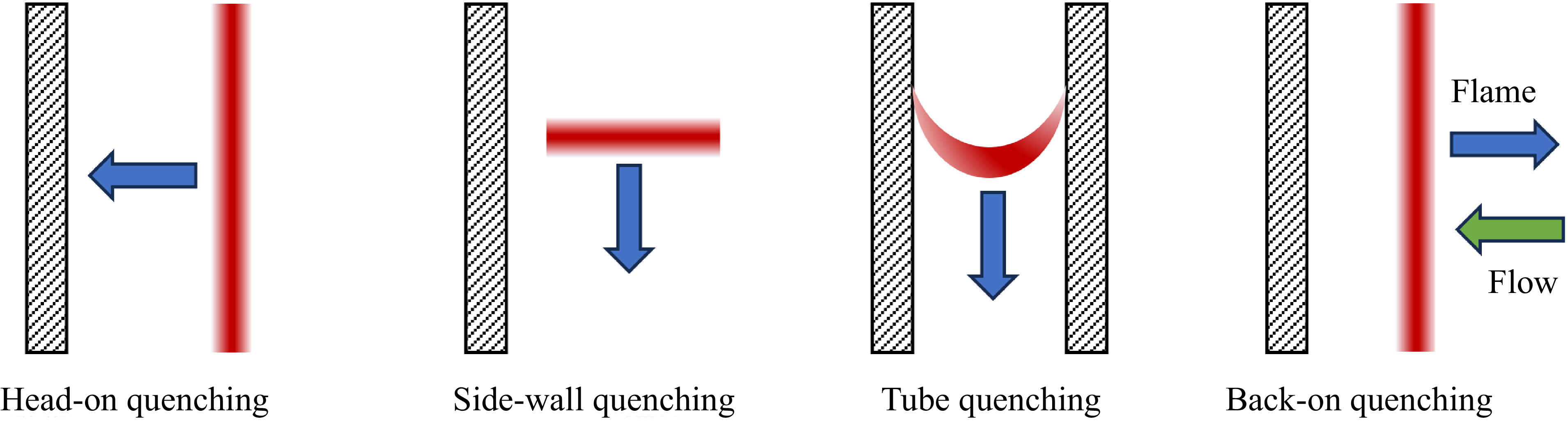


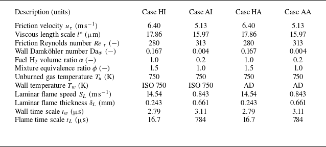


 Open access