

Introduction
Population monitoring of threatened species is necessary to verify recovery status, and allows managers to document population growth and detect population declines. To make effective decisions, managers must obtain information on a population's status within an appropriate time frame, and in small or Critically Endangered populations, early detection of population decline is critical to prevent extinction. Capture–recapture modelling is one of the most commonly used approaches for population monitoring (Otis et al., Reference Otis, Burnham, White and Anderson1978; Pollock et al., Reference Pollock, Nichols, Brownie and Hines1990; Williams et al., Reference Williams, Nichols and Conroy2002). Traditional methods of physical capture inherently involve risk and the potential for injury or mortality for both animals and researchers. Non-invasive genetic sampling combined with capture–recapture methods (genetic capture–recapture) eliminates much of that risk, provides reliable population estimates, and can be more cost efficient compared to other methods such as radio-collaring and aerial telemetry (Solberg et al., Reference Solberg, Bellemain, Drageset, Taberlet and Swenson2006; DeBarba et al., Reference DeBarba, Waits, Genovesi, Randi, Chirichella and Cetto2010b).
Even with non-invasive approaches, obtaining adequate sample sizes and sufficient recapture rates can be difficult or costly with species that occur in low numbers or in low densities. Abundance estimates generated from small sample sizes are often biased and are subject to low precision (Robson & Regier, Reference Robson and Regier1964), and thus conducting sampling at a time and location that maximizes the probability of capture improves the chance of success. Accuracy and precision can be affected by multiple factors, including number of sampling sessions, sample size, and failure of poor-quality samples (Burnham, Reference Burnham1987; Lukacs & Burnham, Reference Lukacs and Burnham2005; Settlage et al., Reference Settlage, Van Manen, Clark and King2008; Laufenberg et al., Reference Laufenberg, Van Manen and Clark2013). By evaluating potential biases related to specific capture–recapture methods and implementing a case-specific study design, researchers are more likely to attain the desired level of accuracy and precision.
The Sonoran pronghorn Antilocapra americana sonoriensis, endemic to the Sonoran Desert of the USA and Mexico, is categorized as Least Concern on the IUCN Red List (IUCN SSC Antelope Specialist Group, 2016) but was listed as endangered in 1967 under the U.S. Endangered Species Act (USFWS, 2015), and the Mexican population is listed on CITES Appendix 1. Abundance is currently estimated on a biennial basis using aerial counts corrected with sightability models (USFWS, 2015). Annual counts are not conducted because of the high cost. Aerial surveys indicate the US population increased from an estimated 21 (95% CI 18–33) individuals in 2002 to 202 (95% CI 171–334) in 2014 (USFWS, 2015). Estimated abundance from previous genetic capture–recapture research conducted on the portion of this population using developed water sites (an estimated 70% of the population; J.J. Hervert, Arizona Game & Fish Department, pers. comm.) was 121 (95% CI 112–132) in 2014 (Woodruff et al., Reference Woodruff, Lukacs, Christianson and Waits2016b). Although the genetic capture–recapture estimate is known to be biased low, as not all pronghorn use the drinkers (168 individuals were seen during the multi-day aerial survey; J.J. Hervert, pers. comm.), the results suggest a significant proportion of the population was sampled using these methods (Woodruff et al., Reference Woodruff, Lukacs, Christianson and Waits2016b). We also cannot exclude the possibility that the aerial survey is biased high, as the same individual could potentially be observed and counted more than once during the multi-day survey.
One concern with the current aerial survey method is the low power to detect small, but potentially significant, changes in abundance as a result of large confidence intervals, whereas this is not a problem with the narrow confidence intervals (and resulting high precision) from the genetic capture–recapture estimate. Additionally, reduced sampling effort and the use of a simpler method (i.e. single session as opposed to multi-session analysis) provides managers the option to save both time and money (i.e. fewer samples collected and analysed and no need to contract an outside entity to conduct the analysis).
In this study we used simulation modelling to evaluate various genetic capture–recapture sampling designs for monitoring Sonoran pronghorn abundance on the Cabeza Prieta National Wildlife Refuge and the adjoining Barry M. Goldwater Range. The overall goal was to determine the optimal sample size required to yield precise abundance estimates and to evaluate the reliability of single and multi-session abundance estimators. Using data simulated with varying sampling intensity, we evaluated the differences in abundance estimates and associated precision using closed capture models implemented in MARK (White & Burnham, Reference White and Burnham1999) and single-session capture–recapture models in capwire (Miller et al., Reference Miller, Joyce and Waits2005). We also performed a cost comparison between genetic capture–recapture methods compared to population estimation methods currently used for this species (i.e. aerial survey with sightability correction) focusing on the cost of obtaining comparable data from both of these methods.
Methods
This study included simulated data generated based on a previously analysed data set from a multi-session closed population faecal DNA study of Sonoran pronghorn conducted on the Cabeza Prieta National Wildlife Refuge and Barry M. Goldwater Range, in south-western Arizona, USA. Single-session methods were not used in the previous analysis. We used results of previously published data on deposition rates (Woodruff et al., Reference Woodruff, Johnson and Waits2015) and sex ratios (Woodruff et al., Reference Woodruff, Lukacs, Christianson and Waits2016b) to inform our simulation design. We provide relevant details of the previously collected data, but see Woodruff et al. (Reference Woodruff, Lukacs, Christianson and Waits2016b) for a complete description of the study. Within each of 2 years, 2013 and 2014, we collected pronghorn faecal samples at 11 drinkers (developed water sites) during 1–3 sampling sessions per drinker. We extracted and genotyped 494 and 692 faecal samples in 2013 and 2014, respectively, at 10 nuclear DNA microsatellite loci and one sex identification locus. We identified 91 and 100 unique individuals at drinkers in 2013 and 2014, respectively.
We developed full likelihood parameterization models (Otis et al., Reference Otis, Burnham, White and Anderson1978) in MARK (White & Burnham, Reference White and Burnham1999). Because capture/recapture probability varied by group (sex and age), abundance was estimated separately for adult males, adult females, and fawns. Sex was determined via genetic techniques, and we determined age using size and morphology of faecal pellets (Woodruff et al., Reference Woodruff, Johnson and Waits2016a). Population estimates were summed, and we calculated 95% confidence intervals using the Delta method (Seber, Reference Seber1982). To evaluate relative support for each model, we used Akaike's information criterion corrected for small sample size (AICc). The top abundance estimation model included equal detection and redetection probabilities, both varying by time and group (i.e. males, females, fawns; Woodruff et al., Reference Woodruff, Lukacs, Christianson and Waits2016b). Abundance was estimated to be 116 (95% CI 101–132) at drinkers in 2013 and 121 (95% CI 112–132) in 2014 (Woodruff et al., Reference Woodruff, Lukacs, Christianson and Waits2016b).
Simulations
To estimate the optimal number of consensus genotypes needed for precise abundance estimates (CV ≤ 10–20%; Pollock et al., Reference Pollock, Nichols, Brownie and Hines1990), we simulated closed populations emulating our non-invasive genetic sampling framework. Because we assumed all samples achieved a consensus genotype in simulations, number of samples collected refers to number of successful genotypes obtained (hereafter, samples). Approximately 75% of field-collected faecal samples achieved consensus genotypes (Woodruff et al., Reference Woodruff, Lukacs, Christianson and Waits2016b) and thus the actual number of samples collected would be c. 33% higher (e.g. for 300 consensus genotypes, you collect 400 samples). We used true population sizes of 100, 150, 200, 250 and 300 with a male : female ratio of 0.66 : 1. This ratio reflects sex ratios in our study area as estimated by managers during aerial counts (J.J. Hervert, pers. comm.).
We applied a simulation method for the single session (capwire) and multi-session (MARK) estimators separately because the sampling designs are substantially different (see Supplementary Material 1 for R code). We sought to simulate collecting the same number of scats for each design. Therefore, the target number of scats was collected in a single session in the capwire simulation but spread over multiple sessions in the MARK simulation. This represents the way sampling would be designed in a field study for each of these methods. For each simulated sampling session we looped through the animal population and assigned scat deposition. Then, we simulated detection of the deposited scats. Finally, we estimated population size using R packages for each method (capwire: Pennell et al., Reference Pennell, Stansbury, Waits and Miller2013; RMark: Laake, Reference Laake2013).
Individuals with higher deposition rates were set to have a higher probability of being sampled. Previous research indicated deposition rates averaged one pellet pile per pronghorn per day (Woodruff et al., Reference Woodruff, Johnson and Waits2015) and an approximately equal ratio of males and females visiting drinkers (as seen on remote cameras; S. Doerries, University of Arizona, pers. comm.). However, our results (Woodruff et al., Reference Woodruff, Lukacs, Christianson and Waits2016b) indicated 2.5–3 times more male than female samples at the drinkers and a male : female sex ratio of c. 1.5 : 1. Given this information, we assumed males have higher deposition rates than females. Thus for 1–3 sessions we chose to simulate mean deposition over a 7-day period, with males having twice the mean deposition rate of females. We simulated sampling every 7 days as, per current agency procedures, each drinker is visited c. every 7 days for restocking of supplemental feed. Per session, we randomly selected 50–600 samples with replacement, allowing individuals to be sampled more than once in a sampling session (i.e. 0–x times, where x is the total number of depositions by an individual; Supplementary Table 1). With a range of 50–750 samples collected in each session for any particular population size, the resulting consensus genotyping rate was 0.33–3.33 times per individual in a session (i.e. 50–500 samples per session for 150 individuals). Not all ratios (e.g. 0.33, 1.5 or 3.33 times) or number of sampling sessions were employed for every sampling design (Supplementary Table 1). All simulations were conducted in R 3.3.0 (R Development Core Team, 2013).
Abundance estimation and comparison of methods
To compare sampling design and estimators, we estimated abundance using both multi- and single-session modelling approaches. In multi-session models, populations are sampled during > 1 sessions at distinct time points or within discrete sampling sessions (Chao, Reference Chao2001). Although there may be multiple captures of the same individual within a sampling session, only a single capture per individual per sampling session is counted, resulting in binary data (1 = captured, 0 = not captured). In contrast, single session sampling, such as in capwire, uses the total number of captures (count data) for each individual and allows capture of an individual multiple times within sessions (Miller et al., Reference Miller, Joyce and Waits2005). The individual identification represents the animal's mark, yet all captures in all sessions are included, creating a capture distribution.
For multi-session models we used the top model (described above) implemented in RMark, to build the multi-session model. For every true abundance in each sampling design we simulated 100 datasets for estimating abundance and 95% confidence intervals using MARK and capwire. Simulations included one session in capwire, and two and three sessions in MARK.
A likelihood-ratio test in capwire chooses between the two available models: the even capturability model (ECM), which assumes individuals have an equal chance of being captured, and the two innate-rates model (TIRM), which models two mixtures of capturability (a lower and a higher rate) and is comparable to heterogeneity models. In capwire the likelihood ratio indicated the TIRM model was the appropriate model in all cases, and thus we did not estimate sex and age classes separately, as capwire inherently accounts for variation in capture probability when using the TIRM model (Miller et al., Reference Miller, Joyce and Waits2005).
Abundance estimates and confidence intervals were averaged over the 100 simulations. We evaluated the performance of each sampling design and estimator by comparing the simulated abundance estimates to the true population size (per cent bias), the coefficient of variation (CV), and the relative mean squared error (RMSE). We calculated the CV as the ratio standard error : estimate expressed as a per cent (Buckland et al., Reference Buckland, Anderson, Burnham, Laake, Borchers and Thomas2001) to evaluate the precision of each sampling design and estimator. The CV is commonly used to describe the precision of an abundance estimate. As a general rule, CV < 10% is ideal but < 20% indicates a precise estimate (White et al., Reference White, Anderson, Burnham and Otis1982; Pollock et al., Reference Pollock, Nichols, Brownie and Hines1990). Thus, determining an acceptable level of precision is dependent on the question being asked (e.g. What is the harvest limit? Or how much is this population growing or shrinking?; Mowat, Reference Mowat2005). RMSE incorporates accuracy (bias) and precision (variance), and low values indicate better performance and a good balance between bias and precision. Additionally, we examined the 95% confidence interval (CI) coverage probability, the proportion of times (out of 100 in this case) the true value was contained within the interval.
Cost comparison
We recognize that a direct comparison of costs associated with different methods of sampling is difficult given the different tasks and information acquired with each method; however, we chose to evaluate the cost of obtaining an abundance estimate using aerial methods versus genetic capture–recapture methods. The cost of aerial flights changes little, if at all, with an increase in population size. The cost of genetic capture–recapture methods, however, generally increases with an increase in population size and the need to collect and analyse more samples. Using our simulation results, we determined what level of sampling effort (i.e. sample size and number of sessions) would produce a CV equivalent to that of the aerial methods (c. 21%) at true abundance equal to the 2014 aerial survey estimate (202, 95% CI 171–334). We also determined the cost for genetic capture–recapture to obtain a more precise CV of at least 10% with 200 individuals.
For genetic capture–recapture, costs included supplies for sample collection, DNA extraction and analysis, and associated labour for field and laboratory work (i.e. time spent collecting samples, recording them in a database, extracting DNA, generating consensus genotypes and a capture history; Supplementary Table 2). The time does not include conducting analysis for abundance and/or survival estimates. This is difficult to estimate as it will vary based on experience and could be conducted by in-house personnel or by a contractor. We also did not include travel time to the drinkers because management personnel visit drinkers for other management tasks with the same frequency (c. every 7 days) as our genetic capture–recapture sampling design. Travelling to distant locations will obviously result in increased fuel and time costs and must be accounted for in the study design. Although the time required for sample collection will vary between studies, we estimated c. 27 hours annually (2 technicians at 13.5 hours each) for collection of 1,000 samples. As pay rates vary between field and laboratory personnel, labour costs were based on an average rate (USD 25.00/hour). For comparison, we divided the cost of the biennial flight into an annual cost. This cost includes flight time and pilot salary, but does not include the salaries of personnel conducting the counts or personnel performing analysis of sightability models.
Results
Simulations
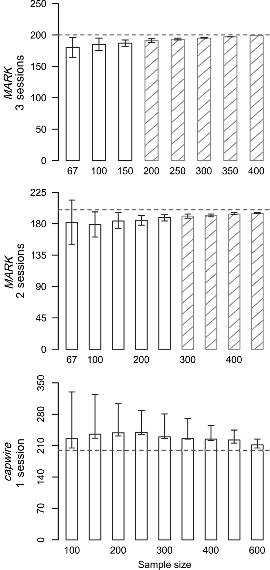
We ran 126 simulations (83 in MARK, 43 in capwire) varying sampling intensity and true abundance, with estimator performance dependent on sample size and true abundance (Fig. 1, Supplementary Table 1). As expected, increasing sample size (relative to number of sessions and number of individuals) generally led to less bias and lower RMSE values for both estimators. Abundance estimates were always positively biased in capwire (mean bias = 14.58%) and always negatively biased in MARK (mean bias = −4.88%). Bias ranged from overestimating by 64 individuals to underestimating by 25 individuals, and was larger with higher population sizes and with fewer samples per individual (Table 1). The CV was < 10% in 100% of MARK simulations and 84% of capwire simulations (Supplementary Table 1). Two capwire simulations had CV > 20%, both of which had relatively low sampling rates of ≤ 0.75 samples/individual/session.
Abundance estimates (y axis) from simulations for Sonoran pronghorn Antilocapra americana sonoriensis, with true abundance of 200 individuals in one session for single session models in capwire and two and three session closed capture (MARK) models. No shading indicates relative mean squared error (RMSE) > 0.5, and hatching represents RMSE ≤ 0.5. Trends were the same in all simulations but see Supplementary Table 1 for complete results.
A comparison of costs, and bias and precision (CV and RMSE), between aerial sighting and non-invasive genetic sampling capture–recapture methods.
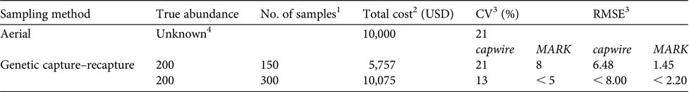
1 Number of consensus genotypes and represents 75% of the number of samples collected to account for failed samples because of DNA degradation.
2 Cost of aerial method includes cost of flight time and pilot but not associated salaries for personnel (USFWS, 2015). See Supplementary Table 2 for what is included in genetic capture–recapture cost.
3 CV for aerial methods is based on sightability. Capwire is single session and MARK is two sessions.
4 2014 population estimate from aerial surveys was 202, 95% CI 171–334.
The CI was 0–106% of the true abundance, and overall MARK had narrower confidence intervals than capwire. The CI in capwire was 0–0.73 probability coverage. The highest probability of coverage came from simulations with the lowest ratio of samples per individual (e.g. 0.5 samples/individual) and coverage probability decreased as the ratio increased (Fig. 1, Supplementary Table 1). Probability of CI coverage in MARK was ≤ 0.56. Capture probabilities in MARK were high (0.29–1.00) and mean capture probabilities for males were higher than those of females. High capture probabilities led to extremely precise estimates, which often missed the true abundance by 1 or 2 individuals (i.e. true abundance = 150, estimate = 149, CI 149–149). However, nearly all (99%, n = 82) MARK estimates were within 10% of the true abundance (e.g. 180 or 220 for true abundance of 200). On the contrary, a ratio of three samples per individual was required to achieve ≤ 10% bias in capwire.
Overall, RMSE decreased with increasing sample size (Fig. 1, Supplementary Table 1). When comparing total number of samples between the estimators (e.g. 200 total samples in one session for capwire or over two sessions in MARK), RMSE was consistently lower in MARK compared to capwire. Additionally, with larger population size, the gap was larger between RMSE values in MARK and capwire RMSE values with comparable sample sizes. For example, with a population of 300, there were 600 total samples in one session for capwire but spread over two sessions in MARK, and RMSE values indicated better overall performance with MARK (0.249) than capwire (5.31).
Cost comparison
The cost of the aerial survey is USD 10,000 annually (i.e. half of the cost of the biennial count; USFWS, 2015). To obtain a CV equal to the CV from the aerial estimate (21%), genetic capture–recapture simulations (population size = 200) indicated 0.75 samples/individual (confirmed consensus genotypes) were needed in just a single sampling session (capwire) at a cost of USD 5,757 (Table 1) with RMSE = 6.48. For the same cost, MARK (two sessions) substantially outperformed capwire, with CV = 8% and RMSE = 1.45. For the same cost as the aerial survey, estimates from genetic capture–recapture methods (MARK, two sessions: CV < 0.5; RMSE < 2.2) are markedly more robust. At this cost precision is also improved over aerial estimates with capwire (CV < 0.13) although RMSE is much higher (< 8.0) than when using MARK. Considering only the costs, aerial surveys become more cost effective at a population of c. 350 (cost per sample = USD 28.78, Supplementary Table 2; USD 10,000/28.78 = 347).
Discussion
Using an abundance estimator that provides the most accurate and precise estimate is particularly important when managing threatened species. A highly precise overestimate of the population would give the impression that the species is more abundant, and could result in the implementation of improper management actions (Noss et al., Reference Noss, Gardner, Maffei, Cuéllar, Montaño and Romero-Muñoz2012). Our study illustrates the need to use the appropriate sampling design and estimator in capture–recapture studies, and the inherent trade-off between the accuracy and precision of an abundance estimate and the effort and cost of monitoring. In our simulations the multi-session MARK model performed better than the single-session capwire estimator, indicating a clear optimal estimation method. As hypothesized, given the very high precision (CV c. 2%) in our previous genetic capture–recapture study (Woodruff et al., Reference Woodruff, Lukacs, Christianson and Waits2016b), substantial time and money can be saved by reducing sampling effort (e.g. fewer sessions, fewer samples) with little compromise in precision. Moreover, the genetic capture–recapture method has the potential to provide additional information on population genetic metrics and survival of different sex and age classes (Woodruff et al., Reference Woodruff, Lukacs, Christianson and Waits2016b).
Simulations can be used to design an efficient sampling scheme, but they are limited by the inability to exactly mimic field situations. To ensure our simulations mirrored field conditions as closely as possible we based simulated deposition and removal rates on previous work (Woodruff et al., Reference Woodruff, Johnson and Waits2015). True capture probabilities were very high (0.36–0.76; Woodruff et al., Reference Woodruff, Lukacs, Christianson and Waits2016b), and in simulations were 0.29–1.00. Consistent with Lukacs & Burnham (Reference Lukacs and Burnham2005), high capture probabilities (≥ 0.58) resulted in low bias (≤ 4%), although CI coverage was poor (mean = 0.18, range = 0.00–0.73). The simulations indicated highly precise estimates (i.e. low CV; mean CV capwire = 0.7; mean CV MARK = 0.2), yet this can be deceptive, as a low CV can still have high bias (Arnason et al., Reference Arnason, Schwartz and Gerrard1991; Supplementary Table 1). As expected, and consistent with other studies (Miller et al., Reference Miller, Joyce and Waits2005; Conn et al., Reference Conn, Arthur, Bailey and Singleton2006; Stenglein et al., Reference Stenglein, Waits, Ausband, Zager and Mack2010; Rees et al., Reference Rees, Goodenough, Hart and Stafford2014; Roy et al., Reference Roy, Vigilant, Gray, Wright, Kato and Kabano2014), increasing the sample size and number of sessions improved both the bias and precision of the estimates.
Other studies comparing MARK and capwire have produced conflicting results. Robinson et al. (Reference Robinson, Waits and Martin2009) and Harris et al. (Reference Harris, Winnie, Amish, Beja-Pereira, Godinho, Costa and Luikart2010) found lower and more precise capwire estimates compared to MARK. The opposite was true in this study and others (Gray et al., Reference Gray, Vidya, Maxwell, Bharti, Potdar, Channa and Sovanna2011, Reference Gray, Vidya, Potdar, Bharti and Sovanna2014; Lampa et al., Reference Lampa, Mihoub, Gruber, Klenke and Henle2015), with lower, more precise abundance estimates in MARK compared to capwire. An alternative method to consider is collecting samples during multiple sessions and collapsing them into a single session model (e.g. capwire). Although this is a less preferred method, it is useful when there are not enough recaptures for MARK to effectively estimate abundance (Robinson et al., Reference Robinson, Waits and Martin2009).
Because capwire is designed for use with small population size (< 100; Miller et al., Reference Miller, Joyce and Waits2005), it is not surprising that as true abundance increased, the performance of capwire weakened. Given the input for our simulations (mean male deposition rates twice that of females), using the TIRM in capwire makes intuitive sense, and was supported by likelihood ratio results. Nevertheless, 100% of capwire estimates were high. This is common for the TIRM model when capture probabilities are equal (Miller et al., Reference Miller, Joyce and Waits2005), but that was not the case in our dataset. In the presence of heterogeneity, models that assume equal capture probability (e.g. Lincoln-Peterson, ECM in capwire) have been shown to underestimate populations (Seber, Reference Seber1982; Miller et al., Reference Miller, Joyce and Waits2005; Petit & Valiere, Reference Petit and Valiere2006; Puechmaille & Petit, Reference Puechmaille and Petit2007). To evaluate bias under this model, we ran several simulations post factum using the even capturability model (data not shown). Although per cent CI coverage did improve in some cases, as expected, abundance was always underestimated with these models. When using empirical data (SPW, unpubl. data), we observed conditions in capwire when the lower CI was higher than the estimate, which is indicative of the model not capturing the distribution of the data sufficiently (M.W. Pennell, University of Idaho, pers. comm.).
Based on our previous research with a higher number of male compared to female samples (Woodruff et al., Reference Woodruff, Johnson and Waits2015, Reference Woodruff, Lukacs, Christianson and Waits2016b), remote camera data indicating no difference in use of drinkers by males and females, (S. Doerries, pers. comm.), and a 0.66 male : 1 female ratio reported by Arizona Game and Fish Department in aerial survey results, we assumed a higher deposition rate for males in our study design. However, we recognize there could be other explanations for the skewed sex ratio in our samples. There may be a behavioural difference in drinker visitation between males and females, especially females with fawns, which are seen less frequently on cameras at drinkers (D. Christianson, University of Arizona, pers. comm.) or a potential (undetected) bias in males visiting drinkers as a result of the skewed sex ratio (2 males : 1 female) of food and water conditioned captive-released pronghorn in this population (USFWS, 2015).
Another comparable method to consider for estimating abundance is spatial capture–recapture that incorporates the inherent individual spatial heterogeneity within the model (Royle et al., Reference Royle, Chandler, Sollman and Gardner2013). By design, spatial capture–recapture assumes recaptures of the same individual at multiple locations. In our study system, there was little movement between sites and most of our individuals (92%) were detected at a single location both within and across years. However, in other systems this could be a potentially useful and robust method for estimating abundance.
Cost comparison
Determining the appropriate monitoring method depends on the data needed for management (e.g. abundance, survival, genetic diversity), yet resources are often limited, and effective management should employ efficient monitoring methods to ensure the costs do not outweigh the benefits (Possingham et al., Reference Possingham, Lindenmayer and Norton1993). An often-voiced concern regarding genetic capture–recapture methods is the high cost. High costs can be associated with development of primers, and optimizing multiplexes (Schwartz & Monfort, Reference Schwartz, Monfort, Long, MacKay, Zielinski and Ray2008; Beja-Pereira et al., Reference Beja-Pereira, Oliveira, Alves, Schwartz and Luikart2009), travel to sampling sites (Harris et al., Reference Harris, Winnie, Amish, Beja-Pereira, Godinho, Costa and Luikart2010), collection method (e.g. scat detection dogs; Arandjelovic et al., Reference Arandjelovic, Bergl, Ikfuingei, Jameson, Parker and Vigilant2015), or increased use of personnel (Poole et al., Reference Poole, Reynolds, Mowat and Paetkau2011). Although developing a new faecal DNA protocol can require a substantial initial investment, costs are reduced in subsequent years. Genetic capture–recapture costs increase with increasing population size whereas flight costs are constant. Therefore, genetic capture–recapture can be more cost efficient at small population sizes and flights become more cost efficient at large population sizes.
Several studies have found genetic capture–recapture methods were more cost-effective compared to other field-based methods (e.g. radio-collaring and aerial telemetry; Solberg et al., Reference Solberg, Bellemain, Drageset, Taberlet and Swenson2006; DeBarba et al., Reference DeBarba, Waits, Genovesi, Randi, Chirichella and Cetto2010b), yet a direct comparison of costs is difficult given the different tasks and information acquired with each method. In 2014 our results showed genetic capture–recapture methods were twice as expensive as aerial methods (USD 20,000 vs 10,000, SPW, unpubl. data). Importantly, for Sonoran pronghorn these monitoring methods are conducted at different times of year: genetic capture–recapture in May–June, when pronghorn are congregated at drinkers, and aerial in December, when pronghorn are spread out across their c. 7,000 km2 range. The wider geographical sampling of the aerial survey leads to a trade-off of lower precision in both detection probability and population estimation compared to genetic capture–recapture. Because of our targeted sampling design in genetic capture–recapture, any inference from our estimates applies largely to the individuals using drinkers. However, if the proportion of individuals not using the drinkers was known or could be reliably estimated, abundance estimates obtained using genetic capture–recapture could easily be extrapolated to the entire population. Analogous considerations are critical for other species monitored in a similar fashion, such as bighorn sheep Ovis canadensis (Schoenecker et al., Reference Schoenecker, Watry, Ellison, Schwartz and Luikart2015), or other species often congregated at watering holes or mineral licks (e.g. elephants Loxodonta spp., zebras Equus zebra).
Although our simulations indicate increase in precision with more samples, depending on desired accuracy, precision and budget, a wide range of sampling designs is feasible. Our results also indicate that at the current estimated population size (c. 200), a CV of c. 21% can be obtained using genetic capture–recapture methods for an annual cost saving of > USD 4,000 over aerial costs and would provide monitoring data annually rather than biennially. Other cost-saving measures for genetic capture–recapture include collecting and analysing only the freshest samples (Lucchini et al., Reference Lucchini, Fabbri, Marucco, Ricci, Boitani and Randi2002) or decreasing the sampling interval with multiple sampling sessions (Marucco et al., Reference Marucco, Pletscher, Boitani, Schwartz, Pilgrim and Lebreton2009; Woodruff et al., Reference Woodruff, Johnson and Waits2015) for higher success rates (i.e. fewer failed samples). Additionally, the use of a simpler method such as capwire that can be easily implemented with minimal quantitative skills and training, as opposed to MARK, which requires significant knowledge of the software and modelling skills to obtain a reliable estimate, would also result in cost savings.
Methods such as physical capture and aerial telemetry and surveys may be undesirable because of concerns for human safety, impacts on wildlife and other natural resources, and logistical complexity. Moreover, these methods lack the ability to provide genotypic information on genetic diversity, relatedness, and genetic structure, which can provide valuable information on risk of inbreeding depression, population connectivity, effective population size, and parentage. This type of genetic monitoring would incur additional analysis time and labour cost but, depending on the questions being asked, could be conducted annually (e.g. for parentage analysis; DeBarba et al., Reference DeBarba, Waits, Garton, Genovesi, Randi, Mustoni and Groffs2010a), but more typically only once per generation (see Schwartz et al., Reference Schwartz, Luikart and Waples2007 and Stetz et al., Reference Stetz, Kendall and Vojta2011 for recommendations on designing a genetic monitoring programme).
Nevertheless, although potentially more expensive, aerial surveys allow the results to be available more quickly compared to genetic analysis. However, in areas with dense canopy cover (e.g. tropical or temperate rainforests) where aerial surveys are ineffective, genetic capture–recapture methods may provide one of the only reliable methods for estimating population abundance (e.g. Brinkman et al., Reference Brinkman, Person, Chapin, Smith and Hundertmark2011). Researchers must be aware of potential challenges associated with genetic analysis (e.g. difficulty obtaining permits to export samples, low success rates in some climates) or a lag time between data collection and results (i.e. shipping samples if required, sample processing time in laboratory, time for capture–recapture analysis).
The results of genetic capture–recapture in our study system presents a challenge for researchers given the very high capture probabilities that lead to results indicating high levels of precision, yet the estimates still exhibit bias. As far as we are aware our capture probabilities (0.42–0.83; Woodruff et al., Reference Woodruff, Lukacs, Christianson and Waits2016b) are up to twice as high as other published capture probabilities for ungulates (0.38 ± SE 0.047; Poole et al., Reference Poole, Reynolds, Mowat and Paetkau2011) and some of the highest reported in any capture–recapture study. Our results also highlight the importance of comparing estimator performance and cost prior to designing and implementing capture–recapture studies.
Management recommendations
Our research provides useful guidelines for designing a practical and cost-effective genetic capture–recapture monitoring strategy to obtain acceptable levels of accuracy and precision. This method can easily be adapted for use in areas where animals congregate, such as wintering areas, roosting sites, or along migration routes. Additionally, this method could be integrated with an occupancy approach to inexpensively document population expansion to new geographical areas. However, researchers should be aware that capture probabilities are rarely this high. In other systems, substantially more effort would probably be needed to obtain this level of precision. If there is high cost associated with more sampling sessions (i.e. an increased number of visits to sampling locations is more costly), it is feasible to collect more samples in fewer sessions. Although this would probably result in a biased, less precise estimate, managers may deem this trade-off of cost and level of accuracy and precision acceptable.
Acknowledgements
We thank Arizona Game and Fish Department, Cabeza Prieta National Wildlife Refuge and University of Arizona personnel for assistance with sample collection, J. Atkinson and J.J. Hervert for provision of time and expertise, M. Smith and K. Cobb for fieldwork, the Waits lab and D. Christianson for comments on the text, and J. Adams for laboratory assistance. This material is based upon work supported by, or in part by, the U.S. Army Research Laboratory and the U.S. Army Research Office under contract/grant number RC-201205.
Author contributions
Study design: SW, PL and LW. Fieldwork and data collection: SW. Data analysis: SW, PL and LW. Writing: all authors.
Conflicts of interest
None.
Ethical standards
All samples were collected in accordance with methods approved by the University of Idaho Institutional Animal Care and Use Committee (permit no. 2013-79).


