





Introduction
Self-localization is an important element in modern railway operation. Since trains require long braking distances and often lack direct line-of-sight to other vehicles, precise and reliable positioning is essential for ensuring safe operation and maintaining efficient traffic flow. Due to their constrained movement, it typically involves track-relative localization, which identifies the specific track and the traveled distance along it.
To estimate traveled distance, odometry and wheel sensors are commonly used, measuring distance either directly or by integrating velocity over time [Reference Otegui, Bahillo, Lopetegi and Díez3, Reference Heirich, Siebler, Sand, Lehner and Crespillo4]. However, these methods are prone to sensor drift, where small errors accumulate over long distances or under low-traction conditions, leading to growing uncertainty. To mitigate this, modern systems typically rely on sensor fusion with additional positioning sources. A possible approach is including absolute positioning from Global Navigation Satellite Systems (GNSS) and acceleration data from inertial measurement units (IMUs) [Reference Heirich5]. Although this combination can reduce uncertainty in distance estimation and assist with track identification, its effectiveness is constrained by the availability of GNSS signals and the accuracy of IMU sensors. In prolonged GNSS-denied scenarios, such as extensive tunnel networks and deep underground lines, this approach is insufficient to ensure reliable train operation. An alternative positioning approach involves using position-dependent signatures distributed along the track, such as passive magnetic signatures [Reference Heirich, Siebler and Hedberg6]. However, these can be affected by train traffic on adjacent tracks, and the recorded signatures may vary between measurement runs [Reference Heirich and Siebler7]. Within the European Train Control System (ETCS), absolute position on the track can be determined using trackside balises, which encode location-specific information and are read during traversal. While highly accurate, this approach relies on track-bed infrastructure, which may be vulnerable to displacement or sabotage. Additionally, complex track layouts often necessitate a high density of balises, leading to high installation and maintenance costs. Consequently, reducing the number of required balises for reliable and safe operation is desirable. Distance-based localization can be enhanced by detecting landmarks such as infrastructure elements like switches, bridges, and overpasses, which have fixed positions within the track network. Recognition of these elements can provide reference points that, when compared with a known track layout, enable correction of odometry drift and support determining the route taken at diversion points, thereby reducing reliance on dedicated hardware such as balises. Optical sensors such as cameras have been used for switch detection and classification [Reference Jahan, Niemeijer, Kornfeld and Roth8], but their dependence on visibility and susceptibility to adverse weather limit their operational robustness. Ground-penetrating radar (GPR) offers a reliable alternative, operating independently of visibility and resistant to environmental factors such as precipitation or icing [Reference Ort, Gilitschenski and Rus12]. GPR has already been investigated as a localization sensor for rail [Reference Noll, Kohnert, Caldero and Seidel2] and non-rail vehicles [Reference Cornick, Koechling, Stanley and Zhang9–Reference Bi, Shen, Zhang, Huang, Xin and Jin11]. Its ability to capture rich surface and subsurface reflections makes it well-suited for extracting distinctive features of infrastructure elements.
In this work, GPR measurements from multiple trips across a regional railway network are analyzed to detect and classify infrastructure elements such as switches, bridges, and overpasses. Multi-channel GPR data are processed through a preprocessing pipeline and converted into spatial B-scans. Statistical and structural features are extracted using a sliding window approach, calibrated against reference measurements, and reduced to a set of three features per measurement channel. Distinctive feature profiles for infrastructure elements are identified, and reference patterns for switches are generated. Classification is performed in a streaming manner by correlating current feature windows with reference patterns and applying threshold-based metrics. A decision system integrates both approaches for element identification and switch type discrimination. Evaluation of multi-trip recordings demonstrates effective detection and reliable classification under real-world conditions.
An earlier version of this paper was presented at EuMW 2025 and was published in its Proceedings [Reference Noll, Kohnert and Caldero1].
Track network & infrastructure elements
For this investigation, seven independent evaluation trips, recorded over two consecutive days in August 2021 between Rothensee, Wolmirstedt, and Magdeburg, Germany, are evaluated. Together, these trips covered  $57.4\,$km and resulted in a mapped track network of $23.5\,$km. An additional reference trip, outside of this network, was recorded near Rothensee for calibration.
The network mainly consists of ballasted track superstructures, railway tracks laid on a bed of crushed stone, as well as several key infrastructure element types. It includes 27 switches, mechanical installations that enable trains to change tracks, 11 overpasses, which allow railway lines to cross above roads, and 5 bridges with prominent metal elements at the track surface, load-bearing structures that span physical barriers such as waterways or valleys. Two of the evaluated bridges are provisional metal constructions, temporarily installed to facilitate underpass construction at Wolmirstedt station. Additionally, the network includes three railroad crossings, each traversable in four ways, straight or with lane changes from either side. Since only a subset of these approaches is represented in the measurement data, key variations are missing, and these elements are therefore excluded from the evaluation due to incomplete coverage in the reference and evaluation datasets. Most elements were traversed multiple times at different speeds and directions, which increases the number of classification scenarios beyond the actual count of physical elements.
Measurement setup & initial signal processing
During the conducted trips, GPR measurements were collected using the multi-channel sensor array shown in Fig. 1.
Overview of the GPR sensor array (left) and corresponding platform view (right). Measurement channels  $p=\{1,\ldots,4\}$ span the track width. Only the front row of sensor is used for the evaluation.

Figure 1 Long description
The left image shows a Ground Penetrating Radar (GPR) sensor array mounted on the front of a train. The array consists of multiple red sensor units connected by cables and supported by a metal frame. The train is positioned on tracks in an outdoor setting. The right image is a schematic illustrating the arrangement of the GPR sensors. It depicts four measurement channels labeled p equals 1, p equals 2, p equals 3 and p equals 4, each associated with a GPR unit. The train is shown in relation to the track, with an arrow indicating the travel direction. The schematic provides a top-down view of the sensor placement across the track width.
The setup comprises four GSSI 50400S modules with a center frequency of  $400\,$MHz, providing $P=4$ measurement channels $p=\{1,\ldots,P\}$ that span the entire track width. These modules are operated monostatically via a GSSI SIR 30 controller unit, featuring a $32\,$bit resolution and a pulse repetition frequency (PRF) of $1.2\,$kHz. Additionally, a DRS05 Doppler radar from Deuta is employed as a velocity reference.
Sequentially, each module transmits a  $2.5\,$ns pulse, which is partially reflected at boundaries between surface and subsurface materials with differing dielectrical properties. After transmitting its pulse, the module records the resulting superimposed echoes within a $60\,$ns time window, sampled at $265$ discrete and evenly spaced intervals. Each recorded sequence constitutes an A-scan, where the time axis is referred to as the fast-time dimension. Since the pulse propagation velocity is expected to vary between materials, a direct assignment between fast-time and penetration depth is omitted. Instead, the term “depth” is used solely in a descriptive sense.
To enhance signal quality and interpretability, an initial signal processing chain is applied to the data stream of each channel. First, constant signal components are removed using a background subtraction, where each A-scan is subtracted from its predecessor. Next, depth-related attenuation is mitigated by applying a time-varying gain that exponentially amplifies the A-scan’s amplitude along its fast-time dimension. Noise is then reduced using a matched filter, with a second-order Gaussian wavelet employed as an approximation for the transmitted pulse. Subsequently, the signal envelope of the A-scan is estimated via Hilbert transformation. The A-scans are then downsampled by a factor of two to reduce the amount of data. After A-scan processing, scans from each channel are arranged in sequence and linked to the vehicle’s traveled distance by integrating the reference velocity. The distance is discretized into range bins of  $5\,$cm, and all A-scans within a single bin are averaged, resulting in a spatial B-scan for every channel. Figure 2 shows an example B-scan from the fourth channel $p=4$, illustrating the transition from an overpass to a switch. To normalize B-scan values, percentile-based scaling is applied. Scaling and offset parameters are derived from the reference measurement for each channel, mapping values between its 50th and 98th percentiles to the normalized range [0,1]. These parameters are then applied to the measurements of the evaluation trips, and any outliers are clipped to maintain consistency. Finally, the fast-time range is limited to a depth region of $3.5$– $15\,$ns, where infrastructure-related signal patterns are prominent.
Spatial B-scan (channel  $p=4$) at an overpass-to-switch transition. The highlighted red region marks the current measurement window and travel direction. The middle plot shows corresponding feature profiles, with current values emphasized. The lower plot presents the feature strip (gray box) for the window, illustrating its integration into a multi-channel feature map.

Figure 2 Long description
The top plot displays a spatial B-scan with fast time on the y-axis ranging from 5 to 15 nanoseconds and distance on the x-axis from 190 to 215 meters. The highlighted red region indicates the current measurement window and travel direction. The middle plot shows feature profiles with the y-axis labeled 'Feature' and the x-axis labeled 'Distance (m)'. Three curves are visible: ENR (red), DEP (green) and SKW (blue), each showing different trends across the distance range. The lower plot presents a feature strip with 'Channel p' on the y-axis and 'Distance (m)' on the x-axis, illustrating integration into a multi-channel feature map. The legend at the top categorizes sections as Steel Bridge, Regular Track, Switch and Overpass.
The center frequency of  $400\,$MHz was dictated by the measurement setup, which was also used to provide data for the investigation of subsurface features [Reference Noll, Kohnert, Caldero and Seidel2]. Since only near-subsurface features are being utilized here, the center frequency could be increased, thereby improving the resolution and potentially strengthening the robustness of the approach.
Feature selection & calibration
Features for infrastructure detection and classification are extracted from the spatial B-scans by a sliding window approach. This is performed independently for each channel and is illustrated for  $p=4$ in Fig. 2. A $1\,$m window, highlighted within a red box, moves along the spatial B-scan in the travel direction. It advances in $0.5\,$m steps, creating a $50\%$ overlap between consecutive windows. Each window $\boldsymbol{X} \in \mathbb{R}^{M \times N}$ is represented as $30\times 20$ matrix, where $M=30$ corresponds to the fast-time dimension and $N=20$ to the spatial dimension. From each matrix, a set of feature values is computed, encoding its signal characteristics. As the window shifts along the B-scan, these values are collected sequentially, forming along-track feature profiles for each channel. This is illustrated in the middle plot of Fig. 2, which shows the corresponding feature profiles extracted from the upper B-scan, while the highlighted points indicate the feature values extracted from the current window.
Because extraction relies on small sections of typically similar B-scans, commonly used descriptors for 2D matrices are often highly correlated. To reduce redundancy, a compact set of three representative features is selected. Encoding these features as a three-channel color representation additionally provides intuitive visualization for qualitative analysis. The selected features can be described by:
 \begin{equation}
\text{Energy (ENR):} \quad \displaystyle\sum_{m,n}x_{m,n}^2
\end{equation}
\begin{equation}
\text{Energy (ENR):} \quad \displaystyle\sum_{m,n}x_{m,n}^2
\end{equation} \begin{equation}
\text{Depth (DEP):} \quad \displaystyle\left[ 1,2,\dots,M\right]\frac{\tilde{\boldsymbol{x}}^3}{\sum_m{\tilde{x}_m^3}}
\end{equation}
\begin{equation}
\text{Depth (DEP):} \quad \displaystyle\left[ 1,2,\dots,M\right]\frac{\tilde{\boldsymbol{x}}^3}{\sum_m{\tilde{x}_m^3}}
\end{equation} \begin{equation}
\text{Skewness (SKW):} \quad \displaystyle\frac{\sum_{m,n} (x_{m,n} - \mu)^3}{(MN)\,\sigma^3}
\end{equation}
\begin{equation}
\text{Skewness (SKW):} \quad \displaystyle\frac{\sum_{m,n} (x_{m,n} - \mu)^3}{(MN)\,\sigma^3}
\end{equation} where,  $m \in {1, \dots, M}$ and $n \in {1, \dots, N}$ denote the fast-time and distance indices, respectively. The scalar value at position $(m,n)$ is denoted by $x_{m,n}$. The median A-scan of $\boldsymbol{X}$ is represented as $\tilde{\boldsymbol{x}} = (\tilde{x}_1, \dots, \tilde{x}_M) \in \mathbb{R}^M$. The parameters $\mu$ and $\sigma$ correspond to the mean and standard deviation of all entries in $\boldsymbol{X}$.
To ensure comparability between different features and channels, as well as to improve visualization, percentile-based normalization is applied. In this approach, values within the selected percentile range are mapped linearly to the interval  $[0,1]$. However, values outside this range may exceed the interval. The features energy ( $\mathrm{ENR}$) and depth ( $\mathrm{DEP}$) have approximately normal, and therefore symmetric, value distributions. Accordingly, a symmetric interval between the $0.1$st and $99.9$th percentiles is selected, effectively capturing the central data region and minimizing the influence of rare extremes. The skewness feature (SKW) exhibits a skewed distribution and is normalized using an asymmetric percentile window. The lower bound is set to the $0.1$st percentile of the longer tail, and the upper bound to the $90$th percentile of the shorter side. This choice expands coverage where variation is greatest while compressing the opposite side, ensuring the scaling emphasizes the most informative range. All percentile thresholds, scaling factors, and offsets for both normalization methods are calibrated using data from the reference trip and remain fixed for the evaluation trips.
For visual interpretation, each measurement channel  $p = \{1, \ldots, P\}$ is rendered as a colored strip, with each feature assigned to one color component. These strips are combined into a comprehensive feature map, as illustrated in the bottom plot of Fig. 2, where the color strip corresponding to the fourth channel $p=4$ is highlighted within a gray box.
Feature properties and switch sample pattern generation
The extracted features can now be analyzed within the track network, and general classification approaches for different infrastructure types derived. As an illustration, this is demonstrated for an example track section shown in Fig. 3, where track type and traversed infrastructure elements are indicated above the feature map.
Feature map (top) with various infrastructure elements highlighted. Below, the corresponding features for the measurement channels  $p=\{1,\ldots,P\}$ are shown in descending order: energy (ENR), depth (DEP), and skewness (SKW).

Figure 3 Long description
The top section displays a feature map with infrastructure elements highlighted: bridge, regular track, switch and overpass. Below are three graphs labeled ENR, DEP and SKW, representing energy, depth and skewness respectively. The x-axis for all graphs is labeled 'Distance' in meters, ranging from 0 to 400. The y-axis for ENR and DEP ranges from 0 to 1, while SKW ranges from 0 to 2. Each graph includes four curves labeled p equals 1, p equals 2, p equals 3 and p equals 4, distinguished by different colors. The curves show variations in measurements across the distance, with notable peaks and troughs at various points. The feature map and graphs together illustrate the relationship between track types and measurement channels over the specified distance.
Across regular track sections, feature patterns are generally consistent. However, the inner channels show slightly more variability, likely caused by the greater presence of mixed ballast material in the center of the track. In contrast, the outer channels remain more stable, which is probably due to the uniform reflection from the rails and fastening systems. Infrastructural elements such as bridges, underpasses, and switches introduce recognizable patterns in the feature map, often marked by unique coloration. In the case of elements like bridges and overpasses, these are very consistent and independent of travel direction. Furthermore, overpasses produce high SKW values beyond the normalized range, making them easily distinguishable. This consistent behavior enables a rule-based classification approach using predefined thresholds. However, variations in feature amplitude within the same element type can complicate threshold-based classification and need to be handled during the classification step.
Railroad switches are more complex, as illustrated in Fig. 4. On the left side are movable switch rails that determine the selected route. Due to the additional movable parts and more intricate fastening systems, switches comprise a larger amount of metal structures, which increases surface reflections leading to high ENR values (red). This region is referred to in this investigation as the switch center. After the switch center, the train passes one of the inner lead rails. These rails create consistently strong reflections in the upper part of the A-scans. During preprocessing, constant signal components are removed, which suppresses these reflections. As a result, the DEP feature (green) shows high values in the thrid channel p = 3 between  $5$–
$5$– $20\,$m and later in the second channel p = 2 between $23$–
$23$– $28\,$m. These traces are then followed by strong reflections from the guard rail. Similar to the lead rail, these reflections also correspond to high DEP values in the inner channel because the same preprocessing step affects them. However, guard rails are not always present, as they may be omitted in some configurations.
Overview of a representative railway switch. Left: schematic switch layout (top) and the corresponding reference pattern (bottom). The pattern segment used for switch matching is highlighted in red. Right: photograph of a switch in the field.

Figure 4 Long description
The left side shows a schematic of a railway switch layout with labeled sections: Switch Start, Switch Center, Transition Area, Lead Rail and Guard Rail. The diagram includes a color-coded channel representation with Channel p labeled from 1 to 4 and Distance in meters from 0 to 35. The right side displays a photograph of a railway switch in the field, showing the tracks and surrounding area.
Feature patterns at switches are influenced by both the traversal direction and the selected route, as shown in Fig. 5. For detailed analysis, switches are grouped into four types: Incoming-Left (IL), Incoming-Right (IR), Outgoing-Left (OL), and Outgoing-Right (OR). Patterns associated with different switch types exhibit a high degree of symmetry. Left and right variants can be aligned by mirroring around the vertical midpoint of the pattern, while incoming and outgoing variants can be aligned by mirroring around the horizontal midpoint. Due to this symmetry, the switch type can be identified by estimating the orientation of the observed pattern. Therefore, instead of using separate reference patterns for each switch type, a single reference pattern can be applied by adjusting for the corresponding orientation.
Overview of different switch scenarios with the corresponding patterns within the feature map.

Figure 5 Long description
The image consists of four diagrams illustrating different switch scenarios on railway tracks. Each diagram includes a labeled switch type and a feature map pattern. The top left diagram is labeled 'Incoming-Left (IL)' and shows a curved track with an arrow indicating the direction of incoming movement to the left. The top right diagram is labeled 'Outgoing-Left (OL)' and depicts a curved track with an arrow indicating outgoing movement to the left. The bottom left diagram is labeled 'Incoming-Right (IR)' and shows a curved track with an arrow indicating incoming movement to the right. The bottom right diagram is labeled 'Outgoing-Right (OR)' and depicts a curved track with an arrow indicating outgoing movement to the right. Each diagram features a green rectangle highlighting the switch area and a colorful feature map below the tracks, illustrating the pattern associated with each switch type.
For this reference pattern, 16 switch-related patterns from the reference trip are manually selected, then mirrored to ensure a consistent orientation. Each pattern is then resampled to a common length of  $35\,$m, which corresponds to the average and rounded length of the extracted switch patterns, and aligned using an iterative Dynamic Time Warping (DTW) process. This alignment reduces shape differences before averaging and normalizing the profiles. The resulting reference pattern, shown in the bottom plot of Fig. 4, forms the basis for the comparison pattern used in switch orientation classification. Only the highlighted $20\,$m transition segment is used, which improves classification performance despite variations in switch length or missing guardrails. Since regular track sections exhibit consistently high SKW (blue) values, the switch comparison pattern shows a pronounced deviation from regular track on one side, creating strong left-right asymmetry. This asymmetry can be exploited for orientation detection, as it can provide a clear directional cue during classification.
Classification approach
The encountered infrastructure elements can vary in length and spatial layout, which makes their boundaries unknown during processing. To handle this uncertainty, the proposed method, illustrated in Fig. 6, employs a streaming architecture that processes data sequentially without requiring prior segmentation. The system operates on a continuously updated  $20\,$m feature window $\boldsymbol{F}$ (green box). With a spatial resolution of $50\,$cm, each update replaces the last column of feature values with a new one. For offline processing, this corresponds to a sliding window operation similar to feature extraction. Detection and classification are realized through a state-machine decision system that integrates evaluation scores from two branches: one estimates switch orientation via correlation, while the other applies rule-based classification using predefined thresholds to identify infrastructure elements.
Overview of the streaming classification data pipeline. After spatial B-scan generation, channel features are extracted from  $1\,$m wide measurement windows $\boldsymbol{X}$ (red box). These are aggregated into the current $20\,$m feature window $\boldsymbol{F}$ (green box), then processed in parallel: feature-based thresholds for infrastructure detection (right) and correlation-based classification for switches (left). The resulting scores feed into a classification state machine.

Figure 6 Long description
The diagram illustrates a data pipeline for classification. It begins with preprocessing, labeled as spatial B-scans, followed by feature extraction to create a feature map. The process splits into two paths: A) Correlation-Based Switch Orientation Estimation and B) Feature-Based Infrastructure Evaluation. In section A, correlation is performed using C subscript IL, C subscript IR, C subscript OR and C subscript OL, followed by value adjustment and normalization. Section B involves normalization, transformation, thresholding and circular variance calculations. The final step is the classification process using a state machine, which integrates results from both paths.
Correlation-based switch orientation estimation
The correlation branch compares the current feature window  $\boldsymbol{F}$ with the generated switch comparison pattern. To handle different switch classes, rotated versions of this pattern, shown within the correlation box of Fig. 6, are correlated with the window, producing four correlation coefficients at each step: $c_{\text{IR}}, c_{\text{IL}}, c_{\text{OL}}, c_{\text{OR}}$. The progression of these values along the example section is illustrated in the top plot of Fig. 7. For reference, the correct orientations for the switches are: $180$– $260\,$m incoming-left (IL), $390$– $460\,$m outgoing-left (OL), $470$– $530\,$m incoming-right (IR), and $560$– $630\,$m outgoing-left (OL). The correlation values vary strongly between switches, and offsets in different track sections make direct interpretation unreliable. Moreover, incoming ( $c_{\text{IR}}, c_{\text{IL}}$) and outgoing ( $c_{\text{OL}}, c_{\text{OR}}$) coefficients often look similar due to the symmetry of the switch comparison pattern.
Correlation coefficients along an example track section. The top plot shows the original values for all four orientations  $c_{\text{IR}}, c_{\text{IL}}, c_{\text{OL}}, c_{\text{OR}}$. The middle plot illustrates the adjusted coefficients after subtracting half of their opposite orientation to increase differences, and the bottom plot shows the normalized values for improved interpretability.

Figure 7 Long description
The image contains three plots illustrating correlation scores across various track sections labeled as bridge, regular track, switch and overpass. The top plot displays channel p with a color-coded representation over a distance from 0 to 400 meters. The middle plot shows score c with four curves labeled OL, OR, IR and IL, each representing different orientations. The bottom plot presents score c hat, also with four curves labeled OL, OR, IR and IL. Each plot is segmented by colored sections corresponding to different track types, including yellow for bridge, blue for regular track, red for switch and light blue for overpass. The x-axis is labeled as distance in meters and the y-axis labels are channel p, score c and score c hat respectively.
Therefore, the coefficients are adjusted by subtracting half of their opposite orientation:
 \begin{equation}
\begin{bmatrix}
\hat{c}_{\text{IR}} \\
\hat{c}_{\text{IL}} \\
\hat{c}_{\text{OL}}\\
\hat{c}_{\text{OR}}
\end{bmatrix}
=
\begin{bmatrix}
1 & -0.5 & 0 & 0 \\
-0.5 & 1 & 0 & 0 \\
0 & 0 & 1 & -0.5 \\
0 & 0 & -0.5 & 1
\end{bmatrix}
\begin{bmatrix}
c_{\text{IR}} \\ c_{\text{IL}} \\ c_{\text{OL}} \\ c_{\text{OR}}
\end{bmatrix}.
\end{equation}
\begin{equation}
\begin{bmatrix}
\hat{c}_{\text{IR}} \\
\hat{c}_{\text{IL}} \\
\hat{c}_{\text{OL}}\\
\hat{c}_{\text{OR}}
\end{bmatrix}
=
\begin{bmatrix}
1 & -0.5 & 0 & 0 \\
-0.5 & 1 & 0 & 0 \\
0 & 0 & 1 & -0.5 \\
0 & 0 & -0.5 & 1
\end{bmatrix}
\begin{bmatrix}
c_{\text{IR}} \\ c_{\text{IL}} \\ c_{\text{OL}} \\ c_{\text{OR}}
\end{bmatrix}.
\end{equation} The adapted values  $\hat{\boldsymbol{c}}= [\hat{c}_{\text{IR}}, \hat{c}_{\text{IL}}, \hat{c}_{\text{OL}}, \hat{c}_{\text{OR}}]$ are shown in the third plot of Fig. 7. This step increases correlation differences at relevant distances ( $210\,$m: orange, $410\,$m: violet, $500\,$m: blue, $580\,$m: violet), while preventing overcompensation. For easier interpretation, these values are then normalized by centering them around their mean $\mu$ and multiplying them by their standard deviation $\sigma$:
 \begin{equation}
\tilde{\boldsymbol{c}} = \left( \hat{\boldsymbol{c}} - \mu \right) \cdot \sigma.
\end{equation}
\begin{equation}
\tilde{\boldsymbol{c}} = \left( \hat{\boldsymbol{c}} - \mu \right) \cdot \sigma.
\end{equation} As shown in the bottom plot of Fig. 7, this step amplifies distinctive variations near switches while suppressing similar values in regular track or overpass regions, facilitating orientation estimation. The  $\tilde{\boldsymbol{c}}$ values are then used as evaluation scores within the decision system.
Feature-based infrastructure evaluation
The second processing branch interprets the current feature window  $ \boldsymbol{F} \in \mathbb{R}^{P \times Q \times R} $ by analyzing the distribution and relationships of its feature values across channels $p=[1,\ldots,P]$, spatial positions $q=[1,\ldots,Q]$, and feature types $r=[1,\ldots,R]$. Here, $P = 4$ represents the number of channels, $Q = 40$ the spatial samples covering $20\,\mathrm{m}$ at $0.5\,\mathrm{m}$ resolution, and $R = 3$ the number of feature types. The feature values $f(p,q,r)\in\boldsymbol{F}$ are first normalized to yield their relative contribution at each position $(p, q)$:
 \begin{equation*}
|f(p,q,r)| = \frac{f(p,q,r)}{\sum_{r=1}^{R} f(p,q,r)}.
\end{equation*}
\begin{equation*}
|f(p,q,r)| = \frac{f(p,q,r)}{\sum_{r=1}^{R} f(p,q,r)}.
\end{equation*} This normalization emphasizes relationships between features rather than absolute values, which vary more within elements of the same type. Based on these normalized values, three binary evaluation scores are determined to indicate specific infrastructure types, while a contextual score represents overall feature variation. For the binary scores, the proportion of positions  $\pi$ where normalized values lie within a predefined range $[\lambda_r^{\min}, \lambda_r^{\max}]$ is calculated for each channel $p$ and feature type $r$:
$r$:
 \begin{equation*}
\pi_{p,r} = \frac{1}{Q}\sum_{q=1}^{Q} \mathbf{1}\!\left\{|f(p,q,r)|\in[\lambda_r^{\min},\lambda_r^{\max}]\right\}.
\end{equation*}
\begin{equation*}
\pi_{p,r} = \frac{1}{Q}\sum_{q=1}^{Q} \mathbf{1}\!\left\{|f(p,q,r)|\in[\lambda_r^{\min},\lambda_r^{\max}]\right\}.
\end{equation*}These proportions are compared against thresholds characteristic of specific infrastructure.. For bridges (bg) and overpasses (op), scores are given by:
 \begin{equation*}
s_{\mathrm{bg}}=\mathbf{1}\{\forall r:\overline{\pi}_{r}\ge\tau_{r,\text{bg}}\},\quad
s_{\mathrm{op}}=\mathbf{1}\{\forall r:\overline{\pi}_{r}\ge\tau_{r,\text{op}}\},
\end{equation*}
\begin{equation*}
s_{\mathrm{bg}}=\mathbf{1}\{\forall r:\overline{\pi}_{r}\ge\tau_{r,\text{bg}}\},\quad
s_{\mathrm{op}}=\mathbf{1}\{\forall r:\overline{\pi}_{r}\ge\tau_{r,\text{op}}\},
\end{equation*}where  $\overline{\pi}_{r}$ denotes the average of $\pi_{p,r}$ across all channels. For switches, a score $s_{\text{sc}}$ is determined to indicate the presence of switch centers. Due to the more complicated feature pattern at switches, this score must satisfy two conditions. The proportions $\pi$ for both outer channels $\mathcal{O} = \{1, 4\}$ must exceed their thresholds, and the highest proportion among all channels must belong to one of these outer channels:
 \begin{equation*}
s_{\mathrm{sc}} = \mathbf{1}\!\Big\{\forall r:\pi_{p,r}\ge\tau_{r,\text{sc}}\text{for }\mathcal{O}
\land \arg\max_{p}\pi_{p,r}\in\mathcal{O}\Big\},
\end{equation*}
\begin{equation*}
s_{\mathrm{sc}} = \mathbf{1}\!\Big\{\forall r:\pi_{p,r}\ge\tau_{r,\text{sc}}\text{for }\mathcal{O}
\land \arg\max_{p}\pi_{p,r}\in\mathcal{O}\Big\},
\end{equation*}where the argmax condition reduces misclassifications caused by guard rails.
The thresholds, derived from the calibration trip (Table 1), are set low to enable early detection during streaming. This allows the system to flag potential candidates promptly even when only partial patterns are present within the  $20\,$m window. In addition, a non-binary contextual score captures variations in feature relationships within the window. For this score, the feature window $\boldsymbol{F}$ is first smoothed along the dimensions $p, q$ for each feature type $r$ using a two-dimensional Gaussian kernel with a $5 \times 5$ window and standard deviation $\sigma = 2$. This smoothing reduces local noise within each feature type while preserving general changes. At each position $(p, q)$, the filtered feature values are then represented as a point in 3D Cartesian space ( $R = 3$) and mapped to spherical coordinates, from which the azimuth $\phi$ and inclination $\theta$ are derived. To quantify how feature relationships vary across the window, circular variance is used:
 \begin{equation*}
V_{\alpha} = 1 - \sqrt{\mathbb{E}[\cos\alpha]^2 + \mathbb{E}[\sin\alpha]^2},
\end{equation*}
\begin{equation*}
V_{\alpha} = 1 - \sqrt{\mathbb{E}[\cos\alpha]^2 + \mathbb{E}[\sin\alpha]^2},
\end{equation*}where  $\alpha$ denotes either $\phi$ or $\theta$, and $\mathbb{E}[\cdot]$ represents the mean over all positions $(p, q)$ within the window. Unlike linear variance, which only measures changes along a straight line, circular variance captures directional variability, showing how much the feature composition shifts in orientation. This provides an indicator for compositional changes within $\boldsymbol{F}$. Finally, the circular variance score $s_{\mathrm{cv}} \in [0, 1]$ is defined as the maximum of both variances:
 \begin{equation*}
s_{\mathrm{cv}} = \max(V_\phi,\, V_\theta).
\end{equation*}
\begin{equation*}
s_{\mathrm{cv}} = \max(V_\phi,\, V_\theta).
\end{equation*}Example configuration for percentage-based thresholds and feature ranges

Table 1 Long description
The table presents configuration data for percentage-based thresholds and feature ranges across three classes: $e_{\text{bg}}$, $e_{\text{op}}$, and $e_{\text{sc}}$. Each class is evaluated based on three features: ENR, DEP, and SKW. For $e_{\text{bg}}$, feature ENR has a range of 0.30 to 0.6, while for $e_{\text{op}}$, it is significantly narrower at 0.0 to 0.05. The SKW feature for $e_{\text{op}}$ shows a higher range of 0.7 to 0.85 compared to $e_{\text{bg}}$ and $e_{\text{sc}}$. All thresholds are consistent at 0.1, except for ENR in $e_{\text{sc}}$, which is 0.2. This data suggests variability in feature ranges across different classes, with consistent threshold values.
Values near  $0$ indicate consistent composition typical of homogeneous structures like bridges, overpasses, or ballast. Higher values reflect variability, common at switches, irregular sections, or transitions between elements, thus providing valuable context for classification.
Classification process
The classification process, illustrated in the bottom plot of Fig. 8, combines both branches using a state-machine decision system. This system assesses the binary evaluation scores, correlation-derived values, and contextual score to determine the most likely infrastructure for each feature window  $\boldsymbol{F}$. For bridges or overpasses, the classification is primarily based on the corresponding binary scores. To improve reliability and prevent false positives, a plausibility check is performed using the circular variance score. Upon the detection of a switch center, the classification process is dominated by the correlation scores. These scores are compared to determine the type of switch and to identify boundaries between adjacent switch centers (as shown between $250$– $300\,$m in Fig. 8). Once the end of a switch center or a boundary between centers is reached, the switch orientation is estimated using the observed correlation patterns. In cases where correlation differences are minimal (e.g., at $230$– $260\,$m), contextual information from the circular variance score becomes more dominant. By examining the length of feature variations before a switch center appears, the orientation is first estimated as incoming or outgoing and then refined to the most plausible left or right configuration.
Example feature map (top). The corresponding evaluation scores for bridges  $s_\text{bg}$, overpasses $s_\text{op}$, switch centers $s_\text{sc}$, and circular variance $s_\text{cv}$ are shown below, followed by correlation-based scores. At the bottom, the classification signals generated by the decision system are displayed.

Figure 8 Long description
The image consists of four distinct plots arranged vertically. The top plot displays a feature map with color-coded sections labeled as bridge, regular track, switch and overpass. The second plot shows binary scores with a line graph, where the x-axis is labeled 'Distance' in meters and the y-axis is labeled 'Binary Scores' with values ranging from 0 to 1. The third plot presents compact correlation scores with multiple line graphs, where the x-axis is labeled 'Distance' in meters and the y-axis is labeled 'Compared Correlation Correlation' with values ranging from -0.2 to 0.2. The fourth plot illustrates decision outputs with bars, where the x-axis is labeled 'Distance' in meters and the y-axis is labeled 'Element Detection' with values ranging from 0 to 1. Each plot is marked with specific sections corresponding to different infrastructure types and legends are present to indicate various elements within the graphs. Plot 2 and plot 4 also have a left y-axis.
Results
The proposed detection and classification approach was assessed on the evaluation trips. Raw GPR signals were processed sequentially through the complete pipeline: GPR A-scan processing, spatial B-scan generation, feature extraction, and final classification. To emulate real-world operation under constrained resources, evaluation was conducted in a streaming manner using a ring-buffer architecture.
Results are summarized in Fig. 9. Infrastructure detection and classification demonstrate high performance ( $\geq98\%$), with only one switch center (SC) undetected and no false positives. However, the number of measured bridges (5) is very low, which limits the statistical strength of conclusions regarding detection performance. Orientation classification also shows high reliability: incoming left (IL) and incoming right (IR) switches achieve $92\%$ and $82\%$, while outgoing left (OL) and outgoing right (OR) reach $94\%$ and $100\%$. Misclassifications occur only at the same set of closely spaced switches, which were recorded multiple times within the evaluation trips. In these cases, interference between adjacent patterns within the feature window reduces correlation distinctiveness. Moreover, physical interconnections between switches slightly modify feature patterns. Since these cases were absent in the reference trip, the reference signatures do not include them, which further reduces separability and increases wrong classifications.
Confusion matrix for infrastructure and orientation classification results on the measurement campaign. Rows denote predicted labels and columns denote ground truth.

Figure 9 Long description
The confusion matrix displays infrastructure classification results with predicted classes on the left and actual classes at the bottom. The matrix includes categories such as overpass, steel bridge, switch, incoming right, outgoing left, incoming left, outgoing right and no detection. Each cell shows the number and percentage of instances classified into each category. For example, 30 instances of overpass were correctly predicted, achieving 100 percent accuracy. Steel bridge has 8 correct predictions with 100 percent accuracy. Switch has 62 correct predictions with 98 percent accuracy. Incoming right has 14 correct predictions with 82 percent accuracy. Outgoing left has 16 correct predictions with 94 percent accuracy. Incoming left has 12 correct predictions with 92 percent accuracy. Outgoing right has 16 correct predictions with 100 percent accuracy. A legend on the right explains the abbreviations used: OP for overpass, IR for incoming right, SB for steel bridge, OL for outgoing left, SC for switch, OR for outgoing right, IL for incoming left and NO for no detection.
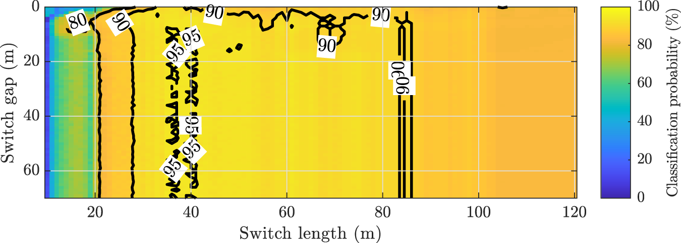
To analyze the observed misclassifications and assess sensitivity to switch length and spacing, a controlled simulation was conducted. All 63 switch signatures were extracted, resampled to common length, and augmented with mirrored duplicates to represent alternative orientations. Synthetic evaluation sequences with different switch lengths and inter-spacing (gap) were then formed by inserting the signatures into a simulated track background. The results in Fig. 10 report overall orientation classification accuracy without differentiating individual orientations, as no significant variation between classes was observed.
Simulation results showing the percentage of overall correct orientation classifications for varying switch lengths and gaps.

Figure 10 Long description
A heatmap illustrating classification probability as a percentage, with the x-axis labeled 'Switch length' in meters ranging from 0 to 120 and the y-axis labeled 'Switch gap' in meters ranging from 0 to 40. The color gradient represents classification probability from 0 to 100 percent, with specific values marked at various points: 80, 90, 95 and 90. The map shows varying probabilities across different combinations of switch length and gap, with higher probabilities indicated in certain regions.
Across the tested ranges, performance remained stable, indicating robustness to substantial deviations from the reference configuration. In closely spaced configurations, accuracy increased slightly, consistent with the contribution of contextual information captured by the circular variance. Compared to previous work [Reference Noll, Kohnert and Caldero1], where performance dropped sharply for gaps below  $40\,$m and switch lengths above $50\,$m, the proposed method demonstrates higher robustness. It also reduces complexity by removing both dynamic time warping (DTW) as an additional evaluation score and the $30\,$m observation window previously used for score evaluation. This simplification improves efficiency and robustness under streaming conditions but sacrifices peak performance, which previously exceeded $99\%$ within a narrow parameter region. When classification errors occur, they first appear at the same subset of closely interconnected switches observed in the real-world evaluation. Because spacing alone does not explain these failures, we attribute the remaining confusions primarily to altered feature patterns introduced by physical interconnections between adjacent switches, reinforcing the conclusions drawn from field experiments.
Conclusion
In this work, a novel method for detecting and classifying railway infrastructure elements, including switches, bridges with prominent metal components on the track surface, and overpasses, using multi-channel GPR was demonstrated. By leveraging statistical and structural features (energy, depth, and skewness) extracted from spatial B-scans, and combining pattern correlation with threshold-based decision-making in a streaming architecture, the proposed system enables detection and classification of typical trackside infrastructure, as well as switch orientation estimation, across a real-world railway network. The evaluation results demonstrate overall good performance for infrastructure detection and classification ( $98$–
$98$– $100\%$), with only minor misclassifications occurring for switch orientation estimation in scenarios involving closely spaced or physically interconnected switches ( $82$–
$82$– $100\%$), which were not represented in the reference dataset. Overall, the approach offers a promising candidate for landmark detection for enhancing train localization within train-localization frameworks by reducing distance drift at known infrastructure elements and limiting dependence on dedicated trackside hardware. Future work should extend the reference and evaluation datasets to cover additional infrastructure, such as more types of railroad switches and other rail superstructures. The approach needs to be integrated into a real-time localization framework, with additional state estimators implemented for online calibration to adapt to environmental changes and operational variability.
Competing interests
The authors are employees of Siemens Mobility GmbH. This research was conducted independently and is not related to any commercial product or service. The authors declare no competing interests.
AI use disclosure
GPT-4.1 was used for language polishing (grammar and clarity) only. No analysis, code, figures, results, or conclusions were generated by AI. AI is not an author.

Maximilian Noll received his M.Sc. degree in Electrical and Computer Engineering from the Technical University of Munich in 2020. He is currently an External Research Assistant at the Institute of Microwaves and Photonics at Friedrich-Alexander University Erlangen-Nürnberg and is employed at Siemens Mobility GmbH. His main research interests include ground-penetrating radar and railway localization.

Sören Kohnert was born in Rheda-Wiedenbrück, Germany, in 1991. He completed a double M.Eng. degrees in electrical engineering from Augsburg University of Applied Sciences, Germany, and Ulster University, United Kingdom, in 2017. In 2023, he earned his Ph.D. degree in electrical engineering from Ruhr University Bochum, Germany. He is currently employed as a Signal Processing Engineer at Siemens Mobility GmbH.

Pau Caldero was born in Barcelona, Spain, in 1992. He received his Ph.D. degree in Electrical Engineering from the Friedrich-Alexander-Universität Erlangen-Nürnberg (FAU) in 2023. He is currently working at Siemens Mobility GmbH in Munich, Germany. His research interests include signal processing, multi-sensor localization and perception, system architecture, and application development for next-generation mobility solutions and industrial automation.



 Open access

