





1. Introduction
Fluid flows, be it gas or liquid, can entrain and carry particles. The transport of a discrete, disperse phase is at play in various ways in a vast array of natural and everyday life phenomena (Woods Reference Woods2010), with examples ranging from cloud formation (Shaw Reference Shaw2003) to marine snow (Kiørboe Reference Kiørboe1997; Takeuchi et al. Reference Takeuchi, Doubell, Jackson, Yukawa, Sagara and Yamazaki2019), from sand storms to protoplanet formation. Furthermore, handling of disperse powders, dusts, grains and other suspensions is one of the cornerstones of modern industrial processing (Green & Perry Reference Green and Perry2008).
Disperse particles can be considered passively transported by the flow only in the case of small size, high dilution and low mass density (Brandt & Coletti Reference Brandt and Coletti2022), and in the absence of non-hydrodynamic field effects. Under these conditions, the particles have a negligible backreaction on the flow. In all other cases, however, particles do alter the flow field they occupy in fundamental ways (Balachandar & Eaton Reference Balachandar and Eaton2010; Marchioli, Rosti & Verhille Reference Marchioli, Rosti and Verhille2026). For example, they modulate flow structures, inducing turbulence enhancement or attenuation depending on their size (Elghobashi & Truesdell Reference Elghobashi and Truesdell1993; Elghobashi Reference Elghobashi1994; Oka & Goto Reference Oka and Goto2022; Olivieri, Cannon & Rosti Reference Olivieri, Cannon and Rosti2022), they are known to accumulate on walls in channel flows – a phenomenon known as turbophoresis – and thus disrupt the generation of vortical structures, effectively altering the production of turbulent kinetic energy (Battista et al. Reference Battista, Mollicone, Gualtieri, Messina and Casciola2019; Costa, Brandt & Picano Reference Costa, Brandt and Picano2021).
1.1. Particle settling
The presence of gravity instils additional complexity in particle behaviour. Early theoretical and experimental results by Richardson & Zaki (Reference Richardson and Zaki1954) revealed that semi-dilute and dense suspensions of particles (volume fraction $\varPhi _V\geqslant 0.05$
) settling in the Stokes regime show hindered mean settling speeds compared with the case of a single particle, due to the upward volume flux generated by the displaced fluid. Their study provided the empirical Richardson–Zaki relationship, which relates the hindered settling velocity of the particle suspension to the settling velocity of the single particle
$\varPhi _V\geqslant 0.05$
) settling in the Stokes regime show hindered mean settling speeds compared with the case of a single particle, due to the upward volume flux generated by the displaced fluid. Their study provided the empirical Richardson–Zaki relationship, which relates the hindered settling velocity of the particle suspension to the settling velocity of the single particle $v_t$
and the suspension’s occupied volume fraction in the form of a power law of the void fraction
$v_t$
and the suspension’s occupied volume fraction in the form of a power law of the void fraction $(1-\varPhi _V)$
, with an exponent dependent on the Reynolds number associated with the single particle’s terminal velocity
$(1-\varPhi _V)$
, with an exponent dependent on the Reynolds number associated with the single particle’s terminal velocity $ \textit{Re}_{t}$
. Later studies improved on this relationship by obtaining a better formulation for the exponent (Garside & Al-Dibouni Reference Garside and Al-Dibouni1977) and by including adequate prefactors (Di Felice Reference Di Felice1999; Yin & Koch Reference Yin and Koch2007) to better match the results at intermediate
$ \textit{Re}_{t}$
. Later studies improved on this relationship by obtaining a better formulation for the exponent (Garside & Al-Dibouni Reference Garside and Al-Dibouni1977) and by including adequate prefactors (Di Felice Reference Di Felice1999; Yin & Koch Reference Yin and Koch2007) to better match the results at intermediate $ \textit{Re}_{t}$
and higher dilution.
$ \textit{Re}_{t}$
and higher dilution.
The presence of velocity fluctuations in the fluid field, however, has been shown to alter this picture in complex ways. Already within the one-way coupled, linear drag limit, numerical studies beginning with Maxey (Reference Maxey1987) found that inertial particles in a turbulent flow settle faster than the same particle in quiescent flow or than an equivalent, non-inertial particle in the same turbulent flow. Maxey attributed this phenomenon to the preferential sampling by the particle of the high strain and low vorticity regions, producing a bias that affects the terminal velocity. More recent studies have challenged the view that enhanced settling speeds are only a by-product of the preferential sampling (Tom & Bragg Reference Tom and Bragg2019), and have highlighted that preferential sampling of the flow from the particles occurs at a range of scales that is dependent on the magnitude of particle inertia. This multiscale nature of the mechanisms influencing preferential sweeping was noted also in the experimental work by Petersen, Baker & Coletti (Reference Petersen, Baker and Coletti2019). The effect of turbulence on particles larger than the Kolmogorov scale has been less investigated. Fornari, Picano & Brandt (Reference Fornari, Picano and Brandt2016), in partial reproduction of the experimental work of Byron (Reference Byron2015), numerically studied semi-dilute suspensions ( $\varPhi _V=0.005$
–
$\varPhi _V=0.005$
– $0.01$
) of almost neutrally buoyant particles (solid-to-fluid density ratio
$0.01$
) of almost neutrally buoyant particles (solid-to-fluid density ratio $\rho _{p}/\rho _{\kern-1pt f}=1.02$
) in both quiescent and turbulent environments. Their results highlight that, in these conditions, reduction in terminal velocity when compared with
$\rho _{p}/\rho _{\kern-1pt f}=1.02$
) in both quiescent and turbulent environments. Their results highlight that, in these conditions, reduction in terminal velocity when compared with $v_t$
occurs for both quiescent and turbulent flows, in agreement with the experiments. They note how the magnitude of the settling hindrance is affected by the suspension’s microstructure, which also Yin & Koch (Reference Yin and Koch2007) find to be important at intermediate values of
$v_t$
occurs for both quiescent and turbulent flows, in agreement with the experiments. They note how the magnitude of the settling hindrance is affected by the suspension’s microstructure, which also Yin & Koch (Reference Yin and Koch2007) find to be important at intermediate values of $ \textit{Re}_{t}$
. Both works suggest that lower reductions in settling speeds are achieved due to intermittent events associated with draft-kissing-tumbling behaviour induced by particle wakes. Overall, studies with large particles have mostly found reductions in settling speeds when compared with
$ \textit{Re}_{t}$
. Both works suggest that lower reductions in settling speeds are achieved due to intermittent events associated with draft-kissing-tumbling behaviour induced by particle wakes. Overall, studies with large particles have mostly found reductions in settling speeds when compared with $v_t$
(Peng et al. Reference Peng, Karzhaubayev, Wang, Chen and Niu2025) or modest increases, depending on turbulence intensity (Chouippe & Uhlmann Reference Chouippe and Uhlmann2019).
$v_t$
(Peng et al. Reference Peng, Karzhaubayev, Wang, Chen and Niu2025) or modest increases, depending on turbulence intensity (Chouippe & Uhlmann Reference Chouippe and Uhlmann2019).
When considering large particles, however, background turbulence is not the only mechanism influencing the flow, and the particle-scale momentum injection can affect the observed dynamics. Even in dilute conditions, heavy particles settling in still fluid can show enhanced settling speeds due to higher ${Re}_t$
wake effects. In a pioneering work on the topic, Kajishima & Takiguchi (Reference Kajishima and Takiguchi2002) investigated numerically the settling in a triperiodic box of a semi-dilute suspension (
${Re}_t$
wake effects. In a pioneering work on the topic, Kajishima & Takiguchi (Reference Kajishima and Takiguchi2002) investigated numerically the settling in a triperiodic box of a semi-dilute suspension ( $\varPhi _V=0.002$
) of heavy (
$\varPhi _V=0.002$
) of heavy ( $\rho _p/\rho _{\kern-1pt f} = 8.8$
) particles at
$\rho _p/\rho _{\kern-1pt f} = 8.8$
) particles at ${Re}_t=50$
–
${Re}_t=50$
– $400$
. They observed columnar clustering of particles induced by wake effects. The presence of these clusters enhanced the settling speed when compared with
$400$
. They observed columnar clustering of particles induced by wake effects. The presence of these clusters enhanced the settling speed when compared with $v_t$
by creating preferential avenues of descending flow. In a following work, Kajishima (Reference Kajishima2004) noticed under similar conditions (
$v_t$
by creating preferential avenues of descending flow. In a following work, Kajishima (Reference Kajishima2004) noticed under similar conditions ( ${Re}_t = 300$
,
${Re}_t = 300$
, $\varPhi _V = 0.0005$
–
$\varPhi _V = 0.0005$
– $0.004$
,
$0.004$
, $\rho _p/\rho _{\kern-1pt f} = 8.8$
) that irrotational particles where absorbed into clusters, while rotational ones prevented their formation. Kajishima attributed this to a reversion in the direction of the lift induced by the shear caused by the falling particle column. In another landmark work, Uhlmann & Doychev (Reference Uhlmann and Doychev2014) expanded on the topic of columnar structures by simulating tall and slender fluid domains with
$\rho _p/\rho _{\kern-1pt f} = 8.8$
) that irrotational particles where absorbed into clusters, while rotational ones prevented their formation. Kajishima attributed this to a reversion in the direction of the lift induced by the shear caused by the falling particle column. In another landmark work, Uhlmann & Doychev (Reference Uhlmann and Doychev2014) expanded on the topic of columnar structures by simulating tall and slender fluid domains with $\mathcal{O}(10^4)$
heavy particles (
$\mathcal{O}(10^4)$
heavy particles ( $\rho _p/\rho _{\kern-1pt f} = 1.5$
) under dilute conditions (
$\rho _p/\rho _{\kern-1pt f} = 1.5$
) under dilute conditions ( $\varPhi _V = 0.005$
). They used two different values of the Galileo number (
$\varPhi _V = 0.005$
). They used two different values of the Galileo number ( $ \textit{Ga} = 121, 178$
) for which an equivalent particle in still fluid shows steady, axisymmetric wake or steady, planar-symmetric (oblique) wake, respectively. They observed the emergence of columnar particle clustering and enhanced settling speeds only for
$ \textit{Ga} = 121, 178$
) for which an equivalent particle in still fluid shows steady, axisymmetric wake or steady, planar-symmetric (oblique) wake, respectively. They observed the emergence of columnar particle clustering and enhanced settling speeds only for $ \textit{Ga}=178$
. They put forward the hypothesis that lateral motion may be responsible for the onset of clustering, which is then sustained by the draft generated by the descending particles’ wakes. The emergence of these columnar structures has been also confirmed by experimental studies (Huisman et al. Reference Huisman, Barois, Bourgoin, Chouippe, Doychev, Huck, Morales, Uhlmann and Volk2016). The settling of particles in quiescent flows remains a topic of active study. Recently, Jiang et al. (Reference Jiang, Brandt, Xu and Zhao2025) studied the settling of suspensions of spherical, oblate spheroidal and prolate spheroidal particles with
$ \textit{Ga}=178$
. They put forward the hypothesis that lateral motion may be responsible for the onset of clustering, which is then sustained by the draft generated by the descending particles’ wakes. The emergence of these columnar structures has been also confirmed by experimental studies (Huisman et al. Reference Huisman, Barois, Bourgoin, Chouippe, Doychev, Huck, Morales, Uhlmann and Volk2016). The settling of particles in quiescent flows remains a topic of active study. Recently, Jiang et al. (Reference Jiang, Brandt, Xu and Zhao2025) studied the settling of suspensions of spherical, oblate spheroidal and prolate spheroidal particles with $\varPhi _V=0.01$
,
$\varPhi _V=0.01$
, $ \textit{Ga}=80$
,
$ \textit{Ga}=80$
, $\rho _p/\rho _{\kern-1pt f}=2$
. They find settling such that spheroidal particles appear to form columnar clusters more readily, enhancing settling rates when compared with
$\rho _p/\rho _{\kern-1pt f}=2$
. They find settling such that spheroidal particles appear to form columnar clusters more readily, enhancing settling rates when compared with $v_t$
.
$v_t$
.
1.2. Transient settling with interface
As is true for the cases presented so far, the vast majority of the research efforts in the area of settling and clustering of particles has focused on phenomena emerging in (statistically) stationary solutions. The problem of the transient initiation of settling has faced less scrutiny, and this is especially true for studies involving finite-size particles. In this regard, the problem that steady-state settling studies circumvent is that of the initial configuration of the system. Different initial configurations can, however, fundamentally impact the development of the solution in practical instances. One example is that of turbidity currents (Meiburg & Kneller Reference Meiburg and Kneller2010; Xie & Pan Reference Xie and Pan2025). In this study, we concern ourselves with one such initial configuration, which is the transient settling of a heavy, semi-dilute particle-laden phase forming a planar interface with the unladen fluid below it. This particular configuration is analogous to the one giving rise to the Rayleigh–Taylor (RT) instability.
1.2.1. Rayleigh–Taylor configuration and instability
In the classic RT scenario, a heavier fluid is sitting atop a lighter one in the presence of an acceleration field, typically the gravitational one. The two fluids share a planar interface, which, at the start of the transient, is infinitesimally perturbed. This perturbation amplifies exponentially in time due to the growing misalignment of the pressure and density gradients across the interface. Linear stability analysis in the inviscid limit shows that the early stage growth rate of a single mode instability of wave number $k$
is equal to
$k$
is equal to $\lambda =\sqrt {Agk}$
(Kull Reference Kull1991). Here,
$\lambda =\sqrt {Agk}$
(Kull Reference Kull1991). Here, $A$
is the Atwood number, defined as
$A$
is the Atwood number, defined as $A = (\rho _{2}-\rho _{1} )/ (\rho _{2}+\rho _{1} )$
,
$A = (\rho _{2}-\rho _{1} )/ (\rho _{2}+\rho _{1} )$
, $g$
is the gravitational acceleration. When the amplitude of the instability reaches approximately one third of the wavelength, nonlinear effects start breaking up the interface, which ceases to be single valued. In this stage, the instability gives rise to mixing, in the form of characteristic ascending and descending plumes. If the flow is allowed to grow sufficiently energetic, turbulence sets in. Under the assumption of single-fluid, linear density variation (also known as the Oberbeck–Boussinesq (OB) approximation), the growth of the mixing zone height is proportional to
$g$
is the gravitational acceleration. When the amplitude of the instability reaches approximately one third of the wavelength, nonlinear effects start breaking up the interface, which ceases to be single valued. In this stage, the instability gives rise to mixing, in the form of characteristic ascending and descending plumes. If the flow is allowed to grow sufficiently energetic, turbulence sets in. Under the assumption of single-fluid, linear density variation (also known as the Oberbeck–Boussinesq (OB) approximation), the growth of the mixing zone height is proportional to $Agt^{2}$
, and Chertkov (Reference Chertkov2003) predicted a Kolmogorov–Obukhov scenario by introducing a quasistationary, adiabatic view of the evolution of the time-dependent cross-scale turbulent kinetic energy flux
$Agt^{2}$
, and Chertkov (Reference Chertkov2003) predicted a Kolmogorov–Obukhov scenario by introducing a quasistationary, adiabatic view of the evolution of the time-dependent cross-scale turbulent kinetic energy flux $\varepsilon (t)$
. A more detailed phenomenology of RT turbulence in the OB approximation has been reviewed by Boffetta & Mazzino (Reference Boffetta and Mazzino2017).
$\varepsilon (t)$
. A more detailed phenomenology of RT turbulence in the OB approximation has been reviewed by Boffetta & Mazzino (Reference Boffetta and Mazzino2017).
1.2.2. Particle-laden heavy phase
The case in which a particle-laden phase takes up the role of the top fluid (in the RT sense) has interested several communities across the scientific spectrum, since it arises in a wide set of geophysical and artificial flows, although often in combination with other effects. This set-up has been studied experimentally in the context of magma dynamics by Michioka & Sumita (Reference Michioka and Sumita2005), and with viscosity stratification by Thomas, Tait & Koyaguchi (Reference Thomas, Tait and Koyaguchi1993). It has been studied in the context of settling of aerosols (Hinds et al. Reference Hinds, Ashley, Kennedy and Bucknam2002), plankton transport (Green & Diez Reference Green and Diez1995), but also, in connection with electrodynamic effects, for dusty plasmas (D’Angelo Reference D’Angelo1993). A particular class of geophysical flows where this set-up is particularly relevant is that of sediment-rich riverine outflows. When sediment-rich fluvial water pours into the sea, stratification of particle-laden fresh water over salty ocean water can occur, producing an initial condition analogous to that of the particle-laden RT configuration. Because of the strong connection with this phenomenon, the majority of the studies focus on the coupled effect of salinity (or temperature) and particle concentration gradients, which leads it to be known broadly as double-diffusive sedimentation. The relatively modest body of literature in the field includes experimental (Houk & Green Reference Houk and Green1973; Green Reference Green1987; Chen Reference Chen1997; Hoyal, Bursik & Atkinson Reference Hoyal, Bursik and Atkinson1999; Parsons, Bush & Syvitski Reference Parsons, Bush and Syvitski2001; McCool & Parsons Reference McCool and Parsons2004; Rouhnia & Strom Reference Rouhnia and Strom2015; Sutherland et al. Reference Sutherland, Mueller, Sjerve and Deepwell2021), theoretical (Burns & Meiburg Reference Burns and Meiburg2012; Yu, Hsu & Balachandar Reference Yu, Hsu and Balachandar2013) and numerical (Yu, Hsu & Balachandar Reference Yu, Hsu and Balachandar2014; Burns & Meiburg Reference Burns and Meiburg2015; Hung, Niu & Chou Reference Hung, Niu and Chou2020) works. Taken as a whole, the literature is unanimous on the formation of plumes of particles, or fingers, that heighten the sedimentation rate compared with the single particle case, with the effect being generally more pronounced as the mass loading increases. The most recent works highlight the difference between two modes of settling: double-diffusion driven, or convective sedimentation driven, which is the RT case (Hoyal et al. Reference Hoyal, Bursik and Atkinson1999; Maxworthy Reference Maxworthy1999; Burns & Meiburg Reference Burns and Meiburg2012; Yu et al. Reference Yu, Hsu and Balachandar2013; Sutherland et al. Reference Sutherland, Mueller, Sjerve and Deepwell2021). A few numerical studies have investigated the phenomenon in the absence of any salinity or temperature gradient using both Euler–Euler (Chou, Wu & Shih Reference Chou, Wu and Shih2014) and point-particle models (Yamamoto, Hisataka & Harada Reference Yamamoto, Hisataka and Harada2015) under the assumption of Stokesian particle drag. Chou et al. (Reference Chou, Wu and Shih2014) showed a developed state of the instability, where the growth of the mixing zone is proportional to $t^{2}$
, similarly to the classic single-phase case. On the other hand, Yamamoto et al. (Reference Yamamoto, Hisataka and Harada2015) focused on the initial, laminar phase of the instability in a quasi-two-dimensional domain. They highlight an initially exponential growth of the width of mixing, which then settles onto linear at later times. In both cases, the suspensions are dilute, and as such hindrance effects are generally negligible.
$t^{2}$
, similarly to the classic single-phase case. On the other hand, Yamamoto et al. (Reference Yamamoto, Hisataka and Harada2015) focused on the initial, laminar phase of the instability in a quasi-two-dimensional domain. They highlight an initially exponential growth of the width of mixing, which then settles onto linear at later times. In both cases, the suspensions are dilute, and as such hindrance effects are generally negligible.
Other studies have focused on the instability in the context of both liquid–solid (Völtz et al. Reference Völtz, Schröter, Iori, Betat, Lange, Engel and Rehberg2000, Reference Völtz, Pesch and Rehberg2001) and gas–solid (Vinningland et al. Reference Vinningland, Johnsen, Flekkøy, Toussaint and Måløy2007, Reference Vinningland, Johnsen, Flekkøy, Toussaint and Måløy2010) experiments using Hele-Shaw cells. In these works, the heavy particle-laden phase is obtained through the sedimentation of particles in the cell, and the instability is initiated upon its rotation. In their experiments, Völtz et al. (Reference Völtz, Schröter, Iori, Betat, Lange, Engel and Rehberg2000, Reference Völtz, Pesch and Rehberg2001) make use of hindered settling to obtain an initial particle-laden phase volume fractions of around 6.5 %. They focus on the growth rate of different instability modes, showing a non-monotonic dependency on the wavenumber. In the work of Vinningland et al. (Reference Vinningland, Johnsen, Flekkøy, Toussaint and Måløy2007, Reference Vinningland, Johnsen, Flekkøy, Toussaint and Måløy2010), the sedimentation procedure leads to an initial close packing of the particle-laden phase due to the diminished buoyancy, and the shape of the finger-like patterns is starkly different from that of the liquid–solid case: the granules arrange in cusp-shaped, almost filamentous structures. The analysis of both experiments and simulations shows the scale invariance of the instability in the ${70}\,{}\, \textrm {to}\, {570}\,{\mu }{\textrm {m}}$
range of particle diameters sizes.
${70}\,{}\, \textrm {to}\, {570}\,{\mu }{\textrm {m}}$
range of particle diameters sizes.
Pan, Joseph & Glowinski (Reference Pan, Joseph and Glowinski2001) performed two-dimensional simulations of a sedimenting solid–liquid suspension of cylinders at high packing fraction in the RT configuration, using the method of distributed Lagrangian multipliers. In the work, they focus their attention on the initial instability of the particle front, and model the instability by using a two-fluid model that describes the particle-laden phase as a heavier-than-water fluid with an effective density and viscosity. They find that the effective viscosity depends on the geometrical parameters of the domain. Additionally, they stress the dependence of the viscosity on the lattice arrangement of the cylinders, even when studying the instability in the limit of infinite domain, finding significant differences across rectangular, hexagonal and random initial configurations.
In most of these studies, the fundamental assumption of small particles in Stokesian regime is used. For Euler–Euler models this constraint is inherent: the deviation of particles from streamlines due to finite inertia can cause the emergence of caustics (i.e. particles with very different velocities in nearby locations). This behaviour cannot be captured by a Eulerian field that has to stay locally single valued. Nonetheless, since caustic formation increases exponentially with the particles Stokes number $St$
, weak inertial effects can be accounted for. Based on this consideration, Magnani, Musacchio & Boffetta (Reference Magnani, Musacchio and Boffetta2021) investigated the effect of weak particle inertia on RT turbulence using the model by Saffman (Reference Saffman1962), which models particles as infinitesimal in size, but with finite inertia. Their analysis shows that, in the limit of vanishingly small Stokes time, particle-laden RT turbulence recovers the classic OB limit with similar phenomenology, including a long-time
$St$
, weak inertial effects can be accounted for. Based on this consideration, Magnani, Musacchio & Boffetta (Reference Magnani, Musacchio and Boffetta2021) investigated the effect of weak particle inertia on RT turbulence using the model by Saffman (Reference Saffman1962), which models particles as infinitesimal in size, but with finite inertia. Their analysis shows that, in the limit of vanishingly small Stokes time, particle-laden RT turbulence recovers the classic OB limit with similar phenomenology, including a long-time $t^2$
mixing layer growth rate. However, higher Stokes time can induce symmetry-breaking effects in the mixing layer density profile and delay the development of turbulent mixing. Additionally, this inertial dynamic is observed to lead to the formation of clusters with higher-than-initial particle concentration, which is a phenomenon that cannot be achieved in the standard OB limit.
$t^2$
mixing layer growth rate. However, higher Stokes time can induce symmetry-breaking effects in the mixing layer density profile and delay the development of turbulent mixing. Additionally, this inertial dynamic is observed to lead to the formation of clusters with higher-than-initial particle concentration, which is a phenomenon that cannot be achieved in the standard OB limit.
A class of particle-laden flow models that are generally applicable to dense, high-inertia particle-laden flows is available. These models, generally referred to as two-fluid models, introduce a balance equation for the fluctuating velocity component of the particle phase (Fox Reference Fox2014; Rauchenzauner & Schneiderbauer Reference Rauchenzauner and Schneiderbauer2020). However, due to their departure from the low-Stokes, high-dilution conditions, these models require additional closures which are generally obtained from numerical simulations. Existing closures are derived from the statistical analysis of steady-state, homogeneous systems, so that the extent to which they may be applicable to the particle-laden RT set-up is unclear. Additionally, two-fluid models are known to behave poorly in the presence of sharp gradients of volume fraction, a conditions that is especially relevant for the RT initial configuration. Possibly as a consequence of the reasons above, to the authors’ knowledge there appear to be no studies that use two-fluid models to investigate the particle-laden RT configuration.
1.3. Present work
The limitations of the available particle-phase models have left the role of strong inertia and that of displaced-fluid volume flux unaccounted for. In order to overcome these limitations and study the effect of these parameters, we numerically investigate the particle RT set-up using heavy, finite-size particles at non-negligible dilution, which was achieved numerically through the use of direct numerical simulation (DNS) and a fully coupled immersed boundary method (IBM). A global description of the system phenomenology is presented in our recent work (Tandurella et al. Reference Tandurella, Rosti, Musacchio and Boffetta2026): as in the classic RT case, we observed the generation of a leading mixing layer and a trailing bulk region of uniform particle concentration; however, in departure from the two-fluid scenario, we found that the mixing layer expands with an anomalous, non-integer exponent. We observed this dynamic to be superimposed over an average settling drift of the particles, and recovered a simplified, one-dimensional model of the system which accurately described the evolution of the particle concentration across different values of inertia.
In the present work, we further our analysis of this system. Using the same set-up, we expand our investigations to include fluid and particle statistics and relate them to local quantities. We give insight on the generation of the interfacial instability and on the effect of turbulence within the two flow regions. Further observations of the global system behaviour are also included.
The remainder of this manuscript is divided in the following sections: in § 2 we present in detail the set-up and numerical methods that were used for the investigation, while in § 3 we present and discuss the results of the study. More specifically, in § 3.1 we give a brief overview of the system and recall the previous results; then, we present additional global observations: in § 3.2 we discuss turbulence statistics for the mixing and bulk regions, in § 3.3 we focus more closely on the dynamics of the particles and in § 3.4 we investigate their mutual interaction with flow structures. Finally, we compile our conclusions in § 4.
2. Simulation set-up
2.1. Set-up
In order to investigate the proposed system, we perform a series of numerical simulations. The set-up consists of $n_{p}={100\,000}$
spherical particles initialised in a uniformly random, non-overlapping fashion in the top half of a vertical box domain of dimensions
$n_{p}={100\,000}$
spherical particles initialised in a uniformly random, non-overlapping fashion in the top half of a vertical box domain of dimensions $L_{x}\times L_{y} \times L_{z} = 2\pi \times 2\pi \times 8\pi$
. The diameter of the particles is fixed (
$L_{x}\times L_{y} \times L_{z} = 2\pi \times 2\pi \times 8\pi$
. The diameter of the particles is fixed ( $d_{p}={0.0982}$
) in order to obtain an analytical solid volume fraction
$d_{p}={0.0982}$
) in order to obtain an analytical solid volume fraction $\phi _{b} \approx {0.1}$
in the particle-filled portion of the domain. A
$\phi _{b} \approx {0.1}$
in the particle-filled portion of the domain. A $z$
-aligned body force
$z$
-aligned body force $\rho g$
is imposed on both fluid and solids, with
$\rho g$
is imposed on both fluid and solids, with $g=1$
kept constant and the density
$g=1$
kept constant and the density $\rho$
set as a material property –
$\rho$
set as a material property – $\rho _{\kern-1pt f}$
and
$\rho _{\kern-1pt f}$
and $\rho _{p}$
for the fluid and solid phases, respectively. Four different ratios of particle-to-fluid density
$\rho _{p}$
for the fluid and solid phases, respectively. Four different ratios of particle-to-fluid density $\gamma = \rho _{p} / \rho _{\kern-1pt f} = \{ 2,4,8,16 \}$
have been investigated in order to focus the study on the role of particle inertia, while the fluid kinematic viscosity
$\gamma = \rho _{p} / \rho _{\kern-1pt f} = \{ 2,4,8,16 \}$
have been investigated in order to focus the study on the role of particle inertia, while the fluid kinematic viscosity $\nu =0.002$
is kept constant. Based on the chosen values of the parameters, the obtained
$\nu =0.002$
is kept constant. Based on the chosen values of the parameters, the obtained $\textit {Ga}$
,
$\textit {Ga}$
, $\textit {A}$
and
$\textit {A}$
and $ \textit{Re}_t$
– which vary with
$ \textit{Re}_t$
– which vary with $\gamma$
– are defined and reported in table 1.
$\gamma$
– are defined and reported in table 1.
Corresponding values of non-dimensional quantities for the values of $\gamma$
investigated.
$\gamma$
investigated. $\textit {A}=(\rho _2-\rho _1)/(\rho _2+\rho _1)$
, where
$\textit {A}=(\rho _2-\rho _1)/(\rho _2+\rho _1)$
, where $\rho _2=\rho _{p}\phi _{b}+\rho _{\kern-1pt f}(1-\phi _{b})$
and
$\rho _2=\rho _{p}\phi _{b}+\rho _{\kern-1pt f}(1-\phi _{b})$
and $\rho _1=\rho _{\kern-1pt f}$
. Here,
$\rho _1=\rho _{\kern-1pt f}$
. Here, $\textit {Ga}=\sqrt {(\gamma -1)d_{p} g}d_{p}/\nu$
and
$\textit {Ga}=\sqrt {(\gamma -1)d_{p} g}d_{p}/\nu$
and $ \textit{Re}_t=|v_t|d_{p}/\nu$
, where
$ \textit{Re}_t=|v_t|d_{p}/\nu$
, where $v_t(\gamma )$
is the sedimentation velocity of a single particle (reported in Appendix C).
$v_t(\gamma )$
is the sedimentation velocity of a single particle (reported in Appendix C).

Periodic boundary conditions are imposed on the $x$
and
$x$
and $y$
aligned faces of the domain. At the top and bottom of the domain, the no-slip and no-penetration conditions are set. For the results that concern the mixing region between the two phases, we are interested only in the dynamics far from the walls. Because of this, our analyses are constrained to the flow region in the range
$y$
aligned faces of the domain. At the top and bottom of the domain, the no-slip and no-penetration conditions are set. For the results that concern the mixing region between the two phases, we are interested only in the dynamics far from the walls. Because of this, our analyses are constrained to the flow region in the range $0.2 L_{z} \leqslant z \leqslant 0.8 L_{z}$
. Careful analysis of our data and a validation simulation performed with a taller domain (see Appendix B) has convinced us that this distance is conservative enough to prevent unwanted influence of the top and bottom boundaries.
$0.2 L_{z} \leqslant z \leqslant 0.8 L_{z}$
. Careful analysis of our data and a validation simulation performed with a taller domain (see Appendix B) has convinced us that this distance is conservative enough to prevent unwanted influence of the top and bottom boundaries.
To understand the robustness of global features upon variation of particle concentration, two sets of additional simulations were performed using different initial volume fractions $\phi _{b}=0.05, 0.15$
for the
$\phi _{b}=0.05, 0.15$
for the $\gamma =2, 8$
cases.
$\gamma =2, 8$
cases.
2.2. Numerical methods
We perform DNS by time integrating a discretised version of the full Navier–Stokes equations
 \begin{align} \frac {\partial \boldsymbol{u}}{\partial t} + \boldsymbol{u} \boldsymbol{\cdot }\boldsymbol{\nabla } \boldsymbol{u} = - \frac {\boldsymbol{\nabla } p}{\rho _{\kern-1pt f}} + \nu {\nabla }^2 \boldsymbol{u} + \boldsymbol{f}^{{pf}}, \\[-28pt] \nonumber \end{align}
 \begin{align} \boldsymbol{\nabla } \boldsymbol{\cdot }\boldsymbol{u} = 0 , \\[0pt] \nonumber \end{align}
where $\boldsymbol{u}=(u_x,u_y,u_z)$
is the fluid velocity,
$\boldsymbol{u}=(u_x,u_y,u_z)$
is the fluid velocity, $p$
is the pressure and
$p$
is the pressure and $\boldsymbol{f}^{{pf}}$
is the fluid–solid coupling. In particular, the flow domain is discretised with
$\boldsymbol{f}^{{pf}}$
is the fluid–solid coupling. In particular, the flow domain is discretised with $384\times 384\times 1536$
Cartesian nodes and solved using the parallel DNS incompressible fluid solver Fujin, co-developed by the Complex Fluids and Flows unit at the Okinawa Institute of Science and Technology (Rosti Reference Rosti2026). It features a second-order central finite difference scheme in space and second-order Adams–Bashforth scheme in time. The incompressibility constraint is enforced through a fractional step method. The flow is forced solely by the particles, whose motion is computed according to the Newton–Euler equations of motion for rigid spheres
$384\times 384\times 1536$
Cartesian nodes and solved using the parallel DNS incompressible fluid solver Fujin, co-developed by the Complex Fluids and Flows unit at the Okinawa Institute of Science and Technology (Rosti Reference Rosti2026). It features a second-order central finite difference scheme in space and second-order Adams–Bashforth scheme in time. The incompressibility constraint is enforced through a fractional step method. The flow is forced solely by the particles, whose motion is computed according to the Newton–Euler equations of motion for rigid spheres
 \begin{align} m_{p} \frac {\text{d} \boldsymbol{v}}{\text{d} t} = \boldsymbol{f}_{\kern-1pt g} + \boldsymbol{f}^{{fp}} + \boldsymbol{f}_{\kern-1pt p}^{{pp}}, \\[-28pt] \nonumber \end{align}
 \begin{align} I_{p} \frac {\text{d} \boldsymbol{\omega }_p}{\text{d} t} = \boldsymbol{L}_p^{{fp}} . \\[0pt] \nonumber \end{align}
Here, $m_{p} = \rho _{p} V_{p} = \rho _{p} \pi d_{p}^3/6$
is the particle’s mass and
$m_{p} = \rho _{p} V_{p} = \rho _{p} \pi d_{p}^3/6$
is the particle’s mass and $I_{p} = m_{p} d_{p}^2/10$
is its moment of inertia,
$I_{p} = m_{p} d_{p}^2/10$
is its moment of inertia, $\boldsymbol{v}$
and
$\boldsymbol{v}$
and $\boldsymbol{\omega }_p$
are the particle’s translational and rotational velocities,
$\boldsymbol{\omega }_p$
are the particle’s translational and rotational velocities, $\boldsymbol{f}_{\kern-1pt g} = - (\gamma -1 ) \rho _{\kern-1pt f} V_{p} g \boldsymbol{e}_z$
is the gravitational (and buoyancy) force,
$\boldsymbol{f}_{\kern-1pt g} = - (\gamma -1 ) \rho _{\kern-1pt f} V_{p} g \boldsymbol{e}_z$
is the gravitational (and buoyancy) force, $\boldsymbol{f}^{{pp}}$
is the force due to particle collisions, while
$\boldsymbol{f}^{{pp}}$
is the force due to particle collisions, while $\boldsymbol{f}^{{fp}}$
and
$\boldsymbol{f}^{{fp}}$
and $\boldsymbol{L}_p^{{fp}}$
are the forces and torques due to the fluid–solid interaction
$\boldsymbol{L}_p^{{fp}}$
are the forces and torques due to the fluid–solid interaction
 \begin{align} \boldsymbol{f}^{{fp}} = \oint _{\partial V_p} \boldsymbol{\sigma } \boldsymbol{\cdot }\boldsymbol{n} \text{d}A, \\[-28pt] \nonumber \end{align}
 \begin{align} \boldsymbol{L}_p^{{fp}} = \oint _{\partial V_p} \boldsymbol{r} \times \left ( \boldsymbol{\sigma } \boldsymbol{\cdot }\boldsymbol{n} \right ) \text{d} A, \\[0pt] \nonumber \end{align}
where $\boldsymbol{\sigma }= -p \mathcal{I} + 2 \mu \mathcal{D}$
is the Cauchy stress tensor, with
$\boldsymbol{\sigma }= -p \mathcal{I} + 2 \mu \mathcal{D}$
is the Cauchy stress tensor, with $\mathcal{I}$
being the identity tensor,
$\mathcal{I}$
being the identity tensor, $\mu =\rho _{\kern-1pt f} \nu$
the fluid viscosity,
$\mu =\rho _{\kern-1pt f} \nu$
the fluid viscosity, $\mathcal{D}$
the strain rate tensor and
$\mathcal{D}$
the strain rate tensor and $\boldsymbol{n}$
the unit vector normal to the surface of the particle. The fluid–solid and solid–solid coupling are performed through the use of the Eulerian IBM by Hori, Rosti & Takagi (Reference Hori, Rosti and Takagi2022), which includes a soft-sphere collision model (Cundall & Strack Reference Cundall and Strack1979) and implicit lubrication. This method and the solver it is included in have been thoroughly validated (Rosti Reference Rosti2026, https://www.oist.jp/research/research-units/cffu/validation) and have been extensively used in previous works (Olivieri et al. Reference Olivieri, Cannon and Rosti2022; Chiarini & Rosti Reference Chiarini and Rosti2024; Chiarini, Tandurella & Rosti Reference Chiarini, Tandurella and Rosti2025). We note that, despite the relatively high volume fraction, in the range of
$\boldsymbol{n}$
the unit vector normal to the surface of the particle. The fluid–solid and solid–solid coupling are performed through the use of the Eulerian IBM by Hori, Rosti & Takagi (Reference Hori, Rosti and Takagi2022), which includes a soft-sphere collision model (Cundall & Strack Reference Cundall and Strack1979) and implicit lubrication. This method and the solver it is included in have been thoroughly validated (Rosti Reference Rosti2026, https://www.oist.jp/research/research-units/cffu/validation) and have been extensively used in previous works (Olivieri et al. Reference Olivieri, Cannon and Rosti2022; Chiarini & Rosti Reference Chiarini and Rosti2024; Chiarini, Tandurella & Rosti Reference Chiarini, Tandurella and Rosti2025). We note that, despite the relatively high volume fraction, in the range of $\gamma$
(and thus
$\gamma$
(and thus $\textit {St}$
) investigated, particle–particle collisions were observed not to play any meaningful role.
$\textit {St}$
) investigated, particle–particle collisions were observed not to play any meaningful role.
Based on the discretisation used and on the parameters described in the set-up of the problem, a ratio of particle diameter to grid node spacing $d_{p}/\Delta x = 6$
is obtained. To understand the impact of this grid on the results, tests of convergence upon variation of the resolution were performed for the main quantities of interest for the study, with the results reported in Appendix A showing satisfactory convergence.
$d_{p}/\Delta x = 6$
is obtained. To understand the impact of this grid on the results, tests of convergence upon variation of the resolution were performed for the main quantities of interest for the study, with the results reported in Appendix A showing satisfactory convergence.
In order to improve statistical convergence, for each of the different $\gamma$
tested, 3 different realisations of the flows using the same set of 3 random initial particle distributions were performed. The results presented in this work are then obtained by performing ensemble averages across said realisations.
$\gamma$
tested, 3 different realisations of the flows using the same set of 3 random initial particle distributions were performed. The results presented in this work are then obtained by performing ensemble averages across said realisations.
3. Results
3.1. Overview
Volumetric rendering of the instantaneous vertical velocity field $u_z(\boldsymbol{x})$
at
$u_z(\boldsymbol{x})$
at $t/\tau _t=0.02, 0.10, 0.17, 0.25$
for the case with
$t/\tau _t=0.02, 0.10, 0.17, 0.25$
for the case with $\gamma =2$
. Regions of low velocity magnitude are rendered as transparent, while large negative and large positive values are represented using blue and red areas, respectively. Time advancement is represented clockwise.
$\gamma =2$
. Regions of low velocity magnitude are rendered as transparent, while large negative and large positive values are represented using blue and red areas, respectively. Time advancement is represented clockwise.

Development of the interfacial instability, visualised from the bottom view of figure 1. Time advancement is from (a) to (d).

We start the analysis of our results through a qualitative description of the system phenomenology, using for reference a visualisation obtained from one of the repetitions of the $\gamma =2$
simulation set, figure 1. At time
$\gamma =2$
simulation set, figure 1. At time $t=0$
, the initial interface between the particle-laden and unladen phases is approximately flat, with only small-scale noise of the order of the average particle spacing due to the random particle placement. Past
$t=0$
, the initial interface between the particle-laden and unladen phases is approximately flat, with only small-scale noise of the order of the average particle spacing due to the random particle placement. Past $t=0$
, the particle suspension begins to fall in the gravitational direction. The settling front, however, does not advance homogeneously and the small-wavelength noise of the particle-laden phase causes localised misalignments of the pressure and density gradients. These misalignments cause the emergence of a net torques across the interface, which in turn further increase misalignment, in a feedback loop. As a result, plumes of particles start to appear in the interfacial region, with their wavelength and amplitude growing in time, generating mixing between the laden and unladen phases (figure 2). While this dynamic is especially visible for the particle-laden phase, corresponding plumes of unladen fluid also make their way through the particles. The interpenetration and mixing of the two phases, which is fundamentally driven by volume conservation, bears resemblance to the classic two-fluid RT instability. Above the interfacial region, the unmixed particle-laden phase also settles, leaving behind unladen fluid. The flow in this region presents a different phenomenology compared with that of the interface, marked by a more homogeneous particle distribution. Velocity fluctuations at scales larger that the particle one remain nonetheless present.
$t=0$
, the particle suspension begins to fall in the gravitational direction. The settling front, however, does not advance homogeneously and the small-wavelength noise of the particle-laden phase causes localised misalignments of the pressure and density gradients. These misalignments cause the emergence of a net torques across the interface, which in turn further increase misalignment, in a feedback loop. As a result, plumes of particles start to appear in the interfacial region, with their wavelength and amplitude growing in time, generating mixing between the laden and unladen phases (figure 2). While this dynamic is especially visible for the particle-laden phase, corresponding plumes of unladen fluid also make their way through the particles. The interpenetration and mixing of the two phases, which is fundamentally driven by volume conservation, bears resemblance to the classic two-fluid RT instability. Above the interfacial region, the unmixed particle-laden phase also settles, leaving behind unladen fluid. The flow in this region presents a different phenomenology compared with that of the interface, marked by a more homogeneous particle distribution. Velocity fluctuations at scales larger that the particle one remain nonetheless present.
Definitions of $z_0$
,
$z_0$
, $z_1$
and
$z_1$
and $z_2$
on the basis of the plane-averaged particle volume fraction
$z_2$
on the basis of the plane-averaged particle volume fraction $\langle \phi \rangle _{xy}(z,t)$
. The same four values of non-dimensional time
$\langle \phi \rangle _{xy}(z,t)$
. The same four values of non-dimensional time $t/\tau _t$
of figure 1 are presented for the case with
$t/\tau _t$
of figure 1 are presented for the case with $\gamma =2$
. The curves on the right show the instantaneous
$\gamma =2$
. The curves on the right show the instantaneous $\langle \phi \rangle _{xy}$
for the snapshots depicted on the left. For
$\langle \phi \rangle _{xy}$
for the snapshots depicted on the left. For $t/\tau _t=0.25$
, dashed lines are shown as a visual aid for the definition of the mixing layer and bulk boundaries. To simplify the visualisation, a 33 grid points coarse graining stencil is applied to the particle concentration profiles.
$t/\tau _t=0.25$
, dashed lines are shown as a visual aid for the definition of the mixing layer and bulk boundaries. To simplify the visualisation, a 33 grid points coarse graining stencil is applied to the particle concentration profiles.

Figure 3. Long description
Panel A: The first panel shows a series of four visualizations depicting the distribution of particles within a fluid flow at different non-dimensional times. The particles are represented in various colors, indicating different concentrations. Panel B: The second panel is a line graph showing the instantaneous plane-averaged particle volume fraction profiles corresponding to the snapshots in Panel A. The x-axis represents the normalized height (z/Lz), and the y-axis represents the normalized particle volume fraction (phi_xy(z,t)/phib). The graph includes four lines, each representing a different non-dimensional time value (0.02, 0.10, 0.17, 0.25). Dashed lines are used as visual aids to define the mixing layer and bulk boundaries. The graph is simplified using a 33 grid points coarse graining stencil applied to the particle concentration profiles.
The plane-averaged particle volume fraction profile $\langle \phi \rangle _{xy} (z,t )$
(figure 3 for
$\langle \phi \rangle _{xy} (z,t )$
(figure 3 for $\gamma =2$
) reflects the presence of the two main particle-laden regions in the flow: one at the advancing front where the profile expands in an approximately linear fashion, and one just above it where the profile is constant. The presence of this relatively sharp discontinuity between the two zones lends to their identification as separate regions of the flow. As proposed in Tandurella et al. (Reference Tandurella, Rosti, Musacchio and Boffetta2026), in order to identify the two unambiguously we fit the concentration profile with a piecewise linear function
$\gamma =2$
) reflects the presence of the two main particle-laden regions in the flow: one at the advancing front where the profile expands in an approximately linear fashion, and one just above it where the profile is constant. The presence of this relatively sharp discontinuity between the two zones lends to their identification as separate regions of the flow. As proposed in Tandurella et al. (Reference Tandurella, Rosti, Musacchio and Boffetta2026), in order to identify the two unambiguously we fit the concentration profile with a piecewise linear function
 \begin{align} \phi (z,t) = \left \{ \begin{array}{ll} 0 & z \leqslant z_0 \land z \gt z_2 ,\\[5pt]\phi _{b} \frac {z-z_0}{z_1-z_0} & z_0 \leqslant z \leqslant z_2 ,\\[5pt]\phi _{b} & z_1 \leqslant z \leqslant z_2.\\ \end{array} \right . \end{align}
Accordingly, we define the region of space delimited by $z_0(t) \leqslant z \leqslant z_2(t)$
as the mixing layer and that delimited by
$z_0(t) \leqslant z \leqslant z_2(t)$
as the mixing layer and that delimited by $z_1(t) \leqslant z \leqslant z_2(t)$
as the bulk. This procedure is visually represented in figure 3.
$z_1(t) \leqslant z \leqslant z_2(t)$
as the bulk. This procedure is visually represented in figure 3.
Locations of top, bottom (continuous lines) and geometric centre (dashed line) of the mixing layer and bulk in time, normalised for the simulation constant time scale $\tau$
(a),
$\tau$
(a), $\tau _g$
(b) and
$\tau _g$
(b) and $\tau _t$
(c). For case
$\tau _t$
(c). For case $\gamma =2$
, timestamps for the fields presented in figure 1 are also shown using triangular markers on the time axis.
$\gamma =2$
, timestamps for the fields presented in figure 1 are also shown using triangular markers on the time axis.

Based on this definition, we visualise the time evolution of $z_0(t)$
,
$z_0(t)$
, $z_1(t)$
,
$z_1(t)$
, $z_2(t)$
for all values of
$z_2(t)$
for all values of $\gamma$
in figure 4. Additionally, we report the location of the mixing layer geometric centre
$\gamma$
in figure 4. Additionally, we report the location of the mixing layer geometric centre $z_c=(z_0+z_1)/2$
. The diverging paths of
$z_c=(z_0+z_1)/2$
. The diverging paths of $z_0$
and
$z_0$
and $z_1$
represents the mixing layer expansion, while the progressive drift of the entire particle-laden phase is evidenced by the downward trajectory of
$z_1$
represents the mixing layer expansion, while the progressive drift of the entire particle-laden phase is evidenced by the downward trajectory of $z_c$
. We first present the history in the constant gravitational acceleration time scale
$z_c$
. We first present the history in the constant gravitational acceleration time scale $\tau =\sqrt {L_z/g}$
in the left panel. The constant spatial and temporal scales
$\tau =\sqrt {L_z/g}$
in the left panel. The constant spatial and temporal scales $\tau$
and
$\tau$
and $L_z$
are used here for the sole purpose of non-dimensionalisation. This comparison allows us to confirm that the mixing and settling phenomenology described so far applies also to higher values of
$L_z$
are used here for the sole purpose of non-dimensionalisation. This comparison allows us to confirm that the mixing and settling phenomenology described so far applies also to higher values of $\gamma$
. Inertial particles undergo a faster dynamic for the same value of
$\gamma$
. Inertial particles undergo a faster dynamic for the same value of $t/\tau$
, i.e. they settle faster and the region experiencing mixing grows more rapidly. A time non-dimensionalisation based on the particles’ gravitational time scale
$t/\tau$
, i.e. they settle faster and the region experiencing mixing grows more rapidly. A time non-dimensionalisation based on the particles’ gravitational time scale $\tau _g=L_z/v_g$
, where
$\tau _g=L_z/v_g$
, where $v_g(\gamma ) = \sqrt { (\gamma -1 )d_{p} g}$
, is able to collapse the trajectory of the falling lower front
$v_g(\gamma ) = \sqrt { (\gamma -1 )d_{p} g}$
, is able to collapse the trajectory of the falling lower front $z_0$
, as shown in figure 4(b). The same gravitational time scale
$z_0$
, as shown in figure 4(b). The same gravitational time scale $\tau _g$
, however, does not collapse the behaviour of the top of the mixing layer
$\tau _g$
, however, does not collapse the behaviour of the top of the mixing layer $z_1$
. In fact, no simple scaling of the time variable can unify the trajectories of the top front. This can be easily appreciated by noticing that different values of
$z_1$
. In fact, no simple scaling of the time variable can unify the trajectories of the top front. This can be easily appreciated by noticing that different values of $\gamma$
can cause the location of the top front of the mixing layer to initially fall in competition with the settling drift. The mixing layer centre
$\gamma$
can cause the location of the top front of the mixing layer to initially fall in competition with the settling drift. The mixing layer centre $z_c$
appears to follow for all cases a
$z_c$
appears to follow for all cases a $\gamma$
-dependent linear trajectory for the extent of the simulation time. Given a constant settling rate of particles in the bulk region, a linear rate of descent for the mixing layer centre is a necessary consequence of mass conservation under the assumption of a linear particle concentration profile. Under this condition, the rate of descent is the same as that of
$\gamma$
-dependent linear trajectory for the extent of the simulation time. Given a constant settling rate of particles in the bulk region, a linear rate of descent for the mixing layer centre is a necessary consequence of mass conservation under the assumption of a linear particle concentration profile. Under this condition, the rate of descent is the same as that of $z_2$
, so that
$z_2$
, so that ${{\rm d} z_c}/{{\rm d}t}={{\rm d} z_2}/{{\rm d}t} = v_b(\gamma )$
. Finally, we show in figure 4(c) that a time non-dimensionalisation involving the particle terminal velocity time scale, defined here as
${{\rm d} z_c}/{{\rm d}t}={{\rm d} z_2}/{{\rm d}t} = v_b(\gamma )$
. Finally, we show in figure 4(c) that a time non-dimensionalisation involving the particle terminal velocity time scale, defined here as $\tau _t = L_z / |v_t|$
, is able to precisely collapse the geometric centre of the mixing layer for all cases considered. Here,
$\tau _t = L_z / |v_t|$
, is able to precisely collapse the geometric centre of the mixing layer for all cases considered. Here, $v_t(\gamma )$
is the terminal velocity of a single particle settling in still fluid computed from the empirical correlation reported by Yin & Koch (Reference Yin and Koch2007), for which we verified convergence of the numerical solution (see Appendix C). This allows us to describe the motion of the centre as
$v_t(\gamma )$
is the terminal velocity of a single particle settling in still fluid computed from the empirical correlation reported by Yin & Koch (Reference Yin and Koch2007), for which we verified convergence of the numerical solution (see Appendix C). This allows us to describe the motion of the centre as
 \begin{align} z_c(t) = z_c(0) -r \frac {t}{\tau _t}, \end{align}
where $r=L_zv_b/v_t$
is not dependent on
$r=L_zv_b/v_t$
is not dependent on $\gamma$
.
$\gamma$
.
The expansion of the mixing region is characterised by the mixing layer width, defined as the distance $h(t)=z_1 - z_0$
. By construction,
$h(t)=z_1 - z_0$
. By construction, $h(t)$
is decoupled from the settling drift. This quantity follows a
$h(t)$
is decoupled from the settling drift. This quantity follows a $\gamma$
-invariant, superlinear (but less-than-quadratic) self-similar scaling growth of exponent
$\gamma$
-invariant, superlinear (but less-than-quadratic) self-similar scaling growth of exponent $\xi \approx 1.375$
, which is a deviation from the established RT
$\xi \approx 1.375$
, which is a deviation from the established RT $t^2$
scaling. This superlinear growth, which is connected with the fluid structures occurring in the mixing regions, has implications for the settling of the particles, which are explored in §§ 3.3 and 3.4. The rate of expansion
$t^2$
scaling. This superlinear growth, which is connected with the fluid structures occurring in the mixing regions, has implications for the settling of the particles, which are explored in §§ 3.3 and 3.4. The rate of expansion ${\rm d}h(t)/{\rm d}t$
can be expressed in terms of the collective settling velocity
${\rm d}h(t)/{\rm d}t$
can be expressed in terms of the collective settling velocity $v_b$
and that of the front of the mixing layer
$v_b$
and that of the front of the mixing layer ${\rm d}z_0/{\rm d}t=v_0$
 \begin{align} \frac {{\rm d} h}{{\rm d}t} = 2 (v_0-v_b). \end{align}
In Tandurella et al. (Reference Tandurella, Rosti, Musacchio and Boffetta2026), we show that, by factorising the dependence of the velocity difference on $h$
and on the buoyancy-driven mixing motions as
$h$
and on the buoyancy-driven mixing motions as $v_0-v_b \propto (\gamma -1)^\beta h^{1-({1}/{\xi })}$
, it is possible to recover a
$v_0-v_b \propto (\gamma -1)^\beta h^{1-({1}/{\xi })}$
, it is possible to recover a $\gamma$
-independent one-dimensional model of the system behaviour. Together with (3.1) for the concentration profile and (3.2) for the motion of the mixing layer centre, the model reads
$\gamma$
-independent one-dimensional model of the system behaviour. Together with (3.1) for the concentration profile and (3.2) for the motion of the mixing layer centre, the model reads
 \begin{align} h(t) = b \left (\frac {t}{\tau _t}(\gamma -1)^\beta \right )^\xi , \end{align}
where $b$
and
$b$
and $\beta$
are fixed parameters. In figure 5(a) we show
$\beta$
are fixed parameters. In figure 5(a) we show $h(t)$
for all values of
$h(t)$
for all values of $\gamma$
scaled according to the model. As discussed, initially the mixing layer accelerates and eventually settles on a power-law growth of exponent
$\gamma$
scaled according to the model. As discussed, initially the mixing layer accelerates and eventually settles on a power-law growth of exponent $\xi$
. Additional simulations with different
$\xi$
. Additional simulations with different $\phi _{b}=0.05$
–
$\phi _{b}=0.05$
– $0.15$
were performed to assess the robustness of the scaling behaviour. They are presented in figure 5(b). Within this range of volume fractions,
$0.15$
were performed to assess the robustness of the scaling behaviour. They are presented in figure 5(b). Within this range of volume fractions, $\xi$
does not change appreciably. Additionally, we observe that the
$\xi$
does not change appreciably. Additionally, we observe that the $\beta$
exponent correctly reproduces the collapse across values of
$\beta$
exponent correctly reproduces the collapse across values of $\phi _{b}$
.
$\phi _{b}$
.
Width of the mixing layer for (a) constant $\phi _{b}=0.10$
, varying
$\phi _{b}=0.10$
, varying $\gamma$
, and (b) for two values of
$\gamma$
, and (b) for two values of $\gamma =2,8$
, varying
$\gamma =2,8$
, varying $\phi _{b}$
. Curves are scaled according to the model (3.4).
$\phi _{b}$
. Curves are scaled according to the model (3.4).

The expansion of the mixing layer region occurs due to the net flux of particles from the bulk. The bulk region, which initially consists of the entire particle-laden phase, drifts downwards and depletes. The depletion is shown in figure 6 by looking at its width $h_b(t) = z_2-z_1$
in time. Starting from the initial instant, the width of the bulk narrows in time. Following symmetry arguments, the long-time scaling behaviour of its width matches that of the mixing layer.
$h_b(t) = z_2-z_1$
in time. Starting from the initial instant, the width of the bulk narrows in time. Following symmetry arguments, the long-time scaling behaviour of its width matches that of the mixing layer.
Width of the bulk in time, scaled according to the model (3.4).

It is possible to further characterise the system following the macroscopic unsteady energy balance. Starting from the fluid momentum (2.1) and the particles’ equations of motion (2.3), (2.4), and neglecting particle–particle collisions, we obtain the energy balance of the full system

where the subscript refers to either particles or fluid, $E$
is the kinetic energy,
$E$
is the kinetic energy, $G$
the gravitational potential,
$G$
the gravitational potential, $F$
the fluid–particle exchange representing the net energy flux between particles and fluid and
$F$
the fluid–particle exchange representing the net energy flux between particles and fluid and $D$
the total dissipation, defined as
$D$
the total dissipation, defined as
 \begin{align} 2E_f =\int _{V_f} \rho _{\kern-1pt f} \boldsymbol{u}\boldsymbol{\cdot }\boldsymbol{u}{\rm d}V, \;\;\;\; 2E_p =\sum _i^{n_{p}}m_{p} \boldsymbol{v}_i\boldsymbol{\cdot }\boldsymbol{v}_i+ I_{p} \boldsymbol{\omega }_{p,i}\boldsymbol{\cdot }\boldsymbol{\omega }_{p,i}, \\[-32pt] \nonumber \end{align}
 \begin{align} G_{\kern-1pt f} = \rho _{\kern-1pt f} \int \limits _{V_f}\boldsymbol{u}\boldsymbol{\cdot }\boldsymbol{g}{\rm d}V, \;\;\;\; G_{\kern-1pt p} = m_{p} \sum _i^{n_{p}}\boldsymbol{v}_i\boldsymbol{\cdot }\boldsymbol{g}, \\[-32pt] \nonumber \end{align}

and
 \begin{align} D = -\rho _{\kern-1pt f}\nu \int \limits _{V_f}{\boldsymbol{\nabla }\boldsymbol{u}}^{2}{\rm d}V, \end{align}
where $V_f$
represents the fluid volume, excluding the particles. Initially, the system is at rest, and all its energy is potential. By time integration of (3.5), it is possible to quantify the cumulative distribution of the energy across all terms. Neglecting particle rotation, the result is presented for all values of
$V_f$
represents the fluid volume, excluding the particles. Initially, the system is at rest, and all its energy is potential. By time integration of (3.5), it is possible to quantify the cumulative distribution of the energy across all terms. Neglecting particle rotation, the result is presented for all values of $\gamma$
in figure 7 for an advanced state of mixing of the two phases. For each value of
$\gamma$
in figure 7 for an advanced state of mixing of the two phases. For each value of $\gamma$
, we show at the top the portion of the balance associated with the particles and at the bottom that associated with the fluid. Positive values in the balance are overall sources of energy, while negative values represent sinks. The basic dynamic of the system can be recovered from the visualisation: particles act as a reservoir of potential energy, which is in part converted to particle kinetic energy, and in part transferred to the fluid through the coupling term. For the fluid, the coupling acts as a forcing term, injecting kinetic energy that is then eventually dissipated by the viscous stresses and by the increase of fluid potential energy. The largest portion of the particle potential energy is passed on to the fluid through the transfer terms
$\gamma$
, we show at the top the portion of the balance associated with the particles and at the bottom that associated with the fluid. Positive values in the balance are overall sources of energy, while negative values represent sinks. The basic dynamic of the system can be recovered from the visualisation: particles act as a reservoir of potential energy, which is in part converted to particle kinetic energy, and in part transferred to the fluid through the coupling term. For the fluid, the coupling acts as a forcing term, injecting kinetic energy that is then eventually dissipated by the viscous stresses and by the increase of fluid potential energy. The largest portion of the particle potential energy is passed on to the fluid through the transfer terms $F$
, with only a small portion being retained by the particles as kinetic energy. At any time, a part of this energy is retained as kinetic energy by the flow, while the remainder goes towards the increase of the fluid gravitational potential or is dissipated. Kinetic energy appears to remain proportionate to coupling term, while the dissipation increases with
$F$
, with only a small portion being retained by the particles as kinetic energy. At any time, a part of this energy is retained as kinetic energy by the flow, while the remainder goes towards the increase of the fluid gravitational potential or is dissipated. Kinetic energy appears to remain proportionate to coupling term, while the dissipation increases with $\gamma$
to match the lower increase of the fluid potential.
$\gamma$
to match the lower increase of the fluid potential.
Energy balance in the full system. The terms of (3.5) are shown in their time-integrated version until $t/\tau _g \approx 0.5$
. Particle quantities are shown at the top while fluid quantities are shown at the bottom. The order of their presentation follows the flow of energy from the particles to the fluid, as described in the text. For the highest values of
$t/\tau _g \approx 0.5$
. Particle quantities are shown at the top while fluid quantities are shown at the bottom. The order of their presentation follows the flow of energy from the particles to the fluid, as described in the text. For the highest values of $\gamma$
, small differences in the magnitude of the transfer terms
$\gamma$
, small differences in the magnitude of the transfer terms $F$
are a result of numerical and modelling approximations.
$F$
are a result of numerical and modelling approximations.

Figure 7. Long description
Four bar graphs depict energy balance in a system, showing particle and fluid quantities over time. Panel A: The bar graph shows the time-integrated version of energy terms until a specific point. Particle quantities are displayed at the top, while fluid quantities are shown at the bottom. The order of presentation follows the flow of energy from the particles to the fluid. The x-axis represents the normalized energy values, and the y-axis lists the energy terms. Panel B: Similar to Panel A, this bar graph shows the energy terms with a different color scheme. Panel C: This bar graph continues the trend with another color scheme. Panel D: The final bar graph in the series, showing the energy terms with yet another color scheme. For the highest values of the normalized energy, small differences in the magnitude of the transfer terms are a result of numerical and modeling approximations.
3.2. Statistics of the fluid phase
As the mixing layer develops, the settling particles transfer momentum to the fluid. As seen in (3.5), part of the transferred momentum causes a mean upward fluid flux, which is responsible for the increase in the fluid’s gravitational potential, while the remaining part is transferred to the fluctuating velocity field. In the following, we investigate the evolution of the scale-by-scale energy content of the fluid. Owing to the presence of a direction of non-homogeneity, we perform the calculation following a planar isotropy assumption. Additionally, we expect the statistics of the vertical components of the velocity to generally differ from the horizontal ones and thus we focus on the energy spectra of the homogeneous components $\mathcal{E}_{xy}(\kappa ,z,t)$
, where
$\mathcal{E}_{xy}(\kappa ,z,t)$
, where $\kappa$
is the wavenumber in the homogeneous directions. Following a customary choice in the literature, we refer to this as the 2D2C (2 directions, 2 components) spectrum. This quantity maintains a dependency on the vertical coordinate, which, in addition to the time dependency, causes a complete spatio-temporal characterisation to be particularly cumbersome. To simplify the treatment of the spectra and some other quantities throughout the rest of the manuscript, we will discuss averages across the two main flow regions of interest, mixing layer and bulk. To denote this averaging, and more generally to imply that a quantity refers to one of the two regions specifically, in the following we will use superscript
$\kappa$
is the wavenumber in the homogeneous directions. Following a customary choice in the literature, we refer to this as the 2D2C (2 directions, 2 components) spectrum. This quantity maintains a dependency on the vertical coordinate, which, in addition to the time dependency, causes a complete spatio-temporal characterisation to be particularly cumbersome. To simplify the treatment of the spectra and some other quantities throughout the rest of the manuscript, we will discuss averages across the two main flow regions of interest, mixing layer and bulk. To denote this averaging, and more generally to imply that a quantity refers to one of the two regions specifically, in the following we will use superscript $m$
to refer to the mixing layer and
$m$
to refer to the mixing layer and $b$
for the bulk.
$b$
for the bulk.
Time evolution of the 2D2C flow energy spectrum averaged in the mixing layer. Lighter colours correspond to later times. Time differences between curves are constant and equal respectively to $\Delta t/\tau _t=0.0290,\ 0.0440,\ 0.0405,\ 0.0691$
for
$\Delta t/\tau _t=0.0290,\ 0.0440,\ 0.0405,\ 0.0691$
for $\gamma =2$
to
$\gamma =2$
to $16$
. For all cases, the latest curve corresponds to
$16$
. For all cases, the latest curve corresponds to $t/\tau _g\approx 0.5$
. For
$t/\tau _g\approx 0.5$
. For $\gamma =16$
, we additionally show a single spectrum for
$\gamma =16$
, we additionally show a single spectrum for $t/\tau _t=0.69$
coming from an extended domain simulation (case
$t/\tau _t=0.69$
coming from an extended domain simulation (case $T$
in Appendix B). The wavenumber scale is that of the particle diameter (
$T$
in Appendix B). The wavenumber scale is that of the particle diameter ( $\kappa _p=2\pi /d_{p}$
).
$\kappa _p=2\pi /d_{p}$
).

In figure 8 we show the time evolution of $\mathcal{E}^m_{xy}(\kappa ,t)$
in the mixing layer for all cases of
$\mathcal{E}^m_{xy}(\kappa ,t)$
in the mixing layer for all cases of $\gamma$
. The
$\gamma$
. The $\gamma =2$
spectrum (top-left panel) shows that, at early times, the flow has little energy, and the majority of it is concentrated at scales just larger than the particle one. As the system evolves, the overall energy content increases across all wavenumbers, and the peak of the spectrum shifts towards larger scales. This behaviour appears to be compatible with the description of an increase in the wavelength and amplitude of the initial interfacial instability, and the generation of the increasingly large flow structures that are qualitatively observed in figure 1. Indeed, the trace of these vertical structures also appears to be present in the planar components of the velocity. As the value of
$\gamma =2$
spectrum (top-left panel) shows that, at early times, the flow has little energy, and the majority of it is concentrated at scales just larger than the particle one. As the system evolves, the overall energy content increases across all wavenumbers, and the peak of the spectrum shifts towards larger scales. This behaviour appears to be compatible with the description of an increase in the wavelength and amplitude of the initial interfacial instability, and the generation of the increasingly large flow structures that are qualitatively observed in figure 1. Indeed, the trace of these vertical structures also appears to be present in the planar components of the velocity. As the value of $\gamma$
increases, the energy content increases at small and medium scales, although it remains comparable at the largest ones. We observe that the growth of the of the larger scales appears to approach a slope somewhat comparable to the classic
$\gamma$
increases, the energy content increases at small and medium scales, although it remains comparable at the largest ones. We observe that the growth of the of the larger scales appears to approach a slope somewhat comparable to the classic $\kappa ^{-5/3}$
turbulence scaling predicted by Kolmogorov’s theory. We confirmed the trend to hold also for later times for
$\kappa ^{-5/3}$
turbulence scaling predicted by Kolmogorov’s theory. We confirmed the trend to hold also for later times for $\gamma =16$
in the long domain validation case (see Appendix B). This increase in energy at scales much larger than that of the particles highlights the role that coherent collections of particles have in forcing the large scales of the flow, and appears to hint towards the incipient generation of an energy cascade. As the value of
$\gamma =16$
in the long domain validation case (see Appendix B). This increase in energy at scales much larger than that of the particles highlights the role that coherent collections of particles have in forcing the large scales of the flow, and appears to hint towards the incipient generation of an energy cascade. As the value of $\gamma$
increases, for the same value of
$\gamma$
increases, for the same value of $t/\tau _g$
(i.e. the latest time curve), the scaling gradually flattens, thus indicating that particles of high inertia delay the onset of large-scale turbulent motions.
$t/\tau _g$
(i.e. the latest time curve), the scaling gradually flattens, thus indicating that particles of high inertia delay the onset of large-scale turbulent motions.
For all the values of $\gamma$
presented in figure 8, the smaller scales exhibit a power-law scaling behaviour close to
$\gamma$
presented in figure 8, the smaller scales exhibit a power-law scaling behaviour close to $\kappa ^{-4}$
, which appears consistent with results found in recent results on particulate (Chiarini et al. Reference Chiarini, Tandurella and Rosti2025) and bubbly flows (Pandey, Mitra & Perlekar Reference Pandey, Mitra and Perlekar2023). The underlying process producing this power-law behaviour is not yet fully understood: Zamansky, Bonneville & Risso (Reference Zamansky, Bonneville and Risso2024) show that, in bubble-induced agitation, a
$\kappa ^{-4}$
, which appears consistent with results found in recent results on particulate (Chiarini et al. Reference Chiarini, Tandurella and Rosti2025) and bubbly flows (Pandey, Mitra & Perlekar Reference Pandey, Mitra and Perlekar2023). The underlying process producing this power-law behaviour is not yet fully understood: Zamansky, Bonneville & Risso (Reference Zamansky, Bonneville and Risso2024) show that, in bubble-induced agitation, a $\kappa ^{-3}$
scaling range may be due to the mean shear rate imposed by the bubbles, which is associated with a return-to-isotropy dynamic of the wakes. Additionally, the presence of singularities in the fluid velocity field, such as those imposed by the particles, is known to be responsible for the modification of the spectra at scales smaller than those of the particles through the imposition of oscillations (Lucci, Ferrante & Elghobashi Reference Lucci, Ferrante and Elghobashi2010) and power-law scaling dependent on the order of the singularity (Ramirez et al. Reference Ramirez, Burlot, Zamansky, Bois and Risso2024). In our case, oscillations are observed, but the modification of the slope of the spectra occurs at scales substantially larger than that of the particles.
$\kappa ^{-3}$
scaling range may be due to the mean shear rate imposed by the bubbles, which is associated with a return-to-isotropy dynamic of the wakes. Additionally, the presence of singularities in the fluid velocity field, such as those imposed by the particles, is known to be responsible for the modification of the spectra at scales smaller than those of the particles through the imposition of oscillations (Lucci, Ferrante & Elghobashi Reference Lucci, Ferrante and Elghobashi2010) and power-law scaling dependent on the order of the singularity (Ramirez et al. Reference Ramirez, Burlot, Zamansky, Bois and Risso2024). In our case, oscillations are observed, but the modification of the slope of the spectra occurs at scales substantially larger than that of the particles.
Time evolution of the 2D2C flow energy spectrum averaged in the bulk. Lighter colours correspond to later times. Time differences between curves are constant and equal respectively to $\Delta t/\tau _t=0.0290,\ 0.0440,\ 0.0405,\ 0.0691$
for
$\Delta t/\tau _t=0.0290,\ 0.0440,\ 0.0405,\ 0.0691$
for $\gamma =2$
to
$\gamma =2$
to $16$
. For all cases, the latest curve corresponds to
$16$
. For all cases, the latest curve corresponds to $t/\tau _g\approx 0.5$
. The wavenumber scale is that of the particle diameter (
$t/\tau _g\approx 0.5$
. The wavenumber scale is that of the particle diameter ( $\kappa _p=2\pi /d_{p}$
).
$\kappa _p=2\pi /d_{p}$
).

Figure 9. Long description
Panel A: A line graph shows the evolution of the 2D2C flow energy spectrum over time. The x-axis represents the wavenumber normalized by the particle diameter (kappa/kappa_p) on a logarithmic scale, and the y-axis represents the normalized energy spectrum (E_b_xy/v_l^2) on a logarithmic scale. Lighter colors correspond to later times, with time differences between curves equal to 0.01. The latest curve corresponds to t/τ_t = 0.24. The graph shows a trend where the energy spectrum initially increases and then decreases with increasing wavenumber. Panel B: A line graph shows the evolution of the 2D2C flow energy spectrum over time. The x-axis represents the wavenumber normalized by the particle diameter (kappa/kappa_p) on a logarithmic scale, and the y-axis represents the normalized energy spectrum (E_b_xy/v_l^2) on a logarithmic scale. Lighter colors correspond to later times, with time differences between curves equal to 0.02. The latest curve corresponds to t/τ_t = 0.33. The graph shows a trend where the energy spectrum initially increases and then decreases with increasing wavenumber. Panel C: A line graph shows the evolution of the 2D2C flow energy spectrum over time. The x-axis represents the wavenumber normalized by the particle diameter (kappa/kappa_p) on a logarithmic scale, and the y-axis represents the normalized energy spectrum (E_b_xy/v_l^2) on a logarithmic scale. Lighter colors correspond to later times, with time differences between curves equal to 0.04. The latest curve corresponds to t/τ_t = 0.4. The graph shows a trend where the energy spectrum initially increases and then decreases with increasing wavenumber. Panel D: A line graph shows the evolution of the 2D2C flow energy spectrum over time. The x-axis represents the wavenumber normalized by the particle diameter (kappa/kappa_p) on a logarithmic scale, and the y-axis represents the normalized energy spectrum (E_b_xy/v_l^2) on a logarithmic scale. Lighter colors correspond to later times, with time differences between curves equal to 0.07. The latest curve corresponds to t/τ_t = 0.48. The graph shows a trend where the energy spectrum initially increases and then decreases with increasing wavenumber.
In figure 9, we show the time evolution of the 2D2C energy spectra $\mathcal{E}^b_{xy} (\kappa ,t )$
calculated in the bulk region. Similarly to the case of the mixing layer, the spectra are averaged in the vertical direction, although in this case, we expect properties within the bulk to be mostly independent of the vertical coordinate. Compared with the respective spectra of the mixing layer, the bulk spectra in both cases saturate rapidly in time. The saturation of the velocity fluctuations within the mixing layer supports our understanding of the bulk as a region with properties similar to those found in continuous settling scenarios. Across the different values of
$\mathcal{E}^b_{xy} (\kappa ,t )$
calculated in the bulk region. Similarly to the case of the mixing layer, the spectra are averaged in the vertical direction, although in this case, we expect properties within the bulk to be mostly independent of the vertical coordinate. Compared with the respective spectra of the mixing layer, the bulk spectra in both cases saturate rapidly in time. The saturation of the velocity fluctuations within the mixing layer supports our understanding of the bulk as a region with properties similar to those found in continuous settling scenarios. Across the different values of $\gamma$
, we find that fluctuations are more intense at higher wavenumbers for particles with higher inertia. Furthermore, higher inertia appears to constrain the development of the largest scales, generating a spectrum were the energy of small wavenumbers is more equally partitioned compared with that of the
$\gamma$
, we find that fluctuations are more intense at higher wavenumbers for particles with higher inertia. Furthermore, higher inertia appears to constrain the development of the largest scales, generating a spectrum were the energy of small wavenumbers is more equally partitioned compared with that of the $\gamma =2$
case, where a power-law scaling region of approximate slope
$\gamma =2$
case, where a power-law scaling region of approximate slope $\kappa ^{-1}$
occurs. This scaling region appears to be consistent with the results of Yin & Koch (Reference Yin and Koch2008) for particles of the same density ratio (but lower volume fraction), who find a logarithmic scaling of the velocity fluctuations with increasing domain size. For high dilution, Koch (Reference Koch1993) explains the behaviour on the basis of a scaling argument of the Oseen equations, reporting the approximate range of validity of the solution as
$\kappa ^{-1}$
occurs. This scaling region appears to be consistent with the results of Yin & Koch (Reference Yin and Koch2008) for particles of the same density ratio (but lower volume fraction), who find a logarithmic scaling of the velocity fluctuations with increasing domain size. For high dilution, Koch (Reference Koch1993) explains the behaviour on the basis of a scaling argument of the Oseen equations, reporting the approximate range of validity of the solution as $ \textit{Re}_p\lessapprox 10$
, where
$ \textit{Re}_p\lessapprox 10$
, where $ \textit{Re}_p$
is in this case the slip velocity Reynolds number, which we similarly define in (3.14).
$ \textit{Re}_p$
is in this case the slip velocity Reynolds number, which we similarly define in (3.14).
Time evolution of the integral and the Kolmogorov scales for the four values of $\gamma$
. Empty symbols show the integral scale, while filled ones represent the Kolmogorov scale. Mixing layer values (
$\gamma$
. Empty symbols show the integral scale, while filled ones represent the Kolmogorov scale. Mixing layer values ( $\mathcal{I}^m_{xy}$
,
$\mathcal{I}^m_{xy}$
, $\eta ^{m}$
) are shown with large symbols and continuous lines, while bulk values (
$\eta ^{m}$
) are shown with large symbols and continuous lines, while bulk values ( $\mathcal{I}^b_{xy}$
,
$\mathcal{I}^b_{xy}$
, $\eta ^{b}$
) are shown with small symbols and dashed lines.
$\eta ^{b}$
) are shown with small symbols and dashed lines.

To investigate the characteristic scales of the flow, we calculate the integral length scale of the flow, defined as
 \begin{align} \mathcal{I}_{xy}(t)=\frac {\int _{0}^{\infty }\mathcal{E}_{xy}\left (\kappa ,t\right ){\rm d}\kappa }{\int _{0}^{\infty }\kappa \mathcal{E}_{xy}\left (\kappa ,t\right ){\rm d}\kappa }, \end{align}
and present the result in figure 10. As expected from the previous qualitative observations and the energy spectral results, $\mathcal{I}_{xy}$
increases in time for all cases. As noticed for the spectra already, the development of the largest scales of the flow appears to be constrained by particles with higher inertia. At early times we find that the growth of the inertial scale appears to approach roughly a power-law behaviour, while for longer times the integral-scale growth appears to accelerate, possibly indicating the presence of a transition. In the
$\mathcal{I}_{xy}$
increases in time for all cases. As noticed for the spectra already, the development of the largest scales of the flow appears to be constrained by particles with higher inertia. At early times we find that the growth of the inertial scale appears to approach roughly a power-law behaviour, while for longer times the integral-scale growth appears to accelerate, possibly indicating the presence of a transition. In the $\gamma =2$
case, the growth of the integral scale of the mixing layer appears to deviate from the established trend at late times. A possible reason for this may be an initial saturation of the large scales due to the domain boundaries. For the bulk, the early trend of power-law increase extends for longer times, but a similar acceleration of the growth also occurs at later times.
$\gamma =2$
case, the growth of the integral scale of the mixing layer appears to deviate from the established trend at late times. A possible reason for this may be an initial saturation of the large scales due to the domain boundaries. For the bulk, the early trend of power-law increase extends for longer times, but a similar acceleration of the growth also occurs at later times.
Next, we focus on the small scales of the flow. We present results for the Kolmogorov length scale $\eta (t)$
, defined as
$\eta (t)$
, defined as
 \begin{align} \eta (t) = \left (\frac {\nu ^3}{\varepsilon (t)}\right )^{\tfrac {1}{4}}, \end{align}
where $\varepsilon (t)$
is the fluid dissipation rate. The evolution of the mixing-layer-averaged Kolmogorov length scale
$\varepsilon (t)$
is the fluid dissipation rate. The evolution of the mixing-layer-averaged Kolmogorov length scale $\eta ^{m}(t)$
is shown in figure 10, and we observe that its size decreases for increasing
$\eta ^{m}(t)$
is shown in figure 10, and we observe that its size decreases for increasing $\gamma$
following the increased magnitude of the gravitational forcing. For all cases, the value shows a marginal decrease in time, which is steeper at early times. The trend for the bulk is similar, and altogether the almost constant value of the Kolmogorov scale confirms the little variation in time of the highest wavenumbers of the scale-by-scale energy spectra found earlier. This result contrasts with the
$\gamma$
following the increased magnitude of the gravitational forcing. For all cases, the value shows a marginal decrease in time, which is steeper at early times. The trend for the bulk is similar, and altogether the almost constant value of the Kolmogorov scale confirms the little variation in time of the highest wavenumbers of the scale-by-scale energy spectra found earlier. This result contrasts with the $t^{-1/4}$
scaling predicted by the classic OB–RT phenomenology (Chertkov Reference Chertkov2003).
$t^{-1/4}$
scaling predicted by the classic OB–RT phenomenology (Chertkov Reference Chertkov2003).
Time evolution of the local averages of the Taylor-scale Reynolds number $ \textit{Re}_\lambda$
for the four values of
$ \textit{Re}_\lambda$
for the four values of $\gamma$
. Mixing layer values (
$\gamma$
. Mixing layer values ( $ \textit{Re}_\lambda ^m$
) are shown with continuous lines, while bulk values (
$ \textit{Re}_\lambda ^m$
) are shown with continuous lines, while bulk values ( $ \textit{Re}_\lambda ^b$
) are shown with dashed lines.
$ \textit{Re}_\lambda ^b$
) are shown with dashed lines.

A further description of the intensity of fluctuating motions in the two main regions of the domain is given through the quantification of the Taylor microscale Reynolds number $ \textit{Re}_\lambda$
, which we define as
$ \textit{Re}_\lambda$
, which we define as
 \begin{align} Re_\lambda \left (t\right ) = \frac {\lambda \sqrt {\dfrac {2}{3} \boldsymbol{u}\boldsymbol{\cdot }\boldsymbol{u}}}{\nu }, \end{align}
where the Taylor microscale is $\lambda =\sqrt {10\nu \boldsymbol{u}\boldsymbol{\cdot }\boldsymbol{u}/{\varepsilon (t)}}$
. In the context of classic Kolmogorov turbulence, the presence an inertial sub-range is observed starting at
$\lambda =\sqrt {10\nu \boldsymbol{u}\boldsymbol{\cdot }\boldsymbol{u}/{\varepsilon (t)}}$
. In the context of classic Kolmogorov turbulence, the presence an inertial sub-range is observed starting at $ \textit{Re}_\lambda \approx 100$
(Pope Reference Pope2000). In figure 11 we show the trajectories of the average values of
$ \textit{Re}_\lambda \approx 100$
(Pope Reference Pope2000). In figure 11 we show the trajectories of the average values of $ \textit{Re}_\lambda$
calculated across the mixing and the bulk regions of the flow, i.e.
$ \textit{Re}_\lambda$
calculated across the mixing and the bulk regions of the flow, i.e. $ \textit{Re}_\lambda ^m$
and
$ \textit{Re}_\lambda ^m$
and $ \textit{Re}_\lambda ^b$
, respectively. As the mixing layer grows,
$ \textit{Re}_\lambda ^b$
, respectively. As the mixing layer grows, $ \textit{Re}_\lambda ^m$
increases at an accelerating pace, peaking around
$ \textit{Re}_\lambda ^m$
increases at an accelerating pace, peaking around $ \textit{Re}_\lambda ^m\approx 40$
–
$ \textit{Re}_\lambda ^m\approx 40$
– $50$
within the time span investigated. The same measurement in the tall case of
$50$
within the time span investigated. The same measurement in the tall case of $\gamma =16$
(see Appendix B) shows a late-time value of
$\gamma =16$
(see Appendix B) shows a late-time value of $ \textit{Re}_\lambda ^m\approx 110$
. Since at the forefront of the mixing layer particles are reaching into quiescent flow, and considering that for late times
$ \textit{Re}_\lambda ^m\approx 110$
. Since at the forefront of the mixing layer particles are reaching into quiescent flow, and considering that for late times $ \textit{Re}_\lambda ^m\lt Re_\lambda ^b$
, the value of
$ \textit{Re}_\lambda ^m\lt Re_\lambda ^b$
, the value of $ \textit{Re}_\lambda$
is expected to vary non-monotonically across the two regions. This implies the existence of a maximum, likely located within the mixing layer. These results appear in line with the analysis of the scale-by-scale fluctuations, and suggests that for longer times a high
$ \textit{Re}_\lambda$
is expected to vary non-monotonically across the two regions. This implies the existence of a maximum, likely located within the mixing layer. These results appear in line with the analysis of the scale-by-scale fluctuations, and suggests that for longer times a high $ \textit{Re}_\lambda$
may be achieved while retaining the observed superlinear scaling of
$ \textit{Re}_\lambda$
may be achieved while retaining the observed superlinear scaling of $h(t)$
.
$h(t)$
.
3.3. Particle dynamics
In the following, we switch our focus to the statistical description of the particle population within the mixing layer and bulk regions of the flow. Due to the transient, non-homogeneous, qualities of the present system, the object of statistical interest is the full particle velocity profile $v_z(z,t)$
. To simplify our treatment of the problem, however, we focus on the total velocity distributions across the two regions of the flow identified in § 3.1.
$v_z(z,t)$
. To simplify our treatment of the problem, however, we focus on the total velocity distributions across the two regions of the flow identified in § 3.1.
Evolution of the distribution of particle velocities in time in the (a) mixing layer and (b) bulk for the case $\gamma =2$
. Dashed lines correspond to the value of the single particle settling velocity
$\gamma =2$
. Dashed lines correspond to the value of the single particle settling velocity $v_t$
.
$v_t$
.

In figure 12(a) we show the vertical particle velocity distribution within the mixing layer at several snapshots in time for the $\gamma =2$
case. As expected, the settling drift imposes a shift in the mean value of velocity, whereas the dynamics connected with the mixing layer instability causes a progressive spread in the distribution. In particular, the sum of the two effects causes a significant fraction of particles to accelerate past
$\gamma =2$
case. As expected, the settling drift imposes a shift in the mean value of velocity, whereas the dynamics connected with the mixing layer instability causes a progressive spread in the distribution. In particular, the sum of the two effects causes a significant fraction of particles to accelerate past $v_t$
. Additionally, particles attain both positive and negative velocities at all times, indicating their entrainment in the fluid backflow. By focusing on the time trajectories of the mean value and standard deviation of the distributions, we extend this analysis for all the investigated cases (figure 13
a). With higher values of
$v_t$
. Additionally, particles attain both positive and negative velocities at all times, indicating their entrainment in the fluid backflow. By focusing on the time trajectories of the mean value and standard deviation of the distributions, we extend this analysis for all the investigated cases (figure 13
a). With higher values of $\gamma$
, the spread of the distribution decreases, while the mean value of
$\gamma$
, the spread of the distribution decreases, while the mean value of $v_z/v_t$
decreases, indicating reduced entrainment of particles with large inertia in the fluid backflow. A closer investigation of the time dynamics shows that the mean vertical particle velocity in the mixing layer initially increases rapidly, in response to the initial instability, then the growth stabilises to a rate
$v_z/v_t$
decreases, indicating reduced entrainment of particles with large inertia in the fluid backflow. A closer investigation of the time dynamics shows that the mean vertical particle velocity in the mixing layer initially increases rapidly, in response to the initial instability, then the growth stabilises to a rate ${\rm d}h/{\rm d}t \propto t^{\xi -1\approx 0.375}$
, highlighting the connection between the advancing fronts, which drive the expansion of the mixing layer, and the speed of the settling particles. The comparison of the upper standard deviation boundary with
${\rm d}h/{\rm d}t \propto t^{\xi -1\approx 0.375}$
, highlighting the connection between the advancing fronts, which drive the expansion of the mixing layer, and the speed of the settling particles. The comparison of the upper standard deviation boundary with $v_t$
confirms that, already within the time span investigated, in most cases a significant fraction of the particles reaches velocities higher than
$v_t$
confirms that, already within the time span investigated, in most cases a significant fraction of the particles reaches velocities higher than $v_t$
. An analysis of the full particle velocity profile
$v_t$
. An analysis of the full particle velocity profile $v_z(z,t)$
shows that, by the end of the simulation time window, the average settling speed at the forefront of the mixing layer is higher than
$v_z(z,t)$
shows that, by the end of the simulation time window, the average settling speed at the forefront of the mixing layer is higher than $v_t$
for the cases
$v_t$
for the cases $\gamma =2,4$
. This result is interesting since it implies the lack of a set terminal velocity for the settling particle collection, and is a direct consequence of the mixing layer expansion. Any superlinear long-time scaling of the width of the mixing layer indeed implies that the particle front accelerates continuously, eventually overcoming any constant thresholds, such as
$\gamma =2,4$
. This result is interesting since it implies the lack of a set terminal velocity for the settling particle collection, and is a direct consequence of the mixing layer expansion. Any superlinear long-time scaling of the width of the mixing layer indeed implies that the particle front accelerates continuously, eventually overcoming any constant thresholds, such as $v_t$
. This induces heightened settling speeds compared with the case of a single particle, but also to that of continuous settling. As in the two-fluid RT instability, however, this continuous acceleration happens at the expense of the bulk and unladen phases. In the bulk, the particle vertical velocity distributions (figures 12
b and 13
b) present a simpler scenario, where, after a relatively short relaxation period, the distributions remain relatively narrower and constant in time. This is consistent with a continuous hindered settling scenario. In figure 12(b), the growing tail of the distribution towards negative values of
$v_t$
. This induces heightened settling speeds compared with the case of a single particle, but also to that of continuous settling. As in the two-fluid RT instability, however, this continuous acceleration happens at the expense of the bulk and unladen phases. In the bulk, the particle vertical velocity distributions (figures 12
b and 13
b) present a simpler scenario, where, after a relatively short relaxation period, the distributions remain relatively narrower and constant in time. This is consistent with a continuous hindered settling scenario. In figure 12(b), the growing tail of the distribution towards negative values of $v_z/v_t$
for longer times has been verified to be the effect of particles close to the border with the mixing layer.
$v_z/v_t$
for longer times has been verified to be the effect of particles close to the border with the mixing layer.
Mean of the particle velocity distribution in time in the (a) mixing layer and (b) bulk for different values of $\gamma$
. The shaded area is the width of one standard deviation above and below the mean value.
$\gamma$
. The shaded area is the width of one standard deviation above and below the mean value.

To further our analysis of the particle population, we seek to measure the properties of the local flow surrounding the particles, and compare them with the average fluid flow. In order to do this, we define an operator $\langle \ldots \rangle _\odot$
which averages the local properties of the flow in a spherical shell of external radius
$\langle \ldots \rangle _\odot$
which averages the local properties of the flow in a spherical shell of external radius $ad_{p}/2$
surrounding the particle, with
$ad_{p}/2$
surrounding the particle, with $a$
being an arbitrary prefactor. The result of the shell average operation for each particle can then be averaged again across all particles belonging to the mixing layer or the bulk, denoting this process as
$a$
being an arbitrary prefactor. The result of the shell average operation for each particle can then be averaged again across all particles belonging to the mixing layer or the bulk, denoting this process as $\langle \ldots \rangle ^m$
for the mixing layer and as
$\langle \ldots \rangle ^m$
for the mixing layer and as $\langle \ldots \rangle ^b$
for the bulk. Because of the no-slip and no-penetration conditions at the surface of the particles, the choice of an excessively small value of
$\langle \ldots \rangle ^b$
for the bulk. Because of the no-slip and no-penetration conditions at the surface of the particles, the choice of an excessively small value of $a$
will cause the average to capture only the properties of the flow in the boundary layer of the particle, while the choice of a value that is too large will cause the average to pick up contributions that would not be normally associated with the particle’s local environment. Values of the prefactor
$a$
will cause the average to capture only the properties of the flow in the boundary layer of the particle, while the choice of a value that is too large will cause the average to pick up contributions that would not be normally associated with the particle’s local environment. Values of the prefactor $a\in [1.5,5]$
were tested in our analysis, and all the investigated quantities discussed in the manuscript were found not to vary appreciably, so that the qualitative understanding of the results remains the same. Thus, we set the value of the prefactor to
$a\in [1.5,5]$
were tested in our analysis, and all the investigated quantities discussed in the manuscript were found not to vary appreciably, so that the qualitative understanding of the results remains the same. Thus, we set the value of the prefactor to $a=3$
.
$a=3$
.
Average $\textit {St}$
and
$\textit {St}$
and $ \textit{Re}_p$
in the mixing layer (large symbols, continuous lines) and bulk (small symbols, dashed lines).
$ \textit{Re}_p$
in the mixing layer (large symbols, continuous lines) and bulk (small symbols, dashed lines).

To start, we use the shell averaging operator to obtain a further quantification of the particle inertia by investigating the average Stokes number of the particles in each region of the flow, where $\textit {St}$
is defined for a single particle as
$\textit {St}$
is defined for a single particle as
 \begin{align} \textit {St} = \frac {\gamma }{18}\left (\frac {d_{p}}{\langle \eta \rangle _\odot }\right )^{2}. \end{align}
The average $\textit {St}$
of the particles is shown in figure 14(a), and it is found to increase with
$\textit {St}$
of the particles is shown in figure 14(a), and it is found to increase with $\gamma$
, as expected. Its values span from
$\gamma$
, as expected. Its values span from $\textit {St}\approx 1$
for
$\textit {St}\approx 1$
for $\gamma =2$
to
$\gamma =2$
to $\textit {St}\approx 60$
for
$\textit {St}\approx 60$
for $\gamma =16$
. Across the investigated time span, the average
$\gamma =16$
. Across the investigated time span, the average $\textit {St}$
remains constant for the particles belonging to the bulk, while it marginally increases over time for the particles belonging to the mixing layer.
$\textit {St}$
remains constant for the particles belonging to the bulk, while it marginally increases over time for the particles belonging to the mixing layer.
In figure 14(b), the time evolution of the average particle Reynolds number is reported for particles belonging to the mixing layer and the bulk, where $ \textit{Re}_p$
is defined as
$ \textit{Re}_p$
is defined as
 \begin{align} Re_p = \frac {\lVert \boldsymbol{v} - \langle \boldsymbol{u}\rangle _\odot \rVert d_{p}}{\nu }. \end{align}
The particle Reynolds number $ \textit{Re}_p$
increases with increasing
$ \textit{Re}_p$
increases with increasing $\gamma$
, ranging from
$\gamma$
, ranging from $ \textit{Re}_p\approx 2$
for
$ \textit{Re}_p\approx 2$
for $\gamma =2$
to
$\gamma =2$
to $ \textit{Re}_p\approx 25$
for
$ \textit{Re}_p\approx 25$
for $\gamma =16$
. In the case of an isolated particle, these values of
$\gamma =16$
. In the case of an isolated particle, these values of $ \textit{Re}_p$
would be associated with different regimes (Tomboulides & Orszag Reference Tomboulides and Orszag2000): laminar and fully attached for
$ \textit{Re}_p$
would be associated with different regimes (Tomboulides & Orszag Reference Tomboulides and Orszag2000): laminar and fully attached for $\gamma =2,4,8$
, and steady axisymmetric with a recirculation zone for
$\gamma =2,4,8$
, and steady axisymmetric with a recirculation zone for $\gamma =16$
(
$\gamma =16$
( $ \textit{Re}_p \gtrapprox 20$
). Within the mixing layer, particles reach consistently higher
$ \textit{Re}_p \gtrapprox 20$
). Within the mixing layer, particles reach consistently higher $ \textit{Re}_p$
than those in the bulk. For those belonging to the bulk, after the rapid initial transient,
$ \textit{Re}_p$
than those in the bulk. For those belonging to the bulk, after the rapid initial transient, $ \textit{Re}_p$
remains constant; this is consistent with our expectations based on the particle velocity distribution in the region. For particles belonging to the mixing layer,
$ \textit{Re}_p$
remains constant; this is consistent with our expectations based on the particle velocity distribution in the region. For particles belonging to the mixing layer, $ \textit{Re}_p$
also settles to a constant value, despite taking longer to do so. This result is in contrast with the behaviour of
$ \textit{Re}_p$
also settles to a constant value, despite taking longer to do so. This result is in contrast with the behaviour of $v_z$
, which increases over time (figure 12
a).
$v_z$
, which increases over time (figure 12
a).
Joint probability density functions (JPDFs) of the fluid vertical velocity and particle vertical velocity within the mixing layer at $t/\tau _g\approx 0.5$
for the four values of
$t/\tau _g\approx 0.5$
for the four values of $\gamma$
. Dashed lines mark the value of the terminal particle velocity
$\gamma$
. Dashed lines mark the value of the terminal particle velocity $v_t$
.
$v_t$
.

To elucidate the discrepancy, we investigate the JPDF of particle velocity $v_z$
and downward velocity of the fluid flow surrounding the particles belonging to the mixing layer
$v_z$
and downward velocity of the fluid flow surrounding the particles belonging to the mixing layer $\langle u_z\rangle _\odot$
. In particular, we compare in figure 15 the behaviour at the most advanced state of the mixing layer, i.e. at
$\langle u_z\rangle _\odot$
. In particular, we compare in figure 15 the behaviour at the most advanced state of the mixing layer, i.e. at $t/\tau _g\approx 0.5$
, for the different values of
$t/\tau _g\approx 0.5$
, for the different values of $\gamma$
. Across all cases, the JPDFs present a clear diagonal structure, indicating strong correlation between the two variables. Furthermore, all distributions present a downward shift compared with the diagonal, indicating the particles have on average a higher downward velocity compared with the surrounding fluid flow. The distribution of velocities appears to be very wide, showcasing areas where particles are 2–4 times faster than
$\gamma$
. Across all cases, the JPDFs present a clear diagonal structure, indicating strong correlation between the two variables. Furthermore, all distributions present a downward shift compared with the diagonal, indicating the particles have on average a higher downward velocity compared with the surrounding fluid flow. The distribution of velocities appears to be very wide, showcasing areas where particles are 2–4 times faster than $v_t$
. Most of these features are expected, as the particles are the sources of the downward-directed momentum in the flow, and the boundary layer they generate is bound to affect the fluid velocity within the shell where
$v_t$
. Most of these features are expected, as the particles are the sources of the downward-directed momentum in the flow, and the boundary layer they generate is bound to affect the fluid velocity within the shell where $\langle u_z\rangle _\odot$
is calculated. Nonetheless, the width of the distribution of both variables evidences the presence of regions where strong, localised fluxes of particles and fluid are present. Similarly to what is seen in figure 12(a) for
$\langle u_z\rangle _\odot$
is calculated. Nonetheless, the width of the distribution of both variables evidences the presence of regions where strong, localised fluxes of particles and fluid are present. Similarly to what is seen in figure 12(a) for $v_z$
only, the width of the overall distribution shrinks with increasing
$v_z$
only, the width of the overall distribution shrinks with increasing $\gamma$
for the same value of
$\gamma$
for the same value of $\tau _g$
, with its peak located at smaller values of velocity.
$\tau _g$
, with its peak located at smaller values of velocity.
3.4. Flow structures
In the course of the previous sections, we have attributed the presence of certain features of our data to the footprint of emergent flow structures. These include the self-similar scaling of the mixing layer growth, the shift of the peak in the 2D2C spectra of the mixing layer in § 3.2 and the width of the particle velocity distributions in § 3.3. In this section, we aim to further justify these connections.
The JPDFS of the coarse-grained particle field $\widehat {\phi }(\boldsymbol{x})$
and the vertical fluid velocity
$\widehat {\phi }(\boldsymbol{x})$
and the vertical fluid velocity $u_z(\boldsymbol{x})$
within the mixing layer at
$u_z(\boldsymbol{x})$
within the mixing layer at $t/\tau _g\approx 0.5$
. High values of
$t/\tau _g\approx 0.5$
. High values of $\widehat {\phi }(\boldsymbol{x})$
correspond to more highly clustered regions.
$\widehat {\phi }(\boldsymbol{x})$
correspond to more highly clustered regions.

As discussed in § 3.1, the initial small-wavelength fluctuations imposed by the random particle arrangement grow in time, increasing in amplitude. Particles entrained in the downward-directed flow regions accelerate downwards, and in doing so they entrain more fluid, further expanding the wavelength of the instability. In this way, particles cause the flow field in their surroundings to be locally biased in terms of vertical velocity. As the wavelength and amplitude grow, the instability forms structures that appear analogous to RT plumes. Particles within the core of these downward-directed plume-like structures are able to accelerate past $v_t$
. In doing so, they drive the superlinear expansion of the mixing layer. Due to volume conservation, corresponding upward-directed flow structures are generated. Thus, regions of strong shear are bound to occur at the boundary between rising and descending plumes. In order to provide support and quantify this dynamic, we relate the fluid velocity within the mixing layer to a local measure of particle concentration. As a simple measure of concentration, we use the coarse-grained particle field, obtained by performing a convolution of the instantaneous particle colour function
$v_t$
. In doing so, they drive the superlinear expansion of the mixing layer. Due to volume conservation, corresponding upward-directed flow structures are generated. Thus, regions of strong shear are bound to occur at the boundary between rising and descending plumes. In order to provide support and quantify this dynamic, we relate the fluid velocity within the mixing layer to a local measure of particle concentration. As a simple measure of concentration, we use the coarse-grained particle field, obtained by performing a convolution of the instantaneous particle colour function $\phi (\boldsymbol{x} )$
with a Gaussian kernel of radius
$\phi (\boldsymbol{x} )$
with a Gaussian kernel of radius $\alpha \sigma$
. The kernel standard deviation
$\alpha \sigma$
. The kernel standard deviation $\sigma$
acts as a scale filtering parameter such that, for
$\sigma$
acts as a scale filtering parameter such that, for $\sigma \rightarrow \infty$
,
$\sigma \rightarrow \infty$
, $\widehat {\phi } (\boldsymbol{x} )\rightarrow \text{const.}$
and for
$\widehat {\phi } (\boldsymbol{x} )\rightarrow \text{const.}$
and for $\sigma \rightarrow d_{p}/2$
the field will retain only the particles themselves, while the value
$\sigma \rightarrow d_{p}/2$
the field will retain only the particles themselves, while the value $\alpha$
sets the extent of the distribution. Here, we choose
$\alpha$
sets the extent of the distribution. Here, we choose $\alpha =3$
in order to retain
$\alpha =3$
in order to retain ${\gt } 0.97$
of the particle mass (Wang, Shi & Miao Reference Wang, Shi and Miao2015), and we set
${\gt } 0.97$
of the particle mass (Wang, Shi & Miao Reference Wang, Shi and Miao2015), and we set $\sigma \approx 3d_{p}$
in order to capture features on the scale of small particle clusters. Since we are interested in relating particle concentration with fluid velocity, the domain of
$\sigma \approx 3d_{p}$
in order to capture features on the scale of small particle clusters. Since we are interested in relating particle concentration with fluid velocity, the domain of $\boldsymbol{x}$
here excludes the region of space within the particles.
$\boldsymbol{x}$
here excludes the region of space within the particles.
In figure 16, we show the JPDFs of $\widehat {\phi } (\boldsymbol{x} )$
and the vertical fluid velocity
$\widehat {\phi } (\boldsymbol{x} )$
and the vertical fluid velocity $u_z (\boldsymbol{x} )$
for a developed state of the mixing layer (
$u_z (\boldsymbol{x} )$
for a developed state of the mixing layer ( $t/\tau _g\approx 0.5$
). Several features of the distribution are common to all values of
$t/\tau _g\approx 0.5$
). Several features of the distribution are common to all values of $\gamma$
investigated. Firstly, highly clustered zones present a strong bias for downward-directed fluid velocity, with the peak of the distribution being localised in the negative velocity, high
$\gamma$
investigated. Firstly, highly clustered zones present a strong bias for downward-directed fluid velocity, with the peak of the distribution being localised in the negative velocity, high $\widehat {\phi }$
region. Large upward-directed fluid velocity is inaccessible to the flow in regions of high clustering, and similarly, large downward-directed fluid velocity is also not accessible in regions of low clustering, consistently with our previous analyses and flow observations. The core of the distribution is oriented diagonally, indicating a good degree of correlation between
$\widehat {\phi }$
region. Large upward-directed fluid velocity is inaccessible to the flow in regions of high clustering, and similarly, large downward-directed fluid velocity is also not accessible in regions of low clustering, consistently with our previous analyses and flow observations. The core of the distribution is oriented diagonally, indicating a good degree of correlation between $\widehat {\phi } (\boldsymbol{x} )$
and
$\widehat {\phi } (\boldsymbol{x} )$
and $u_z (\boldsymbol{x} )$
. These observations give a quantitative confirmation of the heterogeneous sampling of the flow on behalf of the particles. In particular, we interpret the findings as describing the presence of the RT plume-like structures of particles. These structures allow for the formation of preferential channels and allow velocities faster than
$u_z (\boldsymbol{x} )$
. These observations give a quantitative confirmation of the heterogeneous sampling of the flow on behalf of the particles. In particular, we interpret the findings as describing the presence of the RT plume-like structures of particles. These structures allow for the formation of preferential channels and allow velocities faster than $v_t$
to occur due to collective wake effects. A similar dynamic is found by Uhlmann & Doychev (Reference Uhlmann and Doychev2014) in continuous settling conditions, although at a higher value of
$v_t$
to occur due to collective wake effects. A similar dynamic is found by Uhlmann & Doychev (Reference Uhlmann and Doychev2014) in continuous settling conditions, although at a higher value of $\textit {Ga}=178$
. With increasing
$\textit {Ga}=178$
. With increasing $\gamma$
, the peak of the JPDF shifts towards lower levels of clustering and less extreme speeds, although retaining the general trend, which can be interpreted as a weakening of the flow structures.
$\gamma$
, the peak of the JPDF shifts towards lower levels of clustering and less extreme speeds, although retaining the general trend, which can be interpreted as a weakening of the flow structures.
4. Conclusions
In this work we studied the transient gravitational settling of a heavy, particle-laden fluid phase layered on the same, unladen fluid, a set-up analogous to that of the classic RT instability. In contrast to previous works on the subject, we aimed to elucidate the yet-unexplored regime of high volume fraction and high particle inertia. This regime is not easily accessible through experiments due to the unstable initial condition and the rapid time scales involved in its collapse. Furthermore, it cannot be studied through the use of classic Euler–Euler models due to the inherent high-dilution and low-inertia assumptions they require. Accordingly, we combine the use of DNSs and a fully coupled IBM, to investigate the role of four different values of the solid-to-fluid density ratio $\gamma =2,4,8,16$
. The domain is a tall, biperiodic box, bounded vertically by two rigid walls; the current set-up offers a natural boundary condition in which to study the settling dynamics, when compared with continuous settling numerical simulations, where periodicity in the vertical directions may force the growth of long-range velocity correlations.
$\gamma =2,4,8,16$
. The domain is a tall, biperiodic box, bounded vertically by two rigid walls; the current set-up offers a natural boundary condition in which to study the settling dynamics, when compared with continuous settling numerical simulations, where periodicity in the vertical directions may force the growth of long-range velocity correlations.
After the release of the particles in a quiescent fluid, both settling and mixing of the two phases occurs, with the latter arising from the growth in both amplitude and wavelength of random disturbances of the interface. Based on the plane-averaged volume fraction, we can distinguish and define the extent of two main regions within the particle-laden phase: the first is identified as the mixing layer, which grows at the interface between the two original phases and is characterised by a linear volume fraction profile, while the second one is denominated bulk, and shrinks in time and is characterised by an approximately constant volume fraction. Different time scales describe the process. A time scale based on the particle gravitational velocity is able to capture in a unified way the advancement of the bottom front of the mixing layer, while a time scale based on the particle terminal velocity is able to collapse the trajectory of the centre of the mixing layer across all cases of $\gamma$
.
$\gamma$
.
To investigate the flow within the mixing layer, we analyse the evolution of the 2D2C energy spectra. For low values of particle inertia ( $\gamma =2$
), we observe the late-time emergence of an energy distribution that appears to approach Kolmogorov phenomenology, while this is more suppressed and delayed in time for the cases with higher inertia. For all cases, the energy content of the larger scales grows over time, which is associated with the presence of growing flow structures. A quantification of
$\gamma =2$
), we observe the late-time emergence of an energy distribution that appears to approach Kolmogorov phenomenology, while this is more suppressed and delayed in time for the cases with higher inertia. For all cases, the energy content of the larger scales grows over time, which is associated with the presence of growing flow structures. A quantification of $ \textit{Re}_\lambda$
shows that the intensity of turbulent fluctuations grows at an accelerating pace. However, within the studied time span the mixing-layer-averaged values for the main cases stop short of reaching a range compatible with the presence of an inertial subrange. Within the bulk, the flow quickly reaches statistically stationary conditions after a quick transient for all but the very largest scales. Observation of the integral and Kolmogorov scales confirms a widening gap between the two in both regions of the flow, with most of the effect coming from the increase over time of the integral scale.
$ \textit{Re}_\lambda$
shows that the intensity of turbulent fluctuations grows at an accelerating pace. However, within the studied time span the mixing-layer-averaged values for the main cases stop short of reaching a range compatible with the presence of an inertial subrange. Within the bulk, the flow quickly reaches statistically stationary conditions after a quick transient for all but the very largest scales. Observation of the integral and Kolmogorov scales confirms a widening gap between the two in both regions of the flow, with most of the effect coming from the increase over time of the integral scale.
Focusing our attention on the particle population, we observe the presence of regions of the flow where particles are able to reach speeds larger than the equivalent single particle terminal velocity, with these regions being more clearly defined for lower particle inertia, at fixed times $t/\tau _g$
. By studying the joint probability distribution of the coarse-grained particle field and local fluid speed, we confirmed the biased sampling of downward-directed regions of the flow for the particles, for all values of
$t/\tau _g$
. By studying the joint probability distribution of the coarse-grained particle field and local fluid speed, we confirmed the biased sampling of downward-directed regions of the flow for the particles, for all values of $\gamma$
investigated. Based on the results obtained from the analysis of the spectra and the sampling bias, we explain the superlinear scaling of the mixing layer by the emergence of preferential channelling in the plume flow structures. Due to the need of a finite velocity gradient at the plumes’ interface, the preservation of the superlinear scaling hinges on the constant expansion of the plumes’ section and wavelength.
$\gamma$
investigated. Based on the results obtained from the analysis of the spectra and the sampling bias, we explain the superlinear scaling of the mixing layer by the emergence of preferential channelling in the plume flow structures. Due to the need of a finite velocity gradient at the plumes’ interface, the preservation of the superlinear scaling hinges on the constant expansion of the plumes’ section and wavelength.
Overall, we conclude that, in the particle-laden RT instability, volume hindrance effects cause important modifications of the mixing layer phenomenology. Variations in particle inertia within the investigated range carry changes that appear mostly quantitative rather than qualitative. Our results suggest that the use of particle resolved methods is a necessary condition for the accurate prediction of global quantities.
Presently, the fundamental exploration of the dynamics of settling particle fronts remains an open field. Experimental investigations, despite presenting non-trivial complexities in the high-inertia conditions studied here, would be especially welcome and could provide helpful confirmation of the anomalous phenomenology we observe in our simulations. Following the considerations of § 1.2, another topic that would provide additional value is the identification of suitable modelling approaches for the present conditions. This would allow the study of the particle-laden RT set-up in more complex conditions and at larger scales than is currently possible. An approach that is able to deal with the present scenario would be more generally suitable to all those cases when a strong gradient in a heavy particle-laden phase is subject to an acceleration field.
Acknowledgements
The authors acknowledge the computer time provided by the Scientific Computing & Data Analysis section of the Core Facilities at OIST, and by HPCI, under the Research Project grants hp250021 and hp260019.
Funding
The research was supported by the Okinawa Institute of Science and Technology Graduate University (OIST) with subsidy funding to M.E.R. from the Cabinet Office, Government of Japan. M.E.R. also acknowledges funding from the Japan Society for the Promotion of Science (JSPS), grants 24K17210 and 24K00810.
Declaration of interests
The authors report no conflict of interest.
Appendix A. Resolution convergence tests
In order to gauge the accuracy of the chosen discretisation in describing the system, we performed grid convergence tests. We focus on the case $\gamma =2$
, and test three different discretisations of the
$\gamma =2$
, and test three different discretisations of the $2\pi \times 2\pi \times 8\pi$
domain, which we identify as
$2\pi \times 2\pi \times 8\pi$
domain, which we identify as $S$
,
$S$
, $M$
(the one used in the rest of the work) and
$M$
(the one used in the rest of the work) and $L$
, with details reported in table 2. The initial distribution of the particles is the same for all three resolutions.
$L$
, with details reported in table 2. The initial distribution of the particles is the same for all three resolutions.
Resolutions of simulations used for convergence test. We report both absolute resolution $N$
and resolution relative to particle size
$N$
and resolution relative to particle size $d_{p}/\Delta x$
.
$d_{p}/\Delta x$
.

(a) mixing layer width, (b) distribution of particle velocities in the mixing layer and (c) 2D2C spectra of the fluid velocity fluctuation in the mixing layer, for the investigated domain resolutions. For the velocity distributions and the spectra, we compare results at an advanced status of evolution of the mixing layer, i.e. $t/\tau _g \approx 0.5$
.
$t/\tau _g \approx 0.5$
.

In order to verify one of the main results presented, in figure 17(a) we showcase the results of the mixing layer width for the different grids tested. The growth of the mixing layer appears consistent across all the three cases, showing the same long-time scaling, with the values essentially overlapping for the $M$
and
$M$
and $L$
cases, showing a satisfactory level of convergence. To validate the particle behaviour, we look at the distribution of particle velocities in the mixing layer at a fixed instant in time, shown in figure 17(b). Overall, the distributions appear very close for all three cases, with the peak and shape being essentially the same for the three cases. A small shift to higher values of
$L$
cases, showing a satisfactory level of convergence. To validate the particle behaviour, we look at the distribution of particle velocities in the mixing layer at a fixed instant in time, shown in figure 17(b). Overall, the distributions appear very close for all three cases, with the peak and shape being essentially the same for the three cases. A small shift to higher values of $v_z/v_t$
shows up between cases
$v_z/v_t$
shows up between cases $M$
and
$M$
and $L$
. This discrepancy, which may simply be attributable to sampling bias, is compatible with (and possibly marginally reinforces) our conclusions over the preferential sampling of the flow. Finally, we investigate the effects of the discretisation on the flow, by analysing the variation in the 2D2C spectra of the fluid velocity fluctuations at an advanced state of evolution of the mixing layer, reported in figure 17(c). Apart from an increase of the energy content, all the main features of interest appear essentially unchanged across the different cases.
$L$
. This discrepancy, which may simply be attributable to sampling bias, is compatible with (and possibly marginally reinforces) our conclusions over the preferential sampling of the flow. Finally, we investigate the effects of the discretisation on the flow, by analysing the variation in the 2D2C spectra of the fluid velocity fluctuations at an advanced state of evolution of the mixing layer, reported in figure 17(c). Apart from an increase of the energy content, all the main features of interest appear essentially unchanged across the different cases.
Appendix B. Domain convergence tests
To understand whether results are affected by confinement, we investigate the effect of increased domain size in both the homogeneous and non-homogeneous directions. We focus on the case $\gamma =16$
, and test three different domain aspect ratios, which we identify as
$\gamma =16$
, and test three different domain aspect ratios, which we identify as $N$
(the one used in the rest of the work),
$N$
(the one used in the rest of the work), $T$
and
$T$
and $W$
, with details reported in table 3. In all cases, the domain was split in half, i.e. the top half of the domain contains the particle-laden phase (
$W$
, with details reported in table 3. In all cases, the domain was split in half, i.e. the top half of the domain contains the particle-laden phase ( $\phi _{b}=0.1$
) and the bottom half the unladen fluid.
$\phi _{b}=0.1$
) and the bottom half the unladen fluid.
Domain sizes $L$
and number of particles
$L$
and number of particles $n$
used for confinement tests.
$n$
used for confinement tests.

In order to verify results presented for the mixing layer width, in Reference Di Felicefigure 18(a) we showcase its time evolution for the three different cases. Note that, to correctly compare the normalised width across different cases, the length scale chosen is that of $L_{z}$
for the case
$L_{z}$
for the case $N$
, that is equal to
$N$
, that is equal to $8\pi$
. The growth of the mixing layer appears consistent across all of the three cases, showing the same long-time scaling. All values essentially overlap, showing fundamental independence of the mixing layer width from the size of the domain. To validate the particle behaviour, we look at the distribution of particle velocities in the mixing layer at a fixed instant in time, shown in figure 18(b). Overall, the distribution of probabilities appears close for all three cases, with the peak and shape being essentially the same for the three cases. The discrepancies present across the cases seem compatible with sampling bias, and in any case do not appear to meaningfully affect our conclusions. Finally, we investigate the effects of changes in the boundaries of the domain on the flow by analysing the variation in the 2D2C spectra of the fluid velocity fluctuations at an advanced state of evolution of the mixing layer, reported in figure 18(c). The main features of interest of the spectrum appear essentially unchanged across the different cases.
$8\pi$
. The growth of the mixing layer appears consistent across all of the three cases, showing the same long-time scaling. All values essentially overlap, showing fundamental independence of the mixing layer width from the size of the domain. To validate the particle behaviour, we look at the distribution of particle velocities in the mixing layer at a fixed instant in time, shown in figure 18(b). Overall, the distribution of probabilities appears close for all three cases, with the peak and shape being essentially the same for the three cases. The discrepancies present across the cases seem compatible with sampling bias, and in any case do not appear to meaningfully affect our conclusions. Finally, we investigate the effects of changes in the boundaries of the domain on the flow by analysing the variation in the 2D2C spectra of the fluid velocity fluctuations at an advanced state of evolution of the mixing layer, reported in figure 18(c). The main features of interest of the spectrum appear essentially unchanged across the different cases.
Appendix C. Single particle falling in quiescent flow
To contextualise our results on particle settling speeds, we compare them with the vertical component of the terminal velocity of a single particle falling in an otherwise unperturbed flow, $v_t(\gamma )$
, obtained from the correlations reported by Yin & Koch (Reference Yin and Koch2007) and originally compiled by Clift, Grace & Weber (Reference Clift, Grace and Weber2005)
$v_t(\gamma )$
, obtained from the correlations reported by Yin & Koch (Reference Yin and Koch2007) and originally compiled by Clift, Grace & Weber (Reference Clift, Grace and Weber2005)
 \begin{align} \textit {Ga}^2= \begin{cases} 18 Re_t\left [1+0.1315 Re_t^{0.82-0.05 \log _{10} Re_t}\right ] & 0.01\lt Re_t\lt 20, \\[6pt]18 Re_t\left [1+0.1935 Re_t^{0.6305}\right ] & 20\lt Re_t\lt 260 ,\end{cases} \end{align}
where $ \textit{Re}_t=|v_t|d_{p}/\nu$
. The values of the predicted velocities
$ \textit{Re}_t=|v_t|d_{p}/\nu$
. The values of the predicted velocities $v_t$
are reported in table 4.
$v_t$
are reported in table 4.
Comparison between terminal velocities of a single spherical particle settling in still fluid obtained from empirical correlations ( $v_t$
) and from numerical simulations with
$v_t$
) and from numerical simulations with $n$
grid points per particle diameter (
$n$
grid points per particle diameter ( $v_{t,n}$
).
$v_{t,n}$
).

(a) mixing layer width, (b) distribution of particle velocities in the mixing layer and (c) 2D2C fluid velocity fluctuation spectra in the mixing layer, for the investigated domain sizes. For the velocity distributions and the spectra, we compare results at an advanced status of evolution of the mixing layer, i.e. $t/\tau _g \approx 0.5$
.
$t/\tau _g \approx 0.5$
.

Figure 18. Long description
Panel A: A line graph shows the mixing layer width over time. The x-axis represents normalized time, and the y-axis represents normalized mixing layer width. Three cases are depicted: N, T, and W, each represented by different colors. The lines show an increasing trend over time. Panel B: A histogram displays the distribution of particle velocities in the mixing layer. The x-axis represents normalized particle velocity, and the y-axis represents the probability density. The histogram shows a peak around zero and tapers off towards both positive and negative velocities. Panel C: A line graph illustrates the 2D2C fluid velocity fluctuation spectra in the mixing layer. The x-axis represents normalized wavenumber, and the y-axis represents normalized velocity fluctuation. Three cases are depicted: N, T, and W, each represented by different colors. The lines show a decreasing trend as the wavenumber increases.
In order to verify the convergence of our method with regards to the single particle terminal velocity, we perform additional simulations of a single particle settling with increasingly refined grids, with $d_{p}/\Delta _{x} = n = 6,8,10,12$
. To do this, we simulate a domain of size
$d_{p}/\Delta _{x} = n = 6,8,10,12$
. To do this, we simulate a domain of size $16d_{p}\times 16d_{p} \times 256d_{p}$
, discretised on
$16d_{p}\times 16d_{p} \times 256d_{p}$
, discretised on $16n \times 16n\times 256n$
grid nodes, where we set the same boundary conditions as those of the main simulations, i.e. no slip, no penetration at the top and bottom boundaries and periodicity in the homogeneous directions. A single, still particle of diameter
$16n \times 16n\times 256n$
grid nodes, where we set the same boundary conditions as those of the main simulations, i.e. no slip, no penetration at the top and bottom boundaries and periodicity in the homogeneous directions. A single, still particle of diameter $d_{p}$
is initialised at coordinates (
$d_{p}$
is initialised at coordinates ( $8d_{p}$
,
$8d_{p}$
, $8d_{p}$
,
$8d_{p}$
, $192d_{p}$
). At
$192d_{p}$
). At $t=0$
the particle is allowed to move under the influence of gravity and it quickly accelerates to reach a steady vertical velocity, which we note as
$t=0$
the particle is allowed to move under the influence of gravity and it quickly accelerates to reach a steady vertical velocity, which we note as $v_{t,n}$
. We find that the numerical terminal velocity converges reasonably well to the values obtained with the empirical correlation.
$v_{t,n}$
. We find that the numerical terminal velocity converges reasonably well to the values obtained with the empirical correlation.
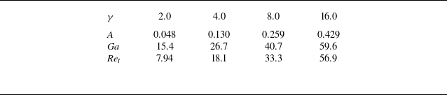
 γ
γ A=(ρ2−ρ1)/(ρ2+ρ1)
 ρ2=ρpϕb+ρf(1−ϕb)
 ρ1=ρf
ρ1=ρf Ga=(γ−1)dpgdp/ν
 Ret=|vt|dp/ν
 vt(γ)
vt(γ)
 uz(x)
uz(x) t/τt=0.02,0.10,0.17,0.25
 γ=2
γ=2

 z0
z0 z1
z1 z2
z2 ⟨ϕ⟩xy(z,t)
 t/τt
t/τt γ=2
γ=2 ⟨ϕ⟩xy
⟨ϕ⟩xy t/τt=0.25
 τ
τ τg
τg τt
τt γ=2
γ=2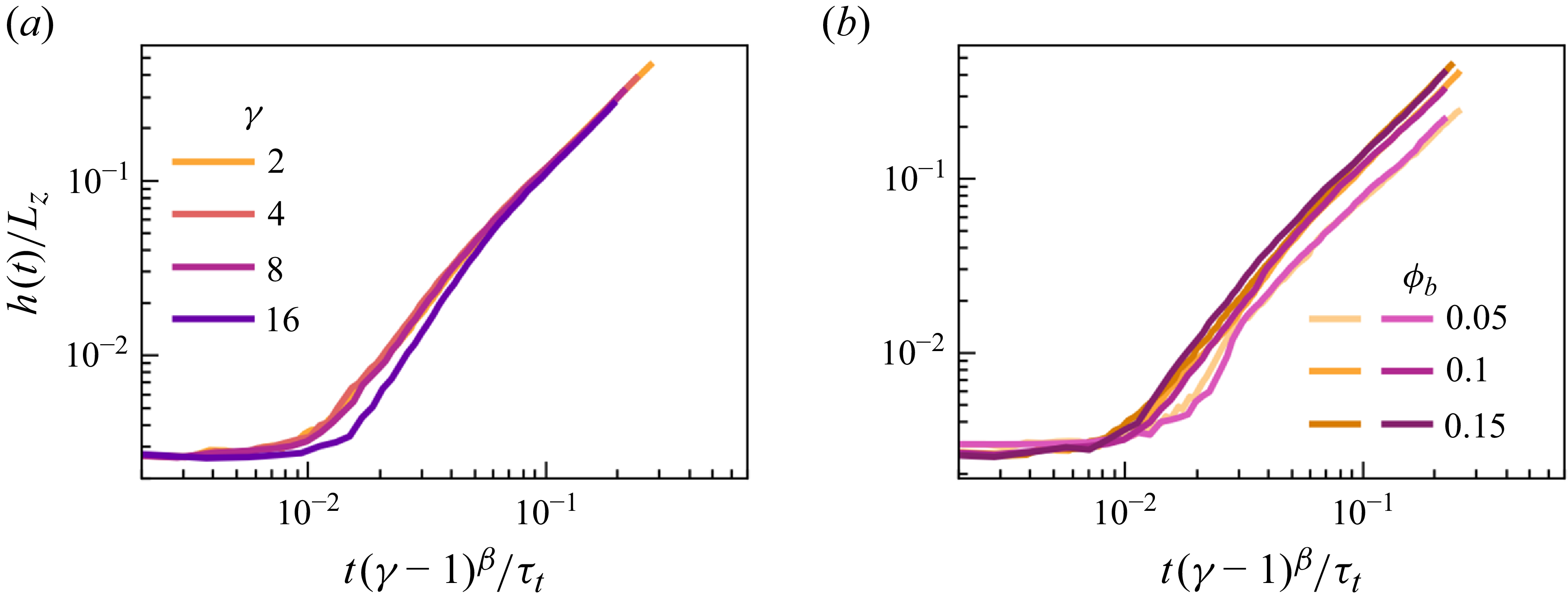
 ϕb=0.10
 γ
γ γ=2,8
γ=2,8 ϕb
ϕb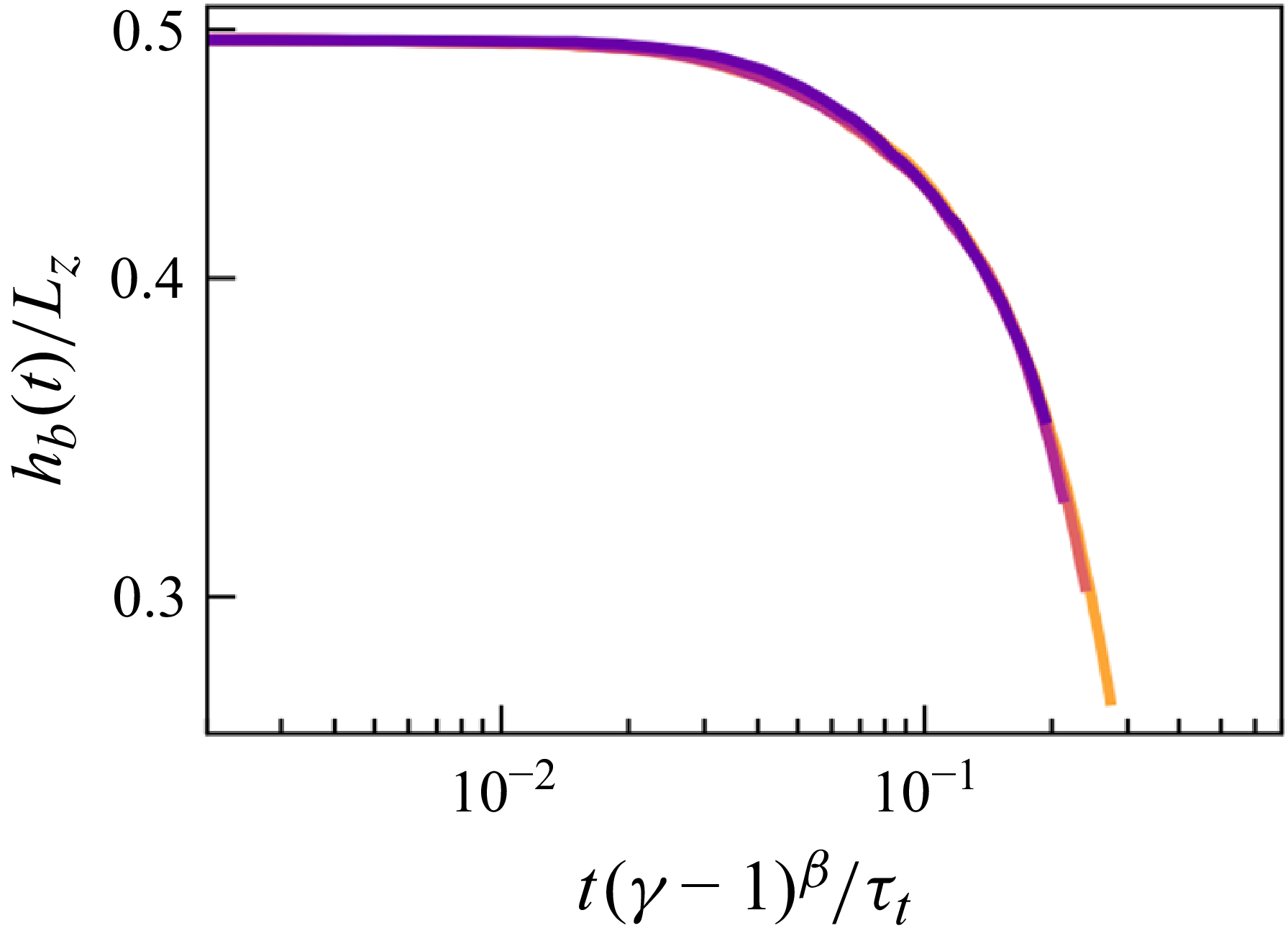
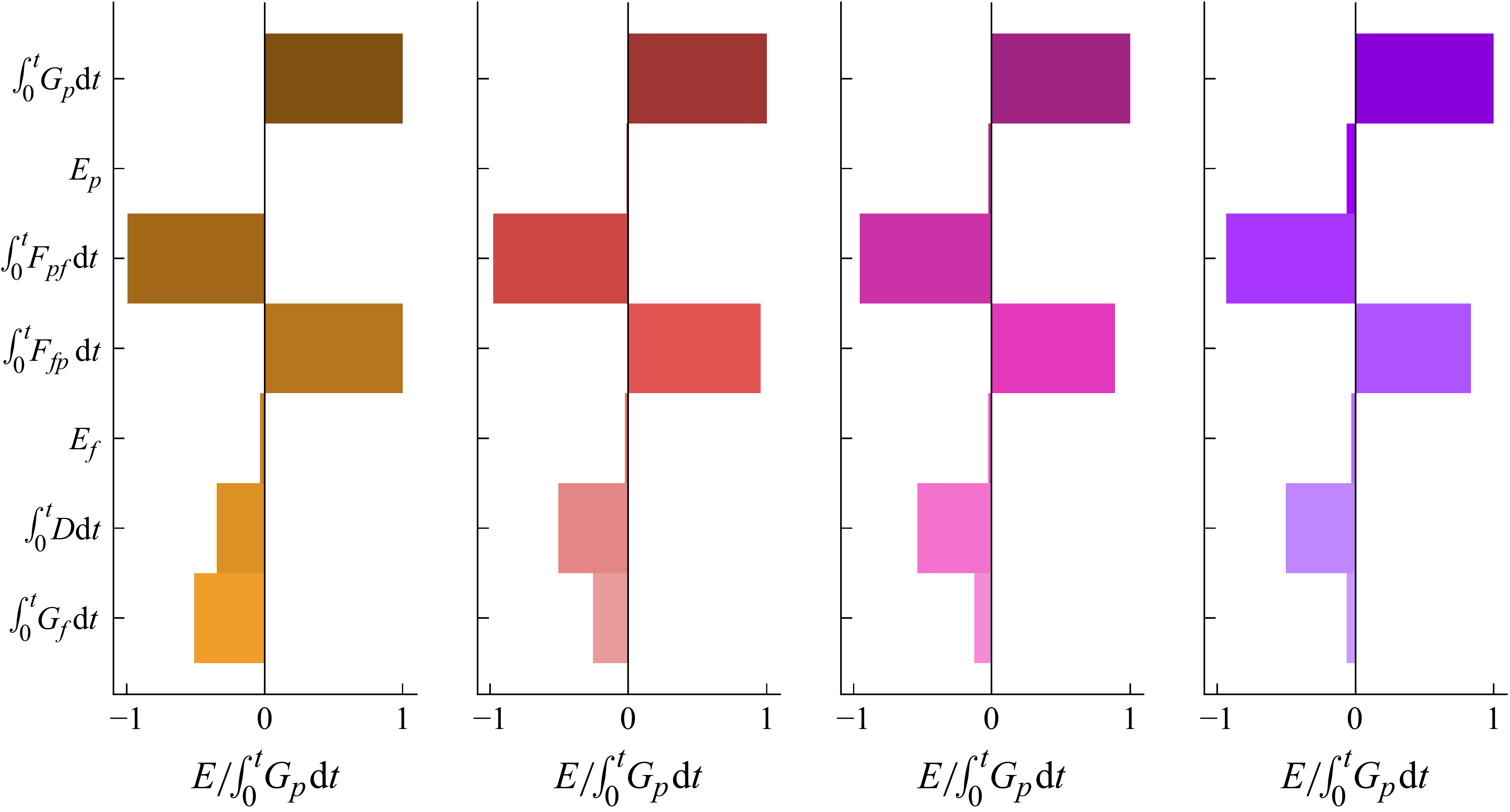
 t/τg≈0.5
 γ
γ F
F
 Δt/τt=0.0290, 0.0440, 0.0405, 0.0691
 γ=2
γ=2 16
16 t/τg≈0.5
 γ=16
γ=16 t/τt=0.69
 T
T κp=2π/dp
 Δt/τt=0.0290, 0.0440, 0.0405, 0.0691
 γ=2
γ=2 16
16 t/τg≈0.5
 κp=2π/dp
 γ
γ Ixym
Ixym ηm
ηm Ixyb
Ixyb ηb
ηb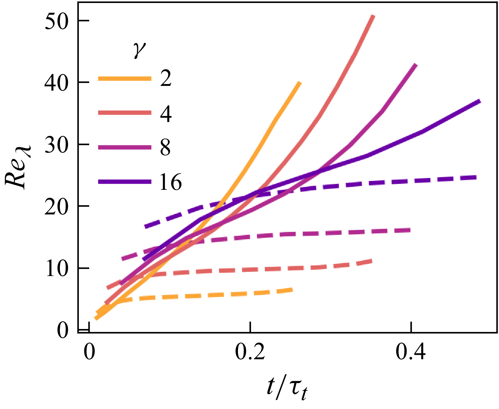
 Reλ
Reλ γ
γ Reλm
Reλm Reλb
Reλb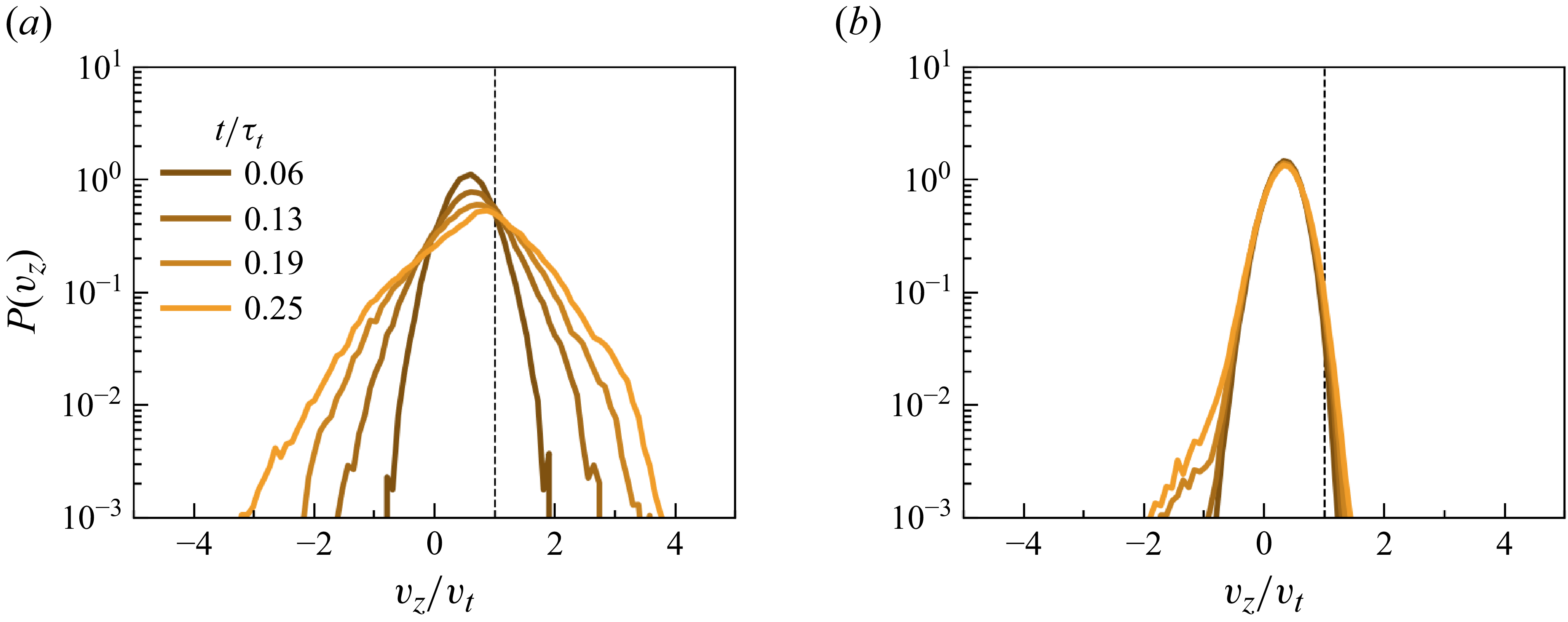
 γ=2
γ=2 vt
vt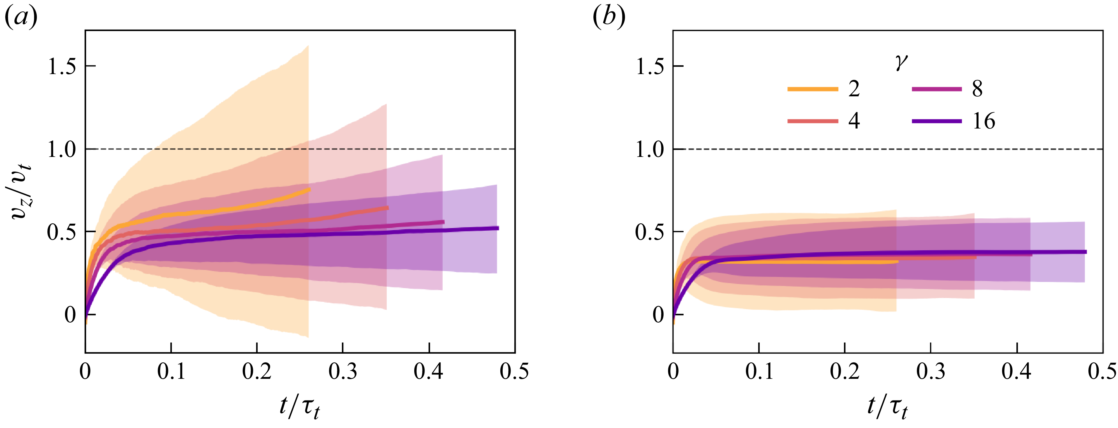
 γ
γ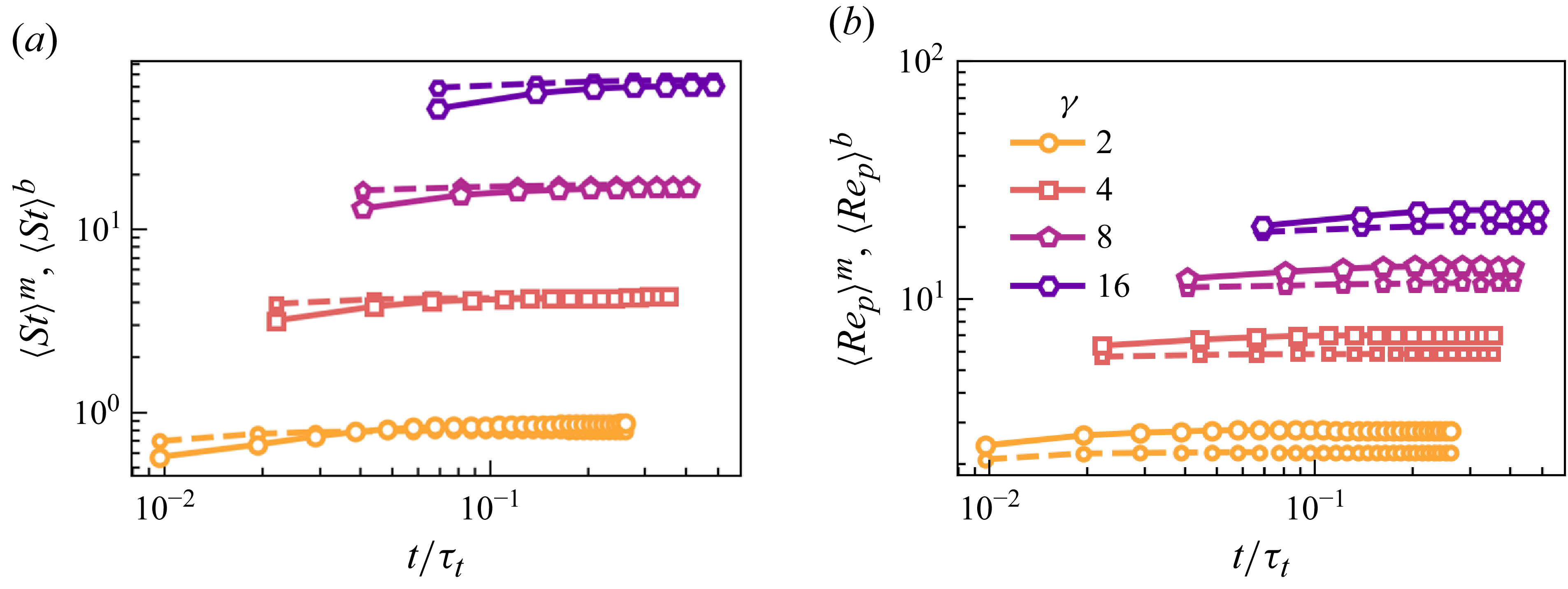
 St
St Rep
Rep
 t/τg≈0.5
 γ
γ vt
vt
 ϕ^(x)
ϕ^(x) uz(x)
uz(x) t/τg≈0.5
 ϕ^(x)
ϕ^(x)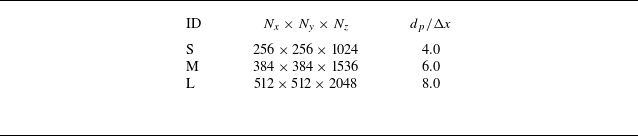
 N
N dp/Δx
dp/Δx
 t/τg≈0.5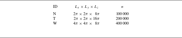
 L
L n
n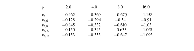
 vt
vt n
n vt,n
vt,n
 t/τg≈0.5
 Open access

