


1. Introduction
Approximately two thirds of the surface of the Earth is covered by the ocean. The air–sea exchanges of mass, momentum and energy that happen over such a vast expanse play an integral role in determining the sea state, weather patterns and climate, thus significantly impacting many aspects of human life. Although we know that surface waves need to be fully integrated into weather and global climate forecast models (e.g. Melville Reference Melville1996; Sullivan & McWilliams Reference Sullivan and McWilliams2010), we do not yet fully understand the fundamental processes that couple the surface waves with the turbulent boundary layers above and below the ocean surface (e.g. Cavaleri et al. Reference Cavaleri, Barbariol, Benetazzo and Waseda2019; Buckley, Veron & Yousefi Reference Buckley, Veron and Yousefi2020; Geva & Shemer Reference Geva and Shemer2022). Indeed, the current parameterizations of air–sea exchange processes are limited, and most models still fall short of making accurate predictions of wave growth and weather events, particularly in strongly forced conditions.
Over the past few decades, many studies have investigated the influence of ocean surface waves on air–sea exchanges and, specifically, wind stress, defined as the sum of skin friction and form drag (e.g. Banner Reference Banner1990; Belcher & Hunt Reference Belcher and Hunt1993; Melville, Shear & Veron Reference Melville, Shear and Veron1998; Sullivan, McWilliams & Moeng Reference Sullivan, McWilliams and Moeng2000; Melville, Veron & White Reference Melville, Veron and White2002; Yang & Shen Reference Yang and Shen2010; Veron, Melville & Lenain Reference Veron, Melville and Lenain2011; Grare et al. Reference Grare, Peirson, Branger, Walker, Giovanangeli and Makin2013; Grare, Lenain & Melville Reference Grare, Lenain and Melville2018; Hao & Shen Reference Hao and Shen2019; Husain et al. Reference Husain, Hara, Buckley, Yousefi, Veron and Sullivan2019; Yousefi, Veron & Buckley Reference Yousefi, Veron and Buckley2020, Reference Yousefi, Veron and Buckley2021; Aiyer, Deike & Mueller Reference Aiyer, Deike and Mueller2023, among others). These studies have shown that the drag at the ocean surface strongly depends on environmental conditions and is a function of not only wind speed but also wave height, wave slope, wind–wave alignment and wave age, which is defined as the ratio of the wave phase speed to the reference wind speed measured at a height of 10 m above the air–water interface. Although some parameterizations exist to account for the impact of these parameters on surface stress (e.g. Fairall et al. Reference Fairall, Bradley, Hare, Grachev and Edson2003; Edson et al. Reference Edson, Jampana, Weller, Bigorre, Plueddemann, Fairall, Miller, Mahrt, Vickers and Hersbach2013; Teixeira Reference Teixeira2018; Porchetta et al. Reference Porchetta, Temel, Muñoz-Esparza, Reuder, Monbaliu, Van Beeck and van Lipzig2019; Husain, Hara & Sullivan Reference Husain, Hara and Sullivan2022a,Reference Husain, Hara and Sullivanb), there is only a partial understanding of the dependencies of sea-surface drag on wave parameters. Therefore, determining these dependencies and developing sea-state-aware parametrizations of wind stress have remained one of the central foci of the wind-wave research community. Furthermore, the effects of surface waves and the corresponding generation of turbulence, airflow separation, spray and bubbles on the surface drag are not well understood. Irrespective of these findings, most operational models used to date still rely on simple bulk parameterization based on the Monin–Obukhov similarity theory (e.g. Hara & Belcher Reference Hara and Belcher2004; Hara & Sullivan Reference Hara and Sullivan2015), which is only valid under equilibrium conditions and does not account for the multiscale nature of sea-surface roughness nor the sea-state dynamics. As such, these models often struggle to accurately predict the evolution of wave fields (e.g. Moon et al. Reference Moon, Hara, Ginis, Belcher and Tolman2004b; Moon, Ginis & Hara Reference Moon, Ginis and Hara2004a; Donelan et al. Reference Donelan, Curcic, Chen and Magnusson2012; Cronin et al. Reference Cronin2019; Husain et al. Reference Husain, Hara and Sullivan2022a,Reference Husain, Hara and Sullivanb).
Accurately simulating wind-wave fields over a realistic range of the parameter space hinges upon our ability to resolve sea-surface drag. However, resolving the drag directly at the ocean surface through, for example, direct numerical simulations (DNSs) or wall-resolved large-eddy simulations (LESs) is only possible at modest Reynolds numbers due to the inherent complexity of interfacial mechanisms occurring over a broad range of time and length scales (e.g. Sullivan & McWilliams Reference Sullivan and McWilliams2010; Ayet & Chapron Reference Ayet and Chapron2022). Wall-modelled LES offers a pathway to address this challenge. In wall-modelled LES, the near-surface region is bypassed, and a wall-layer parameterization is instead used to account for subgrid-scale surface forces (Piomelli Reference Piomelli2008; Bose & Park Reference Bose and Park2018). However, difficulties associated with the acquisition of high-resolution field (or even laboratory) measurements close to the air–sea interface (e.g. Turney & Banerjee Reference Turney and Banerjee2008, Reference Turney and Banerjee2013; Sullivan et al. Reference Sullivan, Banner, Morison and Peirson2018) have limited the development of such parameterizations (see, for e.g. Yang, Meneveau & Shen Reference Yang, Meneveau and Shen2013; Aiyer et al. Reference Aiyer, Deike and Mueller2023). Limiting factors in the retrieval of direct field measurements include platform movement (e.g. Donelan, Drennan & Katsaros Reference Donelan, Drennan and Katsaros1997), limitations of existing sensor technology (e.g. Graber et al. Reference Graber, Terray, Donelan, Drennan, Van Leer and Peters2000), broadband variability of ocean wave fields (e.g. Sullivan & McWilliams Reference Sullivan and McWilliams2010) and cost. In addition, in situ observations often rely on point measurement techniques that only provide time-averaged statistics. As a result, the existing computational models and available measurement techniques are both characterized by considerable uncertainty, and findings from these two approaches are often difficult to reconcile in terms of, for example, total wind stress and wave growth (e.g. Belcher & Hunt Reference Belcher and Hunt1998; Peirson & Garcia Reference Peirson and Garcia2008; Hara & Sullivan Reference Hara and Sullivan2015).
The action of wind imparts both momentum and energy fluxes to the wave field. At the air–water interface, the total momentum flux, or the wind stress, is the sum of the tangential and form drag (e.g. Grare et al. Reference Grare, Peirson, Branger, Walker, Giovanangeli and Makin2013; Buckley et al. Reference Buckley, Veron and Yousefi2020), i.e.
 \begin{equation} \tau = \bar{\tau}_{\nu} + \bar{\tau}_{f} = \bar{\tau}_{\nu} + \overline{p \frac{\partial \eta}{\partial x}} , \end{equation}
where  $\tau _{\nu }$ is the interfacial tangential viscous stress (see § 2.1), $\tau _{f}$ is the form drag, $p$ is the pressure at the interface, $\eta$ is the surface elevation and the overbar denotes temporal or spatial averaging. Using linear spectral decomposition of the wave field, it can be further shown that the total energy input to both waves and surface currents is directly related to the wind stress
 \begin{equation} S_{in} = \overline{\tau_{\nu} u_s} + \overline{p\frac{\partial \eta}{\partial x}} c = \left( \bar{\tau}_{wc} + \bar{\tau}_f \right)c, \end{equation}
where  $u_s$ is the surface velocity, $c$ is the phase speed and ${\tau }_{wc}$ is the wave-coherent tangential stress. Consequently, the momentum flux leading to wave growth has two components, the form drag and the wave-coherent tangential stress. Knowledge of the energy input rate (or equivalently, wind stress) and its dependence on wave field characteristics is then of fundamental importance in modelling the air–sea momentum flux. Two common models for the energy input rate are developed by Jeffreys (Reference Jeffreys1925) and Miles (Reference Miles1957) from theoretical considerations and have been widely employed. These theories are, however, unable to reconcile their predictions with available field measurements.
Reconstructing the near-surface flow fields and evaluating the surface wind stress from observable, readily available free-surface characteristics, such as wave profile, wave speed and reference wind speed, are of significant interest to various geophysical and engineering applications. There is a growing appreciation of the necessity of integrating wave effects into simple one-dimensional column models of the marine boundary layers for use in climate prediction and regional ocean mesoscale codes (e.g. Donelan Reference Donelan1998; Hanley & Belcher Reference Hanley and Belcher2008; Makin Reference Makin2008). Hence, the capability to interpret the surface drag from easy-to-acquire wave features can enable reliable, real-time wave models by measuring, for example, wave heights, surface currents and sea-surface temperature using remote sensing and aerial imaging techniques (e.g. Huang et al. Reference Huang, Carrasco, Shen, Gill and Horstmann2016; Metoyer et al. Reference Metoyer, Barzegar, Bogucki, Haus and Shao2021). To that end, data-driven methods have the potential to complement field and experimental measurements and to be used as a promising tool for developing reliable surface-drag parameterizations.
Over the past few years, fluid dynamics and turbulence research has undergone a significant transformation due to the advent of machine learning (ML) techniques (e.g. Kutz Reference Kutz2017; Brenner, Eldredge & Freund Reference Brenner, Eldredge and Freund2019; Brunton, Noack & Koumoutsakos Reference Brunton, Noack and Koumoutsakos2020; Fukami, Fukagata & Taira Reference Fukami, Fukagata and Taira2020a). The ML approaches have been successfully used to accelerate computational fluid dynamics (e.g. Bar-Sinai et al. Reference Bar-Sinai, Hoyer, Hickey and Brenner2019; Kochkov et al. Reference Kochkov, Smith, Alieva, Wang, Brenner and Hoyer2021; Jeon, Lee & Kim Reference Jeon, Lee and Kim2022), develop improved turbulence closures (e.g. Ling, Kurzawski & Templeton Reference Ling, Kurzawski and Templeton2016; Wang, Wu & Xiao Reference Wang, Wu and Xiao2017; Beck, Flad & Munz Reference Beck, Flad and Munz2019; Duraisamy, Iaccarino & Xiao Reference Duraisamy, Iaccarino and Xiao2019), reconstruct turbulent flow fields from spatially limited data (e.g. Liu et al. Reference Liu, Tang, Huang and Lu2020; Fukami, Nakamura & Fukagata Reference Fukami, Nakamura and Fukagata2020b; Kim et al. Reference Kim, Kim, Won and Lee2021), predict the spatio-temporal behaviour of turbulent flows (e.g. Wang et al. Reference Wang, Kashinath, Mustafa, Albert and Yu2020; Fukami, Fukagata & Taira Reference Fukami, Fukagata and Taira2021; Zhang & Zhao Reference Zhang and Zhao2021) and advance surrogate modelling of turbulent boundary layer flows (e.g. Hora & Giometto Reference Hora and Giometto2023). However, in contrast to the flow over solid surfaces, the applications of ML approaches to air–sea interactions have been quite limited and mainly focused on predicting wave characteristics (e.g. James, Zhang & O'Donncha Reference James, Zhang and O'Donncha2018; O'Donncha et al. Reference O'Donncha, Zhang, Chen and James2018, Reference O'Donncha, Zhang, Chen and James2019; Rasp & Lerch Reference Rasp and Lerch2018; Sun et al. Reference Sun, Huang, Luo, Luo, Wright, Fu and Wang2022; Zhang et al. Reference Zhang, Zhao, Jin and Greaves2022; Dakar et al. Reference Dakar, Fernández Jaramillo, Gertman, Mayerle and Goldman2023; Lou et al. Reference Lou, Lv, Dang, Su and Li2023; Xu, Zhang & Shi Reference Xu, Zhang and Shi2023). The existing works have employed different ML frameworks to reduce the computational complexity in estimating statistical wave conditions, such as significant wave height and peak wave period, and in low-dimensional learning of wave propagation (e.g. Sorteberg et al. Reference Sorteberg, Garasto, Cantwell and Bharath2020; Alguacil et al. Reference Alguacil, Bauerheim, Jacob and Moreau2021; Deo & Jaiman Reference Deo and Jaiman2022). For instance, O'Donncha et al. (Reference O'Donncha, Zhang, Chen and James2018) integrated the SWAN (simulating waves nearshore) model into an ML algorithm to resolve wave conditions (see also James et al. Reference James, Zhang and O'Donncha2018; O'Donncha et al. Reference O'Donncha, Zhang, Chen and James2019). Further, Sun et al. (Reference Sun, Huang, Luo, Luo, Wright, Fu and Wang2022) developed a deep learning-based bias correction method for enhancing significant wave height predictions of the WW3 (Wave Watch III) model over the Northwest Pacific Ocean region (see also Campos et al. Reference Campos, Krasnopolsky, Alves and Penny2020; Ellenson et al. Reference Ellenson, Pei, Wilson, Özkan-Haller and Fern2020). These studies have demonstrated the potential of ML in predicting the propagation of surface waves and improving the predictive performance of current wave models.
The reconstruction of flow field features from surface wave characteristics is, however, more challenging and has unique complications associated with multiscale wave profiles and motions. In previous research, limited efforts have been made to reconstruct the turbulent flow above/below surface waves based only on wave observations (e.g. Smeltzer et al. Reference Smeltzer, Æsøy, Ådnøy and Ellingsen2019; Gakhar, Koseff & Ouellette Reference Gakhar, Koseff and Ouellette2020; Xuan & Shen Reference Xuan and Shen2023; Zhang et al. Reference Zhang, Hao, Santoni, Shen, Sotiropoulos and Khosronejad2023). Using convolutional neural network (CNN) classifiers, Gakhar et al. (Reference Gakhar, Koseff and Ouellette2020) demonstrated that surface elevation information alone can be used to determine the physical features at the bottom boundary (see also Mandel et al. Reference Mandel, Rosenzweig, Chung, Ouellette and Koseff2017; Gakhar, Koseff & Ouellette Reference Gakhar, Koseff and Ouellette2022). More recently, Xuan & Shen (Reference Xuan and Shen2023) explored the feasibility of using a CNN to reconstruct the turbulent flow beneath free-surface flows using the surface elevation and velocity (see also Li, Xuan & Shen Reference Li, Xuan and Shen2020). Their CNN-based model was trained on a dataset obtained from DNSs of turbulent open-channel flows over a deformable surface and could accurately reconstruct the near-surface flow field.
In the absence of accurate parameterizations of the sea-surface drag (see, for e.g. Sullivan & McWilliams Reference Sullivan and McWilliams2010; Zachry et al. Reference Zachry, Schroeder, Kennedy, Westerink, Letchford and Hope2013; Gao et al. Reference Gao, Peng, Gao and Li2020), ML-based approaches may thus offer a practical alternative. To date, however, there has been no attempt to apply such data-driven algorithms to model the sea-surface drag. In the present study, using a supervised ML framework, we aim to estimate the surface viscous stress (or skin-friction drag) of wind-generated surface waves solely from wave profiles and wave age. To that end, we develop a CNN model that takes surface elevation profiles and the corresponding wave age as inputs and predicts the spatial distribution of skin-friction drag over wind waves. The CNN network is trained using high-resolution laboratory measurements of velocity fields obtained over a range of wind-wave conditions. The experimental dataset used in the current study is based on a re-analysis of the existing raw data of Yousefi et al. (Reference Yousefi, Veron and Buckley2020). We find that, for unseen wind-wave regimes that fall within the training samples, the CNN model can accurately predict the overall distribution of instantaneous and area-aggregate viscous stresses using only the surface signatures, wave phase speed and the mean wind speed magnitude aloft. In addition, we also assess the performance of the model in capturing unseen wind-wave conditions (i.e. out-of-training distribution). To the best of the authors’ knowledge, this is the first successful attempt in the literature to model the sea-surface drag using surface signatures and wave age. The proposed CNN model can be easily tailored to serve as a wall-layer model for skin-friction contributions in wall-modelled LESs of airflow over wave fields.
The rest of the paper is organized as follows. A brief description of the experimental dataset is summarized in § 2.2. The ML model details are provided in § 2.3. In § 3, the results are presented, where we assess the performance of the model to reconstruct skin-friction drag for both the interpolation and extrapolation tasks. Further discussions on the applicability and limitations of the CNN model are offered in § 4. Finally, a brief conclusion is presented in § 5.
2. Methodology
2.1. Theory
At the air–water interface, the total wind stress is the sum of the tangential viscous stress (i.e. skin-friction drag) and the pressure stress (i.e. form drag),  $\tau ={\tau }_{\nu }+{\tau }_f$. The skin-friction drag can be estimated by
 \begin{equation} {\tau }_{\nu }=\left(\boldsymbol{\tau }\boldsymbol{n}\right)\boldsymbol{\cdot} \boldsymbol{t} , \end{equation}
where  $\boldsymbol {\tau } = \mu (\boldsymbol {\nabla }\boldsymbol {u} + \boldsymbol {\nabla }{\boldsymbol {u}}^\mathrm {T})$ is the airside viscous stress tensor estimated at the air–water interface, $\mu$ is the air dynamic viscosity, $\boldsymbol {\nabla }{\boldsymbol {u}}$ and $\boldsymbol {\nabla }{\boldsymbol {u}}^\mathrm {T}$ denote the velocity gradient tensor and its transpose, $\boldsymbol {u} = (u,w)$ are velocities in the vertical plane aligned with the direction of wave propagation and $\boldsymbol {n}$ and $\boldsymbol {t}$ are unit vectors that are, respectively, normal and tangent to the local water surface, as shown in figure 1. Considering the velocity field in the vertical plane to be aligned with the direction of wave propagation, the skin-friction drag can then be estimated by
 \begin{equation} {\tau }_{\nu } = \mu \left(\frac{\partial u}{\partial z} + \frac{\partial w}{\partial x}\right) + 2\mu \epsilon \left(\frac{\partial w}{\partial z}-\frac{\partial u}{\partial x}\right) , \end{equation}
where  $x$ and $z$ are the streamwise and vertical coordinate directions, respectively, and $\epsilon = {\partial \eta }/{\partial x}$ is the local surface slope. It should be noted here that, in (2.2), the skin-friction drag is obtained to the first order in $\epsilon$ (see Longuet-Higgins Reference Longuet-Higgins1969; Buckley et al. Reference Buckley, Veron and Yousefi2020; Yousefi & Veron Reference Yousefi and Veron2020). The form drag can also be expressed by $\tau _f = p \epsilon$. However, in the current study, we focus on skin-friction drag only.
Schematic representation of two-dimensional airflow velocity measurements obtained using the PIV technique above wind-driven surface waves. The mean flow profiles, kinematic processes and drag partitioning (into the skin-friction drag and form drag) at the air–water interface are also shown. The global coordinate system in the PIV plane is  $(x, z)$ in the streamwise and vertical directions, respectively. The surface-following coordinate system $(t, n)$ is also represented, where $\boldsymbol {t}$ and $\boldsymbol {n}$ are unit vectors that are tangent and normal to the local instantaneous water surface. At the wavy water surface, it is noted that $\epsilon = {\partial \eta }/{\partial x}$ and $\theta = \arctan {(\epsilon )}$.

2.2. Experimental dataset
In the current work, in order to train and examine the ML algorithm, we used the existing dataset of high-resolution airflow velocity measurements above wind-generated surface waves. The measurements were acquired using a combination of the particle image velocimetry (PIV) and laser-induced fluorescence (LIF) techniques in the wind-wave tunnel facility at the Air–Sea Interaction Laboratory of the University of Delaware. The facility is designed for studying atmosphere–ocean interactions, and its wave tank is approximately 42 m long, 1 m wide and 1.25 m high. The mean water level was kept at 0.7 m to allow sufficient space above the air–water surface. The tank is also equipped with a permeable wave-absorbing beach to dissipate the wave energy and prevent wave reflections. The wind tunnel of the facility can generate 10 m equivalent wind speeds of up to  $30\ {\rm m}\ {\rm s}^{-1}$. It is equipped with a honeycomb straightener to provide uniform airflow across the tank and a smooth transition from the wind tunnel inlet to the water surface. The facility, experimental set-up and image acquisition and processing procedures are described in detail in Yousefi (Reference Yousefi2020). Here, we briefly summarize the experimental set-up to put the available measurements into perspective.
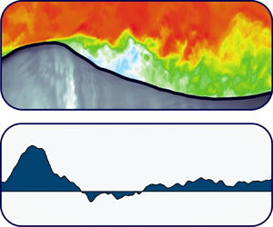
High-resolution two-dimensional velocity fields above wind waves were obtained using PIV. In combination with PIV measurements, the LIF technique was employed to precisely detect the surface profiles. This allowed the acquisition of airside velocity measurements very close to the surface within the airside viscous sublayer, as close as  $100\ \mathrm {\mu }{\rm m}$ to the air–water interface, on average. Examples of streamwise velocity measurements along the wave field are plotted in figure 1. Figure 2 also shows an example of the PIV velocity field over a separating wind wave with the corresponding skin-friction drag at the air–water interface calculated using (2.2). These experimental measurements were acquired at a fetch of 22.7 m for various wind-wave conditions with different 10 m equivalent wind speeds varying from 2.25 to $16.59\ {\rm m}\ {\rm s}^{-1}$. This resulted in purely one-dimensional waves that only propagate in the streamwise direction such that wave groups and individual waves within those groups generally align in the same direction. The wave age of the generated waves is in the range of 0.06–0.21, which corresponds to moderately to strongly forced wind waves (Drennan et al. Reference Drennan, Graber, Hauser and Quentin2003). For reference, the complete experimental conditions are listed in table 1.
An example of the instantaneous streamwise PIV velocity field over a separating wind wave (a) with the corresponding wave age, wave profile and skin-friction drag at the air–water interface (b). The objective of the CNN-based ML model is to estimate the skin-friction drag,  $\tau _{\nu }$, over wind waves from the wave profile, $\eta (x)$, and wave age, $C_p/U_{10}$. In the experimental measurements, the surface tangential viscous stress (or, equivalently, skin-friction drag) is the first value of the viscous stress measurements taken at the height of $94.8\ \mathrm {\mu }{\rm m}$ above the air–water interface.

Summary of the experimental data and wind-wave conditions. The friction and 10 m extrapolated velocities were calculated from the experimental data by fitting the logarithmic part of the mean wind velocity profile. Parameters with subscript  $p$ indicate the peak wave values obtained from peak wave frequencies by applying linear wave theory. For additional details on experimental data and procedures, the reader is referred to publications by Yousefi (Reference Yousefi2020) and Yousefi et al. (Reference Yousefi, Veron and Buckley2020).

The spectra of the generated surface wave elevations were relatively narrow banded for all experimental conditions, with peaks at the dominant wave frequency (see Yousefi et al. Reference Yousefi, Veron and Buckley2020). As reported in table 1, the dominant wave frequencies decrease with increasing wind speed because the fetch-limited waves grow longer with increasing wind speed. However, the spectral densities increase with increasing wind speed, which indicates that the waves also increase in amplitude with increasing wind speed. Under these experimental conditions, the wavelength of wind-generated surface waves varies approximately from 15 to 50 cm, which is at larger scales than capillary waves with a wavelength in the sub-centimetre range (e.g. Slavchov, Peychev & Ismail Reference Slavchov, Peychev and Ismail2021). The complications of bubble/spray generation were also largely avoided in these wind-wave conditions. Therefore, the effect of surface tension force on surface wave profiles is negligible and does not directly contribute to the viscous stress at the air–water interface.
2.2.1. Data pre-processing
The experimental dataset used to train and evaluate the ML model comprises various wind speed conditions, with each experiment sampling approximately the same number of waves. This resulted in the acquisition of more instantaneous PIV fields (which have a fixed footprint) when the wind waves were longer. Specifically, the dataset consists of approximately 2000, 3800, 4500, 4900 and 5000 instantaneous PIV images corresponding to wind speeds of  $U_{10} = 2.25$, 5.08, 9.57, 14.82 and $16.59\ {\rm m}\ {\rm s}^{-1}$, respectively. For training and validation of the ML model, we considered experiments with a wind speed of 5.08, 9.57 and $16.59\ {\rm m}\ {\rm s}^{-1}$ (corresponding to W1-05, W1-09 and W1-16 cases in table 1), resulting in a total of roughly 13 300 input–output pairs. These pairs were further randomly divided into training, validation and testing sub-datasets, where each set included 80 %, 10 % and 10 % of the total samples, respectively. The training dataset is used to train the ML model, allowing it to learn and adjust internal parameters to minimize prediction errors, while the validation subset is utilized to further fine tune the model's hyperparameters during training (e.g. Goodfellow, Bengio & Courville Reference Goodfellow, Bengio and Courville2016). Finally, in order to assess the generalization capability of the model and validate its performance in a more realistic scenario, we examined the model on out-of-training-distribution datasets. To this end, we used instantaneous PIV images of the cases with wind speeds of $U_{10} = 2.25$ and $14.82\ {\rm m}\ {\rm s}^{-1}$ as a separate dataset to examine the model performance on completely unseen data. Notably, the $U_{10} = 2.25\ {\rm m}\ {\rm s}^{-1}$ case is outside the wind speed training range.
The signal-to-noise ratio of PIV velocity measurements naturally degrades in near-surface areas due to various factors, including the reflection of high-intensity laser light off the surface and the presence of other background noise sources. Although this does not affect velocity measurements of the current experimental dataset, the interfacial skin-friction drag experiences an increased level of noise because the gradient operator introduces additional noise to the measurement. It was observed that the performance of the ML algorithm is sensitive to the near-surface noise present in the experimental data. In order to ensure the optimal performance of the ML network, a zero-phase (smoothing) infinite-impulse-response filter (e.g. Gustafsson Reference Gustafsson1996) was applied to the along-wave surface tangential stress profiles
 \begin{equation} \left.\begin{gathered} y_0[n] = \frac{1}{a_0} \left(\sum_{i=0}^{m} b_i x[n-i] - \sum_{j=1}^{m} a_j y_0[n-j]\right) \\ \mathrm{and} \\ y_1[n] = \frac{1}{a_0} \left(\sum_{i=0}^{m} b_i y_0[n+i] - \sum_{j=1}^{m} a_j y_1[n+j]\right) , \end{gathered}\right\} \end{equation}
where  $y_0[n]$ and $y_1[n]$ are, respectively, the output of forward and reverse filtering operation at location index $n$,
$n$,  $x[n]$ is the input signal, $b_i$ are the feedforward filter coefficients, $a_j$ are the feedback filter coefficients and $m$ is the filter order. An example of filtered skin-friction drag (along with other ML input data) and original experimental data are presented in figures 3(d) and 3(h) over a separating and non-separating wind wave. Further, in order to expedite the training process, we scaled the data to have zero mean and unit standard deviation. This standardization ensures that features are placed on a comparable scale, thereby facilitating more effective training of the ML model (e.g. Goodfellow et al. Reference Goodfellow, Bengio and Courville2016).
An example of ML input data over non-separating (a–d) and separating (e–h) wind waves for the wind-wave experimental condition of  $U_{10} = 5.08\ \textrm {m}\ \textrm {s}^{-1}$. The instantaneous fields of normalized streamwise velocity, $u/U_{10}$, are shown in panels (a,e), in which solid lines denote the wave profiles. The panels below each wave show (b,f) the local wave slope, $\epsilon = {\partial \eta } / {\partial x}$, (c,g) the local wave phase, $\varphi$, and (d,h) the skin-friction drag scaled with total stress, $\tau _{\nu } / \tau$, where the experimental data are indicated with cross symbols and the solid lines are the filtered experimental tangential stress profiles.

2.3. Machine learning model
The main objective of this work is to develop a model to accurately estimate the instantaneous skin-friction drag,  $\tau _{\nu }$, of surface wind waves from wave profiles, $\eta (x)$, local interface slope, $\partial \eta /\partial {x}$, local wave phases, $\varphi$, and the wave age of the corresponding wave field, $C_p/U_{10}$. In particular, we aim to develop a mapping such that
 \begin{equation} \mathcal{M}: \left( C_p/U_{10}, \eta(x), \partial\eta/\partial x, \varphi \right) \xrightarrow[]{} \tau_{\nu} (x) . \end{equation}
The CNN-based ML model is employed to approximate  $\mathcal {M}$; a detailed description of network architecture is introduced in the following section. Here, we used wave age as a dimensionless parameter incorporating wind speed rather than wave Reynolds number ( ${Re_w} = U_{10}/\nu k$ with $k$ being the wavenumber) because the wave age provides a better metric to characterize different ocean regimes (for e.g. see Csanady Reference Csanady2001; Alves, Banner & Young Reference Alves, Banner and Young2003; Sullivan & McWilliams Reference Sullivan and McWilliams2010). In addition, the Re w is indirectly incorporated into the ML model as all the parameters that define ${Re_w}$ are already included in the mapping. Although we used the wave age as a non-dimensionalized input for the ML model, the wave age only covers a small range of wind-generated surface waves in these constant fetch laboratory experiments (see table 1). Therefore, in the remainder of the paper, we will narrow our analysis to wind speed, except when wave age is a convenient parameter to compare our results with available data. It should also be noted that the Bond number ( ${BO} = {\Delta \rho g}/{\sigma k^2}$, where $\Delta \rho$ is the air–water density difference, $g$ is the gravity and $\sigma$ is the surface tension) of surface wave cases considered for this study is relatively large for all cases, varying from $BO=65$ for the lowest wind speed of $2.25\ \textrm {m}\ \textrm {s}^{-1}$ to $BO=975$ for the highest wind speed of $16.59\ \textrm {m}\ \textrm {s}^{-1}$, indicating that the surface tension effects are negligible (e.g. Van Hooft et al. Reference Van Hooft, Popinet, Van Heerwaarden, Van der Linden, De Roode and Van de Wiel2018). Hence, due to the high Bond number of wind waves, we did not include the Bond number as a mapping parameter.
2.3.1. Convolutional neural network
Neural network-based ML models, notably the multi-layer perceptron (MLP) and CNN, are widely adopted for tackling complex nonlinear regression tasks across diverse scientific and engineering domains (e.g. Rumelhart, Hinton & Williams Reference Rumelhart, Hinton and Williams1986; LeCun et al. Reference LeCun, Bottou, Bengio and Haffner1998; Goodfellow et al. Reference Goodfellow, Bengio and Courville2016). While both models are commonly used in multi-output regression tasks, MLP-based models are preferred for pointwise mapping (e.g. Raissi, Yazdani & Karniadakis Reference Raissi, Yazdani and Karniadakis2020; Maulik et al. Reference Maulik, Sharma, Patel, Lusch and Jennings2021; Hora & Giometto Reference Hora and Giometto2023), whereas CNNs excel in handling structured grid data, such as velocity fields and images (e.g. Fukami et al. Reference Fukami, Fukagata and Taira2021; Kim et al. Reference Kim, Kim, Won and Lee2021; Xuan & Shen Reference Xuan and Shen2023). This preference arises from the CNN models’ ability to capture spatially local features, exhibit translation equivariance and offer scalability advantages (see, for e.g. Goodfellow et al. Reference Goodfellow, Bengio and Courville2016; Gao, Sun & Wang Reference Gao, Sun and Wang2021). Overall, the success of CNN-based networks has established them as promising approaches for approximating complex functions.
Specifically, in the current study, we employ a CNN-based ML model (indicated by  $\mathcal {F}$) to approximate the mapping function, $\mathcal {M}$, such that
 \begin{equation} \mathcal{F} (C_p/U_{10}, \eta(x), \partial\eta/\partial x, \varphi; \boldsymbol{\mathsf{w}} ) \approx \tau_{\nu} (x) , \end{equation}
where  $\boldsymbol{\mathsf{w}}$ encompasses the trainable parameters of the CNN, including weights and biases. The CNN model used in this work primarily consists of convolutional, dense (or fully connected) and nonlinear layers. Among these, the convolutional layer plays a crucial role in capturing hierarchical representations and extracting meaningful features from the high-dimensional spatial input. This is achieved by applying the convolution operation to the input, followed by a nonlinear activation function. In a two-dimensional convolutional layer, the output ${\mathsf{h}}^{{out}}$ can be described based on the input from the previous layer, ${\mathsf{h}}^{{in}}$, as
 \begin{equation} h^{{out}}_{ijd} = \sigma \left(\sum_{k=1}^{K} \sum_{p=1}^{F} \sum_{q=1}^{F} h^{{in}}_{i+p, j+q, k} {\mathsf{w}}_{pqkd} + {\mathsf{b}}_{ijd} \right), \end{equation}
where  $\boldsymbol{\mathsf{w}}$ and $\boldsymbol{\mathsf{b}}$ denote the weight and biases of the output layer, $\sigma$ is the element-wise nonlinearity, $K$ is the number of kernels and $F \times F$ is the filter/kernel dimension (LeCun et al. Reference LeCun, Bottou, Bengio and Haffner1998; Goodfellow et al. Reference Goodfellow, Bengio and Courville2016). While convolutional layers excel at extracting local features, they have a limited receptive field and lack global awareness (e.g. Long, Shelhamer & Darrell Reference Long, Shelhamer and Darrell2015). Conversely, dense layers connect all neurons (also known as perceptrons) from the previous layer to every neuron in the current layer, enabling them to capture spatially global patterns and make predictions based on combined information from all input features (e.g. Goodfellow et al. Reference Goodfellow, Bengio and Courville2016). By incorporating dense layers towards the end of the CNN architecture, the network gains the ability to learn and encode global features. Mathematically, the transformation performed by a dense layer can be described as follows: given an input vector ${\mathsf{h}}^{in} \in {\mathsf{R}}^n$ and a weight matrix $\boldsymbol{\mathsf{w}} \in {\mathsf{R}}^{m \times n}$, the output ${\mathsf{h}}^{out} \in {\mathsf{R}}^{m}$ can be computed as
 \begin{equation} {\mathsf{h}}^{out} = \sigma \left( \boldsymbol{\mathsf{w}} {\mathsf{h}}^{in} \right). \end{equation}
The choice of an appropriate nonlinearity is crucial as it significantly impacts the training process and performance of the network for a given task (e.g. Hao et al. Reference Hao, Yizhou, Yaqin and Zhili2020). Nonlinear activation functions, including sigmoid, hyperbolic tangent (tanh) and rectified linear units (ReLU) and their variants (e.g. Nair & Hinton Reference Nair and Hinton2010; Maas et al. Reference Maas, Hannun and Ng2013; He et al. Reference He, Zhang, Ren and Sun2015), offer diverse choices to enable networks in learning complex relationships. However, gradient disappearance in sigmoid and tanh or the so-called ‘dying ReLU’ phenomenon for ReLU can adversely impact the models’ performance (e.g. Hochreiter Reference Hochreiter1998; Glorot & Bengio Reference Glorot and Bengio2010; Xu et al. Reference Xu, Wang, Chen and Li2015). Recently, Swish and Mish nonlinearity functions emerged as promising alternatives (see Ramachandran, Zoph & Le Reference Ramachandran, Zoph and Le2017; Misra Reference Misra2019), aiming to provide smoother, nonlinear behaviours, enhance the gradient flow and mitigate dead neurons. Given these properties, we employed the Mish activation, represented as  $\textrm {Mish}(x) = x \tanh [\log (1 + e^x)]$ (Misra Reference Misra2019), in the nonlinear layers of our network architecture.
Here, in order to obtain the optimal parameters  $\boldsymbol{\mathsf{w}}$ of the CNN model, we minimize the ${L}_2$ norm, also known as the mean squared error (MSE), between the ground-truth skin-friction drag obtained from experimental measurements (indicated by $\tau _{\nu }$) and the output of the ML model, $\hat {\tau }_{\nu }= \mathcal {F} (C_p/U_{10}, \eta (x), \partial \eta /\partial x, \varphi ; \boldsymbol{\mathsf{w}})$. Additionally, we incorporate ridge regularization to address the issue of overfitting. This regularization technique penalizes large values of trainable parameters, $w_i$, by augmenting the MSE loss function with the squared magnitudes of the weights. The aim is to prevent the model from assigning disproportionately large weights to specific features, a practice known to contribute to overfitting (e.g. Goodfellow et al. Reference Goodfellow, Bengio and Courville2016). In other words, our objective is to find $\boldsymbol {w}$ that minimizes the following expression:
 \begin{equation} \boldsymbol{\mathsf{w}} = \underset{\boldsymbol{\mathsf{w}}}{\arg\min} \|{ \mathcal{F}\left( C_p/U_{10}, \eta(x), \partial\eta/\partial x, \varphi; \boldsymbol{\mathsf{w}} \right) - \tau_{\nu} }\|_2 + \lambda \sum \|{ \boldsymbol{\mathsf{w}}}\|_2 , \end{equation}
where  $\lambda$ is the regularization parameter and $\sum \|{ \boldsymbol{\mathsf{w}}}\|_2$ is a ridge regularization. This optimization process enables the CNN model to learn optimal parameters, enhance performance and better approximate the underlying mapping function.
The CNN model is implemented using the Pytorch ML library (Paszke et al. Reference Paszke, Gross, Massa, Lerer, Bradbury, Chanan, Killeen, Lin, Gimelshein and Antiga2019). For  $\mathcal {F}$, based on the hyperparameter optimization analysis (see the Appendix), we adopt a CNN network with five convolutional layers, one flattened layer, one dense layer and Mish activation function for nonlinearity, as shown in figure 4. For the outputs, we employ one dense layer with a linear activation function. For all convolutional layers, the filter size is set to $F = 3$, the number of kernels is set to $K = 8$ (see (2.6)) and the number of perceptrons in a dense layer is kept at 2000. The optimal CNN-based ML model architecture is displayed in figure 4, which has 65 015 401 trainable and 0 non-trainable parameters. The network is trained end-to-end using backpropagation with the Adam optimizer (Kingma & Ba Reference Kingma and Ba2014). The Adam optimizer is an advanced stochastic gradient descent algorithm that iteratively updates the trainable parameter based on the gradients of the loss function with respect to the parameters. It incorporates adaptive learning rates and momentum, which dynamically adjust the step sizes during optimization, making the training process more efficient Kingma & Ba (Reference Kingma and Ba2014). All trainable parameters are initialized randomly using values sampled from a uniform distribution, following the approach of Glorot & Bengio (Reference Glorot and Bengio2010), and the value of regularization parameter $\lambda$ is set to $10^{-4}$. The reduce learning rate on plateau schedule is used, initializing the learning rate to $5 \times 10^{-4}$ and the rate is reduced by a factor of 0.9 when the validation loss stagnates during the training and the effective mini-batch size is set to 64.
Diagram illustrating the CNN network architecture utilized to estimate the skin-friction drag,  $\tau _{\nu }$, from $\eta (x)$, $\partial \eta /\partial {x}$, $\varphi$ and $C_p/U_{10}$. The network comprises five convolution layers (labelled ‘Conv Layers’), a flattened layer, a dense layer and the Mish activation function as the nonlinear layer. The network takes inputs including a stack of $\eta (x)$, $\partial \eta /\partial {x}$, $\varphi$ and $C_p/U_{10}$ (shown on the left), and the output $\hat {\tau }_{\nu }$ (shown on the right). Each convolutional layer employs a filter size of $F=3$ and $K=8$ filters, the dense layer contains 2000 perceptrons/neurons. The tuple (4, 8, 985) represents the number of inputs, number of kernels and number of data points, respectively.

3. Results
In this section, we evaluate the performance of the CNN model by comparing the predicted skin-friction drags against the corresponding reference high-resolution PIV measurements from the test dataset mentioned in § 2.2.1. To this end, we first analyse the convergence history of the model and present a quantitative analysis of ML-specific error metrics. We then focus on model performance based on instantaneous and averaged skin-friction fields and assess its predictive ability in estimating the viscous drag from datasets in and out of the training range.
3.1. Convergence history
In this section, we provide an overview of the ML model training process. To ensure optimal performance, careful consideration must be given to the training process, including the number of epochs or iterations. Training for an insufficient number of epochs might lead to an underfitting issue, where the model fails to capture the underlying patterns in the data. Conversely, excessive training may lead to overfitting, a phenomenon in which the model memorizes the training data and learns the present noise, losing its ability to generalize to unseen data. Balancing the trade-off between underfitting and overfitting is critical to enhance the model's performance on new, unseen data. Such a balance can be generally achieved through various methods such as cross-validation, early stopping and regularization. Incorporating these techniques, combined with the careful selection of hyperparameters and the choice of appropriate model architecture, can significantly improve the generalization performance of the regression model (e.g. Hastie, Tibshirani & Friedman Reference Hastie, Friedman and Tibshirani2009; Goodfellow et al. Reference Goodfellow, Bengio and Courville2016).
Figure 5 shows the MSE convergence history of the ML model against the number of epochs on both training and validation datasets. It is plotted on a logarithmic vertical scale to better visualize the slight differences between training and validation losses. The figure clearly illustrates a progressive decrease in MSE for both datasets as the training progresses. This indicates that the model is continuously learning and improving its accuracy. Here, to address the challenge of overfitting and enhance generalization, we employed the early stopping technique proposed by Amari et al. (Reference Amari, Murata, Muller, Finke and Yang1997) and used in existing ML-based studies (e.g. Fukami, Fukagata & Taira Reference Fukami, Fukagata and Taira2019; Srinivasan et al. Reference Srinivasan, Guastoni, Azizpour, Schlatter and Vinuesa2019; Fukami et al. Reference Fukami, Fukagata and Taira2021). Early stopping is a technique that continuously monitors the model's performance on a separate validation dataset and terminates the training process if the validation loss fails to improve or consistently deteriorates over a predefined number of epochs (five in our case). In the current work, while the training set was used to update the model parameters, the validation set was used to continuously monitor the model performance on a separate unseen dataset and prevent overfitting the training data. After approximately 150 epochs, the validation loss stopped improving, and the early stopping mechanism terminated the training. This approach allowed us to identify the optimal stopping point during training and capture a model that strikes a balance between fitting the training data and generalizing it to unseen data. At the completion of the training, the MSE values for the training and validation datasets were 0.0146 and 0.0148, respectively. The close MSE value on training and validation datasets demonstrates the model's ability to accurately learn the underlying concept, while effectively avoiding overfitting or underfitting issues.
Convergence of the MSE loss of the CNN-based ML during the training phase. Training and validation losses represent the MSE on the training and validation datasets, respectively. Epochs indicate the number of iterations used in the learning process. The vertical axis is plotted on logarithmic access to better demonstrate the slight differences between loss curves.

3.2. Model performance on the test dataset
3.2.1. Error analysis
To quantify and evaluate the performance of the CNN-based ML method, we calculate the relative mean absolute error (RMAE) and the relative mean square error (RMSE) defined based on the  ${L^1}$-norm and ${L^2}$-norm, respectively. The relative mean error can be defined by
 \begin{equation} \delta_{e, p} = \frac{\|{\tau_{\nu} - \hat{\tau}_{\nu}}\|_{p}}{\|{\tau_{\nu}}\|_{p}} , \end{equation}
where  $\hat {\tau }_{\nu }$ is the ML-predicted viscous stress, $\tau _{\nu }$ is the corresponding ground-truth experimental measurement and $\|{\cdots }\|_{p}$ is the ${L_p}$-norm defined for the vector $\boldsymbol {v}$ of size $n$ by
 \begin{equation} \|{\boldsymbol{v}}\|_{p} = {\left( \sum_{i=1}^{n} {\left| v_i \right|}^p \right)}^{{1}/{p}} . \end{equation}
Here,  $|\cdots |$ represents the absolute operator, $p=1$ indicates the RMAE and $p=2$ denotes the RMSE. Both metrics are thus a measure of the mean relative error between the ML prediction and the experimental output of skin-friction drag for each instantaneous wave. For evaluating the performance of the ML model, it is important to consider different types of errors. For completeness, we also calculated the coefficient of determination, denoted as $R^2$
$R^2$
 \begin{equation} R^2 = 1 - \frac{\sum\left(\tau_{\nu} - \hat{\tau}_{\nu} \right)^2}{\sum\left(\tau_\nu - \bar{\tau}_\nu \right)^2} , \end{equation}
where  $\bar {\tau }_\nu$ is the ensemble average of the ground-truth skin-friction drag. Here, it is noted that the performance evaluation is based on the test dataset of the corresponding wind-wave case, i.e. the ensemble averaging in (3.3) is conducted on the snapshots in the test dataset only.
The values of the  $\delta _{e,1}$, $\delta _{e,2}$ and $R^2$ metrics are reported in table 2 for all wind-wave cases. In an average sense, these values comprehensively evaluate the ML-model predictions compared with the reference experimental data. In cases for which the model has been trained, the relative errors are slightly lower, except for the highest wind speed case; in the percentage sense, the RMAE error for the W1-05, W1-09 and W1-16 cases corresponding to wind waves with $U_{10} = 5.08$, 9.57 and $16.59\ \textrm {m}\ \textrm {s}^{-1}$ are 24.0 %, 21.7 % and 34.4 %, respectively. The increase in the error metrics for the highest wind speed case compared with the moderate cases ( $U_{10} = 5.08$ and $9.57\ \textrm {m}\ \textrm {s}^{-1}$) is, in part, due to capturing only a portion of the wave profiles and the corresponding surface stresses at high wind speeds. Because of longer waves, in the two high wind speed cases of 14.82 and $16.59\ \textrm {m}\ \textrm {s}^{-1}$, there exist a number of waves for which the entire wavelength of the wave cannot be captured in the PIV field of view. We observed that the ML model performs best for the cases where at least one wavelength has been captured. Another contributor to this increased error might be the increase in the signal-to-noise ratio of the PIV measurements with wind speed. The unseen cases of W1-02 and W1-14 are discussed in § 3.4.
Summary of the ML model performance in predicting skin-friction drag compared with the experimental data. The RMAE, RMSE and coefficient of determination ( $R^2$) metrics are presented for all wind-wave conditions. Also, the W1-02 and W1-14 cases are separate datasets for which the model has been applied to examine the model interpolation and extrapolation performance on unseen data.

The relative errors reported in table 2 provide an average measure over the entire dataset. To further evaluate error distributions across individual waves and gain insights into the model accuracy on a wave-by-wave basis, we estimate the relative error for each wave. The probability density functions (p.d.f.s) of relative mean absolute and  $R^2$ errors are respectively shown in figures 6(a) and 6(b) for the W1-05, W1-09 and W1-16 cases. As is shown, the p.d.f. plots indicate that the ML model performs similarly for the W1-05 and W1-09 cases with moderate wind speeds of 5.08 and $9.57\ \textrm {m}\ \textrm {s}^{-1}$. In these cases, the most probable relative error is roughly 20 % with a coefficient of determination of approximately 0.96, where the maximum RMAE is $\max {(\delta _{e, 1})} \approx 55\,\%$ and the minimum $R^2$ is $\min {(R^2)} \approx 0.7$. The p.d.f.s of these cases also exhibit overlapping tails with small $p(\delta _{e, 1})$ values, suggesting that the probability of extreme errors ( $\mathrm {RMAE} \geqslant 40\,\%$ and $R^2 \leqslant 0.75$) is negligible. For the strongly forced wind waves (i.e. W1-16 case), however, the performance of the ML model slightly degrades, yielding a most probable relative error of $\delta _{e, 1} \approx 30\,\%$ with a coefficient of determination of $R^2 \approx 0.9$. In this case, although the maximum relative error increases to 90 %, $R^2$ remains acceptable at around 0.55.
The p.d.f.s of (a) RMAE,  $\delta _{e, 1}$, and (b) coefficient of determination error, $R^2$, for the W1-05, W1-09 and W1-16 cases with a wind speed of $U_{10}= 5.08$, 9.57 and $16.59\ \textrm {m}\ \textrm {s}^{-1}$, respectively. The RMAE and $R^2$ error metrics were calculated for each instantaneous wave in the test dataset, and their distribution of probabilities is shown here.

The decrease in the model accuracy with increasing wind speed can be attributed to more frequent airflow separation events over wind waves and the increased signal-to-noise ratio in the experimental measurements. We discuss this in more detail in § 4. Here, it should also be noted that, although the relative error may be higher in high wind speed cases, the  $R^2$ metric still demonstrates an acceptable correlation between the ML predicted and experimental values of the skin-friction drag for all wind-wave conditions. In fact, the RMAE is an average measure relative to the ground-truth experimental values. A large RMAE thus suggests that the ML model may have a large average deviation from the average magnitude of experimental values. However, the $R^2$ represents how accurately the ML predictions of surface stress can capture the variability of the corresponding experimental measurements about their respective means. This indicates that our ML model, even in cases with a high RMAE, can sufficiently explain the overall variance of the measurements as the $R^2$ values are acceptable. Although RMAE and $R^2$ are widely accepted metrics for evaluating ML model performance, their lack of physical significance may lead to misplaced confidence in the model's performance from a physical standpoint (e.g. Wang et al. Reference Wang, Kashinath, Mustafa, Albert and Yu2020; Hora & Giometto Reference Hora and Giometto2023).
3.2.2. Wave-phase-dependent errors
Here, we turn our attention to examining the accuracy of the ML model in predicting the wave-phase-dependent distribution of skin-friction drag over surface waves. The stress distributions over waves are largely wave-phase dependent, and accurate predictions of stress distributions are of significant importance for numerical simulations such as wall-modelled LESs and developing sea-state-dependent modelling frameworks. In order to analyse the behaviour of organized wave motions in a turbulent boundary layer flow, an instantaneous flow field variable may be separated into a phase-averaged (or wave-phase-dependent) component,  $\langle\, f(\boldsymbol {x}, t) \rangle$, and a turbulent fluctuation component, $f^\prime (\boldsymbol {x}, t)$, such that (Hussain & Reynolds Reference Hussain and Reynolds1970)
 \begin{equation} f(\boldsymbol{x}, t) = \langle\, f(\boldsymbol{x}, t) \rangle + f^\prime (\boldsymbol{x}, t) , \end{equation}
where  $\boldsymbol {x}$ is the position vector at time $t$. The phase-averaged quantity can be further decomposed into the sum of an ensemble mean component, $\bar {f} (\boldsymbol {x})$, and a wave-coherent component, $\tilde {f}(\boldsymbol {x}, t)$, i.e. $\langle\, f(\boldsymbol {x}, t) \rangle = \bar {f} (\boldsymbol {x}) + \tilde {f}(\boldsymbol {x}, t)$, which is defined as
 \begin{equation} \langle\, f(\boldsymbol{x}, t) \rangle = \mathop{\mathrm{lim}}\limits_{N\to \infty } \frac{1}{N}\sum^N_{n=1}{f\left(\boldsymbol{x} + n \lambda, t \right)} , \end{equation}
where  $N$ is the number of instantaneous realizations and $\lambda$ is the local wavelength. In fact, a phase-average quantity is the average of the values of that quantity at a particular phase of the wave, while the ensemble average (or equivalently, mean) is defined as the average of the quantity over all possible phases. The properties of the ensemble- and phase-averaged operators are discussed in reports by Hussain & Reynolds (Reference Hussain and Reynolds1970, Reference Hussain and Reynolds1972) and Reynolds & Hussain (Reference Reynolds and Hussain1972). The phase-averaged relative errors and r-squared distributions across wave phases are presented for W1-05, W1-09 and W1-16 experimental conditions in figures 7(a) and 7(b), respectively. It is noted that, in the current work, the local instantaneous wave phases were estimated using a Hilbert transform technique (for details, see Melville Reference Melville1983; Hristov, Friehe & Miller Reference Hristov, Friehe and Miller1998) applied to the wave profiles obtained from laboratory measurements (see Yousefi et al. Reference Yousefi, Veron and Buckley2020). In order to estimate the phase-averaged quantities, the wave phases were segregated into 108 independent bins, each covering a phase interval of $5.82 \times 10^{-2}$ rad. From figure 7, it is evident that the relative errors for moderate wind speed cases of W1-05 and W1-09 exhibit similar patterns in that both RMAE and $R^2$ have their optimum values near the wave crest, and they slightly degrade in the leeward side of the waves where the airflow separation events occur. However, although the general performance degrades for the W1-16 case, the ML model accuracy improves in the wake regions downwind of waves. The phase-averaged error metrics, in general, align with the mean values reported in table 2 and figure 6.
Phase-averaged (a) RMAE,  $\delta _{e,1}$, and (c) coefficient of determination error, $R^2$, for W1-05, W1-09 and W1-16 cases with a wind speed of 5.08, 9.57 and $16.59\ \textrm {m}\ \textrm {s}^{-1}$, respectively. The RMAE and $R^2$ metrics were calculated for each instantaneous wave in the test dataset and bin averaged based on the corresponding wave phases. The wave phases were segregated into 108 independent bins such that each bin covers a phase interval of $5.82 \times 10^{-2}$ rad. A sketch of the mean wave profile is also shown in panels (b,d) to better visualize the wave phases.

Finally, the phase-averaged predictions of the skin-friction drag,  $\langle \hat {\tau }_\nu \rangle$, are shown and compared with the corresponding experimental measurements in figure 8(a) for the wind speed of $5.08\ \textrm {m}\ \textrm {s}^{-1}$. Here, all stress profiles are normalized by the total wind stress, i.e. $\tau = \rho u^2_*$. The ML predictions of the phase-averaged viscous stress particularly show an excellent agreement with the experimental measurements. The phase-averaged distributions of viscous stress present a pattern of along-wave asymmetry in which the stress is highest upwind of the wave crest with its peak value about the crest and a minimum in the middle of the leeward side of the wave. The ML model accurately captures this behaviour. An important observation here is that the RMAE and $R^2$ calculated from the phase-averaged (and, as we see later, the ensemble-averaged) skin-friction drags demonstrate remarkable performance, indicating accurate predictions of the stress profiles in the average sense. This is because the differences between the ML predictions and experiments observed in instantaneous waves will be averaged out once all profiles are averaged into each phase bin. In the case of the W1-05 experiment, the relative error and $r$-squared are 3.1 % and 0.998, respectively. For brevity, the other cases with $U_{10} = 9.57$ and $16.59\ \textrm {m}\ \textrm {s}^{-1}$ have not been shown here. However, their relative error between the phase-averaged ML predictions and laboratory measurements of the skin-friction drag is 5.3 % and 13.9 %, respectively, with the corresponding $R^2$ values of 0.996 and 0.975. We observe the same order of accuracy of the model in predicting the ensemble-averaged viscous stresses in § 3.4.
(a) The ML predictions of the phase-averaged distributions of the normalized skin-friction drag,  $\langle \tau _{\nu } \rangle / \tau$, compared with the experimental measurements for the wind-wave condition with a wind speed of $5.08\ \textrm {m}\ \textrm {s}^{-1}$. For comparison purposes, both raw and filtered experimental data are plotted. All stress profiles are scaled using the total wind stress, $\tau = \rho u_*^2$. A sketch of the mean wave profile is also plotted in panel (b) to better visualize the wave phases. In panel (c), the p.d.f. of $\langle \tau _{\nu } \rangle / \tau$ estimated by the ML model and experimental measurements is plotted for the same of W1-05. The p.d.f. plot indicates the ability of the model to accurately predict the phase-dependent spatial distributions of skin-friction drag.

To examine the effectiveness of the proposed model in reconstructing the spatial variability of phase-averaged skin-friction drags, the p.d.f. of normalized  $\langle \tau _\nu \rangle$ for both ML predictions and empirical measurements is depicted in figure 8(c) for the W1-05 case with a wind speed of $5.08\ \textrm {m}\ \textrm {s}^{-1}$. As illustrated, the p.d.f. plots of the reconstructed viscous stress align remarkably with those derived from the experimental data, particularly for the case of moderately forced wind waves. This agreement is also observed for other cases, including the high wind speed cases (not shown here for brevity). These findings underscore the model's adeptness in predicting and reconstructing phase-averaged skin-friction drags with precise spatial distributions. Such a quantity is particularly relevant for numerical simulations based on the wall-layer modelling approach (see Piomelli Reference Piomelli2008), where the wavy surface is either known but unresolved or known and partially resolved (see, for e.g. Husain et al. Reference Husain, Hara, Buckley, Yousefi, Veron and Sullivan2019; Deskos et al. Reference Deskos, Lee, Draxl and Sprague2021).
3.2.3. Instantaneous stress reconstructions
The preceding analysis, while illustrative of the model's proficiency in reconstructing the spatial variability of phase-averaged skin-friction drags, does not facilitate a comprehensive evaluation of its ability to reconstruct local stress distributions or capture the complex dynamics of near-surface physical processes. Consequently, a more nuanced examination is required to fully elucidate these attributes. In this section, we broaden our investigation to more precisely assess the performance of the model in reconstructing the instantaneous along-wave distributions of surface viscous stress and its ability to capture the effects of near-surface separation on the skin-friction drag. Figure 9 shows the predicted instantaneous normalized skin-friction drags,  $\hat {\tau }_\nu / \tau$, for surface wave cases with a wind speed of $5.08\ \textrm {m}\ \textrm {s}^{-1}$ (a–c), $9.57\ \textrm {m}\ \textrm {s}^{-1}$ (d–f) and $16.59\ \textrm {m}\ \textrm {s}^{-1}$ (g–i) along with their corresponding experimental data for comparison. The stress profiles are all scaled by the total stress. For reference, the instantaneous streamwise velocity fields are also plotted on the top panel. Figure 9 illustrates the instantaneous spatial distributions of the tangential stress, successfully reconstructed by the ML model. This reconstruction exhibits significant alignment with the experimental reference data, even though there are minor discrepancies in the peak magnitudes. The model is particularly effective in accurately predicting airflow separation events, reflecting its robust performance in this area.
Spatial distributions of the instantaneous normalized skin-friction drag (b,e,h) obtained from experimental measurements and (c,f,i) reconstructed by the ML model over wind waves for the wind-wave experimental conditions of W1-05 (a–c), W1-09 (d–f) and W1-16 (g–i) with corresponding wind speeds of 5.08, 9.57 and  $16.59\ \textrm {m}\ \textrm {s}^{-1}$. The stress profiles are all scaled by the total wind stress. (a,d,g) Normalized instantaneous streamwise velocity fields, $u/U_{10}$, are plotted on the top panels for reference. The ML model accurately predicts significant flow features, for instance, airflow separation on the leeward side of the wave.

In the context of airflow separation, we define this phenomenon as occurring when the near-surface, high-shear layer, typically indicative of an attached boundary layer, is propelled away from the surface, causing the surface tangential stress to reduce to a near-zero value within the sheltered region. Over wind waves, the behaviour is distinctly illustrated in figure 9. Here, the skin-friction drag reaches its peak value on the windward side of the wave, but the occurrence of airflow separation triggers a considerable drop in surface stress at the separation point. Subsequently, the stress is significantly reduced, approaching zero (or even becoming negative) on the leeward side, maintaining this minimal value within the separated region. Figure 9 also demonstrates that the contribution of viscous stress to total stress diminishes with increasing wind speed. These features, which are of paramount importance from a dynamic perspective, pose formidable challenges when it comes to accurate measurement in either laboratory environments or full-scale field settings, as well as reproduction through physics-based numerical simulations. Despite these challenges, the proposed ML model has demonstrated its proficiency by reconstructing the surface viscous stress over strongly forced wind waves – waves that are subject to frequent and intermittent airflow separations.
In order to provide context for the error distributions observed in the instantaneous stress profiles, we now focus on model predictions classified into three error thresholds: low, moderate and high. These are compared against the reference experimental data for the W1-05 dataset with  $U_{10} = 5.08\ \textrm {m}\ \textrm {s}^{-1}$. Figure 10 presents the comparison between the ML-reconstructed and experimental measurements of the instantaneous along-wave skin-friction drags. Specifically, the errors are partitioned into three categories:
(i) low-level error with $\delta _{e, 1} \approx 10\,\%$ and $R^2 \approx 0.99$ (left-hand column);
(ii) moderate-level error with
$\delta _{e, 1} \approx 25\,\%$ and $R^2 \approx 0.93$ (middle column); and(iii) high-level error with
$\delta _{e, 1} \approx 65\,\%$ and $R^2 \approx 0.65$ (right-hand column).


All profiles are normalized by the total stress, and the corresponding instantaneous horizontal velocity fields are shown in figure 10(a,e,i) for reference. Even when considering higher error thresholds, as illustrated in figure 10(i–l), the model maintains acceptable accuracy in mapping the general spatial pattern of the surface viscous stress, though slight deviations are detected.
Spatial distributions of instantaneous normalized skin-friction drag obtained using (b,f,j) experimental measurements,  $\tau _\nu / \tau$ and (c,g,k) ML model predictions, $\hat {\tau }_\nu / \tau$, for the W1-05 case with $U_{10}= 5.08\ \textrm {m}\ \textrm {s}^{-1}$ at different error levels of $\delta _{e, 1} \approx 10\,\%$ and $R^2 \approx 0.99$ (a–d), $\delta _{e, 1} \approx 25\,\%$ and $R^2 \approx 0.93$ (e–h) and $\delta _{e, 1} \approx 65\,\%$ and $R^2 \approx 0.65$ (i–l). Here, all profiles are normalized by the total stress, $\tau = \rho u_*^2$, and for reference, the instantaneous horizontal velocity fields are plotted in the top panels (a,e,i). In panels (d,h,l), ML reconstructed and experimental measurements of along-wave viscous stress profiles are also compared. Even for predictions with higher error thresholds, the model accurately captures the overall trend of the along-wave surface viscous stress distribution.

For the separating wind wave under study, the model provides an adequately accurate prediction of the airflow separation event. At the separation point, the prominent viscous stress downwind of the wave crest drops to a minimal value and remains a minor portion of the total stress within the separation bubble. However, the model falls short of replicating a particular phenomenon observed in the experimental data, where the ejection of low-velocity fluid from the water surface on the windward side of the wave crest induces a subtle reduction in surface stress. Overall, the ML model does not fully succeed in encapsulating the influence of such a bursting process on surface stress, a shortfall most pronounced in scenarios involving high wind speeds. For more information on the bursting process over surface waves, readers are directed to works such as Kawamura & Toba (Reference Kawamura and Toba1988) and Yang & Shen (Reference Yang and Shen2010). Importantly, the proposed examination of instantaneous stress profiles across varying error thresholds highlights that the previous analysis, which depended solely on relative error metrics, conceals some of the essential competencies of the ML model. This realization underscores the necessity for a more sophisticated and nuanced evaluation of ML models, tailored to the specific challenges and requirements of the problem at hand.
3.3. Model generalizations
In this section, we assess the ability of the ML model to predict the local skin-friction drag under wind-wave conditions beyond those used for training and validation. To this end, a comprehensive evaluation of the model's performance in both interpolation, where training and test inputs originate from the same distribution, and extrapolation, where test inputs represent out-of-distribution instances, is essential. This dual analysis forms the cornerstone of the ML model's generalization capabilities, in line with the principles outlined, for example, in Silverman (Reference Silverman1986) and Barnard & Wessels (Reference Barnard and Wessels1992). To evaluate the model's interpolation abilities, we examine its performance using the W1-14 case with a wind speed of  $U_{10} = 14.82\ \textrm {m}\ \textrm {s}^{-1}$. This case corresponds to strongly forced wind waves and falls within the range of wind-wave conditions utilized during training. Furthermore, we explore the model's extrapolation capabilities by evaluating its performance on the low wind speed case of W1-02 with a wind speed of $U_{10} = 2.25\ \textrm {m}\ \textrm {s}^{-1}$.
In particular, the lowest wind speed case represents an entirely different wind-wave regime in which nascent short surface waves emerge and almost no waves (less than approximately 1 %) undergo airflow separation downwind of wave crests. However, in other cases, airflow separation occurs over a significant portion of waves; for example, in high wind speed cases of  $U_{10} = 14.82$ and $16.59\ \textrm {m}\ \textrm {s}^{-1}$, airflow separation occurs over nearly 90 % of waves (see Buckley et al. Reference Buckley, Veron and Yousefi2020; Yousefi Reference Yousefi2020). Although the assessment of the model using unseen datasets within and out-of-distribution ranges of wind speeds used for the model training reinforces confidence in the model's adaptability, it is important to note that these unseen datasets still cover wind-generated wave regimes. Additionally, these cases consist of experimental conditions in which wind and waves are in the same direction. Due to the limitations of the experimental dataset, we were thus unable to consider the effects of wind-wave misalignment, mechanical swells and a more complex sea that involves the combination of wind waves and swells.
The error metrics shown in table 2 shed light on the model's performance in predicting wind-wave conditions for the considered wind speeds of  $14.82\ \textrm {m}\ \textrm {s}^{-1}$ (W1-14 case) and $2.25\ \textrm {m}\ \textrm {s}^{-1}$ (W1-02 case). The relative mean errors are found to be 31.9 % and 34.2 %, respectively, coupled with corresponding $R^2$ values of 0.866 and 0.836. In the averaged sense, the model interpolation and extrapolation predictions show a degree of accuracy mirroring the estimations for surface stress in the wind-wave conditions that formed the training set. For the W1-14 case, the RMAE and $R^2$ values of the ML-model predictions display a marginal improvement compared with the W1-16 case, which features a higher $U_{10}$ value. Focusing on the low wind speed scenario where $U_{10} = 2.25\ \textrm {m}\ \textrm {s}^{-1}$, a slight decline in model performance is observable. This reduction in efficacy is attributed to the distinct nature of the low wind speed case, predominantly comprising short gravity waves with rare occurrences of airflow separation. Such a scenario contrasts with the conditions in which the model excels, particularly over separating wind waves. This behaviour underlines the importance of a comprehensive understanding of the model's behaviour across varied wind-wave scenarios and sets the stage for future refinements to enhance its general applicability and accuracy.
Further, RMAE and  $R^2$ error metrics are calculated for individual wave profiles, and their corresponding p.d.f.s are shown in figures 11(a) and 11(b), respectively, for wind-wave cases with $U_{10} = 2.25$ and $14.82\ \textrm {m}\ \textrm {s}^{-1}$. Probability density functions, therefore, evaluate the distribution of various error levels across individual waves. The peaks in the p.d.f. distributions represent the most probable RMAE and $R^2$ metrics in the dataset, which are $\delta _{e, 1} \approx 33\,\%$ and $R^2 \approx 0.87$ for the case of W1-02 and $\delta _{e, 1} \approx 25\,\%$ and $R^2 = 0.93$ for the case of W1-14. This indicates that the accuracy of the ML model in reconstructing skin-friction drags for the interpolation case is better than the extrapolation one. However, we should consider different wave regimes and the varying wave patterns that are observed between these two cases. As expected, the error distribution in the high wind speed case of W1-14 is closely similar to the other cases used during the training process. One difference, however, is that, in the case of ML interpolation, the distributions are more heavy tailed and we observed a higher number of stress profiles with declined error metrics, i.e. $R^2 < 0.4$. The phase-binned average distributions of RMAE and $R^2$ are also plotted in figures 12(a) and 12(b), respectively, for wind-wave conditions of W1-02 and W1-14. Again, there are 108 phase bins with a phase interval of $5.82 \times 10^{-2}$ rad. In accordance with the mean values reported in table 2 and figure 11, the error across phases for the interpolation task is smaller than the extrapolation one.
The p.d.f.s of (a) RMAE,  $\delta _{e, 1}$, and (b) coefficient of determination, $R^2$, for W1-02 and W1-14 cases with a wind speed of $U_{10}= 2.25$ and $14.82\ \textrm {m}\ \textrm {s}^{-1}$, respectively. The RMAE and $R^2$ error metrics were calculated for each instantaneous wave in the dataset, and their distribution of probabilities is shown here. Here, W1-02 and W1-14 cases were used as out-of-training-distribution (entirely separate) datasets to examine the model performance on unseen data.

Phase-averaged (a) RMAE,  $\delta _{e,1}$, and (c) coefficient of determination error, $R^2$, for W1-02 and W1-14 cases with a wind speed of 2.25 and $14.82\ \textrm {m}\ \textrm {s}^{-1}$, respectively. The RMAE and $R^2$ metrics were calculated for each instantaneous wave in the out-of-distribution datasets and bin averaged based on the corresponding wave phases. There are 108 phase bins with a phase interval of $5.82 \times 10^{-2}$ rad. Panels (b,d) show a sketch of the mean wave profile to better visualize wave phases.

Next, we assess the interpolation and extrapolation capabilities of the CNN-based ML model in reconstructing the spatial distributions of the instantaneous skin-friction drag. Sample predictions of the instantaneous  $\tau _\nu / \tau$ with the corresponding experimental measurements are presented in figures 13 and 14 for the wind wave cases of W1-02 (extrapolation dataset) and W1-14 (interpolation dataset), respectively. Again, the top panels show the instantaneous normalized streamwise velocity fields, $u/U_{10}$. In the case of W1-02 with a low wind speed of $U_{10} = 2.25\ \textrm {m}\ \textrm {s}^{-1}$, the model accurately reconstructs the stress profiles, although with a slight underprediction of peak values. We note here that the underlying physical mechanisms in the low wind speed case, leading to the spatial variations in the skin-friction drag (as shown in figure 13), are quite different compared with the high wind speed cases. In particular, in low wind speed conditions, almost no wave experiences separation because airflow does not completely detach from the water surface, as shown in figure 13(a,d), and the surface viscous stress does not fully drop to a zero value. Nonetheless, we can notice that high-shear stresses predominantly drop past wave crests, which is likely due to surface-induced ejection and sweep events. From the turbulent structures shown figure 13(a,d), it is observed that the low-velocity fluid is intermittently ejected away from the water surface along the downwind face of the waves, and the higher-velocity fluid is swept downward. This is particularly evident from figure 13(a). Such bursting events are also characteristic of the near-wall region in classical turbulent boundary layer flows over solid flat surfaces (e.g. Robinson Reference Robinson1991; Meinhart & Adrian Reference Meinhart and Adrian1995; Adrian Reference Adrian2007; Jiménez Reference Jiménez2012).
Comparisons between along-wave distributions of the instantaneous normalized skin-friction drag (b,e) obtained from experimental measurements and (c,f) the fields reconstructed by the CNN-based ML model over surface wind waves of the W1-02 case with a wind speed of  $2.25\ \textrm {m}\ \textrm {s}^{-1}$. The stress profiles are scaled by the total stress, $\tau = \rho u_*^2$. (a,d) Normalized instantaneous streamwise velocity fields, $u/U_{10}$, are also plotted for reference. The model accurately predicts the effects of near-surface sweep and ejection processes on the surface viscous stresses.

Comparisons between along-wave distributions of the instantaneous normalized skin-friction drag (b,e) obtained from experimental measurements and (c,f) the fields reconstructed by the CNN-based ML model over non-separating (a–c) and separating (d–f) wind waves for the wind-wave condition of W1-14 with a wind speed of  $14.85\ \textrm {m}\ \textrm {s}^{-1}$. The stress profiles are scaled by the total stress, $\tau = \rho u_*^2$. (a,d) Normalized instantaneous streamwise velocity fields, $u/U_{10}$, are also plotted for reference. The model accurately captures the effects of airflow separation on the surface viscous stresses.

Figure 14 shows model predictions of the along-wave instantaneous  $\tau _\nu / \tau$ over a portion of the wave where the flow is not separating (a–c) and over a separating wind wave (d–f) for the case of W1-14 with a wind speed of $14.85\ \textrm {m}\ \textrm {s}^{-1}$. The reconstructed fields are also compared with experimental measurements. Overall, it is evident that the model can reconstruct the essential characteristics of the surface stress with relatively high accuracy. Over the separating wind wave (see figure 14f), the model accurately predicts the location at which the flow detaches from the surface and causes a collapse of the near-surface stress. The model also accurately predicts the near-zero viscous stress on the leeward side of the wave within the separated region and the gradual re-generation of the viscous layer past the leeward side of the wave (see figure 14c). For more discussions on near-surface tangential stress, the reader is referred to publications by Reul, Branger & Giovanangeli (Reference Reul, Branger and Giovanangeli1999, Reference Reul, Branger and Giovanangeli2008), Veron, Saxena & Misra (Reference Veron, Saxena and Misra2007) and Buckley et al. (Reference Buckley, Veron and Yousefi2020). Overall, we observe that the model can infer the skin-friction drags for out-of-training-distribution datasets with high accuracy and that the slight increase in error metrics is mainly due to the differences in peak values of the reconstructed and measured stress profiles.
Beyond the turbulence near the surface, the drag force generated by surface waves across multiple wavelengths also exhibits a multiscale nature. This complexity poses a challenge in understanding the skin-friction drag across diverse scales. To demonstrate the model's capability in capturing the multiscale drag characteristic, we present in figure 15 the one-dimensional spectrum of surface tangential stress relative to wavelength, averaged across all instantaneous waves, for the high wind speed condition of W1-14 (interpolation dataset with a wind speed of  $14.82\ \textrm {m}\ \textrm {s}^{-1}$). A solid black line represents the spectrum derived from experimental measurements, while the model's prediction is indicated by a dashed line. It should be noted here that the experimental spectrum shown in this figure is based on the filtered raw data, as explained in § 2.2.1. A visual examination of these spectra offers compelling evidence that the CNN model's predictions align remarkably well with the experimental reference data. The model reconstructed and measured viscous stresses both show power law distributions with an asymptote of $k^{-7}$ across a wide range of wavenumbers, highlighting the presence of a self-similar dynamics in the airflow–wave system at these scales (Anderson & Meneveau Reference Anderson and Meneveau2011). It is worth noting here that, to the best knowledge of the authors, this is the first time the behaviour of surface tangential stress across different wavelength ranges has been quantified. Finally, regarding the scale-wise performance of the model in the case of interpolation, we observe that the difference between $\hat {\tau }_\nu$ and $\tau _\nu$ at small wavenumbers is generally higher than those at high wavenumbers, indicating that the small-scale spatial frequency of the surface stress can be predicted more accurately than large-scale one. Similar performance was also observed in the case of W1-02 (i.e. the extrapolation dataset), which is not shown here for brevity. Such findings emphasize the model's effectiveness in capturing the multifaceted drag contributions across scales.
One-dimensional spectrum of the ML reconstructed skin-friction drag compared with the ground-truth experimental measurements for the wind-wave case of f W1-14 with a wind speed of  $U_{10} = 14.82\ \textrm {m}\ \textrm {s}^{-1}$. The surface stress spectra, averaged over all instantaneous wave profiles, are plotted with respect to wavenumbers. The power-law fit with a slope of $k^{-7}$ is also indicated by the grey solid line.

3.4. Mean skin-friction drag
We now examine the accuracy of the model in predicting the mean surface stress across various wind wave conditions and compare findings with results from other scholarly investigations. A mean quantity, denoted with an overbar, is here defined as the ensemble average of along-wave stress profiles over instantaneous waves. Figure 16(a) shows the mean viscous stresses estimated by the CNN model, relating them to the friction velocity across different cases. These quantities are shown alongside available measurements from the literature. The skin-friction drag increases almost linearly with friction velocity until it reaches a saturation threshold for strongly forced wind waves. The saturation phenomenon observed at high wind speeds can be ascribed to intermittent airflow separation and breaking events. This behaviour has been thoroughly analysed in Yousefi et al. (Reference Yousefi, Veron and Buckley2020) (see also Bopp Reference Bopp2018; Buckley et al. Reference Buckley, Veron and Yousefi2020). For the highest wind speed of  $U_{10} = 16.59\ \textrm {m}\ \textrm {s}^{-1}$, the model prediction of $\bar {\tau }_\nu$ is slightly lower than the results of Bopp (Reference Bopp2018) and Yousefi et al. (Reference Yousefi, Veron and Buckley2020) with $\delta _{e, 1} \approx 15\,\%$, possibly due to the lack of data in the test dataset. Nonetheless, the model estimates of the mean skin-friction drag are in good general agreement with previous measurements.
Mean skin-friction drag,  $\bar {\tau }_\nu$, plotted as a function of (a) friction velocity and (b) wave slope. The skin-friction drags in panel (b) are normalized by the total stress, $\tau = \rho u_*^2$. Black circles indicate the model predictions, while solid magenta circles show the model interpolation and extrapolation. The black dashed line in panel (a) indicates the total wind stress, and the black dash-dotted line in panel (b) is the best log–linear fit to the experimental data of Yousefi et al. (Reference Yousefi, Veron and Buckley2020). For comparison purposes, the measurements performed by Mastenbroek et al. (Reference Mastenbroek, Makin, Garat and Giovanangeli1996), Banner & Peirson (Reference Banner and Peirson1998), Peirson & Banner (Reference Peirson and Banner2003), Caulliez, Makin & Kudryavtsev (Reference Caulliez, Makin and Kudryavtsev2008), Grare et al. (Reference Grare, Peirson, Branger, Walker, Giovanangeli and Makin2013), Peirson, Walker & Banner (Reference Peirson, Walker and Banner2014), Bopp (Reference Bopp2018) and Yousefi et al. (Reference Yousefi, Veron and Buckley2020) are also shown. The results of Mastenbroek et al. (Reference Mastenbroek, Makin, Garat and Giovanangeli1996) show the difference between total stress and form drag. Also, the results of Banner & Peirson (Reference Banner and Peirson1998) and Peirson et al. (Reference Peirson, Walker and Banner2014) were obtained in water at short fetches.

In general, the drag at the air–sea interface is a complex function of wind speed, wave age, wave slope, and wind-wave alignment (Sullivan & McWilliams Reference Sullivan and McWilliams2010). Therefore, wind speed alone does not necessarily capture the complexity of the air–sea interface in different wind and wave conditions. To further assess the collapse of model predictions with other parameters, we present the mean skin-friction drag contributions to the total stress as a function of wave slope,  $ak$, in figure 16(b). We note here that, in these young wind-wave cases, the wave slope and wave age are tightly correlated, so we focus the analysis on the wave slope dependence only as a convenient parameter. The decrease in the normalized skin-friction drag with increasing wave slope indicates that as waves grow and become steeper at high wind speeds, the contribution of viscosity to the total stress reduces. The ML model estimates of skin-friction drag show a decrease with increasing slope and fall quite well within previous laboratory measurements. It should also be noted that skin-friction drag measurements presented in figure 16 generally exhibit a large scatter when plotted against both wind speed and wave slope because, in part, the measurements in different studies were collected at different fetches. Concluding our analysis, we underline the exceptional performance of the model in the precise estimation of mean surface stress, both for the interpolation and extrapolation scenarios, with $\delta _{e, 1} \approx 10\,\%$ and $\delta _{e, 1} \approx 3\,\%$, respectively.
4. Discussion
In this section, we further discuss the presented results and explore potential factors that may have contributed to the observed variances in the model predictions of skin-friction drag. Findings discussed in § 3 demonstrated that the proposed CNN-based ML model accurately reconstructs the skin-friction drag across different wind-wave regimes and adequately captures the complex nature of near-surface processes, such as airflow separation and its impact on the surface stress distribution. However, it is important to note that, despite this high level of agreement between the model predictions and the ground-truth experimental data, we observed discrepancies, particularly in the peak magnitudes of the stress profiles. Furthermore, a discernible trend emerged wherein the model's accuracy marginally diminished as wind speed increased. This pattern was not confined to the training data but extended to the unseen dataset characterized by a wind speed of  $14.82\ \textrm {m}\ \textrm {s}^{-1}$, a matter discussed in more detail in § 3.3. In what follows, we explore potential approaches that may be employed to overcome these deficiencies and enhance model performance.
Overall, the decrease in the performance of the model with increasing wind speed can be attributed, in part, to the limitations of the PIV measurements. In low–moderate wind speed cases, the PIV field of view captures one–two wavelengths of the waves. As wind speed increases, the wavelength of the disturbance also increases such that only a fraction of a wavelength (approximately 1/3–1/4) can be captured by PIV images in high wind speed cases. This leads to a partial representation of the wave profile and the corresponding surface stress distribution, which negatively impacts the accuracy of the model. Furthermore, the increased signal-to-noise ratio of experimental measurements at high wind speeds may also contribute to the increased error metrics of the model. Airflow separation events occurring past wave crests result in the detachment of relatively stable, high-shear layers, destabilizing them in the process. This detachment triggers a subsequent disruption of the near-surface shear layers into vortical eddies downwind of the waves, thereby enhancing turbulence. This phenomenon is linked to the characteristics of detached free shear layers, known to be potent generators of intense turbulence, as referenced in seminal studies by Ho & Huang (Reference Ho and Huang1982) and Ho & Huerre (Reference Ho and Huerre1984). The likelihood of airflow separation events increases with an increase in wind speed. While the airflow separates over less than 1 % of waves at the lowest wind speed, over 85 % of waves experience airflow separation at high wind speed cases. Consequently, at higher wind speeds, instantaneous near-surface measurements of velocity fields may contain localized areas where the signal-to-noise ratio is particularly low due to either insufficient seed density or laser reflections induced by the multiscale air–water interface. This elevated noise level in measurements presents a challenge for the model in discerning the underlying patterns and relationships amongst the measured variables. Notably, we observed a particular sensitivity within the model to this measurement noise. A pathway to improving the model's performance could involve refining the speed and resolution of PIV measurements in the vicinity of the air–water interface while simultaneously increasing the PIV field of view to capture multiple wavelengths in high wind speed scenarios. From a modelling perspective, the integration of a more noise-tolerant algorithm could provide a valuable means of countering the difficulties posed by increased measurement noise. This approach could improve the robustness of the model, enabling more reliable predictions under diverse conditions.
The drag induced by surface waves of multiple wavelengths moving over the peak wavelength fundamentally represents a multiscale problem. As depicted in figure 15, the model slightly underestimates the skin-friction drag across a spectrum of wavenumbers compared with the experimental results. In this work, we utilized a CNN-based model with a constant filter size (F) and a predetermined depth, indicating the number of convolutional layers. Although this model successfully retrieves single-scale contextual data for reconstructing skin-friction drag, it may inadvertently overlook the intricacies of its inherent multiscale character. The efficacy of multiscale CNNs has been proven in the field of computer vision, specifically for tasks involving image super-resolution (e.g. Ren et al. Reference Ren, Liu, Zhang, Pan, Cao and Yang2016; Du et al. Reference Du, Qu, He and Guo2018; Li et al. Reference Li, Fang, Mei and Zhang2018). Moreover, a series of studies have validated the effectiveness of multiscale CNNs in turbulence enrichment (e.g. Fukami et al. Reference Fukami, Fukagata and Taira2019, Reference Fukami, Fukagata and Taira2021; Bi et al. Reference Bi, Liu, Fan, Yu and Zhang2022). Therefore, incorporating a multiscale CNN approach for skin-friction drag reconstructions could potentially enhance the model's performance and appropriately address the complex interactions prevalent across diverse scales.
We also noted a decrease in the model's performance for cases involving the low wind speed of  $2.25\ \textrm {m}\ \textrm {s}^{-1}$. As previously discussed, this can partly be attributed to the fact that this case predominantly features short gravity waves with minimal occurrences of airflow separation events. Meanwhile, the model has been trained on waves with moderate to high wind speeds, where separation takes place over a considerable fraction of waves. To bolster the model's accuracy in low wind speed conditions, the use of the transfer learning technique could present a viable solution (see Pan & Yang Reference Pan and Yang2009). The application of this method has demonstrated success in various fluid dynamics studies (e.g. Guastoni et al. Reference Guastoni, Güemes, Ianiro, Discetti, Schlatter, Azizpour and Vinuesa2021; Yousif, Yu & Lim Reference Yousif, Yu and Lim2021; Lee et al. Reference Lee, Yang, Forooghi, Stroh and Bagheri2022). Transfer learning, an ML technique that leverages the knowledge acquired from one task/domain to be applied to another related task/domain, reduces the required training data and improves model applicability for different applications. For example, Guastoni et al. (Reference Guastoni, Güemes, Ianiro, Discetti, Schlatter, Azizpour and Vinuesa2021) successfully applied transfer learning to a CNN-based ML model to predict velocity fluctuations in turbulent channel flow for friction Reynolds number of ${Re}_\tau = 550$ by utilizing the model trained on a dataset corresponding to ${Re}_\tau = 180$. In the context of the present work, the model may be re-trained using a small dataset specific to the $U_{10}= 2.25\ \textrm {m}\ \textrm {s}^{-1}$ case. This approach enables the model to make improved predictions for scenarios involving short gravity waves, often encountered in low wind speed cases.
Lastly, another source of error in our model may arise from the fact that the proposed ML model lacks an intrinsic understanding of the temporal dynamics of air–water interactions. The current approach maps instantaneous wave profiles directly to the corresponding instantaneous shear stresses without considering the complex interplay of memory effects and historical events that lead to specific wave profiles and shear stress distributions. This situation is akin to different flow dynamics producing different shear stress distributions for an identical wave profile, which affects the accuracy of the proposed one-to-one mapping. This aspect is particularly relevant for modes of shear stress variability that do not leave a strong imprint on the wave profile. Complicating matters further is the multiscale, chaotic nature of air–water interaction processes. These interactions are characterized by a broad array of variability modes, both spatial and temporal, and inherent randomness in both the airflow (turbulence) and the propagating wave field – elements that our model currently fails to capture. Such challenges mirror the limitations faced in equilibrium wall-layer models, which often fall short in capturing the unsteadiness in flow statistics, as highlighted by Piomelli (Reference Piomelli2008). The lack of temporal awareness in our model could potentially be addressed in future research by leveraging long–short-term memory networks (e.g. Hochreiter & Schmidhuber Reference Hochreiter and Schmidhuber1997), temporal convolutional networks (e.g. Bai, Kolter & Koltun Reference Bai, Kolter and Koltun2018) or transformer-based models (e.g. Vaswani et al. Reference Vaswani, Shazeer, Parmar, Uszkoreit, Jones, Gomez, Kaiser and Polosukhin2017). These methods have all demonstrated exemplary performance in capturing the spatio-temporal dynamics for fluid flow systems (see, e.g. Deng et al. Reference Deng, Chen, Liu and Kim2019; Wu et al. Reference Wu, Sun, Chang, Zhang, Arcucci, Guo and Pain2020; Yousif et al. Reference Yousif, Zhang, Yu, Vinuesa and Lim2023). Additionally, integrating physics-based constraints to incorporate dynamical considerations into the loss function as a regularization term can significantly enhance the model's prediction ability and improve generalization by aligning the predictions with fundamental physical principles governing fluid flows (e.g. Karniadakis et al. Reference Karniadakis, Kevrekidis, Lu, Perdikaris, Wang and Yang2021).
5. Conclusions
In this study, we introduced a CNN-based ML model designed to reconstruct the along-wave distributions of skin-friction drag over wind waves using only wave elevations and wave ages. We also discussed links between reconstruction accuracy and the underlying flow physics. The CNN model consists of convolutional, dense and Mish nonlinear layers that extract information from a two-dimensional discrete grid of wind-wave variables, including the wave profile and the resulting local wave slope and wave phases, wave age and surface viscous stress. The model was trained and evaluated through high-resolution PIV measurements under various wind-wave conditions corresponding to wind speeds varying from 5.08 to  $16.59\ \textrm {m}\ \textrm {s}^{-1}$. The generalization abilities of the model, including extrapolation and interpolation capabilities, were also assessed for wind speed cases with a wind speed of 2.25 and $14.80\ \textrm {m}\ \textrm {s}^{-1}$, respectively.
The proposed model was able to accurately reconstruct the skin-friction drag, particularly for cases within the training dataset with wind speeds of 5.08, 9.57, and  $16.59\ \textrm {m}\ \textrm {s}^{-1}$. The model's performance was assessed through a thorough error analysis using relative mean and coefficient of determination error metrics and a qualitative examination of instantaneous stress profiles. Despite the model's overall competency, a slight increase in error metrics was observed with increasing wind speed. The maximum relative mean error observed in the test dataset was around 34 %, corresponding to a minimum coefficient of determination of approximately 0.85. Additionally, the phase-binned error metrics demonstrated the peak performance of the model upwind of wave crests, whereas its accuracy is reduced on the leeward side of the waves, where airflow separation events occur. Conversely, although the model's overall performance decreased for the high wind speed case of $16.59\ \textrm {m}\ \textrm {s}^{-1}$, it exhibited improved accuracy within the separated region downwind of waves. Further, visual inspection of the instantaneous along-wave distributions of surface viscous stress revealed that although reconstructed stress profiles closely aligned with corresponding experimental measurements, there were slight discrepancies in terms of peak magnitudes. The model also accurately predicted mean skin-friction drags, with the exception of the high wind speed case of $16.59\ \textrm {m}\ \textrm {s}^{-1}$, where a slight divergence was observed compared with experimental results.
Beyond the assessment of the performance expectations of surface stresses within the training data, we also examined the model's generalization capabilities on wind-wave cases with wind speeds of 2.25 and  $14.82\ \textrm {m}\ \textrm {s}^{-1}$, which were not included during the training phase. Both qualitative and quantitative analysis of the reconstructed instantaneous along-wave surface viscous stress profiles showed a commendable agreement with the corresponding experimental measurements. However, this came with a slight decrease in performance compared with the cases included in the training set. The performance for the wind-wave case with $U_{10}=14.82\ \textrm {m}\ \textrm {s}^{-1}$ showed a minor improvement compared with the higher wind speed of $16.59\ \textrm {m}\ \textrm {s}^{-1}$, thereby reinforcing the observed trend of a gradual performance decrease with increasing wind speed. Nonetheless, there was a slight decline in the model's performance for the case with $U_{10}=2.25\ \textrm {m}\ \textrm {s}^{-1}$. This behaviour can be attributed to the fact that this low wind speed case primarily consists of short gravity waves with rare instances of airflow separation, which the ML model did not encounter during training.
We also examined the one-dimensional spectrum of surface tangential stress in relation to wavelength to compare the stresses predicted by the ML model with the measured viscous stresses. This revealed a very good agreement between the two spectra. Both the reconstructed and experimental stress spectrum profiles demonstrated power-law distributions with several decades of  $k^{-7}$ range, suggesting the ML model has learned this scaling behaviour. Lastly, a comparison between the mean skin-friction drag deduced from our ML model and the values reported in previous research indicated a precise match for the case of $U_{10}= 2.25\ \textrm {m}\ \textrm {s}^{-1}$ and a minor divergence for the case of $U_{10}=14.80\ \textrm {m}\ \textrm {s}^{-1}$. Despite this, the error range remained within acceptable limits. These findings underscore the ability of our model to reliably predict skin-friction drag for wind speeds within and beyond the training dataset. This ability to generalize beyond the training cases is important as it makes the proposed model suitable for skin-drag predictions.
In summary, the proposed CNN model presents a robust tool for deducing and reconstructing skin friction drag over wind waves based on wave profiles and wind speeds. This model has demonstrated exceptional performance in replicating experimental measurements and offering valuable insights into surface stress distributions. To the best of the author's knowledge, this work marks the first instance in scientific literature where sea-surface stresses have been modelled using a data-driven approach. The model's ability to accurately describe wind drag over surface waves has significant implications, particularly in the context of wall-layer models for LES and numerical modelling approaches. By integrating the proposed CNN model (or variations thereof), the accuracy of these simulations can be enhanced and provide more accurate and detailed predictions of wind-wave interactions and their impact on energy transport, momentum exchange and gas transfer processes at the air–sea interface.
Funding
This research is supported by the National Science Foundation (NSF) under grant number 2030859 to the Computing Research Association (CRA) for the Computing Innovation Fellows Project. This research was also partially funded by the National Institute of Standards and Technology under grant number 70NANB22H057. H.Y. acknowledges support from the Columbia University Summer at SEAS Program. This work used the Anvil supercomputer at Purdue University through allocation ATM180022 from the Advanced Cyberinfrastructure Coordination Ecosystem: Services and Support (ACCESS) program, which is supported by NSF grants 2138259, 2138286, 2138307, 2137603 and 2138296.
Declaration of interests
The authors report no conflict of interest.
Author contributions
K.Y. and G.S.H. contributed equally to this work.
Appendix. Hyperparameter optimization
During our hyperparameter optimization process, we made significant efforts to enhance the architecture of the ML model to improve its performance. We conducted a thorough exploration by experimenting with various hyperparameter combinations, aiming to identify the optimal configuration for our model. In our exploration, we focused on several key hyperparameters, including the number of convolutional layers, kernels per layer ( $K$), filter dimension ( $F$), batch size ( $B$) and learning rate ( $LR$). To determine the optimal number of convolutional layers for our model, we evaluated three different layer configurations: 2, 3 and 5 layers. Additionally, we explored the impact of varying the $K$, considering values of either 8 or 16. Furthermore, we experimented with different filter dimensions, i.e. $F$ within the range of 3 to 11. These hyperparameters allow us to assess the model's capacity to learn and represent complex patterns in the data and gain valuable insights into the model's ability to capture fine-grained details and extract relevant features (Simonyan & Zisserman Reference Simonyan and Zisserman2014; Goodfellow et al. Reference Goodfellow, Bengio and Courville2016). In addition to architectural considerations, we investigated the effect of different batch sizes, explicitly evaluating the performance using batch sizes 32 and 64; these are either the same as or greater than commonly adopted sizes for ML tasks involving spatio-temporal data (see, e.g. Du et al. Reference Du, Qu, He and Guo2018; Guastoni et al. Reference Guastoni, Güemes, Ianiro, Discetti, Schlatter, Azizpour and Vinuesa2021; Kim et al. Reference Kim, Kim, Won and Lee2021; Bi et al. Reference Bi, Liu, Fan, Yu and Zhang2022). By exploring this parameter, we aimed to strike a balance between computational efficiency and model convergence, ensuring optimal training dynamics for our specific problem (LeCun et al. Reference LeCun, Bottou, Orr and Müller2002; Keskar et al. Reference Keskar, Mudigere, Nocedal, Smelyanskiy and Tang2016). Finally, we considered different learning rates, including values of $5 \times 10^{-4}$, $1 \times 10^{-3}$, and $1 \times 10^{-2}$ to find an optimal value that facilitated effective training and convergence (Ruder Reference Ruder2016).
A random search methodology as described in Bergstra & Bengio (Reference Bergstra and Bengio2012) and Goodfellow et al. (Reference Goodfellow, Bengio and Courville2016) is employed to ensure a comprehensive exploration of the hyperparameter space, and early stopping (Hastie et al. Reference Hastie, Friedman and Tibshirani2009) was used as a termination criterion of the ML training. The hyperparameter optimization analysis results are presented in table 3, summarizing the performance metrics achieved for each combination of hyperparameters.
Summary of error metrics, including MSE and mean absolute error (MAE), on the validation dataset for hyperparameter tuning. For all experiments, Mish nonlinearity (see Misra Reference Misra2019) is leveraged except  $1^\ast$, where Swish nonlinearity (see Ramachandran et al. Reference Ramachandran, Zoph and Le2017) is applied for comparison. Here, $N$ represents the number of convolutional layers, $K$ denotes the number of kernels, $F$ indicates the dimension of the kernel, $LR$ represents the learning rate and $B$ represents the batch size.

Analysis of the results presented in table 3 indicates that augmenting the model capacity by increasing the number of layers significantly enhances the model's overall performance. This phenomenon can be attributed to the well-known principle of bias–variance tradeoff (Briscoe & Feldman Reference Briscoe and Feldman2011), i.e. increasing the model capacity allows the model to capture more intricate and nuanced patterns within the data. In this study, we specifically set the number of convolutional layers to 5, leveraging the benefits of a deeper architecture. Regarding  $K$, we found that increasing it from 8 to 16 did not significantly improve performance. Therefore, we set the value of $K$ to 8, as it proved sufficient for capturing the desired patterns and features. In the case of $F$, we did not observe a clear trend with respect to the MSE. To strike a balance between computational cost and the risk of overfitting, we set the value of $F$ to 3, ensuring a more efficient model architecture. It also aligns with the existing CNN studies, those who leveraged small filters with sizes between 3 and 7 (e.g. Simonyan & Zisserman Reference Simonyan and Zisserman2014; Fukami et al. Reference Fukami, Fukagata and Taira2019, Reference Fukami, Fukagata and Taira2021; Xuan & Shen Reference Xuan and Shen2023). In our experimentation, we discovered an important observation related to using large values of $F$. Despite small MSE, we observed significant fluctuations in the output, which led us to speculate that employing large filters can potentially result in the loss of fine-grained details and local information.
The choice of the LR played a crucial role in model training. We found that higher LRs, such as  $1 \times 10^{-2}$ and $1 \times 10^{-3}$, resulted in large MSE values, indicating suboptimal performance. As we reduced the LR, the MSE decreased and demonstrated better performance. For this study, we fixed the LR at $5 \times 10^{-4}$, yielding better results in model convergence and performance. We opted for the large $B$, i.e. 64, as it improved the model performance, and a similar observation is supported by Smith et al. (Reference Smith, Kindermans, Ying and Le2017), where the authors recommended increasing the batch size instead of decaying the learning rate. They argue that this approach can lead to faster convergence and better generalization performance.
To further enhance the generalization ability of the ML model, we investigated the impact of  ${L_2}$ (ridge) regularizations alongside the original MSE (Hastie et al. Reference Hastie, Friedman and Tibshirani2009; Goodfellow et al. Reference Goodfellow, Bengio and Courville2016; Hastie Reference Hastie2020). We systematically varied the regularization parameter $\lambda = {10^{-4}}$, ${10^{-3}}$, ${10^{-2}}$ and ${10^{-1}}$ and trained a total of four ML models (see (2.8)). Tables 4 and 5 represents the performance of the ML model employing the ${L_2}$ penalty, with a focus on ${R^2}$ and RMAE error metrics across different wind-wave experimental datasets. Analysis of the tables indicates that the model with $\lambda =10^{-4}$ yields the highest accuracy for the considered datasets. Furthermore, it is evident that an increase in the value of $\lambda$ leads to a stronger regularization effect, which corresponds to a decline in the model's accuracy. This is because, during the training phase, the ML model started emphasizing shrinking the weight, potentially resulting in suboptimal performance. We also investigated the use of ${L_1}$ penalty Tibshirani (Reference Tibshirani1996) (not shown here) and found that ${L_2}$ regularization outperforms ${L_1}$ and overall improves the results.
Summary of the ML model performance with ridge regularization in predicting skin friction drag compared with the experimental data. The coefficient of determination ( $R^2$) metrics are presented for all wind-wave conditions with different values of $\lambda$. Also, the W1-02 and W1-14 cases are separate datasets for which the model has been applied to examine the model interpolation and extrapolation performance on unseen data.

Summary of the ML model performance with ridge regularization in predicting skin friction drag compared with the experimental data. The RMAE metrics are presented for all wind-wave conditions with different values of  $\lambda$. Also, the W1-02 and W1-14 cases are separate datasets for which the model has been applied to examine the model interpolation and extrapolation performance on unseen data.

By making informed choices based on these analyses, we aimed to optimize the model's hyperparameter configuration, considering computational constraints and the need to avoid overfitting. These decisions were guided by the empirical evidence obtained from our experiments and are expected to yield the best performance for our specific problem. We also acknowledge that more sophisticated hyperparameter tuning methods, such as Bayesian optimization and tree-based search, could be explored to improve the model's performance further (Snoek, Larochelle & Adams Reference Snoek, Larochelle and Adams2012; Olson et al. Reference Olson, Bartley, Urbanowicz and Moore2016). All experiments were carried out on a system equipped with an NVIDIA Quadro P5000 graphics processing unit (16 gigabytes) and an Intel (R) Xeon (R) Gold 6126 CPU @ 2.60 GHz core processing unit and the wall clock time required to train each network is approximately 90 min.


 Open access