2.1. Overview of DUET

For blindly separating an arbitrary number of sources with only two provided source mixtures, DUET relies on the following assumptions:

1. (i) Anechoic mixing model. Originally developed for signal processing in acoustical applications, DUET assumes an anechoic mixing model. Accordingly, the signals of $N_s$ mixed sources that are measured by two sensors can be described as

   (2.1a)\begin{align} x_1(t) & = \sum_{j=1}^{N_s}{s_j(t)}, \end{align}
   (2.1b)\begin{align} x_2(t) & =\sum_{j=1}^{N_s}{a_j s_j(t-\delta_j)}, \end{align}
   where $x_1(t)$ and $x_2(t)$ are the measurements of sensor 1 and sensor 2, respectively. Here, $\delta _j$ is the time it takes source $s_{j}$ to travel from the location of sensor 1 to the location of sensor 2 and $a_j$ is the relative attenuation (amplitude growth or decay) of source $s_j$ as measured in sensor 2 relative to how it is measured in sensor 1.

2. (ii) Windowed-disjoint orthogonality (WDO) of sources. A basic assumption is that the signals are sufficiently sparse so that, at most, one source is dominant at each time–frequency point. In other words, DUET assumes that the sources are disjoint in the time–frequency domain. Mathematically stated, DUET assumes WDO of sources, where the following definition is used: two sources $s_j(t)$ and $s_k(t)$ are windowed-disjoint orthogonal if

   (2.2)\begin{equation} \hat{s}_j(\tau,\omega)\hat{s}_k(\tau,\omega)=0, \quad \forall \tau,\omega \text{ and } \forall j\neq k. \end{equation}
   In (2.2), $\hat {s}_j(\tau ,\omega )$ is the short-time Fourier transform, or windowed transform, of $s_j(t)$, defined as
   (2.3)\begin{equation} \hat{s}_j(\tau,\omega) = \mathcal{F}^W[s_j](\tau,\omega) \triangleq \frac{1}{2{\rm \pi}}\int_{-\infty}^{\infty}W(t-\tau)s_j(t)\ \textrm{e}^{-\textrm{i}\omega t}\,\textrm{d}t, \end{equation}
   where $W(t-\tau )$ is the Hann window function centred at $\tau$, $\omega =2{\rm \pi} f$ where $f$ is the frequency (having the units of $\tau ^{-1}$) and $\textrm {i}=\sqrt {-1}$.

3. (iii) Local stationarity. The DUET algorithm assumes that, for a given sensor spatial separation (see next assumption), source propagation speed and selected time window, the sources comprising the measured mixtures are locally stationary, i.e. they satisfy

   (2.4)\begin{equation} \mathcal{F}^W[s_j(t-\delta_j)](\tau,\omega) = \textrm{e}^{-\textrm{i}\omega\delta_j}\mathcal{F}^W[s_j(t)](\tau,\omega), \quad \forall \delta_j \text{ such that } |\delta_j|<\varDelta, \end{equation}
   where $\varDelta$ is the maximum possible time difference in the mixing model. The time difference $\varDelta$ can be obtained by dividing the distance between the sensors by the slowest source propagation speed.

4. (iv) Sensor spatial separation. DUET estimates the delay $\delta _j$ from the $\textrm {e}^{-\textrm {i}\omega \delta _j}$ term (this is shown next). There are infinitely many possible estimates of $\delta _j$ based on that term, all satisfying $\delta _j=\delta +2{\rm \pi} k$ for $k \in \mathbb {Z}$ (this integer ambiguity is also called the wrap-around problem). To circumvent this problem without having to solve for the unknown integer delays, it is assumed that the distance between sensors, $\Delta r$, is sufficiently small, so as to guarantee a unique solution. We thus require

   (2.5)\begin{equation} |\omega\delta_j|<{\rm \pi}, \quad \forall \omega \text{ and } \forall j, \end{equation}
   which leads to the following condition on the distance between sensors:
   (2.6)\begin{equation} \Delta r<\frac{{\rm \pi} U}{\omega_m}, \end{equation}
   where $\omega _m$ is the maximum frequency present in the mixture and $U$ is the speed of the slowest disturbance source in the mixture. This constraint can be removed using various DUET extensions, as proposed by Rickard (Reference Rickard2007) and Wang, Yılmaz & Zhou (Reference Wang, Yılmaz and Zhou2013).

5. (v) Signal signature diversity. If two sources have identical spatial signatures, that is, identical relative attenuations and relative delays (mixing parameters), then they can be combined into one source without changing the model, rendering them inseparable by DUET. We thus assume that

   (2.7)\begin{equation} (a_j\neq a_k) \text{ or } (\delta_j\neq \delta_k), \quad\forall j\neq k. \end{equation}

Assumptions (i)–(iii) yield

(2.8)\begin{equation} \begin{bmatrix} \hat{x}_1(\tau,\omega) \\ \hat{x}_2(\tau,\omega) \end{bmatrix}=\begin{bmatrix} 1 \\ a_j\ \textrm{e}^{-\textrm{i}\omega\delta_j} \end{bmatrix} \hat{s}_j(\tau,\omega),\quad \forall (\tau,\omega). \end{equation}

The WDO assumption means that only a single source $s_j$ can be active at a certain point $(\tau ,\omega )$ in the time–frequency domain. In the interest of practicality, we relax this assumption and require, alternatively, that if several sources are active at the same time–frequency point, then one of them is dominant, in the sense that it can be regarded as the single active source at that time–frequency point. Dividing ${\hat x}_2$ by ${\hat x}_1$ in (2.8), we thus obtain

(2.9)\begin{equation} \frac{ {\hat x}_2(\tau,\omega ) }{ {\hat x}_1(\tau,\omega) } \approx a_j \ \textrm{e}^{ - \textrm{i}\omega \delta _j}, \quad\forall (\tau,\omega) \in \varOmega _j, \end{equation}

where $\varOmega _j$ is defined as the set of time–frequency pairs $(\tau ,\omega )$ for which the sources are sufficiently sparse so that, at most, one of them is dominant at each time–frequency combination, i.e.

(2.10)\begin{equation} \varOmega _j \triangleq \{ (\tau,\omega) \mid | {\hat s}_j(\tau,\omega) | \gg | {\hat s}_k(\tau,\omega) | \ \forall k \ne j \}. \end{equation}

The important result of (2.9) is that the ratio of the short-time Fourier transformed signals, ${{{\hat x}_2}(\tau ,\omega )} / {{{\hat x}_1}(\tau ,\omega )}$, does not depend on the signals themselves, but on their mixing parameters $a_j$ and $\delta _j$ only. In DUET, the sources $s_j$ are identified via estimation of $a_j$ and $\delta _j$. This is done by local estimation of the mixing parameters, $\tilde a$ and $\tilde \delta$, for each time–frequency pair $(\tau , \omega )$ and a combination of the set of local mixing-parameter estimates into $N_s$ pairings corresponding to the true mixing-parameter pairings. From (2.9), for each time–frequency point $(\tau , \omega )$, we obtain local estimates of the relative delay, $\tilde \delta (\tau ,\omega )$, and the relative attenuation, $\tilde a(\tau ,\omega )$, as

(2.11)\begin{align} \tilde \delta(\tau,\omega ) & \approx{-}\frac{1}{\omega} \arg\left( \frac{\hat{x}_2(\tau,\omega)}{\hat{x}_1(\tau,\omega)} \right), \end{align}

(2.12)\begin{align} \tilde a(\tau,\omega ) & \approx \left|\frac{\hat{x}_2(\tau,\omega)}{\hat{x}_1(\tau,\omega)} \right|. \end{align}

For convenience, the relative attenuation $\tilde a$ is replaced by the symmetric relative attenuation $\tilde \alpha$:

(2.13)\begin{equation} \tilde \alpha \triangleq \tilde a - \frac{1}{\tilde a}. \end{equation}

According to (2.13), $\tilde \alpha$ changes sign when sensors are swapped. Under assumptions (iv) and (v), the local symmetric relative attenuation and delay estimates, $\tilde \alpha (\tau ,\omega )$ and $\tilde \delta (\tau ,\omega )$, respectively, should be related to the actual $\alpha _j(\tau ,\omega )$ and $\delta _j(\tau ,\omega )$ of each source $s_j$. In other words, the union of the $(\tilde \alpha (\tau ,\omega ), \tilde \delta (\tau ,\omega ))$ pairs, taken over all ($\tau ,\omega$) combinations, is the set of $N_s$ $(\alpha _j, \delta _j)$ pairs:

(2.14)\begin{equation} \{ (\alpha_j,\delta _j) \mid j = 1,\ldots,N_s \} = \bigcup_{(\tau,\omega)} \{ \tilde \alpha( \tau,\omega),\tilde \delta (\tau,\omega) \}. \end{equation}

For source separation, binary masks are generated by

(2.15)\begin{equation} M_j(\tau,\omega ) =\begin{cases} 1 & ( \tilde a(\tau,\omega ),\tilde \delta (\tau,\omega ) ) =(a_j,\delta _j), \\ 0 & \text{otherwise}. \end{cases} \end{equation}

Finally, the separation of sources is obtained by multiplying each mask with one of the mixtures.

2.2. Implementation of DUET

The implementation of DUET is based on transforming (2.14) and (2.15) to operational relations. 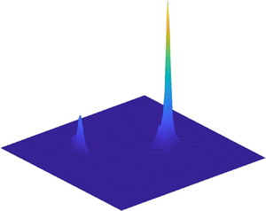In Yilmaz & Rickard (Reference Yilmaz and Rickard2004), it was found that in the approximate WDO case, the instantaneous DUET estimates $\tilde a(\tau ,\omega ), \tilde \delta (\tau ,\omega )$ (equations (2.11) and (2.13)) are not identically related to the actual mixing parameters $(\alpha _j, \delta _j)$ of the original $N_s$ sources, but they cluster around them. Therefore, the realization of (2.14) is obtained by construction of a two-dimensional weighted histogram for determining these clusters. The histogram domain, $I(\alpha ,\delta )$, is defined over $\tilde a(\tau ,\omega ), \tilde \delta (\tau ,\omega )$ as follows:

(2.16)\begin{equation} I(\alpha,\delta)\triangleq \{ (\tau, \omega ) \mid |\tilde\alpha (\tau,\omega)-\alpha |<\varDelta_\alpha, | \tilde\delta (\tau,\omega )-\delta |<\varDelta _\delta \}, \end{equation}

where $\varDelta _\alpha$ and $\varDelta _\delta$ are smoothing resolution widths. Using the $\tilde a(\tau , \omega ), \tilde \delta (\tau , \omega )$ pairs to indicate the indices of the histogram and using $|{\hat x}_1(\tau , \omega ){\hat x}_2(\tau , \omega ) |^p \omega ^q$ for the weight, a two-dimensional weighted histogram is constructed:

(2.17)\begin{equation} H( \alpha, \delta )\triangleq \iint_{(\tau, \omega ) \in I( \alpha, \delta )} | {{{\hat x}_1}(\tau ,\omega ){{\hat x}_2}(\tau, \omega )}|^p \omega ^q \,\textrm{d}\tau \,\textrm{d}\omega. \end{equation}

Here, $p$ and $q$ are variables of a weighted average, which, by default, are set to $p = 1$, $q = 0$ (Yilmaz & Rickard Reference Yilmaz and Rickard2004). If assumptions (i)–(v) hold, (2.17) takes the form

(2.18)\begin{equation} H(\alpha,\delta) =\begin{cases} \displaystyle\iint_{(\tau, \omega ) \in I( {\alpha, \delta } )} | {\hat s}_j(\tau, \omega ) |^{2p}{\omega ^q}\,\textrm{d}\tau \,\textrm{d}\omega & | \alpha _j - \alpha| < \varDelta _\alpha, \ | \delta _j - \delta |<\varDelta _\delta, \\ 0 & \text{otherwise}. \end{cases} \end{equation}

The weighted histogram separates and clusters the parameter estimates of each source. The number of peaks reveals the number of sources, and the peak locations reveal the associated source's anechoic mixing parameters, which are denoted by $(\tilde \alpha _j, \tilde \delta _j)$. Then, the relative estimated attenuation $\tilde a_j$ is retrieved from the estimated symmetric attenuation $\tilde \alpha _j$ by

(2.19)\begin{equation} \tilde a_j = \frac{ {\tilde \alpha}_j + \sqrt {{\tilde \alpha }_j^2 + 4} }{2}. \end{equation}

Next, $N_s$ estimated pairs $(\tilde \alpha _j, \tilde \delta _j)$ should be related back to each time–frequency point $(\tau ,\omega )$ which is closest to the local parameter estimates $(\tilde \alpha (\tau ,\omega ), \tilde \delta (\tau ,\omega ))$. Following Yilmaz & Rickard (Reference Yilmaz and Rickard2004), a maximum-likelihood association rule (estimator) for the $j$th source is obtained as

(2.20)\begin{equation} J(\tau, \omega )\triangleq \arg\min_j \frac{ | {\tilde a}_j \ \textrm{e}^{ - \textrm{i} {\tilde \delta }_j \omega }{\hat x}_1(\tau, \omega ) - {\hat x}_2(\tau, \omega ) |^2 }{ 1 + {\tilde a}_j^2 }. \end{equation}

These obtained estimators are used to obtain $N_s$ binary masks, as follows:

(2.21)\begin{equation} {\tilde M}_j(\tau,\omega) =\begin{cases} 1 & J(\tau, \omega) = j, \\ 0 & \text{otherwise}, \end{cases} \end{equation}

and the maximum-likelihood source estimates are obtained, as proposed in Yilmaz & Rickard (Reference Yilmaz and Rickard2004), based on maximum-likelihood estimates of $(\tilde \alpha _j, \tilde \delta _j)$, as

(2.22)\begin{equation} \hat{s}_j(\tau, \omega ) = {\tilde M}_j(\tau, \omega )\frac{ {\hat x}_1(\tau, \omega) + {\tilde a}_j \ \textrm{e}^{\textrm{i}{\tilde \delta}_j\omega}{\hat x}_2(\tau, \omega) }{ 1 + {\tilde a}_j^2 }. \end{equation}

In summary, implementing DUET consists of the following main steps (we assume that two mixtures are acquired):

1. (i) Construct time–frequency representations of both mixtures: $\hat {x}_1(\tau ,\omega )$, $\hat {x}_2(\tau ,\omega )$.

2. (ii) Extract local mixing-parameter estimates: $\tilde {a}(\tau ,\omega )$, $\tilde {\delta }(\tau ,\omega )$.

3. (iii) Out of the set of local mixing-parameter estimates, form $N_s$ parameter pairings, optimally corresponding to the true mixing-parameter pairings: $(\tilde {a}_1, \tilde {\delta }_1), \ldots , (\tilde {a}_{N_s}, \tilde {\delta }_{N_s})$.

4. (iv) For each determined mixing-parameter pair, generate a binary mask corresponding to the time–frequency points that yield that particular mixing-parameter pair: $M_1(\tau ,\omega ), \ldots , M_{N_s}(\tau ,\omega )$.

5. (v) Isolate (demix) the sources by applying each mask to both mixtures. This yields: $\hat {s}_{1}(\tau ,\omega ),\ldots ,\hat {s}_{N_s}(\tau ,\omega )$.

6. (vi) Finally, transform each demixed time–frequency representation to the time domain, yielding the isolated sources $s_{1}(t), \ldots , s_{N_s}(t)$.

In the following we extend the DUET-based method to also determine the propagation velocity vector of each of the identified sources.

3.1. Method derivation

Our approach for source propagation direction determination derives from that of Oshman & Markley (Reference Oshman and Markley1999), where a global positioning system (GPS) antenna array is used for spacecraft attitude estimation, based on measuring the phase difference between GPS signals acquired by the antenna array.

Consider a source $s$ that propagates in the $x$–$z$ plane with velocity

(3.1)\begin{equation} \boldsymbol{u}_{} = u_{} \hat{\boldsymbol{u}}_{}, \end{equation}

where the source speed is $u= | {\boldsymbol {u}}|$ and $\hat { {\boldsymbol {u}}}$ is a unit directional vector. Our goal is to determine this velocity (both direction and magnitude) for each source from source mixtures measured by $N$ sensors.

We position $N$ sensors in the flow located at $\boldsymbol {r}_{x_{i}}$, $i=1, \ldots , N$, in the $x$–$z$ plane ($N=3$ in figure 1). Analogously to the GPS antenna array of Oshman & Markley (Reference Oshman and Markley1999), we denote sensor 1 as the master sensor and, accordingly, sensors $2,\ldots , N$ as the slave sensors. This sensor array configuration defines $N-1$ baseline vectors, $\boldsymbol {r}_{x_{i}} - \boldsymbol {r}_{x_{1}}$, $i=2, \ldots , N$. As in GPS attitude determination problems, here, too, a minimum of two baselines are required, corresponding to a minimal configuration of three sensors.

The source $s$ that travels from the master sensor (sensor 1) to slave sensor $i$, $i=2, \ldots , N$, covers the distance

(3.2)\begin{equation} ({\boldsymbol{r}}_{x_i} - {\boldsymbol{r}}_{x_1})^\textrm{T} \hat{{\boldsymbol{u}}} = \delta_{i} u, \quad i=2, \ldots, N, \ N\ge 3, \end{equation}

where we have used a shorthand notation for the delay $\delta _i$, and $\delta _{i} > 0$ ($\delta _{i} < 0$ with the same magnitude if the source travels in the opposite direction). We now use the normalized baseline vectors to define the rows of the matrix ${\boldsymbol{\mathsf{W}}} \in \mathbb {R}^{N-1,2}$:

(3.3)\begin{equation} {\boldsymbol{\mathsf{W}}} \triangleq \begin{bmatrix} \delta_{2}^{{-}1} (\boldsymbol{r}_{x_{2}} - \boldsymbol{r}_{x_{1}})^\textrm{T} \\ \delta_{3}^{{-}1} (\boldsymbol{r}_{x_{3}} - \boldsymbol{r}_{x_{1}})^\textrm{T}\\ \vdots\\ \delta_{N}^{{-}1} (\boldsymbol{r}_{x_{N}} - \boldsymbol{r}_{x_{1}})^\textrm{T} \end{bmatrix}. \end{equation}

Then, (3.2) can be rewritten as

(3.4)\begin{equation} u^{{-}1} {\boldsymbol{\mathsf{W}}} \hat{\boldsymbol{u}}_{}={\boldsymbol{1}}, \end{equation}

where all entries of the vector $ {\boldsymbol {1}} \in \mathbb {R}^{N-1}$ are ones. Equation (3.4) is a system of $N-1$ linear equations for the speed $u_{}$ and the independent entry of the direction vector $\hat {\boldsymbol {u}}_{}$. For $N=3$, this system has a unique solution if the columns of ${\boldsymbol{\mathsf{W}}}$ are independent, which corresponds to a three-sensor configuration having two non-collinear baselines. For $N>3$, the system becomes overdetermined, calling for a least squares solution, a minimum-norm version of which is provided by the Moore–Penrose pseudoinverse of ${\boldsymbol{\mathsf{W}}}$, which can be robustly computed using the singular value decomposition.

3.2. Sensor configuration design

Relative to some given disturbance direction, the configuration of the $N$ sensors determines the numerical properties of the linear system (3.4), which, in turn, determine the quality of the solution for the disturbance propagation velocity. We use the condition number of the coefficient matrix, denoted as ${\kappa ({\boldsymbol{\mathsf{W}}})}$, which is the ratio between the largest and smallest singular values of ${\boldsymbol{\mathsf{W}}}$, as a measure of the quality of the solution. A small condition number, i.e. a condition number close to one, means that the system is well-conditioned, and a high-quality solution may be expected. On the other hand, a large condition number is associated with an ill-conditioned system, leading to a solution of poor quality, due to system sensitivity to small input errors.

Evaluating the condition number as a function of the sensor configuration and disturbance direction can naturally assist in the following two sensor design tasks:

1. (i) Given a certain sensor configuration, ${\kappa ({\boldsymbol{\mathsf{W}}})}$ can be used to find the unobservable directions; that is, the disturbance directions that cannot be identified using the given configuration.

2. (ii) Given the disturbance direction, ${\kappa ({\boldsymbol{\mathsf{W}}})}$ can be used to design the best sensor configuration for the task of disturbance velocity estimation.

In what follows, we demonstrate the above two tasks via illustrative examples.

3.2.1. Unobservable directions for a given sensor configuration

In this subsection, we demonstrate how the ${\kappa ({\boldsymbol{\mathsf{W}}})}$ measure may assist in finding the unobservable directions associated with a given three-sensor configuration. The disturbance speed is set to be $| {\boldsymbol {u}}|=1$ m s$^{-1}$ and the velocity direction, represented by the angle $\theta$ with respect to $\hat { {\boldsymbol {e}}}_x$ as displayed in figure 1, is varied between 0$^\circ$ and 360$^\circ$ at 4001 points uniformly spread in this range.

In the top three panels of figure 2, we illustrate three different three-sensor configurations, all consisting of a master sensor 1 (marked by the symbol $\times$) and two slave sensors 2 and 3 (marked as small circle and square, respectively). The two baselines are illustrated by arrows, pointing from the master sensor to the slave sensors. The bottom three panels of figure 2 present the value of the ${\kappa ({\boldsymbol{\mathsf{W}}})}$ measure on polar coordinates as a function of $\theta$, the disturbance arrival direction. The radial distance from the origin stands for the value of ${\kappa ({\boldsymbol{\mathsf{W}}})}$, and the two circles in each of these plots correspond to the values of ${\kappa ({\boldsymbol{\mathsf{W}}})}=2.5$ (inner dotted circle) and ${\kappa ({\boldsymbol{\mathsf{W}}})}=5$ (outer circle). Disturbance arrival angles corresponding to ${\kappa ({\boldsymbol{\mathsf{W}}})} \ge 50$ are marked in these plots by red arcs on the outer circle. The ill-conditioning threshold value of 50 is arbitrarily chosen; clearly, disturbance sources arriving from directions corresponding to angles within the red arcs may not be determined correctly. As may be expected, figure 2(c) reveals that when the two baselines are collinear, the entire polar domain is unobservable.

Figure 2.

Unobservable directions for (a–c) three sensor configurations. Top panels: sensor configurations. Master sensor marked by $\times$, slave sensors marked by circle and square symbols, baselines denoted by arrows. Bottom panels: polar plots of ${\kappa ({\boldsymbol{\mathsf{W}}})}$ versus disturbance arrival direction. Angles associated with ${\kappa ({\boldsymbol{\mathsf{W}}})} \ge 50$ are shown via red arcs on the outer circles (that correspond to ${\kappa ({\boldsymbol{\mathsf{W}}})}=5$).

3.2.2. Best sensor configuration for a given disturbance direction

We next demonstrate how the ${\kappa ({\boldsymbol{\mathsf{W}}})}$ measure is used to design the optimal sensor configuration for a given disturbance direction. The disturbance speed is set to $| {\boldsymbol {u}}_j| =1$ m s$^{-1}$ and the disturbance arrival angle varies between (a) $\theta = -90^\circ$, (b) $\theta = -60^\circ$, (c) $\theta = -20^\circ$ and (d) $\theta = 0^\circ$. Two sensors are fixed, whereas the location of the third sensor varies within the range $x,z \in [-50, 50]$ mm, with 1 mm step in each direction. Figure 3 displays the value of ${\kappa ({\boldsymbol{\mathsf{W}}})}$ for all possible locations of the third sensor in the $x$–$z$ plane. Regions of the $x$–$z$ plane associated with high values of ${\kappa ({\boldsymbol{\mathsf{W}}})}$ should be avoided. In figure 3(d), the first slave sensor is located such that its baseline is perpendicular to the disturbance velocity vector, which results in $\delta _{12}= 0$. Therefore, ${\kappa ({\boldsymbol{\mathsf{W}}})} \to \infty$ for any location of the second slave sensor, rendering the determination of the velocity vector in this configuration impossible. In general, figure 3(d) demonstrates that the problem becomes unobservable if the sensors are configured such that either (1) at least one baseline is perpendicular to the disturbance velocity vector or (2) the baselines are collinear.

Figure 3.

The ${\kappa ({\boldsymbol{\mathsf{W}}})}$ measure as a function of the location of the third sensor, when the first two sensors (marked by the $\times$ and circle symbols) are fixed, for four different disturbance arrival angles: (a) $\theta = -90^\circ$, (b) $\theta = -60^\circ$, (c) $\theta = -20^\circ$ and (d) $\theta = 0^\circ$. The disturbance velocity vector is represented by the green arrow and the baseline vector between the first two sensors is denoted by the blue arrow.

4.1. Generating disturbance source model via LST

We consider incompressible wall-bounded parallel shear flow with streamwise direction ($x$), wall-normal direction ($y$) and spanwise direction ($z$). We decompose the total velocity field into a base flow of the form $ {\boldsymbol {U}}= [U(y) \ \ 0 \ \ 0]^\textrm {T}$ and perturbed ($ {\boldsymbol {u}}^{(1)}$, $p^{(1)}$) states about the base flow. All quantities are non-dimensionalized by the free-stream velocity, $U_\infty$, and the boundary layer displacement thickness, $\delta _d$, at a given streamwise position. This renders the Reynolds number $Re=U_\infty \delta _d/\nu$ as the governing parameter, where $\nu$ is the kinematic viscosity of the flow. The linearized Navier–Stokes equations are obtained by subtracting the equations for the base state from those corresponding to the total state, and dropping the nonlinear terms.

We analyse the stability of the mean flow with respect to wavelike velocity and pressure perturbations, also known as normal modes, for which

(4.1)\begin{equation} q^{(1)} =\hat{q} ( y ) \ \textrm{e}^{\textrm{i} ( \alpha x+\beta z-\omega t )}, \end{equation}

where $q^{(1)}=[u^{(1)} \ \ v^{(1)} \ \ w^{(1)}\ \ p^{(1)}]^\textrm {T}$, and $\hat {q}(y)=[ \hat {u}(y) \ \ \hat {v}(y) \ \ \hat {w}(y) \ \ \hat {p}(y)]^\textrm {T}$ is the corresponding complex eigenvector. We consider the spatial case in which $\alpha$ is a complex eigenvalue; $\alpha _r\triangleq \textrm {Re}(\alpha )$ and $\beta$ are the disturbance streamwise and spanwise wavenumbers, respectively; $\alpha _{im}\triangleq \textrm {Im}(\alpha )$ is the disturbance streamwise decay/growth rate for positive and negative values, respectively; and $\omega$ is the dimensionless disturbance frequency. Substituting (4.1) into the linearized Navier–Stokes equations (which is equivalent to taking the Fourier transform) results in the following dispersion relation:

(4.2)\begin{equation} \mathbb{D} (\alpha, \beta, \omega) = 0. \end{equation}

This constitutes an eigenvalue problem for the complex eigenvalue $\alpha$ and its corresponding eigenfunction $\hat {q}$, for the given spanwise wavenumber $\beta$, the real frequency $\omega$, the Reynolds number $Re$ and the base flow velocity profile $U(y)$.

Following the primitive variable formulation in Schmid & Henningson (Reference Schmid and Henningson2001, p. 290), the dispersion relation (4.2) for the spatial case translates to the following system of equations:

(4.3)\begin{equation} \begin{bmatrix} 0 & -D & -\textrm{i}\beta & 0 & 0 & 0 \\ 0 & 0 & 0 & 0 & 1 & 0 \\ 0 & 0 & 0 & 0 & 0 & 1 \\ C & T & \textrm{i} U \beta & 0 & -D/Re & -\textrm{i}\beta/Re \\ 0 & -Re C & 0 & {Re}D & Re U & 0 \\ 0 & 0 & -Re C & \textrm{i}\beta Re & 0 & Re U \end{bmatrix} \begin{bmatrix} {\hat{u}} \\ {\hat{v}} \\ {\hat{w}} \\ {\hat{p}} \\ {\hat{v}_x} \\ {\hat{w}_x} \\ \end{bmatrix}=\textrm{i}\alpha \begin{bmatrix} {\hat{u}} \\ {\hat{v}} \\ {\hat{w}} \\ {\hat{p}} \\ {\hat{v}_x} \\ {\hat{w}_x} \\ \end{bmatrix}, \end{equation}

with homogeneous boundary conditions. For example, in BBL, $\hat {u} = \hat {v} = \hat {w} = \hat {v}_x = \hat {w}_x = 0$ at $y=0$ and $y\to \infty$ (see figure 4). Here $C$ and $T$ denote the linear operators $C \triangleq \textrm {i}\omega + (D^2 - \beta ^2 )/Re$ and $T \triangleq U D -U_y$. Both subscript $(\cdot )_y$ and operator $D$ denote the first derivative with respect to $y$, whereas $(\cdot )_x$ denotes the first derivative with respect to $x$.

Figure 4.

Flow over a flat plate.

Thus, we have a boundary value problem for the above system, which we solve numerically with the aid of Matlab, utilizing spectral methods (Trefethen Reference Trefethen2000) with $150$ grid points. The results of the numerical dispersion relation solution are validated against reported results in the literature for the BBL (Jordinson Reference Jordinson1970; Schmid & Henningson Reference Schmid and Henningson2001; Boiko et al. Reference Boiko, Dovgal, Grek and Kozlov2011). We search for the most unstable TS wave, where its eigenmode is obtained from (4.3), and its amplitude profile is represented by the corresponding $|\hat {q}(y)|$.

In addition to TS waves we also consider WP sources. A single WP disturbance may be generated by a short pulse actuation of the boundary layer at a specific location. The short pulse generates a localized disturbance that may be regarded as a linear superposition of many TS waves associated with a wide range of frequencies that may grow or decay downstream in the boundary layer. We focus on the long-time instability characteristics of the WP, far away from the pulse actuation location, after the WP transient behaviour has decayed. Each of the WP modes travels with its own phase velocity, given by

(4.4)\begin{equation} {\boldsymbol{c}}_r=[c_x \quad c_z]^\textrm{T}= {\boldsymbol{k}} \frac{\omega}{|{\boldsymbol{k}}|^2}, \end{equation}

but all modes share the same group velocity:

(4.5)\begin{equation} {\boldsymbol{c}}_g=\nabla _k\omega. \end{equation}

In (4.5), $\nabla _k=[{\partial }/{\partial \alpha }\ \ {\partial }/{\partial \beta }]^\textrm {T}$ and $ {\boldsymbol {k}}$ is a real wavenumber vector, defined as

(4.6)\begin{equation} {\boldsymbol{k}} \triangleq [\textrm{Re}\{\alpha\} \quad \beta]^\textrm{T}, \end{equation}

i.e. $c_x=\textrm {Re}\{\alpha \}\omega /| {\boldsymbol {k}}|^2$ and $c_z=\beta \omega /| {\boldsymbol {k}}|^2$.

Following the theoretical model proposed in Gaster (Reference Gaster1975), the model for a single three-dimensional WP source in non-parallel shear flow is given by

(4.7)\begin{align} &u_{WP}(x,y_0,z,t) \nonumber\\ &\quad = A(y_0)\ \textrm{Re}\left\{ x^{ - 1/4}\sum_{{\omega _n} = {\omega _0}}^{{\omega _N}}\sum_{{\beta _k} = {\beta _0}}^{{\beta _M}} {\exp{ {\textrm{i}\left[ {\int_{{x_0}}^x {\alpha ( {\zeta, \beta _k,{\omega _n}} )} \,\textrm{d}\zeta+\beta_k (z-z_0) - \omega_n t} \right]}}} \right\}, \end{align}

where $u_{WP}(x,y_0,z,t)$ is the streamwise velocity of the WP at a given wall-normal height $y_0$, $(x_0, z_0)$ is the location where the WP source is generated and $(x, z)$ is the location where the WP source is measured. In our case of flow over a flat plate, the origin of the $x$ axis is at the plate's leading edge. The term $x^{-1/4}$ has been included to compensate for the slight divergence of the mean flow (a model that accounts for downstream eigenfunction variation is provided in Cohen (Reference Cohen1994)). Under the parallel flow assumption, we obtain

(4.8)\begin{align} u_{WP}(x,y_0,z,t) =A(y_0)\ \textrm{Re}\left\{ \sum_{{\omega _n} = {\omega _0}}^{{\omega _N}}\sum_{{\beta _k} = {\beta _0}}^{{\beta _M}} {\exp \{ {\textrm{i}[ {\alpha_{x_0,\omega_n,\beta_k}(x - x_0) + \beta_k (z-z_0) - \omega_n t} ]} \}} \right\}. \end{align}

Here, the eigenvalue $\alpha _{x_0}$ associated with $\omega _n,\beta _k$ is kept constant along the streamwise direction. The model presented in (4.8) is a simplified version of the theoretical model proposed in Gaster (Reference Gaster1975) and Cohen (Reference Cohen1994). Its simplicity notwithstanding, this model provides estimates of the development of a WP disturbance over the relatively short distances between the sensors that are adequate for testing the performance of our DUET-based method prior to proceeding to experimental studies.

4.2. Using LST to model sensor measurement

We implement the LST model under the parallel flow assumption for generating simulated mixtures of $N_s$ disturbance sources that are measured by $N_x$ sensors. The disturbances considered comprise TS wave sources and WP sources. In the case of a single TS wave disturbance measured at a specific wall-normal height $y_0$, (4.1) can be written as

(4.9)\begin{equation} q(x,y_0,z,t) = |\hat{q}(y_0)|\ \textrm{e}^{-\alpha _{im}x}\cos (-\omega t+\phi_t(x,y_0,z)). \end{equation}

In (4.9) the phase shift in time, $\phi _t$, at $y_0$ is determined by the spatial parameters of the disturbance

(4.10)\begin{equation} \phi_t(x,y_0,z) \triangleq \alpha_r x + \beta z + \phi ({\hat{q}}(y_0)) + \phi _{t_0}, \end{equation}

where $\phi _{t_0}$ is the initial phase and $(x,z)$ are the current location coordinates.

A source is defined as the signal that would have been measured by a sensor if all other sources were nil (that is, when no other mechanically generated signal is sensed). Each source is generated by a particular physical disturbance generator, which characterizes its signature in the sensor recordings. The source $s_j$ is defined by its frequency $\omega _j$ and the initial phase $\phi _{t_{0_j}}$ it had at its introduction location ${ {\boldsymbol {r}}}_{s_j} = [l_x \ \ l_z]_{s_j}$ on the $x$–$z$ plane. Let ${ {\boldsymbol {r}}}_{x_i} = [l_x \ \ l_z]_{x_i}^\textrm {T}$ be the location of sensor $i$ on the $x$–$z$ plane, where $x_i$ stands for the signal measured by that sensor.

Using (4.9) and (4.10), we represent the measurement of source $s_j$ by sensor $i$ as

(4.11)\begin{equation} s_{ij}= |\hat{q}_j([l_y]_{x_i})|\ \textrm{e}^{-\alpha_{im_j}([l_x]_{x_i}-[l_x]_{s_j})} \cos(-\omega_j t+\phi_{t_{ij}}), \end{equation}

where $\phi _{t_{ij}}$, the phase of source $s_j$ as measured by sensor $i$, is given by

(4.12)\begin{equation} \phi _{t_{ij}} = \alpha _{r_j}([l_x]_{x_i}-[l_x]_{s_j}) + \beta _j([l_z]_{x_i}-[l_z]_{s_j}) + \phi _j([l_y]_{x_i}) + \phi _{t_{0j}}. \end{equation}

In (4.12), $[l_x]_{x_i}-[l_x]_{s_j}$ and $[l_z]_{x_i}-[l_z]_{s_j}$ are the downstream and spanwise distances, respectively, that the disturbance $s_j$ travels from its generation point to sensor $i$. The variation in the phase of source $s_j$ at the recording location of sensor $i$ is due to the spatial wavenumbers $\alpha _{r_j}$, $\beta _j$, and the eigenvector phase $\phi _j(y)$ of the source $s_j$ at the vertical location $[l_y]_{x_i}$ of sensor $i$.

Similarly, for a WP source generated at ${ {\boldsymbol {r}}}_{s_j}$ and measured by sensor $i$, we have

(4.13)\begin{align} s_{ij}= \textrm{Re}\left\{ \sum_{\omega _n = \omega _0}^{\omega _N}\sum_{\beta _k = \beta _0}^{\beta _M} \exp \{ \textrm{i}[ \alpha_{ x_{s_j},\omega _n,\beta _k } ( [l_x]_{x_i} - [l_x]_{s_j} ) + \beta_k ([l_z]_{x_i} - [l_z]_{s_j}) - \omega_n t ] \} \right\}. \end{align}

Finally, the source mixture measured by sensor $i$ in the presence of $N_s$ sources is

(4.14)\begin{equation} x_i = \sum_{j = 1}^{N_s} s_{ij},\quad i = 1,2,\ldots N_x. \end{equation}

Equation (4.14) provides a general model for a system consisting of $N_x$ sensors measuring $N_s$ TS and WP disturbance sources, represented by (4.11) and (4.13), respectively.

4.3. Numerical settings and procedure

The dispersion relation is solved for $\alpha$ and $q$ for the given frequency $\omega$, spanwise wavenumber $\beta$, Reynolds number $Re$ and base flow velocity profile $U(y)$ of BBL under the quasi-parallel flow assumption. We consider air flow at room temperature with kinematic viscosity $\nu = 0.15\times 10^{-4}$ m$^2$ s$^{-1}$, and the free-stream velocity is set to $U_{\infty }=5$ m s$^{-1}$. The disturbance sources are introduced at various downstream locations ($ {\boldsymbol {r}}_{s_j}$) with various frequencies. Each given pair of frequency and downstream injection location of each source is associated with the corresponding non-dimensional frequency $\omega$ and the local Reynolds number, which is based on the local displacement thickness, i.e. $Re(x)= U_\infty \delta _d(x)/\nu$ (for BBL the displacement thickness is given by $\delta _d(x) = 1.7208 \sqrt {\nu x/U_\infty }$). These are used to solve the dispersion relation for the spatial case. The sensors are set to measure the streamwise component of the flow, $u$. The obtained eigenvalues $\alpha$ and eigenfunctions $\hat u$ are used as inputs to the truth model, which consists of simulated source mixtures, measured by the sensors in the LST model. The simulations are performed in dimensional form, where the dimensionless parameters $\omega$ and $\alpha$ of each source are dimensionalized using the local displacement thickness at the injection location of the source and $U_{\infty }$. For simplicity and clarity of exposition, the non-parallel effect is neglected in our truth model, where it is assumed that the source eigenvalues and eigenfunctions remain unchanged during their downstream propagation towards the sensors. In reality, the non-parallel effect may significantly modify the amplitudes and phases of the sources at the location of the sensor, if the sources travel a long distance (many wavelengths) from their respective injection locations to the sensor. Nevertheless, the downstream distance between two neighbouring sensors, a key variable in the DUET method, is extremely small, compared with the disturbance wavelength. Therefore, the non-parallel effect is deemed negligible in our study, which is aimed at demonstrating the viability of the DUET method.

4.4. The DUET settings

The signals are acquired at a 1 kHz sample rate. In order to apply DUET to the two measured mixtures, we set the initial values of the DUET parameters for flow measurements according to those recommended for speech mixtures by Rickard (Reference Rickard2007).

1. (i) Window size. The window size of the short Fourier transform is set to 256 ms. The window size is important for good DUET performance and description of the frequencies in the flow. Increasing the window size will result in good frequency localization in the time–frequency domain, but the time localization will deteriorate. Too narrow a window size will result in a poor frequency resolution, but will increase the time resolution. In Rickard (Reference Rickard2007), it was found that speech is most window-disjoint orthogonal when a window of 1024 samples is used, corresponding to a length of 64 ms. In our study of shear flows, we found that good window sizes appropriate for time scales in our measurements are of 128–512 ms in length, corresponding to 128–512 samples at 1 kHz sample rate. This range results in a trade-off between frequency and time resolution (128 samples in favour of time resolution and 512 samples in favour of frequency resolution).

2. (ii) Histogram domain. The histogram domain $I(\alpha ,\delta )$ is divided into 105 bins by 150 bins. The smoothing resolutions ($\varDelta _\alpha$ and $\varDelta _\delta$) are set such that the weighted clusters of peaks that emerge on the histogram domain, centred on the actual mixing parameter pairs, are smoothed with a 3-by-3 neighbouring-bins window. This facilitates determination of localized histogram peaks.

3. (iii) Histogram weights. Motivated by the maximum-likelihood symmetric attenuation estimator in Yilmaz & Rickard (Reference Yilmaz and Rickard2004), we set $p=1$ and $q=0$. Good DUET performance is also obtained by setting $p=2$ and $q=0$, to reduce delay estimator bias (Yilmaz & Rickard Reference Yilmaz and Rickard2004).

Next, two numerical examples are presented to study DUET performance when using various sensor configurations in various source mixing scenarios. The first example, which addresses five two-dimensional sources with two sensors placed at different heights, tests DUET as a source separation method. The second example, which addresses three three-dimensional sources with different propagation directions, sampled by a configuration of three sensors sharing the same height, tests the method's performance on each separated source.

4.5. Example 1: disturbance mixture separation

This example serves to test and demonstrate the capabilities of DUET as a source identification and separation method in boundary layer measurement applications. To this end, our truth model comprises a five-source mixture, introduced upstream of the sensors. In particular, $s_1$ and $s_4$ are two-dimensional WPs introduced at downstream locations $x=0.36$ m and $x=1.0$ m (recall that the origin, $x=0$, is located at the plate's leading edge). These locations correspond to Reynolds numbers $Re_1=600$ and $Re_4=1000$, respectively. The sources $s_2$, $s_3$ and $s_5$ are two-dimensional TS waves, introduced at downstream locations $x=0.25$ m, $x=2$ m and $x=0.57$ m, corresponding to $Re_2=500$, $Re_3=1400$ and $Re_5=750$, respectively. The TS source dimensionless frequencies are $\omega _2=0.12$, $\omega _3=0.04$ and $\omega _5=0.07$, corresponding to 63.7, 7.6 and 24.8 Hz, respectively. The stability properties of the sources are illustrated in figure 5.

Figure 5.

Truth-model sources. WP sources $s_1$ (magenta dashed line) and $s_4$ (cyan dashed line) at specific $Re$; TS source eigenvalues, denoted by asterisk symbols: $\alpha _{s_2} =0.3014 + 0.0006\textrm {i}$ (red), $\alpha _{s_3} =0.1347 + 0.0009\textrm {i}$ (green) and $\alpha _{s_5} =0.2010 + 0.0002\textrm {i}$ (blue) at specific ($Re$, $\omega$). Sources plotted over contours of constant streamwise wavenumber $\alpha _r$ (dotted black contours), growth rate $\alpha _{im}$ (solid black contours). The neutral curve is denoted by the bold black contour.

The sensors are located at $[l_x]_{x_1} = 2.29$ m and $[l_x]_{x_2} = [l_x]_{x_1} + 0.005$ m. The downstream separation of 0.005 m between the sensors is chosen to satisfy the fourth underlying assumption of the DUET method. Accordingly, figure 5 shows that the slowest TS disturbances propagate at a velocity of approximately $(c_r)_{max}\approx 0.3U_\infty$, and the maximal frequency in the simulated mixture (see figure 7), associated with TS source $s_2$, is $\,f_m=\,f_{2} = 63$ Hz. Using (2.6) yields $|[l_x]_{x_1} - [l_x]_{x_2}| < {{\rm \pi} c_r}/{\omega _m}={0.3U_\infty }/{2f_m}\approx 0.0118$ m, rendering an upper bound on the limiting distance between the sensors. We place each sensor at a different height above the plate: sensor 1 at 2 mm and sensor 2 at 1.4 mm. The simulated TS eigenfunction profiles (amplitude and phase of the streamwise disturbance velocity) are shown in figure 6, where the sensor positions are indicated by the horizontal lines (near the inner maximum of the streamwise component of the TS disturbance profiles).

Figure 6.

Streamwise component ($u$) of the three TS sources: $s_2$ (red), $s_3$ (green) and $s_5$ (blue). (a) Eigenfunction amplitude (normalized by its maximum) and (b) eigenfunction phase. Black lines: height of sensor 1 (solid) and sensor 2 (dashed). The sensor heights are related to the correct positions at the eigenfunction profiles of the sources by rescaling the $y$ axis with the average $\delta _d$ of all injection locations of the TS sources.

Figures 7(a) and 7(d) display the outputs of two sensors that are used to measure the streamwise velocity component over a 2 s time interval. The corresponding Fourier transforms are shown in figures 7(b) and 7(e), and the spectrograms of the mixtures are shown in figures 7(c) and 7(f), respectively. Examination of figures 7(b) and 7(e) reveals that each measured mixture contains the frequencies of the introduced sources. Each TS source has a unique single frequency, whereas the WP typical spectrum looks like a bell-shaped signature centred about a dominant frequency of around 50 Hz for $s_1$ and 24 Hz for $s_4$. Figures 7(c) and 7(f) demonstrate that the second DUET assumption (WDO) is not fully satisfied. Specifically, the WP source $s_1$ and the TS source $s_2$ co-dominate the flow for a certain time–frequency range. Similarly, but to a lesser degree, the WP source $s_4$ and the TS source $s_5$ coexist for a certain time–frequency range.

Figure 7.

True (LST-computed) mixtures as measured by two sensors: (a) $x_1$ and (d) $x_2$. Corresponding Fourier transforms: (b) $E_{x_1}$ and (e) $E_{x_2}$. Absolute values of windowed Fourier transforms (spectrograms), for which a window of 256 samples is used: (c) $20\log (|\hat {x}_1|+10^{-6})$ dB and (f) $20\log (|\hat {x}_2|+10^{-6})$ dB.

Figure 8 shows that the DUET-based method successfully identifies the correct number of sources. The isometric view of the histogram, presented in figure 8(b), shows five peaks associated with five true sources. Three peaks are related to the three TS sources and the other two peaks are associated with the WP sources. Figure 8(a) displays the mixing-parameter pairs of the true (LST-computed) TS sources, together with the peak contours. Clearly, three of the histogram peaks coincide with the mixing parameters of the true TS sources, $s_2$, $s_3$ and $s_5$. The other two peaks are associated with the WP sources, $s_1$ and $s_4$. In this example, histogram peaks are clustered around similar values of $\delta$. The height difference between sensors has a strong effect on the $\alpha$ parameter. Thus, placing the sensors at different heights increases the scatter along the $\alpha$ axis, which facilitates distinguishing between the histogram peaks.

Figure 8.

A DUET two-dimensional cross power weighted $(p = 1, q = 0)$ histogram of symmetric attenuation $\alpha =(a - 1/a)$ and delay estimate pairs from two mixtures of five sources. (a) Contour plot (black) of the two-dimensional histogram with corresponding true (LST-computed) mixing parameter pairs for each TS source: $s_2$ (red), $s_3$ (green) and $s_5$ (blue). (b) Isometric view.

Obtained from the histogram peak locations, the identified mixing parameters are used to demix the sources. Figure 9 shows five estimated sources, denoted by $y_j$, $j=1,2,3,4,5$, as identified by the DUET method. Figures 9(a) and 9(j) depict the time signatures of the estimates of sources $s_1$ and $s_4$, clearly featuring typical WP structures. Nonetheless, figure 9(l) shows that the estimate of WP source $s_4$ contains a weak spurious signal at 50 Hz. This frequency is also shared by TS source $s_5$. Figure 9(m–o) shows that the spectrum of the estimate of TS source $s_5$ is not contaminated by the estimates of other sources. However, it is attenuated in the region where WP source $s_4$ is active. Figure 9(g–i) indicates that the estimate of TS source $s_3$ contains very weak signatures (50 dB) of $s_4$, which do not affect its time signature. In this example we verified that multiple WP and TS disturbance sources in shear flows (sufficiently) satisfy the WDO condition, thus allowing accurate mixing parameter estimation with only two sensors, which yields high-fidelity signal recovery using DUET.

Figure 9.

The DUET estimates of sources: (a) $y_1$, (d) $y_2$, (g) $y_3$, (j) $y_4$ and (m) $y_5$. Corresponding Fourier transforms: (b) $E_{y_1}$, (e) $E_{y_2}$, (h) $E_{y_3}$, (k) $E_{y_4}$ and (n) $E_{y_5}$. Corresponding spectrograms (dB): (c) $|\hat {y}_1|$, (f) $|\hat {y}_2|$, (i) $|\hat {y}_3|$, (l) $|\hat {y}_4|$ and (o) $|\hat {y}_5|$.

4.6. Example 2: disturbance velocity estimation

This example is used to demonstrate how our DUET-based method can be used to estimate the propagation velocity of disturbances in the flow using only three sensors, appropriately placed in the flow field. As in the previous example, LST is used for generating a truth model comprising a mixture of three sources: two three-dimensional TS (oblique) waves and one two-dimensional WP source. The three disturbance sources are introduced at different locations upstream of the sensors, as detailed in table 1, which also lists the source parameters.

Table 1.

Disturbance sources.

The frequencies of the TS sources $s_2$ and $s_3$ are 53.1 and 22.7 Hz, respectively. Their corresponding eigenvalues are obtained by solving the dispersion relation for the spatial case, which results in $\alpha _2 = 0.2987 + 0.0003\textrm {i}$ and $\alpha _3= 0.1613 + 0.0039\textrm {i}$. The propagation angle of a TS source is given by

(4.15)\begin{equation} \theta=\arctan\left(\frac{\beta}{\textrm{Re}\{\alpha\}}\right), \end{equation}

which yields $26.7^\circ$ for $s_2$ and $-42.9^\circ$ for $s_3$. The angle of the two-dimensional WP ($\beta =0$) source $s_1$ is $0^\circ$. The propagation velocities of the TS sources correspond to their phase velocities as given by (4.4) from which we obtain that the TS waves travel at speeds $c_2= 1.7950$ m s$^{-1}$ and $c_3= 1.3618$ m s$^{-1}$ along their respective wave vector directions. In the case of the WP source, each of its many modes propagates with its own phase velocity, which differs from those of the other modes, but all travel as a group of waves at a group velocity $ {\boldsymbol {c}}_g$, also known as the WP envelope velocity. This velocity can be obtained by monitoring the leading edge and the trailing edge of the WP envelope in the $t$–$x$ domain (Gaster Reference Gaster1975). For $Re=851$ it is shown in Gaster & Grant (Reference Gaster and Grant1975) that the leading edge of a three-dimensional WP propagates at 0.44 of the free-stream value, whereas the trailing edge seems to exhibit some local transient behaviour near the source before settling down to a path with a slope of 0.36$U_{\infty }$. In particular, figure 10 shows the velocity of the WP in our simulation. In this figure we denote the time when the maximum value of the envelope (maximum of $|u_{WP}(t,x)|$) occurs at each downstream location of the sensors. The slope of the linear function fitting the three points on the $t$–$x$ plane represents the speed of the WP travelling in the streamwise direction, which, in our simulation, is 2.1901 m s$^{-1}$.

Figure 10.

Plot of $\arg \max |u_{WP}(t,L_x)|$ for each sensor on the $t$–$x$ domain, where $x$ is the distance from the leading edge and $t_0$ is the pulse start time. The slope of the fitted linear function represents the envelope velocity of the WP source.

The sensors are located at $ {\boldsymbol {r}}_{x_1}= [796, \ 0]$ mm, $ {\boldsymbol {r}}_{x_2} = [[l_x]_{x_1} + 6, \ 5]$ mm and $ {\boldsymbol {r}}_{x_3} =[[l_x]_{x_1} + 9, \ 5]$ mm. They are placed at the same height above the plate, near the outer maximum of the streamwise component of the TS disturbance profiles.

The eigenfunction profiles (amplitude and phase of the streamwise disturbance velocities) of the two TS waves are shown in figure 11, where the sensors’ height above the plate is indicated by the horizontal line. As demonstrated in figure 11(b), each TS source has a vertical phase profile, with two distinct regions (near and away from the surface) separated by a jump with a value of ${\rm \pi}$. This jump occurs approximately between the inner and outer maximum of the eigenfunction amplitude profile (figure 11a).

Figure 11.

Streamwise component ($u$) of TS sources: $s_2$ (red) and $s_3$ (magenta). (a) Eigenfunction amplitude (normalized by its maximum) and (b) eigenfunction phase. The sensors’ vertical position is denoted by the horizontal black dashed line.

The phase profile of each source can result in false velocity angle estimation, because the phase change between the sensors is attributed to the source's horizontal propagation behaviour in our modelling framework. To overcome this problem, the sensors should be placed either (1) at the same height, outside or inside the boundary layer, e.g. near the inner maximum of the disturbance streamwise velocity profile (for non-parallel flow this height should be updated along the constant streamline), or (2) in the outer part of the boundary layer (if known a priori), possibly at different heights, where the phase profile is constant.

Using DUET for disturbance velocity estimation, which is the focus of the present example, is a two-stage procedure, with the first stage consisting of disturbance separation and identification. Since the theory underlying this stage has been thoroughly exemplified via the previous example, we defer the details concerning this stage to Appendix A. Thus, in the following, we only address the results of the second stage of the velocity estimation procedure, relying on the results of the first stage as they are described in Appendix A.

In figure 12 we overlay the histogram obtained using sensors 1 and 3 (blue contours) over the histogram obtained using sensors 1 and 2 (black contours). As can be clearly observed, the blue contours are shifted to the right relative to the black ones, that is, $|\delta _{j12}| < |\delta _{j13}|$, which agrees with the position of sensor 3 being downstream of sensor 2.

Figure 12.

Top view of DUET two-dimensional cross power weighted ($p = 1$, $q = 0$) histograms of symmetric attenuation ($\alpha = a - 1/a$) and delay estimate pairs. The histogram computed using sensors 1 and 3 (blue contours) is overlaid on the histogram computed using sensors 1 and 2 (black contours). The corresponding true (LST-computed) values of the mixing-parameter pairs of TS sources $s_2$ (red) and $s_3$ (magenta) are denoted by circles for sensors 1 and 2, and by squares for sensors 1 and 3. (For an isometric view and additional view angles, see figure 27 in Appendix A.).

Next, we use the source delays, estimated from both histograms, to evaluate the corresponding velocity vector magnitude and direction by applying the method described in § 3. The resulting estimates are compared with the true values graphically in figure 13 and numerically in table 2.

Figure 13.

(a) The DUET-estimated versus (b) true (LST-simulated) source velocities (speeds in m s$^{-1}$ and direction angles in degrees): $s_1$, blue; $s_2$, red; $s_3$, magenta. The regions of ${\kappa ({\boldsymbol{\mathsf{W}}})}>50$ are denoted by red dots.

Table 2.

Estimated versus true disturbance velocities.

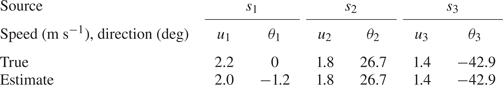
As can be observed, the estimated magnitudes and direction angles of the two TS sources are in excellent agreement with the true values, obtained via LST simulation, whereas the estimates corresponding to the WP source exhibit moderate errors. These estimation errors can be attributed, in part, to our choice to compare the estimates to the WP group velocity, because of its dispersive nature. Another factor that can contribute to the estimation errors is the smoothing resolution of the DUET histogram ($\varDelta _\alpha$ and $\varDelta _\delta$), used in (2.17) to determine the mixing parameters. We tune this resolution so as to bear a negligible impact on the estimates of the magnitude and direction of the velocity vector.

5.1. Experiment 1: blind disturbance separation with two sensors

The set-up of the first experiment is shown in figure 14. An SDBD plasma actuator and a loudspeaker are used to generate two sources introduced upstream of the two hot-wire sensors, creating, in each sensor, a mixture comprising a TS wave and a WP. Specifically, placed outside the test section of the wind tunnel, the loudspeaker generates $s_1$, a single 60 Hz frequency disturbance (TS wave). Mounted on the plate 0.3 m downstream of the leading edge, the SDBD plasma actuator is used to generate $s_2$, a two-dimensional WP, being actuated via a 50 ms pulse signal. The free-stream velocity is set to 4.1 m s$^{-1}$. The sensors are positioned at 0.775 and 0.78 m downstream from the leading edge, with a 40 mm spanwise separation between them. Sensors 1 and 2 are placed at heights that correspond to 0.19$U_\infty$ and 0.23$U_\infty$, respectively (for sensor 2, this value is obtained at $y=0.77$ mm).

Figure 14.

Flow over a flat plate with two disturbance generators: $s_1$ (loudspeaker source) and $s_2$ (plasma actuator source); and two hot-wire sensors: $x_1$ and $x_2$. Experimental set-up sketch.

Figures 15(a) and 15(d) display the streamwise velocity components, measured by two hot-wire sensors, after these signals are conditioned as described in Appendix C. The corresponding Fourier transforms are shown in figures 15(b) and 15(e), and the spectrograms of the mixtures are shown in figures 15(c) and 15(f), respectively. Figures 15(b) and 15(e) demonstrate that the dominant frequencies are, indeed, strongly related to the introduced sources. The bell-shaped signature of the WP has a dominant frequency of about 30 Hz, whereas the second source, generated by the loudspeaker, appears as a single-amplitude peak at 60 Hz. In addition, using a logarithmic scale in figures 15(c) and 15(f) reveals the weak presence of frequencies associated with experimental artifacts and the presence of noise in both mixtures. These were not removed by the signal preprocessing, because of their frequency-domain overlap with the sources comprising the mixture.

Figure 15.

Mixtures as measured by two sensors: (a) $x_1$ and (d) $x_2$. Corresponding Fourier transforms: (b) $E_{x_1}$ and (e) $E_{x_2}$. Corresponding spectrograms (dB), for which a window of 512 ms is used: (c) $|\hat {x}_1|$ and (f) $|\hat {x}_2|$.

Figure 16 shows that the DUET-based method successfully identifies the correct number of introduced sources. The isometric view of the histogram, presented in figure 16(b), shows two peaks associated with two true TS and WP sources. Figure 16(a) displays the peak contours located around a mixing-parameter pair 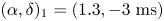$(\alpha ,\delta )_1 = (1.3,-3\ \text {ms})$, whereas the WP peak contours are located at $(\alpha ,\delta )_2=(-0.8,3.5\ \text {ms})$. The estimated delay parameter of the WP source, along with the known sensor downstream position, enable finding the WP envelope velocity: $c_g\approx ({l_{x_1}-l_{x_2}})/{\delta _2}=5/3.5=1.43$ m s$^{-1}$, which is $0.36U$, where $U$ is the free-stream velocity. This result is in agreement with the analysis presented in (Gaster & Grant Reference Gaster and Grant1975), according to which the leading edge of the WP envelope in a BBL propagates at a velocity of $0.44U_\infty$, whereas the trailing edge of the envelope propagates at $0.36U_\infty$.

Figure 16.

A DUET two-dimensional cross power weighted $(p = 1, q = 0)$ histogram of symmetric attenuation $\alpha =(a - 1/a)$ and delay estimate pairs from two mixtures of two sources. (a) Contour plot of the two-dimensional histogram. (b) Isometric view.

Obtained from the histogram peak locations, the identified mixing parameters are used to demix the sources. Figure 17 shows the two estimated sources as identified by the DUET method. Figures 17(a) and 17(d) clearly feature typical TS and WP time signatures, respectively. The noise, which is evident in the spectrograms of the measured mixtures in figure 15, is also evident in the spectrograms of the identified sources in figure 17. Nevertheless, the unique signature of each source is almost uncontaminated by that of the other source, indicating that the DUET method is robust with respect to low noise contamination levels that are hard to avoid in experiments.

Figure 17.

The DUET estimates of sources: (a) $y_1$ and (d) $y_2$. Corresponding Fourier transforms: (b) $E_{y_1}$ and (e) $E_{y_2}$. Corresponding spectrograms (dB): (c) $|\hat {y}_1|$ and (f) $|\hat {y}_2|$.

This experimental example demonstrates that the DUET method performs well as a source identification and separation method, when applied to disturbances acting in a transitional boundary layer. We have obtained similar results in other experiments, under different mixing scenarios.

5.2. Experiment 2: disturbance velocity estimation

This experiment tests the performance of our DUET-based disturbance propagation velocity estimator. The experimental set-up is almost identical to the one described in § 5.1, except that, instead of using a loudspeaker, an additional plasma actuator is used to generate the second source, as depicted in figure 18. The two SDBD plasma actuators are mounted such that one is placed spanwise parallel to the leading edge and located at $x=300$ mm downstream from the plate's leading edge, whereas the other is inclined at $15^\circ$ to the leading edge, and its centre ($z=0$ mm) is located at $x=500$ mm. The inclined actuator can generate oblique TS wave or WP disturbances.

Figure 18.

Experimental set-up of flow over a flat plate equipped with two active plasma actuators. (a) Photo of experimental set-up and (b) schematic diagram of experimental set-up. The region of the hot-wire sensors position is denoted by the magenta square.

The two SDBD actuators are used to introduce two disturbances into the boundary layer. The plasma actuator parallel to the leading edge is used to generate $s_1$, a two-dimensional WP source, travelling downstream at $\theta =0^\circ$ (so that $\beta _0=0$, by (4.15)). The inclined plasma actuator is used to generate $s_2$, an oblique WP source, travelling downstream at $\theta \approx -15^\circ$. Both actuators are driven by a single, 10 ms pulse, such that the actuator parallel to the leading edge is delayed by 10 ms with respect to the other, to render both sources distinguishable in the time–frequency domain. To ensure linear interactions, both actuators are driven by the smallest voltage that still generates uniform discharge along the actuator span.

The free-stream velocity $U_{\infty }$ is set to 5 m s$^{-1}$. All sensors are placed at 0.5 mm height above the plate's surface, rendering a measured mean streamwise velocity of 0.27$U_\infty$ at that height. Three sensor configurations, shown in figure 19 and termed ‘asymmetric’, ‘singular’ and ‘symmetric’, are tested (see Appendix B.4 for the technique used to realize a three-sensor configuration using only two hot wires). In each configuration the sensors are located at the central region of the plate, and the fixed sensor (sensor 1) is placed at $ {\boldsymbol {r}}_{x_1}=[643, \ 25]$ mm. The small variations in sensor pair locations between the configurations, as shown in figure 19, translate to different source arrival times at the sensors.

Figure 19.

Top ($x$–$z$ plane) view of three studied sensor configurations relative to $ {\boldsymbol {r}}_{x_1}=[643,\ 25]$ mm (at the origin). The sensors are denoted by symbols: $\times$, sensor 1 (master); circle, sensor 2 (slave); square, sensor 3 (slave). Baselines are denoted by arrows. (a) Asymmetric configuration, (b) singular configuration and (c) symmetric configuration.

Typical mixtures, measured by sensors 1 and 3 in the asymmetric configuration, are shown in figure 20. The presence of both WP sources is evident in both measured mixtures. The corresponding DUET-estimated sources are shown in figure 21, which demonstrates effective source separation. Similar results, not shown here for conciseness, were obtained for the singular and symmetric sensor configurations.

Figure 20.

Mixtures as measured by two sensors for the asymmetric configuration: (a) $x_1$ and (d) $x_3$. Corresponding Fourier transforms: (b) $E_{x_1}$ and (e) $E_{x_3}$. Corresponding spectrograms (dB), for which a window of 128 ms is used: (c) $|\hat {x}_1|$ and (f) $|\hat {x}_3|$.

Figure 21.

The DUET estimates of sources using sensors 1 and 3 in asymmetric configuration: (a) $y_1$ and (d) $y_2$. Corresponding Fourier transforms: (b) $E_{y_1}$ and (e) $E_{y_2}$. Corresponding spectrograms (dB): (c) $|\hat {y}_1|$ and (f) $|\hat {y}_2|$.

For each of the three sensor configurations, we overlay, in figure 22, the histogram obtained by using sensors 1 and 3 (blue contours) on the histogram obtained by using sensors 1 and 2 (black contours). As can be clearly observed, the black contours are shifted to the right relative to the blue ones, that is, $|\delta _{j13}| < |\delta _{j12}|$, which agrees with the position of sensor 2 being downstream of sensor 3 in all three configurations.

Figure 22.

Top view of DUET two-dimensional cross power weighted ($p = 1$, $q = 0$) histograms for the studied three-sensor configurations. The histogram computed using sensors 1 and 3 (blue contours) is overlaid on the histogram computed using sensors 1 and 2 (black contours). (a) Asymmetric configuration, (b) singular configuration and (c) symmetric configuration.

Next, we use the source delays, estimated from both histograms, to evaluate the corresponding velocity vector magnitude and direction by applying the method of § 3. These estimates are shown graphically in figure 23 and summarized numerically in table 3, for each of the tested sensor configurations.

Figure 23.

Estimated velocities of sources $s_1$ (blue) and $s_2$ (red) using the three studied sensor configurations. (a) Asymmetric configuration, (b) singular configuration and (c) symmetric configuration. The regions of ${\kappa ({\boldsymbol{\mathsf{W}}})}>50$ are denoted by red dots.

Table 3.

Estimated source velocities.

The results show that the streamwise-travelling two-dimensional WP disturbance is estimated quite consistently by all three sensor configurations. The oblique WP estimates, on the other hand, exhibit a substantially larger variation. Nevertheless, the estimated WP envelope velocities of both sources are between $0.3U_{\infty }$ and $0.45U_{\infty }$, which are close to the values of our numerical example (see § 4.6).

The discrepancy of about $3^\circ$ between the estimated $\theta _1$ and the $0^\circ$ angle of the parallel actuator (that created it) can be attributed to several factors: (1) an imperfect alignment of the sensor on the $x$–$z$ plane (the positioning accuracy was 1 mm), (2) random artifacts, caused by the fact that two repeated experiments had to be done to obtain the required three sensor measurements with only two sensors, (3) DUET histogram resolution (although this resolution was tuned to bear a negligible impact on the estimates of the velocity vector), (4) the disturbance can, potentially, not precisely adhere to the inclination angle of its generating actuator when propagating downstream and (5) slight variations in the phase profiles may exist, in particular for the $s_1$ WP. In what follows, we examine the latter two factors in further detail.

To investigate how the generated disturbance changes its inclination angle as it propagates downstream from its generating actuator, we track the temporal evolution of a localized disturbance within the boundary layer over a flat plate. Figure 24 shows the time history of the streamwise velocity of the disturbances as they pass through two points, located at 600 and 650 mm from the leading edge, both at a height of $y=0.9$ mm above the plate. Consisting of $10^3$ points, the velocity record is digitized at 1 kHz, such that the total measuring time is 1 s for each $(x,y,z)$ location. The measurement sequence is synchronized by a pulse from the computer that triggers the disturbance generator. The inclined actuator, which generates $s_2$, and the parallel actuator, which generates $s_1$, are triggered 0.2 and 0.5 s after the beginning of the recording, respectively. At each measuring point, an ensemble average of six realizations of the disturbance passage is computed (this number of realizations was found to be sufficient to adequately represent the flow structure).

Figure 24.

Time histories of streamwise disturbance velocity at two downstream stations. (a) Colourbar for (b,c). Time history of streamwise disturbance velocity at (b) $y=0.9$ mm, $x=600$ mm and (c) $y=0.9$ mm, $x=650$ mm. (d) Pulsation sequence of actuator parallel to leading edge (blue) and inclined actuator (red). Free-stream velocity is $U=5$ m s$^{-1}$. In (b,c) the estimated values of WP envelope inclination angles are denoted by the red ($s_2$) and blue ($s_1$) lines.

In figure 24 the WP propagation angle at both measuring points is evident within the central region, where the boundary layer maintains its laminarity and is not affected by the spanwise edges of the plate. Assuming that the propagation angles remain fixed from disturbance generation until the mixtures reach the sensors, we use the estimated angles from table 3 to plot the estimated wavefront inclination angle in the $t$–$z$ domain over the measured time history of the flow. As figure 24 clearly shows, the inclined WP source, $s_2$, is estimated very well, and better than the WP source $s_1$. This is most likely due to the phase changes of $s_1$ at the sampled locations.

To determine if there are slight variations in the disturbance phase profiles, we plot in figure 25(a) the same time histories used to obtain figure 24(c), on the $t$–$y$ domain, at $x=600$ mm and $z = 0$ mm. The free-stream velocity is $U=5$ m s$^{-1}$. The signals are normalized by their maximal values to make them more pronounced. In figure 25(b) we show the mean profile of the flow without actuation at the same location, in order to reference the sensor heights to the canonical boundary layer at that location. Some slight non-coherence in the shape of source $s_1$ is evident below the height of 1 mm (which is below 0.35$U_\infty$), indicating disturbance phase variations at that region. Thus, placing sensors at that height reduces our method's precision in estimating the velocity vector of source $s_1$.

Figure 25.

(a) Time history of disturbance streamwise velocity on the $t$–$y$ domain and (b) mean flow profile without actuation, both obtained at $x=600$ mm and $z=0$ mm, for $U_\infty =5$ m s$^{-1}$.