





1. Introduction
Boundary layer transition through deterministic input actuation has been extensively studied to understand fundamental mechanisms underlying the path to turbulence. Fasel, Rist & Konzelmann (Reference Fasel, Rist and Konzelmann1990) and Rist & Fasel (Reference Rist and Fasel1995) conducted seminal direct numerical simulation (DNS) of controlled K-type transition in flat-plate boundary layers, successfully reproducing wind tunnel experiments by Klebanoff, Tidstrom & Sargent (Reference Klebanoff, Tidstrom and Sargent1962), Kachanov, Kozlov & Levchenko (Reference Kachanov, Kozlov and Levchenko1977) and Kachanov & Levchenko (Reference Kachanov and Levchenko1984). Bake, Meyer & Rist (Reference Bake, Meyer and Rist2002) studied, through a comparison of DNS and experiments, the complex flow randomisation process that transforms small disturbances into developed boundary layer turbulence, providing local phenomenological insights into the breakdown of organised structures. Sayadi, Hamman & Moin (Reference Sayadi, Hamman and Moin2013) demonstrated that complete K- and H-type transitions converge towards fully developed turbulence after the skin-friction overshoot, revealing that initially periodic ‘hairpin packets’ eventually produce statistical properties of fully developed turbulence. Towards the stability analysis of canonical transition, Herbert (Reference Herbert1988) established a framework for analysing secondary instability mechanisms in the K- and H-type transition scenarios. Monokrousos et al. (Reference Monokrousos, Akervik, Brandt and Henningson2010) identified optimal forcing mechanisms and initial conditions for instability growth in the Blasius boundary layer, while Cherubini et al. (Reference Cherubini, De Palma, Robinet and Bottaro2011) investigated optimal perturbations and minimal seeds using time-domain optimisation approaches. Rigas, Sipp & Colonius (Reference Rigas, Sipp and Colonius2021) extended input $/$
output analysis to account for nonlinear triadic interactions via harmonic balance models, solving transition scenarios up to before the skin friction maximum (
$/$
output analysis to account for nonlinear triadic interactions via harmonic balance models, solving transition scenarios up to before the skin friction maximum ( $C_f^{\textit{max}}$
) within the frequency domain.
$C_f^{\textit{max}}$
) within the frequency domain.
Regimes of the transition process. (a) Instantaneous snapshot of full DNS data $\boldsymbol{q}$
. (b) Fundamental harmonic response
$\boldsymbol{q}$
. (b) Fundamental harmonic response $\tilde {\boldsymbol{q}}$
. (c) Cyclo-stationary fluctuation
$\tilde {\boldsymbol{q}}$
. (c) Cyclo-stationary fluctuation $\boldsymbol{q}''\!=\boldsymbol{q} \!-\tilde {\boldsymbol{q}}$
. (d) Symmetric
$\boldsymbol{q}''\!=\boldsymbol{q} \!-\tilde {\boldsymbol{q}}$
. (d) Symmetric $\boldsymbol{q}^s$
and anti-symmetric
$\boldsymbol{q}^s$
and anti-symmetric $\boldsymbol{q}^a$
components of temporal and spatial symmetry breaking (
$\boldsymbol{q}^a$
components of temporal and spatial symmetry breaking ( $\boldsymbol{q}'' \!=\boldsymbol{q}^s \!+\boldsymbol{q}^a$
).
$\boldsymbol{q}'' \!=\boldsymbol{q}^s \!+\boldsymbol{q}^a$
). $Q$
-criterion isosurfaces (all
$Q$
-criterion isosurfaces (all $Q=10^3$
); coloured in the respective
$Q=10^3$
); coloured in the respective $u$
-velocities (
$u$
-velocities ( $w$
-velocity for
$w$
-velocity for $\boldsymbol{q}^a$
). (e) Regimes labelled on the
$\boldsymbol{q}^a$
). (e) Regimes labelled on the $C_f$
graph. See supplementary movie 1 available at https://doi.org/10.1017/jfm.2026.11423.
$C_f$
graph. See supplementary movie 1 available at https://doi.org/10.1017/jfm.2026.11423.

Modal analysis has been a valuable tool for identifying coherent structures in transitional flows. Rempfer & Fasel (Reference Rempfer and Fasel1994a , Reference Rempfer and Faselb ) pioneered the application of proper orthogonal decomposition (POD) (Sirovich Reference Sirovich1987a ; Aubry Reference Aubry1991) to identify three-dimensional coherent structures and their dynamics in K-type transition. Recent advances in modal decomposition include spectral POD (Lumley Reference Lumley1970; Towne, Schmidt & Colonius Reference Towne, Schmidt and Colonius2018) for extracting frequency domain modes and space–time POD (Schmidt & Schmid Reference Schmidt and Schmid2019; Frame & Towne Reference Frame and Towne2023) for general spatio-temporal modes without imposing assumptions on time dynamics. Both methods have been applied to data from fully turbulent boundary layers (Tutkun & George Reference Tutkun and George2017; Hack & Schmidt Reference Hack and Schmidt2021). Heidt & Colonius (Reference Heidt and Colonius2024) extended SPOD to harmonically forced flows, assuming a frequency domain ansatz with specific periodic modal forms.
Despite these advances, the specific mechanisms driving the breaking of temporal (periodicity) and spatial (spanwise) symmetries, the hallmark phenomena of chaos and turbulence in deterministic transition, remain unclear. While the roots of aperiodicity $/$
asymmetry are small disturbances (of numerical or physical nature) in time
$/$
asymmetry are small disturbances (of numerical or physical nature) in time $/$
space, to which the flow is inherently sensitive, the resulting transition manifests via energetically interacting coherent structures. In figure 1, we provide an overview of the streamwise development of flow dynamics and symmetries. The initially periodic and symmetric flow departs from the laminar solution, and undergoes temporal and spatial symmetry breaking, marked by increasing non-periodicity and asymmetry, as it progresses through the
$/$
space, to which the flow is inherently sensitive, the resulting transition manifests via energetically interacting coherent structures. In figure 1, we provide an overview of the streamwise development of flow dynamics and symmetries. The initially periodic and symmetric flow departs from the laminar solution, and undergoes temporal and spatial symmetry breaking, marked by increasing non-periodicity and asymmetry, as it progresses through the $C_f^{\textit{max}}$
. Afterwards, the cyclo-stationary state converges to statistical stationarity as the statistics asymptotically collapse onto turbulent correlations (White Reference White2006). Throughout our analysis, we track the evolution from deterministic periodic states to quasi-periodic and broadband dynamics, and characterise a variety of coherent structures for these specific regimes. We demonstrate that both temporal and spatial symmetry breaking are identifiable as organised, energetically dominant modes with distinct dynamical properties. Finally, by analysing their energy transfer budgets, we reveal that these modes act as a conduit, directing energy from deterministic to broadband dynamics.
$C_f^{\textit{max}}$
. Afterwards, the cyclo-stationary state converges to statistical stationarity as the statistics asymptotically collapse onto turbulent correlations (White Reference White2006). Throughout our analysis, we track the evolution from deterministic periodic states to quasi-periodic and broadband dynamics, and characterise a variety of coherent structures for these specific regimes. We demonstrate that both temporal and spatial symmetry breaking are identifiable as organised, energetically dominant modes with distinct dynamical properties. Finally, by analysing their energy transfer budgets, we reveal that these modes act as a conduit, directing energy from deterministic to broadband dynamics.
2. Methods
We compute the DNS of K-type transition with the CharLES solver on a structured mesh, satisfying $y^+ \lt 1$
across the entire Reynolds number range from
$y^+ \lt 1$
across the entire Reynolds number range from ${\textit{Re}}_x = 1 \times 10^5$
to
${\textit{Re}}_x = 1 \times 10^5$
to $6.5 \times 10^5$
. Transition is triggered by a forcing strip that introduces a periodic (
$6.5 \times 10^5$
. Transition is triggered by a forcing strip that introduces a periodic ( $f_1 = 8.75$
) Tollmien–Schlichting (TS) wave with a weak symmetric peak (
$f_1 = 8.75$
) Tollmien–Schlichting (TS) wave with a weak symmetric peak ( $f_0 = 0$
). For details on the numerics and validation, we refer the reader to Lin & Schmidt (Reference Lin and Schmidt2024). To converge the dominant modes, we sample a dataset of 198 forcing periods (
$f_0 = 0$
). For details on the numerics and validation, we refer the reader to Lin & Schmidt (Reference Lin and Schmidt2024). To converge the dominant modes, we sample a dataset of 198 forcing periods ( $T_1=1/f_1$
) with 128 DNS snapshots each.
$T_1=1/f_1$
) with 128 DNS snapshots each.
2.1. Spatio-temporal symmetry decomposition
To study the transition process through the lens of spatial and temporal symmetry breaking, we introduce the following decomposition of the flow field:
 \begin{align} \boldsymbol{q}({\boldsymbol{x}}, t) &=\, \underbrace {\boldsymbol{q}^S({\boldsymbol{x}}, t)}_{\textrm {symmetric}} \,+\, \underbrace {\boldsymbol{q}^A({\boldsymbol{x}}, t)}_{\textrm {anti-symmetric}} = \underbrace {\tilde {\boldsymbol{q}}({\boldsymbol{x}}, t)}_{\textrm {harmonics (FHR)}} \, +\, \overbrace { \underbrace {\boldsymbol{q}^s({\boldsymbol{x}}, t)}_{\textrm {sym. fluctuation}} \,+\, \underbrace {\boldsymbol{q}^a({\boldsymbol{x}}, t)}_{\textrm {anti-sym. fluctuation}} } ^{{\textrm {cyclo-stat. fluctuation }} \boldsymbol{q}''}\nonumber\\ &=\, \underbrace {\tilde {\boldsymbol{q}}({\boldsymbol{x}}, t)}_{\textrm {sym. periodic}} \,+\, \underbrace {\boldsymbol{q}^{\bullet }({\boldsymbol{x}}, t)}_{\textrm {sym. quasi-periodic}} \,+\, \underbrace {\boldsymbol{q}^{\circ }({\boldsymbol{x}}, t)}_{\textrm {sym. broadband}} \, + \, \underbrace {\boldsymbol{q}^{{\blacktriangle }}({\boldsymbol{x}}, t)}_{\textrm {anti-sym. quasi-periodic}}\, +\, \underbrace {\boldsymbol{q}^{{\vartriangle }}({\boldsymbol{x}}, t)}_{\textrm {anti-sym. broadband}}. \end{align}
Here, the superscripts encode spatial symmetry, while the symbols $\{\bullet /{\blacktriangle } , \circ /{\vartriangle }\}$
distinguish quasi-periodic mode dynamics from broadband (aperiodic) residual dynamics. The
$\{\bullet /{\blacktriangle } , \circ /{\vartriangle }\}$
distinguish quasi-periodic mode dynamics from broadband (aperiodic) residual dynamics. The $S/A$
components in the first line of (2.1) are obtained by the transverse
$S/A$
components in the first line of (2.1) are obtained by the transverse $D_1$
(dihedral group 1) symmetry decomposition (Sirovich Reference Sirovich1987b
) about the
$D_1$
(dihedral group 1) symmetry decomposition (Sirovich Reference Sirovich1987b
) about the $z=0$
midplane as
$z=0$
midplane as
 \begin{equation} \boldsymbol{q}^{S/A}(x, y, z ,t) = \frac {1}{2} \left [\!\! \begin{array}{c} u(x, y, z ,t) \pm u(x, y, -z ,t) \\ v(x, y, z ,t) \pm v(x, y, -z ,t) \\ w(x, y, z ,t) \mp w(x, y, -z ,t) \end{array}\!\!\right ]\!, \end{equation}
with the top (bottom) signs yielding $\boldsymbol{q}^S$
(
$\boldsymbol{q}^S$
( $\boldsymbol{q}^A$
). By contrast, separating periodic, quasi-periodic and stochastic contributions in the second line of (2.1) requires the modal decompositions introduced in the following. For the K-type transition scenario, the deterministic fundamental harmonic response (FHR) is symmetric and periodic. Furthermore, the FHR persists under phase-averaging as it is composed exclusively of harmonics that are
$\boldsymbol{q}^A$
). By contrast, separating periodic, quasi-periodic and stochastic contributions in the second line of (2.1) requires the modal decompositions introduced in the following. For the K-type transition scenario, the deterministic fundamental harmonic response (FHR) is symmetric and periodic. Furthermore, the FHR persists under phase-averaging as it is composed exclusively of harmonics that are $T_1$
-periodic. The anti-symmetric class contains no deterministic component and is thus purely fluctuating, implying
$T_1$
-periodic. The anti-symmetric class contains no deterministic component and is thus purely fluctuating, implying $\boldsymbol{q}^A=\boldsymbol{q}^a$
.
$\boldsymbol{q}^A=\boldsymbol{q}^a$
.
2.2. Spectral proper orthogonal decomposition (SPOD)
SPOD identifies frequency-specific, time-periodic coherent structures $\boldsymbol{\psi}(\boldsymbol{x},f)$
in statistically stationary flows (Lumley Reference Lumley1970; Towne et al. Reference Towne, Schmidt and Colonius2018; Schmidt & Colonius Reference Schmidt and Colonius2020). Here, the space–time correlation tensor
$\boldsymbol{\psi}(\boldsymbol{x},f)$
in statistically stationary flows (Lumley Reference Lumley1970; Towne et al. Reference Towne, Schmidt and Colonius2018; Schmidt & Colonius Reference Schmidt and Colonius2020). Here, the space–time correlation tensor $\boldsymbol{C}(\boldsymbol{x},\boldsymbol{x}',\tau )$
(where
$\boldsymbol{C}(\boldsymbol{x},\boldsymbol{x}',\tau )$
(where $\tau =t-t'$
) is Fourier-transformed to the cross-spectral density (CSD) tensor
$\tau =t-t'$
) is Fourier-transformed to the cross-spectral density (CSD) tensor $\boldsymbol{S}(\boldsymbol{x}, \boldsymbol{x}', f) = \int _{-\infty }^{\infty } \boldsymbol{C}(\boldsymbol{x}, \boldsymbol{x}', \tau ) e^{\textrm{i} 2 \pi f \tau} \,{\mathrm{d}}\tau$
to solve the respective continuous and discrete eigenvalue problems
$\boldsymbol{S}(\boldsymbol{x}, \boldsymbol{x}', f) = \int _{-\infty }^{\infty } \boldsymbol{C}(\boldsymbol{x}, \boldsymbol{x}', \tau ) e^{\textrm{i} 2 \pi f \tau} \,{\mathrm{d}}\tau$
to solve the respective continuous and discrete eigenvalue problems
 \begin{align} \int _{V} \boldsymbol{S}(\boldsymbol{x},\boldsymbol{x}', f) \boldsymbol{W}(\boldsymbol{x}') \boldsymbol{\psi}(\boldsymbol{x}', f) \, {\mathrm{d}}\boldsymbol{x}' &= \lambda (f) \boldsymbol{\psi}(\boldsymbol{x}, f), \end{align}
 \begin{align} {1}/{N_b} \hspace {2pt} \hat {\mathbf{Q}}_{k}\hat {\mathbf{Q}}_{k}^*{\mathbf{W}}\boldsymbol{\Psi}_{k} &= \boldsymbol{\Psi}_{k}\boldsymbol{\Lambda }_{k}, \end{align}
where $\hat {\mathbf{Q}}_{k}$
stores different realisations of the Fourier modes
$\hat {\mathbf{Q}}_{k}$
stores different realisations of the Fourier modes $\hat {\mathbf{q}}_{k}({\mathbf{x}})$
at frequency
$\hat {\mathbf{q}}_{k}({\mathbf{x}})$
at frequency $f_k$
and the CSD is estimated as
$f_k$
and the CSD is estimated as ${\mathbf{S}}_k=E_b\{\hat {\mathbf{q}}_{k}({\mathbf{x}})\hat {\mathbf{q}}^*_{k}({\mathbf{x}}) \}$
with block-wise expectation
${\mathbf{S}}_k=E_b\{\hat {\mathbf{q}}_{k}({\mathbf{x}})\hat {\mathbf{q}}^*_{k}({\mathbf{x}}) \}$
with block-wise expectation $E_b\{\boldsymbol{\cdot }\}$
(Welch Reference Welch1967). The columns of
$E_b\{\boldsymbol{\cdot }\}$
(Welch Reference Welch1967). The columns of $\boldsymbol{\Psi }_{k}$
are discrete SPOD modes
$\boldsymbol{\Psi }_{k}$
are discrete SPOD modes $\boldsymbol{\unicode{x03C8}}_{k}^{(m)}({{\mathbf{x}}})$
and
$\boldsymbol{\unicode{x03C8}}_{k}^{(m)}({{\mathbf{x}}})$
and $\boldsymbol{\Lambda }_{k}=\text{diag}(\boldsymbol{\unicode{x03BB}}_{k})$
stores their energies
$\boldsymbol{\Lambda }_{k}=\text{diag}(\boldsymbol{\unicode{x03BB}}_{k})$
stores their energies $\lambda_{k}^{(m)}$
. Expansion coefficients are recovered in the rows of
$\lambda_{k}^{(m)}$
. Expansion coefficients are recovered in the rows of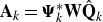 ${{\mathbf{A}}}_{k} = \boldsymbol{\Psi }_{k}^*{\mathbf{W}}\hat {\mathbf{Q}}_{k}$
, with
${{\mathbf{A}}}_{k} = \boldsymbol{\Psi }_{k}^*{\mathbf{W}}\hat {\mathbf{Q}}_{k}$
, with ${{\mathbf{A}}}_{k}^*{{\mathbf{A}}}_{k} = \boldsymbol{\Lambda }_{k}$
. SPOD modes are single-frequency oscillatory coherent structures that optimally capture the variance of the data at that frequency and are orthonormal in the space– and infinite-time norm
${{\mathbf{A}}}_{k}^*{{\mathbf{A}}}_{k} = \boldsymbol{\Lambda }_{k}$
. SPOD modes are single-frequency oscillatory coherent structures that optimally capture the variance of the data at that frequency and are orthonormal in the space– and infinite-time norm $\langle \boldsymbol{\cdot }, \boldsymbol{\cdot }\rangle _{\boldsymbol{x},t}$
. They are thus statistically optimal linear combinations of Fourier modes.
$\langle \boldsymbol{\cdot }, \boldsymbol{\cdot }\rangle _{\boldsymbol{x},t}$
. They are thus statistically optimal linear combinations of Fourier modes.
2.3. Space–time proper orthogonal decomposition (STPOD)
STPOD extracts space–time energy-optimal spatio-temporal modes $\boldsymbol{\phi}(\boldsymbol{x},t)$
over a finite time window
$\boldsymbol{\phi}(\boldsymbol{x},t)$
over a finite time window $\Delta T$
, chosen here as one actuation period
$\Delta T$
, chosen here as one actuation period $T_1$
. The modes solve the respective continuous and discrete eigenvalue problems (Lumley Reference Lumley1970; Schmidt & Schmid Reference Schmidt and Schmid2019)
$T_1$
. The modes solve the respective continuous and discrete eigenvalue problems (Lumley Reference Lumley1970; Schmidt & Schmid Reference Schmidt and Schmid2019)
 \begin{align} \int _{\Delta T} \int _V \boldsymbol{C}(\boldsymbol{x},\boldsymbol{x}',t,t') \boldsymbol{W}(\boldsymbol{x}') \boldsymbol{\phi}(\boldsymbol{x}', t') \, {\mathrm{d}}\boldsymbol{x}' \, {\mathrm{d}}t' &= \lambda \boldsymbol{\phi}(\boldsymbol{x}, t), \end{align}
 \begin{align} {1}/{N_{j}} \hspace {2pt} {\mathbf{Q}}{\mathbf{Q}}^*{\mathbf{W}}\boldsymbol{\Phi } &= \boldsymbol{\Phi }\boldsymbol{\Lambda }, \end{align}
over a spatial domain $V$
, with positive-definite weight matrix
$V$
, with positive-definite weight matrix $\boldsymbol{W}(\boldsymbol{x})$
and statistically estimated two-point space–time correlation tensor
$\boldsymbol{W}(\boldsymbol{x})$
and statistically estimated two-point space–time correlation tensor $\boldsymbol{C}(\boldsymbol{x},\boldsymbol{x}',t,t')=E\{\boldsymbol{q}(\boldsymbol{x}, t)\boldsymbol{q}^*(\boldsymbol{x}', t') \}$
. The modes
$\boldsymbol{C}(\boldsymbol{x},\boldsymbol{x}',t,t')=E\{\boldsymbol{q}(\boldsymbol{x}, t)\boldsymbol{q}^*(\boldsymbol{x}', t') \}$
. The modes $\boldsymbol{\phi}(\boldsymbol{x},t)$
are orthonormal in the space– and finite-time norm
$\boldsymbol{\phi}(\boldsymbol{x},t)$
are orthonormal in the space– and finite-time norm $\langle \boldsymbol{\cdot }, \boldsymbol{\cdot }\rangle _{\boldsymbol{x},\Delta T}$
. For the discrete problem, snapshots of
$\langle \boldsymbol{\cdot }, \boldsymbol{\cdot }\rangle _{\boldsymbol{x},\Delta T}$
. For the discrete problem, snapshots of ${\mathbf{q}}({{\mathbf{x}}}, t)$
are stacked column-wise over
${\mathbf{q}}({{\mathbf{x}}}, t)$
are stacked column-wise over $\Delta T$
for each realisation
$\Delta T$
for each realisation $j$
, and different realisations are concatenated row-wise to form the data matrix
$j$
, and different realisations are concatenated row-wise to form the data matrix ${\mathbf{Q}}$
, which is then decomposed by (2.6). The discrete STPOD modes
${\mathbf{Q}}$
, which is then decomposed by (2.6). The discrete STPOD modes $\boldsymbol{\unicode{x03D5}}_m({{\mathbf{x}}},t)$
form the columns of
$\boldsymbol{\unicode{x03D5}}_m({{\mathbf{x}}},t)$
form the columns of $\boldsymbol{\Phi }$
and
$\boldsymbol{\Phi }$
and $\boldsymbol{\Lambda }=\text{diag}(\boldsymbol{\unicode{x03BB}})$
stores their energies
$\boldsymbol{\Lambda }=\text{diag}(\boldsymbol{\unicode{x03BB}})$
stores their energies $\lambda_m$
. Realisation-varying expansion coefficients
$\lambda_m$
. Realisation-varying expansion coefficients $a_{m,j}$
are obtained as the rows of
$a_{m,j}$
are obtained as the rows of ${{\mathbf{A}}} = \boldsymbol{\Phi }^*{\mathbf{W}}{\mathbf{Q}}$
, with
${{\mathbf{A}}} = \boldsymbol{\Phi }^*{\mathbf{W}}{\mathbf{Q}}$
, with ${{\mathbf{A}}}^*{{\mathbf{A}}} = \boldsymbol{\Lambda }$
. Notably, STPOD specialises to space-only POD in the limit
${{\mathbf{A}}}^*{{\mathbf{A}}} = \boldsymbol{\Lambda }$
. Notably, STPOD specialises to space-only POD in the limit $\Delta T \to 0$
and, assuming statistical stationarity, converges to SPOD in the limit
$\Delta T \to 0$
and, assuming statistical stationarity, converges to SPOD in the limit $\Delta T \to \infty$
(Frame & Towne Reference Frame and Towne2023). Here, STPOD is the most unbiased method with no assumptions about the dynamics of the space–time signal
$\Delta T \to \infty$
(Frame & Towne Reference Frame and Towne2023). Here, STPOD is the most unbiased method with no assumptions about the dynamics of the space–time signal ${\mathbf{q}}({{\mathbf{x}}}, t)$
. Unlike spectral approaches that impose periodicity by default, it produces periodic modes only when they are energetically dominant within a given window
${\mathbf{q}}({{\mathbf{x}}}, t)$
. Unlike spectral approaches that impose periodicity by default, it produces periodic modes only when they are energetically dominant within a given window $\Delta T=T_1$
– a crucial property for symmetry breaking analysis.
$\Delta T=T_1$
– a crucial property for symmetry breaking analysis.
3. Extracting the resonant fundamental harmonic response (FHR)
As we are actuating the eigenmode (TS wave) of a system with quadratic nonlinearities, a resonant response with harmonics must be expected. To extract those harmonic coherent structures, we apply SPOD to the symmetric ( ${\mathbf{q}}^S$
) and anti-symmetric (
${\mathbf{q}}^S$
) and anti-symmetric ( ${\mathbf{q}}^A$
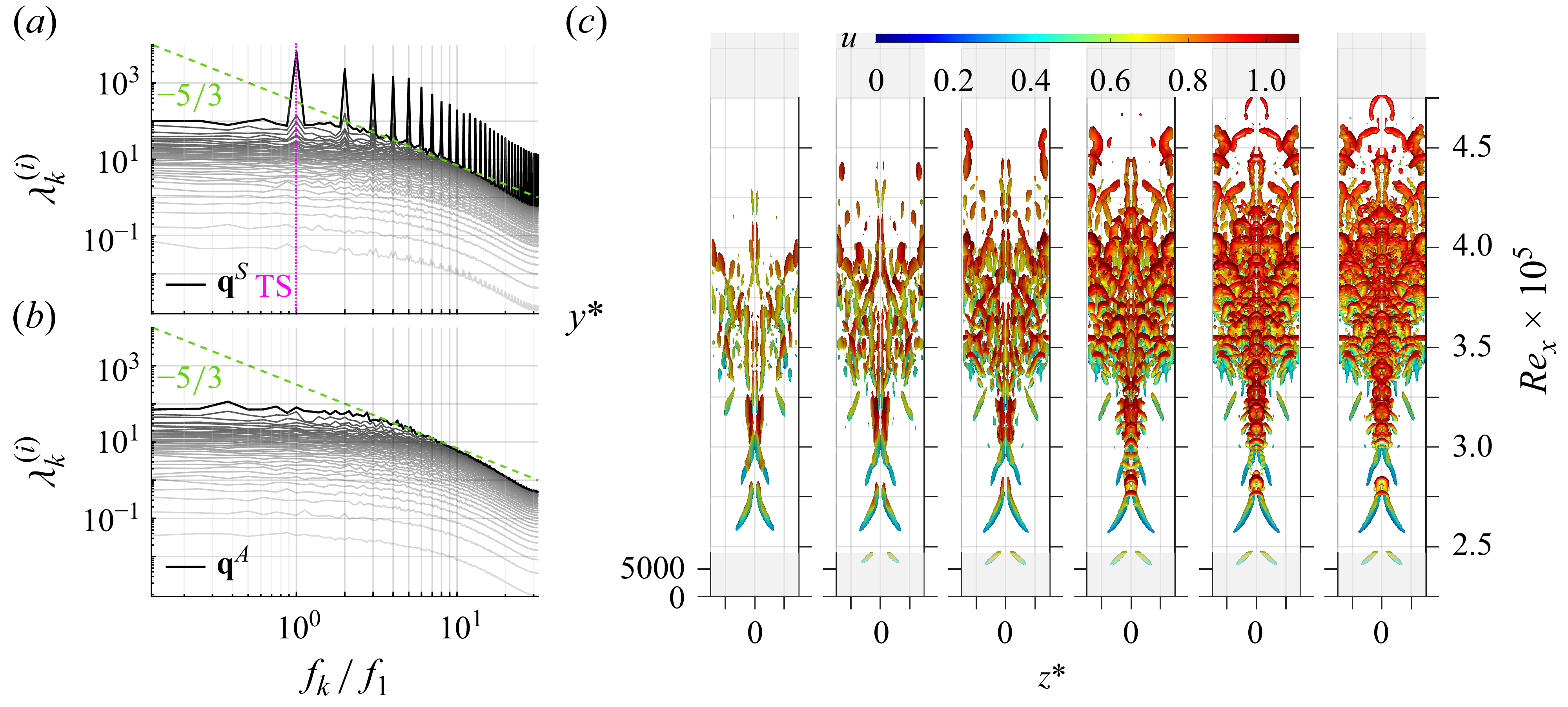
) components individually, yielding energy-optimal modes at each frequency in each symmetry class. Figure 2(a,b) contrasts the
${\mathbf{q}}^A$
) components individually, yielding energy-optimal modes at each frequency in each symmetry class. Figure 2(a,b) contrasts the ${\mathbf{q}}^S$
and
${\mathbf{q}}^S$
and ${\mathbf{q}}^A$
spectra. The
${\mathbf{q}}^A$
spectra. The ${\mathbf{q}}^S$
spectrum is dominated by low-rank peaks at the TS frequency (
${\mathbf{q}}^S$
spectrum is dominated by low-rank peaks at the TS frequency ( $f_k/f_1=1$
) and its harmonics, characteristic of dominant coherent structures, while the noise-like
$f_k/f_1=1$
) and its harmonics, characteristic of dominant coherent structures, while the noise-like ${\mathbf{q}}^A$
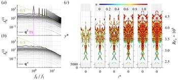
spectrum is broadband with slow rank decay, showing no energetically preferred modes. Thus, the FHR is symmetric, time-periodic and represents the expected deterministic result from symmetric, periodic actuation of the Navier–Stokes equations, as predicted by classical frameworks like harmonic balance (Rigas et al. Reference Rigas, Sipp and Colonius2021). The FHR can be assembled by a linear combination of the first symmetric SPOD modes
${\mathbf{q}}^A$
spectrum is broadband with slow rank decay, showing no energetically preferred modes. Thus, the FHR is symmetric, time-periodic and represents the expected deterministic result from symmetric, periodic actuation of the Navier–Stokes equations, as predicted by classical frameworks like harmonic balance (Rigas et al. Reference Rigas, Sipp and Colonius2021). The FHR can be assembled by a linear combination of the first symmetric SPOD modes $\boldsymbol{\unicode{x03C8}}^{(1)}_{k}$
of the harmonic peaks
$\boldsymbol{\unicode{x03C8}}^{(1)}_{k}$
of the harmonic peaks $f_k=f_n$
(
$f_k=f_n$
( $n \in \mathbb{Z}$
) in figure 2(a):
$n \in \mathbb{Z}$
) in figure 2(a):
 \begin{equation} \tilde {\mathbf{q}}({{\mathbf{x}}},t) \equiv \sum _{n} \boldsymbol{\unicode{x03C8}}^{(1)}_{n} a^{(1)}_{n} e^{(\mathrm{i}2\pi f_n t)} + \bar {\mathbf{q}}({{\mathbf{x}}}) = \tilde {\mathbf{q}}_{\setminus 0}({{\mathbf{x}}}, t) + \bar {\mathbf{q}}({{\mathbf{x}}}), \end{equation}
with the time-averaged mean flow $\bar {\mathbf{q}}({{\mathbf{x}}})$
, and the block-wise estimated dominant SPOD expansion coefficients
$\bar {\mathbf{q}}({{\mathbf{x}}})$
, and the block-wise estimated dominant SPOD expansion coefficients $a^{(1)}_{n}$
. We compute the SPOD using
$a^{(1)}_{n}$
. We compute the SPOD using $N_{\textit{FFT}} = 512$
, eight periods per block and 50 % block overlap. Most notably, figure 2(c) shows that
$N_{\textit{FFT}} = 512$
, eight periods per block and 50 % block overlap. Most notably, figure 2(c) shows that $\tilde {\mathbf{q}}({{\mathbf{x}}},t)$
exhibits compact spatial support when fully assembled and, while the resulting vortical structures closely resemble hairpin ‘packets’ or ‘forests’ in their late stages (often characterised as ‘chaotic’ in the turbulence literature (Adrian Reference Adrian2007; Wu & Moin Reference Wu and Moin2009)), we show that such seemingly disordered structures in fact arise deterministically here as the system’s resonant FHR to periodic actuation of its eigenmode.
$\tilde {\mathbf{q}}({{\mathbf{x}}},t)$
exhibits compact spatial support when fully assembled and, while the resulting vortical structures closely resemble hairpin ‘packets’ or ‘forests’ in their late stages (often characterised as ‘chaotic’ in the turbulence literature (Adrian Reference Adrian2007; Wu & Moin Reference Wu and Moin2009)), we show that such seemingly disordered structures in fact arise deterministically here as the system’s resonant FHR to periodic actuation of its eigenmode.
As illustrated in figure 1 and § 2.1, subtracting the deterministic FHR from the full data yields a turbulent, cyclo-stationary fluctuation ${\mathbf{q}}^{\prime\prime} \equiv {\mathbf{q}} - \tilde {\mathbf{q}}$
. Further splitting this fluctuation into symmetry classes,
${\mathbf{q}}^{\prime\prime} \equiv {\mathbf{q}} - \tilde {\mathbf{q}}$
. Further splitting this fluctuation into symmetry classes, ${\mathbf{q}}'' = {\mathbf{q}}^s + {\mathbf{q}}^a$
, isolates the data components of temporal and spatial symmetry breaking by construction. As
${\mathbf{q}}'' = {\mathbf{q}}^s + {\mathbf{q}}^a$
, isolates the data components of temporal and spatial symmetry breaking by construction. As $\tilde {\mathbf{q}}$
is symmetric and periodic,
$\tilde {\mathbf{q}}$
is symmetric and periodic, ${\mathbf{q}}^s$
must contain all non-periodic symmetric fluctuations that break time symmetry, while any indication of
${\mathbf{q}}^s$
must contain all non-periodic symmetric fluctuations that break time symmetry, while any indication of ${\mathbf{q}}^a$
captures the onset of spanwise asymmetry. This results in a pivotal multiscale separation. We later show in figure 4(c) that the rapid surge of
${\mathbf{q}}^a$
captures the onset of spanwise asymmetry. This results in a pivotal multiscale separation. We later show in figure 4(c) that the rapid surge of ${\mathbf{q}}^s$
and
${\mathbf{q}}^s$
and ${\mathbf{q}}^a$
occurs with a simultaneous decline in the
${\mathbf{q}}^a$
occurs with a simultaneous decline in the $\tilde {\mathbf{q}}$
amplitude, allowing us to locate exactly where symmetry breaking arises.
$\tilde {\mathbf{q}}$
amplitude, allowing us to locate exactly where symmetry breaking arises.
SPOD energy spectra for (a) ${\mathbf{q}}^S$
symmetric and (b)
${\mathbf{q}}^S$
symmetric and (b) ${\mathbf{q}}^A$
anti-symmetric components; compare with Sayadi et al. (Reference Sayadi, Hamman and Moin2013). (c) Superposition of
${\mathbf{q}}^A$
anti-symmetric components; compare with Sayadi et al. (Reference Sayadi, Hamman and Moin2013). (c) Superposition of $N_n$
= {1, 2, 4, 8, 16, 32} dominant SPOD modes
$N_n$
= {1, 2, 4, 8, 16, 32} dominant SPOD modes $\boldsymbol{\unicode{x03C8}}^{(1)}_{n}$
at harmonic peaks
$\boldsymbol{\unicode{x03C8}}^{(1)}_{n}$
at harmonic peaks $f_n$
(3.1);
$f_n$
(3.1); $Q$
-criterion (
$Q$
-criterion ( $Q=10^3$
) coloured by
$Q=10^3$
) coloured by $u$
.
$u$
.
Local power spectral densities of different quantities as a streamwise function of ${\textit{Re}}_x$
, coloured by the ratio of the dominant local SPOD energy over the full local energy
${\textit{Re}}_x$
, coloured by the ratio of the dominant local SPOD energy over the full local energy $\lambda^{(1)}(x)/\sum _i \lambda^{(i)}(x)$
. (a)
$\lambda^{(1)}(x)/\sum _i \lambda^{(i)}(x)$
. (a) ${\mathbf{q}}^S$
full symmetric data. (b)
${\mathbf{q}}^S$
full symmetric data. (b) ${\mathbf{q}}^s$
symmetric fluctuation. (c) Zoom on amplified region, progressive ablation of STPOD modes from
${\mathbf{q}}^s$
symmetric fluctuation. (c) Zoom on amplified region, progressive ablation of STPOD modes from ${\mathbf{q}}^s$
: first two modes (i.e.
${\mathbf{q}}^s$
: first two modes (i.e. ${\mathbf{q}}^{\bullet }$
; resulting in
${\mathbf{q}}^{\bullet }$
; resulting in ${\mathbf{q}}^{s}-{\mathbf{q}}^{\bullet }={\mathbf{q}}^{\circ }$
symmetric residual) versus eight modes subtracted.
${\mathbf{q}}^{s}-{\mathbf{q}}^{\bullet }={\mathbf{q}}^{\circ }$
symmetric residual) versus eight modes subtracted.
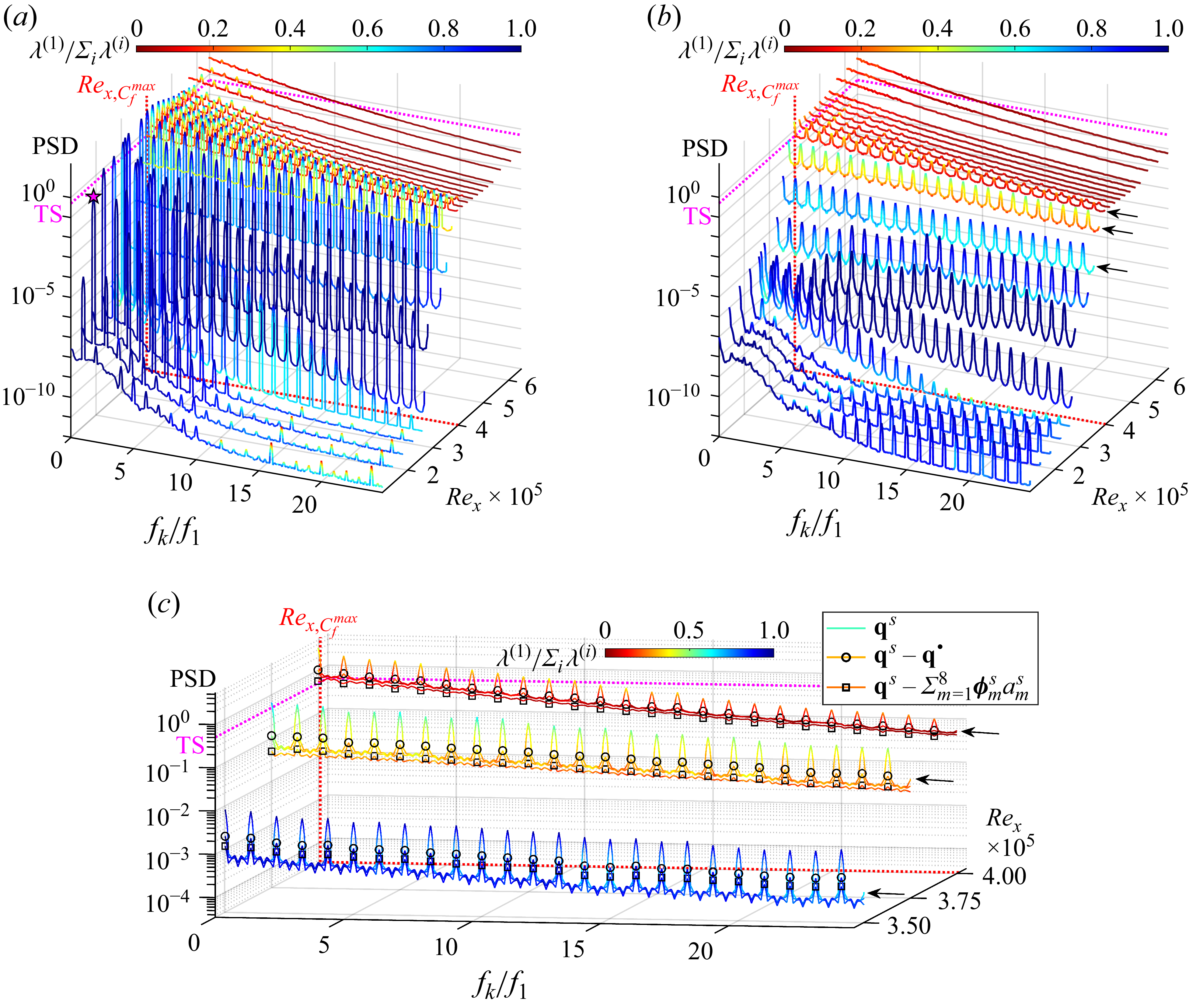
We next adopt a local perspective to gain a better overview of the streamwise evolution of these components. To this end, figure 3 plots local integral- $y^*$
–
$y^*$
– $z^*$
-plane power spectral densities for each streamwise station, coloured by the local SPOD energy ratio
$z^*$
-plane power spectral densities for each streamwise station, coloured by the local SPOD energy ratio $\lambda^{(1)}(x)/\sum _i \lambda^{(i)}(x)$
to quantify the mode dominance. High values (blue) denote energy focused in one leading mode, while low values (red) reflect energy spread across many modes. This spatially resolved analysis reveals the statistics and dynamics that dominate at each location and frequency, guiding a subsequent search for coherent structures. The fundamental spectral evolution starts with the TS wave, marked in figure 3(a), whose energy level we use as reference for other components (above TS, significant; below TS, weak). Its FHR
$\lambda^{(1)}(x)/\sum _i \lambda^{(i)}(x)$
to quantify the mode dominance. High values (blue) denote energy focused in one leading mode, while low values (red) reflect energy spread across many modes. This spatially resolved analysis reveals the statistics and dynamics that dominate at each location and frequency, guiding a subsequent search for coherent structures. The fundamental spectral evolution starts with the TS wave, marked in figure 3(a), whose energy level we use as reference for other components (above TS, significant; below TS, weak). Its FHR $\tilde {\mathbf{q}}$
manifests as dominant peaks that grow with increasing
$\tilde {\mathbf{q}}$
manifests as dominant peaks that grow with increasing ${\textit{Re}}_x$
, while non-harmonic components remain negligible in the weak background spectrum. The initial flow is thus deterministic. As the flow gains energy towards
${\textit{Re}}_x$
, while non-harmonic components remain negligible in the weak background spectrum. The initial flow is thus deterministic. As the flow gains energy towards $C_f^{{\textit{max}}}$
(at
$C_f^{{\textit{max}}}$
(at ${\textit{Re}}_x \approx 4 \times 10^5$
), the non-harmonic spectrum gains amplitude with decreasing mode dominance, indicating increasing stochasticity, while the harmonic peaks lose both amplitude and their initial mode dominance. Since the flow is cyclo-stationary and all its energy is initially confined to
${\textit{Re}}_x \approx 4 \times 10^5$
), the non-harmonic spectrum gains amplitude with decreasing mode dominance, indicating increasing stochasticity, while the harmonic peaks lose both amplitude and their initial mode dominance. Since the flow is cyclo-stationary and all its energy is initially confined to $\tilde {\mathbf{q}}$
(see figure 4
c), the emergence of broadband content reflects energy transfer from the harmonics to
$\tilde {\mathbf{q}}$
(see figure 4
c), the emergence of broadband content reflects energy transfer from the harmonics to ${\mathbf{q}}^s$
, marking the transition from periodic to time-symmetry-broken states. Beyond
${\mathbf{q}}^s$
, marking the transition from periodic to time-symmetry-broken states. Beyond $C_f^{{\textit{max}}}$
, the spectrum converges towards a fully broadband, low modal dominance state, indicating statistical stationarity and turbulence.
$C_f^{{\textit{max}}}$
, the spectrum converges towards a fully broadband, low modal dominance state, indicating statistical stationarity and turbulence.
Remarkably, figure 3(b) shows that even after removing the deterministic FHR $\tilde {\mathbf{q}}$
, the
$\tilde {\mathbf{q}}$
, the ${\mathbf{q}}^s$
fluctuation spectrum still exhibits prominent harmonic peaks with high modal dominance. This crucial finding indicates that fluctuations remain largely phase-locked to the harmonics initially and can also be represented by few dominant modes at these frequencies, thereby motivating a targeted search for coherent structures that dominate symmetry breaking.
${\mathbf{q}}^s$
fluctuation spectrum still exhibits prominent harmonic peaks with high modal dominance. This crucial finding indicates that fluctuations remain largely phase-locked to the harmonics initially and can also be represented by few dominant modes at these frequencies, thereby motivating a targeted search for coherent structures that dominate symmetry breaking.
(a) ${\mathbf{q}}^s$
symmetric and (b)
${\mathbf{q}}^s$
symmetric and (b) ${\mathbf{q}}^a$
anti-symmetric STPOD modal energy spectra; dominant modes with periodic dynamics coloured magenta. (c) Streamwise amplitude development of select STPOD modes
${\mathbf{q}}^a$
anti-symmetric STPOD modal energy spectra; dominant modes with periodic dynamics coloured magenta. (c) Streamwise amplitude development of select STPOD modes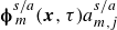 $\boldsymbol{\unicode{x03D5}}^{s/a}_{\,m}({\boldsymbol{x}},\tau ) a^{s/a}_{m,j}$
, enveloped by the total
$\boldsymbol{\unicode{x03D5}}^{s/a}_{\,m}({\boldsymbol{x}},\tau ) a^{s/a}_{m,j}$
, enveloped by the total ${\mathbf{q}}^S$
,
${\mathbf{q}}^S$
, ${\mathbf{q}}^s$
and
${\mathbf{q}}^s$
and ${\mathbf{q}}^{a}$
components. The TS wave input amplitude level serves as significance threshold.
${\mathbf{q}}^{a}$
components. The TS wave input amplitude level serves as significance threshold.

4. Dynamics and statistics of temporal and spatial symmetry breaking
We apply STPOD to the ${\mathbf{q}}^s$
and
${\mathbf{q}}^s$
and ${\mathbf{q}}^a$
fluctuations using the method outlined in § 2.3 to identify dominant symmetry breaking modes with minimal assumptions. As we centre the data around the FHR
${\mathbf{q}}^a$
fluctuations using the method outlined in § 2.3 to identify dominant symmetry breaking modes with minimal assumptions. As we centre the data around the FHR $\tilde {\mathbf{q}}$
(which would otherwise be obtained as the first mode if not subtracted),
$\tilde {\mathbf{q}}$
(which would otherwise be obtained as the first mode if not subtracted), $\tilde {\mathbf{q}}$
can be interpreted as the fundamental space–time mode, leading to the full decomposition
$\tilde {\mathbf{q}}$
can be interpreted as the fundamental space–time mode, leading to the full decomposition
 \begin{equation} {\mathbf{q}}({{\mathbf{x}}},t) = {\mathbf{q}}^s({{\mathbf{x}}},t) + {\mathbf{q}}^a({{\mathbf{x}}},t) + \tilde {\mathbf{q}}({{\mathbf{x}}}, t) = \sum _{m} \left ( \boldsymbol{\unicode{x03D5}}_m^{s}({{\mathbf{x}}},\tau ) a_{m,j}^{s} + \boldsymbol{\unicode{x03D5}}_m^{a}({{\mathbf{x}}},\tau ) a_{m,j}^{a} \right ) + \tilde {\mathbf{q}}({{\mathbf{x}}}, t), \end{equation}
where $a_{m,j}^{s/a}$
with
$a_{m,j}^{s/a}$
with $j\in [1,N_{T_1}]$
are realisation-dependent expansion coefficients describing amplitude modulations of mode
$j\in [1,N_{T_1}]$
are realisation-dependent expansion coefficients describing amplitude modulations of mode $\boldsymbol{\unicode{x03D5}}_m^{s/a}$
across different flow realisations (periods)
$\boldsymbol{\unicode{x03D5}}_m^{s/a}$
across different flow realisations (periods) $j$
. To further resolve the time dynamics of these space–time modes, we propose a modal multi-time scale approach via a nested space-only POD, separating spatial and temporal information:
$j$
. To further resolve the time dynamics of these space–time modes, we propose a modal multi-time scale approach via a nested space-only POD, separating spatial and temporal information:
 \begin{equation} \begin{aligned} \boldsymbol{\unicode{x03D5}}_m({{\mathbf{x}}},\tau) & = {{\mathbf{U}}}_m({\boldsymbol{x}}) {\mathbf{a}}_m^{\mathrm{POD}}(\tau), \\{\mathbf{q}}({{\mathbf{x}}},t) &= \sum _{m} {{\mathbf{U}}}_m({\mathbf{x}}) {\mathbf{a}}_m^{\mathrm{POD}}(\tau) a_{m,j} + {{\mathbf{U}}}_0({{\mathbf{x}}}) {\mathbf{a}}_0^{\mathrm{POD}}(t), \end{aligned} \end{equation}
with space-only POD modes ${\mathbf{U}}_m({\boldsymbol{x}})$
and local POD expansion coefficients
${\mathbf{U}}_m({\boldsymbol{x}})$
and local POD expansion coefficients ${\mathbf{a}}_m^{\mathrm{POD}}(\tau)$
. We choose POD for its
${\mathbf{a}}_m^{\mathrm{POD}}(\tau)$
. We choose POD for its $L_2$
-optimality and objectivity about time dynamics, unlike dynamic mode decomposition or Fourier methods, which assume linear or periodic dynamics. This decomposition now allows for a clear separation of time scales: the fast local dynamics
$L_2$
-optimality and objectivity about time dynamics, unlike dynamic mode decomposition or Fourier methods, which assume linear or periodic dynamics. This decomposition now allows for a clear separation of time scales: the fast local dynamics ${\mathbf{a}}_m^{\mathrm{POD}}(\tau)$
within a realisation (
${\mathbf{a}}_m^{\mathrm{POD}}(\tau)$
within a realisation ( $\tau \in [0,T_1]$
) and slow global modulation
$\tau \in [0,T_1]$
) and slow global modulation $a_{m,j}$
across realisations, where the instantaneous time becomes
$a_{m,j}$
across realisations, where the instantaneous time becomes $t = \tau+(j-1)T_1$
. Furthermore, this enables a dynamical systems analysis by resolving mode trajectory shapes in phase space with
$t = \tau+(j-1)T_1$
. Furthermore, this enables a dynamical systems analysis by resolving mode trajectory shapes in phase space with ${\mathbf{a}}_m^{\mathrm{POD}}(\tau)$
(Cvitanović & Gibson Reference Cvitanović and Gibson2010). For visualisation, plotting the dominant three coefficients of the
${\mathbf{a}}_m^{\mathrm{POD}}(\tau)$
(Cvitanović & Gibson Reference Cvitanović and Gibson2010). For visualisation, plotting the dominant three coefficients of the ${\mathbf{a}}_m^{\mathrm{POD}} (\tau)$
vector typically suffices, as higher coefficients generally remain periodic even when dominant ones are not.
${\mathbf{a}}_m^{\mathrm{POD}} (\tau)$
vector typically suffices, as higher coefficients generally remain periodic even when dominant ones are not.
Symmetry breaking modes from STPOD. Deterministic mode $\tilde {\mathbf{q}}$
(FHR), first three symmetric modes (
$\tilde {\mathbf{q}}$
(FHR), first three symmetric modes ( $\boldsymbol{\unicode{x03D5}}^s_{1-3}$
) and first two anti-symmetric modes (
$\boldsymbol{\unicode{x03D5}}^s_{1-3}$
) and first two anti-symmetric modes ( $\boldsymbol{\unicode{x03D5}}^a_{1-2}$
). (a)
$\boldsymbol{\unicode{x03D5}}^a_{1-2}$
). (a) ${\mathbf{a}}_m^{\mathrm{POD}}(\tau)$
trajectory phase-spaces and (b) instantaneous isosurfaces at same phase. Symmetric modes shown by
${\mathbf{a}}_m^{\mathrm{POD}}(\tau)$
trajectory phase-spaces and (b) instantaneous isosurfaces at same phase. Symmetric modes shown by $Q$
-criterion (
$Q$
-criterion ( $Q=10^3$
) coloured by
$Q=10^3$
) coloured by $u$
-velocity; anti-symmetric modes shown by
$u$
-velocity; anti-symmetric modes shown by $w$
-velocity (
$w$
-velocity ( $w=\pm 0.002$
). (c) Symmetric and (d) anti-symmetric mode relative
$w=\pm 0.002$
). (c) Symmetric and (d) anti-symmetric mode relative $\text{L}_2$
-norm distances between consecutive phases. Red markers denote distance from last to first phase (periodicity mismatch), error bars show the existing min
$\text{L}_2$
-norm distances between consecutive phases. Red markers denote distance from last to first phase (periodicity mismatch), error bars show the existing min $/$
max consecutive phase distances within the period, normalised by the average phase distance in a given mode. See supplementary movie 2.
$/$
max consecutive phase distances within the period, normalised by the average phase distance in a given mode. See supplementary movie 2.

4.1. Onset of quasi-periodicity and aperiodicity
Figure 4 plots the energy spectra and streamwise amplitude development of the STPOD modes. Up to ${\textit{Re}}_x \lesssim 3.5\times 10^5$
, the flow is governed entirely by the deterministic, spatially compact mode (FHR) of the early transition. Figure 4(c) shows that, as
${\textit{Re}}_x \lesssim 3.5\times 10^5$
, the flow is governed entirely by the deterministic, spatially compact mode (FHR) of the early transition. Figure 4(c) shows that, as $\tilde {\mathbf{q}}$
falls below the total amplitude, new dominant symmetric STPOD modes
$\tilde {\mathbf{q}}$
falls below the total amplitude, new dominant symmetric STPOD modes $\boldsymbol{\unicode{x03D5}}_1^s$
and
$\boldsymbol{\unicode{x03D5}}_1^s$
and $\boldsymbol{\unicode{x03D5}}_2^s$
surge above the TS wave level at
$\boldsymbol{\unicode{x03D5}}_2^s$
surge above the TS wave level at ${\textit{Re}}_x \approx 3.5\times 10^5$
. They too are vortical and compact, seen in figure 5(b), and mark the onset of variance from the purely periodic
${\textit{Re}}_x \approx 3.5\times 10^5$
. They too are vortical and compact, seen in figure 5(b), and mark the onset of variance from the purely periodic $\tilde {\mathbf{q}}$
. The phase space analysis in figure 5(a,c) reveals that these modes, remarkably, also exhibit
$\tilde {\mathbf{q}}$
. The phase space analysis in figure 5(a,c) reveals that these modes, remarkably, also exhibit $T_1$
-periodic dynamics:
$T_1$
-periodic dynamics:
 \begin{equation} \boldsymbol{\unicode{x03D5}}_m^s \left ( \boldsymbol{x}, \tau \rightarrow T_1 \right ) \begin{cases} = \boldsymbol{\unicode{x03D5}}_m^s \left ( {\mathbf{x}}, \tau \rightarrow 0 \right ), & m=\{1,2\}, \\ \neq \boldsymbol{\unicode{x03D5}}_m^s \left ( {\mathbf{x}}, \tau \rightarrow 0 \right ), & m \geqslant 3. \end{cases} \end{equation}
The critical distinction lies in their non-constant expansion coefficients $a_{1,j}^s$
and
$a_{1,j}^s$
and $a_{2,j}^s$
that vary over long time scales. This creates a region of geometrically quasi-periodic dynamics where the state is modulated by different periodic trajectories, i.e. for
$a_{2,j}^s$
that vary over long time scales. This creates a region of geometrically quasi-periodic dynamics where the state is modulated by different periodic trajectories, i.e. for $3.4\times 10^5 \lesssim Re_x \lesssim 3.7\times 10^5$
,
$3.4\times 10^5 \lesssim Re_x \lesssim 3.7\times 10^5$
,
 \begin{equation} {\mathbf{q}}({{\mathbf{x}}},t) \approx \tilde {\mathbf{q}}({{\mathbf{x}}},t) + {\mathbf{q}}^{\bullet }({{\mathbf{x}}},t) = \tilde {\mathbf{q}}({{\mathbf{x}}}, t) + a_{1,j}^s\boldsymbol{\unicode{x03D5}}_1^s({{\mathbf{x}}},\tau) + a_{2,j}^s \boldsymbol{\unicode{x03D5}}_2^s({{\mathbf{x}}},\tau). \end{equation}
These trajectories are statistically periodic, but instantaneously depart from the deterministic state $\tilde {\mathbf{q}}$
in shapes and directions given by
$\tilde {\mathbf{q}}$
in shapes and directions given by $\boldsymbol{\unicode{x03D5}}_1^s$
and
$\boldsymbol{\unicode{x03D5}}_1^s$
and $\boldsymbol{\unicode{x03D5}}_2^s$
, with amplitudes and timings governed explicitly by expansion coefficients
$\boldsymbol{\unicode{x03D5}}_2^s$
, with amplitudes and timings governed explicitly by expansion coefficients $a_{1,j}^s$
and
$a_{1,j}^s$
and $a_{2,j}^s$
that vary slowly over the periods
$a_{2,j}^s$
that vary slowly over the periods $j$
. This quasi-periodic dynamic is a categorical departure from the previous deterministic behaviour, as the system now explores multiple periodic trajectories in a structured manner.
$j$
. This quasi-periodic dynamic is a categorical departure from the previous deterministic behaviour, as the system now explores multiple periodic trajectories in a structured manner.
The onset of chaos begins with the emergence of $\boldsymbol{\unicode{x03D5}}_3^s$
around
$\boldsymbol{\unicode{x03D5}}_3^s$
around ${\textit{Re}}_x \gtrsim 3.7\times 10^5$
. This mode breaks the pattern of local periodicity, exhibiting a clear jump between its first and last phase (figure 5
a,c). All higher modes (
${\textit{Re}}_x \gtrsim 3.7\times 10^5$
. This mode breaks the pattern of local periodicity, exhibiting a clear jump between its first and last phase (figure 5
a,c). All higher modes ( $m \geqslant 3$
) are also aperiodic and located increasingly further downstream. This creates the spectral redistribution from harmonic to broadband frequencies, shown in figure 3(c). A zoom into the region of critical fluctuation growth reveals the spectral contents of the modes. Removing the periodic modes
$m \geqslant 3$
) are also aperiodic and located increasingly further downstream. This creates the spectral redistribution from harmonic to broadband frequencies, shown in figure 3(c). A zoom into the region of critical fluctuation growth reveals the spectral contents of the modes. Removing the periodic modes $\boldsymbol{\unicode{x03D5}}_1^s$
and
$\boldsymbol{\unicode{x03D5}}_1^s$
and $\boldsymbol{\unicode{x03D5}}_2^s$
eliminates precisely the mode-dominant harmonic peaks, while removing higher modes flattens the spectrum across all frequencies towards fully broadband characteristics. Since modes that are not
$\boldsymbol{\unicode{x03D5}}_2^s$
eliminates precisely the mode-dominant harmonic peaks, while removing higher modes flattens the spectrum across all frequencies towards fully broadband characteristics. Since modes that are not $T_1$
-periodic can, by definition, not be captured solely within the harmonic frequencies, they must fill the broadband spectrum between peaks, and are thus indicative of chaos and turbulence.
$T_1$
-periodic can, by definition, not be captured solely within the harmonic frequencies, they must fill the broadband spectrum between peaks, and are thus indicative of chaos and turbulence.
The progression from periodic to chaotic dynamics seen here echoes the dynamical systems view of wall turbulence (Cvitanović & Gibson Reference Cvitanović and Gibson2010; Kawahara & Kida Reference Kawahara and Kida2001; Viswanath Reference Viswanath2007), where trajectories recurrently visit the available unstable periodic orbits that ‘scaffold’ the state space. Our hierarchical breakdown – from a single periodic base state ( $\tilde {\mathbf{q}}$
), through quasi-periodic modulations (
$\tilde {\mathbf{q}}$
), through quasi-periodic modulations ( $\boldsymbol{\unicode{x03D5}}_1^s$
,
$\boldsymbol{\unicode{x03D5}}_1^s$
, $\boldsymbol{\unicode{x03D5}}_2^s$
), to chaotic excursions via non-periodic modes (
$\boldsymbol{\unicode{x03D5}}_2^s$
), to chaotic excursions via non-periodic modes ( $\boldsymbol{\unicode{x03D5}}_3^s$
and higher) – offers a data-driven perspective on this mechanism.
$\boldsymbol{\unicode{x03D5}}_3^s$
and higher) – offers a data-driven perspective on this mechanism.
4.2. Onset of spanwise asymmetry
Spatial symmetry breaking follows a remarkably similar route. The anti-symmetric component ${\mathbf{q}}^A = {\mathbf{q}}^a$
remains energetically negligible until
${\mathbf{q}}^A = {\mathbf{q}}^a$
remains energetically negligible until ${\textit{Re}}_x\lesssim 3.8\times 10^5$
(figure 4
c), from where it rapidly amplifies towards the amplitude of
${\textit{Re}}_x\lesssim 3.8\times 10^5$
(figure 4
c), from where it rapidly amplifies towards the amplitude of ${\mathbf{q}}^S$
. To isolate the modes that initiate asymmetry onset, we compute the STPOD for
${\mathbf{q}}^S$
. To isolate the modes that initiate asymmetry onset, we compute the STPOD for ${\mathbf{q}}^a$
with a spatial weight focused on the amplified region of interest (
${\mathbf{q}}^a$
with a spatial weight focused on the amplified region of interest ( ${\textit{Re}}_x \leqslant 4.0\times 10^5$
) prior to the onset of saturated downstream turbulence. Most notably, the first anti-symmetric mode
${\textit{Re}}_x \leqslant 4.0\times 10^5$
) prior to the onset of saturated downstream turbulence. Most notably, the first anti-symmetric mode $\boldsymbol{\unicode{x03D5}}_1^a$
also exhibits local periodicity (figure 5
a,d)
$\boldsymbol{\unicode{x03D5}}_1^a$
also exhibits local periodicity (figure 5
a,d)
 \begin{equation} \boldsymbol{\unicode{x03D5}}_m^a \left ( {\mathbf{x}}, \tau \rightarrow T_1 \right ) \begin{cases} = \boldsymbol{\unicode{x03D5}}_m^a \left ( {\mathbf{x}}, \tau \rightarrow 0 \right ), & m = 1, \\ \neq \boldsymbol{\unicode{x03D5}}_m^a \left ( {\mathbf{x}}, \tau \rightarrow 0 \right ), & m \geqslant 2, \end{cases} \end{equation}
despite a total absence of anti-symmetric forcing or mean flow. Similar to (4.4), $\boldsymbol{\unicode{x03D5}}_1^a$
forms quasi-periodic asymmetric variations with
$\boldsymbol{\unicode{x03D5}}_1^a$
forms quasi-periodic asymmetric variations with $\tilde {\mathbf{q}}$
, while spectral analysis analogous to figure 3(b,c) (omitted for brevity) confirms that higher modes again become broadband. Thus, a central finding here is that both spatial and temporal symmetry breaking emerge through coherent space–time structures in distinct dynamical hierarchies, not as random fluctuations.
$\tilde {\mathbf{q}}$
, while spectral analysis analogous to figure 3(b,c) (omitted for brevity) confirms that higher modes again become broadband. Thus, a central finding here is that both spatial and temporal symmetry breaking emerge through coherent space–time structures in distinct dynamical hierarchies, not as random fluctuations.
5. Inter-modal $/$
inter-symmetry energy transfer
$/$
inter-symmetry energy transfer

We introduce the symmetry-decomposed Navier–Stokes equations (NSE). By inserting the decomposition (2.2) into the incompressible NSE, followed by reflection about the symmetry plane and subsequent addition or subtraction of the reflection, we obtain respectively
 \begin{align} \hspace {-14pt}\text{(Symmetric NSE)}\;\;\hspace {5pt} \partial _t u_i^{S} {\kern-1pt} +{\kern-.5pt} u_j^S\,\partial _{x\!_j} u_i^{S}{\kern-1pt} +{\kern-.5pt} u_j^{A}\,\partial _{x\!_j} u_i^{A} &= -\partial \!_{x_i} p^{S} {\kern-1pt} +{\kern-.5pt} \nu \,\partial _{{x\!_j}{x\!_j}} u_i^{S}, \hspace {8pt} \partial \!_{x_i} u_i^{S}=0, \end{align}
 \begin{align} \hspace {-5pt}\text{(Anti-sym. NSE)}\;\;\hspace {5pt} \partial _t u_i^{A} {\kern-1pt} +{\kern-.5pt} u_j^{S}\,\partial _{x\!_j} u_i^{A} {\kern-1pt} +{\kern-.5pt} u_j^{A}\,\partial _{x\!_j} u_i^{S} &= -\partial \!_{x_i} p^{A} {\kern-1pt} +{\kern-.5pt} \nu \,\partial _{x\!_j x\!_j} u_i^{A}, \hspace {6pt} \partial \!_{x_i} u_i^{A}=0. \end{align}
As the cyclo-stationary anti-symmetric component is purely fluctuating ( $u_i^{A}=u_i^{a}$
), its energy budget follows from dotting (5.2) with
$u_i^{A}=u_i^{a}$
), its energy budget follows from dotting (5.2) with $u_i^{a}$
and phase-averaging
$u_i^{a}$
and phase-averaging $\widetilde {(\boldsymbol{\cdot })}$
, yielding the equation
$\widetilde {(\boldsymbol{\cdot })}$
, yielding the equation

in which the production pathway is shear extraction from the symmetric field consisting of FHR ( $\mathcal{P}^{\star \to a}$
) and turbulent (
$\mathcal{P}^{\star \to a}$
) and turbulent ( $\mathcal{P}^{s\to a}$
) production for a phase-averaged TKE
$\mathcal{P}^{s\to a}$
) production for a phase-averaged TKE  . For the symmetric NSE, we insert the cyclo-stationary decomposition $u_i^{S} = \widetilde {u}_i + u_i^{s}$
, and take dot products with
$u_i^{S} = \widetilde {u}_i + u_i^{s}$
, and take dot products with $\widetilde {u}_i$
and
$\widetilde {u}_i$
and $u_i^{s}$
each, followed by phase-averaging, to derive TKE budgets
$u_i^{s}$
each, followed by phase-averaging, to derive TKE budgets $k^{\star }\equiv \widetilde {u}_i \widetilde {u}_i/2$
and
$k^{\star }\equiv \widetilde {u}_i \widetilde {u}_i/2$
and  for the FHR and the symmetric fluctuations, respectively,


The three budgets are linked by pairs of equal-and-opposite production terms, which create directed energy transfers via harmonic ( $\mathcal{P}^{\star \to s}$
,
$\mathcal{P}^{\star \to s}$
, $\mathcal{P}^{\star \to a}$
) or inter-symmetry (
$\mathcal{P}^{\star \to a}$
) or inter-symmetry ( $\mathcal{P}^{s\to a}$
) pathways. Similarly, we derive an inter-modal energy transfer between the leading modes of each symmetry class and their residual turbulent fluctuations. The symmetric fluctuation is split into
$\mathcal{P}^{s\to a}$
) pathways. Similarly, we derive an inter-modal energy transfer between the leading modes of each symmetry class and their residual turbulent fluctuations. The symmetric fluctuation is split into $u_i^{s}=u_i^{\bullet }+u_i^{\circ }$
. With the respective dot products and phase-averaging, the TKE budget of the leading quasi-periodic symmetric modes (i.e.
$u_i^{s}=u_i^{\bullet }+u_i^{\circ }$
. With the respective dot products and phase-averaging, the TKE budget of the leading quasi-periodic symmetric modes (i.e. ${\mathbf{q}}^{\bullet } \!=\! a_{1}^s\boldsymbol{\unicode{x03D5}}_{1}^s \!+ \! a_{2}^s\boldsymbol{\unicode{x03D5}}_{2}^s$
) is derived as
${\mathbf{q}}^{\bullet } \!=\! a_{1}^s\boldsymbol{\unicode{x03D5}}_{1}^s \!+ \! a_{2}^s\boldsymbol{\unicode{x03D5}}_{2}^s$
) is derived as

and the TKE budget for the symmetric residual fluctuation is given by a conjugate equation

We note that the sum of (5.6) and (5.7) exactly recovers the total symmetric TKE budget (5.5). Both feature conjugate source terms, $\mathcal{S}^{\circ \to \bullet }$
and
$\mathcal{S}^{\circ \to \bullet }$
and $\mathcal{S}^{\bullet \to \circ }$
, that couple the energy flow between the leading modes and residual fluctuations, as well as standard production terms by the FHR (
$\mathcal{S}^{\bullet \to \circ }$
, that couple the energy flow between the leading modes and residual fluctuations, as well as standard production terms by the FHR ( $\mathcal{P}^{\star \to \bullet /\circ }$
) and, notably, interaction terms with the anti-symmetric fluctuation
$\mathcal{P}^{\star \to \bullet /\circ }$
) and, notably, interaction terms with the anti-symmetric fluctuation $(\mathcal{T}^{\bullet /\circ \leftarrow a}\!-\mathcal{P}^{\bullet /\circ \rightarrow a})$
. Thus, we apply the split
$(\mathcal{T}^{\bullet /\circ \leftarrow a}\!-\mathcal{P}^{\bullet /\circ \rightarrow a})$
. Thus, we apply the split $u_i^{a}=u_i^{{\blacktriangle }}+u_i^{{\vartriangle }}$
to likewise derive the TKE budget of the leading quasi-periodic anti-symmetric mode
$u_i^{a}=u_i^{{\blacktriangle }}+u_i^{{\vartriangle }}$
to likewise derive the TKE budget of the leading quasi-periodic anti-symmetric mode $m=1$
(i.e.
$m=1$
(i.e. ${\mathbf{q}}^{{\blacktriangle }}\!=a_{1}^a\boldsymbol{\unicode{x03D5}}_{1}^a$
) as
${\mathbf{q}}^{{\blacktriangle }}\!=a_{1}^a\boldsymbol{\unicode{x03D5}}_{1}^a$
) as

and the respective conjugate TKE budget for the anti-symmetric residual fluctuation as

Again, both (5.8) and (5.9) feature conjugate source terms ( $\mathcal{S}^{{\vartriangle }\to {\blacktriangle }}$
,
$\mathcal{S}^{{\vartriangle }\to {\blacktriangle }}$
, $\mathcal{S}^{{\blacktriangle }\to {\vartriangle }}$
), production terms with FHR and symmetric fluctuations, and recombine to form the total budget (5.3).
$\mathcal{S}^{{\blacktriangle }\to {\vartriangle }}$
), production terms with FHR and symmetric fluctuations, and recombine to form the total budget (5.3).
Inter-modal/inter-symmetry energy transfer and production terms. (a) Symmetric and (b) anti-symmetric terms in integral- $y^*$
, time-averaged view. (c,d) Integral-
$y^*$
, time-averaged view. (c,d) Integral- $y^*$
–
$y^*$
– $z^*$
, time-averaged view, normalised by their total TKE (and small
$z^*$
, time-averaged view, normalised by their total TKE (and small $\epsilon$
to avoid division by 0), yielding a TKE-specific efficacy of each pathway relative to the local energy. See supplementary movie 3. Legend: (
$\epsilon$
to avoid division by 0), yielding a TKE-specific efficacy of each pathway relative to the local energy. See supplementary movie 3. Legend: ( $\bullet /\circ$
) quasi-periodic
$\bullet /\circ$
) quasi-periodic $/$
residual symmetric; (
$/$
residual symmetric; ( $\blacktriangle /\triangle$
) quasi-periodic
$\blacktriangle /\triangle$
) quasi-periodic $/$
residual anti-symmetric; (
$/$
residual anti-symmetric; ( $\star$
) FHR.
$\star$
) FHR.

Figure 6 reveals that in both symmetry classes, the production from the FHR to the leading modes ( $\mathcal{P}^{\star \rightarrow \bullet /{\blacktriangle }}$
) arises and peaks upstream of their residual production (
$\mathcal{P}^{\star \rightarrow \bullet /{\blacktriangle }}$
) arises and peaks upstream of their residual production ( $\mathcal{P}^{\star \rightarrow \circ /{\vartriangle }}$
). This establishes a distinct streamwise succession: dominant modes are energised first by the FHR, serving as precursor for the subsequent growth of residual fluctuations. The mechanism underlying this transition is the inter-modal transfer, which exhibits an equal-and-opposite source-sink structure, i.e.
$\mathcal{P}^{\star \rightarrow \circ /{\vartriangle }}$
). This establishes a distinct streamwise succession: dominant modes are energised first by the FHR, serving as precursor for the subsequent growth of residual fluctuations. The mechanism underlying this transition is the inter-modal transfer, which exhibits an equal-and-opposite source-sink structure, i.e. $\mathcal{S}^{\bullet \rightarrow \circ }\!\approx \! -\mathcal{S}^{\circ \rightarrow \bullet }$
and
$\mathcal{S}^{\bullet \rightarrow \circ }\!\approx \! -\mathcal{S}^{\circ \rightarrow \bullet }$
and $\mathcal{S}^{{\blacktriangle }\rightarrow {\vartriangle }}\!\approx \! -\mathcal{S}^{{\vartriangle }\rightarrow {\blacktriangle }}$
, visible in both their
$\mathcal{S}^{{\blacktriangle }\rightarrow {\vartriangle }}\!\approx \! -\mathcal{S}^{{\vartriangle }\rightarrow {\blacktriangle }}$
, visible in both their ${\textit{Re}}_x$
–
${\textit{Re}}_x$
– $z^*$
footprints and line plots. Accordingly, we report only the transfer
$z^*$
footprints and line plots. Accordingly, we report only the transfer $/$
production terms essential for energetic coupling of the TKE budgets (transport terms
$/$
production terms essential for energetic coupling of the TKE budgets (transport terms $\mathcal{T}$
are numerically negligible). Most notably, the residual production arises only in lockstep with the inter-modal transfer, and not before or independently, implying a handoff mechanism wherein the residual field does not grow until energised by the transfer from the leading modes. This sequenced, directed energy transfer suggests that the leading modes act as energetic gateway, enabling the flow of energy from the deterministic FHR to the broadband turbulent residuals.
$\mathcal{T}$
are numerically negligible). Most notably, the residual production arises only in lockstep with the inter-modal transfer, and not before or independently, implying a handoff mechanism wherein the residual field does not grow until energised by the transfer from the leading modes. This sequenced, directed energy transfer suggests that the leading modes act as energetic gateway, enabling the flow of energy from the deterministic FHR to the broadband turbulent residuals.
In the anti-symmetric case, the residual production $\mathcal{P}^{\star \rightarrow {\vartriangle }}$
, once energised via
$\mathcal{P}^{\star \rightarrow {\vartriangle }}$
, once energised via $\mathcal{S}^{{\blacktriangle }\rightarrow {\vartriangle }}$
, rapidly exceeds the efficacy of the mode production as it peaks in tandem with the nonlinear inter-symmetry production
$\mathcal{S}^{{\blacktriangle }\rightarrow {\vartriangle }}$
, rapidly exceeds the efficacy of the mode production as it peaks in tandem with the nonlinear inter-symmetry production $\mathcal{P}^{s\rightarrow {\vartriangle }}$
. This term acts as a potent source for the anti-symmetric residual and as sink for the symmetric budget (green dashed lines in figure 6
c,d), confirming negligible back-coupling (i.e.
$\mathcal{P}^{s\rightarrow {\vartriangle }}$
. This term acts as a potent source for the anti-symmetric residual and as sink for the symmetric budget (green dashed lines in figure 6
c,d), confirming negligible back-coupling (i.e. $(\mathcal{T}^{s\leftarrow {\vartriangle }}\!\!-\!\mathcal{P}^{s\rightarrow {\vartriangle }}) \!\approx \! -\mathcal{P}^{s\rightarrow {\vartriangle }}$
). Its rise occurs downstream of the initial mode production
$(\mathcal{T}^{s\leftarrow {\vartriangle }}\!\!-\!\mathcal{P}^{s\rightarrow {\vartriangle }}) \!\approx \! -\mathcal{P}^{s\rightarrow {\vartriangle }}$
). Its rise occurs downstream of the initial mode production $\mathcal{P}^{\star \rightarrow {\blacktriangle }}$
and in tandem with the surging residual production, suggesting a sequenced breakdown: anti-symmetry initially arises via the dominant mode, but is subsequently amplified by nonlinear inter-symmetry transfer to produce the anti-symmetric broadband residual. Across all energy pathways, the quantities are spatially coherent in the
$\mathcal{P}^{\star \rightarrow {\blacktriangle }}$
and in tandem with the surging residual production, suggesting a sequenced breakdown: anti-symmetry initially arises via the dominant mode, but is subsequently amplified by nonlinear inter-symmetry transfer to produce the anti-symmetric broadband residual. Across all energy pathways, the quantities are spatially coherent in the ${\textit{Re}}_x$
–
${\textit{Re}}_x$
– $z^*$
plane (figure 6
a,b), demonstrating that symmetry-broken turbulence is energetically driven by space–time coherent modes rather than random noise.
$z^*$
plane (figure 6
a,b), demonstrating that symmetry-broken turbulence is energetically driven by space–time coherent modes rather than random noise.
6. Concluding remarks
This work reveals the temporal and spatial symmetry breaking mechanisms in canonical K-type boundary layer transition. Deterministic transition begins with eigen-modal dynamics at a single frequency (TS wave) that evolve into harmonics through quadratic nonlinear interactions. This fundamental harmonic response (FHR) $\tilde {\mathbf{q}}$
is composed entirely of symmetric and periodic coherent structures, is spatially compact and persists far downstream. While
$\tilde {\mathbf{q}}$
is composed entirely of symmetric and periodic coherent structures, is spatially compact and persists far downstream. While $\tilde {\mathbf{q}}$
may resemble turbulence, it remains fully harmonic, clearly defining the extent of the deterministic regime. The ability to pinpoint where deterministic dynamics transition to symmetry breaking provides new clarity in distinguishing organised transition from turbulence onset.
$\tilde {\mathbf{q}}$
may resemble turbulence, it remains fully harmonic, clearly defining the extent of the deterministic regime. The ability to pinpoint where deterministic dynamics transition to symmetry breaking provides new clarity in distinguishing organised transition from turbulence onset.
We identify the specific space–time structures that drive this transition. The FHR $\tilde {\mathbf{q}}$
dominates until
$\tilde {\mathbf{q}}$
dominates until ${\textit{Re}}_x \!\approx \! 3.5\times 10^5$
, after which organised symmetry-breaking structures emerge. The dominant two symmetric modes (
${\textit{Re}}_x \!\approx \! 3.5\times 10^5$
, after which organised symmetry-breaking structures emerge. The dominant two symmetric modes ( $\boldsymbol{\unicode{x03D5}}_1^s$
,
$\boldsymbol{\unicode{x03D5}}_1^s$
, $\boldsymbol{\unicode{x03D5}}_2^s$
) exhibit periodic dynamics with slow amplitude modulation, thereby deviating from the periodic base state in the form of quasi-periodic trajectories and creating variance around the harmonic peaks. With increasing
$\boldsymbol{\unicode{x03D5}}_2^s$
) exhibit periodic dynamics with slow amplitude modulation, thereby deviating from the periodic base state in the form of quasi-periodic trajectories and creating variance around the harmonic peaks. With increasing ${\textit{Re}}_x$
, higher modes (
${\textit{Re}}_x$
, higher modes ( $\boldsymbol{\unicode{x03D5}}_3^s$
and beyond) break periodicity and fill the broadband spectrum, delineating the transition to chaos and turbulence. Notably, spatial symmetry breaking follows a similar organised pattern: despite no anti-symmetric forcings, the first anti-symmetric mode (
$\boldsymbol{\unicode{x03D5}}_3^s$
and beyond) break periodicity and fill the broadband spectrum, delineating the transition to chaos and turbulence. Notably, spatial symmetry breaking follows a similar organised pattern: despite no anti-symmetric forcings, the first anti-symmetric mode ( $\boldsymbol{\unicode{x03D5}}_1^a$
) exhibits periodic dynamics, while higher modes are aperiodic and broadband. This shows that both types of symmetry breaking unfold not as random unstructured fluctuations, but through a hierarchy of emergent, energetically dominant space–time structures, challenging traditional views of symmetry breaking being a purely random process.
$\boldsymbol{\unicode{x03D5}}_1^a$
) exhibits periodic dynamics, while higher modes are aperiodic and broadband. This shows that both types of symmetry breaking unfold not as random unstructured fluctuations, but through a hierarchy of emergent, energetically dominant space–time structures, challenging traditional views of symmetry breaking being a purely random process.
We derive inter-modal and inter-symmetry energy budgets by decomposing the Navier–Stokes equations into symmetric and anti-symmetric governing equations. These budgets reveal conjugate inter-modal source terms that exhibit a numerically confirmed equal-and-opposite conservation, thereby coupling the quasi-periodic modes and the broadband residual fluctuations with a directed energy transfer from the former to the latter. In both symmetry classes, the leading modes are energised first by the FHR, while the residual production arises only as the inter-modal transfer becomes active, and not independently, indicating that the leading modes provide the energetic conduit for broadband residual growth. The anti-symmetric residual surge is dominated by a near-one-way inter-symmetry transfer from the symmetric fluctuations, suggesting that once asymmetry is even weakly present, the inevitable non-periodicity becomes a robust route for rapid amplification of broadband asymmetry.
Crucially, these findings allow us to define both the onset and spatial reach of new regimes, offering new criteria for quantifying, predicting and potentially controlling transition. The resulting hierarchy, from a deterministic periodic state through quasi-periodic modulation to aperiodic broadband dynamics, provides new insight into the structure and dynamics governing the canonical laminar–turbulent transition. While the exact onset location, extent or amplitude of the symmetry-breaking components can vary with configuration or disturbance level, the presented methods provide a broadly applicable framework that isolates symmetry components, identifies dominant structures, and quantifies both the location and the energetic mechanism by which deterministic states evolve to broadband turbulence.
Supplementary movies
Supplementary movies are available at https://doi.org/10.1017/jfm.2026.11423.
Funding
We gratefully acknowledge the NSF for funding this research under grant CBET 2046311.
Declaration of interests
The authors report no conflict of interest.




 Open access

