





1. Introduction
Regional climate models (RCMs) are indispensable for studying the Antarctic Ice Sheet (AIS) and other remote glacierized regions, as they simulate numerous climate variables, including melt and accumulation, where in-situ data are scarce (e.g. van Wessem and others, Reference van Wessem2018; Agosta and others, Reference Agosta2019; Bozkurt and others, Reference Bozkurt, Bromwich, Carrasco and Roberto2021; Mottram and others, Reference Mottram2021), and remote sensing techniques face limitations due to cloud cover, temporal resolution, and limited capacity to quantify melt volumes directly (Trusel and others, Reference Trusel, Frey, Das, Kuipers Munneke and van den Broeke2013; Husman and others, Reference de Roda Husman, Hu, Wouters, Kuipers Munneke, Veldhuijsen and Lhermitte2023). To increase the reliability of future projections, RCMs must be rigorously evaluated against observational data. This study addresses this need by introducing a two-step evaluation framework for RCM validation, designed to ensure that these models provide credible results when applied to future climate scenarios.
The two-step evaluation procedure begins with assessing the RCM’s ability to simulate contemporary surface mass balance (SMB) components when forced with state-of-the-art reanalysis data (step 1). This first step is necessary to assess the ability of RCMs to reproduce the contemporary climate, as well as specific, historical events, and may therefore be regarded as the classical model evaluation. If the agreement between the reanalysis-forced model run and the observations is satisfactory, the model is further tested by comparing the reanalysis forced run with a historical run forced by free-running Earth System Model (ESM), which is also to be used for the future forcing (step 2). This second step is necessary to ensure that the RCM performance is retained for a different forcing, even though the ESM forcing will not reproduce the specific timing of meteorological events. The two-step approach allows for a systematic assessment of the RCM’s robustness under different forcing conditions, building confidence that the model can accurately simulate future changes. We illustrate this process using the RCM RACMO2.3p2 over the Antarctic ice sheet, forced with ERA5 reanalysis and the Earth System Model CESM2, focusing on melt and accumulation rates as representative components of the AIS climate and surface mass balance.
As a demonstration of this two-step process, it is first evaluated whether RACMO2.3p2 can replicate a known historical melt event over the Ross Ice Shelf, comparing simulated melt and temperature with passive microwave satellite observations and automatic weather station (AWS) data. This specific melt event was chosen since continent-wide and multi-annual melt in RACMO2.3p2 has already been extensively evaluated using historical observations (van Wessem and others, Reference van Wessem2018, Reference van Wessem, van den Broeke, Wouters and Lhermitte2023; Jakobs and others, Reference Jakobs, Reijmer, Smeets, Trusel, van de Berg, van den Broeke and van Wessem2020). The January 2016 melt event over the Ross Ice Shelf is well-documented yet poorly reproduced by current RCMs (Nicolas and others, Reference Nicolas2017; Hansen and others, Reference Hansen2024). Then, in step 2 RACMO2.3p2 forced by Earth System Model CESM2 (Danabasoglu and others, Reference Danabasoglu2020) is compared to RACMO2.3p2 forced by ERA5 reanalysis data (Hersbach and others, Reference Hersbach2020) for the same period (1979–2014), based on annual mean, variability, and linear trends, providing a measure of consistency across different forcing datasets.
As an example application we focus on the melt-over-accumulation (MoA) ratio, a key metric for future atmospheric impacts on AIS stability, specifically for its ice shelves. These ice shelves act as buttresses, stabilizing the flow of ice from the continent’s interior (Bennett and Glasser, Reference Bennett and Glasser2009). Aside from ocean-driven processes, the future viability of Antarctic ice shelves is highly dependent on the balance between surface melt and accumulation, as their ratio determines the likelihood of melt ponding and subsequent ice-shelf disintegration through hydrofracture (Kuipers Munneke and others, Reference Kuipers Munneke, Ligtenberg, Van Den Broeke and Vaughan2014; van Wessem and others, Reference van Wessem, van den Broeke, Wouters and Lhermitte2023). Disintegration events, such as those of Larsen A and B in the Antarctic Peninsula, have been linked to prolonged melt ponding on the ice-shelf surface (Doake and others, Reference Doake, Corr, Rott, Skvarca and Young1998; McGrath and others, Reference McGrath, Steffen, Rajaram, Scambos, Abdalati and Rignot2012; Banwell and others, Reference Banwell, MacAyeal and Sergienko2013), making the Antarctic-wide MoA ratio one of the variables relevant for quantifying future ice-shelf stability. By ensuring that RACMO2.3p2 can reliably simulate contemporary MoA under both reanalysis and historical CESM2 forcing, confidence in its MoA projections for future scenarios is enhanced. Based on the outcomes, MoA ratios will be analysed under three climate trajectories (SSP1-2.6, SSP2-4.5, and SSP5-8.5), providing insights into how Antarctic ice shelves and the broader ice sheet may respond to different emission scenarios.
2. Methodology
2.1. Regional atmospheric climate model
Gridded climate data from the Regional Atmospheric Climate Model RACMO2.3p2 with a horizontal resolution of 27 km is utilized. RACMO2.3p2 is a limited area model, which is used to simulate Antarctic climate and surface mass balance (van Wessem and others, Reference van Wessem2018). The model is forced at the lateral and ocean boundaries by either observation-based ECMWF Re-Analysis data (ERA5, 1979-2022) (Hersbach and others, Reference Hersbach2020) or by the free-running (not observationally constrained) Community Earth System Model (CESM2). CESM2 couples the ocean, atmosphere and land systems (Danabasoglu and others, Reference Danabasoglu2020). The climate data provided by RACMO2.3p2 is analysed using Python version 3.12. Throughout this study, data with various temporal resolution is utilized, namely, 3-hourly-averaged, daily-averaged, and monthly-summed. Variations in precipitation, near-surface temperature, sublimation and surface snowmelt across the AIS are deduced from the RACMO2.3p2 output data. For the evaluation of future MoA values three SSP projection scenarios (O’Neill and others, Reference O’Neill2017) are used, namely SSP1-2.6, SSP2-4.5 and SSP5-8.5, representing scenarios with low, middle and high emission of greenhouse gases.
2.2. Two-step evaluation
Step 1 of the model evaluation constitutes the ability of ERA5-forced RACMO2.3p2 to simulate contemporary climate. When found satisfactory, step 2 constitutes the ability of CESM2-forced RACMO2.3p2 to reproduce this climate for the overlapping historical period.
To evaluate the robustness of RACMO2.3p2’s melt product when forced with ERA5, a well-documented and historical surface melt event in Antarctica was selected to compare the model’s output with satellite and AWS observations. This specific event was chosen, since an extensive evaluation of RACMO2.3p2 over Antarctica forced by ERA5 has already been done (van Wessem and others, Reference van Wessem2018, Reference van Wessem, van den Broeke, Wouters and Lhermitte2023; Jakobs and others, Reference Jakobs, Reijmer, Smeets, Trusel, van de Berg, van den Broeke and van Wessem2020). Furthermore, such a widespread melt event is possibly representative of melt events in the future. In January 2016, an extensive and prolonged surface melt event occurred over the Ross Ice Shelf (RIS) in West Antarctica (Nicolas and others, Reference Nicolas2017), which is attributed to strong advection of warm marine air towards the RIS, influenced by the concurrent El Niño event. Additionally, low-level liquid water-containing clouds played a crucial role by enhancing the downward longwave radiative flux causing the surface to warm (Nicolas and others, Reference Nicolas2017; Hu and others, Reference Hu, Sejas, Cai, Li and Yang2019). The combination of increased water vapor and liquid-containing clouds significantly increase longwave radiation back to the surface, acting as a strong warming mechanism in polar regions. For the comparison, both the temperature (as a measure of melt intensity) and the total number of melt days were evaluated. The total number of melt days in RACMO2.3p2 was calculated using daily data. To choose a surface melt threshold, 10 different melt threshold values between 0.1 kg m−2 day−1 to 1 kg m−2 day−1 were tried. The standard deviation for the resulting 10 estimates of total melt days was calculated to be 0.032 days, thus no important difference in resulting melt days was found and a threshold of 0.1 kg m−2 day−1 was chosen as sufficient for the control result. This threshold helps to remove numerical artifacts in the output data, such as very small but non-zero melt numbers in regions where likely no actual melt occurs. It also accounts for the uncertainty in selecting a threshold that satellites can reliably detect, thus allowing for a fair comparison between model and satellite.
Bias calculations were performed by subtracting the satellite output from the RACMO2.3p2 output by only selecting grid cells within the bounds of the RIS. To determine melt area bias, the number of grid cells with at least one melt day in the satellite data was subtracted from the corresponding count in the RACMO2.3p2 output. For melt density bias, the total number of melt days across all grid cells within the RIS in the satellite dataset was subtracted from the RACMO2.3p2 data.
To facilitate the comparison between observed near-surface (2-metre) air temperatures and RACMO2.3p2 output forced by ERA5, 3-hourly observational data from the AntAWS Dataset provided by Wang and others Reference Wang(2023) was utilized along with 3-hourly RACMO2.3p2-ERA5 output. Five AWS, namely Elaine, Elizabeth, Marilyn, Margaret and Sabrina, were chosen in accordance with Hansen and others (Reference Hansen2024) and Nicolas and others Reference Nicolas(2017) to represent temperature records in all four sectors of the RIS. The locations of the AWS were obtained from the UW-Madison Space Science and Engineering Center and compared to RACMO2.3p2’s realization of near-surface temperature at the nearest grid cell to each AWS.
2.3. Passive microwave satellite observations
A map providing the passive microwave satellite observations of the total melt days in January 2016 over the Ross Ice Shelf was created using the daily surface melting dataset provided by Picard and others Reference Picard, Fily and Gallee(2007) for Antarctica. The total number of melt days was calculated by summing each day that was detected as a melt day in January 2016.
2.4. Melt-over-accumulation ratio
In this study the MoA ratio was used to assess the balance between liquid water availability and solid water accumulation on an ice surface (Eq. 1). That is why, MoA is the ratio of liquid water input to solid water input from the ice surface, defined as:
 \begin{align}
\text{MoA}=\frac{\text{snowmelt + liquid precipitation}}{\text{solid precipitation} - \text{sublimation}}.
\end{align}
\begin{align}
\text{MoA}=\frac{\text{snowmelt + liquid precipitation}}{\text{solid precipitation} - \text{sublimation}}.
\end{align}Pfeffer and others Reference Pfeffer, Meier and Illangasekare(1991) proposed a theoretically derived threshold of 0.7 for the MoA ratio, above which firn pore space can no longer be maintained and processes of surface melt ponding and firn disintegration begin. MoA was selected as a valuable indicator to describe the effects of the atmosphere on ice-shelf disintegration, which is dependent on the amount of standing liquid water at its surface. In this study, all MoA values shown represent 30-year averages of the input variables in Eq. 1 from monthly data. In RACMO, any meltwater is assumed to either run off from the surface or percolate into the snow, so only sublimation and no evaporation is assumed to take place over glaciated surfaces.
For the four components of the MoA ratio, a total annual flux was calculated across the year-round ice-covered area of the AIS using monthly resolution data for all five simulation runs, which yielded a total yearly value in gigatonnes for the entire AIS. For the ERA5 and historical CESM2 forced runs, both the mean and variability were calculated to facilitate comparison between the two forcings. Additionally, a linear regression was performed for all five simulation runs, calculating the slope of the regression line and its uncertainty (95% confidence interval). An outlier in the rainfall flux for the year 2051 under the SSP1-2.6 scenario was removed and then linearly interpolated. For the year 2074 under the SSP5-8.5 scenario, data was missing for four months; these gaps were also filled using linear interpolation.
3. Results
3.1. Step 1: Evaluation of the Ross Ice Shelf melt event
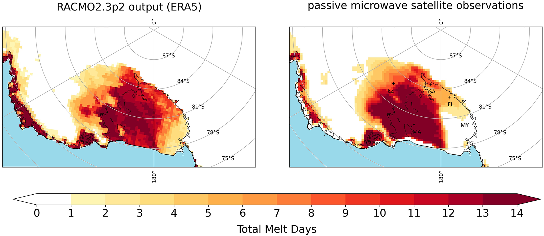
As stated before, Antarctic climatological melt simulated by RACMO2.3p2 has been evaluated extensively (step 1). Here, we add a well-documented case study to the previous work, the January 2016 melt event over the Ross Ice Shelf. For the melt event over the RIS, RACMO2.3p2 produces a geographical distribution of melt days that largely overlaps with the passive microwave satellite observations (Fig. 1). The RACMO2.3p2 output has a relatively small positive bias, meaning that the RACMO2.3p2 output covers an area 5.8% larger compared to the satellite-measured melt area, which corresponds to an area of 41 553 km2. This increased melt area in the RACMO2.3p2 data is especially noticeable in the western sector of the RIS, and also persists in some areas for up to 9 days. The melt day density (total of melt days summed across melt area) is higher in the satellite observations, with RACMO2.3p2 exhibiting a negative bias and showing a melt day density that is 4.1% lower than observed (with 398 fewer total melt days compared to the 9611 detected in the satellite data). In the eastern part of the RIS, the focal point of the melt event, the density of melt days is higher in the satellite observations. In contrast, the melt appears more extensive in RACMO2.3p2 along the ice shelves of Mary Byrd Land. Lastly, RACMO2.3p2 captures spatial variability well, as evidenced by the reduced number of melt days over Roosevelt Island and Siple Dome, which lay at higher elevations.
Map of West Antarctica showing the distribution of total melt days in January 2016 according to daily RACMO2.3p2 (ERA5) output (left side) and according to passive microwave satellite observations (right side). The dataset for the melt day data was provided by Picard and others Reference Picard, Fily and Gallee(2007) and data processing is detailed in the methodology section. Locations of the AWS (EL: Elaine, EZ: Elizabeth, MY: Marilyn, MA: Margaret, SA: Sabrina) analysed are shown on the right map.

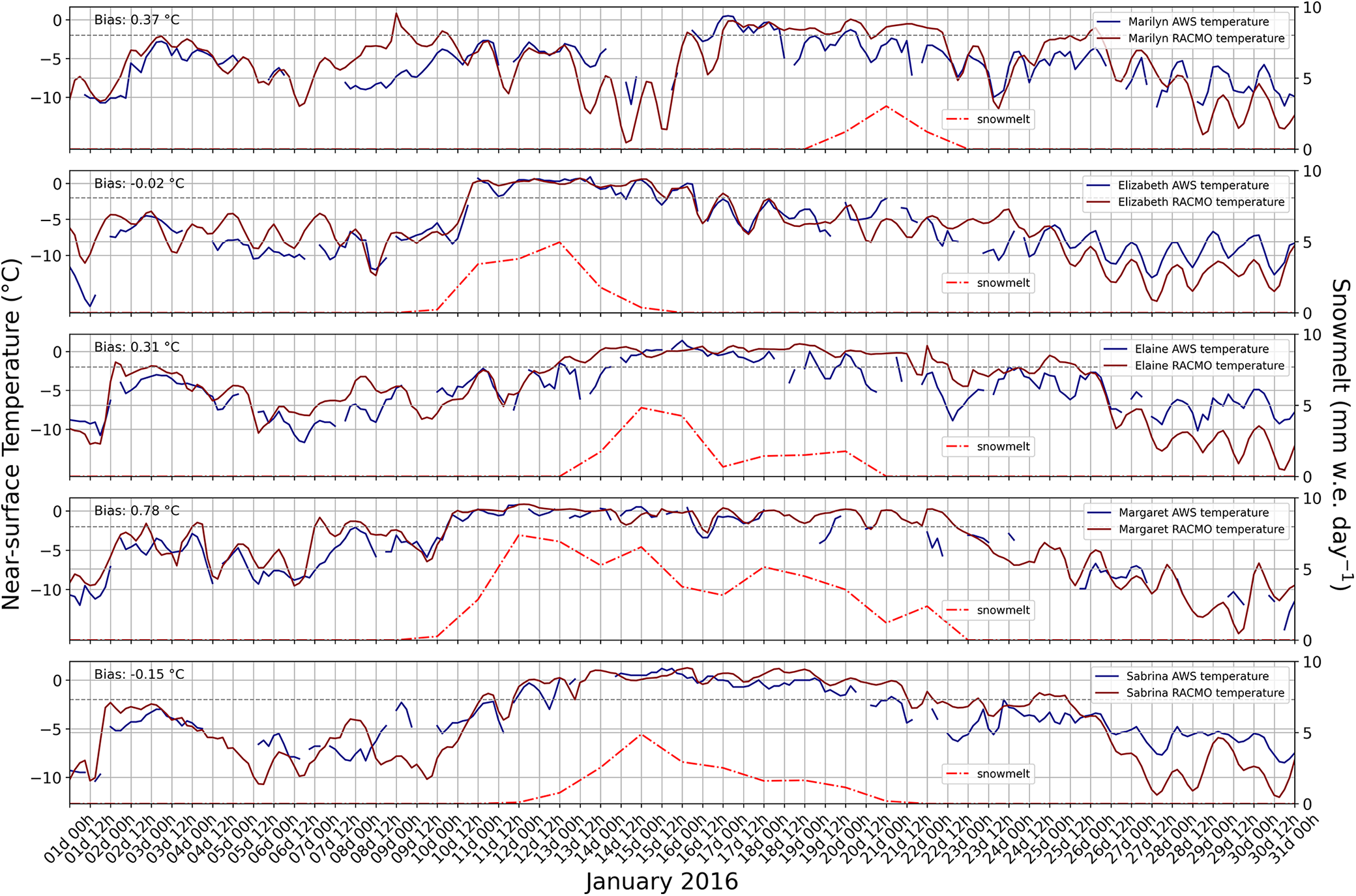
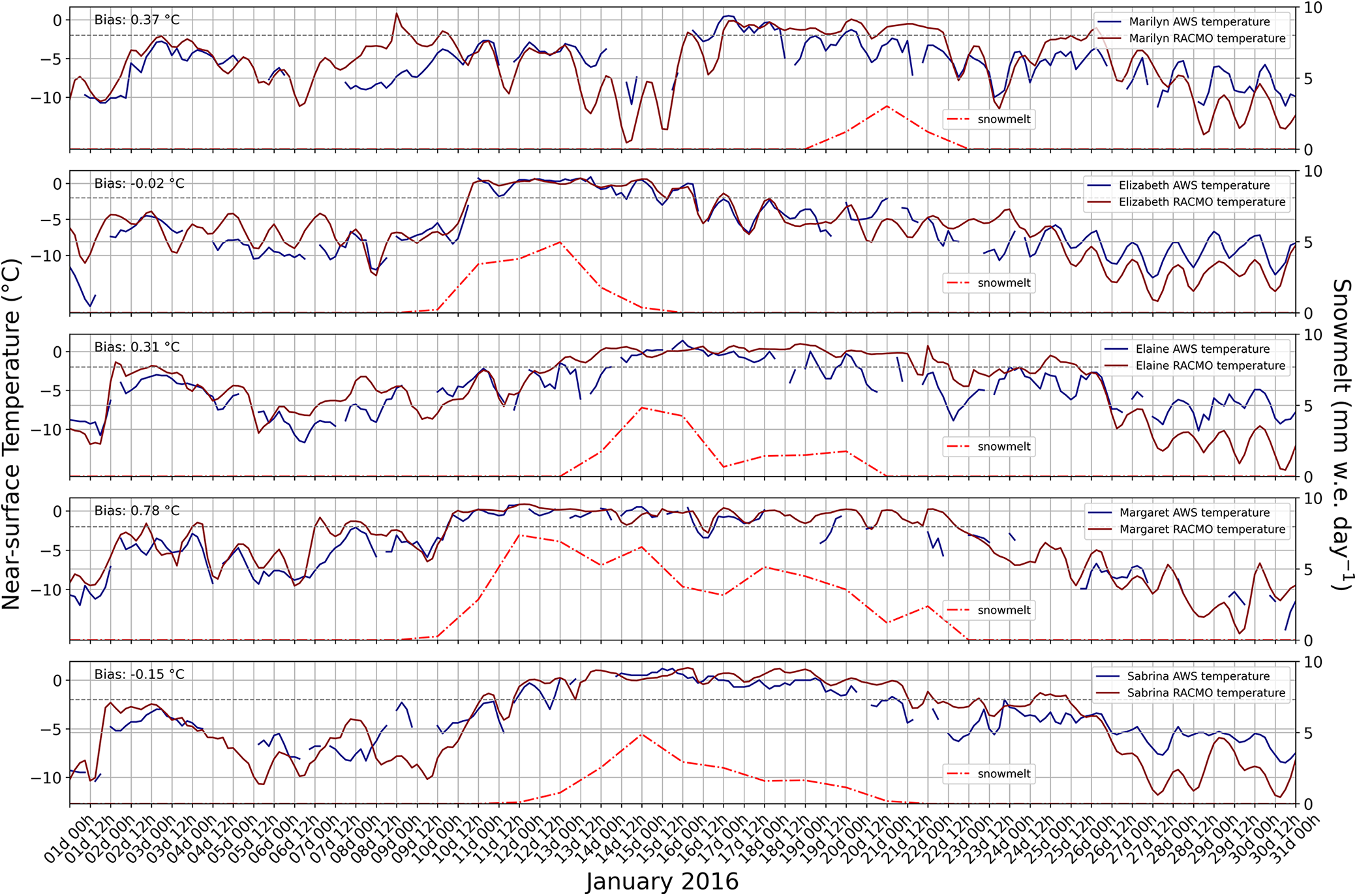
A relevant comparison for melt occurrence and melt rate between model output and in-situ observational data is near-surface temperature. Figure 2 compares 3-hourly RACMO2.3p2 outputs alongside data from five automatic weather stations. At Marilyn AWS, the westernmost station, RACMO2.3p2 predicts six days with temperatures above the melt threshold of -2∘C used by Nicolas and others Reference Nicolas(2017). However, observational data only recorded two such days, corresponding to minimal surface melt, as also indicated by the satellite data (Fig. 2). The higher RACMO2.3p2 temperatures in the western sector of the RIS explain the higher melt day density in this region, which is indicated by positive bias values for both Marilyn and Elaine AWS located in the western part (Fig. 2). Measured near-surface temperatures indicate that the melt event in the western RIS started later, peaking on 2016-01-22, whereas at Elizabeth AWS, the easternmost station, melting started on 2016-01-10. Stations near the Transantarctic Mountains, Elaine and Sabrina AWS, recorded a peak in air temperature well above the freezing point on January 15, following a sharp rise in near-surface temperatures, which remained around or above 0∘C for about six days, leading to prolonged snowmelt. This pattern holds for both observational and modelled temperatures. Notably, the longest melt duration occurred at Margaret station, located north of the RIS near Roosevelt Island, where both satellite and RACMO2.3p2 data indicate a melt period of up to 14 days. At Margaret station RACMO2.3p2 temperatures also have a stronger positive bias of 0.8∘C. Despite some discrepancies in the western RIS and at Margaret AWS, near-surface temperatures from RACMO2.3p2 generally align well with observational data as indicated by the low bias values (Fig. 2). Adding this result to previous melt evaluations of RACMO2.3p2 forced by ERA5 (van Wessem and others, Reference van Wessem2018, Reference van Wessem, van den Broeke, Wouters and Lhermitte2023; Jakobs and others, Reference Jakobs, Reijmer, Smeets, Trusel, van de Berg, van den Broeke and van Wessem2020; Noël and others, Reference Noël, van Wessem and Wouters2023) we conclude that the first evaluation step is passed and that the modelled melt during the historical period is robust.
Time series of 2-metre temperature (in ∘C) from 2016-01-01 to 2016-01-31 at selected AWS in the Ross Ice Shelf. Dark red line shows 3-hourly resolution RACMO2.3p2 output forced by ERA5. Darkblue line shows 3-hourly resolution observational AWS data provided by Wang and others Reference Wang(2023). Bias values between the RACMO2.3p2 and the AWS temperatures are given in the upper left corner. Missing data points in the AntAWS dataset are reflected as discontinuities in the line graphs. The grey horizontal dotted line indicates a temperature of -2∘C, which has been suggested as the event’s melting threshold by Nicolas and others Reference Nicolas(2017). The bright red dash-dot line indicates the magnitude of snowmelt in mm w.e. per day according to RACMO2.3p2 throughout the month of January.
3.2. Step 2: Evaluation of ERA5 vs. CESM2 atmospheric forcing
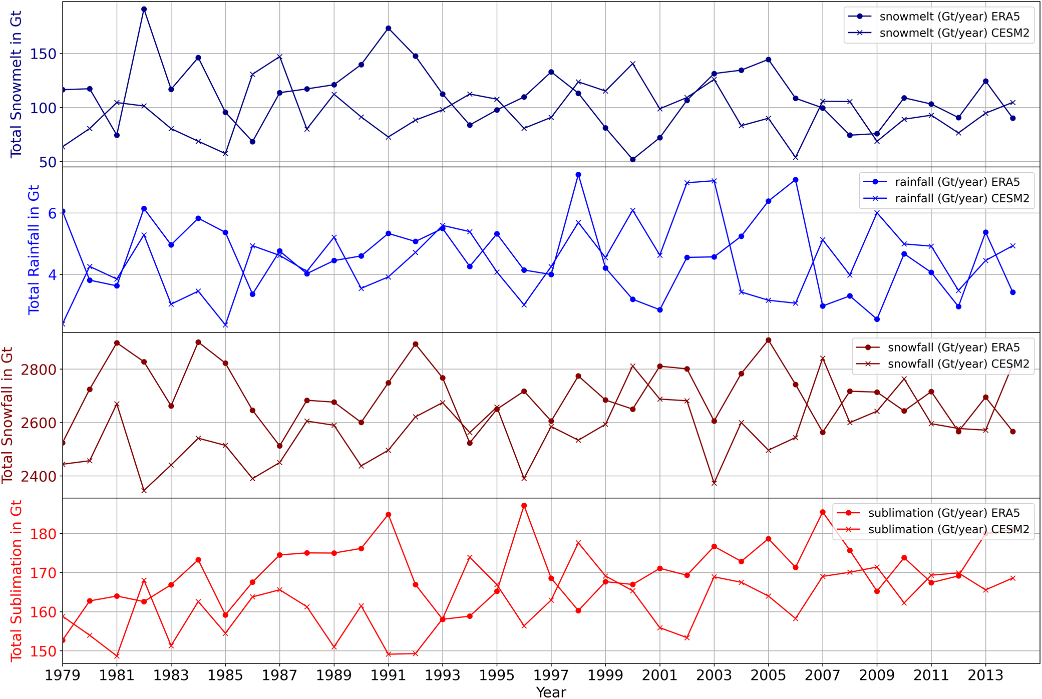
To evaluate the accuracy of the CESM2 forcing on RACMO2.3p2, a comparative time series analysis was conducted using both ERA5 and CESM2 forced runs (Fig. 3) to see whether mean and variability are comparable. The mean and annual variability of the components relevant to the MoA largely coincide (Table 1). For snowfall, CESM2 generally predicts slightly lower mean values, but exhibits higher variability than ERA5 (Table 1). CESM2 shows a small positive trend (6.02 Gt year−2) of the annual snowfall flux, while this is not observed in the ERA5 data. Both ERA5 and CESM2 indicate a minor positive trend in sublimation rates from 1979 to 2014. The linear regression revealed that for all other fluxes the slope is not significantly different from zero.
Total AIS (grounded ice sheet including ice shelves) integrated fluxes that contribute to either liquid water presence or accumulation at the ice surface in gigatonnes per year from 1979 to 2014. Average values, standard deviation and trend are given in Table 1. Absolute values are shown. See the methodology section for detailed information on data processing.
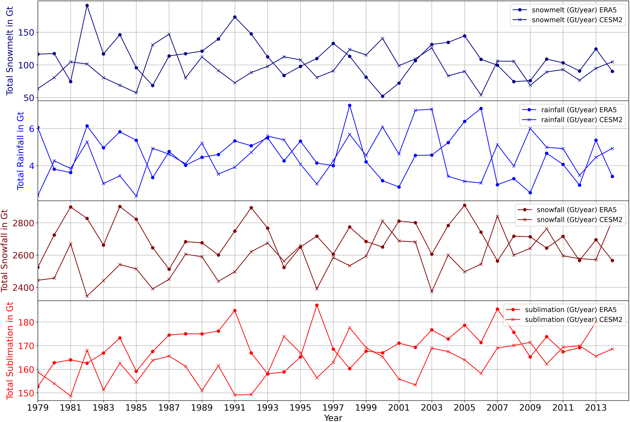
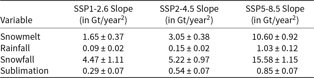
Mean and standard deviation (variability) of total annual fluxes of MoA (snowmelt, rainfall, snowfall and sublimation) for ERA5 and CESM2 forcings (1979–2014). Alongside slope for linear regression line and uncertainty of the slope parameter. The standard deviation and variability are computed over time for spatially-integrated variables

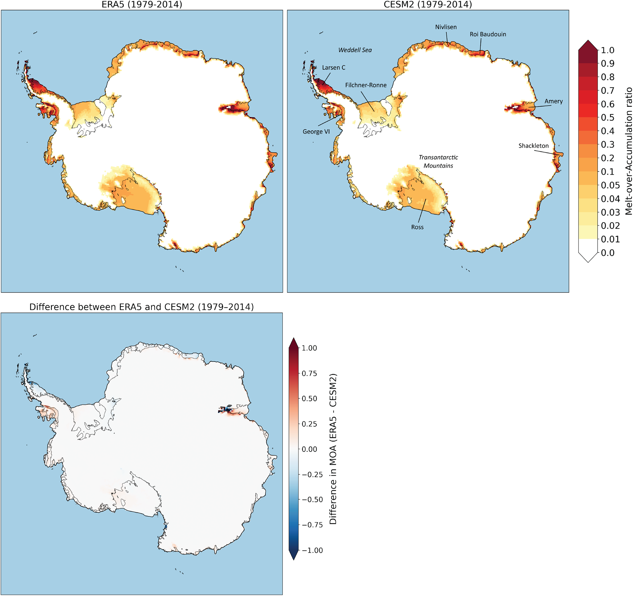
ERA5 and CESM2 revealed a consistent geographical distribution of MoA ratios (Fig. 4). The geographical distribution of MoA is consistent between the two (Fig. 4), with CESM2 showing slightly lower MoA ratios near the Antarctic Peninsula and Amery Ice Shelf, but higher values on the eastern Filchner-Ronne Ice Shelf, which extend further into the ice shelf’s interior. This is most likely partly associated with the lower resolution of CESM2 forcing.
Melt-over-accumulation ratio between 1979 to 2014 from RACMO2.3p2 with ERA5 (top left) and CESM2 (top right) forcing. The difference between ERA5 and CESM2 forcing is given in bottom left panel, with hatching denoting areas where the differences exceed interannual variability. Note the non-linear scale.
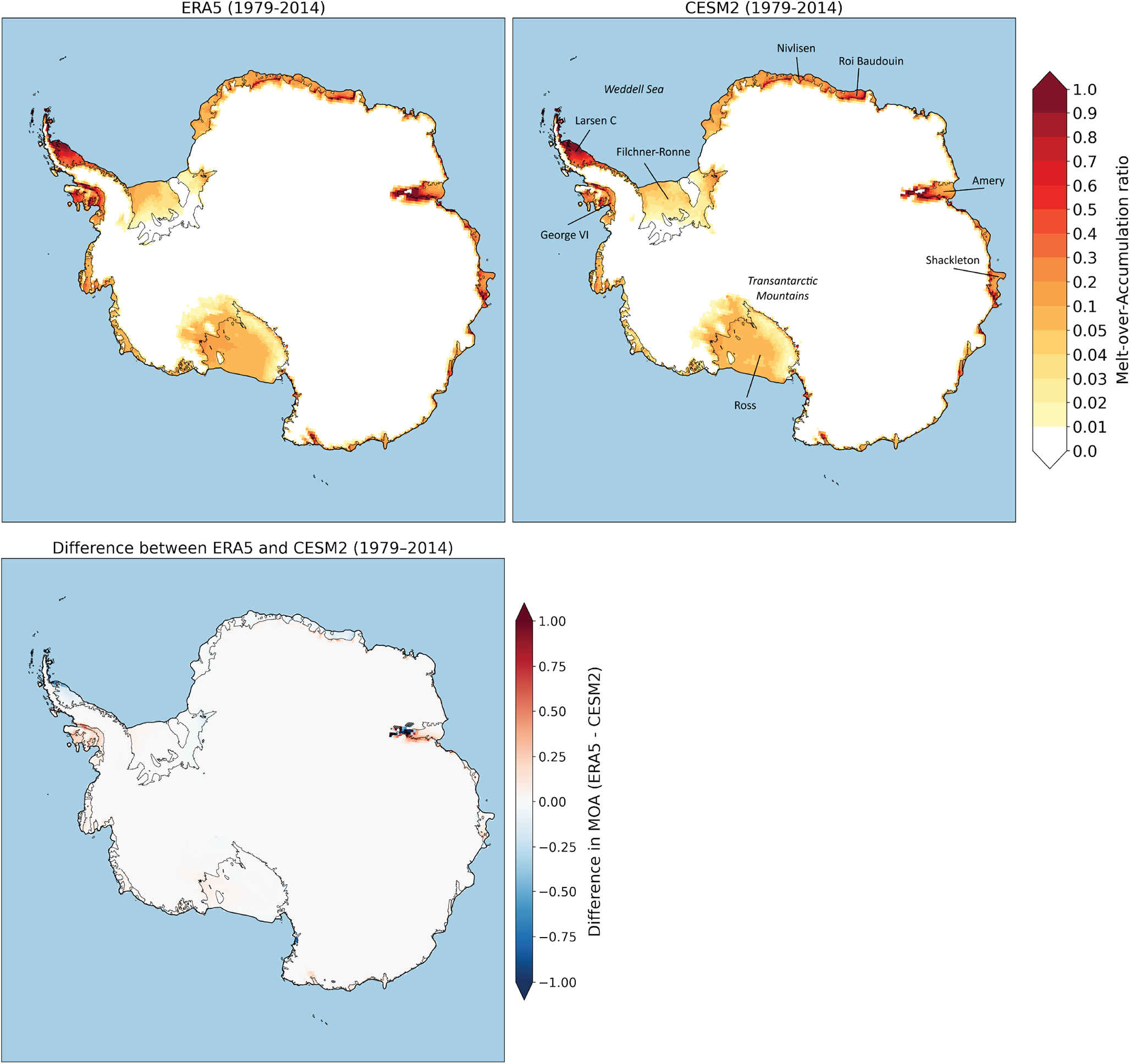
The highest MoA values (up to 1.0) are found on the Antarctic Peninsula, particularly along the coast of the Larsen C Ice Shelf, and at the grounding line of the Roi Baudouin and Amery Ice Shelves in East Antarctica (Fig. 4). This also correlates with observations of melt ponding on these ice shelves (Luckman and others, Reference Luckman, Elvidge, Jansen, Kulessa, Munneke, King and Barrand2014; Lenaerts and others, Reference Lenaerts2017). The major ice shelves like Filchner-Ronne and Ross exhibit only low MoA values (up to 0.04) (Fig. 4). Negative MoA values are found near the intersection of the Lambert and Fisher glaciers with the Amery Ice Shelf, where sublimation exceeds precipitation, hence indicating ablation, i.e. a blue-ice zone (shown as white 0 values in Fig. 4). Thus, a ratio of MoA is not meaningful for this area as these results suggest that there is no firn layer present.
The difference between both simulated MoA values is only found to exceed the interannual variability near the grounding line of the Amery ice shelf (Fig. 4). The comparable annual mean, inter-annual variability and geographical distribution between both simulations mean that evaluation step 2 is passed, which supports the reliability of RACMO2.3p2 for future projections when forced by CESM2.
3.3. Application: Future MoA
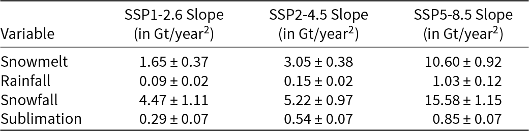
Now that the robustness of CESM2 forced RACMO2.3p2 for MoA has been established based on the two-step evaluation procedure, we present future results as a first application. A linear regression was performed on the time series of each of the components of MoA for all three emission scenarios, which show that accumulation rates and liquid water availability at the ice sheet surface increase across all emission scenarios (Table 2). Specifically, snowfall mass flux increases by about 4.5, 5.2, and 15.6 Gt year-2 in the SSP1-2.6, SSP2-4.5, and SSP5-8.5 scenarios, respectively (Table 2). Correspondingly, the total surface melt flux increases by approximately 1.7, 3.1, and 10.6 Gt year-2 under the SSP1-2.6, SSP2-4.5, and SSP5-8.5 scenarios (Table 2). The trend in liquid precipitation shows the most substantial increase under the SSP5-8.5 scenario, reaching 1.0 Gt year-2, compared to 0.1 and 0.2 Gt year-2 for scenarios SSP1-2.6 and SSP2-4.5, respectively.
Results of linear regression analysis: slope (in Gt year-2) and uncertainty of the slope parameter for total annual amounts under scenarios SSP1-2.6, SSP2-4.5 and SSP5-8.5
In all SSP scenarios, the MoA ratio remains zero across the interior of the Antarctic Ice Sheet, where extremely low temperatures prevent any surface melt from occurring.
This trend holds across all projection runs, despite varying extents to which positive MoA values extended into the interior.
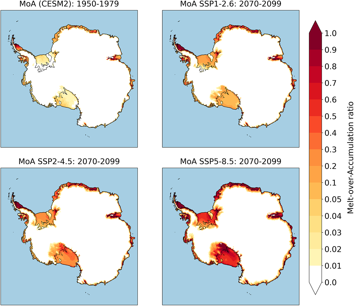
Under the SSP1-2.6 scenario, an increase in MoA is observed across all ice shelves by the end of the century. Notably, the Larsen C, George VI, Roi Baudouin, Amery, and parts of the Shackleton Ice Shelves exhibit higher MoA values (0.5–1.0) compared to pre-20th century levels (Fig. 5). The largest absolute changes are seen on the Larsen C Ice Shelf and near the grounding line of the Roi Baudouin Ice Shelf, with increases of about 0.75–1.0.
Melt-over-accumulation ratio before the start of the century (1950–79) and at the end of the century (2070–99) under three emission scenarios.
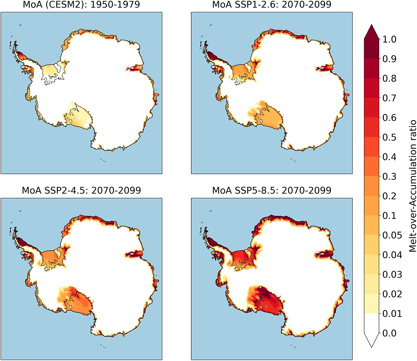
Under the SSP2-4.5 scenario, the MoA values are similar to those of the low-emissions scenario, only slightly higher. Most grid cells on the Larsen C Ice Shelf reach a MoA value over 1.0 (Fig. 5). East of the Filchner-Ronne, MoA values (0.3-0.6) are higher, as well as south of the RIS (at the lee side of the Transantarctic Mountains), than under SSP1-2.6. On these major ice shelves, MoA changes at a range between 0.05 and 0.5 (Fig. 5).
Under the SSP5-8.5 scenario, the most pronounced changes are observed, where all ice shelves at least partly exceed the MoA threshold of 0.7 (Fig. 5). MoA values above 1.0 are found on the ice shelves of the Antarctic Peninsula, Nivlisen, Roi Baudouin, and around the Shackleton Ice Shelf (Fig. 5). The Filchner-Ronne and Ross Ice Shelves also experience substantial increases in MoA, with values ranging from 0.3 to 1.0. Here, absolute changes up to 0.75 in MoA occur by the end of the century, compared to pre-21st century levels. Various ice shelves along the West Antarctic Ice Sheet and the Weddell Sea coast show much higher MoA values (up to 1.0). This confirms the vulnerability of many Antarctic ice shelves for meltwater ponding in a future warming scenario (van Wessem and others, Reference van Wessem, van den Broeke, Wouters and Lhermitte2023).
4. Discussion
4.1. Two-step evaluation
Here, given extensive previous work, only a limited additional evaluation of RACMO2.3p2/ERA5 for AIS melt was performed. As shown by the limited biases, the analysis of the January 2016 surface melt event over the Ross sector indicates that the RACMO2.3p2 melt product is realistic and aligns well with observational data (step 1). This is evident as temporal and spatial patterns align with passive microwave observations and AWS data. This confirms the reliability of RACMO2.3p2’s surface melt product in the contemporary climate (step 1).
In evaluation step 2, RACMO2.3p2 forced by CESM2 accurately identifies regions with elevated MoA ratios. Its spatial distribution of MoA closely aligns with the ERA5 forced run (step 2).
These results demonstrate the added value of the two-step procedure to put more confidence in the future projection results.
4.2. Application: Future melt-over-accumulation ratios
After evaluation, the predicted MoA values were presented and discussed. MoA is very relevant for future AIS mass balance loss, because both solid and liquid input are expected to change and impact the viability of Antarctic ice shelves. Snow accumulation is projected to increase approximately linearly with temperature, although this trend exhibits regional differences (Palerme and others, Reference Palerme, Genthon, Claud, Kay, Wood and L’Ecuyer2017; van Wessem and others, Reference van Wessem, van den Broeke, Wouters and Lhermitte2023). The high-emission scenario predicts crucial changes in precipitation phase with a nearly 10-fold increase in the annual rainfall rate between the low and high emission scenario, increasing the liquid-to-solid precipitation ratio (Table 2). The phase of precipitation matters strongly for the ice shelves: snow increases albedo and contributes to firn pore space, while rain lowers the albedo and further consumes pore space (van Wessem and others, Reference van Wessem, van den Broeke, Wouters and Lhermitte2023). The change in precipitation phase will likely be most pronounced on local scales (Vignon and others, Reference Vignon, Roussel, Gorodetskaya, Genthon and Berne2021). Simultaneously, surface melt is projected to increase more sharply than snow accumulation with rising temperatures due to feedback mechanisms (Trusel and others, Reference Trusel2015), the strongest being the snowmelt-albedo feedback (Jakobs and others, Reference Jakobs, Reijmer, Kuipers Munneke, König-Langlo and van den Broeke2019).
In particular, the large difference between SSP1-2.6 and SSP2-4.5 scenarios on one hand and the high emission scenario (SSP5-8.5) on the other, could be attributed to the increase in solid precipitation, thereby mitigating surface melt for modest warming. The mitigation primarily results from the influence of surface melt waters on albedo; and as new snow accumulates, it brightens the surface, reducing melt. In the high-emission SSP5-8.5 scenario, however, the ratio between surface melt and snow accumulation is larger (0.37 for SSP1-2.6, 0.58 for SSP2-4.5 and 0.68 for SSP5-8.5), indicating that surface melt is less counterbalanced by increased snowfall, as the melt-albedo mechanism overtakes. These trends make the ice shelves under strong warming particularly vulnerable to melt ponding and hydrofracturing.
5. Conclusions
We make the case for a two-step evaluation procedure before using regional climate models (RCMs) for future projection, e.g. of ice sheet mass balance. In this study, RACMO2.3p2 forced by the ERA5 reanalysis and by the CESM2 Earth System Model for the Antarctic ice sheet are given as an example of such a procedure. The analysis of the well-documented 2016 melt event over the Ross Ice Shelf, together with previous evaluations, revealed that RACMO2.3p2 is a robust regional climate model for quantifying surface melt over Antarctica when forced with ERA5 (step 1). Further, RACMO2.3p2 forced by ERA5 and CESM2 show a strong agreement in simulated MoA during the historical period, both for annual statistics as for spatial variability (step 2).
Based on the satisfactory two-step evaluation procedure, we present and analyse three future realizations of Antarctic climate and their respective geographically-distributed MoA values. The MoA threshold of 0.7, which indicates the potential for persistent surface melt and meltwater ponding, is only reached on the Larsen C and Roi Baudouin ice shelves under the SSP1-2.6 and SSP2-4.5 scenarios. The SSP5-8.5 scenario projects that numerous grid cells across a majority of the ice shelves will surpass this value. The two-step evaluation process increases confidence in these results.
Acknowledgements
We acknowledge funding from the Netherlands Earth System Science Centre (NESSC) and the European Union’s Horizon 2020 research and innovation programme Marie Skłodowska-Curie, grant agreement No. 847504. MvdB is supported by EMBRACER (Summit grant SUMMIT.1.034) financed by the Netherlands Organisation for Scientific Research (NWO) and the Netherlands Earth System Science Center (NESSC) financed by the Dutch Ministry of Education, Culture and Science.


 Open access

