


1. Introduction
The convective flows resulting from uniform vertical buoyancy sources, which we term ‘distributed wall-source plumes’, occur widely within both geophysical environments and within the built environment. Examples include the dissolution of a wall of ice dissolving into seawater (McConnochie & Kerr Reference McConnochie and Kerr2015) and the downdraught resulting from a relatively cold flow from a glazed façade within a building in winter (Heiselberg Reference Heiselberg1994) or, similarly, any heated vertical surface within a building, be it from a radiator or from incident solar radiation. In these contexts the resulting distributed wall-source plumes are usually turbulent. We carry out simultaneous high-resolution experimental measurements of the velocity and buoyancy fields of turbulent distributed wall-source plumes in order to investigate the structure of the plume and the resulting entrainment of ambient fluid.
With increasing vertical distance along the wall these initially laminar convective flows become unstable and transition to turbulence. Turbulent distributed wall-source plumes are comprised of three distinct layers: a viscous sub-layer, a viscous–turbulent overlap layer and an outer inertial turbulent layer (Holling & Herwig Reference Holling and Herwig2005). In most cases of relevance, the flows will become fully turbulent due to the large vertical extent and sufficiently large buoyancy flux of the source. The transition to turbulence for an isothermal wall may be characterised by the Grashof number
 \begin{equation} Gr=\frac{g\beta {\rm \Delta} T z^3}{\nu^2}, \end{equation}
where  $g$ is the acceleration due to gravity, $\beta$ is the thermal expansion coefficient, ${\rm \Delta} T$ is the temperature difference between the wall and the ambient, $\nu$ is the kinematic viscosity of the fluid and $z$ is the vertical distance along the wall. The transition to turbulence occurs at approximately $Gr=10^9$ (Bejan & Lage Reference Bejan and Lage1990). This implies, for example, that the transition to turbulence of an isothermal heated wall in a room with ${\rm \Delta} T=10\ \textrm {K}$ would occur at $z\approx {0.5}\ \textrm {m}$. Considering the typical vertical extent of internal spaces within buildings, $H\sim {10}\ \textrm {m}$, it is reasonable to assume that the plume over the majority of the height of the wall is turbulent. Josberger & Martin (Reference Josberger and Martin1981) studied the melting of a vertical ice sheet in typical oceanic salinities ( ${\sim }3$ wt% NaCl) and found that for ambient temperatures in the range $0$ to $20\,^{\circ }\textrm {C}$ the flow transitions to turbulence at heights of $0.10\text {--}{0.30}\ \textrm {m}$. This may be compared to the typical vertical extent of icebergs in the North Atlantic of 100 m or in the Antarctic of 250 m.
The primary aim of the early studies on natural convection was to determine the velocity and temperature profiles and calculate the rate of turbulent heat transfer in both the laminar and turbulent regimes (Batchelor Reference Batchelor1954; Nachtsheim Reference Nachtsheim1963; Vliet & Liu Reference Vliet and Liu1969). While the laminar flow is well understood (Ostrach Reference Ostrach1953; Kuiken Reference Kuiken1968), there is no formal theoretical solution for turbulent flow (Wells & Worster Reference Wells and Worster2008). The evolution of the heat flux  $q^{\prime \prime }(z)$ with height is typically represented in terms of the Nusselt number,
 \begin{equation} Nu=\frac{q^{\prime\prime}(z)z}{\rho c_p \kappa {\rm \Delta} T}, \end{equation}
where  $c_p$ is the specific heat capacity, $\kappa$ is the thermal diffusivity and $\rho$ is the density of the fluid. Experimental investigations of an isothermal wall in air of differing temperature (e.g. Cheesewright Reference Cheesewright1968; Pirovano, Viannay & Jannot Reference Pirovano, Viannay and Jannot1970; Tsuji & Nagano Reference Tsuji and Nagano1988) have shown that in the turbulent region of the flow
 \begin{equation} Nu\sim Ra^{r}, \end{equation}
where  $Ra=GrPr$ is the Rayleigh number, $Pr = \nu /\kappa$ is the Prandtl number and $r\approx 1/3$. Given that the Prandtl number is a property of the fluid and therefore invariant with height, substituting (1.1) and (1.2) into (1.3) suggests that the heat flux is invariant with height within the turbulent regime of an isothermally heated or cooled wall and, following Batchelor (Reference Batchelor1954), the heat flux per unit area may be characterised by the buoyancy flux per unit area
 \begin{equation} f=\frac{g\beta q''}{\rho c_p}. \end{equation}
So that, although the boundary conditions differ in the two flows, an approximately statistical equivalence exists between the turbulent region of an isothermal wall and a uniform vertically distributed buoyancy source.
Following the framework of Morton, Taylor & Turner (Reference Morton, Taylor and Turner1956), Wells & Worster (Reference Wells and Worster2008) and Cooper & Hunt (Reference Cooper and Hunt2010) modelled the flow resulting from a uniform vertically distributed wall-source buoyancy flux by using an entrainment coefficient to parameterise the mixing of the plume with the ambient fluid. Cooper & Hunt (Reference Cooper and Hunt2010) tested the model experimentally by forcing relatively dense salt solution through a porous wall into fresh water to produce the distributed buoyancy source. There have since been numerous investigations of vertically distributed buoyancy sources applying the plume theory developed by Cooper & Hunt (Reference Cooper and Hunt2010). A direct numerical simulation study by Gayen, Griffiths & Kerr (Reference Gayen, Griffiths and Kerr2016) replicated experiments by McConnochie & Kerr (Reference McConnochie and Kerr2015), who used an ice block adjacent to fresh water to create a vertically distributed source. The results showed good agreement between the predicted bulk flux scalings of Cooper & Hunt (Reference Cooper and Hunt2010). Caudwell, Flór & Negretti (Reference Caudwell, Flór and Negretti2016) performed velocity and temperature measurements on a heated wall placed in water and Bonnebaigt, Caulfield & Linden (Reference Bonnebaigt, Caulfield and Linden2018) approximated a uniformly distributed buoyancy source by using discrete point sources of salt water distributed throughout a vertical wall. In order to match the model with the experimental results a value of the entrainment coefficient  $\alpha$, which is the ratio of the entrainment velocity (i.e. the velocity at which ambient fluid enters the plume) to the vertical velocity in the plume, is needed. The studies mentioned above have found it necessary to use significantly different values of $\alpha$ to obtain agreement.
In a confined environment the plume establishes a ‘filling box’ flow (Baines & Turner Reference Baines and Turner1969) in a which a stable stratification is established behind a moving horizontal ‘first front’ which demarcates the initial unstratified ambient from the developing stratified region behind the front. By measuring the velocity of this first front it is possible to estimate the entrainment coefficient (Baines Reference Baines1983). Using this method Cooper & Hunt (Reference Cooper and Hunt2010) and Bonnebaigt et al. (Reference Bonnebaigt, Caulfield and Linden2018) found relatively small values of the entrainment coefficient  $\alpha =0.02$ and $\alpha =0.018$, respectively. McConnochie & Kerr (Reference McConnochie and Kerr2015) also used the filling box method in order to determine the entrainment coefficient. By accounting for the wall shear stress they found a larger entrainment coefficient of $\alpha =0.048$. Gayen et al. (Reference Gayen, Griffiths and Kerr2016) and Caudwell et al. (Reference Caudwell, Flór and Negretti2016) calculated the entrainment coefficient directly from velocity data and found even higher values of $\alpha =0.059$ and $\alpha =0.08$, respectively. Kaye & Cooper (Reference Kaye and Cooper2018) have partially explained the discrepancies between these studies by accounting for the wall shear stress and the volume flux of fluid injected at the wall not considered in Cooper & Hunt (Reference Cooper and Hunt2010) and Bonnebaigt et al. (Reference Bonnebaigt, Caulfield and Linden2018). Nevertheless, given the difficulty in both creating a truly uniform distributed buoyancy source and performing accurate velocity measurements of the distributed wall-source plume it is, perhaps, understandable as to why there is not more agreement between these studies, especially since they used different methods to create the distributed buoyancy source and measure the resulting flow. One of the main aims of this paper is to resolve such discrepancies by carrying out high fidelity experimental measurements and a robust analysis of the data examining the mixing via two different methods for calculating values of the entrainment coefficient for a distributed wall-source plume. The work is divided into two parts. In this first part we consider the distributed wall-source plume in an unconfined unstratified environment. In Part 2 (Parker et al. Reference Parker, Burridge, Partridge, Hacker and Linden2021), we consider the distributed wall-source plume in a both an unventilated confined (filling box) environment, and use the results obtained in this part to improve the peeling model originally developed by Bonnebaigt et al. (Reference Bonnebaigt, Caulfield and Linden2018), and a ventilated confined (emptying filling box) environment. This part is organised as follows. We review plume theory for distributed wall plumes in § 2 and extend the numerical investigation of the finite-flux plume equations described by Kaye & Cooper (Reference Kaye and Cooper2018) to include a finite wall shear stress. The experimental methods are described in § 3. The results of the velocity measurements examining the whole height of the wall are presented in § 4.1 and the simultaneous velocity and buoyancy measurements examining the turbulent and self-similar region are presented in § 4.2. Finally, conclusions are drawn in § 5.
2. Theory
Here we outline the theory for vertically distributed turbulent plumes produced by a uniform and constant buoyancy flux imposed at a vertical wall in an unstratified quiescent infinite environment. We consider the case of both an ideal buoyancy source, where buoyancy diffuses from the boundary with no source volume flux, and a buoyancy source with a finite source volume flux. We denote the velocity  $w(x,z,t)$ in the vertical $z$-direction, horizontal velocity $u(x,z,t)$ in the across-plume $x$-direction, the deviation from hydrostatic pressure $p(x,z,t)$ and the buoyancy $b(x,z,t)=g(\rho _a-\rho (x,z,t))/\rho _a$, where $\rho$ and $\rho _a$ are the density of the plume and ambient fluid, respectively, and we assume that $\rho _a-\rho \ll \rho _a$ so that the Boussinesq approximation applies, as it does in the practical cases discussed in § 1. Since the flow is statistically steady, these quantities may be decomposed into time-averaged and fluctuating components $w(x,z,t)=\bar {w}(x,z)+w'(x,z,t)$, $u(x,z,t)=\bar {u}(x,z)+u'(x,z,t)$ and $b(x,z,t)=\bar {b}(x,z)+b'(x,z,t)$, and we denote the time-averaged maximum vertical velocity as $\bar {w}_m(z)$. The coordinate system is defined so that the wall is at $x=0$. We assume all quantities are independent of the along-wall horizontal $y$-direction. We define the time-averaged volume flux, specific momentum flux, integral buoyancy and buoyancy flux per unit length by
 \begin{gather} Q_p(z)=\int_{0}^{\infty}\bar{w}(x,z) \,\mathrm{d} x, \end{gather}
 \begin{gather}M(z)=\int_{0}^{\infty}\bar{w}^2(x,z) \,\mathrm{d} x, \end{gather}
 \begin{gather}B(z)=\int_{0}^{\infty}\bar{b}(x,z) \,\mathrm{d} x, \end{gather}
 \begin{gather}F(z)=\int_{0}^{\infty}\bar{w}(x,z)\bar{b}(x,z)+\overline{w'(x,z,t)b'(x,z,t)} \,\mathrm{d} x. \end{gather}
From these relations we define the characteristic scales for plume width  $R$, velocity $W$ and buoyancy $b_T$ by
 \begin{gather} R=\frac{Q_p^2}{M}, \end{gather}
 \begin{gather}W=\frac{M}{Q_p}, \end{gather}
 \begin{gather}b_T=\frac{F}{Q_p}. \end{gather}
Under the Boussinesq approximation and by employing the boundary layer approximation, the Reynolds time-averaged mass, vertical momentum and buoyancy conservation equations may be written, respectively, as
 \begin{gather} \frac{\partial \bar{u}}{\partial x}+\frac{\partial \bar{w}}{\partial z}=0, \end{gather}
 \begin{gather}\bar{u}\frac{\partial \bar{w}}{\partial x}+\bar{w}\frac{\partial \bar{w}}{\partial z}+\frac{\partial \overline{w'^2}}{\partial z}+\frac{\partial\overline{u'w'}}{\partial x}=-\frac{1}{\rho_a}\frac{\partial \bar{p}}{\partial z}+\bar{b} +\nu \frac{\partial^2 \bar{w}}{\partial x^2}, \end{gather}
 \begin{gather}\bar{u}\frac{\partial \bar{b}}{\partial x}+\bar{w}\frac{\partial \bar{b}}{\partial z}+\frac{\partial\overline{u'b'}}{\partial x}+\frac{\partial\overline{w'b'}}{\partial z}=\kappa \frac{\partial^2 \bar{b}}{\partial x^2}, \end{gather}
where  $\nu$ and $\kappa$ are the kinematic viscosity of the fluid and diffusivity of the scalar responsible for the buoyancy, respectively. Integration of (2.8)–(2.10) with respect to $x$ gives
 \begin{gather} \frac{\mathrm{d} Q_p}{\mathrm{d} z}=-\left.\bar{u}\right|_0^{\infty}, \end{gather}
 \begin{gather}\frac{\mathrm{d} M}{\mathrm{d} z}+\left.\left[\overline{uw}+\overline{u'w'}\right]\right|_{0}^{\infty}= B-\frac{\mathrm{d}}{\mathrm{d} z}\left(\int_{0}^{\infty}\overline{w'^2}+\frac{1}{\rho_a}\frac{\partial \bar{p}}{\partial z} \,\mathrm{d} x\right)+\left.\nu\frac{\partial \bar{w}}{\partial x}\right|_{0}^{\infty}, \end{gather}
 \begin{gather}\frac{\mathrm{d} F}{\mathrm{d} z}+\left.\overline{u'b'}\right|_{0}^{\infty}=\left.\kappa\frac{\partial \bar{b}}{\partial x}\right|_{0}^{\infty}. \end{gather}
Under the entrainment assumption, the inflow velocity of ambient fluid at any height is proportional to the local average vertical plume velocity i.e.  $-\bar {u}(\infty ,z)=\alpha W$, where $\alpha$ is the integral entrainment coefficient which, with this averaging procedure, is equal to the ‘top-hat’ entrainment coefficient (Morton et al. Reference Morton, Taylor and Turner1956). Using the boundary conditions $\bar {w}(0,z)= \overline {u'w'} (0,z) = \overline {u'b'} (0,z) = \bar {w}(\infty ,z) = \overline {u'w'} (\infty ,z) = \overline {u'b'} (\infty ,z) = 0$, $\bar {u}(0,z)=q$ and ${\partial b}/{\partial x}|_{0}=f/\kappa$, the Boussinesq time-averaged volume, momentum and buoyancy flux conservation equations may be written as (Kaye & Cooper Reference Kaye and Cooper2018)
 \begin{gather} \frac{\mathrm{d} Q_p}{\mathrm{d} z}= \alpha\frac{M}{Q_p}+q, \end{gather}
 \begin{gather}\frac{\mathrm{d} M}{\mathrm{d} z}=B-\left.\nu\frac{\partial \bar{w}}{\partial x}\right|_{0}=\frac{\theta F Q_p}{M}-C\left(\frac{M}{Q_p}\right)^2, \end{gather}
 \begin{gather}\frac{\mathrm{d} F}{\mathrm{d} z}=f, \end{gather}
where  $q$ is the additional wall-source volume flux per unit area, and the wall shear stress is expressed in terms of the characteristic velocity $W$ and a constant skin friction coefficient $C$ (Gayen et al. Reference Gayen, Griffiths and Kerr2016). The similarity coefficient $\theta$ is given by
 \begin{equation} \theta = \frac{BM}{FQ_p}, \end{equation}
which in a self-similar plume we may take as a constant.
The contributions from the integral of the velocity fluctuations and pressure term are typically neglected in first-order integral plume models that are based on Morton et al. (Reference Morton, Taylor and Turner1956), i.e. it assumed that
 \begin{equation} \frac{\mathrm{d}}{\mathrm{d} z}\left(\int_{0}^{\infty}\overline{w'^2}+\frac{1}{\rho_a}\frac{\partial \bar{p}}{\partial z}\, \mathrm{d} x\right)\ll \frac{\mathrm{d} M}{\mathrm{d} z}. \end{equation}
This is partially due to fact that the pressure term is extremely difficult to measure experimentally. Experimental studies have verified (2.18) in the case of turbulent momentum-driven two-dimensional flows (Miller & Comings Reference Miller and Comings1957; Bradbury Reference Bradbury1965). Second-order plume integral models typically approximate the pressure by  $\bar {p}\approx (\overline {u'^2}+\overline {v'^2})/2$, where $v$ is the velocity in the $y$-direction. A recent direct numerical simulation study by Van Reeuwijk et al. (Reference Van Reeuwijk, Salizzoni, Hunt and Craske2016) showed the approximation to be valid to within 20 % in an axisymmetric plume. However, measuring the three velocity components simultaneously is challenging and in these experiments we were restricted to measurements of the two velocity components $u$ and $w$ only. We therefore restrict attention to the first-order integral model.
We distinguish between the total plume volume flux  $Q_p$ and the cumulative entrained volume flux defined by
 \begin{equation} Q_e(z)=\int_0^z-\bar{u}(\infty,z') \,\mathrm{d} z'=Q_p-qz. \end{equation}
The solutions to the plume equations (2.14)–(2.16) for a finite volume flux through the wall and no shear stress, i.e.  $q>0$ and $C=0$, were solved numerically by Kaye & Cooper (Reference Kaye and Cooper2018) and compared to the idealised case of zero volume flux through the wall, $q=0$. The ratio of the solutions for the two cases was calculated as a function of the non-dimensional height $\zeta =zf/q^3$, which in all cases monotonically tends to 1 as $z\to \infty$. Hence, for a given wall-source buoyancy flux per unit area $f$ with associated volume flux per unit area $q$, there is a height at which the two solutions are arbitrarily close and the effect of the added volume flux may be neglected. We extend this analysis by numerically solving (2.14)–(2.16) for the case $q>0$ and $C>0$.
We first give the solutions of (2.14)–(2.16), for  $q=0$, in dimensional form (Kaye & Cooper Reference Kaye and Cooper2018),
 \begin{gather} Q_p(z)=\frac{3}{4}\left(\frac{4}{5}\right)^{1/3}\alpha^{2/3}\left(\frac{\theta f}{1+\dfrac{4C}{5\alpha}}\right)^{1/3}z^{4/3}, \end{gather}
 \begin{gather}M(z)=\frac{3}{4}\left(\frac{4}{5}\right)^{2/3}\alpha^{1/3}\left(\frac{\theta f}{1+\dfrac{4C}{5\alpha}}\right)^{2/3}z^{5/3}, \end{gather}
 \begin{gather}F(z)=f z. \end{gather}
From hereon we assume that the similarity coefficient  $\theta =1$ which is justified in § 4.2. For $q>0$ the vertical distance and fluxes of volume, momentum and buoyancy may be non-dimensionalised following Kaye & Cooper (Reference Kaye and Cooper2018) by
 \begin{equation} \zeta=\frac{zf}{q^3},\quad \gamma=\frac{Q_pf}{q^4},\quad \mu=\frac{Mf}{q^5},\quad \phi=\frac{F}{q^3}. \end{equation}
The plume equations (2.14)–(2.16) may then be expressed in non-dimensional form by
 \begin{gather} \frac{\mathrm{d} \gamma}{\mathrm{d} \zeta }=\alpha\frac{\mu}{\gamma}+1, \end{gather}
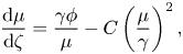 \begin{gather}\frac{\mathrm{d} \mu}{\mathrm{d} \zeta}=\frac{\gamma \phi}{\mu}-C\left(\frac{\mu}{\gamma}\right)^2, \end{gather}
 \begin{gather}\frac{\mathrm{d} \phi}{\mathrm{d} \zeta}=1. \end{gather}
The non-dimensional equations (2.24)–(2.26) were solved numerically over the range  $10^{-4}<\zeta <10^7$ which is equivalent to the range of the experiments performed, discussed further in § 3. We take an entrainment coefficient of $\alpha =0.068$ and a skin friction coefficient of $C=0.15$, which were determined experimentally (§ 4). The equations were solved using the MATLAB ode15s solver for ordinary differential equations. The initial conditions were imposed following the method used by Kaye & Cooper (Reference Kaye and Cooper2018) by considering the flow near the base of the plume where the source volume flux dominates. For small $\zeta$, (2.24) suggests that $\gamma \approx \zeta$. Also, $\phi =\zeta$ and the equation for the non-dimensional momentum flux may be written as
 \begin{equation} \frac{\mathrm{d} \mu}{\mathrm{d} \zeta}=\frac{\zeta^2}{\mu}-C\left(\frac{\mu}{\zeta}\right)^2. \end{equation}
By assuming that  $C=0$ for small $\zeta$ the non-dimensional plume momentum flux may be calculated to give
 \begin{equation} \mu=\sqrt{\frac{2}{3}}\zeta^{3/2}. \end{equation}
Solution (2.28), as well as  $\gamma =\zeta$ and $\phi =\zeta$, are used as the initial conditions in the numerical integration for small $\zeta$.
Figures 1(a) and 1(b) show the numerical solutions, denoted by the subscript  $f$, of (2.24)–(2.26) with finite source volume flux and shear stress compared to the ideal plume solutions (2.20)–(2.22), denoted by the subscript $i$. The ratio of the ideal and finite-flux plume solutions are shown in figures 1(c) and 1(d). Similar to the findings of Kaye & Cooper (Reference Kaye and Cooper2018), who considered the case $C=0$, the solutions of the finite-flux plume equations approach the ideal plume solutions for increasing vertical distance. The ideal plume solution for the volume flux may be inferred more accurately from the finite-flux plume solution by considering the cumulative entrained volume flux $Q_e$, which was not considered by Kaye & Cooper (Reference Kaye and Cooper2018). In non-dimensional form this may be expressed as $\gamma _f-\zeta$. This compensated volume flux is shown by the dotted curve in figures 1(a) and 1(c), where figure 1(c) shows a faster convergence rate to the ideal plume solution as compared to $\gamma _f$. Given that the source volume flux does not directly contribute to the vertical momentum, an equivalent correction cannot be made for the momentum flux. In § 3 we describe the experimental apparatus used to study a finite-flux plume. Using the results presented in this section, we then consider the effect of the source volume flux on the plume based on the flow parameters used in the experiments.
Non-dimensional ideal (solid) and finite-flux (dashed) plume solutions of the (a) volume and (b) momentum flux. Ratio of the solutions to the ideal plume solutions for the (c) volume and (d) momentum flux. The blue line in (a) shows the cumulative source flux in non-dimensional form and the dotted lines in (a,c) show the respective properties of the cumulative entrained volume flux,  $Q_e(z)=Q_p(z)-qz$, in non-dimensional form which may be expressed as $\gamma _f-\zeta$. All figures are plotted using a log/log axis. An entrainment coefficient of $\alpha =0.068$ and a skin friction coefficient of $C=0.15$ were used and the initial conditions are described in the text.
3. Experimental details
The experiments were designed to create vertically distributed wall plumes with a uniform buoyancy flux which could be examined by performing simultaneous measurements of the buoyancy and velocity field. The experiments were performed in a Perspex acrylic tank of horizontal cross-section  ${1.20}\ \textrm {m} \times {0.40}\ \textrm {m}$ filled with dilute saline solution of uniform density $\rho _a$ to a depth of ${0.75}\ \textrm {m}$. The buoyant wall source was created by forcing relatively dense sodium nitrate solution, which enabled refractive indices of the source fluid and ambient to be approximately matched (for full details see Parker et al. (Reference Parker, Burridge, Partridge and Linden2020), and appendices therein) through two porous stainless steel plates, with a very low permeability of $P_0=2.20\times 10^{-13}\ \textrm {m}^{2}$, of dimensions ${0.48}\ \textrm {m} \times {0.23}\ \textrm {m}$ and thickness $d={5}\ \textrm {mm}$, connected in series via two source chambers. The source fluid was supplied using a Cole-Parmer Digital Gear Pump System,
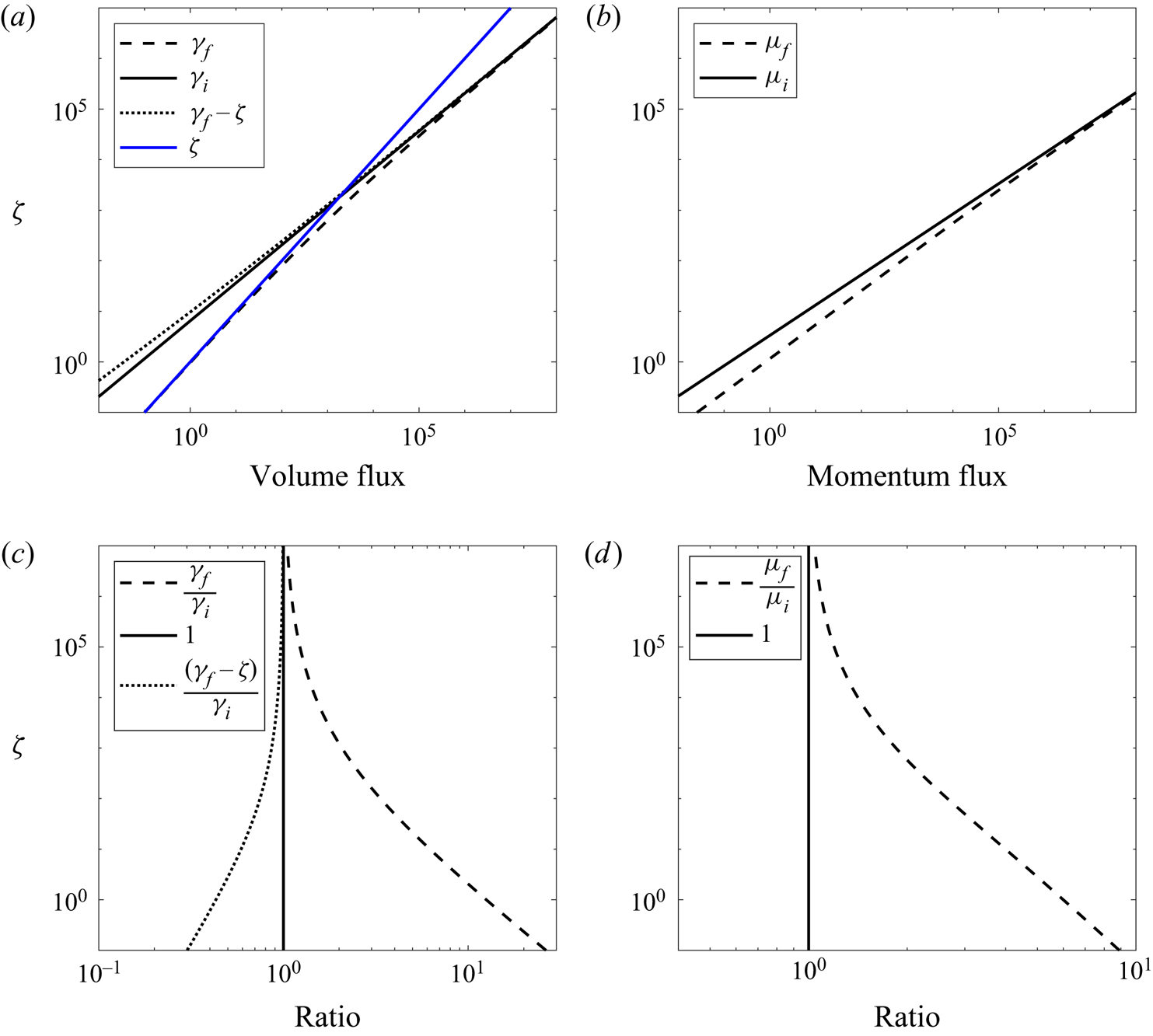
  $0.91\ \textrm {ml}\ \textrm {rev}^{-1}$. A diagram of the experimental set-up is shown in figure 2. As the plume reaches the base of the tank a gravity current forms. The porous wall structure (figure 2b) was suspended above the base of the tank by a height of 0.20 m so that the gravity current, and the accumulation of plume fluid, would not significantly disturb the unstratified measurement region. The stainless steel porous plates were manufactured by SINTERTECH® and had a stainless steel alloy grade of SS 316 L. Given the pore size of the porous plate, ${\sim }{1.0}\ \mathrm {\mu }\textrm {m}$, the source solution was first filtered using a filter size of ${0.1}\ \mathrm {\mu }\textrm {m}$ to minimise blockages within the porous plate. For source fluid of uniform buoyancy the variation in source buoyancy flux over the height of the porous plate is determined by the variation in source volume flux. Here we consider how the source buoyancy and bulk source volume flux affect the variation in source volume flux through the porous plate.
Experimental set-up used to create and measure a vertically distributed buoyancy source. The coordinate system is shown on the left and on the right (a) the large reservoir, (b) the source chamber and porous wall structure, (c) the two cameras and (d) the laser. The camera set-up shown was used to perform particle image velocimetry (PIV) over the whole height of the wall. However, for the simultaneous laser induced fluorescence and PIV measurements the two camera measuring windows coincided.
The flow through the porous plates can be characterised by Darcy's law that states that in a laminar flow the pressure drop between the porous media is linearly proportionally to the flow rate through the porous media. The Reynolds number for the flow through the porous plates may be estimated by  ${\textit {Re}}=qd_p/\phi _p\nu$, where $d_p$ and $\phi _p$ are the average pore-hole size and porosity of the plate and $q$ is the volume flux per unit area through the plate. The range of $q$ used in the experiments are given in table 1. These values suggest that ${\textit {Re}}\sim 10^{-3}$, so that Darcy's law is valid for flows considered here. Darcy's law may be expressed as follows
 \begin{equation} q=\frac{P_0 {\rm \Delta} p}{d\mu}, \end{equation}
where  ${\rm \Delta} p$ is the pressure difference either side of the porous plate and
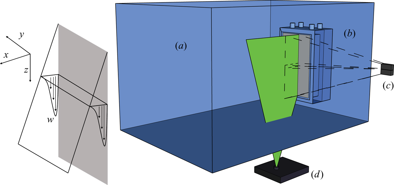
  $\mu$ is the dynamic viscosity of the source solution. An illustration of the following model is shown in figure 3.
Simplified diagram (not to scale) of the structure used to force relatively dense source fluid with a density of  $\rho _s$ through two porous plates of thickness $d$ at a bulk flow rate per unit width of $Q_s$.
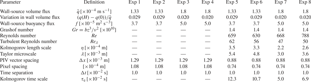
Experimental parameters and measured length and time scales of the experiments. Since the measurements were performed over the whole height in experiments 1–4 the characteristic scales are not included. For experiments 5–8 the characteristic scales are measured at  $z=0.37 \ \textrm {m}$, which is approximately the mid-height of the measurement window. Definitions are provided in the text.
The gear pump supplies fluid of density  $\rho _s$ and dynamic viscosity $\mu$ to the first chamber which results in pressure $p_1(z)$, where
 \begin{equation} p_1(z)=p_1(0)+\rho_sgz, \end{equation}
and  $p_1(0)$ is the pressure at the top of the chamber which is imposed via a gear pump. Similarly, the pressure in the second chamber is given by
 \begin{equation} p_2(z)=p_2(0)+\rho_sgz, \end{equation}
and the pressure in the ambient environment is given by
 \begin{equation} p_e(z)=p_e(0)+g \int_0^z \rho_e(z') \,\mathrm{d} z', \end{equation}
where we assume the ambient density  $\rho _e(z)$ is height dependent for the general case of a stratified experiment. Applying Darcy's law (3.1) to the first porous plate gives
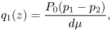 \begin{equation} q_1(z)=\frac{P_0(p_1-p_2)}{d \mu}, \end{equation}
where  $q_1(z)$ is the volume flux per unit area through the first porous plate. Similarly, for the second porous plate
 \begin{equation} q_2(z)=\frac{P_0(p_2-p_e)}{d \mu}, \end{equation}
where  $q_2(z)$ is the volume flux per unit area through the second porous plate. By neglecting vertical motion within the chambers, i.e. assuming that $q(z)=q_1(z)=q_2(z)$, and substituting in (3.2) and (3.3), we obtain
 \begin{equation} q(z)=\frac{P_0}{2\,d \mu}\left(p_0+g\rho_sz-g\int_0^z \rho_e(z')\,\textrm{d} z'\right), \end{equation}
where  $p_0=p_1(0)-p_e(0)$. The difference in the volume flux per unit area between the top and bottom of the porous plate, relative to the mean flow rate, is given by
 \begin{equation} \frac{q(H)-q(0)}{\bar{q}}=\frac{P_0g}{2\bar{q}\,d \mu}\left(\rho_sH-\int_0^H \rho_e(z)\,\textrm{d} z\right), \end{equation}
where  $\bar {q}=Q_s/H$. The maximum difference in flow rate may be evaluated by considering the case $\rho _e(z)=\rho _a$, i.e. where the ambient is unstratified. In practice a chosen bulk volume flux $Q_s$, as opposed to a chosen pressure, is imposed through the porous plate. The maximum difference in flow rate can therefore be written in terms of the initial density difference and the mean flow rate
 \begin{equation} \frac{q(H)-q(0)}{\bar{q}}=\frac{P_0gH\left(\rho_s-\rho_a\right)}{2 \bar{q}\,d \mu}. \end{equation}
These values are shown in table 1, which shows that there is at most a  $1.5\,\%$ variation in the source volume flux per unit area, relative to the mean source volume flux per unit area. We therefore make the approximation that the volume flux per unit area is uniform and equal to the mean volume flux per unit area which we refer to from hereon by $q$. The source fluid, with buoyancy $b_s$, then results in a mean buoyancy flux per unit area of $f = q b_s$. Cooper & Hunt (Reference Cooper and Hunt2010) used a similar experimental set-up to study vertically distributed buoyant plumes. However, as highlighted in their study, the relatively high porosity of their wall led to a non-uniform buoyancy flux. This problem is significantly reduced in the set-up used here.
Results given in § 2 may be used to determine how the added volume from the wall source modify the theoretical flow from the ideal solutions of zero volume flux. From table 1 the maximum vertical non-dimensional distance of the experiments may be calculated to give  $\zeta =8.4\times 10^6$ for experiments $1$,
$1$,  $2$,
$2$,  $5$ and $6$ and $\zeta =4.1\times 10^6$ for experiments $3$,
$3$,  $4$,
$4$,  $7$ and $8$. The results from figure 1 suggest that the volume and momentum flux of the finite-flux plume are within $10\,\%$ of the ideal plume solutions for the region $z>{0.25}\ \textrm {m}$ in our experiments. Among other restrictions, the theory assumes that the plume is fully turbulent and self-similar over the whole height, which is effectively modelled by a constant entrainment coefficient and constant $\theta$. This assumption is clearly not valid in the laminar region of the plume which accounts for approximately $15\,\%$ of the total height, consistent with the observation of Cooper & Hunt (Reference Cooper and Hunt2010). Further, as noted by Kaye & Cooper (Reference Kaye and Cooper2018), it is not possible to define a virtual origin elsewhere to the physical origin. Caudwell et al. (Reference Caudwell, Flór and Negretti2016) accounted for the laminar region in their numerical model (which was based on the work of Germeles Reference Germeles1975) by using laminar similarity solutions for the region below a critical height and plume theory for the turbulent region above this height. They determined the critical height based on the instantaneous Grashof number. In order to identify the laminar region in our experiments, determine the effect of the laminar region on the flow and, in particular, identify the region which follows the scalings predicted by Cooper & Hunt (Reference Cooper and Hunt2010), velocity measurements over the whole height of the porous wall were performed initially. Images from two cameras were recorded simultaneously, one for the region $z={0}\ \textrm {m}$ to $z={0.25}\ \textrm {m}$ and another for the region $z={0.23}\ \textrm {m}$ to $z={0.48}\ \textrm {m}$, so that there was a small overlapping region.
Measurements of the velocity fields on an  $x$–
$x$– $z$ plane were taken using particle image velocimetry. A frequency-doubled dual-cavity Litron Nano L100 Nd:YAG pulsed laser with wavelength $532\ \textrm {nm}$ was used to create a light sheet with a thickness of $1\text {--}2\ \textrm {mm}$ in the measurement section. The illuminated sheet was then imaged using two AVT Bonito CMC-4000 4 megapixel CMOS cameras, as shown in figure 2. Polyamide particles with mean diameter $2\times 10^{-2}\ \textrm {mm}$ and density $1.02\times 10^{3}\ \textrm {kg}\ \textrm {m}^{-3}$ were added to the ambient fluid. Images were simultaneously captured at 100 Hz before being processed. The PIV vector spacing gives a bound on the resolution of the boundary layer, suggesting that the boundary layer can not be accurately resolved for near-wall regions $x<{0.88}\ \textrm {mm}$. In order to minimise the effects of the reflection from the wall on the near-wall region, a background removal process was first implemented on the raw images before PIV processing. To determine the velocity fields, the raw particle images were processed using the 2017a PIV algorithm of Digiflow (Olsthoorn & Dalziel Reference Olsthoorn and Dalziel2017). Interrogation windows were chosen to be $24 \times 24\ \textrm {pixels}^2$ with an overlap of 50 %, which resulted in a velocity vector every 1.29 mm. After the images were processed, the velocity fields from each region were mapped to a common world coordinate system using a calibration target of regular dots aligned with the laser sheet resulting in a velocity field over the whole height of the wall.
Given the results of the velocity measurements over the total height, a further set of simultaneous velocity and buoyancy field measurements were performed within the region  $z={0.30}\ \textrm {m}$ to $z=0.42\ \textrm {m}$, which was sufficiently far from the source so that the plumes can be considered turbulent and self-similar, and is discussed further in § 4.1. Further, the flow is shown to be consistent with both the ideal plume solutions (2.14)–(2.16) and previous experimental and numerical investigations of turbulent vertically distributed buoyancy sources, including those with zero added source mass flux.
Simultaneous measurements of the velocity and density fields on an  $x$–
$x$– $z$ plane were taken using PIV and LIF. An identical laser configuration was used as described above. The illuminated sheet was then imaged using two AVT Bonito CMC-4000 4 megapixel CMOS cameras, one for the PIV and one for the LIF. The PIV was performed as described above for the velocity measurements, resulting in a velocity vector every 0.88 mm. To allow LIF measurements, a low concentration of the fluorescent dye Rhodamine 6G ( $9.1\times 10^{-6}\ \textrm {kg}\ \textrm {m}^{-3}$ for all the experiments) was added to the source fluid. To separate the two signals, i.e. separate the light scattered from the particles from that fluoresced by the dye, a narrow bandpass filter (centred at the wavelength of the laser) was placed in front of the PIV camera and a longpass filter was placed in front of the LIF camera. Images for both PIV and LIF were simultaneously captured at 100 Hz before being processed.
For the density field, given the low concentrations of Rhodamine 6G in the source solution and dilution through entrainment into the plume, a linear relationship between the light intensity perceived by the camera and the dye concentration was used to determine the density field as in Ferrier, Funk & Roberts (Reference Ferrier, Funk and Roberts1993). For the experiments described in this paper, a two-point calibration was performed by capturing an image of the background light intensity and an image at a known dye concentration, where in each case the ambient sodium chloride solution was identical to that used in the experiments. Both calibration images were captured with the polyamide particles within the tank, at the seeding density used for the experiment, to account for differences in the laser intensity due to the presence of the particles. Parker et al. (Reference Parker, Burridge, Partridge and Linden2020) used the same laser, ambient tank and camera to perform LIF on a wall and free plume. They performed a detailed analysis of the effect of the attenuation of the laser on the LIF measurements by measuring the extinction coefficient of the Rhodamine 6G and added salts and calculating the effective dye concentration that the laser beam rays pass through. Using an identical methodology we estimate that the error in the LIF measurements, as a result of the laser attenuation, is at most  $2\,\%$. The spatial resolution of the processed LIF images was 0.074 mm.
After the images were processed, the velocity and density fields were mapped to a common world coordinate system. This was accomplished for both cameras by imaging a calibration target of regular dots aligned with the laser sheet. As an additional calibration step, a sequence of particle images were captured on both cameras, with their filters removed, simultaneously. Similar to stereo PIV calibration, e.g. Willert (Reference Willert1997), these particle images were then cross-correlated to determine a disparity map and shift the coordinate mappings to compensate for any small misalignment between the calibration target and the light sheet, an identical procedure to that described in Parker et al. (Reference Parker, Burridge, Partridge and Linden2020).
Measurements were collected over a measurement window height of 0.12 m starting at a distance 0.30 m from the top of the porous plate. These regions were sufficiently far from the source so that the flow can be considered turbulent and self-similar. Each experiment was recorded for 100 s, corresponding to  $10^4$ simultaneous velocity/density fields. A total of eight plumes were studied, four examining the velocity field over the whole height of the wall and four examining the velocity and buoyancy field over a region considered to be turbulent and self-similar. The effect of the finite duration time-averaging window on our results is discussed in appendix A.
The experimental source parameters are given in table 1. Also given for the simultaneous experiments are the Grashof number  $Gr=bz^3/\nu ^2$, Reynolds number ${\textit {Re}}=\bar {w}_mR/\nu$, the turbulent Reynolds number ${\textit {Re}}_{\lambda }=\overline {w'}_{rms}\lambda /\nu$, the Kolmogorov length scale $\eta =(\nu ^3/\epsilon )^{1/4}$, the Taylor microscale $\lambda =\overline {w'}_{rms}\sqrt {15\nu /\epsilon }$ and the Kolmogorov time scale $\tau _{\eta }=(\nu /\epsilon )^{1/2}$, where $\epsilon =15\nu \overline {(\partial w/\partial z)^2}$ and $Sc$ is the Schmidt number, all evaluated at the mid height of the region examined. The subscript $rms$ denotes the root mean square of the data.
4. Results
4.1. Velocity measurements over the whole domain
Figure 4 shows an instantaneous buoyancy field taken from experiment  $5$. The image shows the typical width, approximately 20 mm, of the distributed wall-source plume in the experiments. In order to increase precision of the velocity measurements it was necessary to focus on a smaller region. In order to identify the optimal region to focus on, namely where the plume has become fully turbulent, self-similar and obtained an invariant balance between momentum and buoyancy (i.e. become pure), we first present results of the experiments examining the whole height of the distributed wall-source plume.
An instantaneous buoyancy field of the distributed wall-source plume resulting from the vertically distributed buoyancy source taken from experiment  $5$. The figure is rotated through $90^\circ$ for clarity.

The height at which the flow transitions to turbulence may be determined by examining the Reynolds stress. Figures
5(a)–5(d) show the Reynolds stress for the four experiments 1–4 and figure 5(e) shows the maximum Reynolds stress as a function of height for the region  $z<{0.16}\ \textrm {m}$. The data suggest that the transition to turbulence occurs at approximately 0.08 m. Figure 6(a) shows the Richardson number, defined by $Ri=f z Q_p^3/M^3$, as a function of the distance from the base of the source $z={0}\ \textrm {m}$ for these four experiments. The Richardson number decreases from a relatively large value and tends to a constant value of $Ri\approx 0.20$. A high Richardson number is expected in the laminar region given that the buoyancy flux is being forced through the plate at very low momentum, i.e. there will be an excess buoyancy relative to the momentum. As the flow transitions to turbulence the Richardson number decreases. The Richardson number reaches a statistically steady value at $z\approx {0.25}\ \textrm {m}$ suggesting that the plume is pure for $z>{0.25}\ \textrm {m}$.
(a–d) Time-averaged Reynolds stress for experiments 1–4, respectively, and (e) the maximum time-averaged Reynolds stress, plotted against the height, highlighting the transition to turbulence in the flow. Note that in (a–d) the horizontal coordinate is scaled, relative to the vertical coordinate, in order to aid clarity.

(a) Richardson number, (b) volume flux, (c) compensated plot of the volume flux and (d) the gradient of the logarithm of the volume flux of the vertically distributed buoyant plume for experiments 1–4. The scaling  $Q\sim z^{4/3}$, predicted by Cooper & Hunt (Reference Cooper and Hunt2010), is exhibited by the data in (c). The grey highlighted region in all four plots indicate the region where the Richardson number has reached a statistically steady state and where the volume flux follows the predicted scaling. This region is defined by where the mean gradient of the logarithm of the volume flux (black curve) is within one height-averaged standard deviation, $\tilde {\sigma }$, of $\mathrm {d}(\log {Q_e/f^{1/3}})/\mathrm {d} z=4/3$, where $\sigma (z)$ is the standard deviation of all four experiments measured at a given height. This region was identified in order to examine the plume at higher resolution with simultaneous velocity and buoyancy measurements. The average volume flux across the experiments is shown by the black curve in (b). The mean value of the Richardson number within this region of $Ri=0.20$ is shown by the horizontal dashed line in (a).
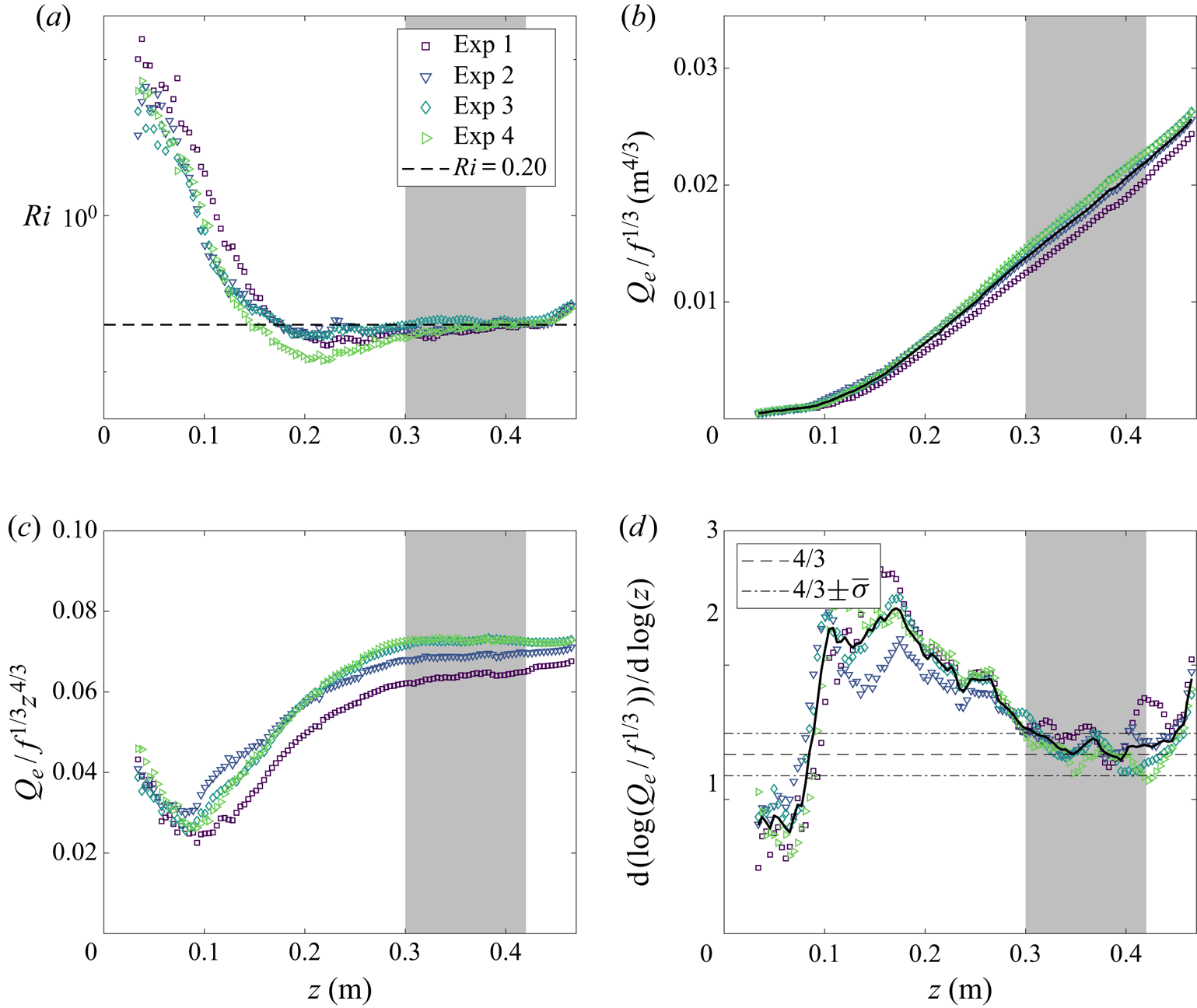
Figure 6(b) shows the volume flux of the four experiments. As discussed in § 2, the cumulative entrained flux, that is  $Q_e=Q-qz$, provides a more robust analogy to the ideal plume volume flux. For this reason, we present and compare $Q_e$ to the theoretically derived results of an ideal source. Unless otherwise stated, we refer to the cumulative entrained flux as the volume flux, however, to avoid confusion we maintain the notation $Q_e$. The compensated plot of the volume flux, where the volume flux is scaled on the predicted $z^{4/3}$, is shown in figure 6(c). Figure 6(d) shows the gradient of the logarithm of the volume flux. The standard deviation $\sigma (z)$ across all four experiments was calculated and the height-averaged value is defined by $\tilde {\sigma }$. The horizontal dashed and dot-dashed lines show the predicted scaling value of $4/3$ and $4/3\pm \tilde {\sigma }$, respectively. Higher-resolution simultaneous buoyancy and velocity measurements were performed within the region for which the mean value of the data lies within the range $4/3\pm \tilde {\sigma }$. This region is highlighted in grey in all four plots. The porous wall was suspended above the base of the ambient tank. The effect of this on the flow can be seen in the region $z> {0.44}\ \textrm {m}$ in figure 6(c), where the scaling deviates from the predicted value. We therefore choose to perform further higher-resolution simultaneous velocity and buoyancy measurements within the region ${0.30}\ \textrm {m} < z < {0.42}\ {\rm m}$. The next section presents the results from within this region.
4.2. Simultaneous velocity and buoyancy measurements
In this section we present the high-resolution simultaneous velocity and buoyancy measurements of the vertically distributed wall-source plume within the developed region.
Figure 7 shows the scaled vertical and horizontal velocities and buoyancy profiles for five heights spanning the measurement window from experiments 5–8. A good collapse of the data on to a single curve is seen in each plot. The vertical velocity data are compared to the profile of best fit to the previous data of Vliet & Liu (Reference Vliet and Liu1969), shown by the dashed red curve. Note that Vliet & Liu (Reference Vliet and Liu1969) non-dimensionalise the cross stream distance by the displacement thickness defined by  $\delta _h=\int _0^{\infty }\bar {w}/\bar {w}_{m} \,\mathrm {d} x$. We have rescaled their data by identifying a linear relationship between the displacement thickness and vertical distance shown in figure 7(d). Our vertical velocity data show good agreement with that of Vliet & Liu (Reference Vliet and Liu1969). Note that only the function of the average temperature data is presented in Vliet & Liu (Reference Vliet and Liu1969), therefore the corresponding buoyancy profile will vary according to the experimental parameters, so it is not compared to our buoyancy data.
Time-averaged scaled (a) vertical and (b) horizontal velocity and (c) buoyancy profiles of the vertically distributed turbulent plume for heights  $z=0.302$, $0.331$, $0.360$, $0.389$ and 0.418 m from experiments 5–8. The profile of best fit from the velocity data of Vliet & Liu (Reference Vliet and Liu1969), which agree well with the data of Cheesewright (Reference Cheesewright1968), is shown by the dashed red curve. Vliet & Liu (Reference Vliet and Liu1969) scaled the horizontal distance by the displacement thickness defined by $\delta _h=\int _0^{\infty }\bar {w}/\bar {w}_{m} \,\mathrm {d} x$. (d) A least-squares linear fit between the displacement thickness and the vertical distance was found in order to rescale the data of Vliet & Liu (Reference Vliet and Liu1969) by the vertical distance.
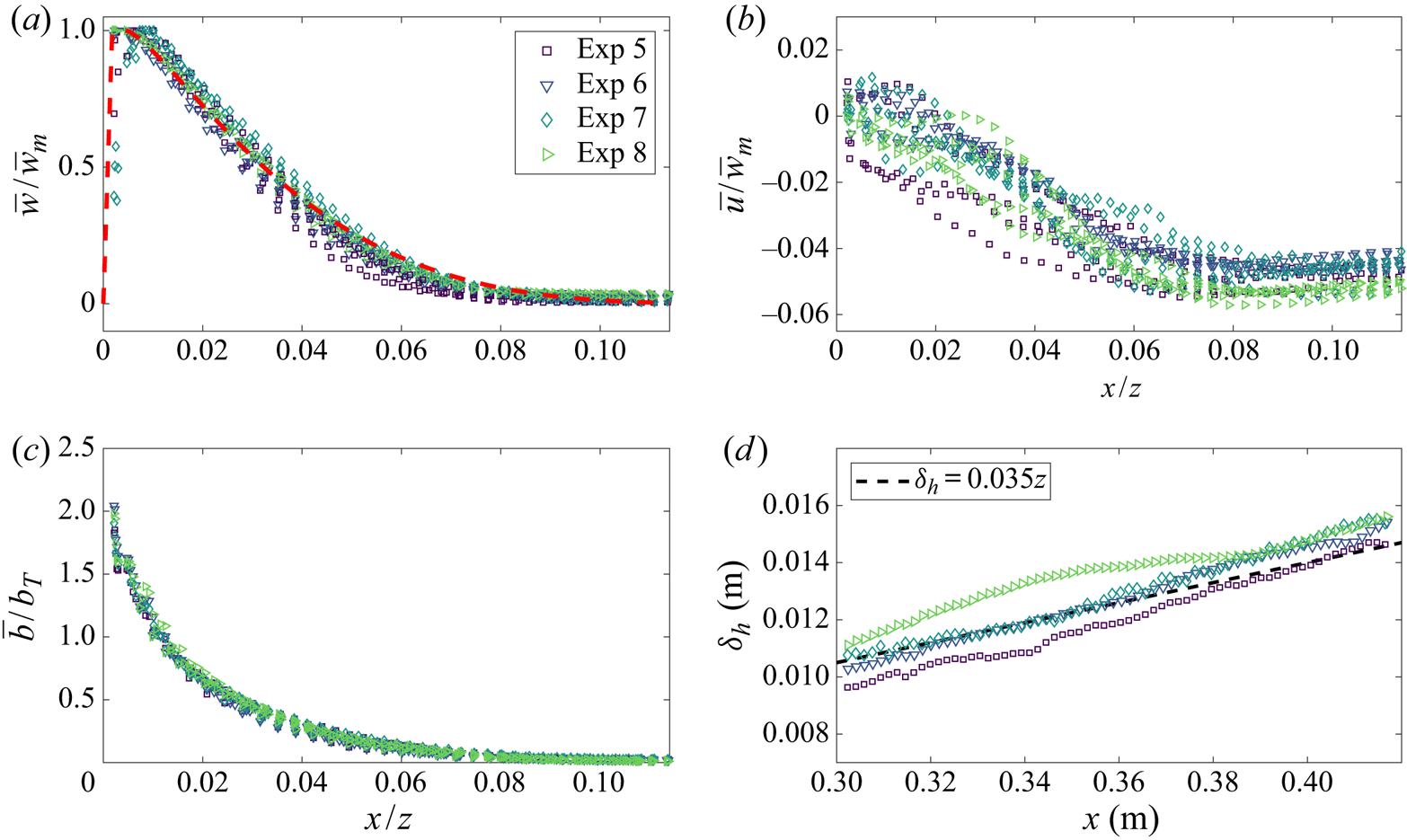
The maximum time-averaged vertical velocity, scaled on the characteristic vertical velocity, is shown in figure 8(a) highlighting a linear relationship between the two velocity scales. The volume and momentum fluxes for experiments 5–8 are also shown in figure 8 where the fluxes are compensated by their predicted scalings. The averages of the data over height and across the four experiments are shown by the dashed line in each case. Good agreement between the data and the predicted scalings of (2.20)–(2.22) are observed in all cases. Also shown in figure 8(d) are the data for the compensated integral buoyancy  $B$. Equation (2.15) suggests that $B=c_Bf^{2/3}z^{2/3}$ for some constant prefactor $c_B$. Gayen et al. (Reference Gayen, Griffiths and Kerr2016) also observe the scalings found above for the volume and momentum fluxes, however, they identify modified scaling prefactors to those predicted by Cooper & Hunt (Reference Cooper and Hunt2010). Instead, Gayen et al. (Reference Gayen, Griffiths and Kerr2016) observed that $Q=c_Qf^{1/3}z^{4/3}$ and $M=c_Mf^{2/3}z^{5/3}$, where $c_Q=0.076$ and $c_M=0.13$. Our results in figure 8 show reasonable agreement with Gayen et al. (Reference Gayen, Griffiths and Kerr2016), with $c_Q=0.070\pm 0.006$ and $c_M=0.11\pm 0.02$. In addition we find that $c_B=0.53\pm 0.06$.
(a) The maximum time-averaged vertical velocity scaled on the characteristic vertical velocity and compensated plots of time-averaged (b) volume flux, (c) momentum flux and (d) integral buoyancy as functions of height for experiments 5–8. The height-averaged data, which are also averaged across the four experiments, are shown in each case by the dashed line, with the value shown in the legend.
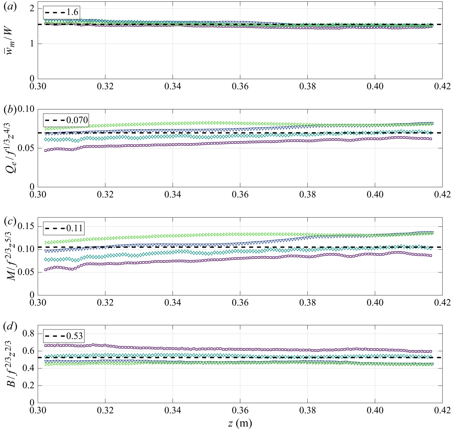
In the region under examination, the entrainment velocity  $\mathrm {d} Q_e/\mathrm {d} z$ is much larger than the source volume flux $q$. In particular, $q/(\mathrm {d} Q_e/\mathrm {d} z)<0.07$ for $z>{0.30}\ \textrm {m}$ for all the experiments. The mean skin friction coefficient, based on the characteristic vertical velocity, may be estimated using (2.15) and the results from figure 8 to determine that $C\approx 0.15$. This value is slightly lower than the value $C\approx 0.18$ obtained by Gayen et al. (Reference Gayen, Griffiths and Kerr2016). However, as they note, the values are likely to differ in experiments where there is a wall-source volume flux, such as Cooper & Hunt (Reference Cooper and Hunt2010) and the present experimental set-up, as compared to buoyancy primarily diffusing from the boundary, such as that of McConnochie & Kerr (Reference McConnochie and Kerr2015) and Gayen et al. (Reference Gayen, Griffiths and Kerr2016).
The entrainment coefficient may be estimated by using the relation  $3\alpha /4 =\mathrm {d} R/\mathrm {d} z$, which may be derived from the solutions (2.20)–(2.21). Using the results from figure 8 gives
 \begin{equation} \alpha =\frac{4}{3}\frac{\mathrm{d} }{\mathrm{d} z}\left(\frac{Q_e^2}{M}\right)=0.062\pm 0.009. \end{equation}
The entrainment coefficient should, however, be thought of as the ratio of the entrainment velocity to the characteristic vertical velocity. In which case, the corrected volume flux, i.e.  $Q_e$, should not be used in the calculation of the mean velocity. The entrainment coefficient can be calculated more robustly by considering
 \begin{equation} \alpha=\frac{Q_p}{M}\frac{\mathrm{d} Q_e}{\mathrm{d} z}=-\frac{Q_p}{M}\bar{u}_{\infty}=0.068\pm0.006. \end{equation}
The velocity  $\bar {u}_{\infty }$ as a function of height for experiments 5–8 is plotted in figure 9. As expected, the value of $\alpha$ calculated from (4.2) is larger than that of (4.1) due to the corrected volume flux; however, the two values agree reasonably well. Our calculated entrainment coefficient falls within the wide range of previously reported values, which were calculated using velocity measurements, of $\alpha =0.059$ by Gayen et al. (Reference Gayen, Griffiths and Kerr2016), $\alpha =0.048\pm 0.006$ by McConnochie & Kerr (Reference McConnochie and Kerr2015) and $\alpha =0.08$ by Caudwell et al. (Reference Caudwell, Flór and Negretti2016).
Entrainment coefficient measured directly from the far field horizontal velocities,  $\bar {u}_{\infty }$, and the mean top-hat velocity, W. The mean far field horizontal velocity, for a given height, was calculated by averaging, in the horizontal direction, the horizontal velocities between $x_1= {0.036}\ \textrm {m}$ and $x_2={0.048}\ \textrm {m}$, so that $\bar {u}_{\infty }(z)=\int _{x_1}^{x_2}\bar {u}{(x,z)} \,\mathrm {d} x$.
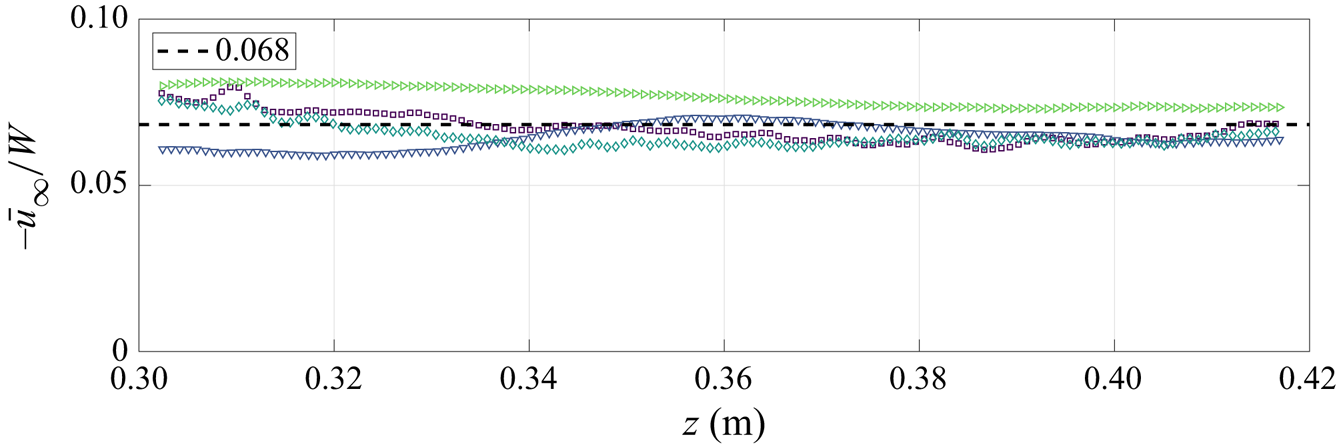
The ideal plume solutions (2.20)–(2.22) implicitly assume that the similarity coefficient  $\theta$, that encapsulates the relation between the integral buoyancy $B$ and the buoyancy flux $F$, takes a constant value of $\theta \approx 1$. Figure 10 shows the value of $\theta$ for the full height of the measurement window for all four experiments. An average value, across all the experiments, of $\theta =0.84$ was found. We may, therefore, assume that any analysis involving the volume flux solution is not significantly affected by ignoring the $\theta$ term in (2.20), since the solution is modified by a factor of only $\theta ^{1/3}=0.94$.
Measurements of the similarity coefficient  $\theta =BM/FQ_p$ from the four experiments 5–8. The average value across all heights and experiments $\theta =0.84$ is shown by the dashed line.
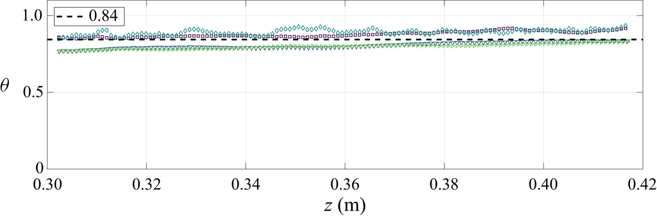
On average, the compensated volume and momentum fluxes are larger in experiments  $7$ and $8$ (i.e. the experiments with larger source volume and buoyancy fluxes) and, similarly, smaller in the compensated buoyancy integral. While the larger source volume flux may have an effect on the average discrepancy, the variation is not significant compared to the experimental uncertainty. Indeed, the compensated buoyancy integral, and $\theta$, of experiments $6$ and $8$ closely align. In addition, there appears to be no systematic dependency on the source conditions on the average entrainment velocity.
4.3. Turbulent fluctuations
Figure 11 presents the normalised root mean square (rms) velocity and buoyancy profiles, Reynolds stress and the horizontal and vertical buoyancy fluxes for five heights spanning the measurement window from experiments 4–8. To our knowledge, the only existing data to compare with are the rms of the vertical velocities of Vliet & Liu (Reference Vliet and Liu1969). Although their data are relatively scattered, a peak value of approximately  $0.25$ is observed, in good agreement with a peak value of about $0.27$ observed in our measurements. The data show that the fluctuations in vertical velocity are of the same order of magnitude as the fluctuations in the horizontal velocity, cf. the mean vertical and horizontal velocities which differ by nearly two orders of magnitude. Note, however, that the turbulent vertical transport of buoyancy is an order of magnitude larger than the turbulent horizontal transport of buoyancy as a result of the expected strong correlation between buoyant parcels of fluid and upward motion.
Time-averaged scaled turbulent fluctuations of (a) vertical velocity, (b) horizontal velocity and (c) buoyancy, (d) Reynolds stress and (e) vertical and (f) horizontal turbulent buoyancy flux for heights  $z=0.302$, $0.331$, $0.360$, $0.389$ and 0.418 m from experiments 5–8.
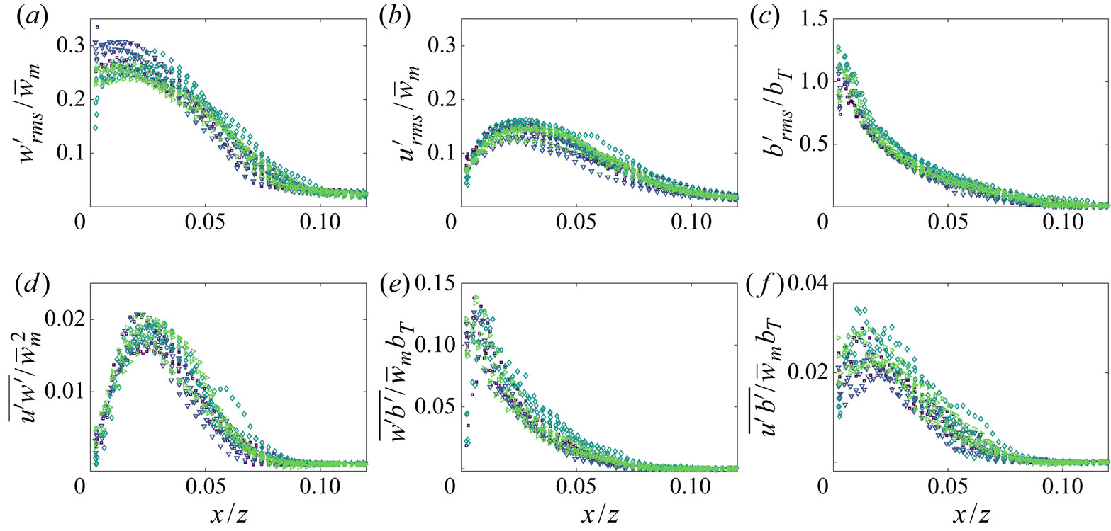
The turbulent viscosity and turbulent diffusivity were also calculated and are shown in figure 12(a). Experimental observations of these quantities rely on both second-order quantities and the gradients of first-order quantities. In particular, both the turbulent transport quantities and the gradients of the vertical velocity and buoyancy approach zero at infinity, in addition to the zero velocity gradient at the maximum vertical velocity. Large errors in the calculation of the turbulent viscosity and turbulent diffusivity from experimental data may therefore by expected away from the regions with large shear. In an attempt to overcome this we first calculate the mean profiles, across all four experiments, of the time-averaged self-similar profiles shown in figure 11. The calculations were then performed on these mean profiles. We show only data within the turbulent core of the plume, away from both the maximum vertical velocity and the ambient region of the plume.
(a) The mean time-averaged turbulent viscosity,  $\nu _T=-\overline {u'w'}/(\mathrm {d} \bar {w}/{\mathrm {d} z})$, and turbulent diffusivity, $\kappa _T=-\overline {u'b'}/ (\mathrm {d} \bar {b}/{\mathrm {d} z})$, from experiments 5–8. Data are only shown for regions where small gradients of the mean flow quantities do not result in unreliable measurements. (b) The turbulent Schmidt number, $Sc_T=\nu _T/\kappa _T$.
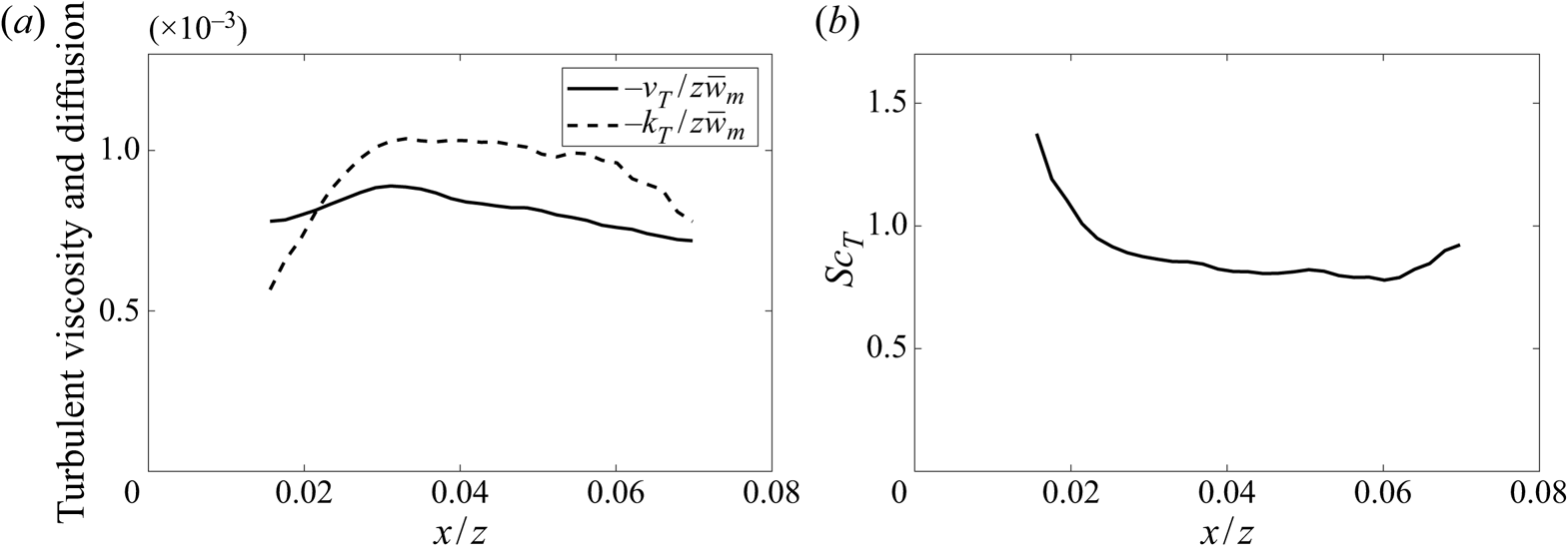
While the turbulent viscosity is approximately constant across the core of the plume, the turbulent diffusivities decreases rapidly for  $x/z<0.25$. This may be a result of the large buoyancy gradients observed within this region and may contribute more significantly to the error than for the turbulent viscosity.
The turbulent Schmidt number, shown in figure 12(b), was calculated using the profiles shown in shown in figure 12(a) and gives a mean value of  $Sc_T=0.9$ across the region for which the data are shown. This value is in line with previously reported Schmidt and Prandtl numbers in wall-bounded buoyant flows (Kader & Yaglom Reference Kader and Yaglom1972; Lai & Faeth Reference Lai and Faeth1987).
4.4. Comparison with wall line plume
Here we compare the vertically distributed buoyant plume to its equivalent-geometry conserved buoyancy flux counterparts, that is the free plume, the flow resulting from a horizontal line source of buoyancy absent of any boundaries, and a wall (line) plume, the flow resulting from a horizontal line source of buoyancy immediately adjacent to a wall, both of which were studied by Parker et al. (Reference Parker, Burridge, Partridge and Linden2020). As highlighted by Kaye & Cooper (Reference Kaye and Cooper2018), ‘plumes generated by vertically distributed sources of buoyancy have been observed to have substantially lower entrainment coefficients than their equivalent-geometry constant buoyancy flux plumes’. Kaye & Cooper (Reference Kaye and Cooper2018), however, primarily refer to the free plume as the equivalent-geometry plume to the distributed wall-source plume and discuss reasons for the reduced entrainment between these two flows, including the shear stress and the suppression of eddy meandering.
Our findings support their observation that the distributed wall-source plume has a significantly lower entrainment coefficient,  $\alpha =0.068\pm 0.006$, than the free plume, $\alpha _f=0.135\pm 0.010$, however, we find only a small reduction compared to the wall plume, $\alpha _w=0.076\pm 0.006$ (Parker et al. Reference Parker, Burridge, Partridge and Linden2020). The relative difference between $\alpha$ and $\alpha _w$ is noticeably smaller than previous findings, where $\alpha$ ranges from $0.014$ to $0.08$ (Cooper & Hunt Reference Cooper and Hunt2010; McConnochie & Kerr Reference McConnochie and Kerr2015; Caudwell et al. Reference Caudwell, Flór and Negretti2016; Gayen et al. Reference Gayen, Griffiths and Kerr2016; Bonnebaigt et al. Reference Bonnebaigt, Caulfield and Linden2018) and $\alpha _w=0.1$ (Bonnebaigt et al. Reference Bonnebaigt, Caulfield and Linden2018), which merited such an in depth discussion by Kaye & Cooper (Reference Kaye and Cooper2018). By studying two flows that differ only by the presence of a wall, Parker et al. (Reference Parker, Burridge, Partridge and Linden2020) concluded that the wall significantly reduces entrainment in a wall plume, as compared to a free plume. The large difference in the entrainment coefficients between the distributed wall-source plume and the free plume, and the small difference between the distributed wall-source plume and the wall plume, suggests that the reduction in the entrainment coefficient in the vertically distributed wall-source plume is primarily a result of the presence of the wall, rather than a consequence of the vertically distributed buoyancy flux.
However, the slightly lower value, compared to the wall plume, suggests that vertically distributed buoyancy also makes a minor contribution to reducing entrainment. Based on the conclusions of Parker et al. (Reference Parker, Burridge, Partridge and Linden2020), it is reasonable to conclude here that the significant reduction in entrainment observed in the distributed wall-source plume relative to free-shear buoyancy-driven flows (also compare to  $\alpha _{p}\approx 0.11$ in an axisymmetric plume, Burridge et al. Reference Burridge, Parker, Kruger, Partridge and Linden2017) is primarily a result of the suppression of large-scale coherent structures (which have been shown to dominate the flow, e.g. Burridge, Partridge & Linden Reference Burridge, Partridge and Linden2016), and the wall inhibiting meandering of the plume both leading to reduced turbulent mixing by the plume.
Figure 13 compares the velocity, buoyancy and the Reynolds stress of the distributed wall-source plume and the wall line plume. The wall line plume data have been scaled using the source buoyancy flux. Further, the vertical distance includes a virtual origin correction as described in Parker et al. (Reference Parker, Burridge, Partridge and Linden2020). Figure 13(a) shows larger peak velocities in the wall plume, for a given buoyancy flux. However, figure 13(b) shows significantly larger peak buoyancy in the distributed wall-source plume. This is opposite to the observation of larger peak velocities and buoyancy in the wall plume, relative to the free plume (Parker et al. Reference Parker, Burridge, Partridge and Linden2020, figure 17b), which suggested that the larger velocities were a result of larger mean buoyancy magnitudes. This implies that the buoyancy is less able to be effectively mixed in the distributed wall plume, as the lower peak Reynolds stress values in figure (c) suggest, so that the constrained buoyancy leads to a peak velocity very close to the wall, as can be seen figure 13(a), thereby leading to a large shear stress. A peak velocity very close to the wall has also been observed in Gayen et al. (Reference Gayen, Griffiths and Kerr2016) which they argue leads to large momentum drag. This is reflected in the value of the skin friction coefficient found of  $C=0.15$, equivalent to $65\,\%$ of the buoyancy force (also observed by Gayen et al. Reference Gayen, Griffiths and Kerr2016), compared to $C=0.015$ in the wall plume observed by Parker et al. (Reference Parker, Burridge, Partridge and Linden2020), which is equivalent to $15\,\%$ of the buoyancy force.
Comparison of the average profiles of the time-averaged (a) vertical velocity, (b) buoyancy and (c) Reynolds stress from the distributed wall-source plume (black) and the wall line plume (blue) using data from Parker et al. (Reference Parker, Burridge, Partridge and Linden2020). In the case of the wall line plume, the vertical distance has been corrected using a virtual origin and the source buoyancy flux.
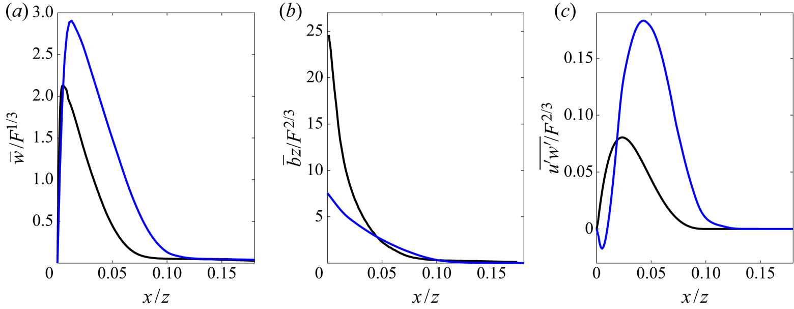
The effects on bulk entrainment are twofold; firstly the presence of a rigid boundary results in a lower entrainment coefficient (compared with free line plumes), and secondly the vertically distributed nature of the buoyancy forcing results in lower characteristic vertical velocities (compared with wall line plumes). These two effects combine to significantly reduce the volume flux entrained by vertically distributed wall-source plumes,  $Q=0.069F^{1/3}z$, compared to both free line plumes, $Q_f=0.40F^{1/3}z$, and wall line plumes, $Q_w=0.17F^{1/3}z$. This can be visualised from figure 13(a), where both a reduction in maximum velocity and plume width, characterised by the larger velocities away from the wall, can be seen.
5. Conclusions
The flow resulting from a vertically distributed wall source of buoyancy was studied by forcing dense source solution through a porous wall. By extending the numerical model of Kaye & Cooper (Reference Kaye and Cooper2018), the plume equations were solved to account for both a finite source volume flux and skin friction coefficient. The plume equations, however, do not account for the laminar region and a virtual origin correction is not possible. In order to identify the laminar region, determine the effect of the laminar region on the flow, and identify the region in which the flow is a turbulent self-similar pure-plume, two-dimensional plane velocity measurements normal to the wall were first performed over the whole height of the porous wall. For the experimental parameters used in this study the transition to turbulence was observed to occur at a height of approximately 0.08 m, although a pure-plume state was not reached until approximately 0.25 m, where the pure-plume criterion was based on an invariant Richardson number.
High-resolution simultaneous two-dimensional velocity and buoyancy measurements in a vertical plane normal to the wall were performed in a region found to exhibit the behaviour of a turbulent self-similar pure plume,  ${0.30}\ \textrm {m} < z < {0.42}\ \textrm {m}$. An entrainment coefficient of $\alpha =0.068\pm 0.006$ and a skin friction coefficient of $C=0.15$ were determined. The entrainment coefficient is not significantly smaller than the entrainment coefficient found for the wall line plume of $\alpha _w=0.076\pm 0.006$ (Parker et al. Reference Parker, Burridge, Partridge and Linden2020), suggesting that the reduction in entrainment compared to free line plume, $\alpha _f=0.135\pm 0.010$, is primarily due to the presence of the wall rather than the effect of the vertically distributed source of buoyancy. However, the slightly lower entrainment coefficient, compared to the wall line plume, suggests that the distributed nature of the buoyancy may reduce entrainment further.
Velocity, buoyancy and Reynolds stress profiles, scaled by the buoyancy flux and vertical distance, of the distributed wall-source plume were compared to those of the wall line plume using data from Parker et al. (Reference Parker, Burridge, Partridge and Linden2020). Lower peak velocities, and significantly larger peak buoyancies, were observed in the distributed wall-source plume. The position of the peak velocities are comparatively closer to the wall in the distributed wall-source plume, which supports the observation of a significantly larger skin friction coefficient. The large shear stress explains why larger peak velocities are not observed in the distributed wall-source plume, as would typically be expected given significantly larger buoyancy forcing. Significantly lower peak Reynolds stress profiles were also observed in the distributed wall-source plume, suggesting that the buoyant fluid is constrained near the wall and unable to be effectively mixed. This results in a larger buoyancy gradient, and therefore velocity gradient (i.e. shear stress) near the wall.
The reduced entrainment coefficient, compared with free line plumes as a result of the wall, and lower characteristic vertical velocities, compared with wall line plumes as a result of the vertically distributed nature of the buoyancy forcing, results in significantly reduced volume flux entrained by vertically distributed wall-source plumes.
Acknowledgements
We are grateful to the skilled technical staff of the G. K. Batchelor Laboratory for the manufacture of the apparatus and the illumination system. We also wish to acknowledge the contribution of Professor S. Dalziel to the data capture and processing. The work has received financial support from the UK Engineering and Physical Sciences Research Council through an iCASE award with Arup, the First Grant EP/R008957/1 ‘Confinement, boundaries and buoyancy in the mixing by fluid flows’ and also through the Programme Grant EP/K034529/1 ‘Mathematical Underpinnings of Stratified Turbulence’ (MUST), and from the European Research Council through the Horizon 2020 research and innovation programme agreement no. 742480 ‘Stratified turbulence and mixing processes’ (STAMP). The data associated with this paper can be found in the repository https://doi.org/10.17863/CAM.55351.
Declaration of interests
The authors report no conflict of interest.
Appendix A. Error associated with the finite duration time-averaging window
In order to assess the impact of the finite time-averaging window on our results we consider, for each experiment, the mean bulk flow quantities resulting from both the first and second half of the window. The time-averaged bulk flow quantities for  ${0}\ \textrm {s}\leq t <{50}\ \textrm {s}$ are defined as $Q_{1}$, $M_{1}$ and $B_{1}$ and for ${50}\ \textrm {s}\leq t \leq {100}\ \textrm {s}$ as $Q_{2}$, $M_{2}$ and $B_{2}$.
We define the mean variation,  $\mu _Q$, and error, $\sigma _Q$, in the volume flux as
 \begin{equation} \mu_Q=\frac{1}{z_2-z_1}\int_{z_1}^{z_2}\frac{Q_1-Q_2}{Q} \,\mathrm{d} z,\quad \sigma_Q=\left(\frac{1}{z_2-z_1}\int_{z_1}^{z_2}\left|\frac{Q_1-Q_2}{Q}\right|^2 \,\mathrm{d} z\right)^{1/2}, \end{equation}
where  $z_1$ and $z_2$ denote the measurement window and similarly for the momentum flux and buoyancy integral. The average, across the experiments, mean variations and errors associated with each quantity are given in table 2. The mean variations show that slightly higher volume flux and momentum flux values are obtained, on average, in the first half of the experiments and vice versa for the buoyancy integral. The errors associated with the bulk flow quantities are small compared to those of the standard deviation between experiments of ${\sim }10\,\%$ (cf. § 4), so that we conclude the finite duration of the experiments does not significantly affect our results.
The average, across all four experiments, of the mean variation and error as defined by (A 1) for the volume flux, momentum flux and buoyancy integral.
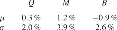


 Open access