
1. Introduction
Continuous Mortality Investigation (2016b) introduced a new model for fitting to mortality data: the Age-Period-Cohort-Improvement (APCI) model. This is an extension of the Age–Period–Cohort (APC) model, but it also shares an important feature with the model from Lee and Carter (Reference Lee and Carter1992). The APCI model was intended to be used as a means of parameterising a deterministic targeting model for mortality forecasting. However, it is not the purpose of this paper to discuss the Continuous Mortality Investigation’s approach to deterministic targeting. Readers interested in a discussion of stochastic versus deterministic projections, in particular the use of targeting and expert judgement, should consult Booth and Tickle (Reference Booth and Tickle2008). Rather, the purpose of this paper is to present a stochastic implementation of the APCI model for mortality projections, and to compare the performance of this model with various other models sharing similar structural features.
2. Data
The data used for this paper are the number of deaths d
x,y
aged x last birthday during each calendar year y, split by gender. Corresponding mid-year population estimates,
 $$E_{{x,y}}^{c} $$
, are also given. The data therefore lend themselves to modelling the force of mortality,
$$E_{{x,y}}^{c} $$
, are also given. The data therefore lend themselves to modelling the force of mortality,
 $$\mu _{{x{\plus}{1 \over 2},y{\plus}{1 \over 2}}} $$
, without further adjustment. However, for brevity we will drop the
$$\mu _{{x{\plus}{1 \over 2},y{\plus}{1 \over 2}}} $$
, without further adjustment. However, for brevity we will drop the
 $${1 \over 2}$$
and just refer to μ
x,y
.
$${1 \over 2}$$
and just refer to μ
x,y
.
We use data provided by the Office for National Statistics for the population of the United Kingdom. For illustrative purposes we will just use the data for males. As we are primarily interested in annuity and pension liabilities, we will restrict our attention to ages 50–104 over the period 1971–2015. Although data are available for earlier years, there are questions over the reliability of the population estimates prior to 1971. All death counts were based on deaths registered in the United Kingdom in a particular calendar year and the population estimates for 2002–2011 are those revised to take account of the 2011 census results. More detailed discussion of this data set, particularly regarding the current and past limitations of the estimated exposures, can be found in Cairns et al. (Reference Cairns, Blake, Dowd and Kessler2015).
One consequence of only having data to age 104 is having to decide how to calculate annuity factors for comparison. One option would be to create an arbitrary extension of the projected mortality rates up to (say) age 120. Another alternative is to simply look at temporary annuities to avoid artefacts arising from the arbitrary extrapolation, as used by Richards et al. (Reference Richards, Currie and Ritchie2014). We use the latter approach in this paper, and we therefore calculate expectations of time lived and continuously paid temporary annuity factors as follows:
 $$\bar{e}_{{x,y\,\colon\,\left. {\overline {\, {105{\minus}x}}} \,}}\! \right| {\equals}{\int}_0^{105{\minus}x} {_{t}} p_{{x,y}} dt$$
 $$\bar{a}_{{x,y\,\colon\,\left. {\overline {\, {105{\minus}x}}} \,}}\! \right| {\equals}{\int}_0^{105{\minus}x} {_{t}} p_{{x,y}} v(t)dt$$
where v(t) is a discount function and t p x,y is the probability a life aged x at outset in year y survives for t years:
 $$_{t} p_{{x,y}} {\equals}\exp \left( {{\minus}{\int}_0^t \mu _{{x{\plus}s,y{\plus}s}} ds} \right)$$
Restricting our calculations to temporary annuities has no meaningful consequences at the main ages of interest, as shown in Richards et al. (Reference Richards, Currie and Ritchie2014). The methodology for approximating the integrals in equations (1–3) is detailed in Appendix A.
For discounting we will use UK government gilt yields, as shown in Figure 1. The broad shape of the yield curve in Figure 1 is as one would expect, namely with short-term yields lower than longer-term ones. However, there is one oddity, namely that yields decline for terms above 24 years.
Yields on UK government gilts (coupon strips only, no index-linked gilts) as at 20 April 2017. Source: UK Debt Management Office (DMO, accessed on 21 April 2017)
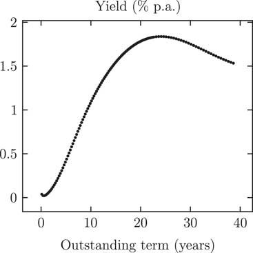
For v(t) we will follow McCulloch (Reference McCulloch1971) and McCulloch (Reference McCulloch1975) and use a spline basis for representing the yields. Note, however, that McCulloch placed his splines with knot points at non-equal distances, whereas we will use equally spaced splines with penalisation as per Eilers and Marx (Reference Eilers and Marx1996); the plotted points in Figure 1 are sufficiently regular that they look like a smooth curve already, so no distortion is introduced by smoothing. In this paper the P-spline smoothing is applied to the yields directly, rather than to the bond prices as in McCulloch (Reference McCulloch1971) and McCulloch (Reference McCulloch1975). The resulting P-spline-smoothed yield curve reproduces all the main features of Figure 1.
3. Model Fitting
We fit models to the data assuming a Poisson distribution for the number of deaths, i.e.
 $$D_{{x,y}} {\rm_~\rm Poisson}\:\left( {\mu _{{x,y}} E_{{x,y}}^{c} } \right)$$
where
 $$E_{{x,y}}^{c} $$
denotes the central exposure to risk at age x last birthday in calendar year y. The Poisson assumption means that the variance of the death counts is equal to the mean, which is not true in practice due to over-dispersion. There are several ways of allowing for this over-dispersion: Li et al. (Reference Li, Hardy and Tan2009) proposed a gamma-distributed heterogeneity parameter which varied by age, while Djeundje and Currie (Reference Djeundje and Currie2011) used a single over-dispersion parameter across all ages and years. However, in this paper we will not make an allowance for over-dispersion for simplicity, as we are primarily interested in comparing the models for μ
x,y
with each other.
$$E_{{x,y}}^{c} $$
denotes the central exposure to risk at age x last birthday in calendar year y. The Poisson assumption means that the variance of the death counts is equal to the mean, which is not true in practice due to over-dispersion. There are several ways of allowing for this over-dispersion: Li et al. (Reference Li, Hardy and Tan2009) proposed a gamma-distributed heterogeneity parameter which varied by age, while Djeundje and Currie (Reference Djeundje and Currie2011) used a single over-dispersion parameter across all ages and years. However, in this paper we will not make an allowance for over-dispersion for simplicity, as we are primarily interested in comparing the models for μ
x,y
with each other.
The models we will fit are the following:
 \hskip -56pt$$\:{\rm Age\hskip-2pt-\hskip-2ptPeriod}\:\quad \log \mu _{{x,y}} {\equals}\alpha _{x} {\plus}\kappa _{y} $$
 $$\:{\rm APC}\;\quad \log \mu _{{x,y}} {\equals}\alpha _{x} {\plus}\kappa _{y} {\plus}\gamma _{{y{\minus}x}} $$
 $$\hskip -45pt\:{\rm Lee\hskip-2pt-\hskip-2ptCarter}\:\quad \log \mu _{{x,y}} {\equals}\alpha _{x} {\plus}\beta _{x} \kappa _{y} $$
 $$\hskip 41pt\:{\rm APCI}\;\quad \log \mu _{{x,y}} {\equals}\alpha _{x} {\plus}\beta _{x} (y{\minus}\bar{y}){\plus}\kappa _{y} {\plus}\gamma _{{y{\minus}x}} $$
where
 $$\bar{y}$$
is the mean over the years 1971–2015. We have selected these models as they are related to each other, but some other models are considered in Appendix F.
$$\bar{y}$$
is the mean over the years 1971–2015. We have selected these models as they are related to each other, but some other models are considered in Appendix F.
Following Brouhns et al. (Reference Brouhns, Denuit and Vermunt2002) we estimate the parameters using the method of maximum likelihood, rather than the singular-value decomposition of Lee and Carter (Reference Lee and Carter1992) or a Bayesian approach. Our focus is on the practical implementation of stochastic models in industry applications, so we estimate
 $$\hat{\kappa }$$
and then, for forecasting, fit a variety of models to
$$\hat{\kappa }$$
and then, for forecasting, fit a variety of models to
 $$\hat{\kappa }$$
treating it as an observed time series. This is preferable to re-estimating κ every time we change the model for it, as a fully Bayesian analysis would require. For a discussion of this practical aspect in insurance applications, see Kleinow and Richards (Reference Kleinow and Richards2016).
$$\hat{\kappa }$$
treating it as an observed time series. This is preferable to re-estimating κ every time we change the model for it, as a fully Bayesian analysis would require. For a discussion of this practical aspect in insurance applications, see Kleinow and Richards (Reference Kleinow and Richards2016).
The Age–Period, APC and APCI models are all linear in the parameters to be estimated, so we will use the algorithm of Currie (Reference Currie2013, pages 87–92) to fit them. The Currie algorithm is a generalisation of the iteratively reweighted least-squares algorithm of Nelder and Wedderburn (Reference Nelder and Wedderburn1972) used to fit generalised linear models (GLMs), but extended to handle models which have both identifiability constraints and smoothing via the penalised splines of Eilers and Marx (Reference Eilers and Marx1996); see Appendix D for an overview. The Lee–Carter model is not linear, but it can be fitted as two alternating linear models as described by Currie (Reference Currie2013, pages 77–80); as with the other three models, constraints and smoothing via penalised splines are applied during the fitting process. Smoothing will be applied to α x and β x , but not to κ y or γ y−x ; smoothing of α x and β x reduces the effective number of parameters and improves the quality of the forecasts by reducing the risk of mortality rates crossing over at adjacent ages; see Delwarde et al. (Reference Delwarde, Denuit and Eilers2007) and Currie (Reference Currie2013). The fitting algorithm is implemented in R (R Core Team, 2013).
4. Smoothing
An important part of modelling is choosing which parameters to smooth. This is not merely an aesthetic consideration – Delwarde et al. (Reference Delwarde, Denuit and Eilers2007) showed how judicious use of smoothing can improve the quality of forecasts, such as by reducing the likelihood of projected mortality rates crossing over at adjacent ages in the future. Figure 2 shows the
 $$\hat{\alpha }_{x} $$
estimates for each of the four models. There is a highly regular, linear-like pattern in each case. We can therefore replace the 55
$$\hat{\alpha }_{x} $$
estimates for each of the four models. There is a highly regular, linear-like pattern in each case. We can therefore replace the 55
 $$\hat{\alpha }_{x} $$
estimates with a smooth curve, or we could even replace them with a straight line for a Gompertz-like version of each model (Gompertz, Reference Gompertz1825). This will have the benefit of reducing the effective dimension of the models, i.e., the effective number of parameters. For smoothing we use the penalised splines of Eilers and Marx (Reference Eilers and Marx1996).
$$\hat{\alpha }_{x} $$
estimates with a smooth curve, or we could even replace them with a straight line for a Gompertz-like version of each model (Gompertz, Reference Gompertz1825). This will have the benefit of reducing the effective dimension of the models, i.e., the effective number of parameters. For smoothing we use the penalised splines of Eilers and Marx (Reference Eilers and Marx1996).
Parameter estimates
 $$\hat{\alpha }_{x} $$
for four unsmoothed models. The α
x
parameters play the same role across all four models, i.e., the average log(mortality) value across 1971–2015, when the constraint
$$\hat{\alpha }_{x} $$
for four unsmoothed models. The α
x
parameters play the same role across all four models, i.e., the average log(mortality) value across 1971–2015, when the constraint
 $$\mathop{\sum}\limits_y \kappa _{y} {\equals}0$$
is applied.
$$\mathop{\sum}\limits_y \kappa _{y} {\equals}0$$
is applied.
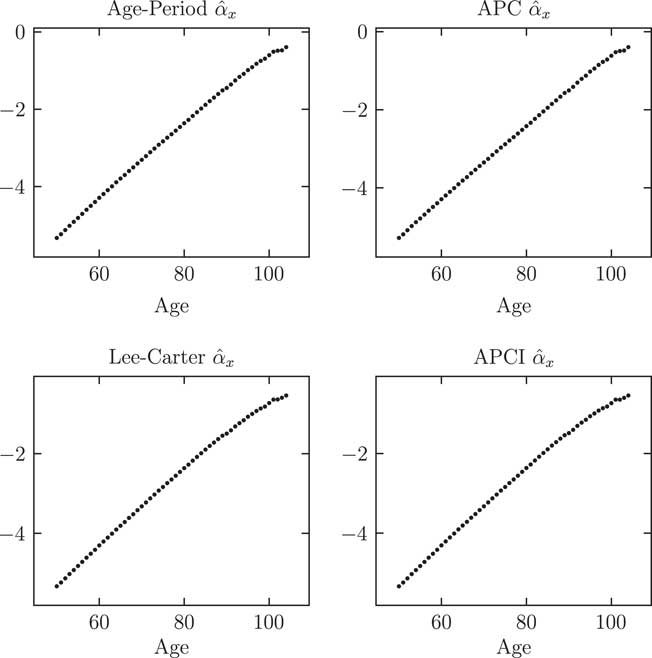
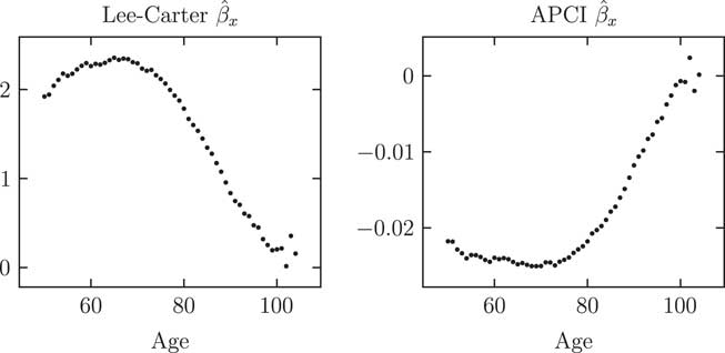
Figure 3 shows the
 $$\hat{\beta }_{x} $$
values for the Lee–Carter and APCI models. Although the pattern of the β
x
values looks different, this arises from the parameterisation of the models. One view of the APCI model is that it separates the linear component of the time trend in the Lee–Carter model and makes κ the residual, non-linear part of the time trend, i.e.
$$\hat{\beta }_{x} $$
values for the Lee–Carter and APCI models. Although the pattern of the β
x
values looks different, this arises from the parameterisation of the models. One view of the APCI model is that it separates the linear component of the time trend in the Lee–Carter model and makes κ the residual, non-linear part of the time trend, i.e.
 $$\beta _{x} \kappa _{y} {\equals}\beta _{x} (\kappa _{y} {\plus}y{\minus}\bar{y}{\minus}y{\plus}\bar{y})$$
 $$\hskip 37pt{\equals}\beta _{x} (y{\minus}\bar{y}){\plus}\beta _{x} (\kappa _{y} {\minus}y{\plus}\bar{y})$$
 $$\hskip 7pt\,\approx\,\beta _{x} (y{\minus}\bar{y}){\plus}\kappa _{y}^{{APCI}} $$
where
 $$\kappa _{y}^{{APCI}} \,\approx\,\beta _{x} (\kappa _{y} {\minus}y{\plus}\bar{y})$$
. Now we see why the β
x
term has a reverse sign under the APCI model, since in the Lee–Carter model κ
y
has a negative slope but in the APCI model
$$\kappa _{y}^{{APCI}} \,\approx\,\beta _{x} (\kappa _{y} {\minus}y{\plus}\bar{y})$$
. Now we see why the β
x
term has a reverse sign under the APCI model, since in the Lee–Carter model κ
y
has a negative slope but in the APCI model
 $$y{\minus}\bar{y}$$
has a positive slope. It would seem more sensible to have
$$y{\minus}\bar{y}$$
has a positive slope. It would seem more sensible to have
 $${\minus}\beta _{x} (y{\minus}\bar{y})$$
in the APCI model to align the parameterisations, but we will stick with the parameterisation of Continuous Mortality Investigation (2017). Figure 3 shows regularity in the
$${\minus}\beta _{x} (y{\minus}\bar{y})$$
in the APCI model to align the parameterisations, but we will stick with the parameterisation of Continuous Mortality Investigation (2017). Figure 3 shows regularity in the
 $$\hat{\beta }_{x} $$
estimates, albeit not as strong as for the
$$\hat{\beta }_{x} $$
estimates, albeit not as strong as for the
 $$\hat{\alpha }_{x} $$
estimates in Figure 2. Again, we can replace the fifty-five
$$\hat{\alpha }_{x} $$
estimates in Figure 2. Again, we can replace the fifty-five
 $$\hat{\beta }_{x} $$
estimates with a smooth curve to reduce the effective dimension of the Lee–Carter and APCI models. The greater variability of the
$$\hat{\beta }_{x} $$
estimates with a smooth curve to reduce the effective dimension of the Lee–Carter and APCI models. The greater variability of the
 $$\hat{\beta }_{x} $$
estimates in Figure 3 shows that smoothing here will make an important contribution to reducing the likelihood of mortality rates crossing over in the forecast; smoothing of the
$$\hat{\beta }_{x} $$
estimates in Figure 3 shows that smoothing here will make an important contribution to reducing the likelihood of mortality rates crossing over in the forecast; smoothing of the
 $$\hat{\beta }_{x} $$
terms for this reason was first proposed by Delwarde et al. (Reference Delwarde, Denuit and Eilers2007). Smoothing the
$$\hat{\beta }_{x} $$
terms for this reason was first proposed by Delwarde et al. (Reference Delwarde, Denuit and Eilers2007). Smoothing the $\hat{\beta }_{x} $
values will therefore both reduce the dimension of the model and improve the forecast quality.
$\hat{\beta }_{x} $
values will therefore both reduce the dimension of the model and improve the forecast quality.
Parameter estimates
 $$\hat{\beta }_{x} $$
for Lee–Carter and APCI models (both unsmoothed). Despite the apparent difference, a switch in sign shows that the β
x
parameters play analogous roles in the Lee–Carter and APCI models, namely an age-related modulation of the response in mortality to the time index
$$\hat{\beta }_{x} $$
for Lee–Carter and APCI models (both unsmoothed). Despite the apparent difference, a switch in sign shows that the β
x
parameters play analogous roles in the Lee–Carter and APCI models, namely an age-related modulation of the response in mortality to the time index
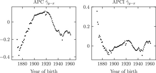
In contrast to Figures 2 and 3, Figures 4 and 5 suggest that smoothing κ and γ is less straightforward. In particular, the
 $$\hat{\kappa }$$
estimates for the APCI model in the lower right panel of Figure 4 do not have a clear trend, in which case smoothing
$$\hat{\kappa }$$
estimates for the APCI model in the lower right panel of Figure 4 do not have a clear trend, in which case smoothing
 $$\hat{\kappa }$$
under the APCI model would make little sense. In Figure 5 the pattern does not look to be regular and well-behaved enough to warrant smoothing, even though it is technically feasible; the repeated changes in direction suggest that extrapolation would be unwise. In both cases we prefer to leave both
$$\hat{\kappa }$$
under the APCI model would make little sense. In Figure 5 the pattern does not look to be regular and well-behaved enough to warrant smoothing, even though it is technically feasible; the repeated changes in direction suggest that extrapolation would be unwise. In both cases we prefer to leave both
 $$\hat{\kappa }$$
and
$$\hat{\kappa }$$
and
 $$\hat{\gamma }$$
unsmoothed so that we can project them using time-series methods. Note that Richards and Currie (Reference Richards and Currie2009) presented a version of the Lee–Carter model with
$$\hat{\gamma }$$
unsmoothed so that we can project them using time-series methods. Note that Richards and Currie (Reference Richards and Currie2009) presented a version of the Lee–Carter model with
 $$\hat{\kappa }$$
smoothed and thus projected using the penalty function.
$$\hat{\kappa }$$
smoothed and thus projected using the penalty function.
Parameter estimates
 $$\hat{\kappa }_{y} $$
for four unsmoothed models. While κ
y
plays a similar role in the Age–Period, Age–Period–Cohort (APC) and Lee–Carter models, it plays a very different role in the APCI model. The APCI
$$\hat{\kappa }_{y} $$
for four unsmoothed models. While κ
y
plays a similar role in the Age–Period, Age–Period–Cohort (APC) and Lee–Carter models, it plays a very different role in the APCI model. The APCI
 $$\hat{\kappa }_{y} $$
estimates are an order of magnitude smaller than in the other models, and with no clear trend. In the APCI model κ
y
is much more of a residual or left-over term, whose values are therefore strongly influenced by structural decisions made elsewhere in the model
$$\hat{\kappa }_{y} $$
estimates are an order of magnitude smaller than in the other models, and with no clear trend. In the APCI model κ
y
is much more of a residual or left-over term, whose values are therefore strongly influenced by structural decisions made elsewhere in the model

Parameter estimates
 $$\hat{\gamma }_{{y{\minus}x}} $$
for Age–Period–Cohort (APC) and APCI models (both unsmoothed). The γ
y−x
values play analogous roles in the APC and APCI models, yet the values taken and the shapes displayed are very different.
$$\hat{\gamma }_{{y{\minus}x}} $$
for Age–Period–Cohort (APC) and APCI models (both unsmoothed). The γ
y−x
values play analogous roles in the APC and APCI models, yet the values taken and the shapes displayed are very different.
We have omitted plots of the
 $$\hat{\alpha }_{x} $$
and
$$\hat{\alpha }_{x} $$
and
 $$\hat{\beta }_{x} $$
estimates in the smoothed models as they are just smoothed-curve versions of Figures 2 and 3. Similarly, we have also omitted plots of
$$\hat{\beta }_{x} $$
estimates in the smoothed models as they are just smoothed-curve versions of Figures 2 and 3. Similarly, we have also omitted plots of
 $$\hat{\kappa }_{y} $$
and
$$\hat{\kappa }_{y} $$
and
 $$\hat{\gamma }_{{y{\minus}x}} $$
under the smoothed models, as they are to all practical purposes identical to Figures 4 and 5. This is an important aspect about smoothing – if it is done appropriately, the smoothing of one parameter vector should not make a major impact on any unsmoothed parameter vectors.
$$\hat{\gamma }_{{y{\minus}x}} $$
under the smoothed models, as they are to all practical purposes identical to Figures 4 and 5. This is an important aspect about smoothing – if it is done appropriately, the smoothing of one parameter vector should not make a major impact on any unsmoothed parameter vectors.
Table 1 summarises our approach to smoothing the various parameters across the four models. The impact of the decision to smooth is shown in the contrast between Tables 2 and 3. We can see that smoothing has little impact on either the forecast time lived or the annuity factors for the Age–Period, Lee–Carter and APCI models. However, smoothing has led to a major change in the central forecast in the case of the APC model; this is due to a different autoregressive, integrated moving average (ARIMA) model being selected as optimal for the κ y terms: ARIMA(0, 1, 2) for the unsmoothed APC model, but ARIMA(3, 2, 0) for the smoothed version. This large change in forecast is an interesting, if extreme, example of the kind of issues discussed in Kleinow and Richards (Reference Kleinow and Richards2016). An ARIMA(p, 1, q) process models the differences in κ y , i.e., a model for improvements, whereas an ARIMA(p, 2, q) process models the rate of change in differences in κ y , i.e., accelerating or decelerating improvements. Smoothing has also improved the fit as measured by the Bayesian information criterion (BIC) – in each case the BIC for a given smoothed model in Table 3 is smaller than the equivalent unsmoothed model in Table 2. This is due to the reduction in the effective number of parameters from the penalisation of the spline coefficients; see equation (21) in Appendix D.
Smoothed and Unsmoothed Parameters
Expected time lived and annuity factors for unsmoothed models, together with the Bayesian Information Criterion (BIC) and Effective Dimension (ED).
The yield curve used to discount future cashflows in the annuity factors is shown in Figure 1.
Expected time lived and annuity factors for smoothed (S) models, together with the Bayesian Information Criterion (BIC) and Effective Dimension (ED).
The yield curve used to discount future cashflows in the annuity factors is shown in Figure 1.
One other interesting aspect of Tables 2 and 3 is the dramatic improvement in overall fit of the APCI model compared to the others. However, it is worth repeating the caution of Currie (Reference Currie2016) that an “oft-overlooked caveat is that it does not follow that an improved fit to data necessarily leads to improved forecasts of mortality”. This was also noted in Kleinow and Richards (Reference Kleinow and Richards2016), where the best-fitting ARIMA process for κ in a Lee–Carter model for UK males led to the greatest parameter uncertainty in the forecast, and thus higher capital requirements under a value-at-risk (VaR) assessment. As we will see in Section 7, although the APCI model fits the data best of the four related models considered, it also produces relatively high capital requirements.
From this point on the models in this paper are smoothed as per Table 1, and the smoothed models will be denoted (S) to distinguish them from the unsmoothed versions.
5. Projections
The κ values will be treated throughout this paper as if they are known quantities, but it is worth noting that this is a simplification. In fact, the
 $$\hat{\kappa }$$
estimates have uncertainty over their true underlying value, especially if they are estimated from the mortality experience of a small population; see, for example, Chen et al. (Reference Chen, Cairns and Kleinow2017). The true κ can be regarded as a hidden process, since we cannot observe κ directly and can only infer likely values given the random variation from realised deaths in a finite population. As a result, the estimated variance of the volatility in any ARIMA process fitted to
$$\hat{\kappa }$$
estimates have uncertainty over their true underlying value, especially if they are estimated from the mortality experience of a small population; see, for example, Chen et al. (Reference Chen, Cairns and Kleinow2017). The true κ can be regarded as a hidden process, since we cannot observe κ directly and can only infer likely values given the random variation from realised deaths in a finite population. As a result, the estimated variance of the volatility in any ARIMA process fitted to
 $$\hat{\kappa }$$
will be an over-estimate, as the estimated
$$\hat{\kappa }$$
will be an over-estimate, as the estimated
 $$\hat{\kappa }$$
values are subject to two sources of variation. There is a parallel here to the concept of a Kalman filter, which models an observable process (the estimated κ) which is itself a realisation of a hidden underlying linear process (the true κ). The Kalman filter therefore allows for two types of noise: measurement error and volatility. In this paper ARIMA models for κ and γ will be estimated using R’s arima() function, which uses a Kalman filter to estimate the underlying parameter values, but assuming that there is no measurement error.
$$\hat{\kappa }$$
values are subject to two sources of variation. There is a parallel here to the concept of a Kalman filter, which models an observable process (the estimated κ) which is itself a realisation of a hidden underlying linear process (the true κ). The Kalman filter therefore allows for two types of noise: measurement error and volatility. In this paper ARIMA models for κ and γ will be estimated using R’s arima() function, which uses a Kalman filter to estimate the underlying parameter values, but assuming that there is no measurement error.
As in Li et al. (Reference Li, Hardy and Tan2009) we will adopt a two-stage approach to mortality forecasting: (i) estimation of the time index, κ
y
, and (ii) forecasting that time index. The practical benefits of this approach over Bayesian methods, particularly with regards to VaR calculations in life-insurance work, are discussed in Kleinow and Richards (Reference Kleinow and Richards2016). The same approach is used for
 $$\gamma _{{y{\minus}x}} $$
. The details of the ARIMA models used are given in Appendix E.
$$\gamma _{{y{\minus}x}} $$
. The details of the ARIMA models used are given in Appendix E.
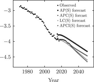
Central projections under each of the four models are shown in Figure 6. The discontinuity between observed and forecast rates for the Age–Period(S) model arises from the lack of age-related modulation of the κ y term – at ages 50–60 there is continuity, at ages 65–75 there is a discontinuity upwards and at ages 85–90 there is a discontinuity downwards. It is for this kind of reason that the Age–Period model is not used in practice for forecasting work.
Observed mortality rates at age 70 and projected rates under Age–Period (smoothed) (AP(S)), Age–Period–Cohort (smoothed) (APC(S)), Lee–Carter (smoothed) (LC(S)) and APCI(S) models
6. Constraints and Cohort Effects
All four of the models in the main body of this paper require identifiability constraints, and the ones used in this paper are detailed in Appendix C. There is a wide choice of alternative constraint systems. For example, R’s gnm() function deletes sufficient columns from the model matrix until it is of full rank and the remaining parameters are uniquely estimable and hence identifiable; see Currie (Reference Currie2016). Cairns et al. (Reference Cairns, Blake, Dowd, Coughlan, Epstein, Ong and Balevich2009) imposed weighted constraints on the
 $$\gamma _{{y{\minus}x}} $$
parameters that performed a dual purpose: (i) acting as identifiability constraints, and (ii) imposing behaviour on
$$\gamma _{{y{\minus}x}} $$
parameters that performed a dual purpose: (i) acting as identifiability constraints, and (ii) imposing behaviour on
 $$\gamma _{{y{\minus}x}} $$
to make forecasting assumptions valid. In explaining their choice of identifiability constraints, Cairns et al. (Reference Cairns, Blake, Dowd, Coughlan, Epstein, Ong and Balevich2009) stated that their choice ensured that the fitted
$$\gamma _{{y{\minus}x}} $$
to make forecasting assumptions valid. In explaining their choice of identifiability constraints, Cairns et al. (Reference Cairns, Blake, Dowd, Coughlan, Epstein, Ong and Balevich2009) stated that their choice ensured that the fitted
 $$\gamma _{{y{\minus}x}} $$
will fluctuate around 0 and will have no discernible linear trend or quadratic curvature.
$$\gamma _{{y{\minus}x}} $$
will fluctuate around 0 and will have no discernible linear trend or quadratic curvature.
However, one consequence of the treatment of corner cohorts described in Appendix B is that it reduces the number of constraints required to uniquely identify parameters in the fitting of the APC and APCI models. Following the rationale of Cairns et al. (Reference Cairns, Blake, Dowd, Coughlan, Epstein, Ong and Balevich2009) in imposing behaviour on
 $$\gamma _{{y{\minus}x}} $$
, both we and Continuous Mortality Investigation (2016b) use the full set of constraints, meaning that both we and Continuous Mortality Investigation (2016b) are using over-constrained models. For the data set of UK males used in this paper, this policy of over-constraining has a much bigger impact on the shape of the parameter values in APCI model than in the APC model.
$$\gamma _{{y{\minus}x}} $$
, both we and Continuous Mortality Investigation (2016b) use the full set of constraints, meaning that both we and Continuous Mortality Investigation (2016b) are using over-constrained models. For the data set of UK males used in this paper, this policy of over-constraining has a much bigger impact on the shape of the parameter values in APCI model than in the APC model.
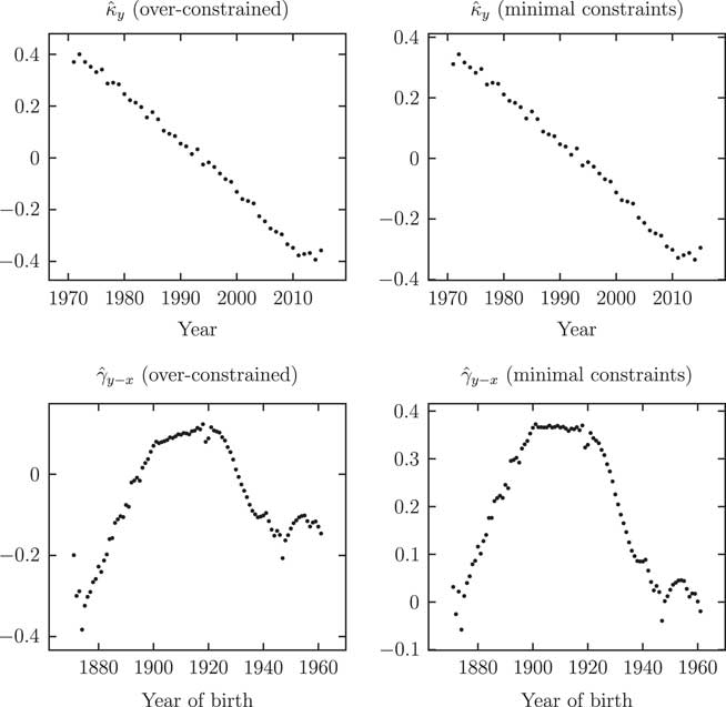
The shape of the APC parameters is largely unaffected by over-constraining, as evidenced by Figure 7. However, it is a matter of concern that the values for
 $$\hat{\kappa }_{y} $$
and
$$\hat{\kappa }_{y} $$
and
 $$\hat{\gamma }_{{y{\minus}x}} $$
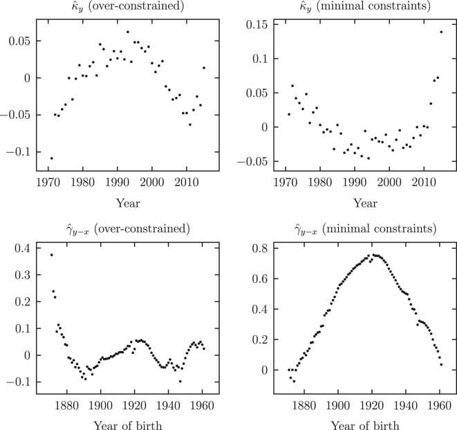
change so much for the APCI model in Figure 8, at least for this data set and with the choice of cohort constraints. In the case of
$$\hat{\gamma }_{{y{\minus}x}} $$
change so much for the APCI model in Figure 8, at least for this data set and with the choice of cohort constraints. In the case of
 $$\hat{\kappa }_{y} $$
, the suspicion is that this term is little more than a residual or left-over in the APCI model. This is a result of the
$$\hat{\kappa }_{y} $$
, the suspicion is that this term is little more than a residual or left-over in the APCI model. This is a result of the
 $$\beta _{x} (y{\minus}\bar{y})$$
term in the APCI model, which picks up the trend that for the other models is present in κ
y
.
$$\beta _{x} (y{\minus}\bar{y})$$
term in the APCI model, which picks up the trend that for the other models is present in κ
y
.
Parameter estimates
 $$\hat{\kappa }_{y} $$
and
$$\hat{\kappa }_{y} $$
and
 $$\hat{\gamma }_{{y{\minus}x}} $$
for the Age–Period–Cohort (smoothed) model: left panels from over-constrained fit, right panels with minimal constraints. The shape of the
$$\hat{\gamma }_{{y{\minus}x}} $$
for the Age–Period–Cohort (smoothed) model: left panels from over-constrained fit, right panels with minimal constraints. The shape of the
 $$\hat{\kappa }_{y} $$
and
$$\hat{\kappa }_{y} $$
and
 $$\hat{\gamma }_{{y{\minus}x}} $$
parameters is largely unaffected by the choice of minimal constraints or over-constraining.
$$\hat{\gamma }_{{y{\minus}x}} $$
parameters is largely unaffected by the choice of minimal constraints or over-constraining.
Parameter estimates
 $$\hat{\kappa }_{y} $$
and
$$\hat{\kappa }_{y} $$
and
 $$\hat{\gamma }_{{y{\minus}x}} $$
for APCI(S) model: left panels from over-constrained fit, right panels with minimal constraints. In contrast to Figure 7, the shape of the parameter estimates is heavily affected by the choice to over-constrain the γ
y−x
parameters.
$$\hat{\gamma }_{{y{\minus}x}} $$
for APCI(S) model: left panels from over-constrained fit, right panels with minimal constraints. In contrast to Figure 7, the shape of the parameter estimates is heavily affected by the choice to over-constrain the γ
y−x
parameters.
The changes in κ
y
and
 $$\gamma _{{y{\minus}x}} $$
from a minimal constraint system to an over-constrained system depend on the nature of the additional constraints that are applied. In the example in Figure 8 it so happens that the constraints are not consistent with γ=0 for corner cohorts. A different set of constraints, rather than those outlined in Appendix C, would lead to different estimated parameter values on the left-hand side of Figure 8 and the changes on the right-hand side of Figure 8 might therefore be made greater or smaller.
$$\gamma _{{y{\minus}x}} $$
from a minimal constraint system to an over-constrained system depend on the nature of the additional constraints that are applied. In the example in Figure 8 it so happens that the constraints are not consistent with γ=0 for corner cohorts. A different set of constraints, rather than those outlined in Appendix C, would lead to different estimated parameter values on the left-hand side of Figure 8 and the changes on the right-hand side of Figure 8 might therefore be made greater or smaller.
When we compare the minimal-constraint fits in Figures 7 and 8, we see that for both models
 $$\gamma _{{y{\minus}x}} $$
approximately follows a quadratic function plus some noise. Due to the additional constraint for the APCI model, the quadratic trend is removed in Figure 8, but only the linear trend is removed in Figure 7. It is then unsurprising that the estimated parameter values change more for the APCI model. However, removing the quadratic trend like this has the advantage of making the γ process in the APCI model look more like a stationary time series, and therefore easier to predict or simulate.
$$\gamma _{{y{\minus}x}} $$
approximately follows a quadratic function plus some noise. Due to the additional constraint for the APCI model, the quadratic trend is removed in Figure 8, but only the linear trend is removed in Figure 7. It is then unsurprising that the estimated parameter values change more for the APCI model. However, removing the quadratic trend like this has the advantage of making the γ process in the APCI model look more like a stationary time series, and therefore easier to predict or simulate.
7. VaR Assessment
Insurers in the United Kingdom and European Union are required to use a 1 year, VaR methodology to assess capital requirements for longevity trend risk. Under Solvency II a VaR99.5 value is required, i.e., insurers must hold enough capital to cover 99.5% of possible changes over one year in the financial impact of mortality forecasts. For a set, S, of possible annuity values arising over the coming year, the VaR99.5 capital requirement would be:
 $${{q(S,99.5\,\%\,){\minus}q(S,50\,\%\,)} \over {q(S,50\,\%\,)}}$$
where q(S,α) is the α-quantile of the set S, i.e., for any randomly selected value in S, s, we have that
 $$\Pr \left( {s\,\lt\,q(S,\alpha )} \right){\equals}\alpha $$
. To generate the set S we use the procedure described in Richards et al. (Reference Richards, Currie and Ritchie2014) to assess long-term longevity trend risk within a one-year framework. The results of this are shown in Table 4.
$$\Pr \left( {s\,\lt\,q(S,\alpha )} \right){\equals}\alpha $$
. To generate the set S we use the procedure described in Richards et al. (Reference Richards, Currie and Ritchie2014) to assess long-term longevity trend risk within a one-year framework. The results of this are shown in Table 4.
Results of Value-at-Risk Assessment
The 99.5% quantiles are estimated by applying the estimator from Harrell and Davis (Reference Harrell and Davis1982) to 5,000 simulations. The ranges given are the 95% confidence intervals computed from the standard error for the Harrell–Davis estimate. The yield curve used to discount future cashflows is shown in Figure 1.
Table 4 shows VaR99.5 capital requirements at age 70, while Figure 9 shows a wide range of ages. The APCI(S) capital requirements appear less smooth and well-behaved than than those for the other models, but the VaR99.5 capital requirements themselves do not appear out of line. We note, however, that the APCI VaR capital requirements exceed the APC(S) and Lee–Carter (S) values at almost every age. How a model’s capital requirements vary with age may be an important consideration for life insurers under Solvency II, such as when calculating the risk margin and particularly for closed (and therefore ageing) portfolios.
VaR99.5 capital-requirement percentages by age for models in Table 4.

To understand how the VaR99.5 capital requirements in Table 4 arise, it is instructive to consider the smoothed densities of the annuity factors at age 70 for each model in Figure 10. Here we can see the reason for the higher capital requirement under the APCI model – there is a relatively wider gap between the median and the 99.5% quantile value.
Densities for annuity factors for age 70 from 2015 for 5,000 simulations under the models in Table 4. The dashed vertical lines show the medians and the dotted vertical lines show the Harrell–Davis estimates for the 99.5% quantiles. The shape of the right-hand tail of the APCI(S) model, and the clustering of values far from the median, leads to the higher VaR99.5 capital requirements in Table 4.
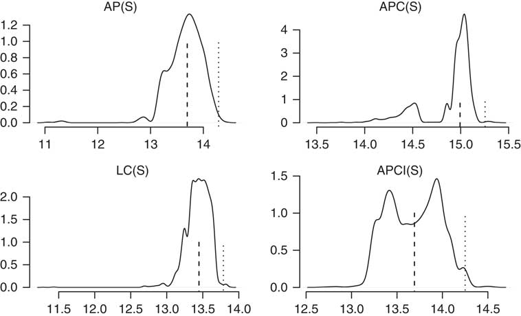
Table 4 shows the impact of model risk in both the median projected annuity factor and the capital requirement. This is a reminder that it is important for practical insurance work to always use a variety of models from different families. Indeed, we note that the best estimate under the APC(S) model in Table 4 is higher than the estimated VaR99.5 reserves for the other models, a phenomenon also observed by Richards et al. (Reference Richards, Currie and Ritchie2014).
8. Conclusions
The APCI model is an interesting addition to the actuarial toolbox. It shares features with the Lee–Carter and APC models and – as with all models – it has its own peculiarities. In the case of the APCI model, the
 $$\hat{\kappa }_{y} $$
estimates for UK males are heavily dependent on whether the model is over-constrained or not. With minimal constraints the
$$\hat{\kappa }_{y} $$
estimates for UK males are heavily dependent on whether the model is over-constrained or not. With minimal constraints the
 $$\hat{\kappa }_{y} $$
estimates in the APCI model for UK male mortality look like a much noisier process than for other models, largely because the linear component of the time trend is accounted for by the
$$\hat{\kappa }_{y} $$
estimates in the APCI model for UK male mortality look like a much noisier process than for other models, largely because the linear component of the time trend is accounted for by the
 $$\beta _{x} (y{\minus}\bar{y})$$
term. On the face of it this raises questions over whether κ
y
should even be kept in the model. However, κ
y
captures non-linear curvature in the trend and period deviations – without it the APCI model would have unrealistically low uncertainty over its projections. With minimal constraints it is also trickier to find a forecasting model for the γ process. Either way, with minimal constraints or not, neither κ
y
nor γ
y−x
look like suitable candidates for smoothing.
$$\beta _{x} (y{\minus}\bar{y})$$
term. On the face of it this raises questions over whether κ
y
should even be kept in the model. However, κ
y
captures non-linear curvature in the trend and period deviations – without it the APCI model would have unrealistically low uncertainty over its projections. With minimal constraints it is also trickier to find a forecasting model for the γ process. Either way, with minimal constraints or not, neither κ
y
nor γ
y−x
look like suitable candidates for smoothing.
In the APCI model the
 $$\hat{\gamma }_{{y{\minus}x}} $$
estimates change dramatically according to whether the model is over-constrained or not. This is not a feature of the APC model, where the shape of the
$$\hat{\gamma }_{{y{\minus}x}} $$
estimates change dramatically according to whether the model is over-constrained or not. This is not a feature of the APC model, where the shape of the
 $$\hat{\gamma }_{{y{\minus}x}} $$
estimates appear relatively robust to the choice to over-constrain or not, at least for this data set for UK males.
$$\hat{\gamma }_{{y{\minus}x}} $$
estimates appear relatively robust to the choice to over-constrain or not, at least for this data set for UK males.
The APCI model fits the data better than the other models considered in this paper, but fit to the data is no guarantee of forecast quality. Interestingly, despite having an improved fit to the data, the APCI model leads to higher capital requirements under a VaR-style assessment of longevity trend risk than most of the other models considered here. These higher requirements vary by age, emphasising that insurers must not only consider multiple models when assessing longevity trend risk, but also the distribution of liabilites by age.
Acknowledgements
The authors thank Alison Yelland, Stuart McDonald, Kevin Armstrong, Yiwei Zhao and an anonymous reviewer for helpful comments. Any errors or omissions remain the responsibility of the authors. All models were fitted using the Projections Toolkit. Graphs were done in R and tikz, while typesetting was done in LATEX. Torsten Kleinow acknowledges financial support from the Actuarial Research Centre (ARC) of the Institute and Faculty of Actuaries through the research programme on Modelling, Measurement and Management of Longevity and Morbidity Risk.
Appendices
A. Integration
We need to evaluate the integrals in equations (1–3). There are several approaches which could be adopted when the function to be integrated can be evaluated at any point, such as adaptive quadrature; see Press et al. (Reference Press, Teukolsky, Vetterling and Flannery2005, page 133) for details of this and other methods. However, since we only have data at integer ages, tp x,y can only be calculated at equally spaced grid points. Since we cannot evaluate the function to be integrated at any point we like, we maximise our accuracy by using the following approximations.
For two points separated by one year we use the Trapezoidal Rule:
 $${\int}_a^{a{\plus}1} f(x)\,\approx\,{1 \over 2}\left[ {f(a){\plus}f(a{\plus}1)} \right]$$
For three points spaced 1 year apart we use Simpson’s Rule:
 $${\int}_a^{a{\plus}2} f(x)\,\approx\,{1 \over 3}\left[ {f(a){\plus}4f\left( {a{\plus}1} \right){\plus}f(a{\plus}2)} \right]$$
For four points spaced one year apart we use Simpson’s 3/8 Rule:
 $${\int}_a^{a{\plus}3} f(x)\,\approx\,{3 \over 8}\left[ {f(a){\plus}3f(a{\plus}1){\plus}3f(a{\plus}2){\plus}f(a{\plus}3)} \right]$$
For five points spaced 1 year apart we use Boole’s Rule:
 $${\int}_a^{a{\plus}4} f(x)\,\approx\,{2 \over {45}}\left[ {7f(a){\plus}32f(a{\plus}1){\plus}12f(a{\plus}2){\plus}32f(a{\plus}3){\plus}7f(a{\plus}4)} \right]$$
To integrate over n equally spaced grid points we first apply Boole’s Rule as many times as possible, then Simpson’s 3/8 Rule, then Simpson’s Rule and then the Trapezoidal Rule for any remaining points at the highest ages.
B. Corner Cohorts
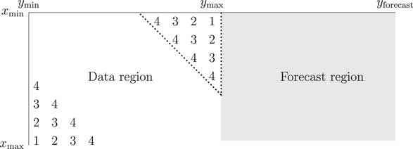
One issue with the APC and APCI models is that the cohort terms can have widely varying numbers of observations, as illustrated in Figure A1; at the extremes, the oldest and youngest cohorts have just a single observation each. A direct consequence of this limited data is that any estimated γ term for the corner cohorts will have a very high variance, as shown in Figure A2. Cairns et al. (Reference Cairns, Blake, Dowd, Coughlan, Epstein, Ong and Balevich2009) dealt with this by simply discarding the data in the triangles in Figure A1, i.e., where a cohort had four or fewer observations. Instead of the oldest cohort having year of birth y min−x max, for example, it becomes c min=y min−x max+4. Similarly, the youngest cohort has year of birth c max=y max−x min−4 instead of y max−x min.
Number of observations for each cohort in the data region
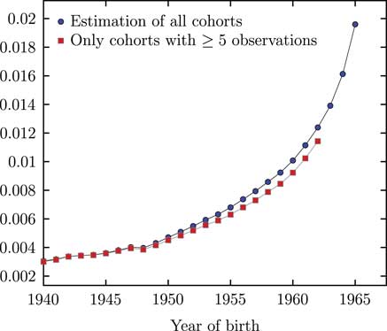
Standard errors of
 $$\hat{\gamma }_{{y{\minus}x}} $$
for APCI(S) model with and without estimation of corner cohorts.
$$\hat{\gamma }_{{y{\minus}x}} $$
for APCI(S) model with and without estimation of corner cohorts.
 $$\hat{\gamma }_{{y{\minus}x}} $$
terms for the cohort cohorts in Figure A1 have very high standard errors; not estimating them has the additional benefit of stabilising the standard errors of those cohort terms we do estimate.
$$\hat{\gamma }_{{y{\minus}x}} $$
terms for the cohort cohorts in Figure A1 have very high standard errors; not estimating them has the additional benefit of stabilising the standard errors of those cohort terms we do estimate.
There is a drawback to the approach of Cairns et al. (Reference Cairns, Blake, Dowd, Coughlan, Epstein, Ong and Balevich2009), namely it makes it harder to compare model fits. We typically use an information criterion to compare models, such as the AIC or BIC. However, this is only valid where the data used are the same. If two models use different data, then their information criteria cannot be compared. This would be a problem for comparing the models in Tables 2, 3 and 12, for example, as the fit for an APC or APCI model could not be compared with the fits for the Age–Period and Lee–Carter models if corner cohorts were only dropped for some models. One approach would be to make the data the same by dropping the corner cohorts for the Age–Period and Lee–Carter fits, even though this is technically unnecessary. This sort of thing is far from ideal, however, as it involves throwing away data and would have to be applied to all sorts of other non-cohort-containing models.
An alternative approach is to use all the data, but to simply not fit cohort terms in the corners of Figure 1. This preserves the easy comparability of information criteria between different model fits. To avoid fitting cohort terms where they are too volatile we simply assume a value of γ=0 where there are four or fewer observations. This means that the same data are used for models with and without cohort terms, and thus that model fits can be directly compared via the BIC. Currie (Reference Currie2013) noted that this had the beneficial side effect of stabilising the variance of the cohort terms which are estimated, as shown in Figure A2.
For projections of γ we forecast not only for the unobserved cohorts, but also for the cohorts with too few observations, i.e., the cohorts in the dotted triangle in Figure A1.
C. Identifiability Constraints
The models in equations (5)–(8) all require identifiability constraints. For the Age–Period model we require one constraint, and we will use the following:
 $$\mathop{\sum}\limits_y \kappa _{y} {\equals}0$$
For the Lee–Carter model we require two constraints. For one of them we will use the same constraint as equation (17), together with the usual constraint on β x from Lee and Carter (Reference Lee and Carter1992):
 $$\mathop{\sum}\limits_x \beta _{x} {\equals}1$$
There are numerous alternative constraint systems for the Lee–Carter model – see Girosi and King (Reference Girosi and King2008), Renshaw and Haberman (Reference Renshaw and Haberman2006) and Richards and Currie (Reference Richards and Currie2009) for examples. The choice of constraint system will affect the estimated parameter values, but will not change the fitted values of
 $$\hat{\mu }_{{x,y}} $$
.
$$\hat{\mu }_{{x,y}} $$
.
For the APC model we require three constraints. For the first one we will use the same constraint as equation (17), together with the following two from Cairns et al. (Reference Cairns, Blake, Dowd, Coughlan, Epstein, Ong and Balevich2009):
 $$\mathop{\sum}\limits_c w_{c} \gamma _{c} {\equals}0$$
 $$\mathop{\sum}\limits_c w_{c} (c{\minus}c_{{{\rm min}}} {\plus}1)\gamma _{c} {\equals}0$$
where w c is the number of times cohort c appears in the data. Continuous Mortality Investigation (2016b) uses unweighted cohort constraints, i.e., w c =1,∀c, but we prefer to use the constraints of Cairns et al. (Reference Cairns, Blake, Dowd, Coughlan, Epstein, Ong and Balevich2009), as they give less weight to years of birth with less data.
For the APCI model we require five constraints. We will use equations (17), (19) and (20), together with the following additional two:
 $$\mathop{\sum}\limits_y (y{\minus}y_{{{\rm min}}} )\kappa _{y} {\equals}0$$
 $$\mathop{\sum}\limits_c w_{c} (c{\minus}c_{{{\rm min}}} {\plus}1)^{2} \gamma _{c} {\equals}0$$
where equation (22) is the continuation of the pattern in equations (19) and (20) established by Cairns et al. (Reference Cairns, Blake, Dowd, Coughlan, Epstein, Ong and Balevich2009).
The number of constraints necessary for a linear model can be determined from the rank of the model matrix. Note that the approach of not fitting γ terms for cohorts with four or fewer observations, as outlined in Appendix B, makes the constraints involving γ unnecessary for identifiability. As in Continuous Mortality Investigation (2016b), this means that the APC and APCI models in this paper are over-constrained, and will thus usually produce poorer fits than would be expected if a minimal constraint system were adopted. Over-constraining has a different impact on the two models: for the APC model it leads to relatively little change in κ, as shown in Figure 7. However, for the APCI model κ is little more than a noise process in the minimally constrained model (see Figure 8), while any pattern in κ from the over-constrained model appears likely to have been caused by the constraints on γ y−x .
D. Fitting Penalised Constrained Linear Models
The Age–Period, APC and APCI models in equations (5), (6) and (8) are Generalized Linear Models (GLMs) with identifiability constraints. We smooth the parameters as described in Table 1. We accomplish the parameter estimation, constraint application and smoothing simultaneously using the algorithm presented in Currie (Reference Currie2013). In this section, we outline the three development stages leading up to this algorithm.
Nelder and Wedderburn (Reference Nelder and Wedderburn1972) defined the concept of a GLM. At its core we have the linear predictor, η, defined as follows:
 $$\eta {\equals}X\theta $$
where X is the model matrix or design matrix and θ is the vector of parameters in the model. For the model to be identifiable we require that the rank of X equals the length of θ; the model of Cairns et al. (Reference Cairns, Blake and Dowd2006) is just such a mortality model (also referred to as M5 in Cairns et al., Reference Cairns, Blake, Dowd, Coughlan, Epstein, Ong and Balevich2009). Nelder and Wedderburn (Reference Nelder and Wedderburn1972) presented an algorithm of iteratively weighted least squares (IWLS), the details of which vary slightly according to (i) the assumption for the distribution of deaths and (ii) the link function connecting the linear predictor to the mean of that distribution. This algorithm finds the values,
 $$\hat{\theta }$$
, which jointly maximise the (log-)likelihood.
$$\hat{\theta }$$
, which jointly maximise the (log-)likelihood.
X can also contain basis splines, which introduces the concept of smoothing and penalisation into the GLM framework; see Eilers and Marx (Reference Eilers and Marx1996). Currie (Reference Currie2013). extended the IWLS algorithm to find the values,
 $$\hat{\theta }$$
, which jointly maximise the penalised likelihood for some given value of the smoothing parameter, λ. The optimum value of λ is determined outside the likelihood framework by minimising an information criterion, such as the BIC:
$$\hat{\theta }$$
, which jointly maximise the penalised likelihood for some given value of the smoothing parameter, λ. The optimum value of λ is determined outside the likelihood framework by minimising an information criterion, such as the BIC:
 $${\rm BIC}{\equals}{\rm Dev}{\plus}\log (n){\rm ED}$$
where n is the number of observations, Dev is the model deviance (McCullagh and Nelder, Reference McCullagh and Nelder1989) and ED is the effective dimension of the model (Hastie and Tibshirani, Reference Hastie and Tibshirani1986). In the single-dimensional case, as λ increases so does the degree of penalisation. The penalised parameters therefore become less free to take values different from their neighbours. The result of increasing λ is therefore to reduce the effective dimension of the model, and so equation (24) balances goodness of fit (measured by the deviance, Dev) against the smoothness of the penalised coefficients (measured via the effective dimension, ED). Currie et al. (Reference Currie, Durban and Eilers2004) and Richards et al. (Reference Richards, Kirkby and Currie2006) used such penalised GLMs to fit smooth, two-dimensional surfaces to mortality grids.
We note that penalisation is applied to parameters which exhibit a smooth and continuous progression, such as the α
x
parameters in equations (5)–(8). If a second-order penalty is applied, as
 $$\lambda \to\infty$$
the smooth curve linking the parameters becomes ever more like a simple straight line, i.e., the effective dimension of α
x
would tend to ED=2. Alternatively, the α
x
could be replaced with two parameters for a simple straight-line function of age. In the case of equations (5)–(8) this would simplify the models to variants of the Gompertz model of mortality (Gompertz, Reference Gompertz1825).
$$\lambda \to\infty$$
the smooth curve linking the parameters becomes ever more like a simple straight line, i.e., the effective dimension of α
x
would tend to ED=2. Alternatively, the α
x
could be replaced with two parameters for a simple straight-line function of age. In the case of equations (5)–(8) this would simplify the models to variants of the Gompertz model of mortality (Gompertz, Reference Gompertz1825).
Many linear mortality models also require identifiability constraints, i.e., the rank of the model matrix is less than the number of parameters to be estimated. The Age–Period, APC and APCI models of the main body of this paper fall into this category: they are all linear, but in each case rank(X)<length(θ). The gap between rank(X) and length(θ) determines the number of identifiability constraints required. To enable simultaneous parameter estimation, smoothing and application of constraints, Currie (2013) extended the concept of the model matrix, X, to the augmented model matrix, X aug, defined as follows:
 $$X_{{{\rm aug}}} {\equals}\left( {\matrix{ X \cr H \cr } } \right)$$
where H is the constraint matrix with the same number of columns as X and where each row of H corresponds to one linear constraint. If rank(X aug)=length(θ), the model is identifiable. If rank(X aug)>length(θ), then the model is over-constrained; see Appendix C. Note that the use of the augmented model matrix, X aug, here restricts H to containing linear constraints.
In this paper we use a Poisson distribution and a log link for our GLMs; this is the canonical link function for the Poisson distribution. This means that the fitted number of deaths is the anti-log of the linear predictor, i.e., E c ×e η . However, Currie (2014) noted that a logit link often provides a better fit to population data. This would make the fitted number of deaths a logistic function of the linear predictor, i.e., E c ×e η /(1+e η ). If the logistic link is combined with the straight-line assumption for α x in equations (5)–(8), this would simplify the models to variants of the Perks model of mortality; see Richards (Reference Richards2008). Currie (Reference Currie2016; Appendix 1) provides R code to implement the logit link for the Poisson distribution for the number of deaths in a GLM. From experience we further suggest specifying good initial parameter estimates to R’s glm() function when using the logit link, as otherwise there can be problems due to very low exposures at advanced ages. The start option in the glm() function can be used for this. In Appendix F we use a logit link to make a M5 Perks model as an alternative to the M5 Gompertz variant using the log link. As can be seen in Table A8, the M5 Perks model fits the data markedly better than the other M5 variants.
E. Projecting κ and γ
A time series is a sequence of elements ordered by the time at which they occur; stationarity is a key concept. Informally, a time series {Y(t)} is stationary if {Y(t)} looks the same at whatever point in time we begin to observe it – see Diggle (Reference Diggle1990, page 13). Usually we make do with the simpler second-order stationarity, which involves the mean and autocovariance of the time series. Let:
 $$\mu (t){\equals}E[Y(t)]$$
 $${\rm Cov}(t,s){\equals}E[\{ Y(t){\minus}\mu (t)\} \{ Y(s){\minus}\mu (s)\} ]$$
be the mean and autocovariance function of the time series. Then the time series is second-order stationary if:
 $$\mu (t){\equals}\mu ,\;\forall t$$
 $${\rm Cov}(t,s){\equals}{\rm Cov}(\,\mid\,t{\minus}s\,\mid\,),\;\:i.e.\;{\rm Cov}(t,s)\;depends\;only\;on\;\,\mid t{\minus}s \mid\,$$
that is, the covariance between Y(t) and Y(s) depends only on their separation in time; see Diggle (Reference Diggle1990, page 58). In practice, when we say a time series is stationary we mean the series is second-order stationary. The assumption of stationarity of the first two moments only is variously known as weak-sense stationarity, wide-sense stationarity or covariance stationarity
The lag operator, L, operates on an element of a time series to produce the previous element. Thus, if we define a collection of time-indexed values {κ t }, then Lκ t =κ t−1. Powers of L mean the operator is repeatedly applied, i.e., L i κ t =κ t−i . The lag operator is also known as the backshift operator, while the difference operator, Δ, is 1−L.
A time series, κ t , is said to be integrated if the differences of order d are stationary, i.e., (1−L) d κ t is stationary.
A time series, κ
t
, is said to be autoregressive of order p if it involves a linear combination of the previous values, i.e.
 $$\left( {1{\minus}\mathop{\sum}\nolimits_{i{\equals}1}^p {\rm ar}_{i} L^{i} } \right)\kappa _{t} $$
, where ar
i
denotes an autoregressive parameter to be estimated. An AR process is stationary if the so-called characteristic polynomial of the process has no unit roots; see Harvey (Reference Harvey1996). For an AR(1) process this is the case if
$$\left( {1{\minus}\mathop{\sum}\nolimits_{i{\equals}1}^p {\rm ar}_{i} L^{i} } \right)\kappa _{t} $$
, where ar
i
denotes an autoregressive parameter to be estimated. An AR process is stationary if the so-called characteristic polynomial of the process has no unit roots; see Harvey (Reference Harvey1996). For an AR(1) process this is the case if
 $${\minus}1\,\lt\,ar_{1} \,\lt\,1_{{}}^{{}} $$
. For empirically observed time series stationary can be tested using unit-root tests.
$${\minus}1\,\lt\,ar_{1} \,\lt\,1_{{}}^{{}} $$
. For empirically observed time series stationary can be tested using unit-root tests.
A time series, κ
t
, is said to be a moving average of order q if the current value can be expressed as a linear combination of the past q error terms, i.e.
 $$\left( {1{\plus}\mathop{\sum}\nolimits_{i{\equals}1}^q {\rm ma}_{i} L^{i} } \right){\epsilon}_{t} $$
, where ma
i
denotes a moving-average parameter to be estimated and {ε
t
} is a sequence of independent, identically distributed error terms with zero mean and common variance,
$$\left( {1{\plus}\mathop{\sum}\nolimits_{i{\equals}1}^q {\rm ma}_{i} L^{i} } \right){\epsilon}_{t} $$
, where ma
i
denotes a moving-average parameter to be estimated and {ε
t
} is a sequence of independent, identically distributed error terms with zero mean and common variance,
 $$\sigma _{{\epsilon}}^{2} $$
. A moving-average process is always stationary.
$$\sigma _{{\epsilon}}^{2} $$
. A moving-average process is always stationary.
A time series, κ t , can be modelled combining these three elements as an ARIMA model (Harvey, Reference Harvey1981) as follows:
 $$\left( {1{\minus}\mathop{\sum}\limits_{i{\equals}1}^p {\rm ar}_{i} L^{i} } \right)\left( {1{\minus}L} \right)^{d} \kappa _{t} {\equals}\left( {1{\plus}\mathop{\sum}\limits_{i{\equals}1}^q {\rm ma}_{i} L^{i} } \right){\varepsilon}_{t} $$
An ARIMA model can be structured with or without a mean value. The latter is simply saying the mean value is set at 0. The behaviour and interpretation of this mean value is dependent on the degree of differencing, i.e., the value of d in ARIMA(p, d, q).
For the Age–Period, APC and Lee–Carter models (but not the APCI model), an ARIMA model for κ with d=1 is broadly modelling mortality improvements, i.e., κ t +1−κ t . It will be appropriate where the rate of mortality improvement has been approximately constant over time, i.e., without pronounced acceleration or deceleration. An ARIMA model with d=1 but no mean will project gradually decelerating improvements. An ARIMA model with d=1 and a fitted mean will project improvements which will gradually tend to that mean value. In most applications the rate at which the long-term mean is achieved is very slow and the curvature in projected values is slight. However, there are two exceptions to this:
∙ Pure moving-average models, i.e., ARIMA(0, d, q) models. With such models the long-term mean will be achieved quickly, i.e., after q+d years.
∙ ARIMA models where the autoregressive component is weak. For example, an ARIMA(1, d, q) model where the ar1 parameter is closer to 0 will also converge to the long-term mean relatively quickly, with the speed of convergence inversely proportional to the absolute value of the ar1 parameter.
For the Age–Period, APC and Lee–Carter models (but not the APCI model), an ARIMA model for κ with d=2 is broadly modelling the rate of change in mortality improvements, not the improvements themselves. Thus, with d=2 we are modelling (κ t + 2−κ t + 1)−(κ t + 1−κ t ). Such a model will be appropriate where the rate of mortality improvement has been accelerating or decelerating over time. An ARIMA model with d=2 and without a mean will project a gradual deceleration of the rate of change in mortality improvements.
To project κ and/or γ in each of the models in the paper, we fit an ARIMA model. We fit ARIMA models with a mean for κ in the Age–Period, APC and Lee–Carter models. We fit ARIMA models without a mean for γ in the APC and APCI models, and also for κ in the APCI model.
The ARIMA parameters, including the mean where required, are estimated using R’s arima(), which estimates ARIMA parameters assuming that κ y and γ y−x are known quantities, rather than the estimated quantities that they really are.
While R’s arima() function returns standard errors, for assessing parameter risk we use the methodology outlined in Kleinow and Richards (Reference Kleinow and Richards2016). The reason for this is that sometimes ARIMA parameter estimates can be borderline unstable, and this can lead to wider confidence intervals for the best-fitting model, as shown in Kleinow and Richards (Reference Kleinow and Richards2016).
To fit an ARIMA model we require to specify the autoregressive order (p), the order of differencing (d) and the order of the moving average (q). For a given level of differencing we fit an ARMA(p, q) model and choose the value of p and q by comparing an information criterion; in this paper we used Akaike’s Information Criterion (Akaike, Reference Akaike1987) with a small-sample correction (AICc). Choosing the order of differencing, d, is trickier, as the data used to fit the ARMA(p, q) model are different when d=1 and d=2: with n observations there are n−1 first differences, but only n−2 second differences. To decide on the ARIMA(p, d, q) model we select the best ARMA(p, q) model for a given value of d using the AICc, then we pick the ARIMA(p, d, q) model with the smallest root mean squared error as per Solo (Reference Solo1984).
The choice of differencing order is thorny: with d=1 we are modelling mortality improvements, but with d=2 we are modelling the rate of change of mortality improvements. The latter can produce very different forecasts, as evidenced by comparing the life expectancy for the APC(S) model in Table 3 (with d=2) with the life expectancy for the APC model in Table 2 (with d=1).
Parameters for Autoregressive, Integrated Moving Average (ARIMA)(1,1,2) process for κ in smoothed Age–Period model
Parameters for Autoregressive, Integrated Moving Average (ARIMA)(1,1,2) process for κ in smoothed Lee–Carter model
Parameters for Autoregressive, Integrated Moving Average (ARIMA)(0,1,2) process for κ in smoothed APC model
Parameters for Autoregressive, Integrated Moving Average (ARIMA)(2,1,0) process for γ in smoothed APC model
For a VaR assessment of in-force annuities we need to simulate sample paths for κ. If we want mortality rates in the upper right triangle of Figure A1, then we also need to simulate sample paths for γ. We use the formulae given in Kleinow & Richards (2016) for bootstrapping the mean (for κ only) and then use these bootstrapped parameter values for the ARIMA process to include parameter risk in the VaR assessment (Tables 5–10).
F. Other Models
In their presentation of a VaR framework for longevity trend risk, Richards et al. (Reference Richards, Currie and Ritchie2014) included some other models not considered in the main body of this paper. For interest we present comparison figures for members of the Cairns–Blake–Dowd family of stochastic projection models. We first consider a model sub-family based on Cairns et al. (Reference Cairns, Blake and Dowd2006) (M5) as follows (Table A6):
 $$g(\mu _{{x,y}} ){\equals}\kappa _{{0,y}} {\plus}w(x)\kappa _{{1,y}} $$
Parameters for Autoregressive, Integrated Moving Average (ARIMA)(1,1,2) process for κ in smoothed APCI model

Parameters for Autoregressive, Integrated Moving Average (ARIMA)(2,1,0) process for γ in smoothed APCI model
Definition of M5 Family Under Equation (31)
for some functions g() and w() where κ 0 and κ 1 form a bivariate random walk with drift. The three members of the M5 family used here are defined in Table A7, with the results in Tables A8 and A9. We also consider two further models from Cairns et al. (Reference Cairns, Blake, Dowd, Coughlan, Epstein, Ong and Balevich2009). First, M6:
 $$\log \mu _{{x,y}} {\equals}\kappa _{{0,y}} {\plus}(x{\minus}\bar{x})\kappa _{{1,y}} {\plus}\gamma _{{y{\minus}x}} $$
Model M6 in equation (32) needs two identifiability constraints and we use equations (19) and (20). As with the M5 family, κ 0 and κ 1 form a bivariate random walk with drift and γ is projected using an ARIMA model (as done for the APC and APCI models). We also consider M7 from Cairns et al. (Reference Cairns, Blake, Dowd, Coughlan, Epstein, Ong and Balevich2009):
 $$\log \mu _{{x,y}} {\equals}\kappa _{{0,y}} {\plus}(x{\minus}\bar{x})\kappa _{{1,y}} {\plus}{\plus}\left( {(x{\minus}\bar{x})^{2} {\minus}\hat{\sigma }^{2} } \right)\kappa _{{2,y}} {\plus}\gamma _{{y{\minus}x}} $$
where
 $$\hat{\sigma }^{2} {\equals}{1 \over {n_{x} }}\mathop{\sum}\nolimits_{i{\equals}1}^{n_{x} } (x_{i} {\minus}\bar{x})^{2} $$
. Model M7 in equation (33) needs three identifiability constraints and we use equations (19), (20) and (22). κ
0, κ
1 and κ
2 form a trivariate random walk with drift and γ is projected using an ARIMA model (as done for the APC and APCI models). As with the APC and APCI models, M6 and M7 do not need all these constraints with our treatment of corner cohorts described in Appendix B. Thus, M6 and M7 here are also over-constrained.
$$\hat{\sigma }^{2} {\equals}{1 \over {n_{x} }}\mathop{\sum}\nolimits_{i{\equals}1}^{n_{x} } (x_{i} {\minus}\bar{x})^{2} $$
. Model M7 in equation (33) needs three identifiability constraints and we use equations (19), (20) and (22). κ
0, κ
1 and κ
2 form a trivariate random walk with drift and γ is projected using an ARIMA model (as done for the APC and APCI models). As with the APC and APCI models, M6 and M7 do not need all these constraints with our treatment of corner cohorts described in Appendix B. Thus, M6 and M7 here are also over-constrained.
Expected time lived and annuity factors for unsmoothed models, together with Bayesian Information Criterion (BIC) and Effective Dimension (ED)
Results of Value-at-Risk assessment for models in Table A8

Comparing Table A8 with Tables 2 and 3 we can see that the stochastic version of the APCI model produces similar expected time lived and temporary annuity factors to most models, apart from the APC and M6 models. This suggests that the best-estimate forecasts under the APCI model are consistent and not extreme.
Comparing Table A9 with Table 4 we can see that, while the AP(S) and APCI(S) models produce the largest VaR99.5 capital requirements at age 70, these are not extreme outliers.
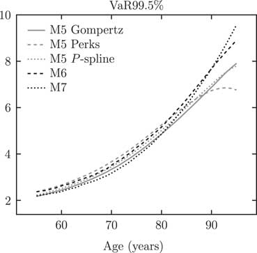
A comparison of Table 4 with the equivalent figures in Richards et al. (Reference Richards, Currie and Ritchie2014, Table 4) shows considerable differences in VaR99.5 capital at age 70. There are two changes between Richards et al. (Reference Richards, Currie and Ritchie2014) and this paper that drive these differences. The first change is that Richards et al. (Reference Richards, Currie and Ritchie2014) discounted cashflows using a flat 3% per annum, whereas in this paper we discount cashflows using the yield curve in Figure 1. The second change lies in the data: in this paper we use UK-wide data for 1971–2015 , whereas Richards et al. (Reference Richards, Currie and Ritchie2014) used England and Wales data for 1961–2010. There are three important sub-sources of variation buried in this change in the data: the first is that the population estimates for 1961–1970 are not as reliable as the estimates which came after 1970; the second is that the data used in this paper include revisions to pre-2011 population estimates following the 2011 census; and the third is that mortality experience after 2010 has been unusual and is not in line with trend. The combined effect of these changes to the discount function and the data has led to the VaR99.5 capital requirements at age 70 for the models in Table A9 being around 0.5% less than for the same models in Richards et al. (Reference Richards, Currie and Ritchie2014, Table 4). However, a comparison between Figures 9 and A3 shows that these results are strongly dependent on age. As in Richards et al. (Reference Richards, Currie and Ritchie2014), this means that it is insufficient to consider a few model points for a VaR assessment – insurer capital requirements not only need to be informed by different projection models, but they must take account of the age distribution of liabilities.
VaR99.5 capital requirements by age for models in Table A8
G. Differences compared to Continuous Mortality Investigation approach
In this paper we present a stochastic implementation of the APCI model proposed by Continuous Mortality Investigation (2016b). This is the central difference between the APCI model in this paper and its original implementation in Continuous Mortality Investigation (2016a, 2016b). However, there are some other differences of note and they are listed in this section as a convenient overview.
As per Cairns et al. (Reference Cairns, Blake, Dowd, Coughlan, Epstein, Ong and Balevich2009) our identifiability constraints for γ y−x weight each parameter according to the number of times it appears in the data, rather than assuming equal weight as in Continuous Mortality Investigation (2016b, page 91). As with Continuous Mortality Investigation (2016b) our APC and APCI models are over-constrained (see Appendix C and section 6).
For cohorts with four or fewer observed values we do not estimate a γ term – see Appendix B. In contrast, Continuous Mortality Investigation (2016a, pages 27–28) adopts a more complex approach to corner cohorts, involving setting the cohort term to the nearest available estimated term.
For smoothing α x and β x we have used the penalised splines of Eilers and Marx (Reference Eilers and Marx1996), rather than the difference penalties in Continuous Mortality Investigation (2016b). Our penalties on α x and β x are quadratic, whereas Continuous Mortality Investigation (2016b) uses cubic penalties. Unlike Continuous Mortality Investigation (2016b) we do not smooth κ y or γ y−x . We also determine the optimal level of smoothing by minimising the BIC, whereas Continuous Mortality Investigation (2016b) smooths by user judgement.
As described in Section 3, for parameter estimation we use the algorithm presented in Currie (Reference Currie2013). This means that constraints and smoothing are an integral part of the estimation, rather than separate steps applied in Continuous Mortality Investigation (2016b, page 15).
Unlike Continuous Mortality Investigation (2016b) we make no attempt to adjust the exposure data.
For projections we use ARIMA models for both κ y and γ y−x , rather than the deterministic targeting approach of Continuous Mortality Investigation (2016b, pages 31–35). Unlike Continuous Mortality Investigation (2016b) we do not attempt to break down mortality improvements into age, period and cohort components, nor do we have a long-term rate to target and nor do we have any concept of a “direction of travel”(Continuous Mortality Investigation, 2016b, page 14).
H. Suggestions for Further Research
There were many other things which could have been done in this paper, but for which there was not the time available. We list some of them here in case others are interested in doing so:
∙ Female lives. To illustrate our points, and to provide comparable figures to earlier papers such as Richards et al. (Reference Richards, Currie and Ritchie2014) and Kleinow and Richards (Reference Kleinow and Richards2016), we used the data for males. However, both insurers and pension schemes have material liabilities linked to female lives, and it would be interesting to explore the application of the APCI model to data on female lives.
∙ Back-testing. It would be interesting to see how the APCI model performs against other models in back-testing, i.e., fit the models to first part of the data set and see how the resulting forecasts compare to the latter part of the data.
∙ Sensitivity testing. Some models are sensitive to the range of ages selected or the period covered. It would be interesting to know how sensitive the APCI model is to such changes.
∙ Canonical correlation. Models with both period and cohort terms, such as the APC and APCI models, usually have these terms projected as if they are independent. However, such terms are usually correlated, making the assumption of independence at best a simplifying assumption for convenience. It would be interesting to compare the correlations of κ and γ for the APC and APCI models. Joint models for κ and γ could be considered.
∙ Over-dispersion. To fit the models, both we and Continuous Mortality Investigation (2017, page 5) assume that the number of deaths follows a Poisson distribution, i.e., that the variance is equal to the mean. However, in practice death counts are usually over-dispersed, i.e., the variance is greater than the mean.


 Open access