


1 Introduction
The enhanced mixing that results from the amplification of turbulence across a shock wave can be critical in applications such as hypersonic propulsion (supersonic combustion ramjets) and inertial confinement fusion. The canonical shock–turbulence interaction (STI) configuration has been extensively studied theoretically, experimentally and through numerical simulations. However, few studies have concentrated on quantifying the effects of the interaction on scalar mixing, in particular as the relevant physical parameters and regime of the interaction are changed, which is the focus of the present work.
Theoretical approaches to study STI include linear interaction analysis (LIA) (Moore Reference Moore1953; Ribner Reference Ribner1953, Reference Ribner1954; Livescu & Ryu Reference Livescu and Ryu2016; Jackson, Kapila & Hussaini Reference Jackson, Kapila and Hussaini1990; Jackson, Hussaini & Ribner Reference Jackson, Hussaini and Ribner1993; Wouchuk, Huete & Velikovich Reference Wouchuk, Huete and Velikovich2009; Quadros, Sinha & Larsson Reference Quadros, Sinha and Larsson2016a,Reference Quadros, Sinha and Larssonb) and rapid distortion theory (RDT) (Lele Reference Lele1992; Cambon, Coleman & Mansour Reference Cambon, Coleman and Mansour1993; Jacquin, Cambon & Blin Reference Jacquin, Cambon and Blin1993; Kitamura et al. Reference Kitamura, Nagata, Sakai, Sasoh and Ito2016). More recently, dimensional and similarity analyses were put forward based on a quasi-equilibrium assumption of instantaneous local adjustment of the shock, seen as a collection of infinitesimal laminar shocks (see Donzis Reference Donzis2012a,Reference Donzisb; Chen Reference Chen2018). In the last two decades, a number of developments have made LIA suitable for the analysis of more complex physics, including mixing, chemical reactions and real gas effects (Griffond Reference Griffond2005, Reference Griffond2006; Huete, Sánchez & Williams Reference Huete, Sánchez and Williams2013, Reference Huete, Sánchez and Williams2014; Hejranfar & Rahmani Reference Hejranfar and Rahmani2019).
Shock-driven mixing enhancement has been observed in experiments (Andreopoulos, Agui & Briassulis Reference Andreopoulos, Agui and Briassulis2000). In the study of the effects of shock propagation on the properties of a random medium, Hesselink & Sturtevant (Reference Hesselink and Sturtevant1988) observed enhanced mixing in the shock-processed, strongly compressed fluid. Marble, Hendricks & Zukoski (Reference Marble, Hendricks and Zukoski1989) found faster mixing by baroclinic vorticity in the interaction of weak oblique shocks and cylindrical jets of hydrogen in air. Menon (Reference Menon1989) observed an accelerated spreading of shear layers downstream of interactions with shock waves, indicative of better mixing. Experiments have also confirmed theoretical LIA predictions on the amplification of small-scale turbulence across the shock (Barre, Alem & Bonnet Reference Barre, Alem and Bonnet1996; Agui, Briassulis & Andreopoulos Reference Agui, Briassulis and Andreopoulos2005; Andreopoulos Reference Andreopoulos2008), concluding that the flows downstream of shocks become more vortex dominated than their upstream counterparts (Andreopoulos Reference Andreopoulos2008).
Numerical simulation, mostly direct numerical simulation (DNS), has become commonplace in the study of STI, complementing experiments and theory. Linear interaction analysis predictions of turbulence kinetic energy (TKE) and transverse vorticity variance amplification, and decreased turbulence length scales across the shock have been confirmed in direct numerical simulations (Lee, Lele & Moin Reference Lee, Lele and Moin1993, Reference Lee, Lele and Moin1994; Ryu & Livescu Reference Ryu and Livescu2014). Likewise, simulations have confirmed the saturation of TKE amplification for Mach numbers larger than 3 (Lee, Lele & Moin Reference Lee, Lele and Moin1997), which could impose limits on achievable shock-induced mixing enhancements for increasing shock strength. But simulations have also elucidated nonlinear effects that cannot be predicted by LIA, such as the rapid postshock TKE evolution and the role of upstream acoustic/vorticity/entropy fluctuations and temperature–velocity correlations on postshock TKE amplification and turbulence length scales (Hannappel & Friedrich Reference Hannappel and Friedrich1995; Mahesh, Lele & Moin Reference Mahesh, Lele and Moin1997; Jamme et al. Reference Jamme, Cazalbou, Torres and Chassaing2002). Different STI regimes have been identified through parametric DNS studies to depend on the relative strength of the incoming turbulence and the shock, characterized by the ratio  $M_{t}/(M-1)$ (Larsson & Lele Reference Larsson and Lele2009; Donzis Reference Donzis2012b; Larsson, Bermejo-Moreno & Lele Reference Larsson, Bermejo-Moreno and Lele2013) or $Re_{\unicode[STIX]{x1D706}}^{-1/2}(M_{t}/(M-1)$ (Donzis Reference Donzis2012a). In the ‘wrinkled-shock’ regime, the shock is simply corrugated by the turbulence, which is in turn amplified across; in the ‘broken-shock’ regime, the shock topology is modified by the appearance of ‘shock holes’ where the shock locally vanishes; in the ‘vanished’ regime, turbulence quantities do not present amplification across the shock but a monotonic decay. Lower fidelity simulation approaches, such as large-eddy simulations (LES) (Bermejo-Moreno, Larsson & Lele Reference Bermejo-Moreno, Larsson and Lele2010; Hickel, Egerer & Larsson Reference Hickel, Egerer and Larsson2014; Braun, Pullin & Meiron Reference Braun, Pullin and Meiron2019) and Reynolds (or Favre) averaged Navier–Stokes (RANS) simulations (Sinha, Mahesh & Candler Reference Sinha, Mahesh and Candler2003; Quadros & Sinha Reference Quadros and Sinha2016; Schwarzkopf et al. Reference Schwarzkopf, Livescu, Baltzer, Gore and Ristorcelli2016) have emerged in the last two decades.
Studies of scalar mixing in the canonical STI configuration are scarce in comparison with other compressible flow configurations, such as compressible homogeneous isotropic turbulence (Pan & Scannapieco Reference Pan and Scannapieco2010, Reference Pan and Scannapieco2011; Ni Reference Ni2015, Reference Ni2016; Danish, Suman & Girimaji Reference Danish, Suman and Girimaji2016) and the shock-driven Richtmyer–Meshkov instability (Brouillette Reference Brouillette2002; Lombardini, Pullin & Meiron Reference Lombardini, Pullin and Meiron2012; Orlicz et al. Reference Orlicz, Balasubramanian, Vorobieff and Prestridge2015; Desjardins et al. Reference Desjardins, Merritt, Flippo, Kline, Di Stefano, DeVolder, Doss, Fierro, Randolph and Schmidt2018; Reese et al. Reference Reese, Ames, Noble, Oakley, Rothamer and Bonazza2018). Tian et al. (Reference Tian, Jaberi, Li and Livescu2017) analysed the effects of density variations on STI and mixing by comparing single- and two-fluid cases using shock-capturing DNS. Faster increase of turbulence stretching and an increased scalar dissipation rate across the shock were identified as the causes for better mixing enhancement for multi-fluid mixing. Boukharfane, Bouali & Mura (Reference Boukharfane, Bouali and Mura2018) compared the streamwise evolution of scalar variance and its dissipation rate between the shocked and unshocked cases, and observed an increase of scalar dissipation rate (SDR) across the shock. They also related the increase of SDR with the change of alignments across the shock. These pioneering studies of scalar mixing in STI were however limited in the Reynolds number as well as shock and turbulence Mach numbers of the interactions considered, which were all in the wrinkled-shock regime. Besides the limited number of studies on scalar mixing under STI, other works have investigated compressibility effects on mixing (Pantano & Sarkar Reference Pantano and Sarkar2002; Vaghefi & Madnia Reference Vaghefi and Madnia2015; Karimi & Girimaji Reference Karimi and Girimaji2016; Jahanbakhshi & Madnia Reference Jahanbakhshi and Madnia2016; Arun et al. Reference Arun, Sameen, Srinivasan and Girimaji2019; Yu & Lu Reference Yu and Lu2019). Although not focused on passive scalars, these investigations have identified flow patterns that are favoured and dominate dissipation in locally compressed regions, relevant to STI.
Building upon Larsson et al. (Reference Larsson, Bermejo-Moreno and Lele2013) and Gao et al. (Reference Gao, Bermejo-Moreno, Larsson, Fu and Lele2018), our present work uses shock-capturing DNS to study passive scalar mixing in the canonical STI configuration under a wider range of physical parameters than previously explored. Wrinkled- and broken-shock regimes are considered for different mean and turbulence Mach numbers, Reynolds number and Schmidt number. The objective is to elucidate, through parametric studies, the streamwise evolution across the shock wave and in the downstream relaxation region of dominant scalar mixing quantities in relation to changes of the background turbulence. The datasets generated from these simulations, including full volumetric fields as well as processed data, are available for download from the corresponding authors.
2 Methodology
2.1 Numerical setup, governing equations and numerical scheme
Shock-capturing direct numerical simulations are used to solve the conservative form of the equations of mass, momentum and total energy conservation of a Newtonian, calorically perfect gas, complemented with transport equations for passive scalars:
 $$\begin{eqnarray}\displaystyle & \displaystyle \unicode[STIX]{x2202}_{t}\unicode[STIX]{x1D70C}+\unicode[STIX]{x2202}_{j}(\unicode[STIX]{x1D70C}u_{j})=0, & \displaystyle\end{eqnarray}$$
 $$\begin{eqnarray}\displaystyle & \displaystyle \unicode[STIX]{x2202}_{t}\unicode[STIX]{x1D70C}u_{i}+\unicode[STIX]{x2202}_{j}(\unicode[STIX]{x1D70C}u_{j}u_{i})=\unicode[STIX]{x2202}_{j}\unicode[STIX]{x1D70E}_{ij}, & \displaystyle\end{eqnarray}$$
 $$\begin{eqnarray}\displaystyle & \displaystyle \unicode[STIX]{x2202}_{t}(\unicode[STIX]{x1D70C}e_{T})+\unicode[STIX]{x2202}_{j}(\unicode[STIX]{x1D70C}u_{j}e_{T})=\unicode[STIX]{x2202}_{j}(u_{i}\unicode[STIX]{x1D70E}_{ij})-\unicode[STIX]{x2202}_{j}q_{j}, & \displaystyle\end{eqnarray}$$
 $$\begin{eqnarray}\displaystyle & \displaystyle \unicode[STIX]{x2202}_{t}\unicode[STIX]{x1D70C}\unicode[STIX]{x1D719}_{\unicode[STIX]{x1D6FC}}+\unicode[STIX]{x2202}_{j}(\unicode[STIX]{x1D70C}u_{j}\unicode[STIX]{x1D719}_{\unicode[STIX]{x1D6FC}})=\unicode[STIX]{x2202}_{j}(\unicode[STIX]{x1D70C}D_{\unicode[STIX]{x1D6FC}}\unicode[STIX]{x2202}_{j}\unicode[STIX]{x1D719}_{\unicode[STIX]{x1D6FC}}). & \displaystyle\end{eqnarray}$$
 Here Einstein summation convention is used for Roman subscripts,  $\unicode[STIX]{x2202}_{t}=\unicode[STIX]{x2202}/\unicode[STIX]{x2202}t$, $\unicode[STIX]{x2202}_{j}=\unicode[STIX]{x2202}/\unicode[STIX]{x2202}x_{j}$, $\unicode[STIX]{x1D70C}$ is the density, $u_{i}$ is the $i$th component of the velocity ( $i=1,2,3$), $e_{T}=e+\frac{1}{2}u_{i}u_{i}$ is the total energy per unit mass ( $e=c_{v}T$ is the internal energy per unit mass, $c_{v}$ is the specific heat capacity at constant volume and $T$ is the temperature), and $\unicode[STIX]{x1D719}_{\unicode[STIX]{x1D6FC}}$ is the $\unicode[STIX]{x1D6FC}$th passive scalar ( $\unicode[STIX]{x1D6FC}=1,\ldots ,M$). Fourier’s law is used to express the conduction heat flux as $q_{j}=-\unicode[STIX]{x1D705}\unicode[STIX]{x2202}_{j}T$, where $\unicode[STIX]{x1D705}$ is the thermal conductivity, chosen such that the Prandtl number $Pr=c_{p}\unicode[STIX]{x1D707}/\unicode[STIX]{x1D705}$ equals 0.7, with $c_{p}$ the specific heat capacity at constant pressure. The stress tensor is defined as $\unicode[STIX]{x1D70E}_{ij}=-p\unicode[STIX]{x1D6FF}_{ij}+\unicode[STIX]{x1D70F}_{ij}$, where $p$ is thermodynamic pressure, $\unicode[STIX]{x1D70F}_{ij}=2\unicode[STIX]{x1D707}(\unicode[STIX]{x1D61A}_{ij}-\unicode[STIX]{x1D61A}_{kk}\unicode[STIX]{x1D6FF}_{ij}/3)$ is the viscous stress tensor, $\unicode[STIX]{x1D61A}_{ij}=\frac{1}{2}(\unicode[STIX]{x2202}_{j}u_{i}+\unicode[STIX]{x2202}_{i}u_{j})$ is the strain-rate tensor and $\unicode[STIX]{x1D707}$ is the dynamic viscosity, which follows the power law $\unicode[STIX]{x1D707}=\unicode[STIX]{x1D707}_{ref}(T/T_{ref})^{3/4}$, with reference viscosity and temperature, $\unicode[STIX]{x1D707}_{ref}$ and $T_{ref}$, respectively. A zero volumetric viscosity has been assumed. The ideal gas law, $p=\unicode[STIX]{x1D70C}RT$, is used to relate static thermodynamic variables in terms of the gas constant, $R$.
$R$.
Reynolds and Favre averages of any flow quantity,  $f$, are denoted by $\bar{f}$ and $\widetilde{f}=\overline{\unicode[STIX]{x1D70C}f}/\overline{\unicode[STIX]{x1D70C}}$, respectively, with corresponding fluctuations defined as $f^{\prime }=f-\overline{f}$ and $f^{\prime \prime }=f-\widetilde{f}$. Averaging is done spatially over the statistically homogeneous transverse directions ( $y=x_{2}$ and $z=x_{3}$) and temporally, since the flow becomes statistically stationary after an initial transient, by adequately setting the outflow back pressure.
The relevant dimensionless parameters of STI are the mean flow (or shockwave) Mach number,  $M=\widetilde{u}_{1,u}/\widetilde{c}$, the turbulence Mach number, $M_{t}=\sqrt{3}u_{rms}^{\prime }/\widetilde{c}$, and the Taylor microscale Reynolds number, $Re_{\unicode[STIX]{x1D706}}=\bar{\unicode[STIX]{x1D70C}}u_{rms}^{\prime }\unicode[STIX]{x1D706}/\bar{\unicode[STIX]{x1D707}}$, where $\unicode[STIX]{x1D706}=[\overline{u_{2}^{\prime }u_{2}^{\prime }}/\overline{(\unicode[STIX]{x2202}_{2}u_{2})^{2}}]^{1/2}$ is the Taylor microscale, $u_{rms}^{\prime }=(\overline{u_{i}^{\prime }u_{i}^{\prime }}/3)^{1/2}$ is the r.m.s. velocity fluctuation and $c$ is the local speed of sound. Another Reynolds number is considered, $Re_{L}=\overline{\unicode[STIX]{x1D70C}}u_{rms}^{\prime }L/\overline{\unicode[STIX]{x1D707}}$, based on the dissipation-based length scale characterizing large eddies, $L_{\unicode[STIX]{x1D716}}=K^{3/2}/\unicode[STIX]{x1D716}$, where $K=\widetilde{u_{i}^{\prime \prime }u_{i}^{\prime \prime }}/2$ is the specific TKE and $\unicode[STIX]{x1D716}=\overline{\unicode[STIX]{x1D70F}_{ij}\unicode[STIX]{x1D61A}_{ij}}/\overline{\unicode[STIX]{x1D70C}}$ its rate of dissipation. Values of these dimensionless parameters reported in this work (see table 1) are determined immediately upstream of the unsteady shock region of each STI simulation. Diffusion of each passive scalar is characterized by the Schmidt number, $Sc_{\unicode[STIX]{x1D6FC}}=\unicode[STIX]{x1D70C}D_{\unicode[STIX]{x1D6FC}}/\unicode[STIX]{x1D707}$, assumed constant in each simulation.
Simulation cases, line styles and symbols (for postshock state) used in figures.

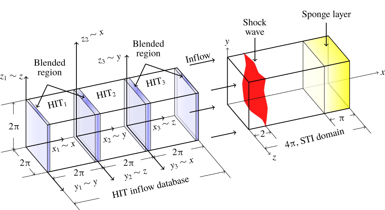
The computational domain for all STI simulations is a rectangular box of size  $(L_{x},L_{y},L_{z})=(4\unicode[STIX]{x03C0}\times 2\unicode[STIX]{x03C0}\times 2\unicode[STIX]{x03C0})$ (see figure 1). The governing equations are discretized on rectilinear, Cartesian grids, uniformly spaced in the transverse directions, and stretched in the mean streamwise direction ( $x=x_{1}$) to increase the resolution near the average shock location. For all simulation cases, $\unicode[STIX]{x0394}x_{2,3}/\unicode[STIX]{x0394}x_{1,s}=2.4$, where $\unicode[STIX]{x0394}x_{2,3}$ is the grid spacing in the transverse ( $y$ and $z$) directions, and $\unicode[STIX]{x0394}x_{1,s}$ is the grid spacing in the streamwise direction immediately after the shock.
Problem setup of STI and blended homogeneous isotropic turbulence (HIT) precursor simulations.
A solution-adaptive numerical method is employed (Larsson & Lele Reference Larsson and Lele2009) that combines a fifth-order weighted essentially non-oscillatory (WENO) scheme with HLL flux splitting near shocks, and a sixth-order central difference scheme in the split form of Ducros et al. (Reference Ducros, Laporte, Souleres, Guinot, Moinat and Caruelle2000) elsewhere. Near-shock regions where WENO is applied are identified as satisfying  $-\unicode[STIX]{x1D703}>1.2\unicode[STIX]{x1D714}_{k}\unicode[STIX]{x1D714}_{k}$, where $\unicode[STIX]{x1D703}=S_{kk}=\unicode[STIX]{x2202}_{k}u_{k}$ is the dilatation, $\unicode[STIX]{x1D714}_{k}\unicode[STIX]{x1D714}_{k}$ is the enstrophy and $\unicode[STIX]{x1D714}_{i}=\unicode[STIX]{x1D716}_{ijk}\unicode[STIX]{x2202}_{j}u_{k}$ is the vorticity. The equations are advanced in time using a fourth-order, four-stage explicit Runge–Kutta scheme. Inflow and outflow boundaries along the streamwise direction use summation by parts operators with simultaneous approximation terms (Svärd & Nordström Reference Svärd and Nordström2014). A sponge layer is used in the STI simulations for $x\in [x_{sp},x_{max}]=[3\unicode[STIX]{x03C0},4\unicode[STIX]{x03C0}]$ to effectively damp acoustic reflections generated at the outflow boundary, preventing upstream propagation into the subsonic region of the domain. To obtain a statistically stationary shock, the back pressure at the outflow plane, $p_{b}$, is specified following Larsson & Lele (Reference Larsson and Lele2009). Periodic boundary conditions are imposed in the transverse directions.
Precursor simulations of decaying homogeneous isotropic turbulence (DHIT) with transport of passive scalars are performed in a periodic box of size  $(2\unicode[STIX]{x03C0})^{3}$. These precursor simulations provide turbulence databases that will be superimposed at the inflow plane of the STI simulations to the mean advection velocity by means of Taylor’s hypothesis. The uniform, isotropic grid spacing in each DHIT simulation is dictated by the transverse resolution of the corresponding STI simulation that will use the inflow dataset. Decaying homogeneous isotropic turbulence simulations follow Larsson et al. (Reference Larsson, Bermejo-Moreno and Lele2013), extended to include passive scalars with initial spectra $E(k)\propto k^{4}\text{e}^{-2k^{2}/k_{0}^{2}}$ and $k_{0}=4$. The resulting initial passive scalar fields have zero mean and unitary variance. Decaying homogeneous isotropic turbulence simulations are run until reaching the targeted $M_{t}$ and $Re_{\unicode[STIX]{x1D706}}$, accounting for decay in the STI upstream of the unsteady shock region. The turbulence is assumed fully developed once the velocity derivative skewness stabilizes around $-0.5$ and the dissipation-based length scale, $L_{\unicode[STIX]{x1D716}}$, increases with time.
To obtain an inflow database sufficiently long to allow for the computation of statistically converged time averages in the STI simulation, snapshots from multiple realizations of DHIT with the same physical parameters ( $M_{t}$, $Re_{\unicode[STIX]{x1D706}}$ and $Sc_{\unicode[STIX]{x1D6FC}}$) but different initial conditions are blended following Larsson (Reference Larsson2009). In addition, from each DHIT snapshot (box), two additional boxes, obtained by a series of rotations, are subsequently blended.
2.2 Simulation cases
In table 1 we present a summary of the simulations performed in this study, varying  $Re_{\unicode[STIX]{x1D706}}$ between ${\approx}40$ (cases $A$–
$A$– $H$) and ${\approx}70$ ( $I$–
$I$– $K$),
$K$),  $M$ from 1.28 to 5.0, and $M_{t}$ from 0.09 to 0.42, which covers a wider parameter space than previously investigated (Tian et al. Reference Tian, Jaberi, Li and Livescu2017; Boukharfane et al. Reference Boukharfane, Bouali and Mura2018). Wrinkled- and broken-shock regimes are thus considered in these simulations, according to the criterion that $M_{t}/(M-1)\gtrapprox 0.6$ is required for the broken-shock regime (see Donzis Reference Donzis2012b; Larsson et al. Reference Larsson, Bermejo-Moreno and Lele2013). Simulation cases $A$–
$A$– $H$ include passive scalars with $Sc=0.5$, 1 and 2, whereas cases $I$–
$I$– $K$ consider $Sc=1$ only.
After an initial transient that accounts for adjustments to the back pressure to obtain a statistically stationary state, statistics are collected over a time period  $L_{input}/\widetilde{u}_{1,u}$, or $k_{0}\widetilde{u}_{1,u}t_{stats}=24\unicode[STIX]{x03C0}$ in dimensionless form. Cases $B$ and $F$, along with other coarser-resolution simulations not shown in table 1, are used for grid-convergence analyses described in the supplementary material available at https://doi.org/10.1017/jfm.2020.292. Simulations with a resolution of $1280\times 384\times 384$ ( $2400\times 1024\times 1024$) are already grid converged for $Re_{\unicode[STIX]{x1D706}}\approx 40$ (70). At this resolution, $k_{max}\unicode[STIX]{x1D702}_{B,d}>1.1$, where $\unicode[STIX]{x1D702}_{B,d}$ is the Batchelor scale immediately downstream of the shock, for the three values of $Sc$ considered. For all simulation cases, once the statistically stationary state is reached, the average shock is located $k_{0}\unicode[STIX]{x0394}x\approx 8$ behind the inflow boundary, where the grid resolution is highest.
3 Shock-normal statistics
In this section we focus on the streamwise evolution of scalar mixing statistics averaged on transverse planes and in time. To compare results from different simulations in the figures to follow, for each case: (1) the streamwise origin is shifted to the start of the unsteady shock region; (2) the streamwise coordinate is rescaled by the dissipation-based length scale taken immediately upstream of the unsteady shock region,  $L_{\unicode[STIX]{x1D716},u}$; (3) the unsteady shock region is either highlighted by a grey shade and a horizontal line segment marking its width, or removed for better comparison of the effective jumps of flow quantities across the averaged unsteady shock regions; (4) when the unsteady shock regions are removed, symbols mark the postshock location for each case, following table 1.
3.1 Reynolds stress, vorticity variance anisotropy and relevant streamwise locations
Streamwise profiles of Favre-averaged streamwise Reynolds stresses (a,b) and vorticity variance anisotropy (c,d) for different simulation cases. Each curve in (a,b) has been normalized by the value immediately upstream of the unsteady shock region. Grey shaded regions and horizontal line segments in (a,b) mark the extent of the unsteady shock region for each case, using the corresponding line style. All unsteady shock regions are removed in (c,d) for a clearer comparison among cases. Vertical segments starting from the horizontal axis indicate the location of  $x_{\hat{\unicode[STIX]{x1D714}}_{x}}$. $M$,
$M$,  $M_{t}$ and $Re_{\unicode[STIX]{x1D706}}$ values for each case are given in parentheses in the legend following table 1.
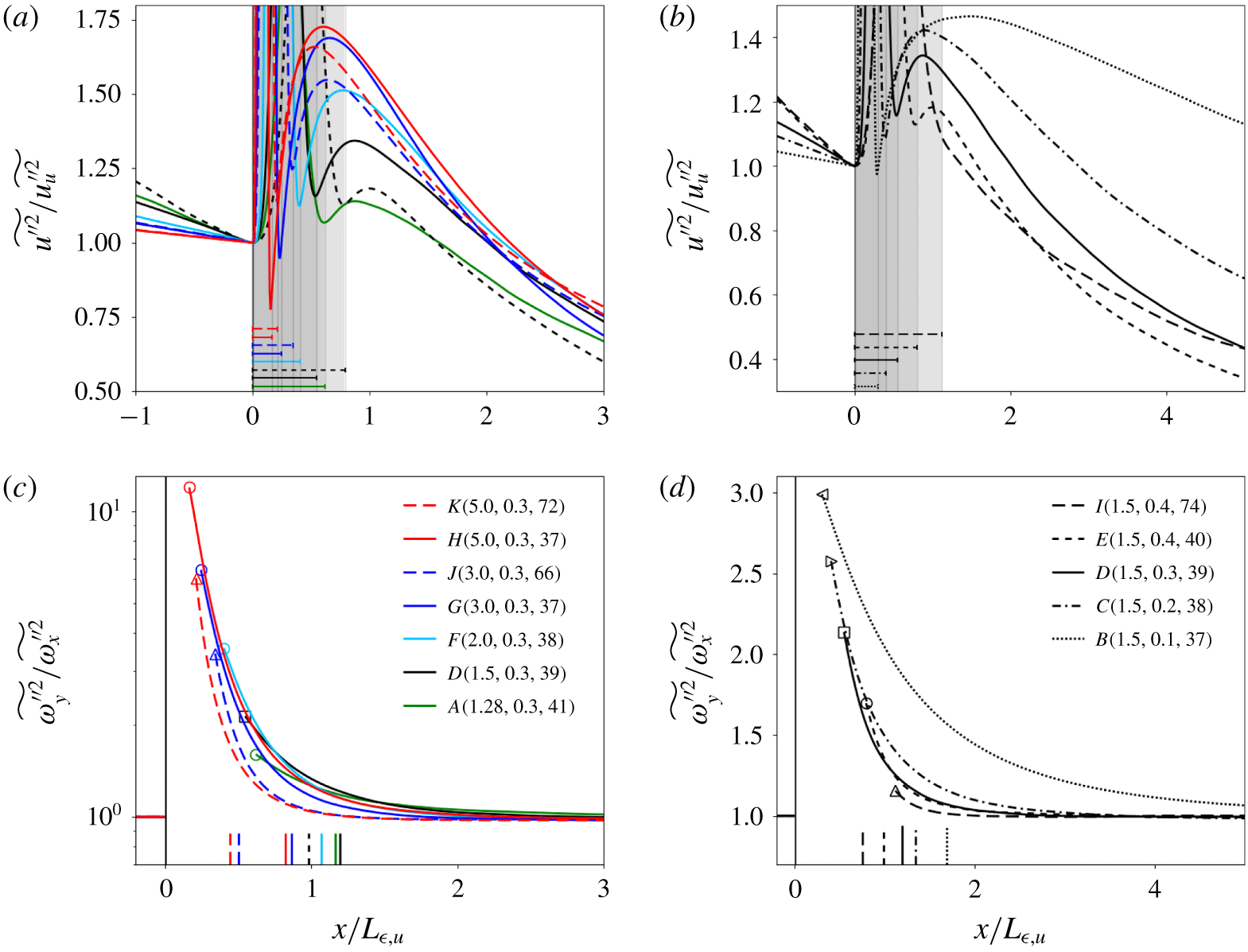
In figure 2(a,b) we show averaged profiles of streamwise Reynolds stresses,  $R_{xx}=\widetilde{u^{\prime \prime 2}}$. For each simulation case, $R_{xx}$ first peaks in the region of shock unsteadiness, generally followed by a second peak farther downstream (outside the unsteady shock region) that results from an acoustic-to-vortical energy transfer (Lee et al. Reference Lee, Lele and Moin1993; Larsson & Lele Reference Larsson and Lele2009). We define the averaged preshock, $x_{pre}$, and postshock, $x_{post}$, locations of each simulation by the first two local minima found in the streamwise profile of $R_{xx}$, respectively. The unsteady shock region lies in between these preshock and postshock locations, as marked by the greyed areas and the horizontal line segments in figure 2(a,b). The width of the unsteady region decreases with $M$, and increases with $M_{t}$ and $Re_{\unicode[STIX]{x1D706}}$. The peak of $R_{xx}$ downstream of the shock increases in magnitude with $M$, tending toward saturation for $M>3$, and decreases with $Re_{\unicode[STIX]{x1D706}}$ and $M_{t}$, which also bring it closer to the shock. For case $I$, with $(M,M_{t},Re_{\unicode[STIX]{x1D706}})=(1.5,0.4,74)$, the unsteady shock region is the widest and encloses the region of acoustic-to-vortical energy transfer, such that there is no local minimum of $R_{xx}$ immediately downstream of the shock. The postshock location for this case $I$ is defined instead by the discontinuous change in slope of $R_{xx}$ (figure 2b).
The streamwise location downstream of the shock where the streamwise vorticity variance reaches its maximum is denoted by  $x_{\hat{\unicode[STIX]{x1D714}}_{x}}$. We define the location of recovery of small-scale isotropy, $x_{iso}$, at the streamwise location downstream of the shock where the vorticity variance anisotropy, $\widetilde{\unicode[STIX]{x1D714}_{y}^{\prime \prime 2}}/\widetilde{\unicode[STIX]{x1D714}_{x}^{\prime \prime 2}}$, recovers to a value of 1.01 (figure 2c,d). Note that the small-scale anisotropy is highest immediately downstream of the shock, increasing for larger $M$, and smaller $M_{t}$ and $Re_{\unicode[STIX]{x1D706}}$. In contrast with $R_{xx}$, the anisotropy does not saturate for the range of $M$ considered here. Higher $Re_{\unicode[STIX]{x1D706}}$ leads to a faster recovery of small-scale isotropy.
3.2 Scalar variance
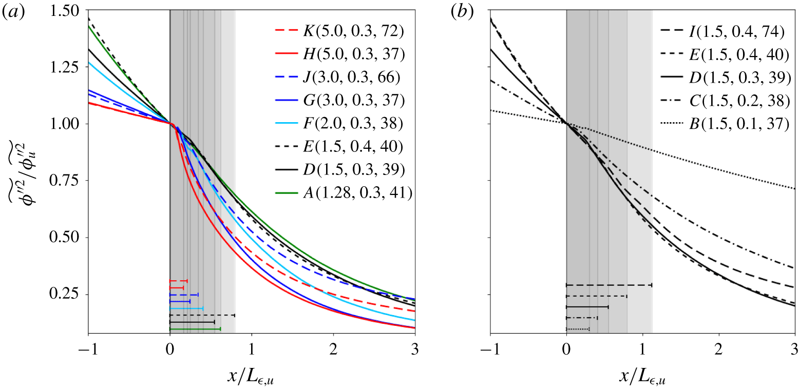
Whereas there is no local jump of passive scalar variance across the instantaneous shock, averaging results into an effective jump across the unsteady shock region due to its finite width (figure 3). The effective jump is defined as the difference between the  $x_{post}$ and $x_{pre}$ values. The Mach number $M$ has a nearly negligible influence on this effective jump of scalar variance, as the reduced unsteady shock width is balanced by a steeper decay rate across the shock. The latter, evidenced by the increased negative slope of the profiles, results from a larger scalar dissipation rate (see § 3.3) and a smaller mean velocity downstream of the shock. Larger $M_{t}$ increases shock corrugation, widens the unsteady shock region, and produces a larger effective jump of scalar variance across the shock. Larger $Re_{\unicode[STIX]{x1D706}}$ slows down the decay rate of normalized scalar variance downstream of the shock, a consequence of the reduced jump of scalar dissipation rate that will be shown in § 3.3.
Streamwise profiles of Favre-averaged scalar variance for (a) cases with the same  $M_{t}$ and (b) cases with the same $M$.
$M$.  $Sc=1$. Each curve is normalized by the value immediately upstream of the unsteady shock region, which is greyed out and marked, for each case, by a horizontal segment with the same line style as the corresponding curve.
3.3 Scalar variance budgets
The transport equation for the Favre-averaged passive scalar variance,  $\widetilde{\unicode[STIX]{x1D719}^{\prime \prime }\unicode[STIX]{x1D719}^{\prime \prime }}$, is
 $$\begin{eqnarray}\displaystyle \unicode[STIX]{x2202}_{t}\left(\overline{\unicode[STIX]{x1D70C}}\widetilde{\unicode[STIX]{x1D719}^{\prime \prime }\unicode[STIX]{x1D719}^{\prime \prime }}\right)+\underbrace{\widetilde{u}_{i}\unicode[STIX]{x2202}_{i}\left(\overline{\unicode[STIX]{x1D70C}}\widetilde{\unicode[STIX]{x1D719}^{\prime \prime }\unicode[STIX]{x1D719}^{\prime \prime }}\right)}_{L1} & = & \displaystyle -\underbrace{\overline{\unicode[STIX]{x1D70C}\unicode[STIX]{x1D719}^{\prime \prime }\unicode[STIX]{x1D719}^{\prime \prime }}\unicode[STIX]{x2202}_{i}\widetilde{u}_{i}}_{{\mathcal{A}}}-\underbrace{2\overline{\unicode[STIX]{x1D70C}u_{i}^{\prime \prime }\unicode[STIX]{x1D719}^{\prime \prime }}\unicode[STIX]{x2202}_{i}\widetilde{\unicode[STIX]{x1D719}}}_{{\mathcal{B}}}-\underbrace{\unicode[STIX]{x2202}_{i}\left(\overline{\unicode[STIX]{x1D70C}u_{i}^{\prime \prime }\unicode[STIX]{x1D719}^{\prime \prime }\unicode[STIX]{x1D719}^{\prime \prime }}\right)}_{{\mathcal{C}}}\nonumber\\ \displaystyle & & \displaystyle +\,\underbrace{2\unicode[STIX]{x2202}_{i}\left(\overline{\unicode[STIX]{x1D70C}D\unicode[STIX]{x1D719}^{\prime \prime }\unicode[STIX]{x2202}_{i}\unicode[STIX]{x1D719}}\right)}_{{\mathcal{D}}}-\underbrace{2\overline{\unicode[STIX]{x1D70C}D\left(\unicode[STIX]{x2202}_{i}\unicode[STIX]{x1D719}^{\prime \prime }\right)^{2}}}_{{\mathcal{E}}}-\underbrace{2\overline{\unicode[STIX]{x1D70C}D\left(\unicode[STIX]{x2202}_{i}\unicode[STIX]{x1D719}^{\prime \prime }\right)\unicode[STIX]{x2202}_{i}\widetilde{\unicode[STIX]{x1D719}}}}_{{\mathcal{F}}},\nonumber\\ \displaystyle & & \displaystyle\end{eqnarray}$$
 where  $D$ is the diffusivity of scalar $\unicode[STIX]{x1D719}$. The local time derivative vanishes once statistical stationarity is reached. The right-hand side includes the dilatational term, ${\mathcal{A}}$, proportional to the dilatation of the Favre-averaged mean velocity; production term, ${\mathcal{B}}$, proportional to the Favre-averaged mean scalar gradient; turbulent diffusion term, ${\mathcal{C}}$; molecular diffusion term, ${\mathcal{D}}$; (turbulent) scalar variance dissipation rate terms, ${\mathcal{E}}$ and ${\mathcal{F}}$. For all cases considered, terms ${\mathcal{B}}$, ${\mathcal{D}}$ and ${\mathcal{F}}$ have a negligible contribution outside the unsteady shock region, and are not shown. The convection of scalar variance by Favre-averaged mean velocity ( $L1$) and the dilatational term ( ${\mathcal{A}}$) can be combined into a conservative (divergence-like) flux term for scalar variance. Thus, the integral of the remaining terms on the right-hand side ( ${\mathcal{C}}$ and ${\mathcal{E}}$) between two streamwise locations then equals the change of scalar variance multiplied by the streamwise momentum.
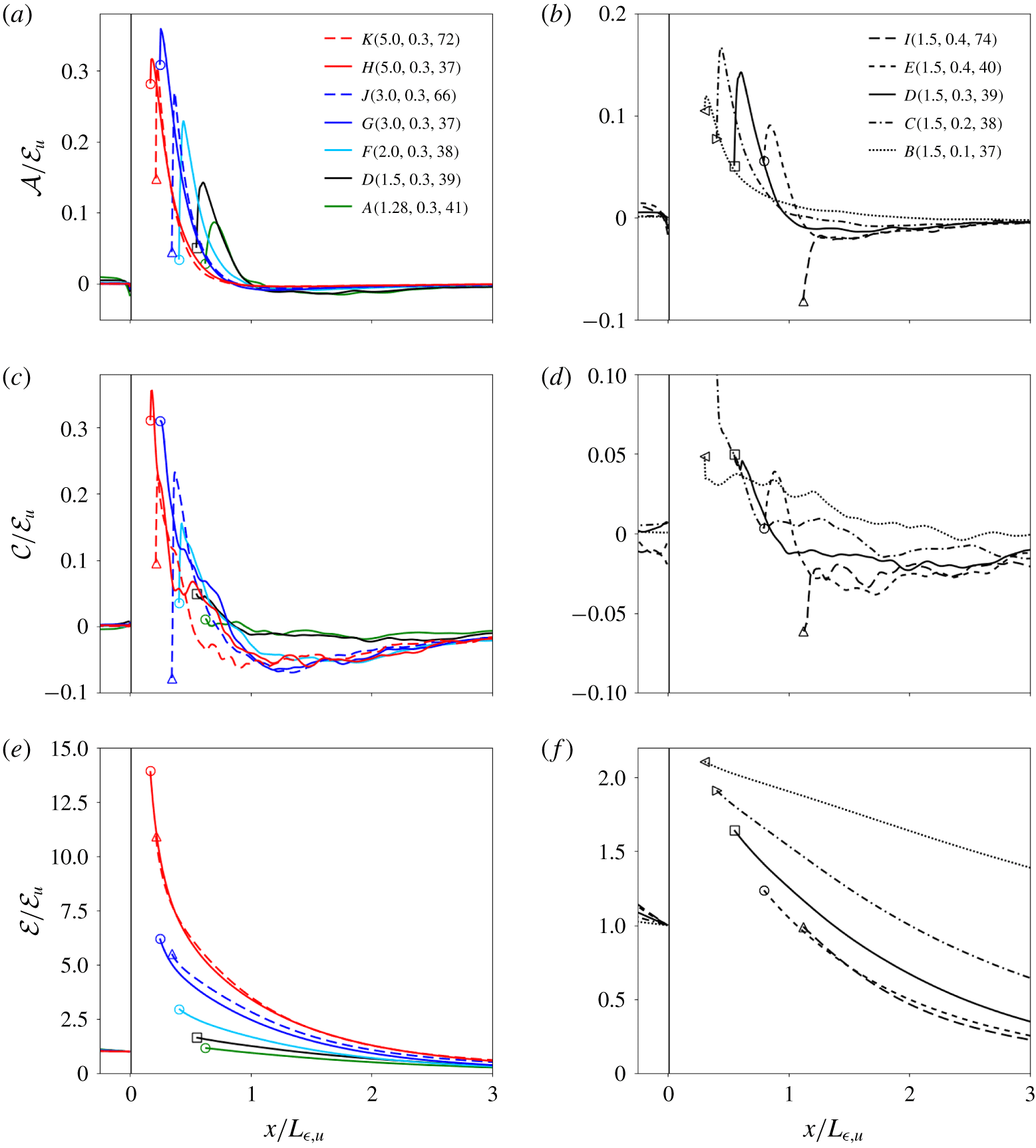
In figure 4 we show streamwise profiles of the dilatational term  ${\mathcal{A}}$, the turbulent diffusion term ${\mathcal{C}}$ and the scalar dissipation rate term ${\mathcal{E}}$. The latter dominates, in agreement with Tian et al. (Reference Tian, Jaberi, Li and Livescu2017), while all three terms increase across the shock. Tian et al. (Reference Tian, Jaberi, Li and Livescu2017) did not perform a parametric study of different terms in (3.1), while Boukharfane et al. (Reference Boukharfane, Bouali and Mura2018) only studied the effects of $M$ (for 1.7, 2.0 and 2.3) on the scalar dissipation term. Dilatational and turbulent diffusion terms reach about ten percent of the scalar dissipation rate term downstream of the shock, in contrast to the results of Tian et al. (Reference Tian, Jaberi, Li and Livescu2017), who found these two terms to be negligible for the mixing of passive scalars, but not for multi-fluid mixing. Our present simulations predict the dilatational and turbulent diffusion terms to be also significant in the mixing of passive scalars, more so for larger $M$ and smaller $Re_{\unicode[STIX]{x1D706}}$. Boukharfane et al. (Reference Boukharfane, Bouali and Mura2018) also observed a non-negligible turbulent diffusion term. The dilatational term peaks shortly downstream of the unsteady shock region. The normalized peak increases with $M$ for $M\leqslant 3$ and slightly decreases for larger $M$. Downstream of the shock, a rapid decay of the dilatational and turbulent diffusion terms follows along a streamwise distance shorter than $L_{\unicode[STIX]{x1D716},u}$. The two terms become slightly negative and recover to negligible values approximately $3L_{\unicode[STIX]{x1D716},u}$ behind the shock. For increasing $M_{t}$, the peak of initial decay is embedded in the wider unsteady shock region (e.g. case $I$ in the broken-shock regime).
Streamwise profiles of non-negligible terms in the transport equation of scalar variance for cases with the same  $M_{t}$ (a,c,e) and cases with the same $M$ (b,d,f). Each curve is normalized by the value immediately upstream of the unsteady shock region (removed for clarity). The preshock location is offset to be at $x=0$ for all cases, and the postshock location, $x_{post}$, is marked with symbols, (a,b) dilatational term; (c,d) turbulent diffusion term; (e,f) dissipation rate of scalar variance.
The effective jump of scalar dissipation rate  ${\mathcal{E}}$ across the shock monotonically increases with $M$ (in agreement with Boukharfane et al. (Reference Boukharfane, Bouali and Mura2018)), and decreases with $M_{t}$ and $Re_{\unicode[STIX]{x1D706}}$, showing no sign of saturation up to $M=5$. Larger $Re_{\unicode[STIX]{x1D706}}$ results in a lower effective jump of scalar dissipation across the shock. To decouple the effect of increased density and viscosity across the shock for cases with different $M$, we introduce a scaled scalar dissipation, $\hat{\unicode[STIX]{x1D712}}={\mathcal{E}}/\overline{2\unicode[STIX]{x1D70C}D}=\overline{\unicode[STIX]{x1D70C}D(\unicode[STIX]{x2202}_{i}\unicode[STIX]{x1D719}^{\prime \prime })^{2}}/\overline{\unicode[STIX]{x1D70C}D}$. This quantity, plotted in figure 5, also shows increasing jump with $M$ across the unsteady shock region, with no signs of saturation. A faster downstream decay is also observed as $M$ increases, whereas larger $Re_{\unicode[STIX]{x1D706}}$ mainly lowers the postshock value. The wider shock region brought in by increased $M_{t}$ leads to effective jumps of $\hat{\unicode[STIX]{x1D712}}/\hat{\unicode[STIX]{x1D712}}_{u}$ below unity for cases in the broken-shock regime. It is expected that as $M_{t}$ is further increased, possibly entering the ‘vanished (shock) regime’, amplification of scalar-related quantities will be progressively reduced, eventually leading to a decay across the shock, as seen for turbulence quantities in Chen & Donzis (Reference Chen and Donzis2019).
Streamwise profiles of scaled scalar dissipation rate,  $\hat{\unicode[STIX]{x1D712}}$, for (a) cases with the same $M_{t}$ and (b) cases with the same $M$. Each curve is normalized by the value immediately upstream of the unsteady shock region (removed for clarity). Symbols mark the postshock location, $x_{post}$. Legend as in figure 4.

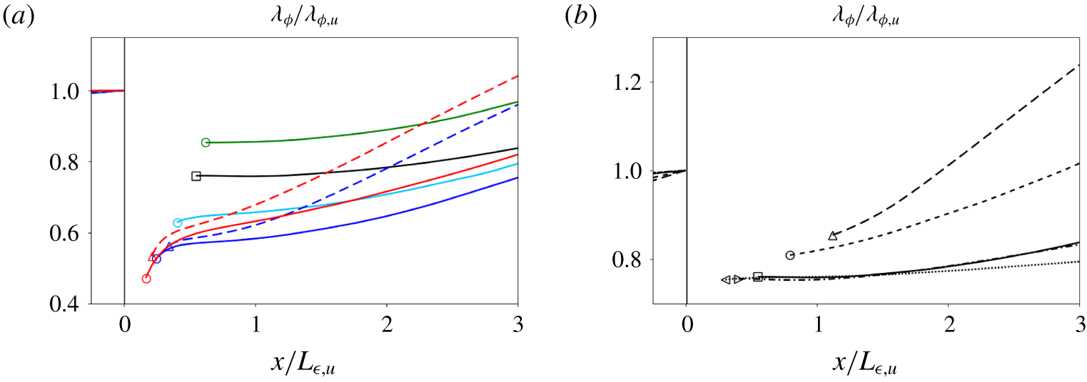
3.4 Scalar Taylor-like microscale
In figure 6 we show the influence of  $M$,
$M$,  $M_{t}$ and $Re_{\unicode[STIX]{x1D706}}$ on the scalar Taylor-like microscale, defined as $\unicode[STIX]{x1D706}_{\unicode[STIX]{x1D719}}=(\widetilde{\unicode[STIX]{x1D719}^{\prime \prime }\unicode[STIX]{x1D719}^{\prime \prime }}/\hat{\unicode[STIX]{x1D712}})^{1/2}$. Across the shock, $\unicode[STIX]{x1D706}_{\unicode[STIX]{x1D719}}$ decreases, more so for increasing $M$ and decreasing $Re_{\unicode[STIX]{x1D706}}$. Downstream of the unsteady shock region, $\unicode[STIX]{x1D706}_{\unicode[STIX]{x1D719}}$ grows at a rate that increases with $M$ and $Re_{\unicode[STIX]{x1D706}}$. Cases with relatively low $M$ (1.28 and 1.5) show a monotonic growth rate, with a nearly uniform $\unicode[STIX]{x1D706}_{\unicode[STIX]{x1D719}}$ for downstream distances below approximately $L_{\unicode[STIX]{x1D716},\text{u}}$. Cases with larger $M$ (
$M$ ( ${\approx}2$–5) show a non-monotonic growth rate, with a fast growth very close to the unsteady shock region ( $x<L_{\unicode[STIX]{x1D716},u}/3$), followed by a slowdown and a subsequent acceleration. Cases in the wrinkled-shock regime share a similar effective jump and downstream recovery of the normalized $\unicode[STIX]{x1D706}_{\unicode[STIX]{x1D719}}$, whereas the widened unsteady shock region for cases in the broken-shock regime results in smaller effective jump and faster downstream recovery.
Streamwise profiles of scalar Taylor-like microscale,  $\unicode[STIX]{x1D706}_{\unicode[STIX]{x1D719}}=(\widetilde{\unicode[STIX]{x1D719}^{\prime \prime }\unicode[STIX]{x1D719}^{\prime \prime }}/\hat{\unicode[STIX]{x1D712}})^{1/2}$, for (a) cases with the same $M_{t}$ and (b) cases with the same $M$. Each curve is normalized by the value immediately upstream of the unsteady shock region. Legend as in figure 4.
3.5 Effect of Schmidt number
The effect of the Schmidt number,  $Sc$, is examined in figure 7, which shows streamwise profiles of scalar variance and dissipation for three Schmidt numbers ( $Sc=0.5$, 1 and 2) extracted from simulation case $H$. In this range, $Sc$ has a negligible effect on the scalar variance normalized by its corresponding value immediately upstream of the shock. A small difference is seen in the jump of normalized scalar dissipation across the unsteady shock region, slightly larger in magnitude for increasing $Sc$, that persists downstream in the otherwise similar evolution of scalar dissipation for all $Sc$. Likewise, $Sc$ was found to have a negligible effect on other scalar quantities (not shown) including other terms in the transport equations of scalar variance and dissipation, on the dissipation conditioned by flow topology, and on the alignment of the scalar gradient with vorticity and strain-rate tensor eigenvectors, to be discussed later. Similar conclusions regarding the effect of $Sc$ apply to other simulations cases, including wrinkled- and broken-shock regimes. In what follows, only results for $Sc=1$ will be considered, and the effects of the other dimensionless numbers ( $M$,
$M$,  $M_{t}$ and $Re_{\unicode[STIX]{x1D706}}$) will be studied in detail.
Streamwise profiles of (a) Favre-averaged scalar variance and (b) its scaled rate of dissipation for scalars with different  $Sc$ obtained from case $H$ (
$H$ ( $M=5.0$, $M_{t}=0.3$, $Re_{\unicode[STIX]{x1D706}}=37$). Each curve is normalized by the value immediately upstream of the unsteady shock region, shaded in grey.

3.6 Scalar dissipation budgets
The Reynolds-averaged transport equation for the scalar dissipation,  $\unicode[STIX]{x1D712}=(\unicode[STIX]{x2202}_{i}\unicode[STIX]{x1D719})^{2}$, can be expressed as
 $$\begin{eqnarray}\unicode[STIX]{x2202}_{t}\overline{\unicode[STIX]{x1D712}}+\underbrace{\overline{u}_{k}\unicode[STIX]{x2202}_{k}\overline{\unicode[STIX]{x1D712}}}_{L2}=-\underbrace{\overline{u_{k}^{\prime }\unicode[STIX]{x2202}_{k}\unicode[STIX]{x1D712}}}_{{\mathcal{G}}}-\underbrace{2\overline{(\unicode[STIX]{x2202}_{i}u_{k})(\unicode[STIX]{x2202}_{i}\unicode[STIX]{x1D719})(\unicode[STIX]{x2202}_{k}\unicode[STIX]{x1D719})}}_{{\mathcal{H}}}+\underbrace{2\overline{(\unicode[STIX]{x2202}_{i}\unicode[STIX]{x1D719})\unicode[STIX]{x2202}_{i}[\unicode[STIX]{x1D70C}^{-1}\unicode[STIX]{x2202}_{k}(\unicode[STIX]{x1D70C}D\unicode[STIX]{x2202}_{k}\unicode[STIX]{x1D719})]}}_{{\mathcal{I}}}.\end{eqnarray}$$
 Budgets of scalar dissipation were previously analysed in compressible DHIT (Danish et al. Reference Danish, Suman and Girimaji2016, e.g.), but the shock-normal evolution of these terms under STI has not been reported to date. As in the transport equation for scalar variance, the local time derivative on the left-hand side vanishes in the statistically stationary regime. The convection of scalar variance by the Reynolds-averaged mean velocity is then balanced by the terms on the right-hand side. The first term,  ${\mathcal{G}}$, represents the correlation between Reynolds velocity fluctuations and the gradient of the scalar dissipation. The second term, ${\mathcal{H}}$, results from the interaction of spatial gradients of the velocity and passive scalar fields. Alignment of the scalar gradient with the eigenvectors of the velocity gradient tensor thus plays a key role in the amplification or reduction of scalar dissipation and in the overall mixing (see §§ 4 and 5). The last term, ${\mathcal{I}}$, accounts for molecular diffusion processes.
Streamwise profiles of right-hand-side terms in the Reynolds-averaged transport equation for the scaled dissipation of scalar variance for cases with the same  $M_{t}$ (a,c) and cases with the same $M$ (b,d). (a,b) Interaction between velocity gradient tensor and scalar gradient, ${\mathcal{H}}$. (c,d) Molecular diffusion ${\mathcal{I}}$. The correlation between the fluctuating velocity and the gradient of dissipation, ${\mathcal{G}}$, is shown in the inset of (c) for selected cases, for clarity. Each curve is normalized by ${\mathcal{I}}_{u}$, the absolute value of the molecular diffusion term immediately upstream of the unsteady shock (removed for clarity). Symbols mark the postshock location, $x_{post}$.
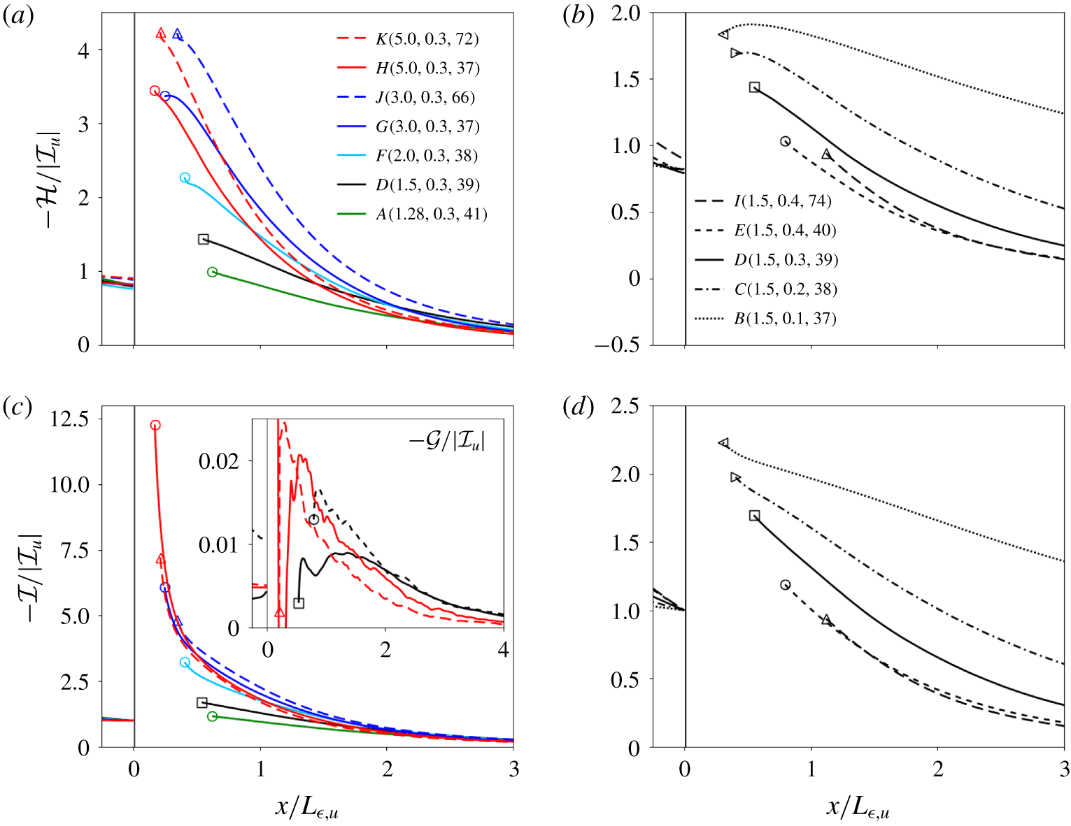
In figure 8 we compare the contribution of  ${\mathcal{G}}$, ${\mathcal{H}}$ and ${\mathcal{I}}$ for all simulated cases. Each profile is normalized with the preshock magnitude of the molecular diffusion term, $|{\mathcal{I}}_{u}|$. The velocity-scalar interaction term has a net positive contribution (i.e. amplification of dissipation, hence leading to better mixing), whereas the molecular diffusion term has a net negative contribution to the right-hand side equation (3.2), contributing to the ‘production’ and ‘destruction’ of scalar dissipation, respectively.
Whereas the velocity-scalar-gradient,  ${\mathcal{H}}$, and molecular diffusion, ${\mathcal{I}}$, terms are of the same order, the latter is always the largest in magnitude, for all cases and streamwise locations. The molecular diffusion term shows an effective jump in magnitude across the shock that is monotonically increasing with larger $M$, and smaller $M_{t}$. The effects of $Re_{\unicode[STIX]{x1D706}}$ are less obvious. The streamwise profiles show a monotonic shallowing of the slope downstream of the shock. In contrast, the velocity-scalar-gradient interaction term experiences a jump of magnitude across the shock that appears to saturate for $M\gtrapprox 3$ and increases with larger $Re_{\unicode[STIX]{x1D706}}$ and smaller $M_{t}$, in the wrinkled-shock regime. The contribution from the fluctuating-velocity/dissipation-gradient correlation term, ${\mathcal{G}}$, is predominantly positive, but much smaller (below 1 %) than the other two terms. The term ${\mathcal{G}}$ is only shown for selected cases in the inset, for clarity.
3.7 Spectra and PDFs
Spectra of (a) passive scalar and (b) scalar variance for different simulation cases at preshock and postshock locations. Each spectrum is normalized by its integral over all wavenumbers. Spectra for cases with higher  $Re_{\unicode[STIX]{x1D706}}$ ( ${\approx}70$) have been shifted up two decades. Postshock spectra are shifted by a factor of 3 relative to preshock counterparts. The black straight segment with $-5/3$ slope marks the extent of the inertial range of scales for the higher $Re_{\unicode[STIX]{x1D706}}$ cases, obtained from spectra of the kinetic energy (not shown).
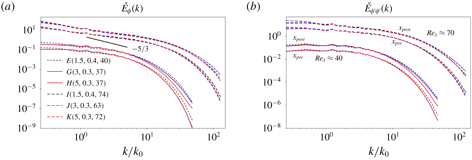
Time-averaged spectra of passive scalar calculated on transverse planes,  ${\check{E}}_{\unicode[STIX]{x1D719}}$, at preshock and postshock locations are compared in figure 9(a) for different simulation cases. Within the limited inertial range of length scales of the present simulations, the spectra of kinetic energy (not shown) upstream of the shock exhibit an approximate ${\check{E}}(k)\propto \unicode[STIX]{x1D716}^{2/3}k^{-5/3}$ scaling, consistent with the prediction of Kolmogorov (Reference Kolmogorov1941) for incompressible HIT. However, the passive scalar spectra in the inertial-convective range depart from the ${\check{E}}_{\unicode[STIX]{x1D712}}(k)\propto \unicode[STIX]{x1D716}^{-1/3}\unicode[STIX]{x1D712}k^{-5/3}$ prediction of Obukhov (Reference Obukhov1949) and Corrsin (Reference Corrsin1951) for passive scalar mixing in incompressible HIT. A slope shallower than $-5/3$ is observed in the inertial-convective range upstream of the shock for all cases, which may be attributed to the moderate Reynolds numbers of our simulations, following Danaila & Antonia (Reference Danaila and Antonia2009). For all cases, the spectral content of passive scalar and its variance increases across the shock for small scales (figure 9a,b), plausibly a consequence of the immediate amplification of transverse vorticity.
Comparison of time-averaged spectra of scalar dissipation on transverse planes for different simulation cases in the (a) preshock and (b) postshock states. Each spectrum is normalized to unitary integral. Spectra for cases with higher  $Re_{\unicode[STIX]{x1D706}}$ ( ${\approx}70$) are shifted up one decade for clarity. (c) Comparison of spectra of scalar dissipation at different streamwise locations for case $K$, where each spectrum in (c) is normalized by the value at the same wavenumber in the preshock spectrum.
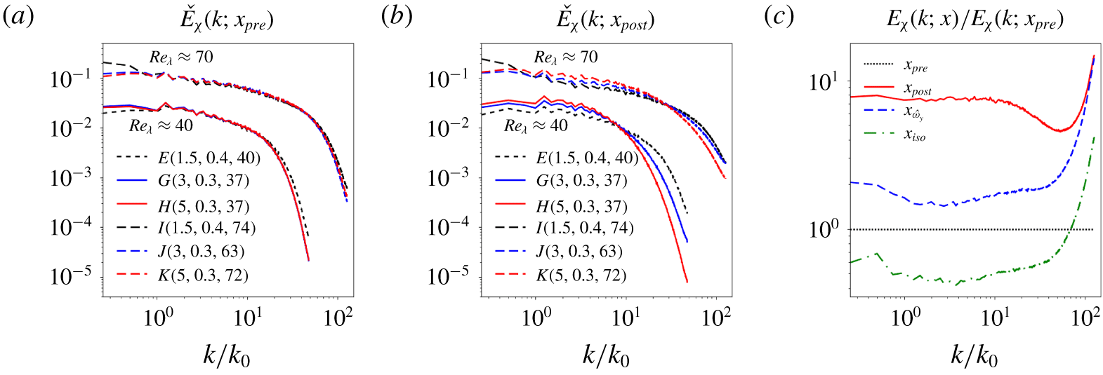
In contrast, spectra of scalar dissipation,  ${\check{E}}_{\unicode[STIX]{x1D712}}$, display a shift of spectral content across the shock from smaller to larger scales for increasing $M$ and lower $Re_{\unicode[STIX]{x1D706}}$ (see figure 10a,b). Taking case $K$ as an example (figure 10c), amplification of all wavenumbers is first observed in the postshock state ( $x_{post}$), predominantly at very small scales, followed by large and intermediate scales. Between $x_{post}$ and $x_{\hat{\unicode[STIX]{x1D714}}_{x}}$, the readjustment of transverse into streamwise vorticity counteracts the postshock viscous decay at small scales, such that the spectral content of scalar dissipation is reduced much more significantly at large and intermediate scales than at small scales. Downstream of $x_{\hat{\unicode[STIX]{x1D714}}_{x}}$, viscous decay affects all scales similarly, preserving the shape of the spectra.
Time-averaged, transverse-plane probability density functions (PDFs) of passive scalar, its variance and its dissipation for case  $K$ at different streamwise locations are shown in figure 11. Super-Gaussian passive scalar PDFs, indicative of intermittency, show a monotonic narrowing downstream as the scalar variance decreases, as previously observed in Tian et al. (Reference Tian, Jaberi, Li and Livescu2017) and Boukharfane et al. (Reference Boukharfane, Bouali and Mura2018). The streamwise evolution of PDFs of scalar variance and scalar dissipation (figure 11b,c) was not reported in those previous studies. PDFs of scalar dissipation shift significantly across the shock toward larger values, followed downstream by a progressive recovery to preshock shapes, completed between the streamwise locations of maximum enstrophy ( $x_{\hat{\unicode[STIX]{x1D714}}_{x}}$) and small-scale isotropy recovery ( $x_{iso}$). Similar observations hold for other cases (not shown), with higher $Re_{\unicode[STIX]{x1D706}}$ resulting in wider tails of scalar dissipation, consistent with the study of passive scalar mixing in compressible HIT by Ni (Reference Ni2015).
Probability density functions of (a) passive scalar, (b) scalar variance and (c) scalar dissipation for case  $K$ at $x_{pre}$ (dotted), $x_{post}$ (solid), $x_{\hat{\unicode[STIX]{x1D714}}_{x}}$ (dashed), $x_{iso}$ (dash–dotted). The dash–dot–dotted line in (a) corresponds to a Gaussian distribution with zero mean and the standard deviation of the PDF of passive scalar at $x_{iso}$.

4 Flow topology and conditioned dissipation rate
4.1 Characterization of local flow topology
Deformation, rotation and stretching (hence mixing) of material elements is characterized by local flow topologies that relate streamline patterns moving with the fluid element to the invariants of the velocity gradient tensor by means of critical point theory (Chong, Perry & Cantwell Reference Chong, Perry and Cantwell1990). Compared with incompressible flows, compressibility introduces a richer set of topologies and different formulations of the topology analysis (Pirozzoli & Grasso Reference Pirozzoli and Grasso2004; Suman & Girimaji Reference Suman and Girimaji2010; Vaghefi & Madnia Reference Vaghefi and Madnia2015; Parashar, Sinha & Srinivasan Reference Parashar, Sinha and Srinivasan2019). In the present study, following Suman & Girimaji (Reference Suman and Girimaji2010), we normalize the velocity gradient tensor  $\unicode[STIX]{x1D608}_{ij}=\unicode[STIX]{x2202}_{i}u_{j}$ as $\unicode[STIX]{x1D622}_{ij}=\unicode[STIX]{x1D608}_{ij}/\sqrt{\unicode[STIX]{x1D608}_{pq}\unicode[STIX]{x1D608}_{pq}}$, from which normalized strain-rate and rotation-rate tensors are obtained as $\unicode[STIX]{x1D634}_{ij}=(\unicode[STIX]{x1D622}_{ij}+\unicode[STIX]{x1D622}_{ji})/2$ and $\unicode[STIX]{x1D638}_{ij}=(\unicode[STIX]{x1D622}_{ij}-\unicode[STIX]{x1D622}_{ji})/2$, respectively. The three invariants of $\unicode[STIX]{x1D622}_{ij}$ are then expressed as $p=-\text{tr}(\unicode[STIX]{x1D622}_{ij})$, $q=\frac{1}{2}(p^{2}-\unicode[STIX]{x1D634}_{ij}\unicode[STIX]{x1D634}_{ji}-\unicode[STIX]{x1D638}_{ij}\unicode[STIX]{x1D638}_{ji})$ and $r=-\det (\unicode[STIX]{x1D622}_{ij})$, and determine the character (real or complex) of the three eigenvalues of $\unicode[STIX]{x1D608}_{ij}$, thus defining the local streamline pattern and flow topology. The $pqr$ space is partitioned into ten different flow topologies (see figure 12) by the $r=0$ plane and three dividing surfaces, $S1(a,b)$, defined by $(p/3)(q-2p^{2}/9)\mp (2/27)\sqrt{-3q+p^{2}}-r=0$, and $S2$, defined by $pq=r$. Surfaces $S1(a,b)$ separate regions with three real eigenvalues (non-focal topologies) from regions with one real and two complex conjugate eigenvalues (focal topologies). Surface $S2$ contains purely imaginary eigenvalues. Stable (unstable) topologies indicate that the local streamlines are directed toward (away from) the critical point.
Flow topologies in  $pqr$ space mapped onto three representative planes with (a) $p<0$ (extension), (b) $p=0$ (volume-preserving) and (c) $p>0$ (contraction), partitioned by the intersections of each plane with the dividing surfaces $S1a$ (dashed), $S1b$ (dash–dotted), $S2$ (solid) and the $r=0$ plane (dotted): SFS, stable focus stretching; UFS, unstable focus stretching; SFC, stable focus compressing; UFC, unstable focus compressing; SNSS, stable-node/saddle/saddle; UNSS, unstable-node/saddle/saddle; SN3, stable node/stable-node/stable-node; UN3, unstable-node/unstable-node/unstable-node; SSN3, stable-star-node/stable-star-node/stable-star-node; USN3, unstable-star-node/unstable-star-node/unstable-star-node. The last two topologies correspond to the intersection of $S1a$ and $S1b$ for $p<0$ and $p>0$, respectively.

Probability density functions of  $p$ (a–c), $q$ (d–f) and $r$ (g–i), along with normalized distributions of scalar dissipation conditioned on the respective invariant, extracted at $x_{pre}$ (a,d,g), $x_{post}$ (b,e,h) and $x_{iso}$ (c,f,i) for cases with different $(M,M_{t},Re_{\unicode[STIX]{x1D706}})$. Each plot shows the PDFs of the invariant on the bottom curves (left vertical axis), and the conditioned scalar dissipation distributions, $\hat{E}(\unicode[STIX]{x1D712}|f)$ for $f\in (p,q,r)$, on top (right vertical axis).

4.2 One-dimensional PDFs and conditioned scalar dissipation distributions
For each case and streamwise location,  $E(\unicode[STIX]{x1D712}|f)$ denotes the distribution of scalar dissipation, $\unicode[STIX]{x1D712}$, conditioned on the invariant $f\in (p,q,r)$. This distribution is subsequently time-averaged and normalized by the Reynolds-averaged scalar dissipation, $\overline{\unicode[STIX]{x1D712}}$, at the same streamwise location, to obtain $\hat{E}(\unicode[STIX]{x1D712}|f)=\langle E(\unicode[STIX]{x1D712}|f)\rangle /\overline{\unicode[STIX]{x1D712}}$, where $\langle \cdot \rangle$ is the time-averaging operator. In figure 13 we show time-averaged PDFs of the $p$,
$p$,  $q$ and $r$ invariants, and the corresponding normalized conditional distributions of scalar dissipation, $\hat{E}(\unicode[STIX]{x1D712}|p)$, $\hat{E}(\unicode[STIX]{x1D712}|q)$ and $\hat{E}(\unicode[STIX]{x1D712}|r)$, extracted at the $x_{pre}$ (preshock), $x_{post}$ (postshock) and $x_{iso}$ (return to vorticity-variance isotropy) locations defined in § 3.1. Results from only a subset of the simulation cases are plotted for clarity, to highlight the effect of $M$,
$M$,  $M_{t}$ and $Re_{\unicode[STIX]{x1D706}}$.
Probability density functions of  $p$ (figure 13a–c) are nearly symmetric about $p=0$ (i.e. incompressible events), where they peak, wider for larger $M_{t}$ (owing to the larger velocity fluctuations relative to the sound speed), and narrower for increasing $M$ and $Re_{\unicode[STIX]{x1D706}}$. At $x_{post}$ the peak of the $p$-PDF is nearly half of its preshock magnitude. Normalized distributions of scalar dissipation conditioned on $p$,
$p$,  $\hat{E}(\unicode[STIX]{x1D712}|p)$, also peak at $p=0$, but are significantly flattened at $x_{post}$, as the $p$-PDFs widen, indicating a more even distribution of the dissipation across compressible flow topologies compared to the preshock state. The broken-shock regime simulation shows the largest asymmetry of $\hat{E}(\unicode[STIX]{x1D712}|p)$ at $x_{pre}$ and $x_{post}$. By $x_{iso}$ all distributions have widened relative to $x_{pre}$ and become nearly symmetric.
Preshock  $q$-PDFs (figure 13d–f) are negatively skewed (i.e. strain-rate dominated), more so for increasing $Re_{\unicode[STIX]{x1D706}}$. The shape of the $q$-PDFs is altered at $x_{post}$, especially for larger $M$, increasing the magnitude of the peak (found at $q\approx 0$), which narrows the core of the distributions. At $x_{iso}$, the $q$-PDFs recover the preshock shape, nearly overlapping for all cases considered. The normalized distributions of scalar dissipation conditioned on $q$,
$q$,  $\hat{E}(\unicode[STIX]{x1D712}|q)$, are skewed toward $q<0$, indicating that scalar dissipation occurs predominantly in strain-dominated topologies. At $x_{pre}$ and $x_{iso}$ the distributions nearly collapse for all simulations. However, at $x_{post}$, larger $M$ tends to reduce the skewness, and a local maximum at $q\approx 0$ develops. Increasing $Re_{\unicode[STIX]{x1D706}}$ counteracts the effects of a larger $M$ on both the $\text{PDF}(q)$ and $\hat{E}(\unicode[STIX]{x1D712}|q)$ at $x_{post}$.
Probability density functions of  $r$ (figure 13g–i) at $x_{pre}$ and $x_{iso}$ are nearly insensitive to $M$,
$M$,  $M_{t}$ and $Re_{\unicode[STIX]{x1D706}}$, and appear skewed toward positive values, corresponding to predominantly unstable topologies (flow directed away from critical points, whether rotating or strained), and indicative of the dissipative nature of DHIT. At $x_{post}$, higher $M$ and smaller $Re_{\unicode[STIX]{x1D706}}$ narrow and symmetrize the PDFs, which attain larger peaks at $r=0$. A tendency toward symmetrization of the PDF of this third invariant was observed using LIA and DNS by Ryu & Livescu (Reference Ryu and Livescu2014). The invariant $r$ represents the competition between the production of kinetic energy dissipation ( $r>0$) and enstrophy ( $r<0$) (see Vaghefi & Madnia Reference Vaghefi and Madnia2015; Yu & Lu Reference Yu and Lu2019). Thus, the symmetrization of the $r$-PDF indicates a relative increase of enstrophy production across the shock, and translates farther downstream into a larger scalar dissipation at small scales (as seen in figure 10c)). The distribution of $\unicode[STIX]{x1D712}$ conditioned on $r$,
$r$,  $\hat{E}(\unicode[STIX]{x1D712}|r)$, is largely skewed toward $r>0$ (where production of TKE dissipation prevails) at all streamwise locations, more so for larger $Re_{\unicode[STIX]{x1D706}}$, peaking at $r\approx 0.1$ for $x_{pre}$ and $x_{iso}$, while flattening and bringing its peak closer to $r=0$ at $x_{post}$.
4.3 Joint  $qr$-PDFs and conditioned scalar dissipation distributions

Joint  $qr$-PDFs (dashed black-white contour lines at 15 % and 60 % of the peak value per plot) and conditioned $\unicode[STIX]{x1D712}$ distributions (jet-scale contours masked below 1 % of the peak of the $qr$-PDF) for case $K$ at different streamwise locations (left to right: $x_{pre}$, $x_{post}$, $x_{\hat{\unicode[STIX]{x1D714}}_{x}}$, $x_{iso}$) and values of $p$ (top to bottom: $3/2$, 0 and $-3/2$ times the standard deviation, $\unicode[STIX]{x1D70E}_{p}$, per streamwise location). Short-dashed black lines: $S1a$, $S1b$, $S2$ curves and $q$-axis. Colour map represents the conditioned scalar dissipation (blue to green to yellow to red, from zero to the highest value in each figure).

Distinct regions in the  $qr$ planes for different values of $p$ define a variety of flow topologies (figure 12). In figure 14 we show, for case $K$
$K$  $(M,M_{t},Re_{\unicode[STIX]{x1D706}}=5,0.3,72)$, joint $qr$-PDFs (contour lines) and conditional $\unicode[STIX]{x1D712}$-distributions (coloured contour map) at $x_{pre}$, $x_{post}$and $x_{iso}$for three values of $p$: negative (extension), zero (incompressible) and positive (contraction). The teardrop shape commonly found in incompressible flows is recovered for $p=0$ at the three locations. It is observed that $\unicode[STIX]{x1D712}$ concentrates on the right lower tail ( $q<0$ and $r>0$) of the teardrop, below and near the $S1b$ line, which confirms UNSS as the most dissipative topology at those locations, consistent with previous findings for compressible and incompressible turbulence (Brethouwer, Hunt & Nieuwstadt Reference Brethouwer, Hunt and Nieuwstadt2003; Danish et al. Reference Danish, Suman and Girimaji2016). Non-zero $p$ values modify the shape of the $qr$-PDFs, symmetrizing its outer edge, whereas $\unicode[STIX]{x1D712}$ remains largely concentrated in the UNSS topology. In figure 15 we compare joint $qr$-PDF and conditioned $\unicode[STIX]{x1D712}$ distributions for $p=0$ among the three cases with the higher $Re_{\unicode[STIX]{x1D706}}$ ( ${\approx}70$). As $M$ increases, the $qr$-PDF preserves the teardrop shape but considerably narrows toward the origin. Conditional $\unicode[STIX]{x1D712}$ distributions still appear predominantly concentrated in the fourth quadrant for larger $M$, with the peak moving toward the origin.
Joint  $qr$-PDFs (dashed black-white contour lines at 15 % and 60 % of the peak value per plot) and conditioned $\unicode[STIX]{x1D712}$ distributions (jet-scale contours masked below 1 % of the peak of the $qr$-PDF) for case $I$ (a), $J$ (b), $K$ (c) at $x_{post}$ for $p=0$. Colour map represents the conditioned scalar dissipation (blue to green to yellow to red, from zero to highest value in each plot).
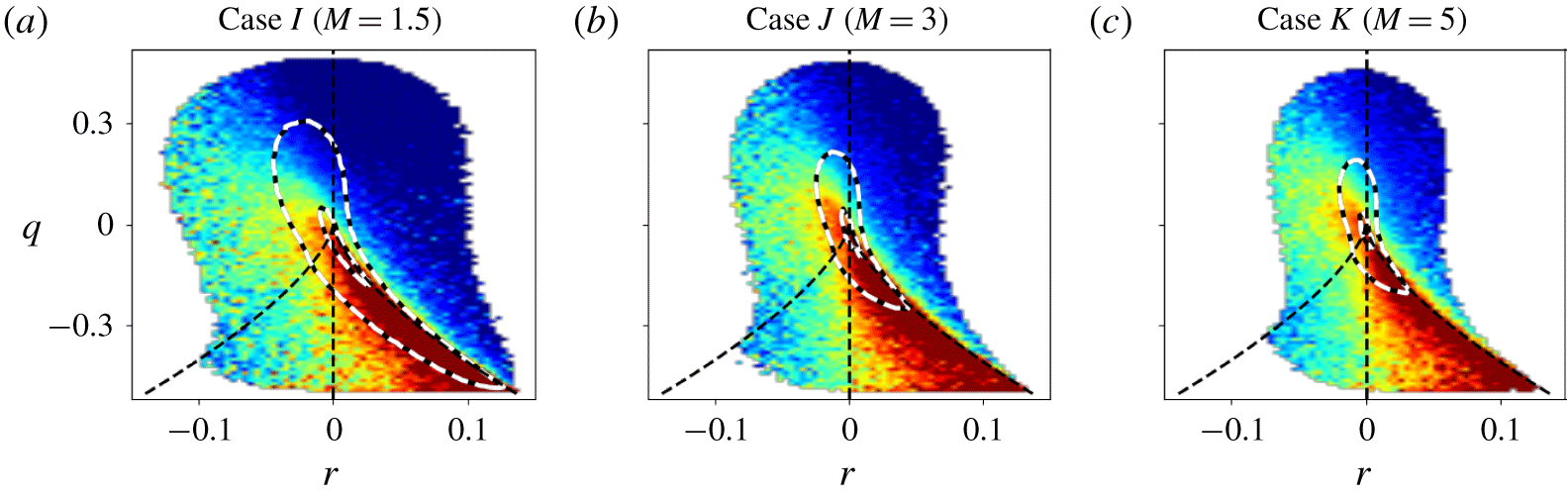
4.4 Proportion of topologies and their contribution to the scalar dissipation
Streamwise evolution of the time-averaged proportion of (a) flow topologies,  $\langle {\mathcal{T}}_{p}\rangle$, and (b) the scalar dissipation in each topology, $\langle \unicode[STIX]{x1D712}_{p\mid {\mathcal{T}}}\rangle$, for different simulations. Topologies ordered by largest relative contribution (top to bottom). Unsteady shock regions are removed and streamwise axes are normalized by the dissipation length scale immediately upstream of the shock. Symbols mark the postshock location, $x_{post}$.

In figure 16(a) we compare, for different simulation cases, the streamwise evolution of the time-averaged proportion of grid cells with a given flow topology,  $\langle {\mathcal{T}}_{p}(x)\rangle$. The corresponding time-averaged proportion of scalar dissipation rate carried by each topology at each streamwise location, denoted by $\langle \unicode[STIX]{x1D712}_{p\mid {\mathcal{T}}}(x)\rangle$, is shown in Figure 16(b). For all simulation cases, stable focus stretching (SFS) is the most dominant topology, accounting for over one third of the volume, followed by unstable-node/saddle/saddle (UNSS) ( ${\approx}25\,\%$), unstable focus compressing (UFC) ( ${\approx}20\,\%$), stable-node/saddle/saddle (SNSS) ( ${\approx}10\,\%$), stable focus compressing (SFC) ( ${\approx}8\,\%$) and unstable focus stretching (UFS) ( ${\approx}1\,\%$). The SFS topology is reflective of rotating streamlines around a critical point, characteristic of vortical motions predominant in turbulence. In contrast, the bi-axial stretching imposed by the UNSS topology results in the largest contribution to the dissipation. Regions of high kinetic energy dissipation of the background flow are linked to the stretching and dissipation of the scalar variance, hence explaining the largest contribution of UNSS to the overall scalar dissipation.
Downstream of the unsteady shock region, the proportions of SFS and UNSS decrease, whereas those of UFS and SNSS increase by comparable amounts, respectively. These changes are amplified with larger  $M$. Increasing $Re_{\unicode[STIX]{x1D706}}$ enhances the proportion of non-focal topologies (UNSS and SNSS), reducing all others. The reduction of the fraction of $p=0$ events across the shock (figure 13b) results in a decreased proportion of focal topologies (not shown), consistent with observations by Vaghefi & Madnia (Reference Vaghefi and Madnia2015) on the proportion of flow topologies conditioned on $p$ in compressible mixing layers. The SNSS topology includes one direction of extension and two of contraction (opposite to UNSS), whereas UFS occurs for $p<0$ (extension). Compression increases the probability of stable, non-focal topologies, particularly SNSS (Suman & Girimaji Reference Suman and Girimaji2010; Wang et al. Reference Wang, Shi, Wang, Xiao, He and Chen2012; Vaghefi & Madnia Reference Vaghefi and Madnia2015). This is justified by the convergence of local streamlines toward critical points experienced when the volume of fluid element decreases. The SFS topology is inhibited in regions of large compression, consistent with the postshock decrease observed in our simulations.
Dominance of SFS and UNSS topologies was previously observed in compressible HIT (e.g. Suman & Girimaji Reference Suman and Girimaji2010; Wang et al. Reference Wang, Shi, Wang, Xiao, He and Chen2012) and STI (Ryu & Livescu Reference Ryu and Livescu2014; Boukharfane et al. Reference Boukharfane, Bouali and Mura2018), the latter for lower  $M$,
$M$,  $M_{t}$ and $Re_{\unicode[STIX]{x1D706}}$ than the ones considered here. The downstream evolution of these topologies has not been reported to date.
An initial recovery of the proportion of each topology toward its preshock state follows shortly downstream of the shock, within the region of acoustic-to-vortical energy transfer (see figure 2a,b). Increasing  $Re_{\unicode[STIX]{x1D706}}$ shortens this initial recovery distance. Farther downstream, cases with lower $M$ recover the upstream proportion for each topology within $3L_{\unicode[STIX]{x1D716},u}$, whereas cases with larger $M$ show a sustained downstream reduction of SFS and UNSS topologies at the expense of an increased proportion of SFC and UFC topologies. The order of dominant topologies remains practically unchanged within the computational domain for all simulations. The UNSS and SFS topologies are the most sensitive to changes of dilatation (Parashar et al. Reference Parashar, Sinha and Srinivasan2019), which is consistent with the larger changes experienced by these topologies across the shock (figure 16a).
From figure 16(b), UNSS presents the largest proportion of scalar dissipation ( ${\approx}40\,\%$), followed by SFS ( ${\approx}33\,\%$), swapping order with respect to the dominant topology proportions, ${\mathcal{T}}_{p}$, discussed earlier, while all other topologies maintain the same order. Results (not shown) for the ratio $\langle \unicode[STIX]{x1D712}_{p\mid {\mathcal{T}}}\rangle /{\mathcal{T}}_{p}$, indicate that UNSS, followed by SNSS and then SFS, have the largest relative mean scalar dissipation when conditioned on the topology. Thus, nonfocal topologies are more dissipative than focal topologies, as also found for the kinetic energy dissipation in compressible mixing layers (Vaghefi & Madnia Reference Vaghefi and Madnia2015). Multiscale analyses of compressible HIT have shown that UNSS is favoured at small scales (Danish & Meneveau Reference Danish and Meneveau2018). The larger amplification of small scales seen across the shock, combined with the dominance of UNSS as the most dissipative topology can help explain the postshock increase of scalar dissipation.
Among focal topologies, those that are fully compressing (SFC) or fully stretching (UFS) are less dissipative than those with simultaneous compressing and stretching (SFS and UFC). These results remain valid downstream of the unsteady shock region and are consistent with findings in compressible HIT (Danish et al. Reference Danish, Suman and Girimaji2016). Besides, UNSS and SFS are known to present the maximum vortex stretching rate on average from studies of mixing layers (Vaghefi & Madnia Reference Vaghefi and Madnia2015). Although associated with weaker enstrophy content, UNSS regions present high vorticity stretching rates, explaining their predominant dissipation of TKE and scalar variance. Despite the contraction of vorticity that dominates regions of compression, SFS (characterized by radial contraction and axial stretching), presents a net positive stretching rate of vorticity and thus contributes to the dissipation of TKE and scalar variance. The tendency of vortex tubes (associated mainly with SFS topologies) to orient parallel to the shock downstream could then be linked to the increase of dissipation (of TKE and scalar variance). Studies tracking vortex tubes across the shock would help elucidate this issue.
However, immediately downstream of the unsteady shock region, UNSS and SFS topologies reduce their relative contribution to the scalar dissipation, whereas all other topologies increase theirs. Larger  $M$ amplifies these effects for all topologies except for SFS. At all streamwise locations, larger $Re_{\unicode[STIX]{x1D706}}$ shifts the contribution of UNSS and SNSS towards a larger proportion of the scalar dissipation, reducing the relative contribution of all other topologies, consistent with the effects on ${\mathcal{T}}_{p}$ seen earlier. Likewise, $\langle \unicode[STIX]{x1D712}_{p\mid {\mathcal{T}}}\rangle$ profiles also show an initial recovery shortly downstream of the shock, followed by a slower asymptotic evolution toward preshock values, except for a sustained decrease of scalar dissipation proportion seen for SFS at the expense of an increase for UFS.
To investigate dominant paths of transition between different topologies, Lagrangian tracking of 10 000 fluid particles seeded upstream of the shock is conducted for case  $D$ (
$D$ ( $M,M_{t},Re_{\unicode[STIX]{x1D706}}\approx 1.5,0.3,40$), following their trajectories across and downstream of the shock. The time origin of each trajectory is shifted to match its shock-crossing instant. From the ensemble of trajectories, the probability of transition from each flow topology into every possible topology is calculated, as a function of non-dimensional time. From this study, it is concluded that before and after the unsteady shock region, each topology has a high probability of not changing its topology. The SFS and UNSS topologies are the least prone to change, particularly upstream of the shock, whereas UFS, SNSS and SFC are most likely to transition, although still with small probability. Across the shock, most topologies (SFS, UNSS, UFC, SFC) exhibit a high probability of transitioning into SNSS. This is most noticeable for SFS and UNSS, which are the most dominant topologies in the flow, and also with the largest contributions to the passive scalar dissipation. Although SNSS shows the largest probability of not changing across the shock, transitions into SFS and UNSS are frequent, and remain significant farther downstream.
In summary, preshock flow topologies and their contribution to the scalar dissipation are altered across the shock. The widening of the nearly symmetric PDF of dilatation across the shock enhances the role of compressible flow topologies (compression-only, SFC, and expansion-only, UFS) on the scalar dissipation, at the expense of a decreased contribution from those topologies that are dominant in incompressible flows (SFS and UNSS). Despite the symmetry of the PDFs of dilatation (figure 13), preshock fractions of SFC and UFS topologies are asymmetric, favouring the compression-only SFC pattern. Immediately downstream of the shock, the widened (still symmetric) PDFs of dilatation enhance the importance of the expansion-only UFS topology. The UFC (involving radial stretching and axial contraction with outward spiraling streamlines) and SNSS (bi-axial contraction) topologies are also favoured and increase their contribution to scalar dissipation across the shock. The observed changes become more significant for stronger shocks (larger  $M$).
$M$).
5 Alignment of scalar gradient, vorticity, shock normal and strain
Preferential alignment of vorticity and scalar gradient with the strain-rate eigenvectors plays a key role in the dissipation of turbulence kinetic energy and passive scalar variance (Kerr Reference Kerr1985; Ashurst et al. Reference Ashurst, Kerstein, Kerr and Gibson1987), and forms the basis of some structure-based models of turbulence and passive scalar fine scales (Misra & Pullin Reference Misra and Pullin1997; Pullin Reference Pullin2000). Amplification of passive scalar dissipation brought by the net positiveness of the term  ${\mathcal{H}}=\overline{\unicode[STIX]{x1D735}\unicode[STIX]{x1D719}\boldsymbol{\cdot }\boldsymbol{A}\boldsymbol{\cdot }\unicode[STIX]{x1D735}\unicode[STIX]{x1D719}}$ in the transport equation for $\overline{\unicode[STIX]{x1D712}}$ (see § 3.6) is related to the alignment of the principal strain directions and the scalar gradient. In this section we present parametric studies of the change of alignments across the unsteady shock region conditioned on flow topology. This is followed by a global assessment of the relation between these alignments and their contribution to the dissipation of passive scalar fluctuations. We denote the eigenvectors of the strain-rate tensor, $\unicode[STIX]{x1D61A}_{ij}=(\unicode[STIX]{x1D608}_{ij}+\unicode[STIX]{x1D608}_{ji})/2$, as $\unicode[STIX]{x1D736}$, $\unicode[STIX]{x1D737}$ and $\unicode[STIX]{x1D738}$, with their respective eigenvalues ordered from most extensional to most compressive, $\unicode[STIX]{x1D6FC}\geqslant \unicode[STIX]{x1D6FD}\geqslant \unicode[STIX]{x1D6FE}$.
5.1 Alignments conditioned on flow topology across the shock
In figure 17 we show the change across the unsteady shock region of alignments between the scalar gradient,  $\unicode[STIX]{x1D735}\unicode[STIX]{x1D719}$, and both the most extensive, $\unicode[STIX]{x1D736}$, and the most compressive, $\unicode[STIX]{x1D738}$, principal strain directions, by means of time-averaged PDFs of the cosine of the angles between those directions at preshock and postshock streamwise locations. Preferential alignment with $\unicode[STIX]{x1D738}$ is seen for all topologies, ordered left-to-right from most-to-least aligned with $\unicode[STIX]{x1D738}$ ( $\text{UNSS}>\text{SNSS}>\text{SFS}>\text{UFC}>\text{UFS}>\text{SFC}$). The preshock state of alignments is practically insensitive to $M$,
$M$,  $M_{t}$ and $Re_{\unicode[STIX]{x1D706}}$, consistent with Lee, Girimaji & Kerimo (Reference Lee, Girimaji and Kerimo2009). Thus, for clarity, only case $E$ is shown at the preshock location, $x_{pre}$. The UNSS topology presents the most preferred alignment of $\unicode[STIX]{x1D735}\unicode[STIX]{x1D719}$ and $\unicode[STIX]{x1D738}$, followed by SNSS and SFS, whereas SFC shows the least alignment (although still dominant) between those two directions, in favour of an increased alignment of $\unicode[STIX]{x1D735}\unicode[STIX]{x1D719}$ with $\unicode[STIX]{x1D736}$. Two of the topologies with better alignment of $\unicode[STIX]{x1D735}\unicode[STIX]{x1D719}$ and $\unicode[STIX]{x1D738}$ at $x_{pre}$, UNSS and SFS, were found in § 4.4 to have the largest contribution to the scalar dissipation. These preshock results are consistent with the findings for compressible DHIT in Danish et al. (Reference Danish, Suman and Girimaji2016), who attributed variations in the amplification (production) of scalar dissipation to the ability of a topology to enhance the alignment between the scalar gradient and the most compressive strain-rate eigendirection.
Probability density functions of the cosine of the angle ( $\unicode[STIX]{x1D701}$) between the passive scalar gradient, $\unicode[STIX]{x1D735}\unicode[STIX]{x1D719}$, and (a) the most extensional, $\unicode[STIX]{x1D736}$, and (b) the most compressive, $\unicode[STIX]{x1D738}$, eigenvectors of the strain-rate tensor, conditioned on topology for different simulation cases, comparing preshock and postshock states. In the preshock state, case $E$ (green dotted lines) is representative of all other cases (not shown for clarity).
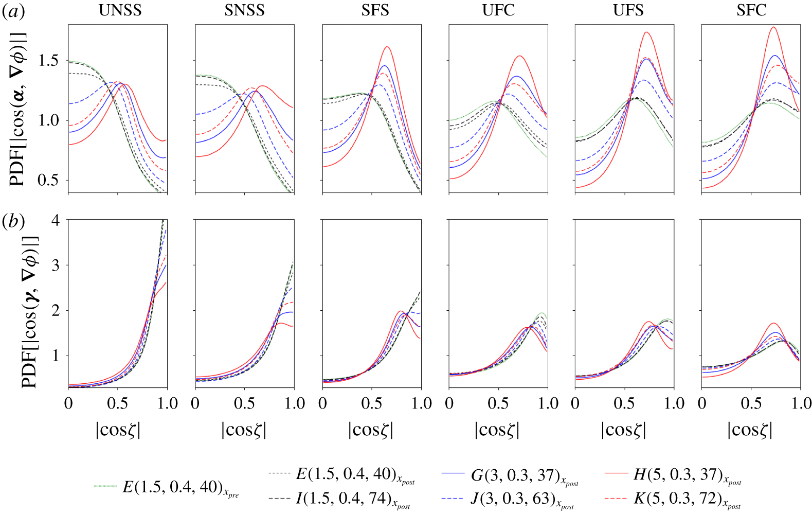
However, at  $x_{post}$ the alignments depend strongly on $M$ and $Re_{\unicode[STIX]{x1D706}}$, but not on $M_{t}$. Alignment with $\unicode[STIX]{x1D738}$ becomes less dominant for all topologies, favouring better alignment with $\unicode[STIX]{x1D736}$. This trend is stronger with larger $M$ and smaller $Re_{\unicode[STIX]{x1D706}}$. Cases in the broken-shock regime ( $A$, not shown, $E$ and $I$) result in much smaller changes of alignments than wrinkled-shock cases, likely from the wider unsteady shock region of broken shocks.
In figure 18 we show changes, across the shock region, of alignments between  $\unicode[STIX]{x1D735}\unicode[STIX]{x1D719}$ and the intermediate strain-rate eigenvector ( $\unicode[STIX]{x1D737}$), the vorticity ( $\unicode[STIX]{x1D74E}$) and the mean shock-normal direction ( $x$). All topologies present nearly identical preshock and postshock PDFs, so only SFS, the most dominant topology found in § 4, will be discussed. Preshock alignment between $\unicode[STIX]{x1D735}\unicode[STIX]{x1D719}$ and $\unicode[STIX]{x1D737}$ is small, further decreasing at $x_{post}$, in favour of better alignment with $\unicode[STIX]{x1D736}$. Larger $M$ and smaller $Re_{\unicode[STIX]{x1D706}}$ significantly reduce the alignment of $\unicode[STIX]{x1D735}\unicode[STIX]{x1D719}$ with $\unicode[STIX]{x1D737}$ at $x_{post}$, while $M_{t}$ has a negligible effect. Upstream of the shock, the passive scalar gradient is predominantly orthogonal to the vorticity, consistent with previous studies for incompressible and compressible HIT and STI (Kerr Reference Kerr1985; Ashurst et al. Reference Ashurst, Kerstein, Kerr and Gibson1987; Boukharfane et al. Reference Boukharfane, Bouali and Mura2018). As expected, no preferential alignment exists between $\unicode[STIX]{x1D735}\unicode[STIX]{x1D719}$ and $x$ in the preshock state. At $x_{post}$, the scalar gradient becomes slightly more orthogonal to $\unicode[STIX]{x1D74E}$ and significantly aligned with $x$, more so for increasing $M$ and decreasing $Re_{\unicode[STIX]{x1D706}}$. A similar trend with $M$ was also observed by Boukharfane et al. (Reference Boukharfane, Bouali and Mura2018), who, however, did not explore $Re_{\unicode[STIX]{x1D706}}$ effects nor condition the alignments on topologies, presently analysed.
Probability density functions of the cosine of the angle between the scalar gradient,  $\unicode[STIX]{x1D735}\unicode[STIX]{x1D719}$, and (a) the intermediate eigenvector, $\unicode[STIX]{x1D737}$, of the velocity gradient tensor, (b) the vorticity, $\unicode[STIX]{x1D74E}$, and (c) the streamwise axis, $x$, conditioned on the SFS topology (similar PDFs of these quantities are observed for all other topologies).

5.2 Barycentric map representation of alignments
We propose a combined representation of the alignments between a vector of interest,  $\boldsymbol{v}$, (e.g. vorticity, scalar gradient) and the three strain-rate eigenvectors ( $\unicode[STIX]{x1D736}$, $\unicode[STIX]{x1D737}$ and $\unicode[STIX]{x1D738}$) by the barycentric coordinates of a point inside an equilateral triangle, calculated from the cosines of the angles formed by the vector of interest, $\boldsymbol{v}$, and the strain-rate eigenvectors as $(a,b,c)=(\cos (\unicode[STIX]{x1D736},\boldsymbol{v}),\cos (\unicode[STIX]{x1D737},\boldsymbol{v}),\cos (\unicode[STIX]{x1D738},\boldsymbol{v}))/\unicode[STIX]{x1D70E}$, where $\unicode[STIX]{x1D70E}=\cos (\unicode[STIX]{x1D736},\boldsymbol{v})+\cos (\unicode[STIX]{x1D737},\boldsymbol{v})+\cos (\unicode[STIX]{x1D738},\boldsymbol{v})$, such that $a+b+c=1$. The corresponding Cartesian coordinates on the $\unicode[STIX]{x1D709}\unicode[STIX]{x1D702}$ plane of the triangle are $(\unicode[STIX]{x1D709},\unicode[STIX]{x1D702})=(b/2,\sqrt{3}b/2+c)$. The vertices of the triangle, with Cartesian coordinates given by $(0,0)$, $(1/2,\sqrt{3}/2)$ and $(1,0)$, represent perfect alignment with $\unicode[STIX]{x1D736}$, $\unicode[STIX]{x1D737}$ and $\unicode[STIX]{x1D738}$, respectively. At each streamwise location and for each $\boldsymbol{v}$ of interest, we calculate the $\unicode[STIX]{x1D709}\unicode[STIX]{x1D702}$-joint PDF of the alignments of $\boldsymbol{v}$ with $\unicode[STIX]{x1D736}$, $\unicode[STIX]{x1D737}$ and $\unicode[STIX]{x1D738}$ combined, along with the distribution of the passive scalar dissipation, $\unicode[STIX]{x1D712}$, conditioned on those alignments. Joint PDFs and conditioned distributions are then time-averaged, and can be represented by contours on the barycentric map.
In figure 19 we show, on the barycentric map, time-averaged joint PDFs of alignments between scalar gradient, vorticity and unit vector along  $x$ with the principal strain directions. As before, the preshock state is shown only for case $E$, representative of all other cases. All PDFs have a common, single-peaked shape, monotonically decreasing away from the peak and, thus, are suitable for representation by a reduced signature: the peak (marked by a symbol) and the isoline at 80 % of the peak value. The peak location together with the shape and spread of the 80 % isoline are used to compare PDFs and conditioned distributions for different simulation cases.
Barycentric map representation of the PDFs of alignment between the eigenvectors (most extensive,  $\unicode[STIX]{x1D736}$; intermediate, $\unicode[STIX]{x1D737}$; and most compressive, $\unicode[STIX]{x1D738}$) of the strain-rate tensor and (a) passive scalar gradient ( $\unicode[STIX]{x1D735}\unicode[STIX]{x1D719}$), (b) vorticity ( $\unicode[STIX]{x1D74E}$) and (c) the streamwise direction ( $x$). Symbols mark the peak of the PDF, whereas lines represent the isocontour at 80 % of the peak value of each distribution. Segments normal to each triangle side mark the $1/4$, $1/2$ and $3/4$ partition points. Insets zoom into the region of interest of each barycentric map.

In the preshock state,  $\unicode[STIX]{x1D735}\unicode[STIX]{x1D719}$ is preferentially aligned with $\unicode[STIX]{x1D738}$, followed by $\unicode[STIX]{x1D736}$ and, much less, with $\unicode[STIX]{x1D737}$ (figure 19a). At $x_{post}$, better alignment with $\unicode[STIX]{x1D736}$ is seen, at the expense of a reduced alignment with $\unicode[STIX]{x1D738}$ and $\unicode[STIX]{x1D737}$, increasing the orthogonality with the latter. Larger $M$ enhances this trend, bringing the peak of the postshock PDF closer to the $\unicode[STIX]{x1D6FC}\unicode[STIX]{x1D6FE}$ side of the triangle and narrowing the PDF. Increasing $Re_{\unicode[STIX]{x1D706}}$ counteracts the effect of larger $M$, widening the PDF and returning its peak toward its preshock state. These trends agree with the alignments of the scalar gradient conditioned on different flow topologies (§ 5.1).
Preferential alignment of vorticity with the intermediate strain eigenvector,  $\unicode[STIX]{x1D737}$ is clearly inferred from figure 19(b). The shape of the joint PDF along the $\unicode[STIX]{x1D6FC}\unicode[STIX]{x1D6FD}$ side of the triangle is indicative of the predominant orthogonality of $\unicode[STIX]{x1D74E}$ with the most compressive principal direction of strain, $\unicode[STIX]{x1D738}$. Larger $M$ brings the postshock PDF closer to the $\unicode[STIX]{x1D737}$ vertex, while increasing $Re_{\unicode[STIX]{x1D706}}$ opposes this trend. Prior studies in HIT (Danish & Meneveau Reference Danish and Meneveau2018) and turbulent shear flows (Fiscaletti et al. Reference Fiscaletti, Elsinga, Attili, Bisetti and Buxton2016) found better alignment of $\unicode[STIX]{x1D74E}$ and $\unicode[STIX]{x1D737}$ at small scales. Moreover, Gonzalez (Reference Gonzalez2012) observed more efficient scalar mixing in HIT when $\unicode[STIX]{x1D74E}$ and $\unicode[STIX]{x1D737}$ are better aligned. The larger amplification of small-scale turbulence that occurs across the shock may thus explain the overall increased alignment shown by these postshock PDFs, and, in turn, the enhanced scalar mixing.
The PDF of alignment between the scalar gradient and  $x$ (figure 19c) is centred and symmetric upstream of the shock, as expected for isotropic turbulence. Downstream of the shock, the PDF shifts toward the $\unicode[STIX]{x1D6FC}\unicode[STIX]{x1D6FE}$ side of the triangle, implying an almost equally probable alignment of $x$ with the most compressive and extensional strain eigenvectors, while the intermediate eigenvector becomes more orthogonal to the average shock-normal direction. Larger $M$ and lower $Re_{\unicode[STIX]{x1D706}}$ strengthen this effect.
Joint distributions of scalar dissipation conditioned on  $\unicode[STIX]{x1D6FC}\unicode[STIX]{x1D6FD}\unicode[STIX]{x1D6FE}$-alignments with $\unicode[STIX]{x1D735}\unicode[STIX]{x1D719}$ are given in figure 20. The distribution concentrates near the $\unicode[STIX]{x1D738}$ vertex, expected since preferential alignment with this eigenvector is responsible for an amplification of the scalar gradient, whose magnitude is proportional to the square root of the scalar dissipation. At $x_{pre}$, the shape of the conditioned joint distribution is rather insensitive to $M$,
$M$,  $Re_{\unicode[STIX]{x1D706}}$ and $M_{t}$, although the peak shifts slightly toward $\unicode[STIX]{x1D736}$ for larger $M$ and smaller $Re_{\unicode[STIX]{x1D706}}$. At $x_{post}$, each conditioned distribution concentrates to follow more closely the joint PDF of the scalar gradient seen in figure 19(a), moving closer to $\unicode[STIX]{x1D736}$. The postshock distributions of scalar dissipation conditioned on $x$ are skewed toward the $\unicode[STIX]{x1D738}$ vertex. Combining figures 19(a) and 20(b), it is concluded that the transition of preferential scalar gradient alignments to better match the most dissipative scalar gradient alignment enhances the overall scalar dissipation across the shock.
Barycentric map representation of distributions of scalar dissipation rate conditioned on the alignment between the  $\unicode[STIX]{x1D736}$, $\unicode[STIX]{x1D737}$, $\unicode[STIX]{x1D738}$ eigenvectors of the strain-rate tensor and (a) scalar gradient ( $\unicode[STIX]{x1D735}\unicode[STIX]{x1D719}$) at $x_{pre}$, (b) scalar gradient ( $\unicode[STIX]{x1D735}\unicode[STIX]{x1D719}$) at $x_{post}$ and (c) the streamwise direction ( $x$) at $x_{post}$.

Summarizing, in the preshock state, the scalar gradient is mostly aligned with the most compressive strain-rate eigendirection, more so for flow topologies responsible for most of the scalar dissipation. Interaction with the shock better aligns the scalar gradient with the shock-normal direction, balancing the alignment with both the most extensional and the most compressive eigendirections, while increasing the orthogonality with the intermediate eigendirection (and, in turn, with the vorticity). The convergence between the most preferred alignment and the most dissipative alignment of passive scalar gradient and strain-rate principal directions is seen to be responsible for the enhancement of mixing across the shock. These effects increase with larger  $M$ and smaller $Re_{\unicode[STIX]{x1D706}}$.
6 Conclusions
A parametric study of passive scalar mixing in shock–turbulence interaction has been conducted using shock-capturing DNS for broader ranges of  $M$,
$M$,  $M_{t}$, $Re_{\unicode[STIX]{x1D706}}$ and $Sc$ than previously reported (Tian et al. Reference Tian, Jaberi, Li and Livescu2017; Boukharfane et al. Reference Boukharfane, Bouali and Mura2018). The present study includes cases in wrinkled- and broken-shock regimes. Enhanced scalar mixing across the shock results from an effective jump of scalar dissipation rate that increases monotonically with $M$, and decreases with $M_{t}$ and $Re_{\unicode[STIX]{x1D706}}$, showing no sign of saturation in the range of Mach number considered. Contrary to prior studies, dilatational and turbulent diffusion terms in the scalar variance budgets are non-negligible downstream of the shock, showing similar trends with $M$,
$M$,  $Re_{\unicode[STIX]{x1D706}}$ and $M_{t}$ to the scalar dissipation, but saturating beyond $M\approx 3$. Budgets of scalar dissipation are dominated by velocity-scalar-gradient and molecular diffusion terms, both increasing monotonically across the shock for larger $M$, smaller $M_{t}$ and $Re_{\unicode[STIX]{x1D706}}$. Amplification of the velocity-scalar-gradient interaction term saturates around $M=3$. Across the unsteady shock region, passive scalar and its variance are amplified at small scales, whereas scalar dissipation shows amplification at all scales with a slower downstream decay for small scales. Probability density functions of the passive scalar showed super-Gaussian tails indicative of intermittency, enhanced by larger Mach numbers behind the shock. Variation of $Sc$ in the range considered in these simulations (0.5 to 2) had little effect on all quantities evaluated.
Flow topology, characterized by the joint PDF of the second and third velocity-gradient invariants, exhibits at all streamwise locations the well-known tear-drop shape. The joint PDFs shrink and narrow across the shock, and are symmetrized in compression and expansion regions, which are more prevalent downstream of the shock. Small-scale amplification is related to the symmetrization of the third invariant distribution. Scalar dissipation concentrates on the lower tail of the tear-drop, confirming UNSS as the most dissipative topology. Topologies with simultaneous compressing and stretching are more dissipative than fully compressing or stretching. On average, SFS and UNSS are the dominant topologies at all streamwise locations, reducing their proportion across the shock (in favour of UFS and SNSS) and their relative contribution to the scalar dissipation.
Alignment between scalar gradient and the most compressive principal strain direction dominates in the preshock state. The shock enhances alignment with the most extensional eigendirection and increases orthogonality with the intermediate strain direction, whose dominant alignment with the vorticity also strengthens. Preshock isotropy is lost across the shock to favour closer alignment of the scalar gradient with the shock-normal direction. When conditioned by topology, large variations arise on the probability distributions of alignment of scalar gradient with the most extensional and compressive directions. The latter is favoured by non-focal, more dissipative topologies, whose net fraction increases across the shock. In UNSS-dominated regions, the scalar gradient shows the closest alignment with the most compressive principal strain direction, and the least alignment with the most extensional eigendirection. All topologies exhibit enhanced postshock alignment of scalar gradient with the most extensional direction, strengthened with larger  $M$, and lower $Re_{\unicode[STIX]{x1D706}}$ and $M_{t}$.
The introduction of a barycentric map representation of alignments enabled a more direct visualization of joint PDFs and conditioned distributions, simplifying comparisons in our parametric study. Interestingly, across the shock, the most dissipative and the most preferred alignments between scalar gradient and strain-rate eigendirections converge, which is hypothesized to play a role in the amplification of scalar dissipation and enhanced mixing. Changes in  $M$ and $Re_{\unicode[STIX]{x1D706}}$ accentuated this convergence, less impacted by $M_{t}$ within the range considered in this study.
Acknowledgements
Computational resources for the simulations and analyses presented in this work were provided by the University of Southern California’s Center for High-Performance Computing, Argonne Leading Computing Facility (ALCF), and XSEDE. Fruitful discussions with Professor S. Lele and Dr L. Fu during the 2018 Summer Program at the Center for Turbulence Research, Stanford University, are gratefully acknowledged.
Declaration of interests
The authors report no conflict of interest.
Supplementary material
Supplementary material is available at https://doi.org/10.1017/jfm.2020.292.


 Open access