


Impact Statement
Subseasonal forecasts play an increasingly important role in decision-making for sectors such as energy planning, agriculture, and public health. However, these forecasts are typically produced at coarse spatial resolution and exhibit systematic biases, limiting their direct applicability for impact-oriented uses, particularly in regions with complex terrain. This study introduces a diffusion-based generative approach that performs lead-time-aware spatial downscaling and probabilistic bias correction of subseasonal temperature forecasts within a unified framework. Unlike conventional post-processing methods such as quantile mapping (QM), which correct forecasts based on marginal distributions and ignore case-specific forecast–observation relationships, the proposed method learns a conditional distribution of high-resolution temperature fields given the coarse-resolution forecast and lead time, enabling case-dependent probabilistic post-processing. This enables a computationally efficient and scalable pathway for operational implementation. The framework is demonstrated over Switzerland, where strong elevation gradients and local climate effects pose substantial challenges for forecasting systems. While traditional statistical methods remain competitive in probabilistic skill, this work establishes diffusion-based generative modeling as a viable foundation for next-generation subseasonal post-processing. By identifying current capabilities and remaining limitations, the study outlines clear directions for future development toward high-resolution subseasonal predictions that can better support decision-making.
1. Introduction
Subseasonal forecasting, typically defined as the prediction of atmospheric and surface variables from 2 weeks to 2 months ahead, fills a critical gap between medium-range weather prediction (up to two weeks ahead) and seasonal forecasts. This timescale is of high socioeconomic relevance for water resource management, wildfire and drought mitigation, agriculture, and disaster preparedness (Wilhite and Pulwarty Reference Wilhite and Pulwarty2017; White et al. Reference White, Domeisen, Acharya, Adefisan, Anderson, Aura, Balogun, Bertram, Bluhm, Brayshaw, Browell, Büeler, Charlton-Perez, Chourio, Christel, Coelho, DeFlorio, Delle Monache, di Giuseppe, García-Solórzano, Gibson, Goddard, González Romero, Graham, Graham, Grams, Halford, Huang, Jensen, Kilavi, Lawal, Lee, MacLeod, Manrique-Suñén, Martins, Maxwell, Merryfield, Muñoz, Olaniyan, Otieno, Oyedepo, Palma, Pechlivanidis, Pons, Ralph, Reis, Remenyi, Risbey, Robertson, Robertson, Smith, Soret, Sun, Todd, Tozer, Vasconcelos, Vigo, Waliser, Wetterhall and Wilson2022). Despite notable progress over the past decade (Pegion et al. Reference Pegion, Kirtman, Becker, Collins, LaJoie, Burgman, Bell, DelSole, Min, Zhu, Li, Sinsky, Guan, Gottschalck, Metzger, Barton, Achuthavarier, Marshak, Koster, Lin, Gagnon, Bell, Tippett, Robertson, Sun, Benjamin, Green, Bleck and Kim2019; Domeisen et al. Reference Domeisen, White, Afargan-Gerstman, Muñoz, Janiga, Vitart and Tian2022; Vitart et al. Reference Vitart, Robertson, Brookshaw, Caltabiano, Coelho, de Coning, Dirmeyer, Domeisen, Hirons, Kim, Lin, Kumar, Molod, Robbins, Segele, Spillman, Stan, Takaya, Woolnough, White and Wu2025), subseasonal forecasting remains a challenge (Merryfield et al. Reference Merryfield, Baehr, Batté, Becker, Butler, Coelho, Danabasoglu, Dirmeyer, Doblas-Reyes, Domeisen, Ferranti, Ilynia, Kumar, Müller, Rixen, Robertson, Smith, Takaya, Tuma, Vitart, White, Alvarez, Ardilouze, Attard, Baggett, Balmaseda, Beraki, Bhattacharjee, Bilbao, de Andrade, DeFlorio, Díaz, Ehsan, Fragkoulidis, Gonzalez, Grainger, Green, Hell, Infanti, Isensee, Kataoka, Kirtman, Klingaman, Lee, Mayer, McKay, Mecking, Miller, Neddermann, Justin Ng, Ossó, Pankatz, Peatman, Pegion, Perlwitz, Recalde-Coronel, Reintges, Renkl, Solaraju-Murali, Spring, Stan, Sun, Tozer, Vigaud, Woolnough and Yeager2020).
Operational numerical weather prediction (NWP) systems have extended their forecast horizons into the subseasonal range using large global ensembles, typically operating at horizontal resolutions of 30–50 km (e.g., European Centre for Medium-Range Weather Forecasts [ECMWF] Integrated Forecasting System [IFS], National Aeronautics and Space Administration [NASA] Goddard Earth Observing System-Subseasonal to Seasonal [GEOS-S2S]). This resolution reflects a compromise between computational constraints and the need to represent large-scale coupled processes, such as the Madden–Julian oscillation (MJO), which are key sources of subseasonal predictability (Vitart Reference Vitart2017). However, systematic model biases in circulation, teleconnections, and surface variables grow with lead time and substantially degrade forecast skill across the subseasonal range (Pegion et al. Reference Pegion, Kirtman, Becker, Collins, LaJoie, Burgman, Bell, DelSole, Min, Zhu, Li, Sinsky, Guan, Gottschalck, Metzger, Barton, Achuthavarier, Marshak, Koster, Lin, Gagnon, Bell, Tippett, Robertson, Sun, Benjamin, Green, Bleck and Kim2019). In parallel, large-scale data-driven forecasting systems, including Pangu-Weather, GraphCast, and specialized subseasonal architectures such as FuXi-S2S, TianQuan-Climate, and Artificial Intelligence Forecasting System (AIFS)-S2S, have demonstrated improved representation of precipitation and teleconnections at lead times up to 45 days (Bi et al. Reference Bi, Xie, Zhang, Chen, Gu and Tian2023; Lang et al. Reference Lang, Alexe, Clare, Roberts, Adewoyin, Bouallègue, Chantry, Dramsch, Dueben, Hahner, Maciel, Prieto-Nemesio, O’Brien, Pinault, Polster, Raoult, Tietsche and Leutbecher2026; Li et al. Reference Li, Liu, Cao, Liang, Chen, Zhang, Zhang, Wang, Jin, Zheng and Fu2025). Nevertheless, like traditional NWP systems, these models remain constrained by relatively coarse spatial resolution.
Most subseasonal forecasting systems are designed to capture large-scale circulation patterns and, therefore, operate at resolutions insufficient to resolve mesoscale processes such as convection, diabatic heating, and flow–orography interactions, which occur at kilometer scales (Bauer et al. Reference Bauer, Thorpe and Brunet2015). Errors arising from unresolved processes can propagate upscale, weakening large-scale teleconnections (e.g., MJO) and reducing forecast skill, particularly in the extratropics (Ham et al. Reference Ham, Kim and Luo2019). These limitations are especially pronounced in regions of complex terrain, where sharp elevation gradients require kilometer-scale resolution for accurate representation (Lundquist et al. Reference Lundquist, Abel, Gutmann and Kapnick2019). As a result, the lack of high-resolution, bias-corrected subseasonal forecasts remains a barrier for impact-oriented applications such as flood and drought prediction, renewable energy forecasting, and heat-stress assessment.
Deep generative models, and diffusion models (DMs) in particular, have emerged as powerful tools for probabilistic climate downscaling and bias correction (Xu et al., Reference Xu, Lu, Wang and Liu2026; Mardani et al. Reference Mardani, Brenowitz, Cohen, Pathak, Chen, Liu, Vahdat, Nabian, Ge, Subramaniam, Kashinath, Kautz and Pritchard2025). Conditional DMs learn the distribution of fine-scale variability given coarse-scale forcing, enabling the generation of physically plausible high-resolution fields while explicitly representing uncertainty. Unlike deterministic post-processing approaches, DMs can implicitly correct systematic biases (Hatanaka et al. Reference Hatanaka, Glaser, Galgon, Torri and Sadowski2023) and preserve multivariate dependencies when trained jointly (Lopez-Gomez et al. Reference Lopez-Gomez, Wan, Zepeda-Núñez, Schneider, Anderson and Sha2025), avoiding inconsistencies inherent in traditional sequential bias-correction and downscaling pipelines (Ehret et al. Reference Ehret, Zehe, Wulfmeyer, Warrach-Sagi and Liebert2012; Maraun Reference Maraun2013).
Motivated by these advances, we develop a diffusion-based generative framework that simultaneously performs spatial downscaling and lead-time-dependent bias correction of ECMWF IFS subseasonal 2-meter temperature forecasts while generating a 50-member ensemble to represent forecast uncertainty. We evaluate the approach over Switzerland, a region characterized by pronounced orographic complexity spanning the Swiss Plateau and the Alpine mountain range. Strong elevation gradients and land–atmosphere interactions provide a stringent test for high-resolution subseasonal forecasting, particularly during summer, when convective processes dominate uncertainty. This setting enables a rigorous assessment of the ability of diffusion-based models to recover fine-scale structure and uncertainty from coarse, biased subseasonal forecasts.
2. Data and methods
2.1. Data and preprocessing
2.1.1. Observational data
The high-resolution target field used to train the DM is the 2 km gridded daily mean 2-meter temperature (2 t) over Switzerland, derived from the MeteoSwiss TabsD dataset (MeteoSwiss 2021). This observational product is generated through the spatial interpolation of approximately 90 homogenized long-term meteorological stations. The interpolation methodology incorporates a nonlinear estimation of vertical temperature profiles and the use of non-Euclidean distances, enabling a more accurate representation of temperature patterns influenced by cold-air pooling and downslope winds in mountainous valleys. The TabsD gridded record begins in 1961 and is continuously updated. At the time of data acquisition, data were available until 2020.
2.1.2. ECMWF subseasonal hindcasts
The coarse-resolution conditioning input for the DM consists of ECMWF subseasonal hindcasts. Subseasonal hindcasts are retrospective weather forecasts (re-forecasts) generated for past dates using the same numerical model and configuration as current real-time operations. ECMWF produces hindcasts to establish a robust model climate, which serves as a baseline for identifying significant anomalies, especially after the first prediction days. Hindcasts are used rather than real-time forecasts in order to maximize the size and consistency of the training dataset, which is essential for learning systematic model biases. To align with the availability of the observational dataset, we use ECMWF subseasonal hindcasts covering the period 2002–2021 from IFS cycle 47r3 (operational in 2022). This hindcast (and forecast) version is initialized twice weekly (Mondays and Thursdays) and extends up to 46 forecast days, with a native horizontal resolution of approximately 18 km for days 1–15, 36 km for days 16–46, and 137 vertical levels (see ECMWF Implementation of IFS Cycle 47r3 for details). The publicly available subseasonal hindcasts were distributed by ECMWF for download at the horizontal resolution of 36 km. Since cycle 47r3, several substantial upgrades have been implemented in the IFS, including the assimilation of 2-meter temperature observations, changes in the data assimilation systems, improvements to the land surface model, and a doubling of the number of ensemble members (Ingleby et al. Reference Ingleby, Arduini, Balsamo, Boussetta, Ochi, Pinnington and de Rosnay2024), leading to improvements in forecast skill (Roberts et al. Reference Roberts, Ingleby, Geer, Hólm, Janousek, Prates and Rodwell2024). Despite these advancements in the IFS, subseasonal forecasts still face persistent biases and resolution constraints, especially in topographically diverse regions. This study provides a framework designed to learn and correct these errors dynamically. As such, the approach remains highly relevant for current and future operational cycles.
2.1.3. Quantile-mapped subseasonal forecasts
The benchmark used for comparison in this study is the statistical downscaling framework employed operationally by MeteoSwiss for subseasonal forecasting. This framework utilizes empirical quantile mapping (QM) to bias correct and downscale ECMWF subseasonal 2 t ensemble forecasts against the TabsD high-resolution observational field, following the approach validated by Monhart et al. (Reference Monhart, Spirig, Bhend, Bogner, Schär and Liniger2018). Specifically, the technique maps the distribution of the raw model output onto a 2-km climate observational grid to produce localized forecasts.
2.1.4. Forecast verification metrics
To evaluate forecast performance, we employ a suite of standard meteorological verification metrics as detailed in Wilks (Reference Wilks2011). The forecast mean error (ME) provides a primary assessment of deterministic accuracy and systematic error, indicating whether the ensemble mean consistently over- or underpredicts the observed values. To assess the quality of the probabilistic ensemble, we use the continuous ranked probability score (CRPS), which generalizes the mean absolute error (MAE) to probability distributions by integrating the squared difference between the forecast and observed cumulative distributions. Finally, the receiver operating characteristic (ROC) area under the curve (AUC) score is used to measure the system’s discrimination ability, in our case specifically, its capacity to distinguish between the occurrence and nonoccurrence of temperature extremes above the observed 90th percentile. To further support the results of this work, additional verification diagnostics are provided in the Supplementary Material due to manuscript length constraints. These include the energy score (ES), which extends the CRPS to multivariate settings and evaluates the overall quality of ensemble forecasts, and rank histograms, which assess ensemble reliability by indicating whether the observations are statistically consistent with the forecast distribution.
2.2. Methodology
2.2.1. Generative diffusion framework
We employ a high-resolution meteorological downscaling model based on the conditional denoising diffusion probabilistic model (DDPM) framework (Mardani et al. Reference Mardani, Brenowitz, Cohen, Pathak, Chen, Liu, Vahdat, Nabian, Ge, Subramaniam, Kashinath, Kautz and Pritchard2025). The model is designed to generate
$ \mathbf{y} $
 , a high-resolution 2-meter temperature field, conditioned on
$ \mathbf{x} $
, a high-resolution 2-meter temperature field, conditioned on
$ \mathbf{x} $
 , a low-resolution ensemble-mean input from the ECMWF subseasonal system, by learning the full conditional probability distribution
$ p\left(\mathbf{y}|\mathbf{x}\right) $
, a low-resolution ensemble-mean input from the ECMWF subseasonal system, by learning the full conditional probability distribution
$ p\left(\mathbf{y}|\mathbf{x}\right) $
 . During the diffusion process, structured noise is introduced, which, unlike standard independent Gaussian noise, accounts for the spatial correlations and multi-scale dependencies inherent in atmospheric fields. By iteratively removing this noise during inference, the model generates physically plausible fine-scale details, such as those driven by local topography, that are statistically consistent with high-resolution observations.
2.2.2. Network architecture and training
The core of our system is a U-Net backbone enhanced with the “elucidating the design space of diffusion-based generative models” (EDM) framework (Karras et al. Reference Karras, Aittala, Aila and Laine2022). We use EDM preconditioning to ensure training stability across varying noise scales. The input to the network is a two-channel tensor consisting of the noisy target image and the low-resolution condition
$ \mathbf{x} $
 , upscaled via bilinear interpolation and concatenated along the channel dimension. By using bilinearly upscaled forecasts as the conditioning input, we provide the DM with a spatially smooth but physically plausible starting point. In this configuration, the DM is explicitly tasked with a dual objective: first, to correct the systematic magnitude errors (bias) inherent in the low-resolution model data, and second, to recover the high-frequency spatial details (downscaling) absent in both the original low-resolution model and the subsequent interpolation step. The current verification evaluates the combined impact of these tasks, as the model is specifically architected to address both simultaneously. Additionally, we use lead time as a scalar auxiliary conditioning label to allow the model to learn lead-time-dependent bias patterns. Rather than predicting absolute temperature fields, the network is trained to model the residual between the bilinearly upscaled coarse input and the high-resolution reference. For numerical stability and faster convergence, this residual is standardized using a global Z-score normalization, where the mean and variance are computed across all grid points and lead times in the training set. The error scale is homogenized while preserving the underlying lead-time-dependent bias patterns and spatial structures. This allows the model to leverage the auxiliary lead-time conditioning to learn and correct systematic errors without being hindered by the high absolute magnitude of the raw temperature values. The model is trained using a noise-weighted mean-square error (MSE) loss, which prioritizes the denoising performance at noise scales most critical for atmospheric feature reconstruction.
2.2.3. Probabilistic sampling and inference
To generate the final bias-corrected and downscaled product, we use a second-order deterministic sampler (Heun’s method) with 40 steps. This allows us to transform Gaussian noise into high-resolution temperature fields that respect the large-scale constraints of the NWP input while adding realistic mesoscale variability. Starting from different random noise seeds for the same NWP input
$ \mathbf{x} $
 , we generate a 50-member ensemble. This ensemble is used to quantify the forecast uncertainty and provide probabilistic bias correction, effectively mapping the biased, coarse-grained dynamical model output to the observational data.
2.2.4. Training strategy
The ECMWF hindcast dataset comprises 520 hindcasts, each consisting of 11 ensemble members (one control and ten perturbed) initialized over 20 summers (June, July, August) from 2002 to 2021. We adopt a stratified training approach, in which the DM is trained separately for each model start date (i.e., initialization date). This strategy is chosen to account for the strong subseasonal non-stationarity of the atmospheric state; by isolating start dates, the model can more effectively learn the specific seasonal evolution of biases and land–atmosphere feedbacks unique to each phase of the summer. While a common alternative would be to pool all start dates and utilize a seasonal conditioning label, we chose separate training for each start date to maximize the model’s sensitivity to date-specific atmospheric regimes. This strategy avoids the risk where the model might average the distinct physical biases of early-summer snow-melt periods with late-summer dry regimes (Orth and Seneviratne Reference Orth and Seneviratne2015). For each start date, we train for 3000 epochs using the ensemble-mean 2 t fields from 2002 to 2017 without incorporating additional climate variables. Model selection and hyperparameter tuning are performed using the 2018–2019 validation period, while the year 2020 is reserved as an independent test set. Moreover, note that even though the target consists of daily 2 t fields, the evaluation on the test period is aggregated to a weekly scale in order to enable a consistent assessment of subseasonal forecast skill.
Motivated by the lead-time-dependent biases reported for subseasonal forecasts over Switzerland (i.e., Figure 12 in Monhart et al. [Reference Monhart, Spirig, Bhend, Bogner, Schär and Liniger2018]), we evaluate two distinct training strategies. The first, an all-lead-time approach, utilizes the ensemble-mean fields across the full 46-day forecast horizon, incorporating daily lead-time information as a conditioning variable during training. The second, a week 1–restricted approach, excludes lead-time information and limits the training data strictly to lead week 1. To compensate for the significantly reduced sample size in the week 1–restricted approach, we increase the training duration to 6000 epochs to ensure model convergence. For the all-lead-time approach, we train for 24 hours using four graphics processing units (GPUs), while for the week 1–restricted approach we train for 48 hours. The training was performed on Nvidia Grace Hopper processors in MeteoSwiss’ Research and Development Cluster Balfrin, at the Swiss National Supercomputing Centre (CSCS).
3. Results and discussion
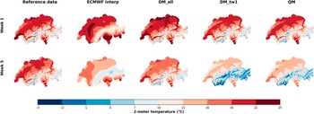
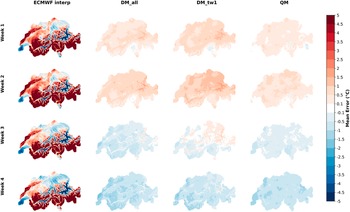
Both training strategies demonstrate a similar capability to downscale the ECMWF forecasts, producing spatially detailed temperature fields that exhibit patterns similar to those observed in the reference dataset (Figure 1). In terms of bias correction (Figure 2), complete bias removal remains challenging for all methods at these forecast ranges, particularly given the limited training data and the inherent uncertainty at longer lead times. Both DM approaches provide notable improvements of ME over the interpolated ECMWF data, although the improvements are somewhat smaller, though still comparable, to those achieved by QM. For lead weeks 1 and 2, the all-lead-time strategy (DM_all) outperforms the week 1–restricted approach (DM_tw1) over most of Switzerland, as indicated by smaller values of ME over most areas (Figure 2). In particular, for week 1 predictions, the all-lead-time approach reduces the ME by roughly twice as much as the week 1–restricted strategy, suggesting that the DM effectively exploits information from the daily week 1 lead times. For weeks 3 and 4, as well as for longer lead times not shown here (weeks 5 and 6), the week 1–restricted approach achieves a bias correction that is comparable to or slightly better than that of the all-lead-time strategy. However, as the differences between the two DM approaches are small for longer lead times, a larger sample size would be required to robustly assess their relative bias-correction performance. The similar bias correction observed for longer lead times between the two training strategies is partly attributable to the relative stability of weekly mean biases in the interpolated ECMWF forecasts at lead times longer than 2 weeks and to the small bias differences across the different lead weeks for several Swiss locations (see Supplementary Figure S1). Specifically, the bias can remain relatively stable either across all lead times (e.g., Zurich and Geneva in Supplementary Figure S1) or between shorter (first two weeks) and longer lead times (e.g., Locarno and Sion in Supplementary Figure S1). Although the DM_tw1 approach is trained on a smaller dataset than DM_all, it benefits from longer training time and is still exposed, through week 1 data, to bias magnitudes comparable to those at longer lead times. Moreover, the DM learns the overall data distribution rather than performing simple location-to-location adjustments, which likely contributes to its ability to generalize across lead times. It is also important to emphasize that the inputs to the DM consist of ECMWF forecasts interpolated from 36 km to 2 km resolution. This interpolation step can amplify the raw bias at all lead times, particularly over orographically complex regions. Moreover, the ECMWF model outputs are compared against observational data that were not seen during training. Consequently, discrepancies arising from resolution differences and the use of independent observational references may have a larger impact on model errors than the lead-time-dependent drift itself. The observed bias stability at specific locations and/or lead times is consistent with the results of Dutra et al. (Reference Dutra, Johannsen and Magnusson2021) (see their Figure 3a,b) that evaluate subseasonal ECMWF forecasts against fifth generation ECMWF atmospheric reanalysis (ERA5), the dataset used for the ECMWF model initialization (Vitart et al. Reference Vitart, Balsamo, Bidlot, Lang, Tsonevsky, Richardson and Alonso Balmaseda2019; Hersbach et al. Reference Hersbach, Bell, Berrisford, Hirahara, Horányi, Muñoz-Sabater, Nicolas, Peubey, Radu, Schepers, Simmons, Soci, Abdalla, Abellan, Balsamo, Bechtold, Biavati, Bidlot, Bonavita, De Chiara, Dahlgren, Dee, Diamantakis, Dragani, Flemming, Forbes, Fuentes, Geer, Haimberger, Healy, Hogan, Hólm, Janisková, Keeley, Laloyaux, Lopez, Lupu, Radnoti, de Rosnay, Rozum, Vamborg, Villaume and Thépaut2020).
Weekly 2 t from example forecasts initialized on 15 August 2020 (columns 2–5), together with the reference observational dataset (column 1). The panels display forecasts from the interpolated ECMWF IFS cycle 47r3 (second column), the DM_all approach (third column), the DM_tw1 approach (fourth column), and the QM approach (fifth column). The results are given for lead week 1 (first row) and lead week 5 (second row).
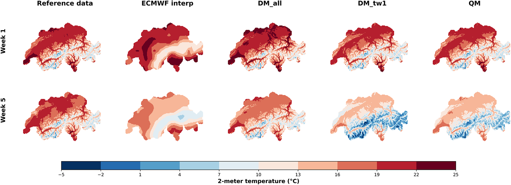
Figure 1. Long description
A grid of 10 geographical maps of Switzerland arranged in two rows and five columns.
Axes and Scale:
* The vertical axis labels the rows as Week 1 (top) and Week 5 (bottom).
* The horizontal axis labels the columns as Reference data, E C M W F interp, D M _ all, D M _ tw1, and Q M.
* A horizontal color bar at the bottom represents 2-meter temperature in degrees Celsius, ranging from minus 5 (dark blue) to 25 (dark red).
Data Distribution:
* Week 1 Row: The Reference data shows high temperatures (dark red) in the North and West, with cooler temperatures (light blue) in the Alpine regions of the South and East. The E C M W F interp model shows a smoothed, less detailed version of this pattern. The D M _ all, D M _ tw1, and Q M models closely replicate the high-resolution spatial details of the Reference data.
* Week 5 Row: The Reference data shows a similar but slightly cooler pattern than Week 1. The E C M W F interp model is very blurry, showing broad temperature zones. D M _ all maintains high-resolution detail similar to the reference. However, D M _ tw1 and Q M show significantly cooler temperatures (predominantly blue) in the Alpine regions compared to the Reference data, indicating a cold bias in these models at longer lead times.
Weekly 2 t ME derived from all model initializations between June and August 2020 for the interpolated ECMWF IFS cycle 47r3 (first column), the DM_all approach (second column), the DM_tw1 approach (third column), and the QM approach (fourth column). ME values closer to zero indicate a better score.
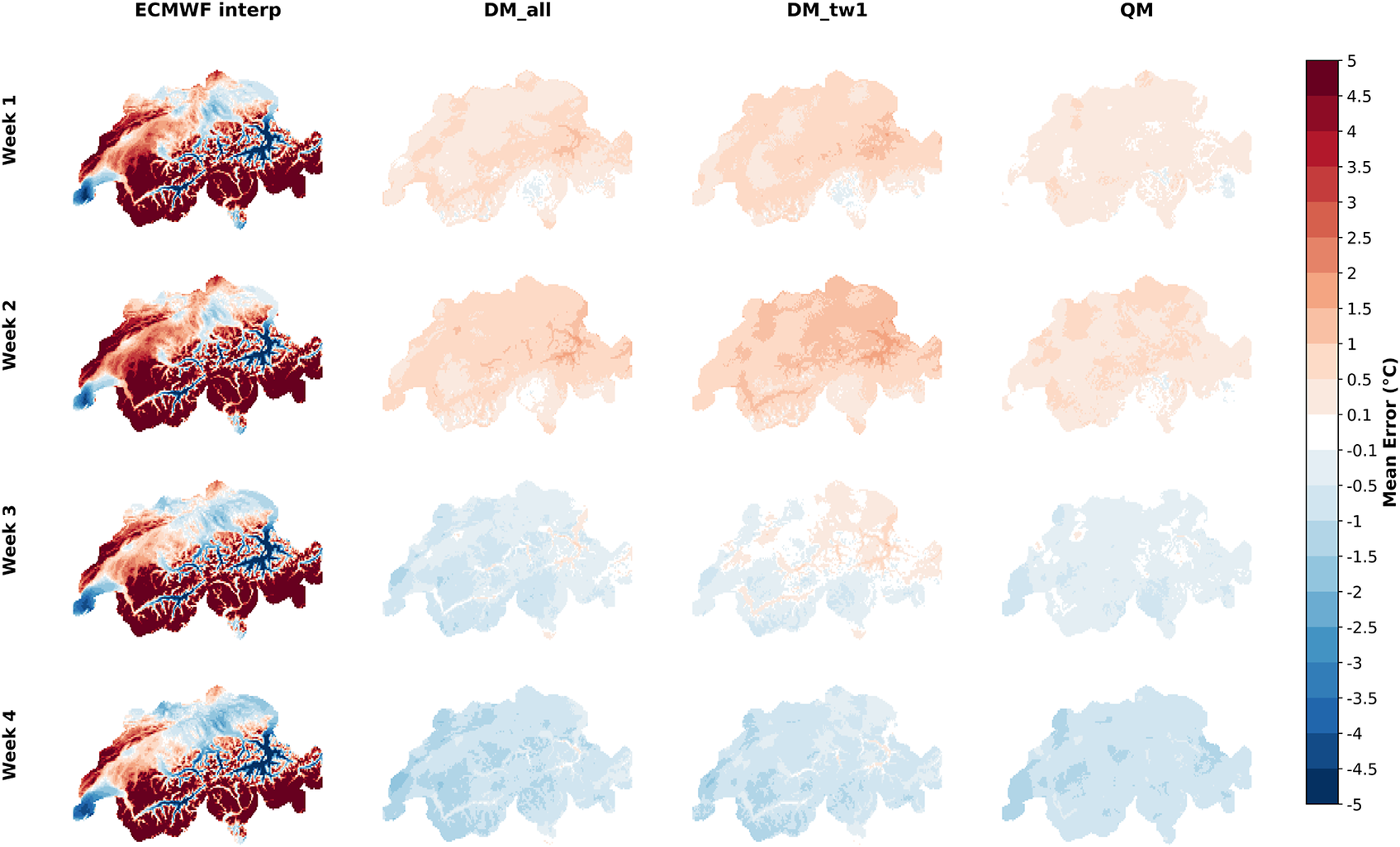
Figure 2. Long description
A multi-panel figure containing 16 maps of Switzerland arranged in four rows and four columns.
* Vertical Axis: Rows are labeled Week 1, Week 2, Week 3, and Week 4 from top to bottom.
* Horizontal Axis: Columns are labeled E C M W F interp, D M underscore all, D M underscore tw1, and Q M from left to right.
* Color Scale: A vertical legend on the right indicates Mean Error in degrees Celsius, ranging from negative 5 (dark blue) through 0 (white) to positive 5 (dark red).
Data Trends:
* Column 1 (E C M W F interp): Shows high intensity across all weeks, with deep red (positive error) in the southern and central regions and blue (negative error) in the northern and alpine areas.
* Column 2 (D M underscore all): Shows significantly reduced error compared to the first column. Week 1 and 2 are pale orange (slight positive error), while Week 3 and 4 shift toward pale blue (slight negative error).
* Column 3 (D M underscore tw1): Displays similar patterns to column 2 but with slightly more pronounced orange hues in the first two weeks.
* Column 4 (Q M): Shows the most neutral values (closest to white), indicating the lowest Mean Error across all four weeks, with very light blue shading appearing in Week 4.
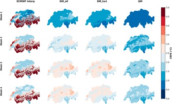
As Figure 2, but for the weekly 2 t CRPS. CRPS values closer to zero indicate a better score.
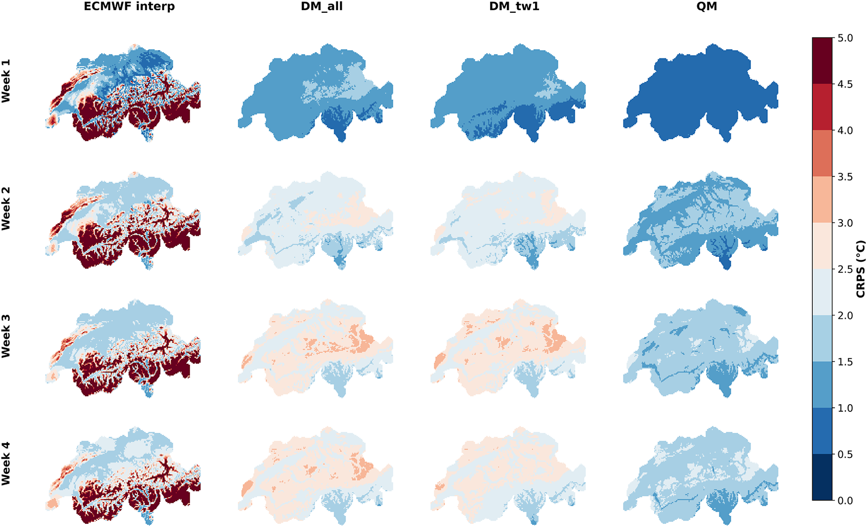
Figure 3. Long description
The grid consists of 16 maps of Switzerland. Columns are labeled E C M W F interp, D M _ all, D M _ t w 1, and Q M. Rows are labeled Week 1, Week 2, Week 3, and Week 4.
* A vertical color bar on the right indicates C R P S in degrees Celsius, ranging from 0.0 in dark blue to 5.0 in dark red. Values closer to zero represent better scores.
* The E C M W F interp column shows the highest C R P S values, with large areas of dark red concentrated in the South and West across all four weeks.
* The D M _ all and D M _ t w 1 columns show significantly lower C R P S values, appearing mostly in light blue and light orange, indicating improved performance over the interpolation model.
* The Q M column shows the lowest C R P S values in Week 1, dominated by dark blue. In Weeks 2 through 4, it transitions to light blue, maintaining a relatively low score compared to the first column.
* Across all models, the spatial distribution of error often follows topographical features, with higher C R P S values frequently appearing in the mountainous Southern regions.
The CRPS of the raw ECMWF forecasts is substantially reduced by both DM approaches, particularly over orographically complex regions, although the reduction is generally smaller than that achieved by QM (Figure 3). For lead week 1, the QM method reduces the raw ECMWF CRPS by nearly 1 °C over the Swiss Plateau and by more than 5 °C in complex terrain. The DM approaches reduce the ECMWF CRPS by approximately 0.5 °C over the Swiss Plateau and by about 4 °C over orographically complex regions, where the raw ECMWF CRPS reaches about 1 °C and exceeds 5 °C, for these regions, respectively. While the all-lead-time DM approach yields marginally lower CRPS improvements compared to the week 1–restricted strategy, the magnitude of the differences is small to support a statistically robust distinction between the two methods.
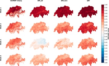
Finally, we assess the ability of the different approaches to predict hot extremes, defined as temperatures exceeding the observed 90th percentile (Figure 4). Discrimination skill is evaluated using the ROC/AUC score, where values of 0.5 or lower indicate no skill beyond random chance. The ROC/AUC metric accounts for both the hit rate and the false alarm rate across all possible decision thresholds, making it well suited for evaluating probabilistic predictions of extremes. Across all lead weeks, the QM approach attains AUC scores exceeding 0.7 in most of Switzerland. Although slightly lower, both DM strategies also demonstrate skill, with regional AUC values consistently above 0.5 for all lead weeks and both approaches, except for the all-lead-time strategy at lead week 3. From lead weeks 1 to 4, the week 1–restricted DM strategy generally outperforms the all-lead-time approach, whereas for lead weeks 5 and 6 (not shown), the all-lead-time strategy exhibits better discrimination. Across all methods, the ROC score generally decreases with increasing lead time from 1 to 6 weeks; however, both DM strategies display an unusually large reduction at lead week 3. A similar anomaly at lead week 3 is also evident in the CRPS (Figure 3) and may be related to the change in forecast resolution at this lead time in the ECMWF system (see Methods). For lead week 1, QM achieves the highest AUC, exceeding 0.95 for nearly all Swiss regions, followed by the DM approaches with regional values mostly above 0.9. This indicates that while QM performs best overall, both DM methods retain substantial skill in discriminating hot extremes across lead times.
As Figure 2, but for the weekly ROC/AUC score of 2 t extremes above the observed 90th percentile. ROC/AUC values closer to 1 indicate a better score, and values equal to or lower than 0.5 indicate no skill beyond random chance in discriminating between extreme and non-extreme events.
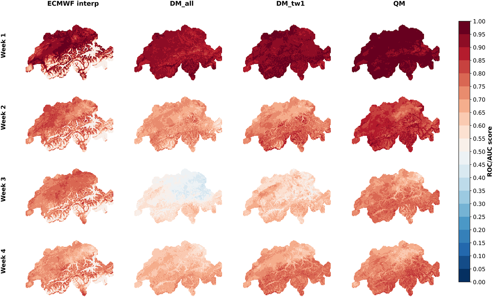
Figure 4. Long description
A multi-panel grid displays 16 maps of Switzerland arranged in four columns and four rows.
Columns from left to right are labeled: E C M W F interp, D M underscore all, D M underscore tw1, and Q M.
Rows from top to bottom are labeled: Week 1, Week 2, Week 3, and Week 4.
A vertical color bar on the far right indicates the R O C forward slash A U C score, ranging from 0.00 in dark blue to 1.00 in dark red. The midpoint of 0.50 is white, representing no skill.
Data trends:
* Week 1: All models show high skill with dark red and red shading across the entire country. E C M W F interp shows the highest values in the North.
* Week 2: Skill decreases across all models, transitioning to lighter red and orange hues. E C M W F interp shows white areas in the South, indicating lower skill in mountainous regions.
* Week 3: Skill continues to decline. D M underscore all shows a significant area of light blue in the North, indicating scores below 0.5. The other models remain in the light orange to white range.
* Week 4: Most maps show light orange to white shading, indicating low but positive skill, with Q M maintaining slightly higher red saturation than the other models.
Spatial distribution: Across all weeks and models, higher skill is generally concentrated in the Northern and Western regions, while the Southern Alpine regions often show lower scores, particularly in the E C M W F interp model.
Although DM_all is exposed to a larger training set, the inclusion of longer lead times (weeks 2–6), which are characterized by increased ensemble spread, results in a smoother ensemble mean used as training input. The competitive performance of DM_tw1 for longer lead times suggests that, despite being trained on a smaller dataset, it effectively leverages the higher signal-to-noise ratio of week 1 data. This indicates that the DM is able to learn the fundamental relationship between large-scale atmospheric conditions and fine-scale topographic features primarily from these high-quality inputs. Importantly, this learned relationship appears to generalize well to later lead times, even though the model is not explicitly trained on them.
4. Conclusion
This study introduces a generative diffusion-based framework for the simultaneous downscaling and bias correction of subseasonal temperature forecasts over complex terrain. By conditioning a probabilistic DM on coarse-resolution ECMWF subseasonal forecasts and explicitly incorporating lead-time information, we bias correct and downscale coarse horizontal resolution (36 km) ECMWF subseasonal hindcasts into high horizontal resolution (2 km) daily mean temperature fields over Switzerland. The proposed approach generates physically plausible, high-resolution temperature fields while simultaneously accounting for forecast uncertainty through ensemble sampling. Both of these aspects are important for impact-oriented applications.
We have evaluated two distinct training strategies on a univariate 2 t model. Specifically, the all-lead-time approach reduces the ME in week 1 predictions by approximately 50% more compared to the week 1–restricted strategy. For longer lead times, both methods show comparable performance, likely due to the relative stability of weekly mean biases in the underlying coarse-resolution forecasts as compared to the reference dataset that was never seen by the model and is based on spatially interpolated observations. While the baseline QM method retains an advantage in terms of CRPS and extreme event discrimination (ROC/AUC), the DMs successfully reduce raw ECMWF CRPS by up to 4 °C in orographically complex regions. QM’s strong performance reflects its targeted optimization of marginal distributions, making it a difficult baseline to outperform, particularly in probabilistic verification metrics.
A key contribution of this work is the explicit examination of lead-time conditioning and training strategies in generative downscaling for the subseasonal range. By contrasting an all-lead-time training strategy with a week 1–restricted approach, we show that DMs can flexibly correct bias structures across lead times, while remaining robust even when trained on relatively limited datasets. Importantly, our results indicate that effective subseasonal post-processing does not necessarily require extensive training data across all lead times, making the approach attractive for applications where data availability or computational resources are constrained. Beyond forecast skill, the proposed framework offers advantages for operational use. Unlike traditional QM, the DM generates its own ensemble from a single forecast input, reducing storage needs and enabling relatively fast inference (50 members in 40 minutes on a single GPU). In addition, its generative design allows new predictors or variables to be easily incorporated, facilitating extension to other surface variables or challenging regimes such as wintertime temperature inversions.
While this study focuses on summer temperature forecasts over Switzerland, chosen as a challenging test case due to strong orographic effects and pronounced summer biases, the methodological insights are broadly transferable. The proposed diffusion-based framework is not tied to a specific model cycle, geographic region, or atmospheric variable and is therefore expected to remain applicable as dynamical forecasting systems continue to evolve. In this work, the DM is conditioned on the ensemble-mean forecast in order to isolate and systematically evaluate the impact of the two training strategies on bias-correction performance. This design choice, however, may limit the generalization of the model and its ability to fully represent ensemble spread.
Several promising avenues for future development, therefore, emerge from this study. Training the DM on all ensemble members or on a single forecast (e.g., control forecast) could improve the representation of forecast uncertainty and extremes and potentially enhance probabilistic skill. In addition, jointly training across multiple initialization dates may improve generalization across atmospheric regimes while retaining lead-time awareness. Further extensions could include multivariate downscaling, incorporation of additional physical predictors, or the prediction of impact-relevant indices. Although these developments are beyond the scope of the present work, they represent natural and well-motivated next steps toward fully exploiting diffusion-based generative models for subseasonal forecasting.
Overall, this work provides a concrete and operationally relevant benchmark for applying lead-time-informed diffusion-based generative models to subseasonal forecasting. It demonstrates that such models can effectively bridge the gap between coarse-resolution dynamical forecasts and the high-resolution probabilistic information required for impact-oriented applications, thereby contributing a practical tool to the growing field of climate informatics.
Supplementary material
The supplementary material for this article can be found at http://doi.org/10.1017/eds.2026.10047.
Data availability statement
ECMWF IFS hindcast data are available from the ECMWF public data archive at https://apps.ecmwf.int/archive-catalogue/. The observational TabsD dataset can be accessed through MeteoSwiss’ Open Government Data infrastructure (https://www.meteoschweiz.admin.ch/service-und-publikationen/service/open-data.html). The DM code is publicly available at https://github.com/marpyr/Diffusion_Downscaling.
Acknowledgments
We acknowledge financial support from the Swiss drought program (https://www.meteoswiss.admin.ch/about-us/research-and-cooperation/projects/2024/drought-program.html). We extend our gratitude to MeteoSwiss for the access to the TabsD observational products, as well as the subseasonal forecast archive. M.P. and D.B. acknowledge financial support from the Collaborative Research on Science and Society (CROSS) program of École Polytechnique Fédérale de Lausanne (EPFL) and Université de Lausanne (UNIL). This project has received funding from the European Research Council (ERC) under the European Union’s Horizon 2020 research and innovation program (grant agreement no. 847456) and from a grant from the Swiss National Supercomputing Centre (CSCS) under project ID s1144. We would also like to thank and acknowledge Joffrey Dumont Le Brazidec (ECMWF), Maxim Samarin (Swiss Data Science Center), Jakob Schloer (ECMWF), and Steffen Tietsche (ECMWF) for fruitful discussions.
Author contributions
M.P. conceptualized and conducted the study, built the DM, analyzed and visualized the data, and wrote the original manuscript draft. A.I. provided the hindcast data and quantile-mapped forecasts and conceptualized the study. D.B. conceptualized the study. C.S. and D.D. acquired funding, conceptualized the study, and supervised the study. All authors reviewed the manuscript.
Competing interests
The authors confirm that they have no competing interests.
Ethics statement
The research meets all ethical guidelines, including adherence to the legal requirements of the study country.
Provenance statement
This article is part of the Climate Informatics 2026 proceedings and was accepted in Environmental Data Science on the basis of the Climate Informatics peer-review process.


 Open access

