


1. Introduction
Transition in hypersonic (Mach number >5) boundary layers is a key issue in the realisation of hypersonic flight because it causes a significant increase in aerodynamic heating, entropy production and uncertain aerodynamic forces. An in-depth understanding of the transition mechanism is vital to improving the performance and safety of hypersonic vehicles. Much attention has been paid to transition over three-dimensional (3-D) configurations due to its strong relevance to realistic hypersonic vehicles. Related 3-D geometries that have previously been investigated include bodies of rotation at non-zero angles of attack (Ward, Henderson & Schneider Reference Ward, Henderson and Schneider2015; Craig & Saric Reference Craig and Saric2016), elliptic cones (Kimmel et al. Reference Kimmel, Adamczak, Juliano and Paull2013), the lifting body (Chen et al. Reference Chen, Tu, Wan, Yuan, Yang, Zhuang and Xiang2021b) and the delta wing model (Niu et al. Reference Niu, Yi, Liu, Lu and He2019). These 3-D bodies are subject to an azimuthal or spanwise pressure gradient that transfers fluid from a high-pressure to a low-pressure region. Streamlines connecting the two regions are often curved so that they are conducive to stationary/travelling cross-flow instabilities (Borg & Kimmel Reference Borg and Kimmel2016; Dinzl & Candler Reference Dinzl and Candler2017; Yates et al. Reference Yates, Juliano, Matlis and Tufts2018; Cerminara & Sandham Reference Cerminara and Sandham2020; Tufts et al. Reference Tufts, Borg, Bisek and Kimmel2022). In addition, the oblique second mode, rather than its planar counterpart (Mack Reference Mack1969), is possibly present in 3-D boundary layers (Balakumar & Reed Reference Balakumar and Reed1991; Moyes et al. Reference Moyes, Paredes, Kocian and Reed2017, Reference Moyes, Kocian, Mullen and Reed2018; Tufts et al. Reference Tufts, Borg, Bisek and Kimmel2022). Transition in 3-D hypersonic boundary layers is much more complex than in 2-D boundary layers, in terms of linear instabilities, nonlinear interactions and flow structure evolution.
In the linear stage, there exist at least two types of cross-flow instability in 3-D boundary layers, called the stationary or travelling cross-flow instabilities. It is well known that under incompressible conditions, the initial amplitudes of stationary and travelling cross-flow instabilities are, respectively, dominated by the surface roughness and unsteady disturbances. Therefore, transition in low-disturbance flows is more relevant to stationary cross-flow instabilities (Gray Reference Gray1952; Reed & Lin Reference Reed and Lin1987; Saric Reference Saric1992, Reference Saric1994; Malik, Li & Chang Reference Malik, Li and Chang1994; Kachanov Reference Kachanov1996; Saric, Reed & White Reference Saric, Reed and White2003). Similar conclusions were reached for hypersonic flows based on a tremendous number of wind tunnel experiments and numerical simulations (Borg, Kimmel & Stanfield Reference Borg, Kimmel and Stanfield2011, Reference Borg, Kimmel and Stanfield2012, Reference Borg, Kimmel and Stanfield2013; Ward et al. Reference Ward, Henderson and Schneider2015; Craig & Saric Reference Craig and Saric2016; Corke et al. Reference Corke, Arndt, Matlis and Semper2018; Edelman & Schneider Reference Edelman and Schneider2018; Arndt et al. Reference Arndt, Corke, Matlis and Semper2020; Yates et al. Reference Yates, Matlis, Juliano and Tufts2020) and, thus, the stationary cross-flow instabilities have received most of the attention in previous studies because of their significance to real flight conditions in which the disturbance level is very low. However, some recent evidence has demonstrated the existence of travelling cross-flow instabilities in hypersonic transitions, indicating an underlying significance to transition. Borg, Kimmel & Stanfield (Reference Borg, Kimmel and Stanfield2015) investigated flows over an elliptic cone in a Mach 6 quiet wind tunnel. This kind of wind tunnel can provide a free-stream disturbance level as low as that under real flight conditions. The travelling cross-flow instability waves were detected using pressure sensors flush-mounted on the surface. The phase speed and the wave angle of the instability waves were calculated from the cross-spectra of the three pressure sensors and showed good agreement with linear stability theory. Similar results were then numerically reproduced by Tufts et al. (Reference Tufts, Borg, Bisek and Kimmel2022) which proved the observation by Borg et al. (Reference Borg, Kimmel and Stanfield2015). More persuasive evidence came from a recent real flight test by Wan et al. (Reference Wan, Tu, Yuan, Chen and Zhang2021), which proved the existence of the travelling cross-flow instability in the transition process. All of these results show that the role of the travelling cross-flow instabilities in hypersonic transitions is worthy of deep further study for practical purposes.
Interactions between travelling cross-flow instabilities with other instabilities have also been reported. Munoz, Heitmann & Radespiel (Reference Munoz, Heitmann and Radespiel2014) experimentally investigated instabilities over a 7 $^\circ$ half-angle cone at an angle of attack of 7 $^\circ$ in a Mach 6 wind tunnel using surface-mounted PCB $^\circledR$ sensors. A bi-coherence peak was identified between the second mode and the travelling cross-flow vortices, showing a nonlinear interaction between them. Similar results were also obtained by Ward et al. (Reference Ward, Henderson and Schneider2015), Craig & Saric (Reference Craig and Saric2016). Numerical simulations under similar conditions were also conducted by Choudhari et al. (Reference Choudhari, Li, Paredes and Duan2017) and Dong et al. (Reference Dong, Chen, Yuan, Chen and Xu2020), showing that the second mode was easily destabilised both by stationary and travelling cross-flow vortices. Dong et al. (Reference Dong, Chen, Yuan, Chen and Xu2020) pointed out that these modulated the second modes may have a significant influence on the onset of transition. Recently, Chen et al. (Reference Chen, Dong, Tu, Yuan and Chen2022) studied the instability of the boundary layer over a lifting body model (HyTRV) by using global stability and linear parabolised stability equations. They found that the cross-flow mode dominated in the windward region whereas the second mode and the cross-flow mode coexisted in the shoulder region, and only the unstable second mode was found along the attachment line. Interactions between the second mode and cross-flow instabilities were also observed. However, detailed information on these instability interactions is still quite limited.
From a structural aspect, a prominent characteristic of the cross-flow instability is the appearance of stationary or travelling cross-flow vortices. Experimentally, stationary vortices can be observed as time-averaged streak structures using surface temperature measurements or oil-flow visualisation, while travelling ones are much more difficult to visualise. Niu et al. (Reference Niu, Yi, Liu, Lu and He2019) investigated the cross-flow instability over a delta flat plate at Mach 6. The model's flat surface was convenient for planar laser diagnostics to capture the flow structure of travelling cross-flow vortices at the frequency of 14 kHz. Secondary finger structures were also observed connecting to one primary cross-flow vortex, and these were noted to be similar to previous observations of travelling cross-flow vortices in low-speed flows (Wassermann & Kloker Reference Wassermann and Kloker2003). Chen et al. (Reference Chen, Dong, Chen, Yuan and Xu2021a) also found such secondary finger structures connecting to one primary stationary vortex over a Mach 6 swept wing. By comparison with a stability analysis, the secondary structures were identified as the action of the  $z$-type secondary instability mechanism. New footprint structures attached to the wall that had the same frequency as the secondary finger structures were also discovered along the direction normal to the streamwise direction. However, no deep explanation of this footprint structure was given.
The motivation for this work is to investigate the transition over a delta wing model at Mach 6.5, in terms of interactions between different unstable modes and related evolution of flow structures. A combination of experiments and direct numerical simulations (DNS) is applied to study the time-resolved evolution of transitional flow structures. Experimentally, a double-pulsed illumination-imaging system with a repetition rate of 10 Hz, as well as an 8-pulsed ultra-fast image acquisition system with a repetition rate of 100 kHz, is used to capture the flow structure (Thurow et al. Reference Thurow, Hileman, Samimy and Lempert2002, Reference Thurow, Jiang, Kim, Lempert and Samimy2008). A high-speed schlieren technique is applied (Laurence, Wagner & Hannemann Reference Laurence, Wagner and Hannemann2016), which for the first time captures the global evolution of unstable modes on a delta flat plate. Numerically, detailed information on the 3-D flow structure evolution and its underlying mechanism is further investigated using simulations. This paper is organised as follows. The experimental and numerical settings are introduced in § 2. The results of the ultra-fast experiments, schlieren experiments and numerical simulations are presented in § 3. Analyses and discussions about the nonlinear interaction of different modes and the generation of the secondary structure are presented in § 4. A summary and concluding remarks are provided in § 5.
2. Experimental set-up
2.1. Quiet wind tunnel and experimental model
The experiment was conducted in the hypersonic  $\varPhi 300$ mm quiet wind tunnel of Peking University under noisy conditions with an incoming Pitot pressure pulsation of about 1 %. The incoming Mach number, the total temperature, the total pressure and the corresponding unit Reynolds number are 6.5, 410 K, 1.06 MPa and $1 \times 10^7$ m $^{-1}$, respectively. The model used in the experiment is a delta wing model with a sweep angle of 75 $^\circ$, a length of 400 mm, a thickness of 7 mm and a front-edge radius of 3.5 mm (figure 1). The coordinate origin is located at the apex of the delta wing with $x$ being the streamwise direction along the centreline, $y$ being normal to the surface and $z$ obeying to a right-hand system of $x$ and $y$, with the velocity components $u$,
$u$,  $v$ and $w$ along the $x$,
$x$,  $y$ and $z$ directions, respectively. A local coordinate is also applied with $x_t$ parallel to the inviscid streamline at the boundary layer edge and $z_t$ normal to the $x_t$– $y$ plane. The velocity component $u_t$ (the so-called tangent velocity) and $w_t$ (the so-called cross-flow velocity) are respectively along the $x_t$ and $z_t$ directions.

Figure 1. (a) A schematic diagram of the delta wing model used in the pressure sensor measurement. The coordinates of the PCB installation position are from  $x = 232.5$ mm to 377.5 mm with an intervals of 14.5 mm and from $z = 45.1$ mm to 6.5 mm with an interval of $-$3.8 mm. (b) Schematic diagram of the delta wing model used in the high-speed schlieren experiment. The upper part of the delta wing model is inlaid with quartz glass. (c) Schematic diagram of the high-speed schlieren set-up. Ultra-fast flow visualisation set-up with laser parallel to the (d) $x$–
$x$– $z$ and (e) $y$–
$y$– $z$ section of the model surface.
2.2. Rayleigh scattering flow visualisation technology
The flow visualisation system contains an ultra-fast camera and an eight-channel high-energy pulsed laser system. The nominal spatial resolution of the ultra-fast camera is  $2048 \times 2048$ pixels. The camera view is divided into four independent internal channels, and each channel can work in single-exposure or double-exposure mode. Therefore, a 333 MHz or 2 MHz sample can obtain the rate of four image series (single exposure mode) or eight image series (double exposure mode). The illumination system is an eight-channel high-energy pulsed laser system, which outputs laser pulses of 200 mJ energy and 10 ns duration. The timing of the camera and the laser is precisely controlled by a 48-channel synchronisation system that emits a transistor–transistor logic (TTL) square-wave packet (including eight square-wave signals) every 100 ms (corresponding to a repetition rate of 10 Hz).
By using CO $_2$ Rayleigh scattering flow visualisation, the clear flow field structure information near the boundary layer can be obtained. CO $_2$ is added upstream of the nozzle. When the static temperature of the test section is lower than 50 K, CO $_2$ condenses into solid particles, which can be viewed by Rayleigh scattering under the light of a laser sheet. Within the boundary layer, the CO $_2$ is gaseous due to vaporisation by the aerodynamic heating of the boundary layer. CO $_2$ gas is injected upstream of the test section. The mass injection rate of CO $_2$ is no more than 5 % of the freestream flow. This technology was first used at Princeton University to observe the hypersonic turbulent boundary layer and the interaction between a shock and boundary layer (Poggie & Smits Reference Poggie and Smits1996; Erbland et al. Reference Erbland, Baumgartner, Yalin, Etz, Muzas, Lempert, Smits, Miles, Erbland and Baumgartner1997; Smits & Lim Reference Smits and Lim2000). Zhang et al. (Reference Zhang, Zhu, Chen, Yuan, Wu, Chen, Lee and Gad-El-Hak2015) used this technology to obtain a clear picture of the complete process of hypersonic boundary layer transition.
2.3. Infrared thermography
The surface temperature of the model is measured using an FLIR $^\circledR$ T 620 infrared (IR) camera. The camera has a resolution of $640 \times 480$ pixels, a thermal sensitivity of 0.05 K or better, a shooting frequency of 30 Hz, a detection wavelength range of 7.5–14 $\mathrm {\mu }$m and a detection temperature range between $-40$ and 650 $^\circ$C.
2.4. Disturbance measurement
Surface-mounted PCB $^{\circledR }$ fast-response sensors have proven to be convenient tools for evaluating the evolution of instability waves in hypersonic wall-bounded flows (Zhu et al. Reference Zhu, Zhang, Chen, Yuan, Wu, Chen, Lee and Gad-el Hak2016) by detecting pressure fluctuations. In this work, PCB $^{\circledR }$ 132A31 sensors are flush mounted along one ray of the model. The sensor is a piezoelectric quartz sensor with a high-frequency response above 1 MHz and a minimum resolution of 7 Pa. The sensors are high-pass filtered, so they only measure fluctuations above 11 kHz. The diameter of the sensor's head is 3.18 mm, but the effective sensing area is only about 0.581 mm $^2$. The coordinates of the PCB installation position are from $x = 232.5$ mm to 377.5 mm with an interval of 14.5 mm and from $z = 45.1$ mm to 6.5 mm with an interval of $-$3.8 mm. The signals of the PCB $^{\circledR }$ sensors are first processed by ICP $^{\circledR }$ signal conditioners and then recorded by the acquisition system with a sample rate of 1 MHz.
High-speed schlieren technology that uses a high-speed camera can work at a very high sampling frequency, and it is now commonly used to measure spatiotemporal high-speed flow fields (Laurence et al. Reference Laurence, Wagner and Hannemann2016). This experiment uses a typical Z-shaped optical path (figure 1c). The light source is a 532-nm continuous LED with a power of 150 W. To ensure the quality of the light source, the light is emitted through a small hole with a diameter of 1.5 mm before reaching paraboloid schlieren mirrors, mirrors 1 and 2, which have a diameter of 300 mm and a focal length of 3 m. The camera is a Phantom v2512 camera, combined with a Nikon 200-mm lens. To obtain a sample frequency of 380 kHz, the camera's resolution is reduced to  $256 \times 128$ pixels. The schlieren knife edge is placed vertically so that the schlieren signal is a function of $\partial \rho /\partial x$. During the experiment, part of the model surface is replaced with optical glass (figure 1b). The model is placed vertically, as shown in figure 1(c), so that the light can pass through the delta wing model along the wall-normal direction. The amplitude, spectrum, convection direction and speed of the instabilities can be derived from the schlieren image series following the data processing method described in Appendix A.
3. Numerical set-up
3.1. Basic set-up for the DNS
The model used in the calculation is the same as the experimental model and is shown in figure 2. The delta wing model is 7 mm thick, 400 mm long, with a sweep angle of 75 $^\circ$ and a rounded leading edge design. The flow conditions are as follows: the incoming Mach number is 6.5, the static pressure is 395 Pa, the total temperature is 410 K and the unit Reynolds number is $9.7 \times 10^6$ m $^{-1}$. The simulation includes three steps: the first step is to calculate the head of the delta wing (A in figure 2), the second step is to calculate the rest of the surface flow including the shock wave (B in figure 2) and the third step focuses on the boundary layer area behind the shock wave (C in figure 2) so as to precisely simulate the boundary layer flow, which is main concern of this study. For part A, the number of flow direction, normal direction, and spanwise grid points is $N_x\times N_y\times N_z = 120\times 200\times 60$. The convection term is discretised using the MUSCL scheme, the viscous term is discretised by fourth-order central difference scheme, the inlet condition is a free incoming flow, the outlet condition is an extrapolated boundary condition and the symmetrical boundary condition is adopted at the centreline and leading edge. To handle the singularity near the nose, a quasi-axial-symmetry mesh grid is adopted where the first layer slightly deviates the axis, as shown in figure 2. The boundary conditions upstream of the nose are that the second derivative of all primary variables is zero. For part B, the number of grid points in the flow direction, normal direction, and spanwise direction is $N_x\times N_y \times N_z = 800 \times 150 \times 150$. The convection term and the viscous term are discretised by the same methods as in part A. The inlet condition arises from the natural neighbour interpolation of the results of part A. The exit condition is also an extrapolation boundary condition. No disturbance is added to part A or part B.

Figure 2. A schematic diagram of the DNS set-up. The green region represents the blowing and suction port on the model surface where the initial disturbance is added. The blowing and suction port is divided into two parts. The first part (light green) is approximately parallel to the intersection of the inlet of part C and the surface, covering the streamwise grid numbers from  $k_{x1} = 140$ ( $x \simeq 25$ mm) to $k_{x1} = 190$ ( $x \simeq 35$ mm) and the spanwise grid numbers from 1 ( $z = 0$ mm or the centreline) to 300 (leading edge). The second part (dark green) is approximately parallel to the leading edge, covering the streamwise grid numbers from $k_{x3} = 190$ ( $x \simeq 35$ mm) to $k_{x4} = 1700$ ( $x \simeq 380$ mm) and the spanwise grid numbers from $k_{z1} = 220$ to $k_{z1} = 295$.
For part C, the convection term is treated using the Steger–Warming flux vector splitting method and then discretised using the seventh-order weighted essentially non-oscillatory (WENO) scheme. The viscous term is discretised by an eighth-order central difference scheme. The Runge–Kutta method of third-order total variation differentiation (TVD) is adopted for time stepping. The inlet conditions and upper boundary conditions are calculated in the second step through natural neighbour interpolation. The symmetrical boundary conditions are adopted at the centreline and leading edge, and the extrapolated boundary conditions are kept at the outlet. The wall conditions used in the simulation are no-slip and isothermal boundary conditions ( $u = v = w = 0$, $T = 6.5 T_0$, $\partial p/ \partial n = 0$) (Pirozzoli & Grasso Reference Pirozzoli and Grasso2004; Li, Fu & Ma Reference Li, Fu and Ma2010) because the stainless steel model used in the wind tunnel experiment is closer to the isothermal wall.
Three grid sizes are applied to verify the grid independence, as indicated by table 1. Their numbers of grid points in the flow direction, normal direction and spanwise direction are  $N_x\times N_y \times N_z = 1000\times 100 \times 200$ for the low resolution, $N_x\times N_y \times N_z = 1700 \times 150 \times 300$ for the medium resolution and $N_x \times N_y \times N_z = 2000 \times 200 \times 400$ for the high resolution, respectively. The minimum length scale in the wall-normal direction, denoted as ${\rm \Delta} y^+_{min}$, is also presented in table 1 and is calculated using the formula
 \begin{equation} y^+{=}\frac{y}{\delta_{\nu}}=\frac{y\sqrt{\dfrac{\tau_w}{\bar{\rho}_w}}}{\nu}, \end{equation}
where the superscript  $^+$ represents the wall scale, $y$ refers to the wall-normal distance, $\nu$ refers to the viscosity, $\bar {\rho }_w$ refers to the average density and $\tau _w$ refers to the wall shear stress. Table 1 indicates that, for both the medium- and high-resolution grids, ${\rm \Delta} y^+_{min}$ is less than 1, whereas for the low-resolution grid ${\rm \Delta} y^+_{min}$ is larger than 1. A comparison of the basic flows obtained from the three grids is presented in figure 3. The wall-normal distance $y$, the tangent velocity $u_t$, the cross-flow velocity $w_t$ and the temperature are normalised by the $99\,\%$ tangent velocity boundary layer thickness $y_{99}$, the free-stream velocity $u_0$, a tenth of free-stream velocity $0.1u_0$ and 10 times free-stream temperature $10T_0$, respectively. It can be seen that the tangent velocity and the temperature profiles are almost the same among all three grids for different locations. However, a prominent deviation of the cross-flow velocity for the low resolution can be observed from the other two resolutions when the streamwise position is at 350 mm (see the orange lines in figure 3a). To further verify the grid independence, the profiles of $\hat {u}$ for the travelling cross-flow mode are compared between the medium- and high-resolution grids among different locations, as shown in figure 4. A good agreement on disturbances field between the two grids is obtained as well. Since the error rate between the medium- and high-resolution grids is less than $5\,\%$ for all results, we adopt the medium-resolution grid when considering calculation costs.
Table 1. Mesh grids for the calculation of part C.


Figure 3. A comparison of the basic flow profiles among the different grids. (a) The cross-flow velocity profiles  $-10 w_t/u_0$. (b) The tangent velocity profiles $u_t/u_0$. (c) The temperature profile $0.1T/T_0$. The low, medium, and high resolutions correspond to $N_x\times N_y \times N_z = 1000\times 100 \times 200$, $N_x\times N_y \times N_z = 1700 \times 150 \times 300$ and $N_x \times N_y \times N_z = 2000 \times 200 \times 400$, respectively. Different colours represent the alteration of the position. The blue, red and orange lines are at the delta wing $(x, z) = (150\ {\rm mm}, 30\ {\rm mm})$, $(x, z) = (250\ {\rm mm}, 30\ {\rm mm})$ and $(x, z) = (350\ {\rm mm}, 30\ {\rm mm})$, respectively. The vertical coordinates are normalised by the boundary layer thickness.

Figure 4. A comparison of the profiles of  $\hat {u}$ for the travelling cross-flow mode between the medium- and high-resolution grids. (a) At the delta wing $(x, z) = (150\ {\rm mm}, 30\ {\rm mm})$. (b) At the delta wing $(x, z) = (250\ {\rm mm}, 30\ {\rm mm})$. (c) At the delta wing $(x, z) = (350\ {\rm mm}, 30\ {\rm mm})$.
The cross-flow velocity, tangent velocity and temperature profiles of the basic flow from the calculation on the medium-resolution grid are then shown in figure 5. The sample locations are along the planes  $z = 30$ mm and $x = 190$ mm, which are indicated by the blue and red dotted lines in figure 5(a). It can be seen that there is good agreement in the tangent velocity (figure 5c,f) and temperature profiles (figure 5d,g) at all locations, whereas the maximum of the cross-flow velocity decreases with the streamwise coordinate $x$ for $z = 30$ mm (figure 5b) and increases with the spanwise coordinate $z$ for $x = 190$ mm. In other words, the maximum cross-flow velocity increases as the location approaches the leading edge, which indicates that the cross-flow waves mainly appears in the region near the leading edge, benefiting the easy growth of cross-flow instability.

Figure 5. (a) The basic flow profiles along  $z = 30$ mm and $x =190$ mm indicated by the blue and red dotted lines, respectively. (b,e) The cross-flow velocity profiles $-10 w_t/u_0$. (c,f) The tangent velocity profiles $u_t/u_0$. (d,g) The temperature profile $0.1T/T_0$. The locations for (b–d) are $x = 150$ mm, 190 mm, 230 mm, 270 mm, 310 mm and 350 mm along the blue dotted line $z = 30$ mm. The locations for (e–g) are $z = 25$ mm, 35 mm, 45 mm and 55 mm along the red dotted line $x = 190$ mm. Here $u_t$, $w_t$, $T$,
$T$,  $u_0$ and $T_0$ are the tangent velocity, cross-flow velocity, temperature, freestream velocity and freestream temperature, respectively.
3.2. Linear stability theory analysis set-up
The stability characteristics of the basic flow are then investigated using the linear stability theory, in a manner similar to that in the study of Chen, Zhu & Lee (Reference Chen, Zhu and Lee2017b). The decomposition of the flow field is given by
 \begin{equation} q(x,y,z,t)=\bar{q}(y)+ q^\prime(y)=\bar{q}(y)+ \hat{q}(y)\exp({\rm i}\alpha x+{\rm i}\beta z-{\rm i}\omega t)+{\rm c.c.} \end{equation}
Here,  $q=(u, v, w, T, p)$ and $\bar {q}$ denote the basic states, $q^\prime$ denotes the disturbance, $\hat {q}(y)$ is the shape function of the disturbance, $\alpha$ and $\beta$ represent the streamwise wavenumbers and the spanwise wavenumbers, respectively, and $\omega$ is the angular frequency. In this study, the basic state is given by DNS and is partly presented in figure 5.
After substituting the decompositions given by (3.2) into the Navier–Stokes equations, subtracting the basic states and neglecting the non-parallel and nonlinear terms, the following eigenvalue problem is obtained:
 \begin{equation} L_1(x,\alpha, \beta, \omega)\hat{q}(y) = 0. \end{equation}
 Here  $L_1$ is a linear operator that has been described in previous literature (Chen et al. Reference Chen, Zhu and Lee2017b) and the flow parameters are the same as in the experiment. When considering the temporal formula, we have
 \begin{equation} \omega=\omega(\alpha,\beta), \end{equation}
where  $\omega$ is complex, $\alpha$ and $\beta$ are real. When considering the spatial formula, we have
 \begin{equation} \alpha=\alpha(\omega,\beta), \end{equation}
where  $\alpha$ is complex, $\omega$ and $\beta$ are real. For the smooth-wall PEEK model, the boundary conditions are
 \begin{equation} \hat{u}=\hat{v}=\hat{w}=\frac{{\partial \hat{T}}}{\partial \eta}=0 \ {\rm at}\ \eta=0, \quad \hat{u}=\hat{v}=\hat{w}= \hat{T}=0 \ {\rm at}\ \eta \rightarrow \infty. \end{equation}
The analysis in this study is carried out with the spatial formula using the in-house code in our laboratory; see the work of Chen, Zhu & Lee (Reference Chen, Zhu and Lee2017a) for the specific calculation method and code verification. Figure 6 shows the results of the linear stability analysis of the spatial model at different locations. It shows that the second mode wave disturbance appears near a frequency of 120 kHz, whose spanwise wavenumber approaches zero. The travelling cross-flow mode appears near a frequency of 50 kHz while the spanwise wavenumber is positive. The instability at low frequency and negative spanwise wavenumber appears only near the leading edge, which has a low growth rate and high phase speed (about 1.5 mainstream velocity). It will not be discussed in this article. The wave angle of the cross-flow mode is  $-20^{\circ }$.

Figure 6. Variation of spatial growth rate with frequency and spanwise wavenumber at different position.
A well-known, unique characteristic of the second mode is its large velocity disturbance below the sonic line, which is clearly shown by a black arrow in figure 7(a). This large disturbance is caused by the periodic compression–expansion motion, which was discussed by Zhu et al. (Reference Zhu, Zhang, Chen, Yuan, Wu, Chen, Lee and Gad-el Hak2016). The following discussion uses the disturbance profile beneath the sonic line as a criterion for identifying the presence of the second mode.

Figure 7. A comparison of the disturbance profiles between the DNS and linear stability theory results at position  $(x, z) = (170\ {\rm mm}, 30\ {\rm mm})$. (a) The second mode. (b) The travelling cross-flow mode. The arrow in panel (a) points to the location where the disturbance reaches its maximum value. The black dashed line represents the sonic line.
3.3. Disturbance set-up for DNS
When considering the disturbance field, following the results of the PCB pressure measurement experiment, disturbances with frequencies of 48 and 118 kHz, different spanwise wavenumbers and different streamwise wavenumbers are added to the wall near the leading edge inlet in the simulation. The disturbance of  $\omega _1 = 48$ kHz introduces the travelling cross-flow wave and the disturbance of $\omega _2 = 118$ kHz introduces the second mode. In this case, the disturbance of the Mack's first mode (22 kHz) is not added. The unsteady blowing and suction disturbance is added near the inlet and at the edge of the delta wing (the green area in figure 2). The form of the disturbance is as follows:
 \begin{gather} v_n = Av_{dis_x} v_{dis_z}v_{fre}v_{shape}, \end{gather}
 \begin{gather}v_{dis_x} = \frac{1}{50}\sum_{i=1}^{50} \sin\left(\frac{2 {\rm \pi}x}{i}\right), \end{gather}
 \begin{gather}v_{dis_z} =\frac{1}{10} \sum_{i=1}^{10} \sin{\left(\frac{2{\rm \pi} z}{i}\right)}, \end{gather}
 \begin{gather}v_{fre} = ( A_1\sin{(\omega_{1} t)} + A_2\sin{(\omega_{2} t)}), \end{gather}
 \begin{gather}v_{shape1} = \sin^{3} \left(\frac{{\rm \pi} (k_{x}-k_{x 1})}{k_{x 2}-k_{x 1}}\right), \end{gather}
 \begin{gather}v_{shape2} = \sin^{3}{\left(\frac{{\rm \pi} (k_{z} - k_{z 1})}{k_{z 2} - k_{z 1}}\right)}\sin{\left(\frac{{\rm \pi} (k_{x}-k_{x3})}{k_{x 4} - k_{x 3}} + \frac{\rm \pi}{2}\right)}. \end{gather}
 Here,  $x$ and $z$ represent the flow direction and spanwise coordinates, respectively, and $t$ represents time. We use $\omega _1$ and $\omega _2$ to represent the disturbance frequency. The blowing and suction port is set on the surface, which is divided into two parts and controlled by $v_{shape1}$ and $v_{shape2}$, respectively. The first part is approximately parallel to the intersection of the inlet of part C and the surface, covering the streamwise grid numbers from $k_{x1} = 140\ (x \simeq 25\ {\rm mm})$ to $k_{x2} = 190\ (x \simeq 35\ {\rm mm})$ and the spanwise grid numbers from 1 ( $z = 0$ mm or the centreline) to 300 (leading edge). The second part is approximately parallel to the leading edge, covering the streamwise grid numbers from $k_{x3} = 190\ (x \simeq 35\ {\rm mm})$ to $k_{x4} = 1700\ (x \simeq 380\ {\rm mm})$ and the spanwise grid numbers from $k_{z1} = 220$ to $k_{z1} = 295$, as shown in figure 2. $A = 0.3$ is the blowing and suction amplitude. Here $A_1 = 1.0$ and $A_2 = 0.5$ are the amplitudes of 48 and 118 kHz disturbances, respectively.
Figures 7(a) and 7(b) compare the disturbance amplitudes arising from the DNS and linear stability theory. The location is at  $(x, z) = (170\ {\rm mm}, 30\ {\rm mm})$ (a picked but not special location), near the leading edge where the instabilities grow linearly. The DNS disturbance data are obtained by filtering the time series in the ranges 108–138 kHz and 38–58 kHz, and are in good agreement with the shape function of the second mode and the travelling cross-flow instability predicted by linear stability theory.
4. Results
4.1. Experimental observations
Figure 8 shows the temperature rise of the model surface 8 s after the wind tunnel starts. The red dotted line indicates the location of the maximum temperature rise, which is in a typical ‘M’ shape. Triangular transition areas appear on both sides of the centreline of the delta wing. No distinct hot streaks caused by stationary cross-flow vortices are seen. The measured temperature distribution is further compared with the DNS heat flux distribution along  $z = 30$ mm. As shown, the position where the temperature suddenly increases is at about $x = 225$ mm and the position where it reaches its maximum is at about $x = 350$ mm for the experimental result, while the position where the heat flux suddenly increases is at about $x = 250$ mm and the position where it reaches its maximum is at about $x = 325$ mm for the DNS result. There is a 7–10 $\%$ difference between the transition positions from the experiment and DNS.

Figure 8. (a) The distribution of the surface temperature rise of a delta wing at 8 s of wind tunnel blowing time  $(Re_{{unit}} = 1.0 \times 10^7$ m $^{-1}$, $Ma = 6.5$). The red dotted line indicates the location of the maximum temperature rise. (b) A comparison between the IR experiment results and the DNS results along $z = 30$ mm.
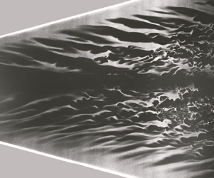
Figures 9 and 10(a) show the Rayleigh scattering flow visualisations on the  $x$–
$x$– $z$ plane of the delta wing at the normal height at $y = 0.5$ mm and 1.0 mm, respectively. Point C in both figures 9 and 10 shows that the cross-flow region is near the leading edge, where the cross-flow streaks can be observed clearly. The angle between the cross-flow streaks and the centreline is about 15 $^\circ$. Downstream of the cross-flow structures, turbulent structures appear (indicated as point T) after the boundary line (green dotted line), which is consistent with the ‘M’-shaped distribution shown in figure 8. Near the centreline at $z = 0$, the transverse pressure gradient makes the fluid converge towards the centreline, resulting in the thickening of the boundary layer. An obvious low-speed streak thus appears there (indicated as point S), which is similar to that observed by Huntley & Smits (Reference Huntley and Smits2000). As $y$ increases to 1.0 mm, prominent high-frequency structures connecting to a cross-flow streak are observed, as shown by point F in figure 10. These structures are composed of a series of small ‘fingers’ extending in the streamwise direction, which is similar to the secondary instability structure of travelling cross-flow vortices observed in low-speed flows (Wassermann & Kloker Reference Wassermann and Kloker2003). Figure 10(b) shows the temperature contours at $y = 1$ mm arising from the DNS simulation. The appearance of travelling cross-flow vortices, as well as the secondary finger-like structures, are also presented in the DNS result. A good agreement has been achieved in the wavelength of travelling cross-flow waves and the secondary structures between the DNS and experiments, which are 12 and 5 mm in the streamwise direction, respectively, corresponding to frequencies of about 50 and 120 kHz. By comparison with the linear stability theory in figure 6, it is seen that these cross-flow and secondary streaks respectively correspond to the travelling cross-flow waves and the second mode. Previous studies have shown that stationary cross-flow vortices dominate transitions in low-disturbance flows (Borg & Kimmel Reference Borg and Kimmel2016; Yates et al. Reference Yates, Matlis, Juliano and Tufts2020), whereas travelling waves dominate in high-disturbance flows. In this study, the wind tunnel runs under noisy conditions with the suction valve closed so that the disturbance level of the coming stream is as high as 1 $\%$, which benefits the growth of travelling cross-flow waves. Moreover, the surface of the model is highly polished so that the stationary cross-flow vortices are depressed. Hence, the travelling cross-flow vortices rather than their stationary counterparts are observed in this study.

Figure 9. Single-pulsed flow visualisations on the  $x$–
$x$– $z$ section of the delta wing at $y = 0.5$ mm. The black area indicates high temperatures and the sublimation of carbon dioxide (>143 K), the white area indicates low temperatures and gaseous carbon dioxide(<143 K) and the black-and-white boundary gives the flow structure characteristics. The green dotted line indicates the boundary where turbulence occurs. C, cross-flow structure; T, turbulent structure; S, centreline streak structure.

Figure 10. (a) Single-pulsed flow visualisations on the  $x$–
$x$– $z$ section of the delta wing at $y = 1$ mm. The black area indicates high temperatures and the sublimation of carbon dioxide (>143 K), the white area indicates low temperatures and gaseous carbon dioxide(<143 K) and the black-and-white boundary gives the flow structure characteristics. (b) DNS temperature contours at $y = 1$ mm. C, cross-flow structure; T, turbulent structure; S, centreline streak structure; F, finger-like secondary structure.
The evolution of the instabilities is then presented in figure 11 in the form of pressure sensor measurement. Figure 11(a) shows the power spectrum of the surface pressure pulsation measured by the PCB sensors. A line with the slope of  $-\frac {5}{3}$, indicating a turbulent state, is also added. Since the low-frequency cutoff frequency of the PCB sensor is 11 kHz, the original signal is filtered with a band of 11–900 kHz before the power spectrum calculation is performed. It can be seen that there are three spectral peaks located at 11–30 kHz, 30–50 kHz and 110–130 kHz, as shown by arrows ‘1’, ‘2’ and ‘3’, respectively. Note that the sensor's frequency response is only flat to about 100 kHz (Schneider Reference Schneider2019), and thus the amplitude distribution presented in figure 11(a) might be distorted from the reality. However, in this study, only the frequency rather than the amplitude information is considered so that the effect of the sensor's response function can be neglected. Figures 11(b)–11(d) show the time series of the pressure pulsation measured by the PCB sensors under different filter bandwidths of 11–30 kHz, 30–50 kHz and 110–130 kHz, respectively. Here, six typical PCB positions are selected for analysis to facilitate the observation. By comparison with the flow visualisation and linear stability theory discussed previously, the instabilities with frequencies 30–50 kHz and 110–130 kHz can be seen to correspond to the travelling cross-flow instability and the second mode, respectively. The instability at 11–30 kHz appears further. Finally, the flow becomes turbulent with the slope approaching $-\frac {5}{3}$.

Figure 11. Wall pressure fluctuations measured by the PCB sensors. (a) The power spectrum of the pressure fluctuation signals measured by the PCB sensors. (b–d) The time series of surface pressure fluctuations with frequency bands of 11–30 kHz, 30–50 kHz and 110–130 kHz, respectively. The PCB positions are from  $x = 232.5$ mm to 377.5 mm with an intervals of 14.5 mm and from $z = 45.1$ mm to 6.5 mm with an interval of $-3.8$ mm. The dashed arrow in the figure indicates the direction of the disturbance evolution.
The high-speed schlieren technique is further used to obtain the global evolution of density gradient disturbances on the delta wing. During a wind tunnel blow, 150 000 images were collected at a frequency of 380 kHz. Different instability modes were then obtained from both the schlieren data and DNS through band-pass filtering at 12–32 kHz, 38–58 kHz and 108–128 kHz and are compared in figure 12. The wave angles of the three modes differ significantly. The low-frequency wave grows with the longest wavelength of the three modes, as shown in figures 12(a) and 12(d). The angle between its wavefront and the  $x$-axis is about $-20^\circ$. The high-frequency instability evolves with the shortest wavelength of the three modes, as shown in figures 12(c) and 12(f). The medium-frequency instability is shown in figures 12(b) and 12(e). It should be emphasised here that only the DNS results show the travelling cross-flow instability structure near the leading edge; the experiments do not because that region is opaque in the model, as shown in figure 1(b).

Figure 12. The transient amplitude distribution of the schlieren intensity with filter bandwidths in the ranges (a,d) 12–32 kHz, (b,e) 38–58 kHz and (c,f) 108–128 kHz. Panels (a–c) arise from experiments and panels (d–f) arise from the DNS. The amplitude is normalised by the maximum value.
The disturbance amplitudes are calculated for each pixel of the schlieren images from the root mean square (RMS) of the time series. Figure 13 shows the amplitude distribution of the different modes on the delta wing. The two red dotted lines indicate the locations of the maximum values of the medium- and high-frequency instabilities along the streamwise direction, which are approximately parallel to the leading edge when  $z > 30$ mm. The medium-frequency instability, the cross-flow instability, grows first and decays along the streamwise direction. The second mode increases significantly downstream. The region where the second mode grows has a similar shape to the region where the cross-flow instability grows, but its location is shifted downstream. The attenuation of the second mode can be observed near the tail of the model, where the low-frequency mode begins to grow. The region where the low-frequency wave grows is triangular, and the growth follows the completion of the transition, as shown by the ‘M’ shape in the IR image (figure 8).

Figure 13. The amplitude distribution filtered from the schlieren images. The filter bandwidths are (a,d) 12–32 kHz, (b,f) 38–58 kHz and (c,g) 108–128 kHz. Panels (a–c) arise from experiments and panels (d–f) arise from DNS. The amplitude is normalised by the maximum value.
4.2. DNS simulation results
To identify these observations in experiments, the DNS flow structures are presented as  $Q$-criterion isosurfaces $(Q=0.02)$ in figure 14(a). The colour map indicates the height to the surface. The structures of the travelling cross-flow vortices (shown by redder colours at higher positions) are clearly displayed (figure 14b), aligned at an inclined angle of about 30 $^\circ$ to the $x$-axis. As shown in figure 14(c), these cross-flow vortices intersect with the bluer structures near the wall. The height of the cross-flow vortices is about 1.0 mm. In figure 10, the laser sheet is at a height of about 1.0 mm, so the flow visualisation clearly captures the cross-flow vortices. The wavelengths of the cross-flow vortices and the bluer structures near the wall are, respectively, 12.5 and 5 mm, corresponding to frequencies of 48 and 118 kHz.

Figure 14. (a) The DNS flow structures shown by isosurfaces of  $Q$-criteria $(Q = 0.02)$ covering the range of $x\in [100, 300]$ mm and $z\in [0, 80]$ mm with the appearance of (b) travelling cross-flow vortices, (c) second mode, (d) secondary vortices and (e) low-frequency hairpin-like structures. The contours stand for the normal height relative to the wall.
To further identify the nature of the disturbance around 118 kHz and the corresponding bluer structures in figure 14(c), the streamwise velocity disturbance profiles are extracted from the DNS data and are depicted in figure 15. The shape function of the second mode is also given by linear stability theory for comparison. Notably, the profile of the instability agrees well with the linear stability theory prediction at  $x = 150$ mm (at a distance of approximately 20 mm from the leading edge), showing that it indeed belongs to the second mode. The reason for this can be attributed to the typical characteristic of the second mode: the presence of large disturbances beneath the sonic line, accompanied by a compression and expansion motion. These compression and expansion motions persist over a long distance, as shown by the agreement between the instability's profile and linear stability theory beneath the sonic line in figures 15(b)–15(d) and the existence of ‘bluer’ structures near the wall in figure 14. Moreover, with an increase in the streamwise location, a new disturbance peak appears at about $y = 2\unicode{x2013}3$ mm, corresponding to the appearance of the secondary finger-like instability, as shown in figures 10 and 14(d). A detailed explanation of these secondary instabilities is presented in the subsequent section. In general, the instability around 118 kHz is equivalent to the ‘bluer’ structures of the second mode near the wall and the resulting secondary vortices in figure 14.

Figure 15. Streamwise velocity disturbance profiles for the instability around 118 kHz filtered from the DNS at  $z = 29$ mm, (a) $x = 150$ mm, (b) $x = 180$ mm, (c) $x = 210$ mm and (d) $x = 250$ mm. These are compared with the shape function of the second mode as predicted by linear stability theory. The black dotted lines represent the sonic line.
The instability filtered in the range 12–32 kHz corresponds to the low-frequency waves appearing at the end of the transition process (figure 14e), which were previously observed by Bountin, Shiplyuk & Sidorenko (Reference Bountin, Shiplyuk and Sidorenko2000) and Li et al. (Reference Li, Fu and Ma2010) in both experiments and numerical simulations. Zhu et al. (Reference Zhu, Zhang, Chen, Yuan, Wu, Chen, Lee and Gad-el Hak2016) first experimentally demonstrated that the fast growth of the second mode can trigger these low-frequency waves through a nonlinear interaction process over a Mach 6 flared cone. Chen et al. (Reference Chen, Zhu and Lee2017a) studied this problem using nonlinear parabolised equation analysis, showing that a phase-locking interaction mechanism first transfers energy from the second mode to low-frequency waves, and then a parametric resonance takes effect. Li, Zhang & Lee (Reference Li, Zhang and Lee2020) also investigated this phenomenon over a Mach 6 flat plate, which is a condition more similar to that used in this study. The low-frequency waves are identified as the vortical first-mode-like waves and can be enhanced by the second mode through a phase-lock interaction. Zhu et al. (Reference Zhu, Zhu, Gu, Lee and Smith2021) recently studied the role of low-frequency waves in the turbulence production process, which is the same as in the low-speed boundary layers, as well as in turbulent stratified shear layers, discussed recently by Jiang et al. (Reference Jiang, Lee, Chen, Smith and Linden2020a,Reference Jiang, Lee, Smith, Chen and Lindenb, Reference Jiang, Gu, Lee, Smith and Linden2021, Reference Jiang, Lefauve, Dalziel and Linden2022). As shown in figure 14, low-frequency waves appear as hairpin-like vortices before the flow is turbulent. The origin of these hairpin-like vortices is shown in figure 16. The secondary vortex first appears where the cross-flow vortex intersects with the second mode in the wall-normal direction, aligned in the mirrored direction of the cross-flow vortex with respect to the  $x$ direction and, hence, forms a short ‘leg’ of a $\varLambda$-like structure. As time goes by, a head of the $\varLambda$-like structure forms, connecting the secondary vortex to the cross-flow vortex. The structures then evolve into an asymmetric hairpin-like vortex, with the cross-flow vortex disappearing and the secondary vortex extending and finally becoming turbulent at $x =280$ mm.

Figure 16. The convection of flow structures from  $x = 215$–280 mm with a time interval of 5 $\mathrm {\mu }$s. The flow structures are shown by their $Q$ criterion isosurfaces $(Q = 0.0025)$ from the DNS results. The contours stand for the normal height relative to the wall.
5. Analysis and discussion
5.1. Instability interaction
Figure 17 shows the amplitude evolution of the three unstable modes along their respective disturbance propagation directions at  $z = 18$ mm, 23 mm, 27 mm, 29 mm and 37 mm. During data processing, we first select a channel where the second mode grows and extract the amplitude evolution of the high-frequency instability along it. Concurrently, we find the low-frequency channel, whose spanwise position is similar to that of the high-frequency channel, and the amplitude evolution of the low-frequency channel is then determined. As the wave angle of the medium-frequency instability (the cross-flow vortices) is very different from that of the high-frequency instability (see figure 17a), its wavefront intersects with the latter when it travels downstream. A selected low-frequency wave packet encounters three to six cross-flow streaks in the process of downstream propagation and development. The red lines in figure 17 represent the amplitude characteristics of the cross-flow wave that meets the second mode at a certain moment along the cross-flow streaks, and the red dotted line represents the amplitude evolution of the cross-flow instability along the $x$-axis. The DNS results at $z = 29$ mm are also presented in figure 17(g) and can be compared with the experimental results in figure 17(e). For the experiments, the locations of the maximum amplitude for the travelling cross-flow instability, the second mode, and the low-frequency wave are respectively $x = 248$ mm, 276 mm and 349 mm. For the DNS, they are $x = 238$ mm, 260 mm and 370 mm, respectively. The difference between the experiment and DNS is between 4 % and 5.7 %.

Figure 17. (a) A sketch of the instabilities’ evolution paths and their interaction. The amplitude evolution of the low-frequency wave, the travelling cross-flow instability, and the second mode at (b)  $z =18$ mm, (c) $z =23$ mm, (d) $z =27$ mm, (e) $z =29$ mm and (f) $z =37$ mm from the schlieren data, which are compared with (g) DNS data for $z = 29$ mm. The solid red line represents the amplitude distribution of the travelling cross-flow instability along the direction of the cross-flow streaks, the dotted red line represents the amplitude envelope of the travelling cross-flow instability, the black line represents the amplitude evolution of the second mode and the green line represents the amplitude evolution of the low-frequency wave.
It can be seen from the amplitude evolution curves in figure 17(b) that, at  $x = 150$ mm and $z = 18$ mm, all three modes have a positive growth rate. The growth rate of the medium-frequency instability is obviously higher than that of the low- and high-frequency instability. The medium-frequency instability increases rapidly at first, reaches its peak at $x = 250$ mm, and then undergoes amplitude attenuation. The amplitude of the high-frequency instability increases significantly in the range $x = 200$–330 mm, reaches its peak value at 330 mm and then decreases. At $x = 300$ mm, the amplitude growth rate of the low-frequency instability increases, showing a trend of rapid growth until, at the tail of the model, its absolute amplitude exceeds those of the other two growing upstream, leading to transition. The three unstable modes reach their maximum values in the following order: the medium-frequency, high-frequency and then low-frequency, and amplitude attenuation occurs in the medium- and high-frequency instabilities, suggesting that there are interactions among the three modes.
Figure 18 presents the normal-distributed time-averaged profiles of  $u$ and $\rho ({{\rm d}u}/{{\rm d} y})$ at different streamwise locations from the DNS. For $x = 150$ mm, the disturbances are small, and thus the profiles agree well with their undisturbed counterparts. For $x = 230$ mm, the travelling cross-flow disturbance grows to a sufficiently large amplitude (figure 17d), a nonlinear effect occurs, and the time-averaged profiles are distorted compared with their undisturbed counterparts. A prominent feature in the $\rho ({{\rm d}u}/{{\rm d} y})$ profile is the appearance of an additional point where ${{\rm d}(\rho ({{\rm d}u}/{{\rm d} y}))}/{{\rm d} y}=0$. This point is called the generalised inflection point, and it is a necessary condition for inviscid instability in a compressible boundary layer (Lees & Lin Reference Lees and Lin1946). It explains why the second mode is enhanced at this location. For $x = 310$ and 340 mm, the profiles approach turbulent boundary layers with increasing momentum and Reynolds stress in the near-wall region. Such profiles help the growth of the first mode (figure 18).

Figure 18. DNS-provided normal-distributed profiles of  $u$ and $\rho ({{\rm d}u}/{{\rm d} y})$ at $z = 29$ mm, (a) $x = 150$ mm, (b) $x = 230$ mm, (c) $x=310$ mm and (d) $x=350$ mm.
Based on a nonlinear critical layer theory developed using a small parameter perturbation and the asymptotic matching method, Wu (Reference Wu2004) proposed a phase-locking mechanism to explain the rapid growth of 3-D disturbances, but their research focused on the fundamental resonance of the same frequency disturbance. Later, Li et al. (Reference Li, Zhang and Lee2020) and Zhang, Li & Lee (Reference Zhang, Li and Lee2020) extended the phase-locked mechanism to the interaction of different frequency disturbances, holding that the phase velocity locking mechanism can explain the interaction between the second mode and the first mode, and the second mode can transfer energy to the first mode through the phase velocity locking mechanism. In addition, the phase difference locking mechanism can explain the interaction between the first mode and the second mode, which causes the first mode to transfer energy to the second mode. Here, we adopt the method that Li et al. (Reference Li, Zhang and Lee2020) and Zhang et al. (Reference Zhang, Li and Lee2020) used to study the interaction between modes in a flat-plate boundary layer to analyse whether interactions exist between the travelling cross-flow mode and the second mode; the second mode and the first mode; and the travelling cross-flow mode and the first mode. We investigate the internal mechanisms of these interactions; therefore, we need to know the correlation between the phase angle and phase velocity of the three unstable modes.
Information on the phase-angle difference between disturbances can be obtained from a fast Fourier transform (FFT) of the schlieren time series. The phase-angle difference can then be obtained using the formula
 \begin{gather} {d} \phi_{f_1-f_2} = \phi (\omega(f_1))-\phi (\omega(f_2)) , \end{gather}
 \begin{gather}\omega(f) = {FFT}(x(t)), \end{gather}
where  ${d} \phi _{f_1-f_2}$ is the phase-angle difference between disturbances of different frequencies $f_1$ and $f_2$, $\phi (\omega )$ represents the phase angles of $\omega$ (which is a complex number) and $\omega (f)$ represents the FFT of the time series $x(t)$.
Figure 19 shows the RMS of the phase difference between the travelling cross-flow waves and the second mode, the second mode and the first mode, and the travelling cross-flow waves and the low-frequency waves. It can be seen that the phase difference between the travelling cross-flow waves and the second mode is relatively constant, and the RMS of the phase difference is about 20 $^\circ$, which is significantly smaller than the RMS of the phase difference between the second mode and the first mode or the cross-flow waves and the low-frequency waves. The RMS of the phase difference between the second mode and the first mode is about 35 $^\circ$, and the RMS of the phase difference between the cross-flow waves and the low-frequency waves is about 40 $^\circ$. In particular, the phase difference between the cross-flow instabilities and the second mode is constant in the flow direction for $x$ from 150 mm to 330 mm, which indicates that there is a phase difference locking mechanism between the two. The amplitude of the cross-flow instability is large in this region; it then increases further and finally decays. The amplitude of the second mode is small at $x = 150$ mm and increases gradually along the streamwise direction. For $x$ from 250 mm to 330 mm, the growth rate of the second mode wave increases rapidly and the amplitude of the cross-flow wave decreases gradually. This shows that the cross-flow instability transfers energy to the second mode through the phase difference locking mechanism. This result is consistent with experimental results in the flat boundary layer (Zhang et al. Reference Zhang, Li and Lee2020), wherein the low-frequency waves are observed to transfer energy to the second mode wave via a similar phase difference locking mechanism. There is no phase difference locking mechanism between the cross-flow instability and the first mode nor between the second mode and the first mode.

Figure 19. The RMS distribution of the phase difference between the low-frequency wave, the second mode and the travelling cross-flow wave from experimental schlieren data.
To gain deeper insights into the phase-locking mechanism, phase analyses of the travelling cross-flow waves and the second mode at  $z = 37$ mm are conducted based on the schlieren data from the DNS, as shown in figure 20. One wave crest of the second mode is traced over time (the green asterisk marker in figure 20a–e). Notably, as the amplitude of the travelling cross-flow waves increases, a gradual augmentation of the second mode is observed. The wave crest of the second mode aligns with the trough of the travelling cross-flow waves (figure 20a,b). Subsequently, a distinct phase shift occurs at approximately $x = 225$ mm (figure 20c). Following this, the amplitude of the travelling cross-flow waves begins to decrease, whereas the second mode undergoes rapid growth. The wave crest of the second mode becomes positioned on the upslope of the travelling cross-flow waves (figure 20d,e). The phase difference between the two modes remains relatively constant. To validate the influence of the travelling cross-flow waves on the growth of the second mode, an additional DNS case with only one frequency disturbance is implemented, which means in (3.10), $A_1$ is set to 0 whereas $A_2$ is kept at 0.5. A comparison between the two cases is shown in figure 20(f). It can be seen that the absence of the initial 48 kHz disturbance leads to subdued growth rates for both the travelling cross-flow waves and second mode. Moreover, no obvious phase shifts or abrupt alterations in the growth rate manifest in the new case, which confirms the effect of the energy transfer from the travelling cross-flow waves to the second mode.

Figure 20. Phase results and amplitude evolution information of the travelling cross-flow waves and the second mode at  $z = 37$ mm from the schlieren data from the DNS. (a,b) The travelling cross-flow waves and the second mode grow at $x = 190$ mm and $x = 210$ mm. (c) Phase shift point at $x = 220$ mm. (d,e) The travelling cross-flow waves attenuate while the second mode grows rapidly at $x = 238$ mm and $x = 264$ mm. The travelling cross-flow waves and the second mode are extracted by the Butterworth filter with the frequency bands of 42–54 kHz and 112–124 kHz, respectively. The dotted blue line represents the amplitude envelope of the travelling cross-flow instability, the dotted red line represents the amplitude envelope of the second mode, and the vertical dotted cyan line and the green asterisk marker represent the wave crest location of the second mode. The thick blue line and thick red line represent the adjacent waveform of the travelling cross-flow instability and the second mode, respectively. The thin black line represents the entire waveform of the two modes.
As discussed previously, the phase-locking mechanism plays an important role in the nonlinear interaction process. The mechanism shows that resonance comes into effect for two waves with a certain amplitude, given that they have the same or similarly close phase speeds, which leads to the rapid growth of oblique waves. To verify whether this is related to the wave interaction in this case, the phase velocities of different modes in the boundary layer are obtained using the high-frequency schlieren method.
In figure 21, the black line represents the phase velocity of the second mode and the green line represents the phase velocity of the low-frequency waves. The phase velocity of the second mode is between 0.9 $U_0$ and $U_0$, and it gradually decreases as the streamwise location increases. The phase velocity of the low-frequency waves is between 0.6 $U_0$ and 0.8 $U_0$; it remains more-or-less constant in the 150–280 mm range of the streamwise position and increases significantly in the range $x = 280$–370 mm, where the low-frequency waves grow rapidly. Looking at trends, the phase velocities of the second mode and the low-frequency waves in the range 280–370 mm have a tendency to draw close to each other. According to phase-locking theory, a similar phase speed may give rise to a more intense interaction between the two modes. The phase speed gap between the two different modes is even narrower at $x = 280$–370 mm, indicating that the low-frequency waves gain energy from the interaction with the second mode. Considering that the amplitude of the second mode is much larger than that of the low-frequency waves, second mode transfers energy to the low-frequency waves through the phase velocity locking mechanism, promoting a rapid increase in the amplitude of the low-frequency waves. This result is consistent with the interaction mechanism experimentally obtained on a flat plate (Li et al. Reference Li, Zhang and Lee2020). The amplitude of the travelling cross-flow wave is 50 % of that of the low-frequency waves for $x$ between 280 and 370 mm.

Figure 21. The phase velocity of the Mack's first mode and second mode at  $z = 18$ mm. The black line represents the phase velocity of the second mode and the green line represents the phase velocity of the first mode. The phase velocities are normalised using the mainstream velocity $U_0$.
In a study of cross-flow transitions at low speed, Reed & Lin (Reference Reed and Lin1987) analysed the interaction between the cross-flow instabilities and the Tollmien–Schlichting wave, and found that the former leads to double exponential growth of the latter. In the hypersonic cross-flow boundary layer, there have been few studies on modal interaction. The interaction mechanism that transfers energy from relatively low-frequency cross-flow instabilities to the high-frequency second mode is the phase difference locking mechanism. The interaction mechanism that transfers energy from the relatively high-frequency second mode to the low-frequency first mode is the phase velocity locking mechanism. This is a generalisation of phase-locking theory that is consistent with the findings of previous studies on the hypersonic boundary layer (Li et al. Reference Li, Zhang and Lee2020; Zhang et al. Reference Zhang, Li and Lee2020).
5.2. Generation of secondary vortices
As discussed previously, the second mode strengthens with the travelling cross-flow vortices as  $x$ increases to 250 mm. We show in the following that the near-wall ‘bluer’ structures aligned in the direction normal to $x$ in figure 14 are created by the second mode.
The evolution of the cross-flow and secondary structures is dynamically captured by ultrafast flow visualisations with a time interval of 10  $\mathrm {\mu }$s, as shown in figure 22. Following the red arrows, one cross-flow vortex moves downstream (figure 22a), and then periodic small structures appear on the vortex (figure 22b). As time passes, each small structure extends in a direction nearly symmetric to the cross-flow vortex in the $x$-axis (figure 22c–h). At first glance, these structures look like a series of $\varLambda$ or cane-like vortices commonly observed in boundary layer transitions. However, these small structures are higher than the primary cross-flow vortex because they are absent at the lower height (figure 9). All these streaks move at a streamwise speed of about $0.85 U_0$.

Figure 22. Eight-pulsed flow visualisations of the delta wing on the x–z plane at  $y = 1$ mm. Among (a–h), the interval between every two frames is 10 $\mathrm {\mu }$s. The flow is from left to right and the shooting area is $x \in (215, 280)$ mm, $z \in (5, 38)$ mm.
Figure 23 further shows Rayleigh scattering flow visualisations on the  $y$–
$y$– $z$ cross-sections of the delta wing. Initially ( $x = 70$ mm), arrow S points to the centreline, which is a low-speed streak structure caused by the convergence of fluids on both sides to the centre. At $x = 150$ mm, there are wavy structures in the cross-flow region. The wavy structures are travelling cross-flow waves with small amplitudes (indicated as point C). At $x = 190$ mm, 230 mm and 270 mm, the amplitude of the travelling cross-flow vortices gradually increases until saturation. Arrows F at $x = 290$ mm, 310 mm and 350 mm point to a new structure rolling in the direction opposite to that of the cross-flow vortex. It will be further discussed in the following section that the structures indicated by F correspond to the finger-like structures shown in figures 10 and 22(a), which are at a higher position than the cross-flow vortices in the surface-normal direction. The formation of the hairpin vortex structure appears at $x = 390$ mm, like a mushroom in the $y$–
$y$– $z$ cross-section, indicated as ‘ ${\rm H}$’. This leads to the completion of the transition.

Figure 23. Flow visualisations at different  $y$–
$y$– $z$ sections of the delta wing. From top to bottom, the flow position moves downstream. C, cross-flow structure; S, centreline streak structure; F, finger-like secondary structure; H, hairpin-like structure.
As introduced in § 1, the second mode can cause a flow to be alternatively compressed and expanded near the wall, which can also be represented by the divergence of the velocity field
 \begin{equation} \theta=\boldsymbol{\nabla}\boldsymbol{{\cdot}}\boldsymbol{u}, \end{equation}
in figure 24(a). The red colour represents expansion ( $\theta >0$) and the blue colour represents compression ( $\theta <0$). Isolines of the $Q$ criterion are also plotted. As shown, the cross-flow vortices are located at medium height in the boundary layer, while the second mode is basically located near the wall. The $Q$ criterion core caused by the second mode is generally located between the expansion and compression regions. In the near-wall region, the expansion region corresponds to an accelerating region, whereas the compression corresponds to a decelerating region. Thus the most accelerated region (MAR) has been produced between the expansion and compression regions in figure 24(b). Considering the no-slip condition at the wall, the MAR intensifies the wall shear there, as seen by the corresponding high $Q$ value (figure 24c).

Figure 24. (a) The dilatation distribution, as well as  $Q$ criterion isolines, in the $x$–
$x$– $y$ plane at $z=38$ mm. (b) The local dilatation distribution around a $Q$ criterion core caused by the second mode and (c) corresponding $z$ vorticity.
As shown in figure 14, the secondary structures appear where the cross-flow vortices encounter the MAR caused by the second mode. The directions of the three structures are briefly sketched in figure 25. Further downstream, secondary finger-like structures appear with the same frequency as the second mode, which is consistent with the observation in figures 10, 14 and 22.

Figure 25. A sketch of the secondary vortices.
We decompose the vorticity vector of the secondary vortices  $\omega _i$ (indicated by the green lines in figure 14b) into $\omega _{ix}$ and $\omega _{iz}$ along the $x$- and $z$-axes, respectively. Obviously, $\omega _{ix}$ has an opposite direction to the cross-flow vortices, whereas $\omega _{iz}$ is in the same direction. We discuss the generation of $\omega _{ix}$ and $\omega _{iz}$ in the $y$–
$y$– $z$ and $x$–
$x$– $y$ planes, respectively, in the following.
Figure 26 shows the dynamic process of a cross-flow vortex travelling across a MAR induced by the second mode in the  $x$–
$x$– $y$ plane at $z= 38$ mm. The structures are shown using the $Q$ criterion values, which are extracted from the DNS calculation. The yellower colour stands for a larger positive $Q$ criterion value and the bluer colour stands for a smaller one. When the cross-flow vortex is upstream of the second-mode-induced most accelerated region (SMAR), the $Q$ value in the core of the former is much larger than that of the latter, as shown in figure 26(a,b). When the cross-flow vortex approaches the SMAR, it becomes weaker and weaker, as shown in figure 26(c). Then, a new vortex, $\omega _{iz}$, appears over the cross-flow vortex, as shown in figure 26(d,e). As the cross-flow vortex departs from the MAR, the induced $\omega _{iz}$ is still present, forming a leg of the comb-teeth-like structure, as shown in figure 14. The rotation of the cross-flow vortex creates a relatively streamwise and anti-streamwise motion, respectively, above and beneath the vortex core. Because the streamwise acceleration caused by the second-mode (SMAR) has an opposite direction to the relative motion beneath the cross-flow vortex, it makes the cross-flow vortex spin down. Correspondingly, the tangential velocity above the cross-flow vortex is decreased so that the shear strength between the freestream and the cross-flow vortex is intensified, as shown by the black arrow in figure 26(g). Consequently, a new vortex, i.e. $\omega _{iz}$, is generated there ( $y = 3.5$ mm in figure 27).

Figure 26. The contours of the  $Q$-criteria in the $x$–
$x$– $y$ plane for (a) $z = 32$ mm, (b) $z = 31$ mm, (c) $z = 30$ mm, (d) $z = 29$ mm, (e) $z = 28$ mm and (f) $z = 27$ mm. Streamwise velocity profiles along white lines at (b) and (d) are plotted as red and green lines, respectively, in (g).

Figure 27. (a)  $x$ vorticity and (b) $Q$ criteria on the $y$–
$y$– $z$ plane at $x=250$ mm.
Figure 27 shows the generation of  $\omega _{ix}$ in the $y$–
$y$– $z$ plane. As shown in figure 27(a), the rotation of the cross-flow vortex (red colour) induces vorticity in the opposite direction (blue colour) above the vortex at $y = 3.5$ mm in the $y$–
$y$– $z$ plane. The negative vorticity naturally generates rotational motion through $\omega _{ix}$, as shown by the positive $Q$ criterion value in figure 27(b).
In recent calculations by Chen et al. (Reference Chen, Dong, Chen, Yuan and Xu2021a), who studied the stationary cross-flow instabilities over a Mach 6 swept wing, these secondary finger-like structures were also observed connecting to the primary stationary cross-flow vortex. Because their frequencies are the same as that of the  $z$-mode secondary instability mechanism predicted by theoretical analysis, they are believed to be caused by the $z$-mode secondary instability. These secondary structures are similar to secondary structures accompanying the travelling cross-flow vortices in low-speed flows (Wassermann & Kloker Reference Wassermann and Kloker2003). An important discovery by Chen et al. (Reference Chen, Dong, Chen, Yuan and Xu2021a) is footprint structures that have the same frequency as the secondary vortices, which are similar to the bluer structures observed near the wall in figure 14. These structures are aligned in a direction nearly normal to the $x$-axis. Following the previous discussion, these structures are possibly caused by the second mode. As shown by simulations in low-speed boundary layers by Wassermann & Kloker (Reference Wassermann and Kloker2003), the $z$-mode secondary instability of travelling cross-flow vortices is an inherent mechanism that does not depend on the second mode. It should be emphasised here that the frequencies of the second mode and the $z$ mode have the same scale as
 \begin{equation} f=\frac{U_e}{2\delta}, \end{equation}
where  $U_e$ and $\delta$ are the edge velocity and thickness of the boundary layer, respectively (Craig & Saric Reference Craig and Saric2016); hence, the $z$-mode is easily triggered by the second mode in hypersonic boundary layers. These secondary vortices can be triggered by the compression–expansion motion caused by the second mode.
6. Conclusion
In this work, a cross-flow transition over a delta wing has been studied in a Mach 6.5 hypersonic wind tunnel using the Rayleigh scattering flow visualisation, high-speed schlieren and fast-response pressure sensors. DNS under the same flow conditions, as well as analysis based on linear stability theory, have been applied to analyse the transition mechanism. The incoming Mach number  ${Ma}$, the total temperature $T_0$, the total pressure $p_0$, the incoming stream velocity $U_0$ and the corresponding unit Reynolds number ${Re}_{{unit}}$ were 6.5, 410 K, 1.06 MPa, 850 m s $^{-1}$ and $1 \times 10^7$ m $^{-1}$, respectively. Three unstable modes were detected with their frequencies centred at 22 kHz, 48 kHz and 118 kHz. By comparing the flow visualisation, schlieren, DNS and linear stability theory results, these modes were identified as the travelling cross-flow instabilities, the second mode and secondary instabilities and the low-frequency first-mode-like waves. Some conclusions were drawn as follows.
(a) The travelling cross-flow vortices first appear in the cross-flow region near the leading edge of the model. As they grow, a new generalised inflection point in the mean profile of the flow emerges, which benefits the growth of the second mode. As the second mode grows to a sufficient amplitude, it triggers a $z$-type secondary instability at the same frequency on the cross-flow vortices, causing a series of secondary ‘finger’ structures connecting with the cross-flow vortex. At the end of the transition, the low-frequency waves are excited by the second mode through a phase speed locking mechanism with their phase speeds approaching each other.
(b) The flow structure characteristics on multiple sections of the delta wing were obtained experimentally, and the ultra-fast flow visualisations were used in the 3-D boundary layer for the first time to obtain the time-resolved evolution process of the cross-flow travelling wave. It was found that the growth rate of the travelling cross-flow mode on the delta wing plays a dominant role in the cross-flow region, whereas the stationary cross-flow mode is not observed.
(c) The second mode introduces a periodic compression–expansion motion at the bottom of the boundary layer, causing the local region between the expansion and compression to be most accelerated. This MAR has the same wavelength and frequency as the second mode and interacts with the travelling cross-flow vortex to promote the secondary instability of the cross-flow vortex. Finger-like vortices then appear on the updraft side of the cross-flow vortex, which have the same and opposite rotation directions to the travelling cross-flow vortex in the streamwise-normal and spanwise-normal planes, respectively.
(d) These secondary vortices convect downstream along the direction nearly parallel to the streamwise direction and then further evolve into low-frequency hairpin-like structures that finally trigger turbulence. The transition is finally triggered by such low-frequency waves with a similar ‘
${\rm M}$’-shaped distribution over the delta wing as for the low-frequency wave amplitude.


In general, these observations shed light on the interaction mechanism and complex flow structure evolution processes in 3-D hypersonic boundary layers. An investigation of transition process over other 3-D models should be a focus for the future.
Funding
This work was supported by the National Natural Science Foundation of China (grant nos. 12072002, 109103010062, 10921202) and National Key Project (GJXM92579).
Declaration of interests
The authors report no conflict of interest.
Appendix A. Data reduction method
Zero-phase digital filtering is used to filter the time series of the original schlieren data, with the filtering frequency bands 12–32 kHz, 38–58 kHz and 108–128 kHz. The function performs zero-phase digital filtering by processing the input data,  $x$, in both the forward and reverse directions. After filtering the data in the forward direction (to get $x_{1}(t)$), filtfilt (a MATLAB command) reverses the filtered sequence and runs it back through the filter again, so that the phase distortion is zero. In this way, the light intensity in the measurement area corresponding to three different frequency modes can be obtained, and the disturbance propagation path of the wave packet structure in each frame can also be observed in the filtered data $x_f$. The amplitude evolution of the disturbance can be obtained by counting the RMS of the light intensity along the propagation path $L$. Davis 10 provided by LaVision was used for the cross-correlation of the filtered images ( $x_f$) to obtain the phase velocity of the disturbances. With the built-in particle image velocimetry (PIV) iteration algorithm of Davis 10, a $128 \times 128$ pixel window was first used for preliminary cross-correlation, and then cross-correlation was performed again using a $24 \times 24$ pixel window to increase the spatial resolution. The overlap was set to 75 % for the window iteration, which gives a spatial resolution of 6 pixels, corresponding to a physical space of 2.4 mm.
 \begin{gather} x_{1}(t)=\sum_{k=0}^{n} b_{k} x(t+k)-\sum_{k=1}^{n} a_{k} x_1(t+k), \end{gather}
 \begin{gather}x_f(t)=\sum_{k=0}^{n} b_{k} x_{1}(t-k)-\sum_{k=1}^{n} a_{k} x_f(t-k), \end{gather}
 \begin{gather}A=\sqrt{\frac{1}{N}\sum_{n=1}^{N} x_f(t_n)^2},\ {\rm along}\ L, \end{gather}
 \begin{gather}\delta s = xcorr_{davis}(x_f), \end{gather}
 \begin{gather}U_c=\delta s/ \delta t, \end{gather}
where  $a_k,b_k$ are coefficients of the filter, $n=5$ represents the order of the filter, $x_f$ is the filtered data, $A$ is the amplitude of disturbances, $N=300$ is the number of sampling images, $\delta s$ represents the displacement between two frames and $\delta t$ represents the time interval between two frames.
Using a Fourier transform of the schlieren time series, phase-angle difference information between different disturbances could be obtained. The phase-angle difference was obtained using the formula:
 \begin{gather} \omega(f,t^{\prime })=\sum_{n=0}^{N-1}x(t^{\prime }+t_n) \,{\rm exp}(-2i{\rm \pi} t_n\,f), \end{gather}
 \begin{gather}{d} \phi_{f_1-f_2}(t^{\prime })={\rm atan} \frac{{\rm imag}(\omega(f_1,t^{\prime }))}{{\rm real}(\omega(f_1,t^{\prime }))}-{\rm atan} \frac{{\rm imag}(\omega(f_2,t^{\prime }))}{{\rm real}(\omega(f_2,t^{\prime }))}-2{\rm \pi} (f_1-f_2)t^{\prime }, \end{gather}
 \begin{gather}{RMS}_{{d} \phi_{f_1-f_2}}=\sqrt{\sum_{m=1}^{M} ({d} \phi_{f_1-f_2}(t^{\prime }_m)-\frac{1}{M}\sum_{m=1}^{M} {d} \phi_{f_1-f_2}(t^{\prime }_m))^2}, \end{gather}
where  $\omega (f,t^{\prime })$ represents a Fourier transform of time series $x(t)$ with the initial time $t^{\prime }$, real and imag represent the real and imaginary parts of a complex number, $N=300$ is the number of sampling points for Fourier transform, ${d} \phi _{f_1-f_2}$ is the phase-angle difference between disturbances of different frequencies $f_1$ and $f_2$, ${RMS}_{{{d} \phi _{f_1-f_2}}}$ is the RMS of the phase-angle difference and $M=500$ is the number of sampling points for the RMS.


 Open access