


1. Introduction
The rise of convolutional neural networks (CNNs) in computer vision has spurred a flurry of applications in fluid mechanics (Brunton, Noack & Koumoutsakos Reference Brunton, Noack and Koumoutsakos2020), where there is natural crossover due to local or global equivariances and the expectation of lower-dimensional dynamics beneath the high-dimensional observations. One example of successful crossover from computer vision to fluid mechanics is ‘super-resolution’ (Dong et al. Reference Dong, Loy, He and Tang2016) where a CNN is trained to generate a realistic high-resolution image from a low-resolution input. This is typically done by showing a neural network many examples of high-resolution snapshots which have been coarse-grained; the network then learns a data-driven interpolation scheme rather than fitting a low-order polynomial (Fukami, Fukagata & Taira Reference Fukami, Fukagata and Taira2019).
CNNs trained to perform super-resolution have demonstrated a remarkable ability to generate plausible turbulent fields from relatively scarce observations (Fukami et al. Reference Fukami, Fukagata and Taira2019; Fukami, Fukagata & Taira Reference Fukami, Fukagata and Taira2021). Recent efforts have focused on accurate reproduction of terms in the governing equation, or on the reproduction of spectral properties of the flow (Fukami, Fukagata & Taira Reference Fukami, Fukagata and Taira2023), which is often attempted with additional terms in the loss function used to train the model. Almost all examples rely on a dataset of high-resolution ground-truth images, with some recent focus on maintaining accuracy in a low-data limit (Fukami & Taira Reference Fukami and Taira2024). One exception to this is the study from Kelshaw, Rigas & Magri (Reference Kelshaw, Rigas and Magri2022) in low-Reynolds-number Kolmogorov flow, where high-resolution images were generated by minimising a loss evaluated on the coarse grids, which includes a small contribution from a term encouraging the solution to satisfy the governing equations at each point on the coarse grid.
This paper introduces a robust super-resolution algorithm for high-Reynolds-number turbulence which does not require high-resolution data, but instead is trained by attempting to match the time-advanced, super-resolved field to a coarse-grained trajectory. A key component in this approach is the use of a fully differentiable flow solver in the training loop, which allows for the time marching of neural network outputs and, hence, the use of trajectories in the loss function. The inclusion of a ‘solver in the loop’ (Um et al. Reference Um, Brand, Fei, Holl, Thuerey, Larochelle, Ranzato, Hadsell, Balcan and Lin2020) when training neural networks has been shown to be a particularly effective way to learn new numerical schemes (Kochkov et al. Reference Kochkov, Smith, Alieva, Wang, Brenner and Hoyer2021) and to learn effective, stable turbulence parameterisations (List, Chen & Thuerey Reference List, Chen and Thuerey2022). With the coarse-grained trajectory comparison used here, the optimisation problem for network training is very similar to variational data assimilation (4DVar; see Foures et al. Reference Foures, Dovetta, Sipp and Schmid2014; Li et al. Reference Li, Zhang, Dong and Abdullah2019; Wang & Zaki Reference Wang and Zaki2021). For 4DVar of three-dimensional (3-D) homogeneous turbulence, a key bottleneck to accurate reconstruction of the smaller scales is the level of coarse-graining, with a consensus emerging on a critical length scale of  $l_C \approx 5{\rm \pi} \eta _K$ (Lalescu, Meneveau & Eyink Reference Lalescu, Meneveau and Eyink2013; Li et al. Reference Li, Zhang, Dong and Abdullah2019), where $\eta _K$ is the Kolmogorov scale (note that in wall-bounded flows there are different criteria involving the Taylor microscale; Wang & Zaki Reference Wang and Zaki2021, Reference Wang and Zaki2022; Zaki Reference Zaki2024). The hope with incorporating a neural network in this optimisation process is that, through exposure to a wide range of time evolutions, the model can learn an efficient parameterisation of the inertial manifold and thus generate plausible initial conditions where 4DVar would be expected to struggle.
2. Flow configuration and neural networks
2.1. Two-dimensional turbulence
The super-resolution approach developed in this paper is applied to monochromatically forced, two-dimensional (2-D) turbulence on the two-torus (Kolmogorov flow). Solutions are obtained by time integration of the out-of-plane vorticity equation,
 \begin{equation} \partial_t \omega + {\boldsymbol u} \boldsymbol{\cdot} \boldsymbol{\nabla} \omega = \frac{1}{Re}\Delta \omega - \alpha \omega - n \cos(n y).\end{equation}
The velocity  ${\boldsymbol u} = (u, v)$ may be obtained from the vorticity via solution of the Poisson problem for the streamfunction $\Delta \psi = -\omega$, where $u = \partial _y \psi$ and $v = -\partial _x\psi$. Equation (2.1) has been non-dimensionalised with a length scale based on the fundamental wavenumber for the box, $1/k^* = L_x^* / 2{\rm \pi}$, and a time scale defined as $(k^* \chi ^*)^{-1/2}$, where $\chi ^*$ is the strength of the forcing per unit mass in the momentum equations. This results in a definition of the Reynolds number $Re:= (\chi ^* / k^{*3})^{1/2} /\nu$. As in previous work (Chandler & Kerswell Reference Chandler and Kerswell2013; Page, Brenner & Kerswell Reference Page, Brenner and Kerswell2021; Page et al. Reference Page, Norgaard, Brenner and Kerswell2024) the number of forcing waves is set at $n=4$, while the box has unit aspect ratio such that its size is $L_x = L_y = 2{\rm \pi}$ in dimensionless units.
Two Reynolds numbers are considered in this work,  $Re= 100$ and $Re=1000$. For the latter, a linear damping term is included in (2.1) with coefficient
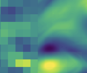
  $\alpha =0.1$ to prevent the build up of energy in the largest scales. Representative snapshots of the vorticity at both Reynolds numbers are reported in figure 1, where the Taylor microscale is also indicated as well as the ‘critical’ length scale for assimilation $l_C := 5{\rm \pi} \eta _K$. Note that while the latter scale has been observed to be critical in 3-D flows, the scales for synchronisation in two dimensions will differ due to the dual cascades. However, we find that these scales still provide a good characterisation of where assimilation struggles in this configuration. Equation (2.1) is solved using the fully differentiable JAX-CFD solver (Kochkov et al. Reference Kochkov, Smith, Alieva, Wang, Brenner and Hoyer2021). The pseudospectral version (Dresdner et al. Reference Dresdner, Kochkov, Norgaard, Zepeda-Núñez, Smith, Brenner and Hoyer2023) of this solver is used here, with resolution $N_x \times N_y = 128\times 128$ at $Re=100$ and $N_x \times N_y = 512 \times 512$ at $Re=1000$.
Snapshots of spanwise vorticity from example trajectories at  $Re=100$ ((a), contours run between ${\pm }10$) and $Re=1000$ ((b), contours run between ${\pm }15$). The black grids in the leftmost panels highlight coarse-graining by a factor of 16 (thin lines) or 32 (thick lines) relative to the simulation resolution. The Taylor microscale (relative to the length scale $L_x^* / (2{\rm \pi} )$) is indicated by the labelled vertical red lines, while the blue line measures $5{\rm \pi} \eta _K$.

2.2. Super-resolution problem and neural network architecture
The objective of super-resolution is to take a coarse-grained flow field, here a velocity snapshot, and interpolate it to a high-resolution grid. The coarse-graining operation considered here, denoted  $\mathcal {C}: \mathbb {R}^{N_x\times N_y\times 2} \to \mathbb {R}^{N_x/M \times N_y/M\times 2}$, is defined by sampling the original high-resolution data at every $M > 1$ gridpoint in both $x$ and $y$, motivated by observations that may be available in an experiment with sparse sensors. There is nothing in the approach outlined in the following that is reliant on a particular form of the operator $\mathcal {C}$ (for example, average pooling or a Gaussian filter might be used instead). A function $\mathcal {N}: \mathbb {R}^{N_x/M \times N_y/M\times 2} \to \mathbb {R}^{N_x\times N_y\times 2}$ is then sought which takes a coarse-grained turbulent snapshot $\mathcal {C}({\boldsymbol u})$ and attempts to reconstruct the high-resolution image. The function $\mathcal {N}$ is defined by a CNN (LeCun et al. Reference LeCun, Bottou, Bengio and Haffner1998) described in the following, and is found via minimisation of a loss function. In ‘standard’ super-resolution (Fukami et al. Reference Fukami, Fukagata and Taira2019, Reference Fukami, Fukagata and Taira2021) this loss usually takes the form
 \begin{equation} \mathscr L_{SR} = \frac{1}{N_S }\sum_{j=1}^{N_S}\| {\boldsymbol u}_j - \mathcal{N}_{\boldsymbol \varTheta} \circ \mathcal{C} ( {\boldsymbol u}_j) \|^2,\end{equation}
where  $N_S$ is the number of snapshots in the training set and $\boldsymbol {\varTheta }$ are the weights defining the neural network. Note that in this work only reconstruction of velocity is used, due to challenges in estimating vorticity from coarse-grained experimental data. Models trained on vorticity outperform the velocity networks in a variety of ways, particularly in reproduction of the spectral content (not shown).
Various approaches have added additional terms to (2.2) to encourage the output to be more physically realistic (e.g. solenoidal, prediction of specific terms in the governing equation; see Fukami et al. Reference Fukami, Fukagata and Taira2023). In this work incompressibility is built into the network architecture (see the following), while the loss considered here does include additional physics but this is done using trajectories obtained from time marching (2.1):
 \begin{equation} \mathscr L_{TF} = \frac{1}{N_S N_T}\sum_{j=1}^{N_S}\sum_{k=1}^{N_t}\| \boldsymbol \varphi_{t_k}({\boldsymbol u}_j) - \boldsymbol \varphi_{t_k}\circ \mathcal{N}_{\boldsymbol \varTheta} \circ \mathcal{C} ( {\boldsymbol u}_j) \|^2, \end{equation}
where  $\boldsymbol {\varphi }_t$ is the time-forward map (with conversion from velocity to vorticity and back) of (2.1), and $t_k \in \{0, \Delta t, \ldots (N_t -1)\Delta t\}$ with $\Delta t = M \delta t$, where $\delta t$ is a simulation timestep. The unroll time, $T=(N_t - 1)\Delta t$, and coarsening factor $M$ are design choices. Here the temporal coarsening is set to match the coarsening in space, $M\equiv 2^n$, with either $n\in \{4, 5\}$. The selection of the unroll time is constrained by the Lyapunov time for the system. In this work $T=1.5$ at $Re=100$, while results will be shown at both $T\in \{0.5, 1\}$ at $Re=1000$. These choices were guided by the performance of data assimilation at the finer value of $M=16$, shown alongside the super-resolution results in § 3, where reconstruction errors after an unroll time are $O(2\,\%)$ at $Re=100$ and $O(1\,\%)$ at $Re=1000$ (with $T=1$). Training a neural network with a loss like (2.3) requires backpropagation of derivatives with respect to parameters through the time-forward map. This is accomplished here through use of the fully differentiable flow solver JAX-CFD which was created for this purpose (Kochkov et al. Reference Kochkov, Smith, Alieva, Wang, Brenner and Hoyer2021; Dresdner et al. Reference Dresdner, Kochkov, Norgaard, Zepeda-Núñez, Smith, Brenner and Hoyer2023).
While (2.3) incorporates time evolution, it still requires access to high-resolution reference trajectories. An alternative loss, inspired by data assimilation, can be defined based only on coarse observations,
 \begin{equation} \mathscr L_{TC} = \frac{1}{N_S N_T}\sum_{j=1}^{N_S}\sum_{k=1}^{N_t}\| \underbrace{\mathcal{C} \circ \boldsymbol\varphi_{t_k}({\boldsymbol u}_j)}_{(i)} - \underbrace{\mathcal{C} \circ \boldsymbol\varphi_{t_k}\circ \mathcal{N}_{\boldsymbol \varTheta} \circ \mathcal{C} ( {\boldsymbol u}_j)}_{(ii)} \|^2.\end{equation}
The highlighted terms represent: (i) a coarse-grained trajectory, accomplished here by coarse-graining the output of the flow solver, but conceptually this could also be a set of experimental measurements at a set of sequential times; and (ii) the forward trajectory of the super-resolved prediction, which is then coarse-grained for comparison with (i).
While in this work the solver is used to unroll the reference data in term (i) of (2.4) (and the corresponding term in (2.3)), there is no need for a solver here in the general case: (i) represents training data. The solver is always required in the second term (ii), however, where it is used to advance the high-resolution prediction of the network. Note that while unrolling in time is used in the loss to train the model, the neural network  $\mathcal {N}_{\boldsymbol {\varTheta }}$ must produce a high-resolution field from a single coarse-grained snapshot, $\mathcal {C}({\boldsymbol u})$. Thus, at runtime the approach differs substantially from variational data assimilation, which performs a trajectory-specific optimisation.
The neural networks used in this study are purely convolutional with a residual network (‘ResNet’) structure (He et al. Reference He, Zhang, Ren and Sun2016). If the coarsening reduces the dimension of the input by a factor of  $2^n$, then $n$ residual layers with upsampling by a factor of 2 are used to reconstruct the high-resolution field. The output of the $n$ residual convolutions is a field, $\tilde {{\boldsymbol u}}'$, with the correct dimensionality (resolution $N_x \times N_y$ and two channels for $u$ and $v$). However, $\tilde {{\boldsymbol u}}'$ does not by default satisfy the divergence-free constraint. Rather than add a soft constraint to the loss, an additional layer is included in the neural network which performs a Leray projection to produce the divergence free-prediction for the high-resolution velocity, $\mathscr P(\tilde {{\boldsymbol u}}') = \tilde {{\boldsymbol u}}' - \boldsymbol {\nabla } \varDelta ^{-1} \boldsymbol {\nabla } \boldsymbol {\cdot } \tilde {{\boldsymbol u}}'$. This operation is defined as a custom layer within a Keras neural network (Chollet Reference Chollet2015), and is performed in Fourier space where inversion of the Laplacian is trivial (full source code is provided in the repository https://github.com/JacobSRPage/super-res-dynamical, while weights for all neural networks presented here are available at https://doi.org/10.7488/ds/7858). Without the Leray layer, the predictions of the model typically feature a non-solenoidal component in the highest wavenumbers, which is removed in a single timestep of the solver. The inclusion of the Leray layer does not have a noticeable effect on model performance, but ensures that the initial conditions satisfies the physical constraint $\boldsymbol {\nabla } \boldsymbol {{{\cdot }}} {\boldsymbol u} =0$.
The full architecture is sketched in figure 2. A fixed number of 32 filters is used at each convolution, apart from the final layers where only 2 channels are required for the velocity components. The kernel size is fixed at  $4\times 4$ across the network and periodic padding is used in all convolutions throughout the network so that the periodic boundary conditions in the physical problem are retained when upsampling. In this work downsampling is performed by a factor of either $16$ or $32$, which results in a total number of trainable parameters of either $N_{16}\sim 1.33 \times 10^5$ or $N_{32}\sim 1.67 \times 10^5$, respectively. While some experimentation was performed with varying the kernel size through the network, the architecture has not been heavily optimised and more complex configurations may be more effective. Either GeLU (Hendrycks & Gimpel Reference Hendrycks and Gimpel2016) or linear (no) activation functions are used between layers, as indicated in figure 2.

The models examined in § 3.1 were trained on datasets of  $N_{long} = 60$ trajectories at each $Re$. Each trajectory is of length $T_{long} = 100$ and is sampled every $\Delta T_{long}=2$ to generate $N_s=50$ initial conditions for $N_{long} \times N_s=3000$ short trajectories of length $T$ for use in the dynamic loss functions ((2.3) and (2.4)). Data augmentation of random shift reflects and rotations was applied during training. Networks were all trained using an Adam optimiser (Kingma & Ba Reference Kingma and Ba2015) with a learning rate of $\eta = 10^{-4}$ and a batch size of 16 for 50 epochs, where the model with best-performing validation loss (evaluated on 10 % of data partitioned off from the training set) was saved for analysis. In addition, models were also trained on a much smaller dataset of 500 short (length $T$) trajectories. These trajectories were contaminated with noise and serve to both (i) investigate the low-data limit and (ii) the robustness of the algorithm to noisy measurements. These results are reported in § 3.2. All results are reported on separate test datasets generated in the same manner as the training data.
Note that the rather large downsampling factors used in the models result in a set of coarse-grained observations which are either spaced roughly a Taylor microscale,  $\lambda _T$, apart ( $M=16$) or spaced further than the microscale ( $M=32$). As a result, ‘standard’ data-assimilation strategies struggle at both resolutions, which is discussed further in the following. The coarsened grids, $\lambda _T$ and $l_C$, were all included earlier in figure 1 for comparison.
3. Super-resolution with dynamics
3.1. Large dataset results
The performance of the ‘dynamic’ loss functions ((2.3) and (2.4)), with training on the larger datasets described above, is now assessed. The test average (and standard deviation) of the snapshot reconstruction error,
 \begin{equation} \varepsilon_j(t) = \frac{\| \boldsymbol{\varphi}_t({\boldsymbol u}_j) - \boldsymbol \varphi_t \circ \mathcal{N}_{\boldsymbol{\varTheta}} \circ \mathcal{C}({\boldsymbol u}_j)\|}{\| \boldsymbol{\varphi}_t({\boldsymbol u}_j)\|},\end{equation}
is reported both at  $t=0$ and $t=T$ for all models in figure 3. The unroll time $T=1.5$ for all results at $Re=100$, while at $Re=1000$ two values are used; $T=0.5$ when $M=16$ and $T=1$ when $M=32$. Other models were trained with various similar $T$-values (not shown) and those presented here were found to be the best performing.
Summary of network performance at both  $Re=100$ and $Re=1000$. (a) Average test-set errors (symbols; lines show $\pm$ a standard deviation). Models trained using ‘standard’ super-resolution loss (2.2) are shown in green, time-advancement loss on the high-resolution grid (2.3) is shown in blue and the coarse-only time-dependent loss (2.4) is shown in red. (b) As (a) but errors are now computed after advancing ground truth and predictions forward in time by $T$. (c) Example model performance for a single snapshot at both $Re$ and coarsening factors. Streamwise velocity is shown with contours running between ${\pm }3$. The output of models trained with losses (2.3) and (2.4) is shown.

Figure 3 includes results obtained with standard super-resolution (loss function (2.2)) along with both dynamic loss functions ((2.3) and (2.4)). When high-resolution data are available, the average errors in figure 3 indicate that including time evolution in the loss (2.3) does not have a significant effect on reconstruction accuracy relative to the ‘standard’ super-resolution approach in most cases. The error after the model outputs have been unrolled by  $T$ is comparable to that at initial time for all coarsenings and $Re$ values.
The  $Re=100$ results are noticeably worse than those at $Re=1000$. This is perhaps unsurprising given that coarse-graining at the lower $Re$ value, particularly at $M=32$, means that observations are available on a scale which is larger than typical vortical structures and much larger than the ‘critical’ length $l_C$; see figures 1 and 3(c). In contrast, the $M=32$ coarsening at $Re=1000$ is not as significant relative to $l_C$, though the spacing is still larger than this value.
Most interestingly, the performance of the models trained without high-resolution data (loss function (2.4), red symbols in figure 3), is also strong. The reconstruction errors at initial time  $t=0$ are comparable to those obtained with high-resolution models, e.g. at $Re=1000$ the $M=32$ error is ${\sim }1.5 \times$ that from the high-resolution models. A visual inspection of the reconstruction shows faithful reproduction of the larger scale features in the flow. Examples of this behaviour are included in figure 3(c), where it is challenging to distinguish the differences by eye between the coarse and fine models at $Re=1000$. The reconstruction errors decrease as the predictions from the coarse models are marched forward in time and at $t=T$ are near-identical to, and sometimes lower than, those obtained via the high-resolution approaches.
The drop in  $\varepsilon (T)$ relative to $\varepsilon (0)$ for the coarse-grained-only approach at $Re=1000$ mimics observations of variational data assimilation in turbulent flows (Li et al. Reference Li, Zhang, Dong and Abdullah2019; Wang & Zaki Reference Wang and Zaki2021). Data assimilation is also considered here as a point of comparison for the performance of models trained only on coarse observations. Given coarse-grained observations of a ground truth trajectory $\{\mathcal {C} \circ \boldsymbol {\varphi }_{t_k}({\boldsymbol u}_0)\}_{k=0}^{N_T-1}$, an initial condition $\boldsymbol v_0$ is sought to minimise the following loss function:
 \begin{equation} \mathscr L_{DA}(\boldsymbol v_0) := \frac{1}{N_T}\sum_{k=1}^{N_T} \| \mathcal{C} \circ {\boldsymbol\varphi_{t_k}({\boldsymbol u}_0)} - \mathcal{C} \circ \boldsymbol\varphi_{t_k}(\boldsymbol v_0) \|^2.\end{equation}
Equation (3.2) is minimised here using an Adam optimiser (Kingma & Ba Reference Kingma and Ba2015) in an approach similar to the training of neural networks outlined previously. Gradients are evaluated automatically using the differentiability of the underlying solver rather than by construction of an adjoint system. Since data assimilation is performed on velocity (rather than the vorticity), gradients are projected onto a divergence-free solution prior to updating the initial condition. An initial learning rate of  $\eta =0.2$ is used throughout and the number of iterations is fixed at $N_{it}=50$. The initial condition for the optimiser is the coarse-grained field $\mathcal {C}({\boldsymbol u}_0)$ interpolated to the high-resolution grid with bicubic interpolation (note that reconstruction of a high-resolution field directly via simple bicubic interpolation leads to large errors, e.g. $\varepsilon \gtrsim 0.3$ at $M=16$, both in the initial condition and under time evolution).
Example evolutions of the reconstruction error at  $Re = 1000$ and both $M\in \{16, 32\}$ are reported in figure 4 for networks trained with all loss functions ((2.2)–(2.4)), as well as for the data assimilation described above. The data assimilation was performed on equispaced snapshots separated by $M\delta t$ in time within the grey box labelled $T_{DA}$, before the prediction is then unrolled to $T=2.5$. The neural networks, on the other hand, were trained on separate data as described in § 2 with the various loss functions ((2.2)–(2.4)) The grey boxes labelled $T_{SR}$ in figure 4 highlight the unroll time used to train the networks with dynamic loss functions, but the network predicts the high resolution field $\mathcal {N}_{\boldsymbol {\varTheta }}\circ \mathcal {C}({\boldsymbol u})$ from a single snapshot at $t=0$, which is then marched in time. As expected based on the statistics in figure 3, the error between the coarse-only neural network and the ground truth drops rapidly when time marching, becoming nearly indistinguishable from models trained on high-resolution data.
Comparison of model predictions under time advancement at  $Re=1000$ to variational data assimilation for example evolutions at both $M=16$ (a) and $M=32$ (b). Black lines are the time-evolved predictions from data assimilation, red lines the performance of ‘standard’ super-resolution, while blue lines show the performance of the time-dependent loss functions ((2.3) and (2.4)). Solid blue is the coarse-only version, and the symbols identify times where the fields are visualised in figures 5 and 6. Grey regions highlight the assimilation window, where $T_{DA}=1$, and the unroll times to train the networks, $T=0.5$ at $M=16$ and $T=1$ at $M=32$.

Evolution of the out-of-plane vorticity at  $Re=1000$, above the evolution of the reconstructed field from data assimilation and using the coarse-only super-resolution model (coarse-graining here is $M=16$). Note the snapshots correspond to the trajectory reported in figure 4 and are extracted at the times indicated by the symbols in that figure. Contours run between ${\pm }15$. For $t\in \{0, 0.1\}$, a low-pass-filtered vorticity has been overlayed in red/blue lines to show the reproduction of the larger-scale features which would otherwise be masked with small-scale noise. The cutoff wavenumber for the filter matches the coarse-graining and the contours are spaced by $\Delta \omega = 3$.

Evolution of streamwise velocity at  $Re=1000$, above the evolution of the reconstructed field from data assimilation and using the coarse-only super-resolution model (coarse-graining here is $M=32$). Note the snapshots correspond to the trajectory reported in figure 4 and are extracted at the times indicated by the symbols in that figure. Contour levels run between ${\pm }3$.

Notably, the neural networks outperform data assimilation as state estimation for the initial condition. This is most significant at  $M=32$ where the reconstruction error from assimilation is $>40\,\%$ (the coarse-graining at $M=32$ means observations are spaced farther apart than the critical length $l_C$ and assimilation is expected to struggle; see Lalescu et al. Reference Lalescu, Meneveau and Eyink2013; Li et al. Reference Li, Zhang, Dong and Abdullah2019; Wang & Zaki Reference Wang and Zaki2021). At first glance, this is somewhat surprising since the assimilation is performed over the time windows highlighted in grey in figure 4, i.e. for this specific trajectory, while the neural network must make an estimation based only on a single coarse-grained snapshot from the unseen test dataset. Presumably, the improved performance is a result of the model seeing a large number of coarse-grained evolutions during training and hence building a plausible representation of the solution manifold, while each data-assimilation computation is independent. The assimilated field does lead to better reconstruction at later times and at $M=16$ remains close to ground truth beyond the assimilation window, though on average the super-resolution approach is more accurate for $t < T_{DA}$. The super-resolved field from the coarse-only network has a similar time evolution to the standard super-resolution approaches.
A comparison of the time evolution of vorticity for the  $M=16$ coarse-only model and the output of the data-assimilation optimisation is reported in figure 5. In both approaches the initial vorticity is contaminated with high-wavenumber noise, though the low-wavenumber reconstruction is relatively robust (see additional line contours at early times in figure 5). For the neural network output, these small-scale errors quickly diffuse away and the vorticity closely matches the reference calculation by $t\sim 0.25$ (half of the unroll training time). In contrast, the assimilated field retains high-wavenumber error for much longer (it is still noticeable in the vorticity snapshot at $t=1$), although the large-scale structures are maintained on the whole.
These trends are exaggerated at the coarser value of  $M=32$, as shown in $u$-evolution reported in figure 6. Again, the coarse-only neural network faithfully reproduces the larger-scale structures in the flow, with agreement in the smaller scales emerging under time marching. In contrast, the assimilated field remains contaminated by higher-wavenumber noise throughout the early evolution. These differences in spectral content are examined in figure 7: both the super-resolved and assimilated fields reconstruct the low-wavenumber amplitudes before the Nyquist cutoff $k_N$, with the super-resolved field falling away more rapidly leading to relatively flat spectral content just beyond $k_N$ (resulting in under- and then over-prediction of the spectral content in the true field). The assimilated field matches the scaling of the direct cascade (here ${\sim }k^{-4}$) over a slightly wider range of scales than the network prediction, but with significant energy in the small scales. In contrast, the super-resolved field has much lower-amplitude small-scale noise; the spectrum rapidly adjusts to match ground truth under time evolution (see figure 7b).
Energy spectra for coarse-grained network and assimilated fields. (a) Energy in the initial condition for evolution in figure 6 (grey), energy spectrum for the assimilated field (black) and super-resolved field (from coarse observations only, blue). (b) Energy spectra in the time-advanced super-resolved field (blue) at times indicated in figure 6 up to and including  $t = 1$. Time-averaged energy spectrum of the true evolution is shown with the grey dashed line. Vertical lines indicate the forcing wavenumber $k_f=4$ and the Nyquist cutoff wavenumber associated with the filter. Red lines show the scaling $E(k) \propto k^{-4}$.

3.2. Small dataset results with and without noise
The effect of noise on the training (and test) data is now considered briefly as a test of the robustness of the algorithm presented previously. The model architecture and training approach described in § 2 is identical to that discussed before, though models are trained on a smaller dataset of 500 short trajectories of length  $T=1$, with results here reported on a test dataset of 50 trajectories of this length. All results are obtained at $Re=1000$, with coarsening of $M=32$, using the ‘coarse-data-only’ loss function (2.4).
During training noise is added to the reference trajectories in the loss in the following manner (see a similar approach in Wang & Zaki Reference Wang and Zaki2021):
 \begin{equation} \boldsymbol{\varphi}_{t_k}({\boldsymbol u}_j) \to \boldsymbol{\varphi}_{t_k}({\boldsymbol u}_j) + \boldsymbol \eta_{j}(t_k), \end{equation}
where the noisy contribution to the velocity is normally distributed based on the local absolute velocity  $\eta _j(\boldsymbol x, t_k) \sim N(0, \sigma |{\varphi }_{t_k}(u_j)(\boldsymbol x)|)$ (streamwise component shown for illustration). Noise amplitudes of $\sigma \in \{0, 0.05, 0.1\}$ are considered, and noise of the same form is also added to the coarse-grained velocity field which is the input to the neural network.
Summary statistics for all three new models are reported in figure 8, where the test dataset has been contaminated with noise of varying levels. Notably, the noise-less results on the small dataset are comparable to the much larger training set considered in § 3.1, with a roughly  ${\sim }4\,\%$ increase in relative error at both $t=0$ and $t=T$. Figure 8 indicates that the algorithm is robust to low-amplitude noise (both in the training and test data), with performance at the lower value $\sigma = 0.05$ being indistinguishable from the network trained on uncorrupted data. While the stronger $\sigma =0.1$ noise leads to poor reconstruction at $t=0$, all models improve after the unroll time $t=T$. These are promising results in the context of training on experimental data.
Effect of noise on network performance. Mean reconstruction errors (3.1) at  $t=0$ (a) and $t=T$ (b) for networks trained on corrupted data with $\sigma =0$ (blue), $\sigma =0.05$ (green) and $\sigma =0.1$ (red); vertical lines show $\pm$ one standard deviation. The test dataset is contaminated with noise of varying levels, $\sigma \in \{0, 0.05, 0.1\}$, as indicated on the $x$-axes (blue/red data have been offset horizontally slightly to aid visualisation).

4. Conclusions
In this paper an approach to super-resolution has been presented which is similar in spirit to variational data assimilation: the models are trained by requiring that the output of the network can be marched in time while remaining close to the target trajectory. One consequence of this training procedure is that robust models can be trained without seeing high-resolution data: they are trained to match the evolution of the coarse observations only. The resulting models perform comparably to networks trained with high-resolution data, and perform robustly in comparison with data assimilation for state estimation.
The focus in this study has been on periodic, 2-D flow, but there is nothing fundamental in the training loop that restricts the method to this simple configuration. Extension to 3-D problems with walls would require (1) a differentiable flow solver capable of handling other boundary conditions and (2) minor modification of the convolutional architecture (e.g. Dirichlet boundary conditions would naturally imply zero-padding in a convolutional layer). More complex geometries, or the flow past bodies, would necessitate alternative network architectures, though the training approach would remain the same. One thing to bear in mind is the increased cost of the training for 3-D problems: while the network is small and can be trained without a dedicated GPU if only the ‘standard’ super-resolution loss (2.2) is used, the time-dependent versions rely on Navier–Stokes simulations and back-propagation of derivatives through trajectories. Training is equivalent to performing many data assimilations in parallel over minibatches: for context 50 epochs on the large dataset here with a batch size of 16 is equivalent to  ${\sim }9000$ assimilations (training rate is roughly an epoch/hour on an 80 GB A100) though at test time a single call to the network is required in place of assimilation. High-Reynolds-number problems may therefore need to exploit scale invariance of particular flow structures to facilitate transfer learning from smaller-scale flows (see, e.g. Fukami & Taira Reference Fukami and Taira2024).
The outlook is therefore promising for the problem of state estimation in situations where only coarse observations are available, though a key bottleneck is clearly a reliance on a large amount of training data. Exploring the low-data limit, which was touched on in § 3.2, is an important next step. There may also be scope to use the super-resolution predictions to better initialise ‘standard’ 4DVar: this has already shown promise with a learned inverse operator trained on high-resolution data (Frerix et al. Reference Frerix, Kochkov, Smith, Cremers, Brenner, Hoyer, Meila and Zhang2021). Finally, the training procedure on coarse-only observations could be modified to try and improve the spectral content of the initial conditions. This should be relatively straightforward to address in the loss function, for example by weighting early snapshots in the sequence more strongly (such a strategy has been shown to improve the high-wavenumber errors in 4DVar; see Wang, Wang & Zaki Reference Wang, Wang and Zaki2019).
Funding
Support from UKRI Frontier Guarantee Grant EP/Y004094/1 is gratefully acknowledged, as is support from the Edinburgh International Data Facility (EIDF) and the Data-Driven Innovation Programme at the University of Edinburgh.
Declaration of interest
The author reports no conflict of interest.


 Open access