


1. Introduction
Boundary layer tripping is an important part of model-scale studies, where the trip causes transition to turbulence of a boundary layer that would otherwise have remained laminar or transitional, and therefore been less representative of the boundary layers likely to be seen at full-scale Reynolds numbers. This issue is even more important in the context of pressure gradients where favourable pressure gradients cause the boundary layer to thin and resist transition, while adverse pressure gradients have the opposite effect. Consider, for example, a body of revolution at angle of attack where it is impractical to redesign the trip for each angle of attack studied. A trip that is suitable at low Reynolds number, meaning that it yields a turbulent boundary layer without imposing itself in the outer layer, might over-trip the flow at higher Reynolds number where the boundary layer is thinner. Trip location and trip geometry are known to affect the evolution of skin-friction coefficient (Huber & Mueller Reference Huber and Mueller1987; Chesnakas & Simpson Reference Chesnakas and Simpson1996). The choice of trip geometry and location can be challenging since different trip geometries can trigger different modes of perturbations that translate into different evolutions of the boundary layer to a turbulent state. Understanding the trip effects on the transition process is therefore important.
Isolated three-dimensional (3-D) roughness elements immersed in a boundary layer over a flat plate can be considered as a foundational model in this regard. The effects of isolated roughness on transition have been investigated experimentally by Gregory & Walker (Reference Gregory and Walker1956). The main flow pattern is observed to be horseshoe vortices that wrap around the roughness element, and whose legs trail downstream and give birth to the streamwise vortices farther downstream. Baker (Reference Baker1979) has studied experimentally the vortex system around an isolated cylindrical roughness element, and shown the dependency of the horseshoe system dynamics on  $Re_D=U_eD/\nu$ and
  $D/\delta ^{*}$ (where
  $U_e$ is the boundary layer edge velocity,
  $D$ is the cylinder diameter,
  $\nu$ is the kinetic viscosity of the fluid, and
  $\delta ^{*}$ is the displacement boundary layer thickness). The streamwise vortices induced by the 3-D roughness elements create longitudinal streaks downstream that are lifted upwards (Landahl Reference Landahl1980; Reshotko Reference Reshotko2001). The stability properties of the streamwise streaks play important roles in the trip-induced transition. The streamwise longitudinal streaks are related to disturbance transient growth, which can cause transition downstream of the roughness (Fransson et al. Reference Fransson, Brandt, Talamelli and Cossu2004, Reference Fransson, Brandt, Talamelli and Cossu2005). The concept of optimal perturbation was introduced by Böberg & Brösa (Reference Böberg and Brösa1988) and Butler & Farrell (Reference Butler and Farrell1992) to define these ‘most dangerous’ initial perturbations that generate the maximum energy growth. Luchini (Reference Luchini2000) provided a numerical method to determine the optimal perturbation and explain that the linear growth of initially small disturbances can excite nonlinear interactions and cause transition.
Both symmetric (termed ‘varicose’) and anti-symmetric (termed ‘sinuous’) streak instabilities have been detected and are of importance in transitional and turbulent boundary layers. The varicose type is associated with horseshoe vortices that originate from a normal inflectional instability in the streamwise velocity profile (Robinson Reference Robinson1991; Asai, Minagawa & Nishioka Reference Asai, Minagawa and Nishioka2002; Skote, Haritonidis & Henningson Reference Skote, Haritonidis and Henningson2002). The sinuous streak instability is associated with a base state with a spanwise inflection and contributes to the regeneration of near-wall turbulence (Jiménez & Moin Reference Jiménez and Moin1991; Skote et al. Reference Skote, Haritonidis and Henningson2002). Local stability analysis has been used to investigate the streamwise streaks past a single roughness element (Piot, Casalis & Rist Reference Piot, Casalis and Rist2008; Shin, Rist & Krämer Reference Shin, Rist and Krämer2015). Asai et al. (Reference Asai, Minagawa and Nishioka2002) observed that wider streaks more easily undergo varicose breakdown while narrower streaks are more likely to undergo the sinuous breakdown. De Tullio et al. (Reference De Tullio, Paredes, Sandham and Theofilis2013) conducted bi-global stability analysis to investigate transition induced by a sharp-edged isolated roughness element in a supersonic boundary layer, and suggest that the varicose mode is associated with the entire 3-D shear layer while the sinuous mode is a consequence of the lateral streaks. While local stability analysis can reconstruct both direct and adjoint modes at low computational cost, the results are less accurate when the flow is less parallel (Juniper & Pier Reference Juniper and Pier2015). Siconolfi et al. (Reference Siconolfi, Citro, Giannetti, Camarri and Luchini2017) proposed a correction to local stability analysis to improve the prediction of the globally unstable modes.
With large-scale linear algebra computations being possible, global linear stability theory (Theofilis Reference Theofilis2011) may be performed and is useful for non-parallel flows such as roughness wakes, and is therefore a promising tool for roughness-induced transition. Loiseau et al. (Reference Loiseau, Robinet, Cherubini and Leriche2014) used global stability theory to investigate the dependence of instability types on aspect ratios  $\eta =d/h$ (where
  $d$ is the roughness width, and
  $h$ is the roughness height) for
  $h/\delta ^{*}=1.45$, and suggest that varicose instability is observed for wider roughness elements (
 $\eta > 1$), and sinuous instability is observed for thinner roughness elements (
 $\eta \leqslant 1$). Puckert & Rist (Reference Puckert and Rist2018) conducted experiments corresponding to Loiseau et al. (Reference Loiseau, Robinet, Cherubini and Leriche2014). They reported experimental observation of sinuous oscillations and found that for thin roughness elements (
 $\eta =1$), the sinuous mode competes with the varicose mode and becomes dominant in the supercritical regime. Citro et al. (Reference Citro, Giannetti, Luchini and Auteri2015) presented the direct and adjoint global eigenmodes for boundary layer flows past a hemispherical roughness element, and found that the critical Reynolds number is constant when the ratio of the roughness height and the displacement boundary layer thickness,
  $h/\delta ^{*}$, is less than
  $1.5$. Kurz & Kloker (Reference Kurz and Kloker2016) used direct numerical simulation (DNS) and global stability analysis to investigate the effects of discrete surface roughness with various roughness heights (
 $1.3< h/\delta ^{*} \leqslant 2.0$) and background disturbance on a swept-wing boundary layer. Their results suggest that larger elements are able to trip turbulence by either a convective or a global instability in the near-wake region. Bucci et al. (Reference Bucci, Cherubini, Loiseau and Robinet2021) highlighted that the roughness Reynolds number
  $Re_h=U_eh/\nu$ and aspect ratio might not be the only important parameters for flow characteristics;
  $h/\delta ^{*}$ also plays a crucial role in the onset and symmetry of the primary global instability.
Past studies have focused mostly on relatively small  $h/\delta ^{*}$. Less is known for the case when the roughness height is comparable to the local boundary layer thickness, which is considered in this paper. A large
  $h/\delta ^{*}$ is a simple model to represent a typical large protuberance on the surface. Corke, Bar-Sever & Morkovin (Reference Corke, Bar-Sever and Morkovin1986) studied the effects of distributed roughness on transition and suggested that transition is most likely to be triggered by the few highest peaks. Also, for realistic rough surfaces where multiple length scales are present, it is known that the large asperities make the most significant contribution to the form drag and enhanced pressure fluctuations in a turbulent channel flow (Ma, Alamé & Mahesh Reference Ma, Alamé and Mahesh2021). In the context of trips, a large
  $h/\delta ^{*}$ is related to moving trip location upstream. While an upstream trip is desirable to obtain a turbulent boundary layer over a large portion of the body, it is also harder to achieve since the local Reynolds number is smaller. The present study complements past work to provide insight relevant to how moving a trip closer to the leading edge affects the transition.
We therefore study the global instability of boundary layer flows with a cuboidal element with small aspect ratios  $\eta =1$ and
  $0.5$. The ratio of the cuboid height to the displacement boundary layer thickness is
  $2.86$, which is larger than in most past work. We also perform DNS to examine the dependence of
  $Re_h$ and
  $\eta$ on the laminar–turbulence transition process, and use dynamic mode decomposition (DMD) analysis to study the development of vortical structures and associated nonlinear dynamics corresponding to different global instability characteristics. We relate the primary instability to the behaviour of hairpin structures and nonlinear evolution in the transition process. The wake flow is studied for its importance in both unstable and stable regimes, where past work by Puckert & Rist (Reference Puckert and Rist2018) showed how in the stable regime, roughness can amplify upstream disturbances and lead to transition. Characterizing unstable modes in terms of their varicose or sinuous nature continues to be useful, as shown by the recent study by Bucci et al. (Reference Bucci, Cherubini, Loiseau and Robinet2021), where wake flow containing sinuous instability is seen to be more receptive to disturbance forcing upstream of the roughness elements that results in a larger increase in skin-friction coefficient. We therefore study, for a thin (
 $\eta \leqslant 1$) roughness element with a large
  $h/\delta ^{*}$, which of the modes is dominant, if the sinuous instability is observed, how the onset of sinuous instability is influenced by
  $Re_h$, and the resulting nonlinear interaction. Also, we propose a regime map based on
  $Re_{hh}^{1/2}$ and
  $d/\delta ^{*}$ to classify and predict instability mechanisms, with the objective of replacing the visual inspection of the flow fields. Finally, we compare the evolution of the mean skin-friction coefficient and detect the location of a fully-developed turbulent state for the two geometries.
The paper is organized as follows. The numerical methodology is introduced in § 2. The flow configuration, base flow computation, grid convergence and domain length sensitivity are demonstrated in § 3. In § 4, the results of base flow, direct and adjoint analyses are presented; the behaviours of vortical structures associated with different instability mechanisms are analysed; the transition to turbulence and mean flow characteristics are also examined and compared for the two geometries. Finally, the paper is summarized in § 5.
2. Numerical methodology
The governing equations and numerical method are summarized briefly. An overview of modal linear stability, adjoint sensitivity and details regarding the iterative eigenvalue solver are provided.
2.1. Direct numerical simulation
The incompressible Navier–Stokes equations are solved using the finite volume algorithm developed by Mahesh, Constantinescu & Moin (Reference Mahesh, Constantinescu and Moin2004):
 \begin{equation} \frac{\partial \boldsymbol{u}_i}{\partial t} + \frac{\partial}{\partial x_j}(\boldsymbol{u}_i\boldsymbol{u}_j)={-}\frac{\partial p}{\partial x_i} + \nu\,\frac{\partial^{2} \boldsymbol{u}_i}{\partial x_j\,x_j}+\boldsymbol{K}_i,\quad\frac{\partial \boldsymbol{u}_i}{\partial x_i} = 0, \end{equation}
where  $\boldsymbol{u}_i$ and
  $\boldsymbol{x}_i$ are the
  $i$th components of the velocity and position vectors, respectively,
  $p$ denotes pressure divided by density,
  $\nu$ is the kinematic viscosity of the fluid, and
  $\boldsymbol{K}_i$ is a constant pressure gradient (divided by density). Note that the density is absorbed in the pressure and
  $\boldsymbol{K}_i$. The algorithm is robust and emphasizes discrete kinetic energy conservation in the inviscid limit, which enables it to simulate high-
 $Re$ flows without adding numerical dissipation. A predictor–corrector methodology is used where the velocities are first predicted using the momentum equation, and then corrected using the pressure gradient obtained from the Poisson equation yielded by the continuity equation. The Poisson equation is solved using a multigrid preconditioned conjugate gradient method using the Trilinos libraries (Sandia National Labs).
The DNS solver has been validated for a variety of problems on wall-bounded flows, including realistically rough superhydrophobic surfaces (Alamé & Mahesh Reference Alamé and Mahesh2019), random rough surfaces (Ma et al. Reference Ma, Alamé and Mahesh2021) and response of a plate in turbulent channel flow (Anantharamu & Mahesh Reference Anantharamu and Mahesh2021).
2.2. Linear stability analysis
Linear stability analysis enables the investigation of the linearized dynamics of infinitesimal perturbations evolving on a base state. In the present work, the incompressible Navier–Stokes equations are linearized about a base state,  $\bar {\boldsymbol{u}}_i$ and
  $\bar {p}$. The flow can be decomposed into a base state subject to a small
  $O(\epsilon )$ perturbation
  $\tilde {\boldsymbol{u}}_i$ and
  $\tilde {p}$. The linearized Navier–Stokes (LNS) equations are obtained by subtracting the base state from (2.1a,b), and can be written as
 \begin{equation} \frac{\partial \tilde{\boldsymbol{u}}_i}{\partial t} + \frac{\partial}{\partial x_j}\tilde{\boldsymbol{u}}_i\bar{\boldsymbol{u}}_j + \frac{\partial}{\partial x_j}\bar{\boldsymbol{u}}_i\tilde{\boldsymbol{u}}_j={-}\frac{\partial \tilde{p}}{\partial x_i} + \nu\,\frac{\partial^{2} \tilde{\boldsymbol{u}}_i}{\partial x_j\,x_j},\quad \frac{\partial \tilde{\boldsymbol{u}}_i}{\partial x_i} = 0. \end{equation}
The same numerical schemes as the Navier–Stokes equations are used to solve the LNS equations. The LNS equations are subject to the boundary conditions
 \begin{equation} \tilde{\boldsymbol{u}}_i(S,t)=0, \end{equation}
where  $S$ is the boundary of the spatial domain.
The LNS equations can be rewritten as a system of linear equations,
 \begin{equation} \frac{\partial \tilde{\boldsymbol{u}}_i}{\partial t} = \boldsymbol{\mathsf{A}} \tilde{\boldsymbol{u}}_i, \end{equation}
where  $A$ is the LNS operator and
  $\tilde {\boldsymbol{u}}_i$ is the velocity perturbation. The solutions to the linear system (2.4) are
 \begin{equation} \tilde{\boldsymbol{u}}_i(x,y,z,t)=\sum_{\omega}\hat{\boldsymbol{u}}_i(x,y,z)\,{\rm e}^{\omega t} , \end{equation}
where  $\hat {\boldsymbol{u}}_i$ is the velocity coefficient, and both
  $\hat {\boldsymbol{u}}_i$ and
  $\omega$ can be complex. This defines
  ${\rm Re}(\omega )$ as the growth/damping rate, and
  ${\rm Im}(\omega )$ as the temporal frequency of
  $\hat {\boldsymbol{u}}_i$. The linear system of equations can then be transformed into a linear eigenvalue problem:
 \begin{equation} \boldsymbol{\mathsf{\Omega}} \hat{U}_i = A \hat{U}_i, \end{equation}
where  $\omega _j = {\rm diag}(\varOmega )_j$ is the
  $j$th eigenvalue, and
  $\hat {u}_i^{j} = \boldsymbol{U}_i[j,:]$ is the
  $j$th eigenvector. For the global stability analysis, the computational cost to solve the eigenvalue problem using direct methods is very expensive. Instead, a matrix-free method, the implicitly restarted Arnoldi method (IRAM) is usually used. We make use of the IRAM implemented in the PARPACK library to solve for the leading eigenvalues and eigenmodes.
2.3. Adjoint sensitivity analysis
Adjoint sensitivity analysis solves for the dominant eigenvalues and eigenmodes of the adjoint LNS equations, which yields the dominant sensitivity modes corresponding to the direct modes. According to the definition of the continuous adjoint to the LNS equations by Hill (Reference Hill1995), the adjoint equations are
 \begin{equation} \frac{\partial \tilde{\boldsymbol{u}}_i^{{{\dagger}}}}{\partial t} + \bar{\boldsymbol{u}}_j\,\frac{\partial}{\partial x_j}\tilde{\boldsymbol{u}}_i^{{{\dagger}}} - \tilde{\boldsymbol{u}}_j^{{{\dagger}}}\,\frac{\partial}{\partial x_i}\bar{\boldsymbol{u}}_j={-}\frac{\partial \tilde{p}^{{{\dagger}}}}{\partial x_i} - \nu\,\frac{\partial^{2} \tilde{\boldsymbol{u}}_i^{{{\dagger}}}}{\partial x_j\, x_j},\quad\frac{\partial \tilde{\boldsymbol{u}}_i^{{{\dagger}}}}{\partial x_i} = 0. \end{equation}
The negative sign on the viscous term implies that the adjoint equations need to be solved backwards in time. The adjoint equations are subject to the boundary conditions
 \begin{equation} \tilde{\boldsymbol{u}}_i^{{{\dagger}}}(S,t)=0, \end{equation}
where  $S$ is the boundary of the spatial domain. Similar to the direct problem, the adjoint equations can be rewritten as a system of linear equations,
 \begin{equation} \frac{\partial \tilde{\boldsymbol{u}}_i^{{{\dagger}}}}{\partial t} ={-} \boldsymbol{\mathsf{A}}^{{{\dagger}}} \tilde{\boldsymbol{u}}_i^{{{\dagger}}}, \end{equation}
where  $A^{{\dagger} }$ is the adjoint LNS operator, and
  $\tilde {u}_i^{{\dagger} }$ is the adjoint to the velocity perturbation field. We assume non-trivial solutions of (2.7a,b) of the form
 \begin{equation} \tilde{\boldsymbol{u}}^{{{\dagger}}}_i(x,y,z,t)=\sum_{\omega}\hat{\boldsymbol{u}}_i^{{{\dagger}}}(x,y,z)\,{\rm e}^{-\omega t}. \end{equation}
The negative sign in front of  $\omega$ allows for the eigenvalues from linear stability and adjoint sensitivity analyses to have growth rates that correspond to their time integration directions (i.e. adjoint
  ${\rm Re}(\omega )>0$ corresponds to growth backwards in time). The adjoint systems of linear equations can be simplified to an eigenvalue problem
 \begin{equation} {-}\boldsymbol{\mathsf{\Omega}} \hat{\boldsymbol{U}}_i^{{{\dagger}}} = \boldsymbol{\mathsf{A}}^{{{\dagger}}} \hat{\boldsymbol{U}}_i^{{{\dagger}}}, \end{equation}
where  $\omega _j = {\rm diag}(\varOmega )_j$ is the
  $j$th eigenvalue (coincident with the eigenvalue from linear stability analysis), and
  $\hat {u}_i^{j,{\dagger} } = U_i^{{\dagger} }[j,:]$ is the
  $j$th adjoint eigenvector.
Hill (Reference Hill1995) suggested that the adjoint perturbation velocity field would highlight the optimal locations where the largest response to unsteady point forcing occurs. In the present work, our aim is to use the global adjoint sensitivity analysis in conjunction with the global stability analysis to determine the most sensitive flow regions to point forcing and the inception of instability.
The global stability and adjoint sensitivity solver has been developed and validated on 3-D structured platforms in the present work. First, the global stability of a 3-D lid-driven cavity is validated against Regan & Mahesh (Reference Regan and Mahesh2017). Then the global stability and adjoint sensitivity analyses are performed for laminar channel flow, where the results are compared to the parallel flow stability of Poiseuille flow conducted by Juniper, Hanifi & Theofilis (Reference Juniper, Hanifi and Theofilis2014). Both qualitative and quantitative agreement are obtained.
3. Problem formulation
In this section, the simulation set-up is shown, the base flow computation is described, and a study of grid convergence and domain length sensitivity is performed.
3.1. Flow configuration
The flow configuration, the computational domain and the roughness geometries are depicted in figure 1. At the inflow, a laminar Blasius boundary layer profile is prescribed. The cuboid with height  $h$ and width
  $d$ is centred at the origin of the Cartesian coordinate system. The ratio of the roughness height to the displacement thickness of the boundary layer,
  $h/\delta ^{*}$, is fixed at
  $2.86$. Two aspect ratios,
  $\eta =d/h=1$ and
  $0.5$, are investigated. The roughness height is
  $h=1$, the reference length in the simulations. A relatively small streamwise extent of the computational box
  $L_x$ is used for global stability analyses, and it is extended in the DNS to examine the transition process farther downstream. The wall-normal and spanwise extents of the computational domain are denoted
  $L_y$ and
  $L_z$. The distance from the inlet of the computational domain to the centre of the roughness element is denoted by
  $l=15h$. The Blasius laminar boundary layer solution is specified at the inflow boundary, and convective boundary conditions are used at the outflow boundary. Periodic boundary conditions are used in the spanwise direction. No-slip boundary conditions are imposed on the flat plate and the roughness surfaces. The boundary conditions
  $U_e=1$,
  $\partial v/\partial y=0$ and
  $\partial w/\partial y=0$ are used at the upper boundary. Uniform grids are used in the streamwise (x) and spanwise (z) directions, and the grid in the wall-normal (y) direction is clustered near the flat plate. Several computational domains and spatial resolution have been used in the present work, which are detailed in § 3.3.
Sketch of the flow configuration and roughness geometries.

3.2. Base flow computation
A stationary base flow is computed for global linear stability analysis. The time-invariant state can be either the equilibrium or the time-averaged (mean) flow. For flows at moderate Reynolds numbers, the equilibrium state can be obtained using the selective frequency damping (SFD) method (Åkervik et al. Reference Åkervik, Brandt, Henningson, Hœpffner, Marxen and Schlatter2006) or the BoostConv algorithm (Citro et al. Reference Citro, Luchini, Giannetti and Auteri2017). For turbulent flows at higher Reynolds numbers, the equilibrium state is difficult to obtain; instead, the time-averaged mean flow can be used as the base state for stability analysis to seek meaningful physical interpretation (Turton, Tuckerman & Barkley Reference Turton, Tuckerman and Barkley2015; Tammisola & Juniper Reference Tammisola and Juniper2016). In the present work, we use SFD to compute the base flow, compare this base flow to the time-averaged mean flow, and compare their global stability results in § 4.
SFD introduced by Åkervik et al. (Reference Åkervik, Brandt, Henningson, Hœpffner, Marxen and Schlatter2006) is a useful technique to artificially settle the flow towards a steady equilibrium. The main idea is to apply a temporal low-pass filter to damp the oscillations due to the unsteady part of the solutions, achieved by introducing a linear forcing term on the right-hand side of the Navier–Stokes equations. An encapsulated formulation of the SFD method developed by Jordi, Cotter & Sherwin (Reference Jordi, Cotter and Sherwin2014) is used in the present work. The problem is considered to have converged when  $\|q-\bar {q}\|_{inf} \leqslant 10^{-8}$ according to Jordi et al. (Reference Jordi, Cotter and Sherwin2014), where
  $\bar {q}$ is the filtered state. When using SFD, the control coefficient
  $\chi$ and the filter width
  $\varDelta$ play important roles in the convergence process. The control coefficient
  $\chi$ should be positive and larger than the growth rate of the desired mode, while the filter cut-off frequency
  $\omega _c=1/\varDelta$ must be lower than all of the flow instabilities to ensure that the unstable disturbances are well within the damped region. For example,
  $\chi =0.5$ and
  $\varDelta =2$ are used for the unstable case
  $(Re_h,\eta )=(600,1)$, and the convergence history is shown in figure 2.
Time evolution of (a)  $\|{\rm d}U/{\rm d}t\|$ and (b) the residual
  $\|q-\bar {q}\|_{inf}$ using the SFD method to converge towards the steady state for case
  $(Re_h,\eta )=(600,1)$.

3.3. Grid convergence and domain length sensitivity
Global stability results show strong sensitivity to grid sizes and domain lengths, highlighted by Loiseau et al. (Reference Loiseau, Robinet, Cherubini and Leriche2014) for roughness wake flow, and Peplinski, Schlatter & Henningson (Reference Peplinski, Schlatter and Henningson2015) for a jet in crossflow. A study on grid convergence and domain length sensitivity is thus performed in this subsection. Three different grids are used in the grid convergence study, which are referred to as ‘coarse’, ‘medium’ and ‘fine’. Simulation details are listed in table 1. For all cases presented in table 1, uniform grids are used in both streamwise and spanwise directions, while non-uniform grids are used in the wall-normal direction. Compared to the coarse grid, the medium grid is refined in the wall-normal direction. In the finest grid, the grid spacing in all three directions is reduced. Table 1 presents  $\Delta y$ spacing at the wall (denoted by
  $\Delta y_{wall}$) and
  $\Delta y$ spacing at the roughness height location (denoted by
  $\Delta y_{top}$). Note that the roughness element is resolved by 43, 86 and 172 grid points in the wall-normal direction for the coarse, medium and fine cases, respectively.
Simulation parameters for grid convergence and domain length sensitivity study, and comparison of the direct leading eigenvalue for case  $(Re_h,\eta )=(600,1)$. Note that the distance between the inflow boundary and the roughness location remains constant at
  $l=15h$.

The streamwise velocity profiles of the base flow are examined at three different stations in figure 3. The results show significant deviation of the solution for the coarse grid, while the differences between the medium and fine grids are small, indicating grid convergence. The leading eigenvalues obtained from the global stability analysis also show convergence in table 1, suggesting that the medium grid is adequate for global stability analyses on the present case.
Base flow results from grid convergence study. Streamwise velocity profiles of the base flow obtained from SFD with  $y$ at three streamwise stations: (a)
  $x/h=0$, (b)
  $x/h=10$, and (c)
  $x/h=20$.

The influence of streamwise domain length on the global stability results is examined in the simulation with  $L_x=75h$ (denoted by case
  $L_x75$). Simulation details are listed in table 1. Note that the grid sizes in case
  $L_{x}75$ are comparable to the medium grid, already proven to resolve the flow sufficiently. The leading eigenvalue shows good agreement with that of case Medium in table 1, suggesting that the streamwise domain length
  $L_x=45h$ is adequate for the present case. The leading eigenmodes in case Medium and case
  $L_x75$ are also depicted in figure 4. The results are identical for the two cases. The global mode decays appreciably before reaching the outflow boundary, which guarantees convergence in the global stability results. The wall-normal domain length
  $L_y=15h$ is determined according to the suggestion by De Tullio et al. (Reference De Tullio, Paredes, Sandham and Theofilis2013) that the domain height needs to be at least four times bigger than the turbulent boundary layer thickness at the outflow boundary. Von Doenhoff & Braslow (Reference Von Doenhoff and Braslow1961) found that roughness elements behave as isolated elements when their spacing is three times their diameter or larger. The spanwise domain length
  $L_z=10h$ therefore is sufficiently large to avoid potential interactions between roughness elements. Based on these conclusions, the medium grid and domain lengths
  $45h \times 15h \times 10h$ are used for the cases presented in §§ 4.1 and 4.2.
Contour plots of the streamwise velocity component of the leading unstable global mode at slice  $y=0.5h$ for case
  $(Re_h,\eta )=(600,1)$: (a) short domain
  $L_x=45h$ (case Medium), and (b) long domain
  $L_x=75h$ (case
  $L_{x}75$). The contour levels depict
  ${\pm }10\,\%$ of the mode's maximum streamwise velocity.

4. Results
4.1. Base flow
4.1.1. Base flow versus mean flow
A comparison between the base flow using SFD and the time-averaged mean flow from DNS is important for us to understand their discrepancies in the linear instability results. As discussed by Casacuberta et al. (Reference Casacuberta, Groot, Tol and Hickel2018), for systems with multiple unstable modes, the SFD method fails to damp out the unsteadiness when the less unstable eigenvalue has a large ratio  ${\rm Im}(\omega )/{\rm Re}(\omega )$ and a small modulus relative to the most unstable eigenvalue. In such cases, Newton-based methods may be considered to compute unstable base flows, and using the mean flow as the base state for linear stability analysis could also be an alternative approach. We perform DNS to obtain the time-averaged mean flow as well as using SFD to obtain the base flow, and examine their differences and the resulting global stability for the problem of roughness-induced transition.
Figures 5(a) and 5(b) compare the base and time-averaged mean flows for case  $(Re_h,\eta )=(600,1)$, using streamlines and contours of streamwise velocity. Qualitative agreement is seen between the base flow and the mean flow immediately downstream of the roughness element (
 $x \leqslant 4h$). At
  $x=0$, two pairs of streamwise vortices are observed on the lateral sides of the cube in both base and mean flows. The pair very close to the cube are referred to as the symmetry plane (SP) vortices (Iyer & Mahesh Reference Iyer and Mahesh2013) or the rear pair vortices (Ye, Schrijer & Scarano Reference Ye, Schrijer and Scarano2016; Bucci et al. Reference Bucci, Cherubini, Loiseau and Robinet2021). They push low-momentum flow upwards, move closer to the symmetry plane, give rise to the low-speed region behind the roughness, and are dissipated farther downstream. They are also the key flow element for the generation of hairpin vortices (Cohen, Karp & Mehta Reference Cohen, Karp and Mehta2014). The other counter-rotating vortex pair is formed away from the symmetry plane, referred to as the off-symmetry plane (OSP) vortices by Iyer & Mahesh (Reference Iyer and Mahesh2013). They are the continuation of the vortex tubes from the horseshoe vortex system upstream. At
  $x=4h$, hairpin (H) vortices and secondary wall-attached (SW) vortices are observed in both the base and mean flows. With increasing downstream distance, the differences between the base and mean flows become prominent. In figures 5(c) and 5(d), the streamwise velocity
  $\bar {u}/U_e$ is depicted by the contour lines, and the streamwise velocity fluctuations
  $\overline {u'u'}/U_e$ are shown for the DNS mean flow. For the base flow, the central low-speed region is lifted up and sustained farther downstream. For the mean flow, the central low-speed region is weakened and the mean flow contour lines are distorted due to the unsteadiness and the oscillations in time of the vortical structures, which are visualized by the intensified streamwise velocity fluctuations.
Comparison of the base flow obtained from the SFD method on the left versus the time-averaged flow from DNS on the right for case  $(Re_h,\eta )=(600,1)$ at different
  $x$ locations: (a)
  $x=0$ and (b)
  $x=4h$, demonstrated by the streamlines of
  $(\bar {v}, \bar {w})$ with background contours of
  $\bar {u}$, for the base and mean flows, respectively; (c)
  $x=10h$ and (d)
  $x=20h$, demonstrated by the contour lines of
  $\bar {u}$ with background contours of
  $\overline {u'u'}$ for the mean flow. The roughness location is denoted by the dashed lines.

The global stability results of the base and mean flows are examined in table 2, and the associated leading global modes are shown in figure 6. It is found that using the base and mean flows as the base state for global stability analysis can both capture the shedding frequency of hairpin vortices (which will be discussed further in § 4.3), and both the associated global modes present varicose symmetry. However, while the base flow is unstable, the mean flow is marginally stable with a small growth rate. This discrepancy in the growth rate between base flow and mean flow is similar to the observations by Barkley (Reference Barkley2006) for the cylinder wake flow. Barkley (Reference Barkley2006) shows that linear stability analysis on cylinder wake flow using the mean flow is able to track the Strouhal number of vortex shedding, but yields a marginally stable state due to the nonlinear saturation. Sipp & Lebedev (Reference Sipp and Lebedev2007) conducted a global weakly nonlinear analysis for cylinder flow and provided theoretical explanation for the marginal stability of mean flows: the zeroth harmonic is much stronger than the second harmonic, and the saturation process on the limit cycle is linked to the zeroth harmonic not to the second harmonic. The state of marginal stability for case  $(Re_h,\eta )=(600,1)$ is possibly due to the reason explained by Sipp & Lebedev (Reference Sipp and Lebedev2007). Since the global stability analysis of the base flow obtained using SFD can both capture the shedding frequency and present good prediction in instability, we use the base flow from SFD for global stability analysis in the present work.
Comparison of the leading eigenvalues between base flow and mean flow for case  $(Re_h,\eta )=(600,1)$.

Comparison of the leading global mode between (a) the base flow and (b) the mean flow for case  $(Re_h,\eta )=(600,1)$, depicted by isocontours of the streamwise velocity component. The contour levels depict
  ${\pm }10\,\%$ of the mode's maximum streamwise velocity.

4.1.2. Dependence on  $Re_h$ and $\eta$


The dependence of the base flow features on different  $\eta$ and
  $Re_h$ is examined in figures 7(a)–7(d). The spanwise vortices observed upstream of the roughness element correspond to the horseshoe vortex system induced by the stagnation effect of the roughness. Baker (Reference Baker1979) suggested that the stability and topology of the horseshoe vortex system is dependent mostly on
  $Re_h$ and
  $h/\delta ^{*}$. For
  $\eta =1$, the location of the horseshoe vortex moves slightly farther from the front face of the roughness as
  $Re_h$ increases, shown in figures 7(a) and 7(b), consistent with the observations by Daniel, Laizet & Vassilicos (Reference Daniel, Laizet and Vassilicos2017). Also, the shear layer induced by the roughness lifts up and shows a stronger wall-normal gradient as
  $Re_h$ increases. For
  $\eta =0.5$, shown in figures 7(c) and 7(d), the regions corresponding to the upstream spanwise vortices and the downstream reversed flow are smaller due to thinner roughness geometry. The
  $Re_h$ dependence for
  $\eta =0.5$ is similar to what is observed for
  $\eta =1$.
Contour plots at the spanwise mid-plane of the streamwise velocity field of the base flow obtained from SFD, for (a) case  $(Re_h,\eta )=(475,1)$, (b) case
  $(Re_h,\eta )=(600,1)$, (c) case
  $(Re_h,\eta )=(600,0.5)$ and (d) case
  $(Re_h,\eta )=(800,0.5)$. The reversed flow region is denoted by the red dashed lines.

In the absence of roughness elements, the two-dimensional (2-D) boundary layer becomes linearly unstable when the Reynolds number 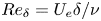 $Re_{\delta }=U_e \delta /\nu$ exceeds a critical value around 300 (Fransson et al. Reference Fransson, Brandt, Talamelli and Cossu2004). The instability is of viscous nature and the first amplified wave is the Tollmien–Schlichting wave (Schlichting & Gersten Reference Schlichting and Gersten2003). The unperturbed Blasius boundary layer can thus be linearly unstable for the considered Reynolds numbers in the present work. However, the presence of an isolated roughness element induces streaks, and for the streaks with sufficiently large magnitude, the inflection points can change the linear instability to an inviscid nature. The high- and low-speed streaks are examined in figure 8, using isosurfaces of the streamwise velocity deviation
  $u_d=\bar {u}-u_{bl}$. For case
  $(Re_h,\eta )=(600,1)$, the central low-speed streak and two lateral low-speed streaks are illustrated in figure 8(a). The central low-speed streak, which occurs symmetrically with respect to the mid-plane, originates from the flow separation downstream of the roughness element. The lateral low-speed streaks are associated with the counter-rotating vortices. High-speed streaks close to the wall appear farther downstream. Figure 8(b) shows that for case
  $(Re_h,\eta )=(600,0.5)$, the thinner roughness geometry leads to thinner and less sustainable central and lateral low-speed streaks, and the high-speed streaks are absent farther downstream. For case
  $(Re_h,\eta )=(800,0.5)$, figure 8(c) shows that the strength of the central and lateral low-speed streaks gets amplified as
  $Re_h$ increases. In contrast to the other two cases, the high-speed streaks are prominent in the near-wake regions, indicating increased spanwise shear that would contribute to the sinuous instability examined in § 4.2. Combining the above results and the smaller
  $h/\delta ^{*}$ results from Loiseau et al. (Reference Loiseau, Robinet, Cherubini and Leriche2014), it can be concluded that: first, larger
  $h/\delta ^{*}$, larger
  $\eta$ and higher
  $Re_h$ lead to a stronger wall-normal shear and a more sustainable central low-speed streak; second, increasing
  $Re_h$ for thin roughness could result in an increased spanwise shear in the near-wake region.
Top view (left) and 3-D view (right) of high- and low-speed streaks, visualized by isosurfaces of the streamwise velocity deviation of the base flow from the theoretical Blasius boundary layer solution,  $u_d=\bar {u}-u_{bl}$, for (a) case
  $(Re_h,\eta )=(600,1)$, (b) case
  $(Re_h,\eta )=(600,0.5)$, and (c) case
  $(Re_h,\eta )=(800,0.5)$.

4.2. Direct and adjoint analyses
4.2.1. Global stability analysis
Global stability analysis has been performed for cases with  $\eta =1$ and
  $\eta =0.5$ at different
  $Re_h$, and the leading eigenvalues are shown in figures 9(a) and 9(b), respectively. For
  $\eta =1$, one leading eigenvalue is obtained at each
  $Re_h$, as shown in figure 9(a). The case at
  $Re_h=450$ is stable, consistent with the steady flow field observed from the DNS results. As
  $Re_h$ increases, both the growth rate and the temporal frequency are increased. The critical
  $Re_h$ can be identified when the growth rate of an eigenvalue becomes positive. The flow at
  $Re_h=475$ is marginally stable, which suggests that the critical
  $Re_h$ is close to
  $475$ for this configuration.
Leading eigenvalues of cases with (a)  $\eta =1$ and (b)
  $\eta =0.5$, at different
  $Re_h$.

For  $\eta =1$, the eigenmodes of the leading eigenvalues are all varicose for the various
  $Re_h$ investigated. The real part of the leading eigenmodes is shown for
  $Re_h=475$ and
  $Re_h=600$ in figures 10(a) and 10(b). Both the leading stable and unstable global modes exhibit a varicose symmetry with respect to the spanwise mid-plane. As shown by the 3-D view of the eigenmode, the shape and location of the modes are consistent with those of the central low-speed streak observed in figure 8(a). The varicose mode demonstrates the unstable nature of the central low-speed region induced by the roughness element. Compared to the stable mode at
  $Re_h=475$, the unstable mode at
  $Re_h=600$ is more notably lifted, corresponding to the more raised shear layer for higher
  $Re_h$ observed in figure 7.
Contour plots at slice  $y=0.5h$ (left) and isosurfaces (right) of the streamwise velocity component of the leading unstable global modes, for (a) case
  $(Re_h,\eta )=(475,1)$, (b) case
  $(Re_h,\eta )=(600,1)$, and (c,d) case
  $(Re_h,\eta )=(800,0.5)$. The contour levels depict
  ${\pm }10\,\%$ of the mode's maximum streamwise velocity.

For  $\eta =0.5$, a different unstable behaviour is shown in figure 9(b). One leading stable eigenvalue is seen at
  $Re_h=450$, and its associated mode is varicose. Two leading eigenvalues are obtained at higher
  $Re_h$. The eigenvalue with larger growth rate and lower frequency is a varicose mode, and the other eigenvalue with smaller growth rate and higher frequency is a sinuous mode. For the thinner roughness geometry, the sinuous instability becomes more prominent as
  $Re_h$ increases. The associated varicose and sinuous eigenmodes of the leading eigenvalues for case
  $(Re_h,\eta )=(800,0.5)$ are visualized in figures 10(c) and 10(d). While the varicose mode is associated with the central low-speed streak observed in figure 8(c), the sinuous mode shows a larger streamwise extent along the central region. These results indicate that both varicose and sinuous oscillations exist in the wake flow, and the effect of sinuous instability could be more persistent on the transition process. Thus it can be concluded that for thin roughness with large
  $h/\delta ^{*}$, while the varicose instability is dominant, the sinuous instability can also be present. The onset of sinuous instability results from the interplay of small
  $\eta$ and increased
  $Re_h$, corresponding to the enhanced spanwise shear observed in the near wake of the base flow with increasing
  $Re_h$.
4.2.2. Production of disturbance kinetic energy
The production of disturbance kinetic energy provides insight into how and where the global modes extract their energy from the base flow. As illustrated by De Tullio et al. (Reference De Tullio, Paredes, Sandham and Theofilis2013) and Loiseau et al. (Reference Loiseau, Robinet, Cherubini and Leriche2014), the main contributions to the production of disturbance kinetic energy are the two terms
 \begin{equation} P_y={-}|\hat{u}|\,|\hat{v}|\,\frac{\partial{U_b}}{\partial y},\quad P_z={-}|\hat{u}|\,|\hat{w}|\,\frac{\partial{U_b}}{\partial z}. \end{equation}
The streamwise variation and spatial distribution of these two dominant terms are examined for cases  $(Re_h,\eta )=(600,1)$ and
  $(Re_h,\eta )=(800,0.5)$.
The spatial variations of  $P_y$ and
  $P_z$ in crossflow planes are depicted in figure 11. In combination with the production terms, the local shear is visualized by the solid contour lines of
  $u_s=((\partial \bar {u}/\partial y)^{2}+(\partial \bar {u}/\partial z)^{2})^{1/2}$ in figure 11, where
  $\bar {u}$ is the streamwise velocity of the base flow. For case
  $(Re_h,\eta )=(600,1)$, two planes at
  $x=5h$ and
  $x=10h$ are shown in figures 11(a) and 11(b). The contour lines of
  $u_s$ demonstrate the central low-speed streak and the lateral low-speed streaks on either side of the cube. With increasing downstream distance, both the central and lateral low-speed streaks rise, reach their maximum strength at about
  $x=10h$, and then fade away. The planes beyond
  $x=10h$ are not shown for the sake of brevity. The distributions of
  $P_y$ and
  $P_z$ show a coincidence with the locations of the streaks, indicating that the varicose mode extracts the energy from the wall-normal and spanwise shear of the base flow. These results confirm that the varicose mode demonstrates the instability of the entire 3-D shear layer (De Tullio et al. Reference De Tullio, Paredes, Sandham and Theofilis2013; Loiseau et al. Reference Loiseau, Robinet, Cherubini and Leriche2014).
Contours of  $P_y$ on the left and
  $P_z$ on the right in crossflow planes at: (a)
  $x=5h$ and (b)
  $x=10h$ for case
  $(Re_h,\eta )=(600,1)$; (c)
  $x=2.5h$ for the leading varicose mode of case
  $(Re_h,\eta )=(800,0.5)$; and (d)
  $x=2.5h$ for the leading sinuous mode of case
  $(Re_h,\eta )=(800,0.5)$. The contour levels are shown within the range from
  $-10^{-7}$ (blue) to
  $10^{-7}$ (red). The localized shear is depicted by the solid lines of
  $u_s=((\partial \bar {u}/\partial y)^{2}+(\partial \bar {u}/\partial z)^{2})^{1/2}$ from
  $0$ to
  $2$. The orange dashed lines show the location of the element.

The lateral low-speed streaks also make a contribution to the dominant production terms when  $h/\delta ^{*}$ is large. The mode extracts energy from the lateral streaks, as shown at
  $x=10h$ in figure 11(b). The top views of
  $P_y$ and
  $P_z$ for case
  $(Re_h,\eta )=(600,1)$ demonstrated in figure 12(a) display the contributions of the two lateral streaks more clearly. The large shear ratio
  $h/\delta ^{*}$ leads to stronger central and lateral streaks in the present case. Although the varicose mode extracts most of energy from the central low-speed streak, the contribution of the lateral streaks cannot be neglected for cases with large shear ratios.
Contours of  $P_y$ on the left and
  $P_z$ on the right in
  $x$–
$x$– $z$ planes at
  $y=0.75h$, for (a) the leading varicose mode of case
  $(Re_h,\eta )=(600,1)$, (b) the leading varicose mode, and (c) the leading sinuous mode of case
  $(Re_h,\eta )=(800,0.5)$. The contour levels are the same as in figure 11.

In contrast, the contours of  $P_y$ and
  $P_z$ for the leading varicose and sinuous modes of case
  $(Re_h,\eta )=(800,0.5)$ are shown in figures 11(c) and 11(d), respectively. The distribution of
  $P_y$ demonstrates that while the varicose mode extracts the energy from the top edge of the central streak, the sinuous mode extracts its energy from the lateral parts of the central streak. These results are consistent with the observation by Loiseau et al. (Reference Loiseau, Robinet, Cherubini and Leriche2014) for small
  $h/\delta ^{*}$ cylindrical roughness. For the thinner geometry (
 $\eta =0.5$), there is less fluid passing above the roughness element, and a stronger spanwise shear is seen, corresponding to the longer wall-normal extent for the lateral parts of the central streak, shown in figure 11(d). This suggests that the sinuous instability occurs due to the fact that it could extract more energy from the spanwise shear. The contour plots of
  $P_y$ and
  $P_z$ at
  $y=0.75h$ are shown in figures 12(b) and 12(c). The
  $P_y$ and
  $P_z$ distributions of the sinuous mode show a longer streamwise extent than those of the varicose mode, implying that the influence of sinuous instability on the wake flow could last farther downstream. Both the varicose and sinuous modes are able to extract some energy from the lateral streaks. The contribution of the lateral streaks is associated with the strength of the lateral streaks, which is more likely dependent on the shear ratio.
4.2.3. Adjoint sensitivity analysis
Understanding the dominant flow instability mechanisms and their sensitivity to velocity perturbations is key to devising strategies for trip-induced boundary layer transition. The adjoint perturbation velocity field highlights the regions most receptive to momentum forcing, which provides important information on how to trip the wake flow in the subcritical regime. The leading adjoint eigenvalues in table 3 show good agreement with their associated direct eigenmode counterpart for cases  $(Re_h,\eta )=(600,1)$ and
  $(Re_h,\eta )=(800,0.5)$. The streamwise velocity component of the leading adjoint modes in figure 13 shows that the sensitivity regions are located immediately upstream of the roughness element, as well as on the top edge of the separation region directly above and downstream of the roughness element. The sensitivity region is smaller for the thinner geometry. The adjoint mode is symmetric with respect to the spanwise mid-plane, corresponding to the direct varicose mode, and is anti-symmetric corresponding to the direct sinuous mode.
Isosurfaces of the leading adjoint modes (left) and the wavemaker (right), for (a) the leading varicose mode in case  $(Re_h,\eta )=(600,1)$, and the leading (b) varicose and (c) sinuous modes in case
 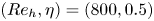 $(Re_h,\eta )=(800,0.5)$. The contour plots of the wavemaker are displayed with value 0.03.

Comparison of the leading eigenvalues of direct and adjoint modes for cases  $(Re_h,\eta )=(600,1)$ and
  $(Re_h,\eta )=(800,0.5)$.

Due to the large differences between the spatial distribution of direct and adjoint modes, neither direct nor adjoint solution alone can describe the whole picture. The product for each  $j$th pair of direct and adjoint global modes computed as
 \begin{equation} W_j(x,y,z) =\frac{\|\hat{u}^{j}\|\,\|\hat{u}^{{{\dagger}},j}\|}{\max(\|\hat{u}^{j}\|\,\|\hat{u}^{{{\dagger}},j}\|)} \end{equation}
determines the region where the eigenvalues of the LNS operator are most sensitive to localized feedback (Giannetti & Luchini Reference Giannetti and Luchini2007) – also called the ‘wavemaker’ regions. Locations where  $W \approx 1$ are sensitive to localized feedback, corresponding to the instability core. The value of
  $W$ can be interpreted as quantification of a possible change in the eigenvalues as a result of applied forcing in the given region of the flow (Ilak et al. Reference Ilak, Schlatter, Bagheri and Henningson2012).
The wavemaker results in figure 13 bring new insights in terms of the effects of different aspect ratios on the transition features. They show that the two geometries investigated in the present work result in different sensitivity natures of the shear layer. The maximum value of the wavemaker at each  $z$–
$z$– $y$ plane is plotted in figure 14 to demonstrate the strength variation of the wavemaker along the streamwise direction. For both
  $\eta =1$ and
  $\eta =0.5$, the wavemaker is strongest at the reversed flow region, indicating that the source of instability corresponds to the ‘roll-up’ of the shear layer. It then drops to the order of
  $10^{-1}$ as it passes through the reversed flow region. The sinuous mode in case
  $(Re_h,\eta )=(800,0.5)$ (figure 13c) shows that the region sensitive to localized feedback is dominated by the lateral sides of the shear layer, in contrast to the varicose mode showing only one primary sensitivity region.
Streamwise variation of the maximum of the wavemaker for the leading varicose mode in case  $(Re_h,\eta )=(600,1)$, and the leading varicose and sinuous modes in case
  $(Re_h,\eta )=(800,0.5)$. The vertical dashed lines denote the locations of cuboid origin and edges of the reversed flow regions.

The noteworthy difference between the two geometries is that a spatial transient growth of the wavemaker is seen for  $\eta =1$, but not seen for
  $\eta =0.5$. This indicates that for
  $\eta =1$, the roll-up motions are convected by the flow and could aid in the generation of hairpin vortices in the nonlinear evolution farther downstream, and the entire shear layer is sensitive to localized feedback. In contrast, for
  $\eta =0.5$, the spatial convective growth of the wavemaker is weak. A larger roughness aspect ratio induces a stronger central streak that is associated with a stronger spatial transient growth. The convective nature of the shear layer is thus more likely to depend on the strength of the central streak, rather than the types of instability.
4.3. Vorticity behaviour under different instabilities
To understand the influence of different instability characteristics on the behaviour of vortical structures in the wake flows, DNS combined with DMD analysis are performed for cases with  $\eta =1$ and
  $\eta =0.5$. Cases
  $(Re_h,\eta )=(600,1)$ and
  $(Re_h,\eta )=(800,0.5)$ are examined to better understand how vortical structures develop following different types of global instability.
4.3.1. Hairpin vortices
Figure 15 shows the vortical structures using isocontours of  $Q=0.05U_e^{2}/h^{2}$ (Chong, Perry & Cantwell Reference Chong, Perry and Cantwell1990). For case
  $(Re_h,\eta )=(600,1)$ in figure 15(a), the vortical motions induced by side edges of the cube interact with the shear layer generated over the cube, giving birth to the hairpin vortices. Both the primary hairpin vortices and secondary wall-attached vortices are observed downstream of the roughness element. These vortical structures are amplified and fragment into small structures beyond
  $x=18h$, which is a manifestation of transition. The vortex ‘head’ and ‘legs’ are advected, stretched downstream, and diminish after
  $x=44h$. It can be seen that the convective nature of the shear layer indicated by the wavemaker results assists the advection and amplification of the hairpin vortices farther downstream.
Visualizations of instantaneous vortical structures for (a) case  $(Re_h,\eta )=(600,1)$ by isocontours of
  $Q=0.1U_e^{2}/h^{2}$, and (b) case
  $(Re_h,\eta )=(800,0.5)$ by isocontours of
  $Q=0.05U_e^{2}/h^{2}$, coloured with streamwise velocity.

In contrast, case  $(Re_h,\eta )=(800,0.5)$ in figure 15(b) shows different vortical motions in the wake flow. As the horseshoe vortices wrap around the roughness element and interact with the shear layer, anti-symmetric distribution of vortical structures is seen in the immediate vicinity downstream of the roughness. This indicates that sinuous oscillations occur just downstream of the roughness element. The primary hairpin vortices modulated by the sinuous oscillations of the central streak also exhibit a sinuous wiggling. Since the spatial growth of the roll-up motions is weak as indicated by the wavemaker results, the hairpin vortices break down and fade away beyond
  $x=18h$, while the sinuous wiggling of the streaks continues farther downstream. It is thus clear that for case
  $(Re_h,\eta )=(800,0.5)$, varicose and sinuous instabilities have different influences on the behaviour and development of vortical structures. The effect of varicose instability is limited within a short streamwise extent and is unable to sustain the formation of hairpin vortices farther downstream. The sinuous instability that originates from the immediate roughness vicinity is correlated with the wiggling of the central streak and has a more persistent effect than the varicose instability on the wake flow.
The time history of streamwise velocity probed at three stations is examined for case  $(Re_h,\eta )=(600,1)$ in figure 16(a). Periodic oscillations with circular frequency
  $\omega =1.088$ are seen at different streamwise stations, corresponding to the periodic shedding of hairpin vortices. These self-sustained oscillations independent of external noise are a sign of global instability (Puckert & Rist Reference Puckert and Rist2018), and their frequency is close to the temporal frequency of the leading global varicose mode. For case
  $(Re_h,\eta )=(800,0.5)$, figure 16(b) shows that stronger fluctuations with multiple frequencies resulting from different instability characteristics are observed in the immediate vicinity of the roughness element, and smaller amplitude of velocity variations are seen at the farther downstream stations.
Time history of streamwise velocity variations for (a) case  $(Re_h,\eta )=(600,1)$, and (b) case
  $(Re_h,\eta )=(800,0.5)$, at three stations:
  $(x,y,z)=(5h,0.75h,0)$ (solid),
  $(x,y,z)=(12h,0.75h,0)$ (dashed) and
  $(x,y,z)=(20h,0.75h,0)$ (long dashed).

4.3.2. Energy and DMD spectra analyses
To understand the dynamics behind this different behaviour for cases  $(Re_h,\eta )=(600,1)$ and
  $(Re_h,\eta )=(800,0.5)$, DMD was performed and compared to the energy spectra and global stability results. DMD is a data-driven modal decomposition technique that identifies a set of modes from multiple snapshots of the observable vectors. Each of the DMD modes has an assigned eigenvalue that describes its temporal growth/decay rate and oscillation frequency. DMD is a useful tool to isolate the regions associated with a particular frequency and provide information on system dynamics. For the present work, we use a novel DMD algorithm developed by Anantharamu & Mahesh (Reference Anantharamu and Mahesh2019) that is suitable for analysis of large datasets. The basic idea behind DMD is that the set of snapshot vectors of flow variables
  $\{ \psi _i \}_{i=1}^{N-1}$ can be written as a linear combination of DMD modes
  $\{ \phi _i \}_{i=1}^{N-1}$ as
 \begin{equation} \psi_i = \sum_{j=1}^{N-1} c_j \lambda_j \phi_j,\quad i=1,\ldots, N-1, \end{equation}
where  $\lambda _j$ are the eigenvalues of the projected linear mapping and
  $c_j$ are the
  $j$th entries of the first vector
  $\psi _1$. The detailed derivation of the algorithm can be obtained from Anantharamu & Mahesh (Reference Anantharamu and Mahesh2019). To ensure the accuracy of the results,
  $N=200$ snapshots of the flow field were taken with
  $\Delta t\,U_e/h=0.15$ between them for case
  $(Re_h,\eta )=(600,1)$, and
  $N=700$ snapshots were taken with
  $\Delta t\,U_e/h=0.1$ between them for case
  $(Re_h,\eta )=(800,0.5)$.
Also, power spectral density (PSD) is examined at the mid-plane for different streamwise stations downstream of the roughness. For case  $(Re_h,\eta )=(600,1)$, the PSD shows a primary peak at the Strouhal number
  $St=0.175$ in figure 17(a), corresponding to the shedding frequency of the main hairpin vortices and the secondary wall-attached vortices observed in figure 15(a). The interaction between different vortical structures results in the higher harmonics at
  $St=0.35$ and
  $0.525$. Note that similar peaks are also identified in the DMD spectra (figure 17c). Table 4 demonstrates a comparison of the eigenvalues and Strouhal numbers obtained from global stability and DMD analyses. The Strouhal numbers obtained from global stability analysis and DMD analysis show good agreement. The associated global unstable mode of the mean flow and the DMD mode are examined in figure 18. They both demonstrate varicose features and show good qualitative agreement.
Comparison between the energy spectra of streamwise velocity at different  $x$ stations for (a) case
  $(Re_h,\eta )=(600,1)$ and (b) case
  $(Re_h,\eta )=(800,0.5)$, and the DMD spectra of the last snapshot for (c) case
  $(Re_h,\eta )=(600,1)$ and (d) case
  $(Re_h,\eta )=(800,0.5)$. The power spectral density (PSD) has been non-dimensionalized as
  $PSD=E/(U_e h)$.

Comparison between (a) the leading global unstable mode of the mean flow and (b) the DMD mode at  $St=0.175$ for case
  $(Re_h,\eta )=(600,1)$, depicted by isocontours of the streamwise velocity component. The contour levels depict
  ${\pm }10\,\%$ of the mode's maximum streamwise velocity.

Comparison of the eigenvalues from global stability and DMD analyses for case  $(Re_h,\eta )=(600,1)$.

Compared to case  $(Re_h,\eta )=(600,1)$, a combination of multiple frequencies is distributed in the energy and DMD spectra for case
  $(Re_h,\eta )=(800,0.5)$, indicating more complicated flow behaviour. Figure 17(b) shows that the peaks at
  $St=0.210$ and
  $St=0.321$ are close to the temporal frequency of the varicose and sinuous modes obtained from global stability analysis. Similar peaks are also seen in the DMD spectra from figure 17(d). The associated DMD modes are examined in figures 19(b) and 19(c). The varicose and sinuous symmetries are seen for the DMD modes at
  $St=0.210$ and
  $0.321$, which is consistent with the global stability results. The higher harmonic peaks at
  $St=0.420$,
  $0.537$,
  $0.630$ and
  $0.840$ are evident in the vicinity downstream of the roughness element (
 $x=5h$), resulting from the interactions between the varicose and sinuous oscillations in the near-wake region. The DMD spectra show agreement with the energy spectra for the higher harmonics. The associated DMD modes at
  $St=0.416$ and
  $St=0.623$ are varicose since they are the higher multiples of the varicose mode at
  $St=0.208$, while the DMD mode at
  $St=0.520$ is sinuous due to a superposition of the varicose mode at
  $St=0.208$ and the sinuous mode at
  $St=0.312$. The results indicate that the interactions between the hairpin vortices and the general sinuous oscillations are significant in the near wake, and diminish as the vortical structures develop farther downstream. With increasing streamwise distance, a peak at a low frequency
  $St=0.120$ in figure 17(b) gets amplified. This peak is also captured in the DMD spectra (figure 17d). The corresponding DMD mode in figure 19(a) shows a sinuous symmetry. This sinuous mode is associated with the wiggling of the streaks observed farther downstream in figure 15(b). It is thus clear that for a thin geometry with a large
  $h/\delta ^{*}$, the sinuous mode that occurs at higher
  $Re_h$ can interact with the hairpin vortices, and lead to different wake flow behavior in the transition process.
The DMD modes for case  $(Re_h,\eta )=(800,0.5)$ at (a)
  $St=0.115$, (b)
  $St=0.208$, (c)
  $St=0.312$, (d)
  $St=0.416$, (e)
  $St=0.520$ and ( f)
  $St=0.623$, depicted by isocontours of the streamwise velocity component. The contour levels depict
  ${\pm }10\,\%$ of the mode's maximum streamwise velocity.

4.4. Nonlinear breakdown to turbulence
Getting a canonical turbulent boundary layer as early as possible is the primary goal to design an effective trip. The joint effects of the two geometries and an increasing  $Re_h$ on the nonlinear evolution to turbulence are investigated. Longer streamwise domain lengths are used to examine the transition to turbulence.
4.4.1. Transition and instability diagrams
The roughness Reynolds number is one of the important parameters in roughness-induced transition. The definition of  $Re_h$ does not account for the impact of the relative location of the roughness element in a boundary layer. Another definition,
  $Re_{hh}=u_{h}h/\nu$, based on the Blasius velocity solution at the roughness tip location
  $u_h$, has been suggested to best characterize roughness-induced transition (Klanfer & Owen Reference Klanfer and Owen1953). Von Doenhoff & Braslow (Reference Von Doenhoff and Braslow1961) have suggested a transition diagram that correlates the roughness aspect ratio
  $\eta$ with
  $Re_{hh}$, and can be used to predict the transition features.
Dependence of the transition process on  $\eta$ and
  $Re_{hh}$ is examined for the present cases by reproducing the transition diagram in figure 20(a). Cases located in region (i) (below the lower curve) are expected to have a steady wake flow, cases fitting into region (ii) (between the lower and upper curves) indicate that the wake flow is unsteady and transition occurs, and for cases situated in region (iii) (above the upper curve), transition occurs immediately downstream of the roughness. The correlation between
  $\eta$ and
  $Re_{hh}$ revealed by figure 20(a) shows that for roughness elements with
  $0.6 \leqslant \eta \leqslant 2$,
  $\eta$ plays a more important role in the onset of unsteadiness than the onset of immediate transition downstream of roughness, while the opposite effect is seen for roughness with
  $0.3 \leqslant \eta \leqslant 0.6$.
(a) Reproduced von Doenhoff–Braslow transition diagram; (b) scaling the data to cluster different types of instability. Diamonds represent the present work; rectangles denote data from Loiseau et al. (Reference Loiseau, Robinet, Cherubini and Leriche2014); circles denote data from Citro et al. (Reference Citro, Giannetti, Luchini and Auteri2015); triangles denote data from Bucci et al. (Reference Bucci, Cherubini, Loiseau and Robinet2021). The symbols in purple denote sinuous modes, in blue denote varicose modes, in green represent the case that transition occurs immediately downstream and global instability has not been applied.

Corresponding to the transition diagram, the associated flow behaviour in the transition process is examined in figure 21. For  $\eta =1$, the stable cases at
  $Re_h=450$ are located in region (i), consistent with a stable wake flow in global stability and DNS results. The unstable cases at
  $Re_h=600$ and
  $800$ are within region (ii), and the transition process is examined in figures 21(a) and 21(b), respectively. For case
  $(Re_h,\eta )=(600,1)$, both the near and farther wakes are symmetric with respect to the spanwise mid-plane, corresponding to the leading unstable varicose mode. For case
  $(Re_h,\eta )=(800,1)$, symmetric fluid motions with smaller length scales are seen in the near-wake region, indicating that nonlinear breakdown occurs more closely downstream of the roughness as
  $Re_h$ increases. Intense shear between streaks results in spanwise oscillations in the farther wake. Although only the varicose global instability is detected for this configuration, a sinuous-like breakdown could happen when
  $Re_h$ is sufficiently high. This sinuous breakdown might be related or subsequently lead to secondary sinuous instabilities observed by Denissen & White (Reference Denissen and White2013) and Vadlamani, Tucker & Durbin (Reference Vadlamani, Tucker and Durbin2018), which would destabilize the shear layer and promote transition to turbulence. Note that whether or not the unstable cases undergo transition to turbulence is not revealed in this transition diagram since the effects on other configuration parameters, such as spanwise spacing and
  $Re_{\delta }$, need to be considered. Case
  $(Re_h,\eta )=(1100,1)$ is located in region (iii), suggesting that immediate transition downstream of the roughness is expected, which is verified in figure 21(c). The streamwise streaks identified farther downstream imply that transition to fully-developed turbulence might occur.
Contour plots of instantaneous streamwise velocity field at slice  $y=0.5h$, for cases with
  $\eta =1$ at (a)
  $Re_h=600$, (b)
  $Re_h=800$ and (c)
  $Re_h=1100$, and cases with
  $\eta =0.5$ at (d)
  $Re_h=600$, (e)
  $Re_h=800$ and ( f)
  $Re_h=1100$.

The  $\eta =0.5$ cases are also demarcated by the transition diagram. The unstable case at
  $Re_h=600$ is slightly off from region (ii) since roughness with sharp edges results in a lower
  $Re_{hh}$ for unsteadiness to occur than other smoother roughness geometries. Figure 21(d) shows that the wake flow at
  $Re_h=600$ displays a thinner symmetric central streak compared to that of
  $\eta =1$. There are no sinuous oscillations observed since the sinuous mode is marginally stable at
  $Re_h=600$. As
  $Re_h$ increases to
  $800$ (figure 21e), the anti-symmetric oscillations in the spanwise direction become evident in both the near and farther wakes, associated with the more prominent sinuous instability, and a persistent effect of sinuous oscillations is seen farther downstream. For
  $Re_h=1100$ (figure 21f), the sinuous oscillations can still be observed in the near-wake region. The wake flow is thinner compared to that of
  $\eta =1$, indicating that the interactions between the wake flows at spanwise boundaries might occur farther downstream.
Combined with the present cases, the data from previous work are also shown in figure 20(a), and the instability types are denoted by different colours. Although the transition diagram in figure 20(a) can predict the transition onsets, it fails to classify the associated different instability mechanisms due to the joint effects of  $\eta$ and
  $h/\delta ^{*}$. We therefore develop a new correlation between
  $Re_{hh}^{1/2}$ and
  $d/\delta ^{*}$ in figure 20(b). By using
  $d/\delta ^{*}$ to rescale the data, the cases with either varicose or sinuous instability are clustered separately. The decision boundary denoted by
  $Re_{hh}^{1/2}=2.81d/\delta ^{*}+21.49$ in figure 20(b) is obtained by logistic regression model (Hosmer, Lemeshow & Cook Reference Hosmer, Lemeshow and Sturdivant2000) to demarcate the two instability types. The parameters in the decision boundary are determined using an unconstrained optimization algorithm (Gill & Murray Reference Gill and Murray1972). This diagram suggests that the sinuous instability occurs when
  $d/\delta ^{*}$ is relatively small and
  $Re_{hh}^{1/2}$ is higher than a certain threshold. It is therefore useful to predict the instability mechanisms in the wake flow based on a different combination of configuration parameters, with no need of visual inspection of the flow fields.
4.4.2. Mean flow characteristics
The evolution to a turbulent state for the two geometries at  $Re_h=1100$ is examined by mean skin friction coefficient in figure 22. In the immediate vicinity of roughness location, the mean skin friction is smaller for
  $\eta =1$, due to the larger and stronger flow separation induced both upstream and downstream of the cuboids. In the range from
  $x=8h$ to
  $x=90h$, the
  $C_f$ value increases gradually due to the nonlinear breakdown, and the
  $C_f$ of
  $\eta =0.5$ presents a value lower than that of
  $\eta =1$. This results from the thinner wake flow associated with the thinner roughness geometry. The
  $C_f$ value peaks at
  $x \approx 80h$ for
  $\eta =1$, and at
  $x \approx 90h$ for
  $\eta =0.5$. The two
  $C_f$ curves then decay farther downstream and collapse with each other, as a manifestation of establishing turbulent boundary layers.
Streamwise variation of time-averaged and spanwise-averaged skin friction for  $\eta =1$ and
  $\eta =0.5$ at
  $Re_h=1100$. The roughness location is denoted by the grey area.

The boundary layer evolution from laminar to turbulent states is shown in figure 23(a) using the mean velocity profiles in wall units at different streamwise locations downstream of the roughness element. The roughness geometry with  $\eta =1$ presents an earlier location of an establishment of a fully turbulent state. We show the results of only case
  $(Re_h,\eta )=(1100,1)$ for the sake of brevity. The time-averaged streamwise velocity at the mid-plane is normalized by the local friction velocity
  $u_{\tau }$, where
  $u_{\tau }$ is computed from the
  $C_f$ profile at
  $z=0$ for each
  $x$ location. The wall-normal coordinate in wall units is
  $y^{+}=yu_{\tau }/\nu$. The results show that all profiles collapse well in the viscous sublayer and follow the correlation
  $U^{+}=y^{+}$. From
  $x=5h$ to
  $x=40h$, significant increase is observed above the viscous layer, which is due to the lift-up behaviour of the shear layer. The mean velocity profile above the viscous sublayer reaches its maximum magnitude at
  $x=40h$ and decreases to approach the log-law profile as the
  $x$ location increases farther downstream. Agreement with the logarithmic law is seen beyond
  $x=100h$, indicating that the inner layer is fully developed. As the
  $x$ location increases even farther, the profiles at
  $x=110h$ and
  $x=130h$ show agreement in both the inner and outer layers, suggesting that fully developed turbulent flow is established in both the inner and outer layers. The velocity fluctuations and Reynolds shear stresses at
  $x=130h$ are depicted in figure 23(b) using wall scaling. The velocity fluctuations
  $u_{rms}$,
  $v_{rms}$ and
  $w_{rms}$ are normalized by
  $u_{\tau,ave}$, and the Reynolds shear stress
  $\langle u'v' \rangle$ is normalized by
  $u_{\tau,ave}^{2}$, where
  $u_{\tau,ave}$ is the spanwise-averaged friction velocity computed from the spanwise-averaged
  $C_f$ at
  $x=130h$. The results show good agreement with the results of a turbulent zero-pressure-gradient boundary layer from Schlatter et al. (Reference Schlatter, Li, Brethouwer, Johansson and Henningson2010).
(a) Mean velocity profiles in wall units at different streamwise stations for case  $(Re_h,\eta )=(1100,1)$. (b) Reynolds stresses for case
  $(Re_h,\eta )=(1100,1)$ at
  $x=130h$ (corresponding to
  $Re_{\tau }=272$) compared with the large-eddy simulations of Schlatter et al. (Reference Schlatter, Li, Brethouwer, Johansson and Henningson2010) at
  $Re_{\tau }=257$.

5. Conclusions
Global stability analysis and direct numerical simulation are performed to study roughness-induced transition. Isolated cuboids with small aspect ratios  $\eta =1$ and
  $0.5$ are investigated at different
  $Re_h$. The ratio
  $h/\delta ^{*}=2.86$ is larger than in most past studies, representative of the effects of a large protuberance on the transition process.
Understanding the differences between the base and mean flows is crucial to choosing an appropriate base state for linear stability analysis. Our results show that using either the base flow or the mean flow as the base state for global stability analysis is able to capture the shedding frequency of the primary vortical structures and the associated mode shapes. However, the mean flow evolves to a marginally stable state due to the nonlinear saturation, in contrast to an unstable base flow. This suggests that for roughness-induced transition, using base flows can better predict the instability onset, while using mean flows is also meaningful and can serve as an alternative base state for linear stability analyses.
The streak properties play an important role in instability characteristics, and their dependence on the configuration parameters is investigated. Combined with past studies with small  $h/\delta ^{*}$ (Loiseau et al. Reference Loiseau, Robinet, Cherubini and Leriche2014), it can be summarized that higher
  $Re_h$, larger
  $\eta$ and higher
  $h/\delta ^{*}$ lead to a stronger wall-normal shear and a more sustainable central streak. Also, as
  $Re_h$ increases for the thinner geometry (
 $\eta =0.5$), high-speed streaks below the central streak become prominent in the near-wake region, indicating an increased spanwise shear that can contribute to sinuous instability.
Global stability analysis shows that when the shear ratio is sufficiently high ( $h/\delta ^{*}=2.86$), the varicose instability is dominant for the roughness element with small aspect ratios (
 $\eta \leqslant 1$). For
  $\eta =1$, both the stable and unstable modes exhibit varicose symmetry. For
  $\eta =0.5$, the varicose instability is dominant at different
  $Re_h$, and the sinuous instability becomes more pronounced as
  $Re_h$ increases. These results complement what has been reported in Loiseau et al. (Reference Loiseau, Robinet, Cherubini and Leriche2014) and Bucci et al. (Reference Bucci, Puckert, Andriano, Loiseau, Cherubini, Robinet and Rist2018) by showing that the sinuous instability can also be observed when
  $\eta$ is sufficiently small for a large
  $h/\delta ^{*}$. The production of disturbance kinetic energy highlights that the sinuous mode extracts its energy from the lateral parts of the central streak, and thus becomes more prominent with an increased spanwise shear in the near wake. It is also shown that for large
  $h/\delta ^{*}$, the lateral streaks are strong and they also make a contribution to the energy extraction.
The wavemaker that considers both direct and adjoint modes provides important information on the receptivity and inception of global instability. The results show that the instability core is located in the reversed flow region for both varicose and sinuous modes. Loiseau et al. (Reference Loiseau, Robinet, Cherubini and Leriche2014) suggest that a large spatial transient growth is observed along the central streak for the varicose mode, and that is not seen for the sinuous mode. Our results, however, indicate that this convective nature of the shear layer is more prominent for a stronger central streak, and thus is more likely to depend on the roughness aspect ratio, rather than different instability types.
The associated vortical structures and transitional flow behaviour corresponding to different instability mechanisms are compared for the two geometries. For  $\eta =1$, the single and dominant peak corresponding to the hairpin vortex shedding and its higher harmonics show agreement in energy and DMD spectra, in accordance with the eigenfrequency of the leading varicose mode. The convective nature of the shear layer assists the formation of hairpin vortices farther downstream. In contrast to
  $\eta =1$, the sinuous wiggling of hairpin vortices becomes prominent in the near wake as
  $Re_h$ increases for
  $\eta =0.5$. The varicose and sinuous modes are not perfect harmonics, and their interactions result in a broad-banded response in the energy and DMD spectra. The hairpin vortices break down and fade away within a shorter distance, and a sinuous mode associated with the wiggling of streaks persists farther downstream. For both geometries with an increasing
  $Re_h$, transition occurs closer to the roughness element, and sinuous-like breakdown is seen farther downstream, destabilizing the shear layer and promoting transition to turbulence.
While the transition onsets are well predicted by the transition diagram from Von Doenhoff & Braslow (Reference Von Doenhoff and Braslow1961), it is unable to predict different instability characteristics in the transition process. We develop a new diagram demonstrating the correlation between  $Re_{hh}^{1/2}$ and
  $d/\delta ^{*}$. The cases that present either varicose or sinuous instability with various
  $h/\delta ^{*}$,
  $\eta$ and
  $Re_{hh}$ from the previous and present studies are clustered separately in this diagram. This diagram can thus be used to classify and predict the associated instability mechanisms in roughness wakes based on different combinations of configuration parameters, with no need of visual inspection of the flow field. Finally, the trip effects on the mean skin friction and the evolution to turbulence are compared for the two geometries. Although the
  $C_f$ value for
  $\eta =1$ is higher in general during the transition process, and peaks at an earlier location, it collapses with
  $C_f$ of
  $\eta =0.5$ beyond
  $x \approx 90h$, indicating that both geometries are efficient to trip the flow to turbulence. For
  $\eta =1$, a fully-developed turbulent state is established in both the inner and outer layers at
  $x \approx 110h$.
Funding
This work was supported by the United States Office of Naval Research (ONR) grant N00014-17-1-2308 and N00014-20-1-2717 managed by Dr P. Chang. Computing resources were provided by the Minnesota Supercomputing Institute (MSI) and Extreme Science and Engineering Discovery Environment (XSEDE).
Declaration of interests
The authors report no conflict of interest.


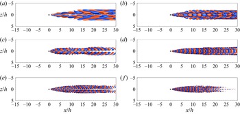


 Open access