The DESC stellarator code suite. Part 1. Quick and accurate equilibria computations

D. Panici; R. Conlin; D.W. Dudt; K. Unalmis; E. Kolemen

doi:10.1017/S0022377823000272

The DESC stellarator code suite. Part 1. Quick and accurate equilibria computations

Published online by Cambridge University Press: 18 May 2023

and

D. Panici: Affiliation:
Princeton University, Princeton, NJ 08544, USA
R. Conlin: Affiliation:
Princeton University, Princeton, NJ 08544, USA
D.W. Dudt: Affiliation:
Princeton University, Princeton, NJ 08544, USA
K. Unalmis: Affiliation:
Princeton University, Princeton, NJ 08544, USA
E. Kolemen*: Affiliation:
Princeton University, Princeton, NJ 08544, USA
*: †Email address for correspondence: ekolemen@princeton.edu

Article contents

Abstract
Introduction
Literature review
Code descriptions
Comparison methods
Results
Conclusions
Funding
Declaration of interests
Data availability statement
References

Rights & Permissions

Abstract

Three-dimensional equilibrium codes are vital for stellarator design and operation, and high-accuracy equilibria are also necessary for stability studies. This paper details comparisons of two three-dimensional equilibrium codes: VMEC, which uses a steepest-descent algorithm to reach a minimum-energy plasma state, and DESC, which minimizes the magnetohydrodynamic (MHD) force error in real space directly. Accuracy as measured by satisfaction of MHD force balance is presented for each code, along with the computation time. It is shown that DESC is able to achieve more accurate solutions, especially near axis. The importance of higher-accuracy equilibria is shown in DESC's better agreement of stability metrics with asymptotic formulae. DESC's global Fourier–Zernike basis also yields solutions with analytic derivatives explicitly everywhere in the plasma volume, provides improved accuracy in the radial direction versus conventional finite differences and allows for exponential convergence. Further, DESC can compute a solution with the same accuracy as VMEC in order-of-magnitude less time.

Keywords

plasma confinement fusion plasma plasma simulation

Type: Research Article
Information: Journal of Plasma Physics , Volume 89 , Issue 3 , June 2023 , 955890303

DOI: https://doi.org/10.1017/S0022377823000272 [Opens in a new window]

NASA ADS Abstract Service [Opens in a new window]
Creative Commons: This is an Open Access article, distributed under the terms of the Creative Commons Attribution licence (http://creativecommons.org/licenses/by/4.0/), which permits unrestricted re-use, distribution and reproduction, provided the original article is properly cited.
Copyright: Copyright © The Author(s), 2023. Published by Cambridge University Press

1. Introduction

In the design of any fusion device, the preliminary step is the computation of a plasma equilibrium state with the desired geometry. A plasma in an equilibrium state can be described by the ideal magnetohydrodynamic (MHD) equilibrium model:

(1.1a)\begin{gather} \boldsymbol{J}\times \boldsymbol{B} = \boldsymbol{\nabla} p, \end{gather}

(1.1b)\begin{gather} \boldsymbol{\nabla} \times \boldsymbol{B} = \mu_0 \boldsymbol{J}, \end{gather}

(1.1c)\begin{gather} \boldsymbol{\nabla} \boldsymbol{\cdot} \boldsymbol{B} = 0, \end{gather}

where $\boldsymbol {B}$ is the magnetic field, $\boldsymbol {J}$ is the current density, $p$ is the scalar pressure and $\mu _0$ is the permeability of free space. The satisfying of these equations implies that the plasma is in perfect force balance, i.e.

(1.2)\begin{equation} \boldsymbol{F} = \boldsymbol{J}\times \boldsymbol{B} - \boldsymbol{\nabla} p = 0 \end{equation}

everywhere in the plasma, and the plasma state also coincides with a stationary state in the plasma potential energy,

(1.3)\begin{equation} W = \int_V \left(\frac{B^2}{2\mu_0} + \frac{p}{\gamma -1} \,{\rm d}V \right), \end{equation}

where $V$ is the plasma volume and $\gamma$ is the adiabatic index.

In tokamaks, the plasma is typically taken to be axisymmetric, allowing the MHD equilibrium to be described by the Grad–Shafranov equation, for which there exist analytic solutions (Cerfon & Freidberg Reference Cerfon and Freidberg2010; Guazzotto & Freidberg Reference Guazzotto and Freidberg2021) and efficient codes to numerically solve for equilibria (Lao et al. Reference Lao, John, Stambaugh, Kellman and Pfeiffer1985). However, the problem becomes much more difficult without the assumption of axisymmetry, making stellarator equilibria more challenging to compute. Adding to the challenge are the singular currents predicted by ideal MHD to form at rational surfaces in three-dimensional (3-D) geometries (Helander Reference Helander2014). While this is an important topic to note, it is not elaborated upon in this work and is left to future endeavours.

Very few analytical solutions to the general 3-D equilibrium problem are known (Rosenbluth, Dagazian & Rutherford Reference Rosenbluth, Dagazian and Rutherford1973), and so typically 3-D equilibria must be found numerically. Thus, a fast, robust and accurate 3-D equilibrium solver is necessary for stellarator optimization studies. The current workhorse code for 3-D equilibria is VMEC (Variational Moments Equilibrium Code) (Hirshman & Whitson Reference Hirshman and Whitson1983), which is integrated into all current stellarator optimization workflows (Spong et al. Reference Spong, Hirshman, Whitson, Batchelor, Carreras, Lynch and Rome1998; Drevlak et al. Reference Drevlak, Beidler, Geiger, Helander and Turkin2019; Lazerson et al. Reference Lazerson, Schmitt, Zhu and Breslau2020; Landreman et al. Reference Landreman, Medasani, Wechsung, Giuliani, Jorge and Zhu2021). While a relatively robust and widely used code, VMEC still suffers from shortcomings stemming from its issues at the axis and its radial discretization, as well as its legacy design. A new 3-D stellarator equilibrium code, DESC (Dudt & Kolemen Reference Dudt and Kolemen2020; Dudt et al. Reference Dudt, Conlin, Panici, Unalmis, Kim and Kolemen2022), has been developed which can overcome these issues.

In this first part of a three-part series on DESC, a comparison of DESC and VMEC equilibria is conducted to show the advantages of DESC's equilibrium solver. Section 2 reviews the existing 3-D equilibrium codes, while section 3 details the two codes compared in this paper, VMEC and DESC. Section 4 defines the method of comparison and accuracy metrics used and section 5 presents the results of the comparison of accuracy in terms of equilibrium solution and stability calculations.

Part 2 (Conlin et al. Reference Conlin, Dudt, Panici and Kolemen2023) of the three-part series presents a novel perturbation and continuation method used by the DESC code for solving and optimizing stellarator equilibria. The efficiency and utility of the method are shown in the computation of complicated equilibria, highlighting the benefits of automatic differentiation. Part 3 (Dudt et al. Reference Dudt, Conlin, Panici and Kolemen2023) presents DESC's unique stellarator optimization capabilities made possible by the efficient equilibrium solver and the perturbation method described in the earlier parts, resulting in a speed-up in optimization by orders of magnitude. These advantages are shown in the context of quasi-symmetry optimization, where results are compared with conventional tools (Spong et al. Reference Spong, Hirshman, Whitson, Batchelor, Carreras, Lynch and Rome1998; Lazerson et al. Reference Lazerson, Schmitt, Zhu and Breslau2020). Three different quasi-symmetry objective formulations are also shown, with the relative advantages of each compared, highlighting the flexibility of DESC as an optimization code.

2. Literature review

Kruskal & Kulsrud (Reference Kruskal and Kulsrud1958) first formulated solutions to the ideal MHD equilibrium problem as a variational principle, and showed that solutions to (1.1) are toroidal equilibria with nested flux surfaces and with pressure as a flux function. The earliest 3-D equilibrium codes utilized this principle, and discretized the spatial coordinates using finite difference schemes (Betancourt & Garabedian Reference Betancourt and Garabedian1976). The BETA code used an inverse coordinate mapping and second-order finite differences motivated by the variational principle to minimize energy and calculate equilibria (Bauer, Betancourt & Garabedian Reference Bauer, Betancourt and Garabedian1978). Later, Chodura & Schlüter (Reference Chodura and Schlüter1981) found equilibria numerically by minimizing $W$ on an Eulerian cylindrical grid.

Eventually, spectral codes (using Fourier series representations in the poloidal and toroidal angles) were employed, which were shown to be substantially more efficient in calculating equilibria than pure difference methods. Schwenn (Reference Schwenn1984) created FIT as a spectral upgrade of the TUBE equilibrium code. Bhattacharjee, Wiley & Dewar (Reference Bhattacharjee, Wiley and Dewar1984) derived a variational method with a spectral Fourier series in angle and Hermite cubic B-splines in the radial direction, and used both a conventional inverse mapping and a mixed coordinate mapping. Hender's NEAR code (Hender et al. Reference Hender, Carreras, Garcia, Rome and Lynch1985) used the same methodology as that of Chodura & Schlüter (Reference Chodura and Schlüter1981), but replaced the cylindrical coordinate system with vacuum flux coordinates and Fourier-decomposed the problem in both angles. Hirshman & Whitson (Reference Hirshman and Whitson1983) detailed the VMEC code, which also solved the inverse equilibrium problem based on the variational principle and using poloidal and toroidal Fourier series. VMEC is widely used in the stellarator community for the improvement its formulation had over existing equilibrium codes, although the radial discretization can lead to inaccuracy near the axis, and is discussed more in section 3.1. Additionally, an updated version of VMEC, GVEC, is currently being developed (Bañón Navarro et al. Reference Bañón Navarro, Merlo, Plunk, Xanthopoulos, von Stechow, Di Siena, Maurer, Hindenlang, Wilms and Jenko2020; Hudson et al. Reference Hudson, Loizu, Zhu, Qu, Nührenberg, Lazerson, Smiet and Hole2020). DESC (Dudt & Kolemen Reference Dudt and Kolemen2020; Dudt et al. Reference Dudt, Conlin, Panici, Unalmis, Kim and Kolemen2022) is a recent pseudospectral code which employs a spectral Fourier–Zernike basis in all three coordinates, and finds equilibria by satisfying the MHD force balance (1.1a) directly at collocation nodes. This choice of spectral basis automatically satisfies the necessary constraints at the axis for analytic functions, and the code is explained more in section 3.2. Each of these codes assumes nested flux surfaces, so multiple magnetic axes (i.e. islands) cannot be represented in their equilibrium representation.

Other 3-D equilibrium codes have been created which are able to handle islands and even chaotic regions. PIES (Reiman & Greenside Reference Reiman and Greenside1986) solves for the equilibrium magnetic field by iteratively evolving pressure-driven currents and re-solving for $\boldsymbol {B}$ with Ampere's law, solving the differential equations by angular Fourier decomposition and finite differences for the radial discretization. The BETA code was rewritten as the spectral (in angles) BETAS code (Betancourt Reference Betancourt1988), which used a coordinate system capable of representing non-nested flux surfaces, and later was the basis of the NSTAB (Taylor Reference Taylor1994) 3-D equilibrium and stability code. NSTAB used a method of finding the magnetic axis location using a residue condition obtained from the variational principle, as opposed to constraining the axis location based on linear interpolation or Taylor expansion as done by previous codes. SIESTA (Hirshman, Sanchez & Cook Reference Hirshman, Sanchez and Cook2011) is an iterative equilibrium solver, similar to PIES but based on the energy principle, which can handle more complicated magnetic field topologies than BETAS, and relies on a VMEC solution for initialization of the solving procedure. The HINT2 code (Suzuki et al. Reference Suzuki, Nakajima, Watanabe, Nakamura and Hayashi2006) solves the MHD equilibrium problem by introducing artificial viscosity and resistivity to the resistive MHD equations and relaxing to an equilibrium state on an Eulerian grid, without any assumption of nested flux surfaces. SPEC (Hudson et al. Reference Hudson, Dewar, Dennis, Hole, McGann, von Nessi and Lazerson2012) also uses a relaxation method, but in the MRxMHD framework, solving for equilibria using stepped, discontinuous pressure profiles. This method allows for very complicated magnetic field topology, but at the expense of requiring input profiles that may not be realistic. SPEC has recently implemented Zernike polynomials as their radial basis at the magnetic axis, which effectively handles the coordinate singularity present there, similar to DESC (Hudson et al. Reference Hudson, Loizu, Zhu, Qu, Nührenberg, Lazerson, Smiet and Hole2020; Qu et al. Reference Qu, Pfefferlé, Hudson, Baillod, Kumar, Dewar and Hole2020).

3. Code descriptions

3.1. VMEC

The most widely used 3-D equilibrium code in the stellarator community at present is VMEC (Hirshman & Whitson Reference Hirshman and Whitson1983). VMEC constructs equilibria by minimizing the MHD energy (1.3) through a variational principle. The base geometry is a cylindrical coordinate system $\boldsymbol {x} = (R,\phi,Z)$. VMEC uses as its computational grid the coordinates $\boldsymbol {\alpha } = (s,u,v)$, with $s$ being a radial coordinate proportional to the normalized toroidal flux, $u$ a poloidal-like angle and $v$ is the geometric toroidal angle (i.e. same as cylindrical $\phi$):

(3.1a)\begin{gather} s = \frac{\psi}{\psi}_a, \quad 0\leq s \leq 1, \end{gather}

(3.1b)\begin{gather} u = \theta^* - \lambda(s,u,v), \quad 0\leq u \leq 2{\rm \pi}, \end{gather}

(3.1c)\begin{gather} v = \phi, \quad 0\leq v \leq 2{\rm \pi}/N_{FP}, \end{gather}

where $\psi$ is the toroidal flux enclosed by a flux surface, normalized by $2{\rm \pi}$, $\psi _a$ is the normalized toroidal flux enclosed by the plasma boundary (i.e. at $s=1$), $N_{FP}$ is the number of field periods in the configuration and $\lambda (s,u,v)$ is a function periodic in $(u,v)$ that converts $u$ to a magnetic poloidal angle $\theta ^*$ (Helander Reference Helander2014).

VMEC solves the so-called inverse equilibrium problem, where the flux surface positions are taken to be functions of the computational coordinates, and the equilibrium is found by solving for the mappings $R = R(s,u,v), Z = Z(s,u,v)$ and the stream function $\lambda (s,u,v)$. These functions are expanded in a Fourier series in poloidal and toroidal angles as

(3.2)\begin{equation} X(s,u,v) = \sum_{m=0}^M \sum_{n={-}N}^{N} \left[X_{mn,c}(s)\cos(mu - nvN_{FP}) + X_{mn,s}(s)\sin(mu - nvN_{FP})\right], \end{equation}

where $X = \{R,Z,\lambda \}$. Coefficients $R_{mn,c}(s)$, $R_{mn,s}(s)$, $Z_{mn,c}(s)$ and $Z_{mn,s}(s)$ are the Fourier coefficients of the flux surface at normalized toroidal flux $s$. The $c,s$ subscripts denote $\cos$ and $\sin$ coefficients, respectively. Numbers $m,n$ are the poloidal and toroidal mode numbers, $M,N$ are the poloidal and toroidal resolutions, with $0\leq m \leq M$ and $-N \leq n \leq N$. Many solutions of interest exhibit stellarator symmetry, that is, $R(s,-u,-v) = R(s,u,v),~Z(s,-u,-v) = -Z(s,u,v)$, and in these symmetric cases the $Z_{mn,c},R_{mn,s},\lambda _{mn,c}$ terms can be dropped from the representation, reducing the computational workload. With this Fourier decomposition, the spectral width is defined as (Hirshman & Breslau Reference Hirshman and Breslau1998)

(3.3)\begin{equation} M(p,q) = \frac{\sum_m \sum_n m^{p+q} \left(R^2_{mn} + Z^2_{mn}\right)}{\sum_m \sum_n m^{p} \left(R^2_{mn} + Z^2_{mn}\right)}, \end{equation}

where $p \geq 0,q>0$ and $R_{mn},Z_{mn}$ are the Fourier coefficients for poloidal mode $m$ and toroidal mode $n$. Here $\lambda$ is chosen so as to create the most efficient Fourier representation of the surfaces, in the sense that it minimizes the spectral width (Hirshman & Breslau Reference Hirshman and Breslau1998).

Due to the spectral expansion being only in the angular coordinates, any radial derivatives necessary are calculated using first-order finite differences between neighbouring flux surfaces.

Through Gauss's law and with the assumptions of nested flux surfaces ($\boldsymbol {B} \boldsymbol {\cdot } \boldsymbol {\nabla } s = 0$) and pressure as a flux function ($p = p(s)$), the magnetic field can be written in contravariant form as

(3.4)\begin{align} \boldsymbol{B} & = \boldsymbol{\nabla} s \times \boldsymbol{\nabla} \theta^* + \boldsymbol{\nabla} v \times \boldsymbol{\nabla} \chi \end{align}

(3.5)\begin{align} & = B^u {\boldsymbol e}_{u} + B^v {\boldsymbol e}_{v} , \end{align}

where $\chi (s)$ is the poloidal flux enclosed by the flux surface labelled $s$ normalized by $2{\rm \pi}$. Vectors $\boldsymbol {e}_{\alpha _i} = {\partial \boldsymbol {x}}/{\partial \alpha _i}$ are the covariant basis vectors. The contravariant basis vectors are $\boldsymbol {e}^{\alpha _i} = \boldsymbol {\nabla } \alpha _i$, and are related to the covariant basis by

(3.6a)\begin{gather} \boldsymbol{e}^{\alpha_i} = \frac{\boldsymbol{e}_{\alpha_j} \times \boldsymbol{e}_{\alpha_k}}{\sqrt{g}},\quad i,j,k\ \text{cyc}\ 1,2,3, \end{gather}

(3.6b)\begin{gather}\boldsymbol{e}_{\alpha_i} \boldsymbol{\cdot} \boldsymbol{e}^{\alpha_j} = \delta^{ij}, \end{gather}

where the Jacobian $\sqrt {g}$ is given by

(3.7)\begin{equation} \sqrt{g} = {\boldsymbol e}_{s}\boldsymbol{\cdot}{\boldsymbol e}_{u}\times{\boldsymbol e}_{v} = \left({\boldsymbol e}^{s} \boldsymbol{\cdot} {\boldsymbol e}^{u} \times {\boldsymbol e}^{v} \right)^{{-}1}. \end{equation}

The contravariant components of the magnetic field are then

(3.8a)\begin{gather} B^s = 0, \quad \text{due to}\ \boldsymbol{B}\boldsymbol{\cdot} {\boldsymbol e}^{s} = 0, \end{gather}

(3.8b)\begin{gather}B^u = \frac{1}{\sqrt{g}} \left(\chi' - \psi' \dfrac{\partial\lambda}{\partial v} \right), \end{gather}

(3.8c)\begin{gather}B^v = \frac{1}{\sqrt{g}} \psi'\left(1 + \dfrac{\partial\lambda}{\partial u} \right), \end{gather}

where the prime denotes a radial derivative $\partial / \partial s$. Inserting this definition of $\boldsymbol {B}$ into (1.1) yields

(3.9)\begin{equation} \boldsymbol{F} = F_{s} \boldsymbol{\nabla} s + F_{\beta} \boldsymbol{\beta}, \end{equation}

with the two independent force components:

(3.10a)\begin{gather} F_{s} = \sqrt{g} (J^{v} B^{u} - J^{u} B^{v}) + p', \end{gather}

(3.10b)\begin{gather}F_{\beta}= J^{s}, \end{gather}

and the vector $\boldsymbol {\beta }$ in the helical direction:

(3.11)\begin{equation} \boldsymbol{\beta} = \sqrt{g} (B^v \boldsymbol{\nabla} u - B^u \boldsymbol{\nabla} v). \end{equation}

The current density contravariant components are given as

(3.12)\begin{equation} J^i =\boldsymbol{J} \boldsymbol{\cdot} \boldsymbol{\nabla} \alpha_i = \frac{\boldsymbol{\nabla} \boldsymbol{\cdot} (\boldsymbol{B} \times \boldsymbol{\nabla} \alpha_i)}{\mu_0}. \end{equation}

With these vector fields defined, VMEC then constructs a minimization scheme by taking the variation of the MHD energy in (1.3). This ultimately yields an equation for the variation of $W$ (Hirshman & Whitson Reference Hirshman and Whitson1983):

(3.13)\begin{equation} \frac{{\rm d}W}{{\rm d}t} ={-}\int F^{mn}_j \frac{\partial X_{mn,j}}{\partial t} \,{\rm d}V, \end{equation}

where $F^{mn}_j$ is the Fourier components of the covariant force components $F_j = (F_R,F_{\lambda },F_Z)$ and $X_{mn,j}$ being the corresponding Fourier coefficients of $(R,\lambda,Z)$. The direction of steepest descent is given by

(3.14)\begin{equation} \frac{\partial X_{mn,j}}{\partial t} = F^{mn}_j \end{equation}

yielding the partial differential equations to be solved, as making ${{\rm d}W}/{{\rm d}t}=0$ means that a minimum in energy, and an equilibrium configuration, has been found. In the VMEC code, the above time operator is replaced by a second-order Richardson scheme (Hirshman & Whitson Reference Hirshman and Whitson1983):

(3.15)\begin{equation} \frac{\partial^2 X_{mn,j}}{\partial t^2}+\frac{1}{\tau}\frac{\partial X_{mn,j}}{\partial t} = F^{mn}_j, \end{equation}

where $\tau$ is chosen to be on the time scale of the least damped eigenmode. VMEC, in fixed-boundary mode, then takes as inputs the pressure and either the rotational transform or the net toroidal current profile as flux functions (the rotational transform is given by $\iota (s) = \chi '/\psi '$), along with the Fourier series describing the desired boundary shape, $R_b(u,v), Z_b(u,v)$.

3.2. DESC

DESC (Dudt & Kolemen Reference Dudt and Kolemen2020), another 3-D equilibrium code developed recently, is a pseudospectral code that finds equilibria by minimizing the MHD force balance error (1.2) directly at collocation nodes, as opposed to minimizing energy through a variational principle. Similar to VMEC, the base geometry is a cylindrical coordinate system $\boldsymbol {x} = (R,\phi,Z)$. DESC uses as its computational grid the coordinates $\boldsymbol {\alpha }_{{\rm DESC}} = (\rho,\theta,\zeta )$, with $\rho$ being a radial coordinate proportional to the square root of the normalized toroidal flux, $\theta$ a poloidal angle and $\zeta$ is the geometric toroidal angle, the same angles as are used by VMEC (note that this is different from the original publication (Dudt & Kolemen Reference Dudt and Kolemen2020), which used the straight-field-line $\theta ^*$ in the computational domain):

(3.16a)\begin{gather} \rho = \sqrt{\frac{\psi}{\psi_a}} ,\quad 0\leq \rho \leq 1, \end{gather}

(3.16b)\begin{gather} \theta = \theta^* - \lambda(\rho,\theta,\zeta),\quad 0\leq \theta \leq 2{\rm \pi}, \end{gather}

(3.16c)\begin{gather} \zeta = \phi ,\quad 0\leq \zeta \leq 2{\rm \pi}/N_{FP}, \end{gather}

where, similar to VMEC, $\lambda (\rho,\theta,\zeta )$ is a function periodic in $(\theta,\zeta )$ that converts $\theta$ to a magnetic poloidal angle $\theta ^*$ (Helander Reference Helander2014).

DESC, like VMEC, solves the inverse equilibrium problem. Unlike VMEC, DESC expands $R(\rho,\theta,\zeta ),Z(\rho,\theta,\zeta ),\lambda (\rho,\theta,\zeta )$ in spectral bases in all three coordinates, using a Fourier series toroidally and Zernike polynomials in the radial and poloidal directions (Zernike & Stratton Reference Zernike and Stratton1934; Sakai & Redekopp Reference Sakai and Redekopp2009):

(3.17a)\begin{gather} R(\rho,\theta,\zeta) = \sum_{m={-}M}^M \sum_{n={-}N}^N \sum_{l=0}^{L} R_{lmn} \mathscr{Z}_l^m (\rho,\theta) \mathscr{F}^n(\zeta), \end{gather}

(3.17b)\begin{gather} \lambda(\rho,\theta,\zeta) = \sum_{m={-}M}^M \sum_{n={-}N}^N \sum_{l=0}^{L} \lambda_{lmn} \mathscr{Z}_l^m (\rho,\theta) \mathscr{F}^n(\zeta), \end{gather}

(3.17c)\begin{gather} Z(\rho,\theta,\zeta) = \sum_{m={-}M}^M \sum_{n={-}N}^N \sum_{l=0}^{L} Z_{lmn} \mathscr{Z}_l^m (\rho,\theta) \mathscr{F}^n(\zeta), \end{gather}

where $\mathscr {Z}_l^m$ is the Zernike polynomial of radial degree $l$ and poloidal degree $m$, defined as

(3.18)\begin{equation} \mathscr{Z}_m^l(\rho,\theta) = \begin{cases} \mathscr{R}_l^{|m|}(\rho) \cos(|m|\theta), & \text{for } m\geq 0, \\ \mathscr{R}_l^{|m|}(\rho) \sin(|m|\theta), & \text{for } m < 0. \end{cases} \end{equation}

With the radial function $\mathscr {R}_l^{|m|}$ as the shifted Jacobi polynomial:

(3.19)\begin{equation} \mathscr{R}_l^{|m|} (\rho) = \sum_{s=0}^{(l-|m|)/2} \frac{({-}1)^s(l-s)!}{ s!\left[ (l+|m|)/2 - s\right]! \left[ (l-|m|)/2 + s\right]! }\rho^{l-2s}. \end{equation}

And $\mathscr {F}$ is the typical Fourier series in $\zeta$:

(3.20)\begin{equation} \mathscr{F}^n(\zeta) = \begin{cases} \cos(|n|N_{FP}\zeta), & \text{for } n\geq 0, \\ \sin(|n|N_{FP}\zeta), & \text{for } n < 0. \end{cases} \end{equation}

The basis vector and Jacobian definitions given in (3.6) and (3.7) have obvious analogues with the DESC coordinate system, with $(s \rightarrow \rho, u \rightarrow \theta, v \rightarrow \zeta )$. It is worth noting that the choice of Zernike polynomials in the spectral basis ensures analyticity at the magnetic axis. Any analytic function when expanded in a Fourier series near the origin of a disk must have a radial structure that goes as (Lewis & Bellan Reference Lewis and Bellan1990)

(3.21)\begin{equation} a_m(\rho) = \rho^m (a_{m,0} + a_{m,2}\rho^2 + a_{m,4}\rho^4 +\cdots), \end{equation}

where $a_{m,i}$ is the $i$th term in a Taylor series expansion of the $m$th poloidal Fourier coefficient $a_m(\rho )$. With the Zernike basis, any spectral coefficient with poloidal mode number $m$ necessarily has a radial dependence that scales as $\rho ^m$, thus inherently satisfying this constraint and ensuring only physical modes are included in the spectrum of $R$ and $Z$. DESC employs the same nested flux surfaces assumption as VMEC to arrive at a similar contravariant form of the magnetic field:

(3.22)\begin{align} \boldsymbol{B} & = \boldsymbol{\nabla} \rho \times \boldsymbol{\nabla} \theta^* + \boldsymbol{\nabla} \zeta \times \boldsymbol{\nabla} \chi \end{align}

(3.23)\begin{align} & = B^{\theta} \boldsymbol e_{\theta} + B^{\zeta} {\boldsymbol e}_{\zeta} , \end{align}

with contravariant components given by

(3.24a)\begin{gather} B^\rho = 0, \quad \text{due to}\ \boldsymbol{B}\boldsymbol{\cdot} {\boldsymbol e}^{\rho} = 0, \end{gather}

(3.24b)\begin{gather}B^\theta = \frac{1}{\sqrt{g}} \left(\chi' - \psi' \dfrac{\partial\lambda}{\partial \zeta} \right), \end{gather}

(3.24c)\begin{gather}B^\zeta = \frac{1}{\sqrt{g}} \psi'\left(1 + \dfrac{\partial\lambda}{\partial \theta} \right). \end{gather}

The MHD force balance equation is

(3.25)\begin{equation} \boldsymbol{F} = F_{\rho} \boldsymbol{\nabla} \rho + F_{\beta} \boldsymbol{\beta_{{\rm DESC}}}, \end{equation}

with the two independent force components:

(3.26a)\begin{gather} F_{\rho} = \sqrt{g} (J^{\zeta} B^{\theta} - J^{\theta} B^{\zeta}) + p', \end{gather}

(3.26b)\begin{gather}F_{\beta} = \sqrt{g} J^{\rho} \end{gather}

and the vector $\boldsymbol {\beta _{{\rm DESC}}}$ in the helical direction:

(3.27)\begin{equation} \boldsymbol{\beta_{{\rm DESC}}} = B^{\zeta} \boldsymbol{\nabla} \theta - B^{\theta} \boldsymbol{\nabla} \zeta , \end{equation}

which is the same direction as the VMEC $\boldsymbol {\beta }$, but without the factor of $\sqrt {g}$. The current density components are found with (3.12), with DESC coordinates $\alpha _i = (\rho,\theta,\zeta )$. By weighting the force components by volume, one can obtain a system of equations for the total MHD force balance error in the plasma volume (Dudt & Kolemen Reference Dudt and Kolemen2020):

(3.28a)\begin{gather} f_{\rho} = F_{\rho} \|\boldsymbol{\nabla} \rho\|_2 \sqrt{g} \Delta \rho \Delta \theta \Delta \zeta, \end{gather}

(3.28b)\begin{gather} f_{\beta} = F_{\beta} \|\boldsymbol{\beta}\|_2 \sqrt{g} \Delta \rho \Delta \theta \Delta \zeta. \end{gather}

As a pseudospectral code, DESC solves for the equilibrium by solving the force balance error equations (3.28), evaluated on a collocation grid. DESC solves the resulting nonlinear system of equations $\boldsymbol {f}(\boldsymbol {x}) = [f_{\rho },f_{\beta }](\boldsymbol {x})=\boldsymbol {0}$, where $\boldsymbol {x} = [R_{lmn},Z_{lmn},\lambda _{lmn}]$ are the coefficients of the spectral representation (given in (3.17)) of the flux surface positions and the stream function $\lambda$. Newton–Raphson-type methods from Scipy (Virtanen et al. Reference Virtanen, Gommers, Oliphant, Haberland, Reddy, Halchenko and Vázquez-Baeza2020) such as Levenberg–Marquadt are employed as the nonlinear equation solver in DESC, which can achieve quadratic convergence near the solution (Press Reference Press1996). It is worth noting that DESC is flexible enough to find equilibria by minimizing different objective functions, such as MHD energy, but it has been found in extensive testing that using force error is faster (by a factor of two in some cases) and yields better convergence in solving for MHD equilibria in DESC, and so force error minimization is used for the DESC results in this paper. Force is believed to be a better objective for solving equilibria with DESC's pseudospectral formulation because it allows the code to take advantage of local information afforded by the force balance equation, which is already evaluated on the collocation nodes due to the pseudospectral approach. Finally, DESC is similar to VMEC in that, in fixed-boundary mode, it takes as inputs the pressure profile and either the rotational transform or the net toroidal current profile as flux functions (the rotational transform is given by $\iota (\rho ) = \chi '/\psi '$), along with the Fourier series describing the desired boundary shape, $R_b(\theta,\zeta ), Z_b(\theta,\zeta )$.

4. Comparison methods

In order to compare the two equilibrium codes, a common metric must be used. VMEC explicitly minimizes MHD energy using a gradient descent method, while DESC minimizes MHD force error in the plasma volume. To compare the two code results, the resulting solution MHD force balance error is shown, as well as time to solution. To verify the correlation of low force error with accurate calculations of interesting physics metrics, Mercier stability calculated with both codes and compared with asymptotic near-axis formulas (Landreman & Jorge Reference Landreman and Jorge2020) is also shown in section 5.4.

VMEC does not output the force balance error in real space, so it was calculated from the VMEC-outputted Fourier coefficients of $R,Z,\lambda$. The derivation of the equations used for VMEC force balance is given in Appendix A. Once the force error at each point in $(s,u,v)$ space was calculated, both volumetric and flux-surface averages were calculated. The volume average was calculated as

(4.1)\begin{equation} \langle F \rangle_{{\rm vol}} = \frac{\int_{\theta=0}^{2{\rm \pi}}\int_{\phi=0}^{2{\rm \pi}}\int_{s=0.1}^{0.99} |F\|\sqrt{g}|\,{\rm d}s\,{\rm d}\phi\, {\rm d}\theta }{\int_{\theta=0}^{2{\rm \pi}}\int_{\phi=0}^{2{\rm \pi}}\int_{s=0.1}^{0.99} |\sqrt{g}|\,{\rm d}s\,{\rm d}\phi\, {\rm d}\theta}, \end{equation}

where the radial integration does not include the axis or edge to avoid sensitivities of the force error calculation at these locations. It should be noted that DESC solutions did not have this limitation, and are integrated throughout the entire volume, while the VMEC solutions are only integrated through the above range. This difference could make the VMEC calculations appear to have lower error than the full volume integration would otherwise yield. The flux-surface average at a given radial position $s$ was calculated as

(4.2)\begin{equation} \langle F\rangle_{fsa}(s) = \frac{\int_{\theta=0}^{2{\rm \pi}}\int_{\phi=0}^{2{\rm \pi}} |F(s)\|\sqrt{g}(s)| \,{\rm d}\phi \,{\rm d}\theta }{\int_{\theta=0}^{2{\rm \pi}}\int_{\phi=0}^{2{\rm \pi}} |\sqrt{g}(s)|\,{\rm d}\phi \,{\rm d}\theta}. \end{equation}

Then to yield a normalized, unitless error metric, the above quantities are divided by the volume average of the pressure gradient magnitude:

(4.3a)\begin{gather} |\boldsymbol{\nabla} p| = \sqrt{\left(\frac{{\rm d}p}{{\rm d}s} \right)^2 \boldsymbol{e}^s \boldsymbol{\cdot} \boldsymbol{e}^s} = \sqrt{\left(\frac{{\rm d}p}{{\rm d}s} \right)^2 g^{ss}}, \end{gather}

(4.3b)\begin{gather} \langle |\boldsymbol{\nabla} p|\rangle_{{\rm vol}}=\frac{\int_{\theta=0}^{2{\rm \pi}}\int_{\phi=0}^{2{\rm \pi}}\int_{s=0}^{1} |\boldsymbol{\nabla} p\|\sqrt{g}|\,{\rm d}s\,{\rm d}\phi\, {\rm d}\theta }{\int_{\theta=0}^{2{\rm \pi}}\int_{\phi=0}^{2{\rm \pi}}\int_{s=0}^{1} |\sqrt{g}|\,{\rm d}s\,{\rm d}\phi\, {\rm d}\theta}. \end{gather}

With the above normalized error metrics defined, both codes were ran in fixed-boundary, fixed-iota mode to solve equilibria for a W7-X standard configuration, finite beta ($\beta \approx 2\,\%$) equilibrium (Sunn Pedersen et al. Reference Sunn Pedersen, Andreeva, Bosch, Bozhenkov, Effenberg, Endler, Feng, Gates, Geiger and Hartmann2015). The equilibrium used in this paper had the following rotational transform and pressure profiles (given as a power series in $\rho = \sqrt {s} = \sqrt {{\psi }/{\psi _a}}$):

(4.4)\begin{align} p(\rho) & = 185596.929 - 371193.859 \rho^2 \nonumber\\ & \quad + 185596.929 \rho^4 \ ({\rm Pa}), \end{align}

(4.5)\begin{align} \iota(\rho) & = 0.856047021 + 0.0388095412 \rho^2 + 0.0686795128 \rho^4 \nonumber\\ & \quad + 0.0186970315 \rho^6 - 0.0190561179 \rho^8. \end{align}

These profiles are plotted in figure 1. The full base input files for VMEC and DESC on which the runs in this paper are based are available in the DESC Github repository (Dudt et al. Reference Dudt, Conlin, Panici, Unalmis, Kim and Kolemen2022), which include the boundary shape Fourier series, which goes up to $M=N=12$.

Figure 1. Pressure and rotational transform profiles used as inputs for the fixed-boundary W7-X standard configuration equilibria computed in this paper.

4.1. VMEC radial derivative

In VMEC, the outputs $(R_{mn},Z_{mn},L_{mn})$, from which derived quantities of magnetic field, current density and ultimately force balance error can be calculated, are given on a discrete radial grid. To calculate the force balance error (1.2), derivatives of $R,Z$ up to second order in each of $(s,u,v)$ are necessary, and in the radial direction these derivatives must be found numerically. A comparison of different numerical derivative methods was carried out to see the sensitivity of the resulting force balance error to the method used. The radial derivatives were carried out on the Fourier coefficients $(R_{mn},Z_{mn},L_{mn})$.

Figure 2 shows the normalized flux-surface-averaged force balance error calculated for a VMEC W7-X equilibrium with $M=N=16$ angular resolution and $ns=1024$ flux surfaces using several different numerical derivative methods: finite difference (second-order and fourth-order central differences; Collatz Reference Collatz1960) and cubic and quintic interpolating splines. It can be seen that the numerical method used does not impact the calculated force error in the majority of the plasma, and mainly changes the calculated force error near the magnetic axis. As there is such a large sensitivity in the force error at the axis to the numerical method used, for all volume averages of force error from VMEC, the radial integration is limited to $s = 0.1 \rightarrow 0.99$, in order to avoid including this sensitive portion of the calculation.

Figure 2. Plots of W7-X flux-surface average of normalized force error versus $\rho$ with different radial derivative methods. All have angular resolution of $M=N=16$ and ${\rm NS}=1024$ flux surfaces.

Additionally, there are noticeable spikes observed in the calculated force error of these solutions near the edge, which stem from spikes in the VMEC current densities at those locations. These spikes were observed to appear at locations in $s$ corresponding to coarser grids used in the continuation method (i.e. NS_ARRAY = [16, 32, 64, 128, 256, 512, 1024], and the spikes are at locations corresponding to the ${\rm NS}=32$ grid). They appear as discontinuous jumps and spikes in the first and second radial derivative of the $R,Z$ Fourier coefficients, which propagate to the current density and force error. It is speculated that these are due to convergence issues with the highly shaped equilibrium. These are not due to issues at rational surfaces, as figure 3 plots the parallel current density versus $s$ along $u=v=0$, along with low-order rationals. This figure shows that the spikes do not line up with the rational surfaces, and so are not due to the rational surfaces. Shown in figure 19 in Appendix B are results of running VMEC with increased solver tolerance, and figure 20 shows VMEC runs with higher angular resolution, neither of which completely alleviate the issue. However, for the purposes of this comparison, the spikes are localized enough that they do not significantly affect the volume-averaged error.

Figure 3. Parallel current density plotted versus normalized toroidal flux $s$ at $u=v=0$ for a W7-X-like equilibrium solved in VMEC with $M=N=16$ and ${\rm NS}=512$. Also shown are the low-order rational surface locations, as well as the locations of the spikes in the force error shown in figure 2.

5. Results

5.1. Spectral properties

To compare the spectral representations of the two codes, the radial dependence of the spectral coefficients of $R$ and the spectral width defined in (3.3) were calculated and compared. Figure 4 shows the amplitude of each $R_{mn}$ Fourier coefficient factored by its $\rho ^m$ dependence (the DESC solution was transformed here from a global Fourier–Zernike to a Fourier basis on discrete flux surfaces to compare directly with the VMEC solution). The DESC coordinate $\rho = \sqrt {{\psi }/{\psi _a}}$ was factored out from both codes’ coefficients because this radial variable is proportional to the typical polar radius $r$. It can be seen from the figure that while the DESC Fourier coefficient amplitudes are relatively constant with $\rho$, indicative of the correct scaling necessary for analyticity at the origin, the VMEC higher-order mode amplitudes tend to diverge near $\rho =0$. This is evidence of possibly unphysical modes existing near the axis in the VMEC Fourier spectrum.

Figure 4. Physical constraint on Fourier coefficients near axis, where an analytic function's Fourier series coefficients should scale as $\rho ^m$ as they approach the origin (Lewis & Bellan Reference Lewis and Bellan1990). Note the diverging of the VMEC coefficients when divided by $\rho ^m$ as the axis is approached, indicating that they do not satisfy this analyticity constraint, leading to unphysical modes near axis.

As a further point of comparison, figure 5 shows the spectral width metric calculated for a DESC and a VMEC W7-X-like finite-beta solution. The spectral width is essentially the same for each code, which is indicative of the stream function $\lambda$ being chosen so as to optimize the Fourier spectrum representation of the flux surfaces. VMEC does this through the Hirshman–Breslau constraint (Hirshman & Breslau Reference Hirshman and Breslau1998), while DESC lets $\lambda$ vary through the course of solving, and the optimization routines arrive at an optimal $\lambda$.

Figure 5. Spectral width ($p=q=2$) of the VMEC and DESC spectra for a W7-X equilibrium. It can be seen that DESC, while not explicitly enforcing any poloidal angle constraints, ends up finding an optimal representation through the course of the optimization procedure. The equilibrium solved is the W7-X standard configuration at $\beta =2\,\%$ with $M=N=16$ angular resolution, $ns=2048$ for the VMEC solution and $L=16$ for the DESC solution.

5.2. Numerical convergence

To compare the convergence of the VMEC and DESC codes with respect to radial resolution, a convergence study with each code was carried out using an axisymmetric D-shaped equilibrium similar to that in Hirshman & Whitson (Reference Hirshman and Whitson1983) and Dudt & Kolemen (Reference Dudt and Kolemen2020). The equilibrium used in this paper had the following rotational transform and pressure profiles (given as a power series in $\rho = \sqrt {s} = \sqrt {{\psi }/{\psi _a}}$):

(5.1)\begin{gather} p(\rho) = 1600 - 3200 \rho^2 + 1600 \rho^4 \ ({\rm Pa}), \end{gather}

(5.2)\begin{gather}\,\iota\kern-0.09em\textrm{-}(\rho) = 1 - 0.67 \rho^2. \end{gather}

These profiles are plotted in figure 6. The boundary shape and enclosed flux (in Wb) are given by

(5.3)\begin{gather} R^b = 3.51 - \cos\theta + 0.106 \cos2\theta , \end{gather}

(5.4)\begin{gather}Z^b = 1.47 \sin\theta + 0.16 \sin2\theta, \end{gather}

(5.5)\begin{gather}\psi_a = 1. \end{gather}

The full D-shaped input files for VMEC and DESC on which the runs in this section are based are available in the DESC Github repository (Dudt et al. Reference Dudt, Conlin, Panici, Unalmis, Kim and Kolemen2022).

Figure 6. Pressure and rotational transform profiles used as inputs for the fixed-boundary D-shaped equilibria computed in this paper.

Both the VMEC and the DESC codes use a spectral representation for the angular dependence of their solutions. Consequently, we would expect, assuming a smooth solution, that the error convergence will be exponential with increasing angular resolution (Boyd Reference Boyd2001). However, the codes differ in the radial direction, as VMEC's solution is explicitly represented only on a finite grid and the code employs a first-order finite difference scheme, while DESC's spectral representation describes the solution radially as well as in angle. Thus, we would expect that the radial finite differences in VMEC would limit the radial convergence to be first order, while in DESC we should still see exponential convergence with increasing radial resolution (again, given a smooth solution). This is summarized in table 1.

Table 1. Expected convergence with respect to each resolution parameter for VMEC and DESC.

Figure 7 shows the average normalized force error of a D-shaped solution found with VMEC versus increasing radial resolution. The poloidal resolution for these runs was kept fixed at $M=16$ in both codes. Plotted on a log–log scale, the best-fit line's slope of $-1.02$ clearly shows the first-order convergence of VMEC with increasing radial resolution, as expected. Figure 8 shows the average normalized force error in a DESC D-shaped solution for increasing radial spectral resolution $L$, for fixed poloidal resolution $M=16$. Note that here the plot is now a log–linear scale, where the linear dependence of error on resolution indicates that the error convergence of the DESC solution is exponential with increasing radial resolution, as shown in the legend of the exponential fit of the error to the radial resolution. Through its Fourier–Zernike spectral basis, the DESC code is able to achieve exponential convergence with increasing radial resolution, a scaling unattainable with the limitations imposed by the radial first-order finite differences in the VMEC code. Figure 9 shows the agreement of the flux surfaces between the VMEC solution with $ns=1024$ and the DESC solution with $L=16$, indicating that both codes resolve the same solution qualitatively.

Figure 7. The D-shaped $M=16$ error convergence with increasing radial resolution in VMEC, on a log–log scale. Note the first-order convergence rate, due to the first-order finite differences used in the radial direction.

Figure 8. The D-shaped $M=16$ error convergence for increasing radial resolution in DESC, on a semi-log scale. Note that the linearity here is indicative of exponential convergence.

Figure 9. Flux surfaces for a VMEC ($ns=1024$, $M=16$) and a DESC ($L=M=16$) D-shaped equilibrium solution.

5.3. Comparison of W7-X solution

5.3.1. Flux surface comparison

The flux surfaces of the W7-X equilibrium solution found by DESC ($L=M=N=16$, in red) and VMEC ($ns=1024$, $M=N=16$, in blue) are shown in figure 10. The overlap of the surfaces shows the agreement of the two codes, indicating that they resolve qualitatively similar solutions to the equilibrium problem.

Figure 10. Flux surfaces for a VMEC ($ns=1024$, $M=N=16$) and a DESC ($L=M=N=16$) W7-X equilibrium solution.

5.3.2. Force error

The normalized force error flux-surface average is compared directly between DESC and VMEC in figure 11. Here, the VMEC solutions noticeably have their largest force error as they approach the axis, while the DESC solutions maintain accuracy in satisfying force balance near the axis. This inaccuracy of the VMEC solutions near axis could be attributed to the modes in its Fourier spectrum which lack the correct radial scaling (shown earlier in figure 4). The oscillations seen in the higher-resolution DESC solutions correspond to the collocation points – lower force balance errors are expected on the surfaces where the residuals were minimized.

Figure 11. The W7-X flux-surface average of normalized force error versus $\rho$ for increasing VMEC angular resolution (all with radial resolution of 1024 flux surfaces) along with DESC solution. Second-order finite differences were used for the radial derivatives in the VMEC force error calculation. The inset shows that the error spikes occur at the same radial position for each VMEC solution shown, independent of resolution.

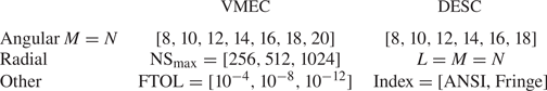
Additionally, the average normalized force error and time to solution for an aggregation of a number of DESC and VMEC solutions to the W7-X-like equilibrium run at a range of resolutions are shown in figure 12. The resolution scan ranges are shown in table 2. It is clear that for a given time to solution, DESC is able to achieve a lower average normalized force error than VMEC, indicating that DESC is able to achieve more accurate solutions than VMEC as measured by the force error metric. Often the DESC error is an order of magnitude lower than the VMEC error, as shown by the best-fit lines plotted in the figure. It should be noted that as DESC is written in Python, there is a certain amount of overhead associated with running the code versus a compiled Fortran code like VMEC. While the DESC code employs the JAX (Bradbury et al. Reference Bradbury, Frostig, Hawkins, Johnson, Leary, Maclaurin, Necula, Paszke, VanderPlas and Wanderman-Milne2018) package, which provides just-in-time compilation of code to improve performance, the code must first be called and compiled by JAX before the performance gains are seen. As such, the DESC solutions shown do not have runtimes lower than 2 minutes. However, pre-compilation is a planned future improvement to the JAX package, which will allow the DESC code to avoid costly just-in-time compilation during equilibrium solves, leading to lower initialization times.

Figure 12. Scatter plot of average force error versus runtime of W7-X finite-beta DESC and VMEC solutions at various resolutions, plotted along with linear fits of the results for each code. All calculations were run on the same hardware (32 GB RAM on a single AMD EPYC 7281 CPU). Note that for a given time to solution, DESC has generally an order-of-magnitude lower error, as seen by the best-fit lines for the results from each code.

Table 2. Solution parameters scanned over in obtaining the results shown in figure 12. Index refers to the spectral indexing scheme of the Zernike polynomials, which affects the radial resolution for a given $L$ and $M$ (Loomis Reference Loomis1978; Genberg et al. Reference Genberg, Michels and Doyle2002).

5.4. Mercier stability comparison

High-accuracy solutions to the MHD equilibrium equations are crucial for further analyses such as stability. This is well known in the tokamak community, where when solving the Grad–Shafranov equation for an equilibrium reconstruction, EFIT (Lao et al. Reference Lao, John, Stambaugh, Kellman and Pfeiffer1985) Picard iteration errors below $10^{-4}$ (Jiang et al. Reference Jiang, Sabbagh, Park, Berkery, Ahn, Riquezes, Bak, Ko, Ko and Lee2021; Xing et al. Reference Xing, Eldon, Nelson, Roelofs, Eggert, Izacard, Glasser, Logan, Meneghini and Smith2021) have been conventionally accepted as thresholds for reliable MHD stability analyses (Glasser Reference Glasser2016, Reference Glasser2020). These iteration error levels correspond to a similar magnitude of normalized (by the source terms) Grad–Shafranov force error. Note that the previously shown D-shaped tokamak equilibrium solved with DESC passes the required error threshold (in terms of normalized force error) of $10^{-4}$ as shown in figure 8, while the VMEC solution fails to meet this threshold even at high radial resolution, as shown in figure 7.

While no such rule of thumb exists for 3-D equilibria in the stellarator community, VMEC's inaccuracy near the magnetic axis has been found to cause issues when conducting ideal MHD stability analyses near the axis (A.H. Glasser, personal communication 2021).

As an example of higher-accuracy equilibria translating to more accurate stability calculations, the Mercier stability of a configuration described near equation (4.25) of the work by Landreman & Jorge (Reference Landreman and Jorge2020) is calculated, with the same equilibrium solved using the DESC and VMEC codes, and compared with asymptotic formulas from near-axis expansion theory from the same work. The internal routines from DESC are used to calculate its stability metrics, while for VMEC the $D_{{\rm Merc}}$ quantity that is calculated from its own internal routines and stored in its output file is used. The equilibrium is a finite-beta quasi-helically symmetric configuration with an aspect ratio of $\sim$20, and was solved in VMEC at two radial resolutions $ns=[65,801]$. The same equilibrium was also solved using DESC with radial resolution $L=12$ and ANSI spectral indexing. Both codes used a poloidal resolution of $M=12$ and a toroidal resolution of $N=10$. Instead of a fixed rotational transform profile, the equilibria were solved with a zero net toroidal current constraint in each code. The quasi-helical equilibrium used had the following pressure profile (given as a power series in $\rho = \sqrt {s} = \sqrt {{\psi }/{\psi _a}}$):

(5.6)\begin{equation} p(\rho) = 5000 - 5000 \rho^2\ ({\rm Pa}). \end{equation}

The pressure profile and the final rotational transform profile from the DESC equilibrium are plotted in figure 13, and the flux surfaces are shown in figure 14, which shows qualitative agreement in the equilibrium solution of the two codes. However, this qualitative agreement does not necessarily lead to quantitative agreement of stability metrics, as shown by the comparison of Mercier stability in this section. Mercier stability (Mercier Reference Mercier1964; Mercier & Luc Reference Mercier and Luc1974) is a measure of an ideal MHD equilibrium's stability to localized interchange perturbations about a rational surface, and the criterion for stability against such perturbations can be defined as (Bauer, Betancourt & Garabedian Reference Bauer, Betancourt and Garabedian1984)

(5.7)\begin{equation} D_{\text{Merc}}=D_{\text{Shear}}+D_{\text{Curr}}+D_{\text{Well}}+D_{\text{Geod}}>0, \end{equation}

where

(5.8a)\begin{gather} D_{\text{Shear}}=\frac{1}{16 {\rm \pi}^2}\left(\frac{\mathrm{d} \iota}{\mathrm{d} \psi}\right)^2, \end{gather}

(5.8b)\begin{gather}D_{\text{Curr}}={-}\frac{s_G}{(2 {\rm \pi})^4} \frac{\mathrm{d} \iota}{\mathrm{d} \psi} \int \,\mathrm{d} S \frac{\varXi \boldsymbol{\cdot} B}{|\boldsymbol{\nabla} \psi|^3}, \end{gather}

(5.8c)\begin{gather}D_{\text{Well}}=\left[\frac{\mu_0}{(2 {\rm \pi})^6} \frac{\mathrm{d} p}{\mathrm{d} \psi}\left(s_\psi \frac{\mathrm{d}^2 V}{\mathrm{d} \psi^2}-\mu_0 \frac{\mathrm{d} p}{\mathrm{d} \psi} \int \,\frac{\mathrm{d} S}{B^2|\boldsymbol{\nabla} \psi|} \right) \int \,\mathrm{d} S \frac{B^2}{|\boldsymbol{\nabla} \psi|^3}\right], \end{gather}

(5.8d)\begin{gather}D_{\mathrm{Geod}}=\left[\frac{1}{(2 {\rm \pi})^6}\left(\int \,\mathrm{d} S \frac{\mu_0 \boldsymbol{J} \boldsymbol{\cdot} \boldsymbol{B}}{|\boldsymbol{\boldsymbol{\nabla}} \psi|^3}\right)^2-\frac{1}{(2 {\rm \pi})^6}\left(\int \,\mathrm{d} S \frac{B^2}{|\boldsymbol{\nabla} \psi|^3}\right) \int \,\mathrm{d} S \frac{\left(\mu_0 \boldsymbol{J} \boldsymbol{\cdot} \boldsymbol{B}\right)^2}{B^2|\boldsymbol{\boldsymbol{\nabla}} \psi|^3}\right]. \end{gather}

Figure 13. Pressure and rotational transform profiles of the quasi-helical equilibrium DESC solution ($L=M=12$, $N=12$).

Figure 14. Flux surfaces for the VMEC ($ns=801$, $M=N=10$) and a DESC ($L=M=12$, $N=10$) quasi-helical equilibrium solution.

Here, $I(\psi )$ and $G(\psi )$ are the Boozer coordinate profile functions (Boozer Reference Boozer1981) and $s_g=\pm 1$ and $s_{\psi } = \pm 1$ are the signs of $G(\psi )$ and of the normalized toroidal flux $\psi$. Furthermore, $\varXi = \mu _0 \boldsymbol {J} - I'(\psi ) \boldsymbol {B}$, $V(\psi )$ is the volume enclosed by the flux surface labelled by $\psi$, and the surface integrals are taken over the given flux surface so that $dS = |\boldsymbol {\nabla } \psi \|\sqrt {g}|\,{\rm d}{\vartheta }\,{{\rm d}\varphi }$. The above equations were used to calculate Mercier stability of the equilibrium solutions from DESC and VMEC.

As a verification exercise, near-axis theory provides asymptotic expressions for the different components of Mercier stability that should match the full expressions above when $\epsilon = r/{R_{{\rm scale}}}$ is small, where here $R_{{\rm scale}} \sim {1}/{\kappa }$ is the scale length of the magnetic axis, $\kappa$ being the axis curvature, $r$ is the effective minor radius, $2{\rm \pi} \psi = {\rm \pi}r^2 \bar {B}$ and $\bar {B}$ is a constant reference magnetic field strength. Regardless of aspect ratio or scale length, the expansion is accurate close to the magnetic axis since $r \rightarrow 0$, and with higher aspect ratio the expansion becomes valid over a larger portion of the plasma volume. In Landreman & Jorge (Reference Landreman and Jorge2020) the asymptotic expressions for $D_{\mathrm {Geod}}$ and $D_{\text {Well}}$, the leading-order (in $\epsilon$) terms of $D_{{\rm Merc}}$, have been derived for quasi-symmetric equilibria:

(5.9)\begin{gather} D_{\text{Well}}=\frac{\mu_0 p_2\left|G_0\right|}{8 {\rm \pi}^4 r^2 B_0^3}\left[\frac{\mathrm{d}^2 V}{\mathrm{d} \psi^2}-\frac{8 {\rm \pi}^2 \mu_0 p_2\left|G_0\right|}{B_0^5}\right], \end{gather}

(5.10)\begin{gather}D_{\mathrm{Geod}}={-}\frac{2 \mu_0^2 p_2^2 G_0^4 \bar{\eta}^2}{{\rm \pi}^3 r^2 B_0^{10} \iota_{N 0}^2} \int_0^{2 {\rm \pi}}\, \mathrm{d} \varphi \frac{\bar{\eta}^4+\kappa^4 \sigma^2+\bar{\eta}^2 \kappa^2}{\bar{\eta}^4+\kappa^4\left(1+\sigma^2\right)+2 \bar{\eta}^2 \kappa^2}, \end{gather}

where (Landreman & Sengupta Reference Landreman and Sengupta2019) $G_0$ is the zeroth-order term of the expansion of the Boozer profile function $G$ in a power series in effective minor radius $r$, $B_0$ is the zeroth-order term in the power series expansion of the magnetic field strength $B$ in $r$, $p_2$ is the second-order term in the power series expansion of $p$ in $r$, $\bar {\eta }$ is a measure of the magnetic field strength variation, $\iota _{N0} = \iota _0 - N$, where $\iota _0$ is the zeroth-order term of the expansion of $\iota$ in $r$ and $N$ is a constant integer, and $\sigma$ is a solution to the ordinary differential equation defined in equation (2.14) of Landreman & Sengupta (Reference Landreman and Sengupta2019).

Thus to leading order, the Mercier stability of a quasi-symmetric stellarator calculated by the full expressions in (5.8) should agree with the sum of (5.9) and (5.10) at small $\epsilon$. Any deviation from agreement in a high-aspect-ratio equilibrium, especially near the magnetic axis, would then indicate an inaccuracy in the underlying equilibrium, as the calculated stability fails to agree with the asymptotic expression in the region where it is most valid.

Figure 15 shows $D_{{\rm Merc}}$ (made negative for the sake of plotting on a log scale, as the equilibrium is Mercier-unstable) of the two equilibria computed with VMEC in red, while that calculated from the DESC equilibrium is in cyan. Plotted as well is the value of $D_{{\rm Merc}}$ given by the asymptotic expressions. It can be seen that the stability computed from the DESC equilibrium agrees well with the asymptotic expression across the entirety of the plasma volume, but most importantly near the magnetic axis, indicating the equilibrium is sufficiently well resolved for accurate Mercier stability calculation. The VMEC equilibrium requires high radial resolution to agree with the asymptotic expression inside of $\rho < 0.5$, and even then differs from the asymptotic value nearer to the magnetic axis, indicating a failure to accurately satisfy the ideal MHD equilibrium equations there. Upon inspection of the individual terms in the $D_{{\rm Merc}}$ sum, the $D_{{\rm Geod}}$ term is the most significant part of $D_{{\rm Merc}}$ in the core of the equilibrium, and it is this dominant term which is responsible for the large deviation in $D_{{\rm Merc}}$ from the asymptotically derived values near the axis. The lack of convergence of $D_{{\rm Geod}}$ in VMEC with increasing resolution has been seen by previous work (Landreman & Jorge Reference Landreman and Jorge2020). This deviation is roughly correlated with the radial position where the force error in each VMEC solution begins to increase sharply nearing the axis, shown in figure 16.

Figure 15. Mercier stability calculated from VMEC equilibria of increasing radial resolution, as compared with a DESC equilibrium of $L=12$. Both codes were run with toroidal resolution of $N=10$ and poloidal resolution of $M=12$. The DESC solution compares much better with the asymptotic value of $D_{{\rm Merc}}$ near the axis, while the VMEC solution even with high resolution fails to resolve the stability near the axis.

Figure 16. Normalized force error flux-surface average of the VMEC and DESC equilibria corresponding to the calculations in figure 15.

One possible explanation for such a difference in accuracy between the DESC and VMEC solutions is that DESC's 3-D spectral basis results in more accurate radial derivatives as compared with VMEC's finite differencing. Of the two leading-order terms in $D_{{\rm Merc}}$ near the axis, the $D_{{\rm Geod}}$ term requires higher-order radial derivatives of the coordinates $R,Z$, due to the presence of the current density $\boldsymbol {J}$ in the expression. So, an inaccuracy in the radial derivatives would most strongly affect this term, leading to the lack of agreement with the asymptotic result at the axis. This inaccuracy in radial derivatives also manifests itself in worse force error. This shows the importance of accurate equilibria, especially near the axis, as VMEC's lack of accuracy leads to disagreement with asymptotic theory in the region where the theory is most valid, while DESC's accurate treatment of the axis results in accurate Mercier stability calculations as well.

6. Conclusions

In conclusion, a comparison of the VMEC and DESC codes was carried out. DESC was shown to have more accurate equilibrium solutions than VMEC as measured by force balance error, and to have faster runtimes for a given solution accuracy. DESC was also shown to have improved radial convergence as compared with VMEC, owing to its spectral basis in all three coordinates. Further, inaccuracies of VMEC solutions near the axis were seen, which could be tied to the unphysical modes in the VMEC Fourier spectrum that do not scale correctly with radius near the axis. DESC solutions, on the other hand, do not have this problem, and were shown to be accurate near the axis. Solution accuracy is necessary in order to accurately calculate stability metrics, and this is explicitly shown for a Mercier stability calculation, where the DESC solution is found to better agree with the asymptotic expansion near the axis than the VMEC solution. Future plans for development of the DESC code with regards to computation speed include implementing message passing interface parallelization to better take advantage of CPUs and benchmarking the code's graphics processing unit (GPU) capabilities. Pre-compilation of functions with JAX is also foreseen, which should aid in reducing initialization times. Additionally, further DESC verification can include comparing results with other equilibrium codes such as SPEC, and the effect of solution accuracy can be investigated in other metrics such as fast particle confinement.

Acknowledgements

The authors gratefully acknowledge helpful discussions with Matt Landreman concerning near-axis expansion theory and Mercier stability.

Editor Per Helander thanks the referees for their advice in evaluating this article.

Funding

This work was supported by the US Department of Energy under contract numbers DE-AC02-09CH11466 and DE-SC0022005 and Field Work Proposal No. 1019. The United States Government retains a non-exclusive, paid-up, irrevocable, world-wide licence to publish or reproduce the published form of this paper, or allow others to do so, for United States Government purposes.

Declaration of interests

The authors report no conflict of interest.

Data availability statement

The data and scripts used in this paper are freely available on Zenodo (Panici Reference Panici2022) at https://doi.org/10.5281/zenodo.6539680.

Appendix A. Force balance error from VMEC $R,Z,\lambda$ Fourier coefficients

With the cylindrical coordinate system $\boldsymbol {x} = (R,\phi,Z)$, VMEC uses as its computational coordinates $\boldsymbol {\alpha } = (s,u,v)$, with $s$ being a radial coordinate proportional to the normalized toroidal flux, $u$ a poloidal-like angle and $v$ is the geometric toroidal angle for one field period:

(A1a)\begin{gather} s = \frac{\psi}{\psi_a} ,\quad 0\leq s \leq 1, \end{gather}

(A1b)\begin{gather} u = \theta^* - \lambda(s,u,v),\quad 0\leq u \leq 2{\rm \pi}, \end{gather}

(A1c)\begin{gather} v = \phi ,\quad 0\leq v \leq \frac{2{\rm \pi}}{N_{FP}}, \end{gather}

where $\psi _a$ is the toroidal flux enclosed by the plasma boundary (at $s=1$) that is normalized by $2{\rm \pi}$, $\lambda (s,u,v)$ is a function periodic in $(u,v)$ that converts $u$ to a straight-field-line poloidal angle $\theta ^*$, $N_{FP}$ is the number of field periods in the device and $\phi$ is the usual geometric toroidal angle coordinate.

The covariant basis vectors $\boldsymbol {e}_{i} = {\partial \boldsymbol {x}}/{\partial \alpha _i}$ for the $\alpha =(s,u,v)$ coordinate system are

(A2a)\begin{gather} {\boldsymbol e}_{s} = \begin{bmatrix} \partial_{s}R \\ 0 \\ \partial_{s}Z \end{bmatrix}, \end{gather}

(A2b)\begin{gather} {\boldsymbol e}_{u} = \begin{bmatrix} \partial_{u}R \\ 0 \\ \partial_{u}Z \end{bmatrix}, \end{gather}

(A2c)\begin{gather} {\boldsymbol e}_{v} = \begin{bmatrix} \partial_{v}R \\ R \\ \partial_{v}Z \end{bmatrix}, \end{gather}

and the notation ${\boldsymbol e}_{\alpha \gamma }$ is used as a shorthand for $\partial _\gamma ( {\boldsymbol e}_{\alpha } )$. The Jacobian and its partial derivatives are calculated from the basis vectors as

(A3a)\begin{gather} \sqrt{g} = {\boldsymbol e}_{s}\boldsymbol{\cdot}{\boldsymbol e}_{u}\times{\boldsymbol e}_{v} , \end{gather}

(A3b)\begin{gather}\partial_s \left(\sqrt{g}\right) = {\boldsymbol e}_{ss}\boldsymbol{\cdot}{\boldsymbol e}_{u}\times{\boldsymbol e}_{v} + {\boldsymbol e}_{s}\boldsymbol{\cdot}{\boldsymbol e}_{us}\times{\boldsymbol e}_{v} + {\boldsymbol e}_{s}\boldsymbol{\cdot}{\boldsymbol e}_{u}\times{\boldsymbol e}_{vs}, \end{gather}

(A3c)\begin{gather}\partial_u \left(\sqrt{g}\right) = {\boldsymbol e}_{su}\boldsymbol{\cdot}{\boldsymbol e}_{u}\times{\boldsymbol e}_{v} + {\boldsymbol e}_{s}\boldsymbol{\cdot}{\boldsymbol e}_{uu}\times{\boldsymbol e}_{v} + {\boldsymbol e}_{s}\boldsymbol{\cdot}{\boldsymbol e}_{u}\times{\boldsymbol e}_{vu}, \end{gather}

(A3d)\begin{gather}\partial_v \left(\sqrt{g}\right) = {\boldsymbol e}_{sv}\boldsymbol{\cdot}{\boldsymbol e}_{u}\times{\boldsymbol e}_{v} + {\boldsymbol e}_{s}\boldsymbol{\cdot}{\boldsymbol e}_{uv}\times{\boldsymbol e}_{v} + {\boldsymbol e}_{s}\boldsymbol{\cdot}{\boldsymbol e}_{u}\times{\boldsymbol e}_{vv}. \end{gather}

Contravariant basis vectors $\boldsymbol {e}^{i} = \boldsymbol {\nabla }\alpha _i$ are given by

(A4a)\begin{gather} {\boldsymbol e}^{s} = \frac{{\boldsymbol e}_{u} \times {\boldsymbol e}_{v}}{\sqrt{g}}, \end{gather}

(A4b)\begin{gather}{\boldsymbol e}^{u} = \frac{{\boldsymbol e}_{v} \times {\boldsymbol e}_{s}}{\sqrt{g}}, \end{gather}

(A4c)\begin{gather}{\boldsymbol e}^{v} = \frac{{\boldsymbol e}_{s} \times {\boldsymbol e}_{u}}{\sqrt{g}}. \end{gather}

The metric tensor components are given by

(A5a)\begin{gather} g^{ss}= {\boldsymbol e}^{s}\boldsymbol{\cdot}{\boldsymbol e}^{s} , \end{gather}

(A5b)\begin{gather}g^{vv} = {\boldsymbol e}^{v}\boldsymbol{\cdot}{\boldsymbol e}^{v} , \end{gather}

(A5c)\begin{gather}g^{uu} = {\boldsymbol e}^{u}\boldsymbol{\cdot}{\boldsymbol e}^{u} , \end{gather}

(A5d)\begin{gather}g^{uv} = {\boldsymbol e}^{u}\boldsymbol{\cdot}{\boldsymbol e}^{v}. \end{gather}

Recall that the magnetic field can be written in the form

(A6a)\begin{align} \boldsymbol{B} & = B_s {\boldsymbol e}^{s} + B_u {\boldsymbol e}^{u} + B_v {\boldsymbol e}^{v} \end{align}

(A6b)\begin{align} & = B^u {\boldsymbol e}_{u} + B^v {\boldsymbol e}_{v} \end{align}

and that in the VMEC coordinate system the contravariant components of the field are given by (Hirshman & Whitson Reference Hirshman and Whitson1983, p. 3)

(A7a)\begin{gather} B^u = \frac{1}{\sqrt{g}} \left(\chi' - \psi' \dfrac{\partial\lambda}{\partial v} \right), \end{gather}

(A7b)\begin{gather}B^v = \frac{1}{\sqrt{g}} \psi'\left(1 + \dfrac{\partial\lambda}{\partial u} \right), \end{gather}

where $2{\rm \pi} \chi (s)$ and $2{\rm \pi} \psi (s)$ are the poloidal and toroidal magnetic fluxes, respectively, the prime denotes a radial derivative $\partial / \partial s$ and $\lambda$ is a function periodic in $u,v$ with zero average over a magnetic surface, $\iint \,{\rm d}u\,{\rm d}v\lambda = 0$.

The MHD force balance equilibrium is given by

(A8a)\begin{gather} \boldsymbol{F} ={-}\boldsymbol{J} \times \boldsymbol{B} + \boldsymbol{\nabla} p = 0, \end{gather}

(A8b)\begin{gather}\boldsymbol{\nabla} \times \boldsymbol{B} = \mu_0 \boldsymbol{J}, \end{gather}

(A8c)\begin{gather}\boldsymbol{\nabla} \boldsymbol{\cdot} \boldsymbol{B} = 0. \end{gather}

The magnetic field can be written as

(A9a)\begin{align} \boldsymbol{B} & = \boldsymbol{\nabla} v \times \boldsymbol{\nabla} \chi + \boldsymbol{\nabla} \psi \times \boldsymbol{\nabla} \theta^* \end{align}

(A9b)\begin{align} & = B^u {\boldsymbol e}_{u} + B^v {\boldsymbol e}_{v}, \end{align}

where $\theta ^* = u + \lambda (s,u,v)$ is a straight-field-line poloidal angle. Inserting (A9a) into (A8a) yields

(A10)\begin{equation} \boldsymbol{F} = F_s \boldsymbol{\nabla} s + F_{\beta} \boldsymbol{\beta}, \end{equation}

where

(A11a)\begin{gather} F_s = \sqrt{g}(J^vB^u - J^uB^v) + p', \end{gather}

(A11b)\begin{gather}F_{\beta} = J^s, \end{gather}

where $\beta = \sqrt {g}(B^v \boldsymbol {\nabla } u - B^u \boldsymbol {\nabla } v)$ and $J^i = \boldsymbol {J} \boldsymbol {\cdot } \boldsymbol {\nabla } \alpha _i = \mu _0^{-1} \boldsymbol {\nabla } \boldsymbol {\cdot } (\boldsymbol {B} \times \boldsymbol {\nabla } \alpha _i)$.

Contravariant components of $\boldsymbol {J}$ can be written with the derivatives of covariant $B$ components $\boldsymbol {B} = B_i e^i$:

(A12a)\begin{gather} J^s = \mu_0^{{-}1} \boldsymbol{\nabla} \boldsymbol{\cdot} (\boldsymbol{B} \times \boldsymbol{\nabla} s) = \frac{1}{\mu_0 \sqrt{g}} \boldsymbol{\nabla} \boldsymbol{\cdot} (B_v \boldsymbol{\nabla} u - B_u \boldsymbol{\nabla} v), \end{gather}

(A12b)\begin{gather}J^s= \frac{1}{\mu_0 \sqrt{g}}\left(\frac{\partial B_v}{\partial u} - \frac{\partial B_u}{\partial v}\right) = F_{\beta}, \end{gather}

(A12c)\begin{gather}J^u = \mu_0^{{-}1} \boldsymbol{\nabla} \boldsymbol{\cdot} (\boldsymbol{B} \times \boldsymbol{\nabla} u) = \frac{1}{\mu_0 \sqrt{g}} \boldsymbol{\nabla} \boldsymbol{\cdot} ({-}B_v \boldsymbol{\nabla} s + B_s \boldsymbol{\nabla} v), \end{gather}

(A12d)\begin{gather}J^u= \frac{1}{\mu_0 \sqrt{g}}\left(\frac{\partial B_s}{\partial v} - \frac{\partial B_v}{\partial s}\right), \end{gather}

(A12e)\begin{gather}J^v = \mu_0^{{-}1} \boldsymbol{\nabla} \boldsymbol{\cdot} (\boldsymbol{B} \times \boldsymbol{\nabla} v) = \frac{1}{\mu_0 \sqrt{g}} \boldsymbol{\nabla} \boldsymbol{\cdot} (B_u \boldsymbol{\nabla} s - B_s \boldsymbol{\nabla} u), \end{gather}

(A12f)\begin{gather}J^v = \frac{1}{\mu_0 \sqrt{g}}\left(\frac{\partial B_u}{\partial s} - \frac{\partial B_s}{\partial u}\right). \end{gather}

The covariant components of $B$ are

(A13a)\begin{gather} B_s = \boldsymbol{B} \boldsymbol{\cdot} {\boldsymbol e}_{s} = (B^u {\boldsymbol e}_{u} + B^v {\boldsymbol e}_{v}) \boldsymbol{\cdot} {\boldsymbol e}_{s}, \end{gather}

(A13b)\begin{gather}B_u = \boldsymbol{B} \boldsymbol{\cdot} {\boldsymbol e}_{u} = (B^u {\boldsymbol e}_{u} + B^v {\boldsymbol e}_{v}) \boldsymbol{\cdot} {\boldsymbol e}_{u}, \end{gather}

(A13c)\begin{gather}B_v = \boldsymbol{B} \boldsymbol{\cdot} {\boldsymbol e}_{v} = (B^u {\boldsymbol e}_{u} + B^v {\boldsymbol e}_{v}) \boldsymbol{\cdot} {\boldsymbol e}_{v}. \end{gather}

The partial derivatives of the contravariant components of $B$ are for $B^u$

(A14a)\begin{gather} \partial_s B^u ={-}\frac{\partial_s(\sqrt{g})}{g} \left(\chi'-\psi'\dfrac{\partial\lambda}{\partial v}\right) + \frac{1}{\sqrt{g}} \left(\chi'' - \psi''\dfrac{\partial\lambda}{\partial v} - \psi' \dfrac{\partial^2\lambda}{\partial s \partial v }\right), \end{gather}

(A14b)\begin{gather}\partial_u B^u ={-}\frac{\partial_u(\sqrt{g})}{g} \left(\chi'-\psi'\dfrac{\partial\lambda}{\partial v}\right) + \frac{1}{\sqrt{g}} \left(- \psi' \dfrac{\partial^2\lambda}{\partial u \partial v }\right), \end{gather}

(A14c)\begin{gather}\partial_v B^u ={-}\frac{\partial_v(\sqrt{g})}{g} \left(\chi'-\psi'\dfrac{\partial\lambda}{\partial v} \right) + \frac{1}{\sqrt{g}} \left(- \psi' \dfrac{\partial^2\lambda}{\partial v^2 } \right) \end{gather}

and for $B^v$

(A15a)\begin{gather} \partial_s B^v = \left(-\frac{\partial_s(\sqrt{g})}{g} \psi' + \frac{\psi''}{\sqrt{g}}\right)\left(1+\dfrac{\partial\lambda}{\partial u}\right) + \frac{\psi'}{\sqrt{g}}\left(\dfrac{\partial^2\lambda}{\partial s \partial u }\right), \end{gather}

(A15b)\begin{gather}\partial_u B^v ={-}\frac{\partial_u(\sqrt{g})}{g} \psi' \left(1+\dfrac{\partial\lambda}{\partial u}\right) + \frac{\psi'}{\sqrt{g}}\left(\dfrac{\partial^2\lambda}{\partial u^2 }\right), \end{gather}

(A15c)\begin{gather}\partial_v B^v ={-}\frac{\partial_v(\sqrt{g})}{g} \psi' \left(1+\dfrac{\partial\lambda}{\partial u}\right) + \frac{\psi'}{\sqrt{g}}\left(\dfrac{\partial^2\lambda}{\partial u \partial v }\right). \end{gather}

With these defined, and using (A13), the partial derivatives of the covariant components of $B$ are then

(A16a)\begin{gather} {\partial_{s}B_{u} = \left(\partial_{s}B^u{\boldsymbol e}_{u} + B^u\boldsymbol{e}_{us} + \partial_{s}B^v{\boldsymbol e}_{v} + B^v\boldsymbol{e}_{vs}\right)\boldsymbol{\cdot} \boldsymbol{e}_{u} + \left(B^u{\boldsymbol e}_{u} + B^v{\boldsymbol e}_{v} \right)\boldsymbol{\cdot} \boldsymbol{e}_{u s}}, \end{gather}

(A16b)\begin{gather} {\partial_{s}B_{v} = \left(\partial_{s}B^u{\boldsymbol e}_{u} + B^u\boldsymbol{e}_{us} + \partial_{s}B^v{\boldsymbol e}_{v} + B^v\boldsymbol{e}_{vs}\right)\boldsymbol{\cdot} \boldsymbol{e}_{v} + \left(B^u{\boldsymbol e}_{u} + B^v{\boldsymbol e}_{v} \right)\boldsymbol{\cdot} \boldsymbol{e}_{v s}}, \end{gather}

(A16c)\begin{gather} {\partial_{u}B_{s} = \left(\partial_{u}B^u{\boldsymbol e}_{u} + B^u\boldsymbol{e}_{uu} + \partial_{u}B^v{\boldsymbol e}_{v} + B^v\boldsymbol{e}_{vu}\right)\boldsymbol{\cdot} \boldsymbol{e}_{s} + \left(B^u{\boldsymbol e}_{u} + B^v{\boldsymbol e}_{v} \right)\boldsymbol{\cdot} \boldsymbol{e}_{s u}}, \end{gather}

(A16d)\begin{gather} {\partial_{u}B_{v} = \left(\partial_{u}B^u{\boldsymbol e}_{u} + B^u\boldsymbol{e}_{uu} + \partial_{u}B^v{\boldsymbol e}_{v} + B^v\boldsymbol{e}_{vu}\right)\boldsymbol{\cdot} \boldsymbol{e}_{v} + \left(B^u{\boldsymbol e}_{u} + B^v{\boldsymbol e}_{v} \right)\boldsymbol{\cdot} \boldsymbol{e}_{v u}}, \end{gather}

(A16e)\begin{gather} {\partial_{v}B_{s} = \left(\partial_{v}B^u{\boldsymbol e}_{u} + B^u\boldsymbol{e}_{uv} + \partial_{v}B^v{\boldsymbol e}_{v} + B^v\boldsymbol{e}_{vv}\right)\boldsymbol{\cdot} \boldsymbol{e}_{s} + \left(B^u{\boldsymbol e}_{u} + B^v{\boldsymbol e}_{v} \right)\boldsymbol{\cdot} \boldsymbol{e}_{s v}}, \end{gather}

(A16f)\begin{gather} {\partial_{v}B_{u} = \left(\partial_{v}B^u{\boldsymbol e}_{u} + B^u\boldsymbol{e}_{uv} + \partial_{v}B^v{\boldsymbol e}_{v} + B^v\boldsymbol{e}_{vv}\right)\boldsymbol{\cdot} \boldsymbol{e}_{u} + \left(B^u{\boldsymbol e}_{u} + B^v{\boldsymbol e}_{v} \right)\boldsymbol{\cdot} \boldsymbol{e}_{u v}}. \end{gather}

With these, all of the required derivatives to evaluate the force components $F_s$ and $F_\beta$ are known. The magnitudes of the directions of each component are

(A17a)\begin{align} \|\boldsymbol{\nabla} s\|_2 & = \sqrt{{\boldsymbol e}^{s} \boldsymbol{\cdot} {\boldsymbol e}^{s}} = \sqrt{g^{ss}}, \end{align}

(A17b)\begin{align} \|\boldsymbol{\beta}\|_2 & = \|\sqrt{g}\left(B^v{\boldsymbol e}^{u} - B^u {\boldsymbol e}^{v}\right)\|_2 \end{align}

(A17c)\begin{align} & = \sqrt{g}\sqrt{(B^v)^2g^{uu} + (B^u)^2g^{vv} - 2B^vB^ug^{uv}}. \end{align}

The magnitude of force balance error is then

(A18)\begin{equation} \|\boldsymbol{F}\|_2 = \sqrt{\left(F_s\right)^2g^{ss} + \left(F_{\beta}\right)^2 \left(\|\boldsymbol{\beta}\|_2\right)^2}. \end{equation}

Now $R$, $Z$ and $\lambda$ are explicitly known analytically only in $u,v$ on discrete flux surfaces on the radial grid $s$. Function $\lambda$ also is calculated on a half-mesh offset from the main radial grid, and must be interpolated onto the main radial grid first. So, numerical derivatives are used for all of the radial derivatives $\partial _s$ of $R$, $Z$ and $\lambda$ necessary to calculate $\boldsymbol {F}$. The derivatives are carried out on the Fourier coefficients RMNC, ZMNS and LMNS (to get the Fourier coefficients of the derivatives, e.g. ${\partial {\rm RMNC}}/{\partial s}|_{s_i} = {\rm RSMNC} = ({{\rm RMNC}(s_{i+1}) -{\rm RMNC}(s_{i})})/{\Delta s}$).

Appendix B. VMEC force error spikes

In the W7-X finite-beta equilibria computed here, spikes are observed in the calculated force error flux-surface average.

These spikes correspond to discontinuous jumps in the radial derivatives of the Fourier coefficients for $R,Z$, shown in figures 17 and 18 for the $m=3,n=1$ mode of $R_{mnc}$ (chosen only as a representative example; this is seen in other mode numbers as well). Note that these spikes do not correspond to any low-order rationals, plotted in figure 18, so they do not stem from current singularities at rational surfaces. This is further supported by the parallel current density not exhibiting singular behaviour at the rational surfaces plotted, shown in figure 3. Plotted are all rationals $N/M$ in the ranges $M=(1,19),~N=(1,18)$ that lie in the iota profile (the profile is plotted in figure 1).

Figure 17. First radial derivative of RMNC $m=3$ $n=1$ coefficient (found with finite differences) for W7-X $M=N=16$ with $ns=512$.

Figure 18. Second radial derivative of RMNC $m=3$ $n=1$ coefficient (found with finite differences) for W7-X $M=N=16$ with $ns=512$.

Running the same equilibrium with higher solver tolerances (shown in figure 19) and with higher angular resolution (such as in figure 20) does not completely eliminate these spikes. Increasing the FTOL parameter past $1\times 10^{-14}$ resulted in the equilibrium solve taking prohibitively long (longer than 24 h when run with 32 GB RAM on a single AMD EPYC 7281 CPU), so the tolerance scan at ${\rm NS}=1024$, $M=N=16$ was not carried out past ${\rm FTOL}=1\times 10^{-14}$.

Figure 19. The W7-X flux-surface average of normalized force error versus $\rho$ for increasingly tighter solver tolerance (all with angular resolution of $M=N=16$ and ${\rm NS}=1024$ flux surfaces). Second-order finite differences were used as the radial derivative in calculating the force error.

Figure 20. The W7-X flux-surface average of normalized force error versus $\rho$ for increasing VMEC angular resolution (all with radial resolution of ${\rm NS}=1024$). Second-order finite differences were used as the radial derivative in calculating the force error.

Appendix C. VMEC and DESC convergence scans

In computing solutions for the comparison in this paper, convergence scans were carried out with each code, the results of which are compiled here. In figure 21, the results for running VMEC at an angular resolution of $M=N=16$ (512 Fourier modes per surface) for increasing number of radial surfaces are shown. It can be seen that after ${\rm NS}=1024$, the normalized force error does not decrease appreciably across most of the volume, and the spikes in error near the edge become much more pronounced with ${\rm NS}=2048$.

Figure 21. The W7-X flux-surface average of normalized force error versus $\rho$ for increasing VMEC radial resolution (all with angular resolution of $M=N=16$). The force error does not decrease appreciably past 1024 surfaces for most of the plasma volume, and the error spikes near the edge increase in size as NS increases. Second-order finite differences were used as the radial derivative in calculating the force error.

Next, a scan over angular resolution was carried out in VMEC, and shown in figure 20. The force error is seen to decrease with increasing angular resolution across the whole volume until $M=N=20$, where it begins to stagnate and not uniformly decrease. A similar scan was carried out in DESC, and shown in figure 22. In DESC, due to the Fourier–Zernike basis, the poloidal and radial modes are coupled, so increasing the poloidal resolution $M$ also increases the radial resolution $L$. It can be seen that around $L=M=N=16$, the normalized force error begins to not decrease uniformly across the plasma volume. The minima in the force error flux-surface averages here correspond to collocation points.

Figure 22. The W7-X flux-surface average of normalized force error versus $\rho$ for increasing DESC angular and radial resolution. The ANSI Zernike indexing pattern was used (Dudt & Kolemen Reference Dudt and Kolemen2020).

Among the parameters scanned over for the VMEC solutions shown in this paper was the FTOL solver tolerance parameter. Shown in figure 23 are results of running the W7-X-like equilibrium at different angular and radial resolutions, and at a range of FTOL values. It can be seen that at low angular resolutions (lower than the boundary Fourier series resolution of $M=N=12$), the FTOL parameter does not affect the solution accuracy much. This is likely because the limiting factor in the solution accuracy is the low angular resolution being unable to match the flux surfaces to the boundary Fourier series. At higher angular resolutions, it can be seen that the FTOL parameter being too low limits the accuracy of the solution, as expected as it terminates the solver prematurely. The difference in the solutions found using ${\rm FTOL}=1\times 10^{-8}$ and ${\rm FTOL}=1\times 10^{-12}$ becomes larger as the angular resolution of the solution is increased.

Figure 23. VMEC results labelled with FTOL, showing that low FTOL results in stagnation in error decrease with increasing resolution, as expected.

References

Bañón Navarro, A., Merlo, G., Plunk, G.G., Xanthopoulos, P., von Stechow, A., Di Siena, A., Maurer, M., Hindenlang, F., Wilms, F. & Jenko, F. 2020 Global gyrokinetic simulations of ITG turbulence in the magnetic configuration space of the Wendelstein 7-X stellarator. Plasma Phys. Control. Fusion 62 (10), 105005.CrossRef Google Scholar

Bauer, F., Betancourt, O. & Garabedian, P. 1978 A Computational Method in Plasma Physics. Springer.CrossRef Google Scholar

Bauer, F., Betancourt, O. & Garabedian, P. 1984 Magnetohydrodynamic Equilibrium and Stability of Stellarators. Springer.CrossRef Google Scholar

Betancourt, O. 1988 BETAS: a spectral code for three-dimensional magnetohydrodynamic equilibrium and nonlinear stability calculations. Commun. Pure Appl. Maths 41 (5), 551–568.CrossRef Google Scholar

Betancourt, O. & Garabedian, P. 1976 Equilibrium and stability code for a diffuse plasma. Proc. Natl Acad. Sci. 73 (4), 984–987.CrossRef Google Scholar PubMed

Bhattacharjee, A., Wiley, J.C. & Dewar, R.L. 1984 Variational method for three-dimensional toroidal equilibria. Comput. Phys. Commun. 31 (2), 213–225.CrossRef Google Scholar

Boozer, A.H. 1981 Plasma equilibrium with rational magnetic surfaces. Phys. Fluids 24 (11), 1999–2003.CrossRef Google Scholar

Boyd, J.P. 2001 Chebyshev and Fourier Spectral Methods: Second Revised Edition. Courier Corporation.Google Scholar

Bradbury, J., Frostig, R., Hawkins, P., Johnson, M.J., Leary, C., Maclaurin, D., Necula, G., Paszke, A., VanderPlas, J., Wanderman-Milne, S., et al. 2018 JAX: composable transformations of Python+NumPy programs, version 0.3.13. http://github.com/google/jax.Google Scholar

Cerfon, A.J. & Freidberg, J.P. 2010 “One size fits all” analytic solutions to the Grad–Shafranov equation. Phys. Plasmas 17 (3), 032502.CrossRef Google Scholar

Chodura, R. & Schlüter, A. 1981 A 3D code for MHD equilibrium and stability. J. Comput. Phys. 41 (1), 68–88.CrossRef Google Scholar

Collatz, L. 1960 The Numerical Treatment of Differential Equations. Springer.Google Scholar

Conlin, R., Dudt, D.W., Panici, D. & Kolemen, E. 2023 The DESC stellarator code suite part II: Perturbation and continuation methods. J. Plasma Phys. Submitted. arXiv:2203.15927.Google Scholar

Drevlak, M., Beidler, C.D., Geiger, J., Helander, P. & Turkin, Y. 2019 Optimisation of stellarator equilibria with rose. Nucl. Fusion 59 (1), 016010.CrossRef Google Scholar

Dudt, D., Conlin, R., Panici, D. & Kolemen, E. 2023 The DESC stellarator code suite Part 3: Quasi-symmetry optimization. J. Plasma Phys. 89 (2), 955890201. doi:10.1017/S0022377823000235.CrossRef Google Scholar

Dudt, D.W., Conlin, W., Panici, D., Unalmis, K., Kim, P. & Kolemen, E. 2022 DESC. https://github.com/PlasmaControl/DESC.Google Scholar

Dudt, D.W. & Kolemen, E. 2020 DESC: a stellarator equilibrium solver. Phys. Plasmas 27 (10), 102513.CrossRef Google Scholar

Genberg, V.L., Michels, G.J. & Doyle, K.B. 2002 Orthogonality of zernike polynomials. Proc. SPIE 4771, 276–286.CrossRef Google Scholar

Glasser, A.H. 2016 The direct criterion of Newcomb for the ideal MHD stability of an axisymmetric toroidal plasma. Phys. Plasmas 23, 72505.CrossRef Google Scholar

Glasser, A.H. 2020 The direct criterion of Newcomb for the ideal MHD stability of stepped-pressure stellarators. Phys. Plasmas 27 (4), 042509.CrossRef Google Scholar

Guazzotto, L. & Freidberg, J.P. 2021 Simple, general, realistic, robust, analytic tokamak equilibria. Part 1. Limiter and divertor tokamaks. J. Plasma Phys. 87 (3), 905870303.CrossRef Google Scholar

Helander, P. 2014 Theory of plasma confinement in non-axisymmetric magnetic fields. Rep. Prog. Phys. 77 (8), 087001.CrossRef Google Scholar PubMed

Hender, T.C., Carreras, B.A., Garcia, L., Rome, J.A. & Lynch, V.E. 1985 The calculation of stellarator equilibria in vacuum flux surface coordinates. J. Comput. Phys. 60 (1), 76–96.CrossRef Google Scholar

Hirshman, S.P. & Breslau, J. 1998 Explicit spectrally optimized Fourier series for nested magnetic surfaces. Phys. Plasmas 5 (7), 2664–2675.CrossRef Google Scholar

Hirshman, S.P., Sanchez, R. & Cook, C.R. 2011 SIESTA: a scalable iterative equilibrium solver for toroidal applications. Phys. Plasmas 18 (6), 062504.CrossRef Google Scholar

Hirshman, S.P. & Whitson, J.C. 1983 Steepest-descent moment method for three-dimensional magnetohydrodynamic equilibria. Phys. Fluids 26 (12), 3553–3568.CrossRef Google Scholar

Hudson, S.R., Dewar, R.L., Dennis, G., Hole, M.J., McGann, M., von Nessi, G. & Lazerson, S. 2012 Computation of multi-region relaxed magnetohydrodynamic equilibria. Phys. Plasmas 19 (11), 112502.CrossRef Google Scholar

Hudson, S.R., Loizu, J., Zhu, C., Qu, Z.S., Nührenberg, C., Lazerson, S., Smiet, C.B. & Hole, M.J. 2020 Free-boundary MRxMHD equilibrium calculations using the stepped-pressure equilibrium code. Plasma Phys. Control. Fusion 62 (8), 084002.CrossRef Google Scholar

Jiang, Y., Sabbagh, S.A., Park, Y.S., Berkery, J.W., Ahn, J.H., Riquezes, J.D., Bak, J.G., Ko, W.H., Ko, J., Lee, J.H., et al. 2021 Kinetic equilibrium reconstruction and the impact on stability analysis of KSTAR plasmas. Nucl. Fusion 61 (11), 116033.CrossRef Google Scholar

Kruskal, M.D. & Kulsrud, R.M. 1958 Equilibrium of a magnetically confined plasma in a toroid. Phys. Fluids 1 (4), 265–274.CrossRef Google Scholar

Landreman, M. & Jorge, R. 2020 Magnetic well and Mercier stability of stellarators near the magnetic axis. J. Plasma Phys. 86 (5), 905860510.CrossRef Google Scholar

Landreman, M., Medasani, B., Wechsung, F., Giuliani, A., Jorge, R. & Zhu, C. 2021 Simsopt: a flexible framework for stellarator optimization. J. Open Source Softw. 6 (65), 3525.CrossRef Google Scholar

Landreman, M. & Sengupta, W. 2019 Constructing stellarators with quasisymmetry to high order. J. Plasma Phys. 85 (6), 815850601.CrossRef Google Scholar

Lao, L.L., John, H.S., Stambaugh, R.D., Kellman, A.G. & Pfeiffer, W. 1985 Reconstruction of current profile parameters and plasma shapes in tokamaks. Nucl. Fusion 25 (11), 1611–1622.CrossRef Google Scholar

Lazerson, S., Schmitt, J., Zhu, C., Breslau, J., All STELLOPT Developers & USDOE Office of Science 2020 Stellopt, version 2.7.5.Google Scholar

Lewis, H.R. & Bellan, P.M. 1990 Physical constraints on the coefficients of Fourier expansions in cylindrical coordinates. J. Math. Phys. 31 (11), 2592–2596.CrossRef Google Scholar

Loomis, J. 1978 A computer program for analysis of interferometric data. ASTM STP 666, 71–86.Google Scholar

Mercier, C. 1964 Equilibrium and stability of a toroidal magnetohydrodynamic system in the neighbourhood of a magnetic axis. Nucl. Fusion 4 (3), 213–226.CrossRef Google Scholar

Mercier, C. & Luc, H. 1974 The Magnetohydrodynamic Approach to the Problem of Plasma Confinement in Closed Magnetic Configurations. Commission of the European Communities.Google Scholar

Panici, D. 2022 Dataset on Zenodo. Inputs and outputs for paper the DESC stellarator code suite part I: quick and accurate equilibria computations. Available at: https://doi.org/10.5281/zenodo.6539680.CrossRef Google Scholar

Press, W.H., ed. 1996 Numerical recipes in Pascal. Book: William H. Press, repr edn. Cambridge University Press.Google Scholar

Qu, Z.S., Pfefferlé, D., Hudson, S.R., Baillod, A., Kumar, A., Dewar, R.L. & Hole, M.J. 2020 Coordinate parameterisation and spectral method optimisation for Beltrami field solver in stellarator geometry. Plasma Phys. Control. Fusion 62 (12), 124004.CrossRef Google Scholar

Reiman, A. & Greenside, H. 1986 Calculation of three-dimensional MHD equilibria with islands and stochastic regions. Comput. Phys. Commun. 43 (1), 157–167.CrossRef Google Scholar

Rosenbluth, M.N., Dagazian, R.Y. & Rutherford, P.H. 1973 Nonlinear properties of the internal $m=1$

kink instability in the cylindrical tokamak. Phys. Fluids 16 (11), 1894–1902.CrossRef Google Scholar

Sakai, T. & Redekopp, L.G. 2009 An application of one-sided Jacobi polynomials for spectral modeling of vector fields in polar coordinates. J. Comput. Phys. 228 (18), 7069–7085.CrossRef Google Scholar

Schwenn, U. 1984 Fourier versus difference methods in computing three-dimensional MHD equilibria. Comput. Phys. Commun. 31 (2), 167–199.CrossRef Google Scholar

Spong, D.A., Hirshman, S.P., Whitson, J.C., Batchelor, D.B., Carreras, B.A., Lynch, V.E. & Rome, J.A. 1998 J$^*$

optimization of small aspect ratio stellarator/tokamak hybrid devices. Phys. Plasmas 5 (5), 1752–1758.CrossRef Google Scholar

Sunn Pedersen, T., Andreeva, T., Bosch, H.-S, Bozhenkov, S., Effenberg, F., Endler, M., Feng, Y., Gates, D.A., Geiger, J., Hartmann, D., et al. 2015 Plans for the first plasma operation of Wendelstein 7-X. Nucl. Fusion 55 (12), 126001.CrossRef Google Scholar

Suzuki, Y., Nakajima, N., Watanabe, K., Nakamura, Y. & Hayashi, T. 2006 Development and application of HINT2 to helical system plasmas. Nucl. Fusion 46 (11), L19–L24.CrossRef Google Scholar

Taylor, M. 1994 A high performance spectral code for nonlinear MHD stability. J. Comput. Phys. 110 (2), 407–418.CrossRef Google Scholar

Virtanen, P., Gommers, R., Oliphant, T.E., Haberland, M., Reddy, T., Halchenko, Y.O. & Vázquez-Baeza, Y. 2020 SciPy 1.0: fundamental algorithms for scientific computing in Python. Nat. Meth. 17 (3), 261–272.CrossRef Google Scholar PubMed

Xing, Z.A., Eldon, D., Nelson, A.O., Roelofs, M.A., Eggert, W.J., Izacard, O., Glasser, A.S., Logan, N.C., Meneghini, O., Smith, S.P., et al. 2021 CAKE: consistent automatic kinetic equilibrium reconstruction. Fusion Engng Des. 163, 112163.CrossRef Google Scholar

Zernike, F. & Stratton, F.J.M. 1934 Diffraction theory of the knife-edge test and its improved form, the phase-contrast method. Mon. Not. R. Astron. Soc. 94 (5), 377–384.CrossRef Google Scholar

Figure 1. Pressure and rotational transform profiles used as inputs for the fixed-boundary W7-X standard configuration equilibria computed in this paper.

Figure 4. Physical constraint on Fourier coefficients near axis, where an analytic function's Fourier series coefficients should scale as $\rho ^m$ as they approach the origin (Lewis & Bellan 1990). Note the diverging of the VMEC coefficients when divided by $\rho ^m$ as the axis is approached, indicating that they do not satisfy this analyticity constraint, leading to unphysical modes near axis.

Figure 6. Pressure and rotational transform profiles used as inputs for the fixed-boundary D-shaped equilibria computed in this paper.

Table 1. Expected convergence with respect to each resolution parameter for VMEC and DESC.

Figure 8. The D-shaped $M=16$ error convergence for increasing radial resolution in DESC, on a semi-log scale. Note that the linearity here is indicative of exponential convergence.

Figure 9. Flux surfaces for a VMEC ($ns=1024$, $M=16$) and a DESC ($L=M=16$) D-shaped equilibrium solution.

Figure 10. Flux surfaces for a VMEC ($ns=1024$, $M=N=16$) and a DESC ($L=M=N=16$) W7-X equilibrium solution.

Figure 13. Pressure and rotational transform profiles of the quasi-helical equilibrium DESC solution ($L=M=12$, $N=12$).

Figure 14. Flux surfaces for the VMEC ($ns=801$, $M=N=10$) and a DESC ($L=M=12$, $N=10$) quasi-helical equilibrium solution.

Figure 16. Normalized force error flux-surface average of the VMEC and DESC equilibria corresponding to the calculations in figure 15.

Figure 17. First radial derivative of RMNC $m=3$ $n=1$ coefficient (found with finite differences) for W7-X $M=N=16$ with $ns=512$.

Figure 18. Second radial derivative of RMNC $m=3$ $n=1$ coefficient (found with finite differences) for W7-X $M=N=16$ with $ns=512$.

Figure 22. The W7-X flux-surface average of normalized force error versus $\rho$ for increasing DESC angular and radial resolution. The ANSI Zernike indexing pattern was used (Dudt & Kolemen 2020).

Figure 23. VMEC results labelled with FTOL, showing that low FTOL results in stagnation in error decrease with increasing resolution, as expected.

Article contents

The DESC stellarator code suite. Part 1. Quick and accurate equilibria computations

Abstract

Keywords

1. Introduction

2. Literature review

3. Code descriptions

3.1. VMEC

3.2. DESC

4. Comparison methods

4.1. VMEC radial derivative

5. Results

5.1. Spectral properties

5.2. Numerical convergence

5.3. Comparison of W7-X solution

5.3.1. Flux surface comparison

5.3.2. Force error

5.4. Mercier stability comparison

6. Conclusions

Acknowledgements

Funding

Declaration of interests

Data availability statement

Appendix A. Force balance error from VMEC $R,Z,\lambda$ Fourier coefficients

Appendix B. VMEC force error spikes

Appendix C. VMEC and DESC convergence scans

References

Save article to Kindle

Save article to Dropbox

Save article to Google Drive

Reply to: Submit a response

Your details

You have entered the maximum number of contributors

Conflicting interests