


1. Introduction
Efforts to control separated flow have been strongly pursued for decades, with an aim to improve fluid-dynamic related performance across a broad range of engineering applications. It is generally acknowledged that the modern era of flow control began with the early work of Prandtl (Reference Prandtl1904). Beyond introducing the concept of a boundary layer and many other contributions, Prandtl demonstrated that suction could be used to control the flow over a circular cylinder. Since then, flow control techniques have been applied to a range of fundamental and applied geometries including applications such as: reducing the drag of ground vehicles (e.g. Barros et al. Reference Barros, Borée, Noack, Spohn and Ruiz2016); improving the performance of aircraft (e.g. Gao et al. Reference Gao, Zhang, Kou, Liu and Ye2017); enhancing mixing in machinery (e.g. Depuru Mohan et al. Reference Depuru Mohan, Greenblatt, Nayeri, Paschereit and Panchapakesan2015); and reducing structural loading (e.g. Yao & Jaiman Reference Yao and Jaiman2017). To provide an initial understanding of the effects of flow control on an applied geometry, often the effectiveness on generic two- and three-dimensional geometries is first examined. For the backward-facing step (BFS) in particular, an extensive literature base of flow-control studies exists. Passive flow-control methods including, the addition of a permeable floor (Heenan & Morrison Reference Heenan and Morrison1998), slotted ribs (D'yachenko et al. Reference D'yachenko, Zhdanov, Smul'skii and Terekhov2017) and plates (Ormonde et al. Reference Ormonde, Cavalieri, Silva and Avelar2018), have all been trialled with appreciable changes to the key flow characteristics observed. However, much more common is the employment of active flow-control methods – defined as any method adding energy to the flow (Cattafesta & Sheplak Reference Cattafesta and Sheplak2011). The three main types of actuators categorised by Cattafesta & Sheplak (Reference Cattafesta and Sheplak2011) are moving object/surface (e.g. Ma, Geisler & Schröder Reference Ma, Geisler and Schröder2017), plasma (e.g. Sujar-Garrido et al. Reference Sujar-Garrido, Benard, Moreau and Bonnet2015) and fluidic forcing (e.g. Chun & Sung Reference Chun and Sung1996). These have all been extensively employed to control the flow over a BFS. For the most part, open-loop strategies have been favoured; however, the performance of closed-loop (or feedback) controllers has also been examined (e.g. Dahan, Morgans & Lardeau Reference Dahan, Morgans and Lardeau2012).
Both with and without imposed flow control, the BFS attracts such interest because the geometry allows the study of an isolated region of separated flow, free from the more complex flow features associated with geometries of direct practical interest. Key features of this flow include: a separating shear layer originating at the step's top corner, which initially behaves like a free shear layer; a dynamic reattachment zone, which fluctuates in instantaneous position of the order of  $\pm 1$ step heights; and significant flow reversal in the recirculating region, with peak reverse flow of approximately 20 % of the free stream (Nadge & Govardhan Reference Nadge and Govardhan2014). Downstream of reattachment, the redeveloping boundary layer takes a large distance (around 20–50 steps heights) to relax back to an ordinary boundary-layer profile (Le, Moin & Kim Reference Le, Moin and Kim1997).
There are two main instabilities present in the flow. The separating shear layer is subject to a Kelvin–Helmholtz instability, which has been shown to scale with momentum thickness ( $\theta$) at flow separation at a non-dimensional frequency of $St_\theta =f\theta /U_{ref}\approx 0.012$, where $f$ is the frequency of the instability and $U_{ref}$ is the free stream velocity. This instability is termed the shear-layer instability. The second instability occurs farther downstream, in the latter half of the recirculation zone. Small vortices generated by the shear-layer instability pair as they progress downstream. In the latter half of the recirculation zone, as the mean shear layer bends downwards, further pairing is inhibited by the presence of the step floor (Troutt, Scheelke & Norman Reference Troutt, Scheelke and Norman1984). This lower frequency instability has been termed the step-mode instability and has been shown to scale with step height ( $H$) at a reduced frequency of $St_H=fH/U_{ref}\approx 0.185$ (Hasan Reference Hasan1992). A low-frequency broadband flapping motion of the latter half of the recirculation zone (e.g. Hasan Reference Hasan1992; Le et al. Reference Le, Moin and Kim1997) is also present.
Most BFS flow-control studies have focused on changes to the reattachment length (e.g. Chun & Sung Reference Chun and Sung1996), but turbulent fluctuations (e.g. Ma et al. Reference Ma, Geisler, Agocs and Schröder2015), shear-layer growth (e.g. Berk, Medjnoun & Ganapathisubramani Reference Berk, Medjnoun and Ganapathisubramani2017), surface-pressure fluctuations (e.g. Chovet et al. Reference Chovet, Lippert, Keirsbulck and Foucaut2019) and changes to dynamic flow features (e.g. Yoshioka, Obi & Masuda Reference Yoshioka, Obi and Masuda2001) have also been examined. These predominately use a synthetic jet to emit periodic forcing from near the top corner of the step. The synthetic jet is typically oriented at one of three angles: parallel to the free stream flow; perpendicular to the free stream flow; or at an angle of 45 $^{\circ }$. As far as the authors are aware, no systematic investigation to characterise the injection angle has been conducted for the BFS. However, comparable results for all three injection angles have been achieved (e.g. Chun & Sung Reference Chun and Sung1996; Ma et al. Reference Ma, Geisler, Agocs and Schröder2015; Chovet et al. Reference Chovet, Lippert, Keirsbulck and Foucaut2019).
The prominent effect of periodic forcing, identified by many authors, is the significant reduction in mean reattachment length that occurs with forcing close to the shear-layer instability frequency – this can be 30 %–50 % lower than observed without control (e.g. Chun & Sung Reference Chun and Sung1996). The imposed forcing enhances periodicity in the shear layer, resulting in an increased spreading rate and turbulence levels (Chun & Sung Reference Chun and Sung1996). Benard et al. (Reference Benard, Sujar-Garrido, Bonnet and Moreau2016) observed a maximum increase in the magnitude of surface-pressure fluctuations of approximately 100 %, when forcing at the subharmonic of the shear-layer instability. Similar to forcing at the shear-layer-instability frequency, the lower-frequency forcing resulted in the formation of distinct, large-scale flow structures. At the lower frequency, at least two vortex-pairing processes occurred in the shear layer. This results in large flow structures that extend down to the step floor, causing large surface-pressure fluctuations. Berk et al. (Reference Berk, Medjnoun and Ganapathisubramani2017) implemented periodic forcing at reduced frequencies up to  $St_\theta =0.21$, well above the shear-layer-instability frequency. For this high-frequency forcing, a reduction in flow entrainment in the shear layer caused a slight increase in the reattachment length. Berk et al. (Reference Berk, Medjnoun and Ganapathisubramani2017) noted that, at higher forcing frequencies, the reattachment length is expected to eventually stabilise at the unforced value. McQueen et al. (Reference McQueen, Burton, Sheridan and Thompson2022a) examined the effect of forcing on base pressure, covering a range of forcing frequencies from below the shear-layer instability up to the high frequency forcing of Berk et al. (Reference Berk, Medjnoun and Ganapathisubramani2017), and observed a similar trend in base pressure variation to that of reattachment length.
Although the findings discussed are fundamental in nature, the identified variation in the flow characteristics offers insight into potential performance improvements in practical applications. For example, the variation in reattachment length, and associated changes in base pressure, have consequences for the drag reduction of bluff bodies. Similar effects to those of imposed shear-layer forcing of the BFS flow have been identified for a two-dimensional ‘D’-shaped bluff body (Pastoor et al. Reference Pastoor, Henning, Noack, King and Tadmor2008) and a simplified three-dimensional bluff body (Barros et al. Reference Barros, Borée, Noack, Spohn and Ruiz2016). Forcing around the natural wake time scales, Barros et al. (Reference Barros, Borée, Noack, Spohn and Ruiz2016) observed an increase in drag of up to approximately 10 % for the three-dimensional body. At very high forcing frequencies ( $St_H\approx 12$), a fluidic boat tailing effect and reduced flow entrainment into the wake produced an approximately 10 % reduction in drag. Among other applications, the effect of periodic forcing on separated flow has also been employed to enhance mixing in combustors (Chandra, Lau & Acharya Reference Chandra, Lau and Acharya2003).
While the BFS is useful to study a region of separated flow in isolation, often more complex or multiple regions of separated flow exist spaced closely enough to interact strongly. For example, the flow over ships, over utility vehicles (or pickup trucks) and in combustors, can be composed of complex or multiple regions of separated flow dependent on the geometry. The distance between the superstructure and stern of a ship, or the distance between the passenger cabin and rear of a pickup truck, will influence the flow structure and can dictate whether flow that separated from the vehicle upstream reattaches on the vehicle or not.
To study a fundamental representation these flows, McQueen et al. (Reference McQueen, Burton, Sheridan and Thompson2022b) examined the flow over two BFS in series, termed a double BFS (DBFS). The streamwise separation between the equal-height steps was varied from zero to eight single-step heights. They revealed several insights into the interaction between multiple regions of separated flow. McQueen et al. (Reference McQueen, Burton, Sheridan and Thompson2022b) demonstrated that the flow over a DBFS can be split into single, intermediate and double reattachment regimes. In the single reattachment regime, occurring for step separations of less than three single-step heights, the flow did not reattach on the first step, with little variation in key flow characteristics from the BFS response. In the intermediate regime, occurring for a step separation of four single step heights, the flow did not yet reattach on the first step in the mean sense, but experienced more significant variation in key flow characteristics. Lastly, for step separations greater than four single-step heights, the flow reattached on the first step. For this double reattachment regime, there was a downstream influence of the first recirculation zone on the second recirculation zone, resulting in a reduction in the second-step reattachment length. There was additionally an upstream influence of the second recirculation zone on the first recirculation zone, resulting in a reduced first-step base pressure. The shear-layer-instability frequency increased from  $St_H\approx 0.3~(St_\theta \approx 0.015)$ for the BFS configuration up to $St_H\approx 0.5$ in the double reattachment regime. This increase appeared to be due a decrease in momentum thickness at separation for larger step separations, although conclusive measurements could not be made to confirm this. The dynamic characteristics of the second recirculation zone were influenced by the large-scale structures generated in the upstream recirculation zone that persisted downstream of the second step. For the BFS, significant variation occurs in key flow characteristics with imposed forcing. The effect of imposed forcing has not previously been examined for the DBFS flow.
In this experimental study, the DBFS geometry is examined with imposed open-loop periodic forcing, implemented using a synthetic jet located at the top corner of the first step. Both the streamwise separation between the two steps and the forcing frequency are varied to map the effects on the DBFS. The streamwise separation between the two steps (d) was varied over  $0h\leqslant d\leqslant 8h$. The imposed forcing frequency was varied over $0.153\leqslant f_jH/U_{ref}\leqslant 2.997$ spanning the main receptive frequency bands, where $f_j$ is the forcing frequency and $U_{ref}$ is the upstream reference velocity. It was found that the imposed forcing significantly altered key flow characteristics identified by McQueen et al. (Reference McQueen, Burton, Sheridan and Thompson2022b) over the same step-separation parameter space. A major objective was to classify the identified results into regimes, to provide a generalised description of the key effects of forcing in its ability to manipulate the downstream flow, and base pressures of the vertical step faces. A further objective was to provide physical insight into the observed quantitative changes, allowing application to different related geometries such as DBFSs with different step heights or more complex three-dimensional geometries. The results offer fundamental insight into the sensitivity of the DBFS flow to imposed perturbations. They also provide scope for potential performance improvements for practical applications ranging from ground vehicle drag reduction to improved mixing in industrial processes.
In the rest of the paper, the forcing frequencies implemented are generally presented in non-dimensionalised form, using the single-step height as the characteristic length. Where appropriate, the value using the combined-step height is also given. The response with no imposed flow control is termed the ‘uncontrolled’ (UC) response.
2. Experimental methodology
The investigation was conducted in the Monash Wind Tunnel Research Platform  $2 \times 2$ wind tunnel. The wind tunnel is a closed-circuit design with a $2\ {\rm m} \times 2\ {\rm m}$ test section, 12 m in length. Figure 1 shows a schematic of the experimental set-up. Each step was 90 mm in height (h), with a combined height of 180 mm ( $H$). The streamwise separation between the two steps (d) varied over $1h\le d\le 8h$ in $d=1h$ increments. The model spanned the width of the test section. A false floor extended 15 $H$ upstream of the first-step base. A ramp with a cubic spline profile connected the false floor to the wind-tunnel floor. To reduce the size of the sidewall boundary layers, splitter plates were installed 100 mm from each sidewall. The splitters were 12 mm thick with a 4 : 1 elliptical leading edge. They extended 2 $H$ upstream and 15 $H$ downstream of the first-step base to a height of 6 $H$ above the second-step floor. One splitter was made from acrylic to allow optical access for particle image velocimetry (PIV) measurements. The expansion ratio ( $ER$), defined as the ratio of channel height upstream and downstream from the step, was $ER=1.1$ based on the combined step height. The aspect ratio ( $AR$), defined as the ratio of step height to width, was $AR=10$ based on the combined step height. For large step separations, the single step height is the more relevant characteristic length, resulting in ratios of $ER=1.05$ and $AR=20$. The coordinate system used is shown in figure 1. The origin is located at the top corner of the first step in the centreline of the wind tunnel. The reference velocity ( $U_{ref}$), measured using a Pitot tube located at $x/H=-3$, $y/H=3$ and $z/H=-2.5$, was $20\ {\rm m}\ {\rm s}^{-1}$ for all tests, resulting in a Reynolds number based on the combined-step height of $Re_{H} = 2.36\times 10^{5}~(Re_{h} = 1.18\times 10^{5})$. The incoming boundary layer was turbulent for all test configurations. The boundary-layer thickness for the BFS configuration ( $d=0h$), measured by McQueen et al. (Reference McQueen, Burton, Sheridan and Thompson2022b) for the same experimental set-up, was $\delta /H\approx 1.1 (\delta /h\approx 2.2)$. The streamwise and wall-normal components of turbulence intensity in the free stream were less than 0.8 % and 1.3 %, respectively. For further details on the experimental set-up, refer to McQueen et al. (Reference McQueen, Burton, Sheridan and Thompson2022b).
(a) Schematic of the experimental set-up showing key parameters and the coordinate system used. The dashed line indicates the location of the interchangeable second step, which varied in length over  $1h\le d\le 8h$. Here $H$ is the combined height of the two steps; $h$ is the single-step height; $d$ is the streamwise separation between the vertical faces of the two steps; $s$ is the actuation slot width. The various measures of reattachment length referenced are also shown; not to scale. (b) Schematic of the experimental model and PIV fields of view (FOV). The black dashed lines indicate the various second-step configurations used. The green and grey dashed lines indicate the approximate positions of the PIV FOV; not to scale.

2.1. Flow measurements
Surface pressure was measured using a synchronous, 128-channel differential pressure measurement system (Turbulent Flow Instrumentation, DPMS), with each channel sampled at 3000 Hz for 120 s. Frequencies of up to 250 Hz were resolved by applying amplitude and phase distortion corrections to account for tubing length (Bergh & Tijdeman Reference Bergh and Tijdeman1965). Pressure taps were located in 6 mm ( $0.067h$) increments on the base of both steps at $z/h=0$, along $-1.933\le y/h\le -1.067$ on the first-step base and $-0.933\le y/h\le 0.067$ on the second-step base. Pressure taps were also located on both the first- and second-step floors in $0.333h$ increments at $z/h=0$, extending downstream from the first-step base to between $14< x/h<21$, depending on the step configuration. The estimated uncertainty for the surface pressure measurements, based on the manufacturer specifications, is less than $\pm 5\,\%$ of the mean surface pressure for all configurations.
The streamwise ( $x$) and vertical ( $y$) velocity components were obtained in the $x$–
$x$– $y$ plane at $z/h=0$ using two-dimensional, two-component PIV. To obtain the velocity field at the desired spatial resolution over 0 $<$ x/h $<$ 14.4, a composite dataset was acquired consisting of either four or five (depending on the step configuration) individual PIV measurement regions at various downstream locations (as shown in figure 1b) that were stitched together in post-processing. There was an overlap in each of the FOV. In the overlap region, the same number of vectors from both the upstream and downstream datasets were removed – no averaging of the data was performed. Once these datasets were stitched together, a Gaussian filter was applied over the stitched regions to minimise any visible discontinuities. A high-speed camera (Vision Research, Phantom v1840) with a resolution reduced to $2048 \times 1536$ pixels and an 85 mm lens (Zeiss, Planar T* 1,4/85 mm ZF.2) were used to capture 8000 image pairs. In-house cross-correlation software, originally developed by Fouras, Lo Jacono & Hourigan (Reference Fouras, Lo Jacono and Hourigan2008), was used to correlate interrogation windows of initial size $32 \times 32$ pixels and final size $16 \times 16$ pixels, with an overlap of 50 %, to obtain the velocity fields. The magnification factor was 5.95 pixels mm $^{-1}$, resulting in a spatial resolution of $0.03 \times 0.03 h^{2}~(2.69 \times 2.69\ {\rm mm}^{2})$. With PIV measurements acquired at 400 Hz, reduced frequencies based on a single-step height of up to $St_h=fh/U_{ref}=0.9$ ( $St_H=1.8$, 200 Hz) can theoretically be detected at the operational flow speed. The time between the first and second image in an image pair ( ${\rm \Delta} t$) was 55 $\mathrm {\mu }$s. As the shear-layer instability for a BFS is expected to occur at a reduced frequency of $St_\theta \approx 0.012$ (Hasan Reference Hasan1992), which corresponds to a reduced frequency of $St_h\approx 0.12~(St_H\approx 0.24)$, the key dynamic features and large-scale motions of the flow can be resolved. The laser, camera and surface pressure measurements were synchronised using a pulse generator (Quantum Composer, 9530 Series Delay Pulse Generator).
The method proposed by Sciacchitano & Wieneke (Reference Sciacchitano and Wieneke2016) was used to estimate the uncertainty of the statistical quantities derived from the PIV and surface pressure data, as detailed in McQueen et al. (Reference McQueen, Burton, Sheridan and Thompson2022b). The estimated uncertainty in the mean velocity (calculated from PIV measurements) is less than  $\pm 1.5\,\%$ across the spatial domain. The mean estimated uncertainty across the spatial domain for both the normal and shear components of Reynolds stress (calculated from PIV measurements) is $\pm 8\,\%$. The estimated uncertainty in the standard deviation of surface pressure is less than $\pm 2.5\,\%$.
2.2. Actuation
To actuate the flow, eight speakers (Daichi, CS80) were mounted inside the first step. The step housing the speakers was CNC (computer numerical control) machined from 12 mm thick steel plate, to ensure accurate dimensions and minimise deflection of the model during testing. A pulsed jet was emitted from a 2 mm ( $0.011H$) wide slot ( $s$), located at the top corner of the first step (depicted in figure 1). The slot exit was at an angle of 45 $^{\circ }$ to the free stream and extended continuously along the full 1800 mm ( $10H$) width of the step. A waveform generator (Rigol, DS-1000Z) and power amplifier (Dayton Audio, MA1260) generated a sinusoidal voltage profile to power the speakers. The five forcing frequencies ( $f_j$) imposed are listed in table 1. The forcing frequencies are referred to in non-dimensional form $St_h=f_jh/U_{ref}$, and, where appropriate, $St_H=f_jH/U_{ref}$.
Imposed forcing characteristics.

Both PIV and hot-wire thermal anemometry were used to characterise the synthetic jet. To examine the jet flow in higher resolution than the PIV of the whole flow field, a 200 mm lens (Nikon, AF Micro-Nikkor 200 mm F/4D IF-ED) was used, with the laser sheet positioned at  $z/H=1.75$, to provide a magnification factor of 15.22 pixels mm $^{-1}$. This resulted in a spatial resolution of $0.012 \times 0.012$ $h^{2}$ ( $1.05 \times 1.05$ mm $^{2}$). Like for the general FOV, 8000 PIV snapshots were acquired at 400 Hz. The ${\rm \Delta} t$ was 20 $\mathrm {\mu }$s.
To show the development of the synthetic jet over an actuation cycle, the 8000 PIV snapshots were divided into 24 phases, based on the surface pressure signal on the step base 6 mm (0.03  $y/H$) below the actuation slot. This signal was highly periodic with imposed forcing. Figure 2 shows the phase-averaged development of the jet (for forcing at $St_h=0.149$) at four equally spaced phases over an actuation cycle, for both the reference velocity used in this investigation as well as in quiescent flow. The emission of the jet at an angle of 45 $^{\circ }$ to the step floor can be observed in quiescent flow (figure 2a–d). With the addition of the reference free stream flow ( $U_{{ref}}$), the jet is deflected in the streamwise direction (figure 2e–h). During the initial (figure 2e) and peak (figure 2f) blowing phases, the flow near the top corner of the step is angled only slightly upwards. Past the peak of the blowing phase (figure 2g), the flow near the top corner of the step is angled downwards and the formation of a large clockwise-rotating vortex structure in the recirculation zone is visible. By the peak suction phase (figure 2h), this structure has convected downstream to approximately $x/H\approx 0.8$.
(a–d) Phase-averaged velocity vectors in quiescent flow, and (e–h) at the reference velocity of  $20\ {\rm m}\ {\rm s}^{-1}$, for forcing at $33$ Hz and $d=0h$. The vector colours show the out-of-plane vorticity component ( $\omega _z$). Each plot is separated by a quarter cycle. The mean flow at the reference velocity without forcing is shown in (i). (j,k) Velocity signals for five actuation cycles obtained from the hot-wire measurements in quiescent flow at the lowest and highest forcing frequencies.

A single wire thermal anemometer probe (TSI, 1210-T1.5) was mounted to a two-dimensional traverse system with the wire positioned on a 45 $^{\circ }$ angle (parallel to the orange arrow in figure 1) 2 mm from the slot exit. This enabled the jet to be characterised in both the cross-jet and spanwise ( $z$) directions in quiescent flow. Examples of the velocity profile in the centreline of the slot for the lowest ( $St_h=0.077$) and highest ( $St_h=1.499$) forcing frequencies are shown in figure 2(i,j). The spanwise-averaged peak jet velocity ( $U_j$), defined as the peak velocity on the slot centreline during the blowing phase, was set to 75 % of the free stream velocity for all tests. The mean peak jet velocity varied at most by $\pm$ 12 % across the $10H$ slot span for forcing frequencies up to $St_h=0.752$. For the highest forcing frequency ( $St_h=1.499$), there was appreciable acoustic resonance inside the speaker cavity, and variation in peak jet velocity of up to $\pm 20\,\%$ was observed. For a BFS, McQueen et al. (Reference McQueen, Burton, Sheridan and Thompson2022a) demonstrated that, for both low- and high-frequency forcing, the base pressure (which was shown to vary in a similar manner to reattachment length) was not sensitive to jet amplitude for $U_j/U_{{ref}}\gtrsim 0.5$. Given that $U_j/U_{{ref}}=0.75$ is employed for the current study, the additional variation is not expected to significantly affect the results. As such, the decision was made to include the highest forcing frequency in this study.
To provide a meaningful representation of the momentum addition to the flow due to actuation, the momentum coefficient,
 \begin{equation} C_{\mu} = \frac{sU_{j,{{rms}}}^{2}}{HU_{{ref}}^{2}},\end{equation}
was calculated using the root mean square (r.m.s.) of jet velocity ( $U_{j,{{rms}}}$) during the blowing phase (i.e. the half of the actuation cycle when flow is being ejected from the slot) in quiescent flow.
For the five actuation frequencies imposed, the momentum coefficient varied over  $2.2\times 10^{-3}< C_{\mu }<3.7\times 10^{-3}$ (table 1). As the peak jet velocity was kept constant, this momentum coefficient variation can be attributed to the variation in the jet velocity profile, as seen in figure 2(i,j). For large step separations, where the flow reattaches on the first step, the relevant characteristic length changes from the combined step height to the single step height. In this case, the slot-width to step-height ratio, and therefore the momentum coefficient, are doubled. As mentioned, from the results of McQueen et al. (Reference McQueen, Burton, Sheridan and Thompson2022a), it appears that the effect of the imposed forcing has saturated at the value of peak jet velocities imposed here. The relative increase in momentum coefficient with the change in relevant characteristic length, for large step separations, is therefore unlikely to significantly affect the results.
3. Results
3.1. Mean flow statistics
The UC response of the DBFS flow with streamwise step separation over  $0h\le d\le 8h$ was presented in McQueen et al. (Reference McQueen, Burton, Sheridan and Thompson2022b) using the current experimental set-up. Relevant results are reproduced here for comparison with those for actuated flow. In this investigation, imposed forcing over the range of frequencies listed in table 1 was implemented for step separations of $1h\le d\le 8h$, in $d=1h$ increments.
3.1.1. Mean flow field
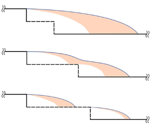
Streamlines of mean velocity and the out-of-plane vorticity component ( $\omega _z$) at all forcing frequencies, for step separations of $d=2h$, $d=4h$, and $d=6h$, are plotted in figure 3. Across the configurations shown, reattachment of the mean flow can occur on both steps, or only downstream of the second step, and varies significantly in streamwise position. To describe this variation, several measures of mean reattachment are presented. These measures include: the furthest downstream mean reattachment length in relation to the first step location, termed the total reattachment length ( $X_{r{,total}}$); the mean reattachment length on the first step in relation to the first step location ( $X_{r{,1}}$), which is only defined when reattachment on the first step occurs; the mean reattachment length on the second step in relation to the second step location ( $X_{r{,2}}$), which is only defined when reattachment on the first step occurs; and the combined length of detached flow ( $X_{r{,detached}}$). The combined length of detached flow is equivalent to $X_{r{total}}$ when no mean reattachment occurs on the first step, and $X_{r{,1}} + X_{r{,2}}$ when mean reattachment does occur on the first step. These measures of reattachment length are depicted in figure 1.
Streamlines of mean velocity and colour contours of the out-of-plane component of vorticity ( $\omega _z$) for $d=2h$ (a–f); $d=4h$ (g–l); and $d=6h$ (m–r). Panels (a,g,m) are the uncontrolled response. In subsequent panels the imposed forcing frequency is $St_h=0.077$ (b,h,n); $St_h=0.149$ (c,i,o); $St_h=0.374$ (d,j,p); $St_h=0.752$ (e,k,q); and $St_h=1.499$ (f,l,r). The $\blacktriangle$ (orange) markers indicate the mean reattachment location on the first (if applicable) and second steps.

The step separation of  $d=2h$ (figure 3a–f) provides a good representation of the drastic changes to the total reattachment length that occur for shorter step separations. With imposed forcing at $St_h=0.077$ and $St_h=0.149$, the mean flow field is somewhat akin to the UC response observed for the larger step separations of $3h\le d\le 4h$ (McQueen et al. Reference McQueen, Burton, Sheridan and Thompson2022b) – with a small counter-rotating flow structure just above the second-step base. This highlights how the position of the second step, in relation to the recirculation zone, influences the mean flow field. For the UC response, the total reattachment length was 2.3 and 3.4 times the streamwise step separation, for $d=3h$ and $d=4h$, respectively. Similar values were observed for $d=2h$ with imposed low-frequency forcing – with total reattachment lengths of 2.7 and 3.0 times the streamwise step separation with forcing at $St_h=0.077$ and $St_h=0.149$, respectively.
For  $d=4h$ (figure 3g–l), imposed forcing over $0.077\leq St_h\leq 0.752$ caused the flow to reattach on the first step. Over this forcing frequency range, the mean out-of-plane vorticity component is significantly stronger near reattachment on the first step, compared with near reattachment on the second step. When the flow reattaches on the first step, with forcing at $0.077\leq St_h\leq 0.149$ and, to a lesser extent for forcing at $St_h=0.374$, a region of strong vorticity is visible, extending downstream from the top corner of the second step.
The results for  $d=6h$ (figure 3m–r) provide a good representation of the effect of forcing for large step separations, where the flow reattaches on the first step regardless of forcing frequency. For forcing at $St_h\leq 0.374$, increased vorticity in the second recirculation zone is evident compared with the UC response. Low-frequency forcing shortens the first-step mean reattachment length and causes a reduction in the downwash at the second step. In figure 3(n–p), the mean streamlines approaching the second step are more aligned with the first-step floor than for the UC response (figure 3m).
3.1.2. Reattachment length
The effect of forcing on the total reattachment length ( $X_{r{,total}}$), the mean reattachment length on the first ( $X_{r{,1}}$) and second ( $X_{r{,2}}$) steps, as well as the combined length of detached flow ( $X_{r{,detached}}$) is shown in figure 4. In addition to the mean reattachment lengths, the difference between the UC response ( $X_{r,{UC}}$) and the result with imposed forcing ( $X_r$), calculated as ${\rm \Delta} X_{r}=(X_r-X_{r,{UC}})/X_{r,{UC}}$, is shown. The regions of white in figure 4(c,e) indicate configurations for which the mean flow does not reattach on the first step. In figure 4(d,f), comparison can only be made for $d\geq 5h$, where the mean flow reattaches on the first step for the uncontrolled response.
Colour maps of the total reattachment length (a,b), reattachment length on the first (c,d) and second (e,f) steps, and the total length of detached flow (g,h). Panels (b,d,f,h) show the variation from the UC response.

For the UC response, as reported by McQueen et al. (Reference McQueen, Burton, Sheridan and Thompson2022b), the total reattachment length reaches a minimum of  $X_{r{,total}}=8.58h$ for $d=5h$, and increases monotonically thereafter with increasing step separation. For $d\geq 5h$, there is a slight increase in first-step mean reattachment length with increasing step separation – from $X_{r{,1}}=4.62$ to $X_{r{,1}}=4.80$ over $d=5h$ to $d=8h$. Lastly, the mean reattachment length of the second recirculation zone is approximately $1h$ shorter than for the first over $d=5h$ to $d=8h$.
With imposed control, for small step separations ( $1h\le d\le 2h$), the change in total reattachment length resembles that typically observed for a BFS with equivalent forcing. Significant reduction in the total reattachment length occurs for the lowest and second-lowest forcing frequencies (figure 4b). Non-dimensionalised using the combined step height, the lowest forcing frequency is close to the step-mode instability for the BFS (identified as $St_H\approx 0.185$ by Hasan (Reference Hasan1992)). The second-lowest forcing frequency is close to the shear-layer instability for the BFS (identified as $St_\theta \approx 0.012$ by Hasan (Reference Hasan1992) and $St_\theta \approx 0.015$ by McQueen et al. (Reference McQueen, Burton, Sheridan and Thompson2022b) for this experimental set-up, which corresponds to $St_H\approx 0.3$ and $St_h\approx 0.15$).
The maximum variation (both reduction and increase) in the various measures of mean reattachment length with imposed forcing is shown in figure 5. The minimum total reattachment length,  $X_{r{,total}}=5.34h$, occurred for $d=2h$ with forcing at $St_h=0.077$ – a reduction of 48 % from the UC response. For all other step separations, including where the flow reattaches on the first step, the minimum in $X_{r{,1}}$, $X_{r{2}}$ and $X_{r{,total}}$ occurred for forcing at $St_h=0.149$ (figure 5a). The minimum at $d=2h$ is a result of a strong interaction between the large-scale structures generated by the imposed forcing and the second step. This is discussed further in § 3.2.3. There was comparatively little observed increase in the reattachment length for small step separations (figure 5b).
Maximum reduction (a) and increase (b) in  $X_{r{,1}}$ ( $\square$, black), $X_{r{,2}}$ ( $\triangle$, black), $X_{r{,total}}$ ( $\circ$, black), and $X_{r{,detached}}$ ( $\diamond$, black). The marker colour indicates the forcing frequency at which the maximum variation was observed: orange ( $St_h=0.077$), blue ( $St_h=0.149$), green ( $St_h=0.752$) and purple ( $St_h=1.499$).

For step separations of  $3h\le d\le 4h$, a reduction in the total reattachment length occurs over a broader range of forcing frequencies (figure 4a,b). There was no appreciable increase in reattachment length over $3h\le d\le 4h$ for any forcing frequency (figure 5b). Imposed forcing over $0.077\leq St_h\leq 0.374$ for $d=3h$, and $0.077\leq St_h\leq 0.752$ for $d=4h$, caused the flow to reattach on the first step (figure 4c). This did not happen until $d=5h$ for the UC response (McQueen et al. Reference McQueen, Burton, Sheridan and Thompson2022b).
For large step separations ( $d\geq 5h$), the typical BFS response is observed for the first recirculation zone. However, the first recirculation zone reattachment length is reduced for a broader range of forcing frequencies (figure 4d). Once mean reattachment on the first step occurs for the UC response ( $d\geq 5h$), there is still appreciable variation in the second-step mean reattachment length under imposed forcing (figure 4e,f). For $d\geq 6h$, an up to 6 % decrease in the second-step mean reattachment length (figure 5a) and an up to 9 % increase (figure 5b) occurred.
For the UC response, the combined length of detached flow was at a minimum for  $d=6h$, where the mean flow reattached on the first step and the downwash over the second step caused a large mean reattachment length reduction. With imposed forcing, the minimum combined length of detached flow occurred at $d=2h$, although comparable reductions were achieved for $2h\le d\le 4h$ with low-frequency forcing (figure 4g,h).
3.1.3. Surface pressure
McQueen et al. (Reference McQueen, Burton, Sheridan and Thompson2022b) detailed the variation in mean base pressure for the DBFS flow, up to a step separation of  $d=8h$. For $d\le 2h$, minimal variation between each step mean base pressure was observed. Thereafter, the mean base pressure on each step changed quickly. For $d\ge 3h$, the second-step mean base pressure is primarily a function of the second-step position in relation to the pressure rise that occurs in the recirculation zone downstream of the first step. The peak second-step mean base pressure occurred for $d=6h$. Conversely, the first-step mean base pressure reduced to a minimum at $d=5h$, a result of interaction between the first and second recirculation zones.
Figure 6 shows the influence of forcing on the mean base pressure averaged over the height of the first-step ( $\overline {C_{p,1}}$), second-step ( $\overline {C_{p,2}}$) and the height of the two steps combined ( $\overline {C_p,c}$), along with comparisons with the results for the UC response ( $\overline {C_{p,1,{UC}}}$, $\overline {C_{p,2,{UC}}}$, $\overline {C_{p,c,{UC}}}$). As for mean reattachment length, significant variation in mean base pressure occurs with imposed forcing. For the BFS, McQueen et al. (Reference McQueen, Burton, Sheridan and Thompson2022a) noted that, with imposed forcing, the trend in mean base pressure variation followed that of mean reattachment length. However, for the DBFS flow, a more complex relationship exists.
Colour maps of mean base pressure on the two steps combined (a,b), the first step (c,d) and the second step (e,f).

For  $1h\le d\le 2h$, the mean combined base pressure variation (figure 6a,b) follows a similar trend to the BFS, as is the case for total reattachment length. The maximum mean combined base pressure reduction across the investigated parameter space ( $\overline {C_p,c}-\overline {C_{p,c,{UC}}}=-0.051$) occurs for $d=1h$, with forcing at $St_h=0.149$. By $d=3h$, however, the trend in mean base pressure deviates from that of mean reattachment length. At $3h\le d\le 4h$, for all but the highest forcing frequency, a reduction in mean base pressure on the first step, and an increase on the second step, occurs. The maximum variation from the UC response on both steps occurs for forcing at $St_h=0.149$ over this step separation range. In contrast to the situation for mean reattachment length, where a reduction was observed at all forcing frequencies, there is an increase in the mean combined base pressure for $3h\le d\le 4h$. This variation may be primarily attributed to the shift in mean reattachment location in relation to the second step and associated changes in surface pressure discussed below. By $d=5h$, reattachment occurred on both steps for all forcing frequencies. A return towards resemblance of the BFS profile is seen for the mean combined base pressure, with a reduction for low forcing frequencies and an increase for high forcing frequencies.
Figure 7 shows the mean floor pressure with imposed forcing, along with results for the UC response. As for the BFS, there are large differences in mean surface pressure across the forcing frequency parameter space. This is particularly the case for low-frequency forcing; the most prominent differences being the upstream shift of the pressure rise – commensurate with the upstream shift of the mean reattachment location – and the reduction in pressure near the base of the first step. For low-frequency forcing, by  $d=3h$ (figure 7c), mean pressure on the first-step floor rises above that for the UC response. This is due to a significant component of the pressure rise through the reattachment region occurring upstream of the second step. By $d=5h$ (figure 7e), for all forcing frequencies and the UC response, the flow reattaches on the first step and the pressure rise through reattachment reaches, or almost reaches, a local maximum upstream of the second step. There is significantly less variation in the mean surface pressure downstream of the second step for $d\geq 5h$.
Mean pressure on the first-step and second-step floors for step separations of  $d=1h$ (a); $d=2h$ (b); $d=3h$ (c); $d=4h$ (d); $d=5h$ (e); $d=6h$ (f); $d=7h$ (g); and $d=8h$ (h). The dashed black lines show the second-step base location.

Roshko & Lau (Reference Roshko and Lau1965) demonstrated that the pressure rise through reattachment for a BFS (as well as for several other geometries) could be collapsed by normalising the pressure by the minimum pressure,  $C_p^{*} = (C_p-C_{p,min})/(1-C_{p,min})$, and the streamwise distance by the reattachment length. For the BFS at high Reynolds numbers, Adams & Johnston (Reference Adams and Johnston1988) were able to show that this normalisation holds well for small boundary-layer heights. However, with $\delta /H\gtrsim 0.4$, a steady decrease in the peak pressure downstream of reattachment occurs. For the uncontrolled response of the DBFS flow, McQueen et al. (Reference McQueen, Burton, Sheridan and Thompson2022b) observed that, when the flow reattaches on the first step, the pressure rise through the first reattachment zone is insensitive to the step separation; however, the total pressure rise is slightly less than for the BFS. This is likely due to the change in the boundary-layer height to step height ratio, with a change in relevant scaling from the combined to single-step height for large step separations. For the second recirculation zone, a significantly lower pressure rise through reattachment occurred – although as the step separation was increased, the pressure rise trends towards that observed for the first recirculation zone.
With imposed periodic forcing, the normalised pressure distributions are affected for all step separations investigated. Figure 8 shows the effect of forcing for a step separation of  $d=8h$, which is representative of step separations where the flow reattaches on both steps. For the UC response, good agreement with the BFS response is seen through the first recirculation zone up to reattachment (figure 8a). Thereafter, the two responses deviate with a lower peak pressure rise for the DBFS. For all imposed forcing frequencies, there is more deviation from the BFS profile. For low-frequency forcing ( $0.077\leq St_h\leq 0.149$), the pressure rise occurs farther upstream in the recirculation zone, with a peak value greater than the UC response (figure 8a). Conversely, for higher forcing frequencies, a lower pressure rise through reattachment occurs. Nash (Reference Nash1963) discussed how the pressure rise through reattachment is an important mechanism that maintains a balance between entrainment in the shear layer and flow reversal upstream from near reattachment. Berk et al. (Reference Berk, Medjnoun and Ganapathisubramani2017) demonstrated that imposed periodic forcing around the shear-layer instability increases shear-layer entrainment, and that higher frequency forcing ( $St_H=1.98$) decreases entrainment. The results in figure 8(a) are evidence of this balance that occurs in the recirculation zone. The low-frequency forcing increases entrainment in the shear layer, and consequently the pressure rise through reattachment is increased – and vice versa for high-frequency forcing. For a BFS, the pressure rise downstream of the step base may not be of practical importance. However, for the DBFS, controlling the location and magnitude of the pressure rise through reattachment on the first step can have a large influence on the second-step mean base pressure. This effect on the second step can be at least as significant as controlling the first-step base pressure, in terms of changes to the combined base pressure, which is likely of practical interest.
Mean pressure profile on the first-step (a) and second-step (b) floors for  $d=8h$, in the reduced coordinates of Roshko & Lau (Reference Roshko and Lau1965). The grey dashed line shows the results for the BFS.

The pressure recovery through reattachment of the second recirculation zone is strongly influenced by the flow conditions upstream of the second step. As can be seen in figure 8(b), there is little variation in the normalised pressure near the second-step base, with significant variation only occurring downstream of  $(x-X_{r,2})/X_{r,2}\approx -0.25$. This is similar to the variation observed by Adams & Johnston (Reference Adams and Johnston1988) when altering the upstream boundary layer, which resulted in a decrease in the maximum mean pressure with increasing boundary-layer height. Figure 9 shows the mean streamwise and wall-normal velocity profiles above the second-step base for $d=8h$. While, for all forcing frequencies, the mean profiles still vary significantly from that of the BFS, for $0.077\leq St_h\leq 0.149$ there is higher mean streamwise velocity near the first-step floor and less downwash above the second step. As is discussed in § 3.2.3, for $d=8h$, forcing at $0.077\leq St_h\leq 0.149$ results in the generation of large-scale flow structures that extend down to the first-step floor. These structures draw higher momentum flow down near the first-step floor, resulting in the higher velocity observed below $y/h\approx -0.25$ in figure 9(a) for $0.077\leq St_h\leq 0.149$. The higher pressure rise observed through reattachment of the second recirculation zone with low-frequency forcing (figure 8b) is a result of two influences. Firstly, the increase in streamwise velocity above the step at flow separation is expected to alter the development of the shear layer in a similar manner to a reduction in the boundary-layer height (Adams & Johnston Reference Adams and Johnston1988). Secondly, as will be discussed in § 3.2, perturbations at the forcing frequency persist sufficiently far downstream to influence the development of the second recirculation zone, contributing to the increased pressure rise in the same manner as for the first recirculation zone.
Streamwise (a) and wall-normal (b) velocity profiles above the second-step base ( $x/h=8$) for $d=8h$. The dashed orange line shows the profile for the BFS configuration without imposed control. Markers are shown for every 12th velocity vector.

3.2. Dynamic flow characteristics
3.2.1. Reynolds stresses
For a BFS, Ma et al. (Reference Ma, Geisler, Agocs and Schröder2015) decomposed Reynolds shear stress into coherent and incoherent components. They demonstrated that, with imposed periodic forcing close to the shear-layer instability, there are two main effects on the turbulent fluctuations in the flow. The coherent component contributes to increased Reynolds shear stress in a localised area in the separated shear layer, due to the roll-up of spanwise vortices. The incoherent component contributes to an increase in Reynolds shear stress across the entire shear layer. Likewise, here with imposed forcing at  $St_h=0.149$ (close to the shear-layer instability), there is a significant increase in the Reynolds shear stress for all step separations (figure 10f–j). For $d=1h$ and $d=2h$, there is a region of strong Reynolds shear stress in the shear layer just upstream of reattachment, as for the BFS. In addition, there is increased Reynolds shear stress above the second-step base, where interaction between the reverse flow up over the second step and the shear layer occurs. By $d=3h$, the peak Reynolds shear stress occurs upstream of the second step. By $d=5h$, the Reynolds shear stress distribution resembles that of two distinct BFS flows, albeit with higher levels of Reynolds shear stress in the first recirculation zone. A return towards a distinct region of high Reynolds shear stress, downstream of each step, occurs at larger step separations for the UC response, compared with that of imposed low-frequency forcing (figure 10a–e). This is a result of the greatly shortened reattachment length where there is imposed low-frequency forcing. With high-frequency forcing ( $St_h=1.499$) (figure 10k–o), the Reynolds shear stress distribution for all step separations closely resembles that of the UC response, aside from a localised region of increased Reynolds shear stress in the shear layer, just downstream of flow separation. This location is where Ma et al. (Reference Ma, Geisler, Agocs and Schröder2015) identified an increase in the coherent component of Reynolds shear stress due to the roll-up of vortices.
Normalised Reynolds shear stress ( $\overline {u^{\prime }v^{\prime }}/U_{ref}^{2}$) for $d=1h$ (a,f,k); $d=2h$ (b,g,l); $d=3h$ (c,h,m); $d=5h$ (d,i,n); and $d=8h$ (e,j,o). Panels (a–e) show the UC response, (f–j) forcing at $St_h=0.149$ and (k–o) forcing at $St_h=1.499$. The $\blacktriangle$ (orange) markers indicate the mean reattachment location on the first (if applicable) and second steps. The $\bullet$ (orange) markers indicate the locations of the PSD estimates in figure 14.

3.2.2. Surface pressure
For a BFS with imposed forcing, Benard et al. (Reference Benard, Sujar-Garrido, Bonnet and Moreau2016) found a maximum reduction in mean reattachment length when forcing at the shear-layer instability. However, they found that the maximum surface-pressure fluctuations ( $\sigma _{C_p}$) occur when forcing at the subharmonic of the shear layer instability ( $St_H=0.125$), which is somewhat close to the step-mode instability ( $St_H\approx 0.185$). The increase in surface pressure fluctuations was a result of the large-scale vortices (on the scale of the step height) that form due to a vortex pairing process in the shear layer. As evident in figure 11, for the two lowest forcing frequencies ( $St_h=0.077$ and $St_h=0.149$), a significant increase in the standard deviation of surface pressure occurs for all step separations. Given that the step-mode instability has been shown to scale with step height at $St_H\approx 0.185$ (Hasan Reference Hasan1992), here the effect of forcing is likely different for small and large step separations, with a change in the relevant characteristic length from the combined- to single-step height. Scaling with the combined step height, the lowest forcing frequency, $St_H=0.153$ ( $St_h=0.077$), is closest to the step-mode instability. Scaling with the single-step height, the second-lowest forcing frequency is closest to the step-mode instability at $St_h=0.149$.
Standard deviation of pressure on the first-step and second-step floors for step separations of  $d=1h$ (a); $d=2h$ (b); $d=3h$ (c); $d=4h$ (d); $d=5h$ (e); $d=6h$ (f); $d=7h$ (g); and $d=8h$ (h). The solid black lines show the results for the BFS. The dashed black lines show the second-step base location.

For a step separation of  $d=1h$ (figure 11a), the standard deviation of pressure on the two step floors resembles that seen for a BFS, with peak fluctuations occurring near reattachment. Forcing at $St_h=0.077$ results in peak fluctuations of $\sigma _{C_p}=0.128$, three times that of the $\sigma _{C_p}=0.041$ observed for the UC response. By $d=3h$ (figure 11c), the peak fluctuations occur on the first step for the two lowest forcing frequencies. There is also less difference between the peak magnitude of fluctuations for the two lowest forcing frequencies. In general, the development of the standard deviation of surface pressure on the first-step floor for low-frequency forcing is not strongly influenced by the location of the second step (figure 12). As for the BFS with imposed forcing, it is expected that the development of vortex structures in the shear layer, and their interaction with the step floor as they progress downstream, are the primary contributors to surface-pressure fluctuations. With imposed low-frequency forcing for large step separations ( $d\ge 6h$), the standard deviation of surface pressure has significantly reduced by the second step (figure 11f–h). However, it builds again in the second recirculation zone; evidence that the vortex structures generated in the first recirculation zone persist sufficiently far downstream to influence the development of the second recirculation zone. With higher frequency forcing the results vary less from the UC response. The most noticeable difference is an increase in surface-pressure fluctuations close to the first-step base.
Standard deviation of pressure on the first-step floor with imposed forcing at  $St_h=0.077$ (a) and $St_h=0.149$ (b).

From figure 11 it is evident that the imposed forcing has a strong influence on the surface pressure for the DBFS. To reveal the dynamics of this influence, space–time plots of surface pressure for the UC response and forcing at  $St_h=0.077$ and $St_h=0.149$, for which a large standard deviation of surface pressure was observed, are shown in figure 13. For the BFS, Lee & Sung (Reference Lee and Sung2002) plotted space–time distributions of surface pressure over $2\le x/H\leq 9.75$. They noted the presence of instantaneous low-pressure peaks, which have been shown to indicate the passing of large-scale vortices for the BFS (Cherry, Hillier & Latour Reference Cherry, Hillier and Latour1984). They also observed high-pressure peaks, associated with the ‘downward inrush of free stream between vortices’. The inclined pattern in the space–time distributions was noted as evidence of the positive convection velocity of vortices.
Space–time contour plots of instantaneous wall pressure for step separations of  $d=1h$ (a); $d=2h$ (b); $d=3h$ (c); and $d=8h$ (d). Panel (i) shows the UC response, (ii) imposed forcing at $St_h=0.077$ and (iii) $St_h=0.149$. The black line depicts the position of the second-step base.

For  $d=1h$, faint traces of pressure fluctuations are visible downstream of $x/h\approx 5$ for the UC response (figure 13ai). This location is close to mean reattachment, where vortex structures in the shear layer approach the step floor. The signatures of the passage of vortex structures remain visible up to the furthest downstream distance at which measurements were acquired. Similar trends for the UC response can be observed for step separations of $d=2h$ (figure 13bi) and $d=3h$ (figure 13ci); however, by $d=8h$ (figure 13di), the formation of two distinct flow separation zones is evident. A low pressure zone is visible, with an inclined pattern of peaks in pressure extending downstream of each step. In certain instances, when a large pressure fluctuation occurs over the first step, the signature in the space–time plot remains coherent downstream of the second step – suggesting the persistence of a large flow structure far downstream – but, in general, there is no clear link between fluctuations on each step. For $d=8h$, the inclined streaks of pressure fluctuations are spaced closer together, indicating an increase in the frequency of fluctuations when the flow reattaches on both steps.
With imposed forcing at  $St_h=0.077$, for short step separations ( $d\leq 3h$) (figure 13aii, bii,cii), strong pressure fluctuations are visible extending from the first-step base, downstream to the furthest measurement location. There is a clear alignment of the fluctuations upstream and downstream of the second step. Evidence of more complex behaviour is also apparent. While there are clear, periodic fluctuations on the first-step floor at the forcing frequency, downstream of the second step alternate inclined streaks either persist far downstream or dissipate close to the second-step base. This suggests that a vortex-merging process occurs downstream of the second step, reducing the frequency of the fluctuations to the subharmonic of the imposed forcing frequency. This behaviour is most apparent for $d=2h$, although also occurs intermittently for $d=3h$, and to a lesser extent for $d=1h$. For $d=8h$, the inclined patterns of pressure fluctuations originating near the first-step base persist far downstream of the second step.
For forcing at  $St_h=0.149$, as expected from figure 11, the instantaneous pressure fluctuations are not as strong as for the lowest forcing frequency. For $d=2h$ (figure 13biii), there is some evidence of a reduction in the frequency of fluctuations to the subharmonic downstream of the second step. However, for forcing at $St_h=0.149$, this is less clear than for forcing at $St_h=0.077$. By $d=8h$ (figure 13diii), there is only a weak indication of flow structures from the first recirculation zone persisting sufficiently far downstream to influence the second step surface pressure.
3.2.3. Power spectra
With imposed low-frequency forcing, there are large increases in Reynolds shear stress across the spatial domain, and also strong surface-pressure fluctuations. To better understand the frequency content of the fluctuations in the flow, power spectral density (PSD) estimates of streamwise velocity throughout the flow field are shown in figure 14. The locations of the PSD estimates are shown in figure 10(b,c,e). These locations were chosen to show the variation in the PSD estimates from near the first step to far downstream. The PSD estimates were calculated using Welch's method with a Hanning window, using sample lengths of 1000 data points and 50 % overlap (Welch Reference Welch1967). Figure 14 shows PSD estimates for the three lowest forcing frequencies for step separations of  $d=2h$ and $d=3h$, where large surface pressure fluctuations were observed, and where it appeared a vortex-merging process occurred downstream of the second step. Results for $d=8h$ are also shown, where mean reattachment occurs on both steps, and the single-step height is a more relevant characteristic length. With imposed forcing at $St_h=0.077$, for $d=2h$ and $d=3h$, a sharp peak in the spectra at the forcing frequency is dominant, to a distance of approximately $2h$ downstream of the second-step base (figure 14a,d). Thereafter, the subharmonic of the forcing frequency is more prominent. Close to the first-step base, smaller peaks at higher harmonics of the forcing frequency can also be observed. For $d=8h$, the forcing frequency remains dominant over the entire spatial domain (figure 14g).
The PSD estimates of the streamwise velocity for step separations of  $d=2h$ (a–c), $d=3h$ (d–f) and $d=8h$ (g–i) at the locations indicated by the $\circ$ (orange) markers in figure 10. Imposed forcing at $St_h=0.077$ (a,d,g), $St_h=0.149$ (b,e,h) and $St_h=0.374$ (c,f,i). Each PSD estimate is separated by two decades. The blue estimates are located at, or upstream of, the second-step base. The black estimates are located downstream of the second-step base. The orange solid lines indicate the imposed forcing frequency, and the dashed lines the first lower and higher harmonics.

With forcing at  $St_h=0.149$, for all step separations there are distinct spectral peaks at the forcing frequency in the shear layer near the first-step base (figure 14b,e,h). There are also smaller peaks at higher harmonics. As for the lowest forcing frequency, $St_h=0.149$ remains dominant downstream of the second-step base, for a distance of approximately $2h$. For $d\ge 3h$ (figure 14e), the power of the subharmonic increases moving downstream, becoming the dominant frequency prior to the second step. With forcing at $St_h=0.374$, for all step separations there is a sharp spectral peak at the forcing frequency close to the first-step base, although, this quickly diminishes moving downstream (figure 14c,f,i).
3.2.4. Phase-averaged results
To better understand the development of the large-scale flow structures that occurs over an actuation cycle with low-frequency forcing ( $0.077\le St_h\le 0.149$), phase-averaging of the PIV and surface pressure data was conducted. Using the pressure tap on the first-step base 6 mm (0.03 $y/H$) below the actuation slot, the PIV snapshots and base-pressure measurements were divided into 24 phases. Figure 15 shows phase-averaged streamlines and colour contours of the $\varGamma _2$ criterion – which indicates regions where rotation dominates strain in the flow (Graftieaux, Michard & Grosjean Reference Graftieaux, Michard and Grosjean2001) – for four equally spaced phases with imposed forcing at $St_h=0.077$. The phase-averaged base pressure on each step and phase-averaged total reattachment length for the 24 phases are also shown.
Phase-averaged streamlines and colour contours of  $\varGamma _2$ for step separations of $d=1h$ (a), $d=2h$ (b), $d=3h$ (c) and $d=8h$ (d), with imposed forcing at $St_h=0.077$. The interrogation domain is $9\times 9$ vectors $^{2}$. Each contour plot is separated by a quarter cycle. Blue contours show clockwise rotation, red contours show anticlockwise rotation. The $\blacktriangle$ (orange) markers indicate phase averaged reattachment locations. The phase-averaged base pressure on the first (solid blue line) and second (dashed blue line) steps, phase averaged total reattachment length ( $\bullet$, orange) and phase averaged reattachment on the first step ( $\blacksquare$, orange) are also shown below the contour plots.

Figure 15 shows the growth of large-scale flow structures, primarily downstream of the second-step base. These flow structures extend down to the step floor, causing the large periodic base-pressure fluctuations observed. For the first phase pictured (figure 15ai), there is no blowing or suction from the slot. A strong clockwise-rotating (blue) structure, on the scale of the combined-step height, can be observed close to the second-step base. This structure causes strong upwash over the second-step base, resulting in the formation of a smaller, anticlockwise-rotating (red) structure above the first-step floor. At the peak of the blowing phase (figure 15aii), a new clockwise rotating structure begins to form just downstream of separation from the first step. This structure is not yet visible in the streamlines plotted. In this second phase, the clockwise-rotating structure behind the second-step base has convected downstream, resulting in a pressure rise on the second-step base as the low-pressure vortex core moves away. As this flow structure convects downstream, the upwash that feeds the anticlockwise-rotating structure above the first-step floor is reduced, and that structure dissipates. At a phase of  ${\rm \pi}$ (figure 15aiii), after the blowing and before the suction phase, the flow is angled downwards at flow separation from the first step and the clockwise-rotating structure generated during the blowing phase is visible above the first-step floor. During the peak suction phase (figure 15aiv), the new clockwise-rotating structure moves downstream of the second-step base, and appreciable flow reversal back over the second-step base is visible once more. There is slightly less than a 90 $^{\circ }$ phase delay between base-pressure fluctuations on the first and second step over the actuation cycle.
By  $d=2h$, there is no longer a large anticlockwise-rotating structure generated over the length of the first-step floor between the suction and blowing phases. Rather, a clockwise-rotating region of flow is present near the first-step base for all 24 phases. In figure 15(bi), the upwash at the second-step base flows up over the step corner and back upstream, resulting in a single large flow structure shaped around the second-step top corner. At the peak blowing phase (figure 15bii), this structure has split off from flow above the first step, and as for a step separation of $d=1h$, a new clockwise-rotating structure begins to form. By the peak suction phase (figure 15biv), the newly generated structure grows and convects downstream, connecting the regions of clockwise rotating flow upstream and downstream of the second-step base once more.
For  $d=3h$, similar behaviour occurs as for $d=2h$, albeit with a greater delay between the effects of the large-scale flow structures on the first- and second-step bases. For $1h\le d\le 3h$, essentially the same observations downstream of the second-step can be made, however, there is an increase in the phase delay of approximately 90 $^{\circ }$ for every $1h$ increase in step separation. For example, compare the flow structure near the second-step base and base pressure on each step (indicated by the blue lines in figure 15) for figure 15(ai), figures 15(bii) and 15(ciii).
The space–time plots of surface pressure and PSD estimates of streamwise velocity indicate that a vortex-merging process likely occurs downstream of the second-step base, for short step separations when forcing at  $St_h=0.077$. No direct evidence of this could be discerned from the phase-averaged data. However, downstream of the second step, an acceleration of the large-scale structures is evident (figure 15a–c). For a BFS, Benard et al. (Reference Benard, Sujar-Garrido, Bonnet and Moreau2016) used a similar phase-averaging technique, with imposed forcing at the shear-layer instability and its subharmonic. When forcing at the subharmonic of the shear-layer instability, they noted that a vortex-pairing process occurs, which results in a temporary reduction in the convection velocity of large-scale flow structures, followed by a subsequent acceleration. Potentially, for the results shown here, the vortex-merging process is masked both by the presence of the recirculating flow downstream of the second step and the analysis techniques used.
Benard et al. (Reference Benard, Sujar-Garrido, Bonnet and Moreau2016) also observed similar trends in the phase-averaged reattachment length to those observed here. When forcing at the subharmonic of the shear-layer instability, the reattachment length was observed to increase monotonically by approximately  $1H$ over the majority of an actuation cycle, before rapidly reducing in a sawtooth-like pattern. They discussed how the reattachment location is drawn downstream with the convection of a large-scale flow structure, until that structure detaches from the wall and the reattachment location moves back upstream (Dejoan & Leschziner Reference Dejoan and Leschziner2004; Benard et al. Reference Benard, Sujar-Garrido, Bonnet and Moreau2016). This phenomenon is evident in the phase-averaged total reattachment length shown in figure 15(a–c), which fluctuates by approximately $2h$ to $2.5h$ ( $1H$ to $1.5H$). This pattern is also observed in the phase-averaged reattachment on the first step in figure 15(d) which fluctuates by approximately $1.8h$.
Phase-averaging of the PIV, with imposed forcing at  $St_h=0.149$ is shown in figure 16. Note that for $d=3h$ (figure 16c), the phase-averaged total reattachment length was ill-defined over phase angles of $3{\rm \pi} /2$ to $2{\rm \pi}$ and as such is not shown. For $d\le 3h$, initial development of vortex structures and interaction with the second-step base are similar to those observed for the lowest forcing frequency (shown in figure 15). Although, with the doubling of the forcing frequency, there is also a doubling of the phase delay between pressure fluctuations on each step base, to an increase of approximately 180 $^{\circ }$ for a $1h$ increase in step separation. For these short step separations, there is no obvious acceleration of the large-scale structures downstream of the second step, and there is significantly less reattachment length variation over an actuation cycle than for forcing at $St_h=0.077$. For $d\le 3h$, the reattachment length varies by approximately $0.5h$ ( $0.25H$) and resembles a triangular waveform. This behaviour was also observed by Benard et al. (Reference Benard, Sujar-Garrido, Bonnet and Moreau2016) when forcing at the shear-layer instability. However, by $d=8h$ (figure 16d), the behaviour seen for forcing at the lowest forcing frequency returns. The reattachment length varies by approximately $1h$ ( $0.5H$) in a profile that more closely resembles the sawtooth pattern seen in figure 15. Some acceleration of the large-scale flow structures above the first-step floor is also evident.
Phase-averaged streamlines and colour contours of  $\varGamma _2$ for step separations of $d=1h$ (a), $d=2h$ (b), $d=3h$ (c) and $d=8h$ (d), with imposed forcing at $St_h=0.149$. See figure 15 for further details.

4. Flow regimes
For the UC response of the DBFS flow, McQueen et al. (Reference McQueen, Burton, Sheridan and Thompson2022b) categorised the flow into three regimes based on the step separation in the streamwise direction. The addition of imposed forcing results in significantly more variation in the key flow characteristics. Here, the flow over a DBFS with imposed forcing has been characterised into three regimes based on step separation, with the additional characterisation of low- and high-frequency forcing effects.
4.1. Regime A: BFS-like behaviour
For short step separations ( $d\lesssim 3h$), the effect of imposed periodic forcing on the DBFS flow is similar to that for the BFS. Forcing at $St_h=0.149$ ( $St_H=0.297$), which is close to the shear-layer instability for the BFS, produces the maximum reduction in both the total reattachment length and combined base pressure (see figures 4 and 6). The lowest forcing frequency, $St_h=0.077$ ( $St_H=0.153$), is close to the step-mode instability for the BFS and generates large-scale flow structures that extend down to the step floor, as depicted in figure 17(a). This results in the maximum floor and base pressure fluctuations on both steps, with a maximum increase in floor pressure fluctuations of approximately 360 % over the UC response (see figure 11). The downstream convection of the large-scale structures generated causes periodic base-pressure fluctuations on each step base. An increase in the phase delay between the instantaneous base pressure on each step base, of approximately 90 $^{\circ }$, occurs for a $1h$ increase in step separation. As for the BFS, low-frequency forcing results in increased Reynolds shear stress throughout the flow field (figure 10). For low forcing frequencies, a consequence of the reduced reattachment length is a stronger interaction between the separated shear layer and the second-step top corner. Contrarily, at the highest forcing frequency ( $St_h=1.499$), there is a slight increase in the total reattachment length and base pressure, due to a decrease in flow entrainment in the shear layer (Berk et al. Reference Berk, Medjnoun and Ganapathisubramani2017) (figure 17b). The high-frequency forcing also causes an increase in the floor and base-pressure fluctuations over the first part of the recirculation zone ( $x/h\lesssim 5$), similar to that seen to occur for the BFS (McQueen et al. Reference McQueen, Burton, Sheridan and Thompson2022a).
Diagrams depicting some key features of the identified flow regimes. (a,c,e) Low-frequency forcing response. (b,d,f) High-frequency forcing response. The solid blue line shows the approximate uncontrolled separating streamline. The shaded orange regions show the approximate range of controlled separating streamlines.

4.2. Regime B: controlled reattachment and large base pressure variation
For step separations of  $2.5h\lesssim d\lesssim 4.5h$, there is no longer a resemblance to the BFS response. The total reattachment is reduced for all but the highest forcing frequency, for which there is only a slight increase in reattachment length ( $\approx 1\,\%$). For $d=3h$ and $d=4h$, with imposed forcing over $0.077\leq St_h\leq 0.374$ and $0.077\leq St_h\leq 0.752$, respectively, the flow reattached on the first step. This did not occur until $d=5h$ for the uncontrolled response. There was an increase in combined base pressure for all forcing frequencies. For low forcing frequencies, this increase occurs as the location of the second step coincides with the peak pressure rise downstream of the first recirculation zone (see figure 7), causing a large increase in second-step base pressure. When the forcing shortens the total reattachment length, or causes reattachment on the first step, there is a significant reduction in first-step base pressure (figure 17c). This has also been observed for the BFS. In this regime, peak Reynolds shear stress occurs above the first step for all but the highest forcing frequency. There are minimal changes to the mean flow field with high-frequency forcing (figure 17d).
4.3. Regime C: a shift in the dynamic characteristics
By  $d=5h$ the flow reattaches on the first step for the UC response and for all forcing frequencies. Considering the first recirculation zone, the flow once more behaves like that of a BFS, with peak reduction in both the first-step reattachment length and base pressure when forced at $St_h=0.149$ (see figures 4 and 6). Reynolds shear stress and surface-pressure fluctuation magnitudes are comparable with those of shorter step separations (see figures 10 and 11). However, there is an apparent shift in the dynamic behaviour of the flow. For the BFS, Benard et al. (Reference Benard, Sujar-Garrido, Bonnet and Moreau2016) identified different flow behaviours when forcing at the shear-layer instability and its subharmonic. These behaviours are reported in § 3.2, including: sawtooth versus triangular profiles of reattachment length variation; varying magnitudes of reattachment length fluctuation; and shifts in the dominant frequency observed in the wake. Importantly, the change in relevant characteristic length from the combined-step height to the single-step height, when moving from small to large step separations, altered the dynamic characteristics of the flow.
For low forcing frequencies, fluctuations at the forcing frequency persisted sufficiently far downstream to influence the development of the second recirculation zone. This is most evident in the growth of surface pressure fluctuations in the second recirculation zone (see figure 11). This influence causes a reduction in the second recirculation zone reattachment length, albeit only up to approximately 60 % of that observed for the first recirculation zone (figure 17e). This reduction in reattachment length occurred despite a reduction in the mean downwash over the second step, which, by itself, would likely cause an increase in reattachment length. The reduction in downwash is a result of the shorter first recirculation zone. With the shorter recirculation zone, there is a greater distance, between the first step reattachment location and the second step, for the flow to be redirected in the streamwise direction. The maximum increase in the reattachment length of the second recirculation zone of approximately 9 % was observed for  $d=6h$, with imposed forcing at $St_h=0.752$ (figure 17f). This increase results from a combination of two factors. A moderate reduction in the first step reattachment length, which reduces the downwash. This is accompanied by a more rapid decay of fluctuations at the forcing frequency than those seen at lower forcing frequencies, which minimises influence on the development of the second recirculation zone. Lower forcing frequencies more strongly influence the second recirculation zone, and higher forcing frequencies do not reduce the upstream reattachment length or associated downwash. In this third regime, there are no longer the large-scale variations in base pressure that were observed for $2.5h\lesssim d\lesssim 4.5h$.
5. Conclusion
Periodic forcing was imposed on the DBFS flow, with streamwise step separation varying over  $1h\le d\le 8h$. The imposed forcing significantly altered both the mean and dynamic characteristics of the flow over much of the step separation and forcing frequency parameter space. Key findings were distilled into three flow regimes based on the step separation and forcing frequency.
For a step separation of  $d\lesssim 2.5$, the flow largely behaved like that of a BFS with equivalent forcing. Forcing around the frequency of the shear-layer instability of the BFS resulted in a maximum reduction in both the mean reattachment length and combined base pressure. Forcing at lower frequencies resulted in a comparable reduction in the reattachment length, albeit with stronger floor- and base-pressure fluctuations. These resulted from the generation of large-scale flow structures that extended down to the step floor. When forcing close to the step-mode instability, the large base-pressure fluctuations on the second step were found to lag those on the first step by $\sim 90^{\circ }$ for $d=1h$. This delay increased by a further ${\sim} 90^{\circ }$ with a $1h$ increase in step separation, up to $d\approx 3h$. At the highest forcing frequency ( $St_h=1.499$), there was a slight increase in base pressure on both steps, but with little observable change to the mean flow field from the UC response.
Increasing the step separation further to  $2.5h\lesssim d\lesssim 4.5h$ produced the most significant differences from comparable BFS forcing. For the UC response, the flow only reattaches on the first step for $d\ge 5h$, but this could be reduced to $d=3h$ with forcing over $0.077\leq St_h\leq 0.374$, and $d=4h$ with forcing over $0.077\leq St_h\leq 0.752$. Concomitant with the reduced reattachment length, the pressure rise through the reattachment region moved upstream over these forcing frequency ranges, resulting in a large increase in the second-step base pressure. Consequently, the combined base pressure was increased for all forcing frequencies in this regime. For $d\ge 3h$, both the surface-pressure fluctuations and Reynolds shear stress peaked upstream of the second step.
For  $d\gtrsim 4.5h$, if the first step is considered in isolation, the flow behaves like that of a BFS, with a decrease in reattachment length and base pressure when forcing at $St_h\lesssim 0.752$. While a slight reduction in the second-step base pressure was observed for nearly all forcing conditions for $d\gtrsim 4.5h$, an increase in second-step reattachment length of up to approximately 9 % occurred (for $d=6h$ with forcing at $St_h=0.752$). It appears that the second-step reattachment length is a balance between a reduction in downwash over the second step, and downstream persistence of fluctuations at the forcing frequency. Lastly, there was a shift in the dynamic behaviour of the flow with imposed low-frequency forcing when moving from short to large step separations.
In this study we have demonstrated that imposed periodic forcing can significantly alter the global flow characteristics of the DBFS flow. This work shows, for the first time, the potential to control the flow over this fundamental geometry. Consequently, it also offers insight into how to implement performance improvements in applications such as the drag reduction of vehicles like pickup trucks. The combined base pressure on the two steps could be increased, an indication that vehicle drag could be reduced. However, the base pressure increase came at the cost of higher levels of surface pressure fluctuation, which may be detrimental in certain applications.
Funding
This research used equipment that was partially funded by the Australian Government through the Australian Research Council's Linkage Infrastructure, Equipment and Facilities program (project number LE170100203). T.M. acknowledges the financial support of an Australian Government Research Training Program Scholarship.
Declaration of interests
The authors report no conflict of interest.


 Open access