


1 Introduction
Since the creation of the first laser by Theodore Meiman in 1960[ Reference Maiman 1 ], pulse peak power has been constantly growing and has recently reached the multipetawatt level. Many laboratories in the world have a laser with a power of 1 PW or more[ Reference Danson, Bromage, Butcher, Chanteloup, Chowdhury, Galvanauskas, Gizzi, Haefner, Hein, Hillier, Hopps, Kato, Khazanov, Kodama, Korn, Li, Li, Limpert, Ma, Nam, Neely, Papadopoulos, Penman, Qian, Rocca, Shaykin, Siders, Spindloe, Szatmári, Trines, Zhu, Zhu and Zuegel 2 – Reference Li, Leng and Li 5 ]. Such lasers make it possible to carry out unique research in the fields of ultrarelativistic fields, high-energy physics, attosecond physics, astrophysics, nuclear optics and neutron physics, and there are also a number of applications in materials science, biology and medicine. The XCELS (eXawatt Center for Extreme Light Studies) project was first presented in 2011[ 6 , Reference Shaykin, Kostyukov, Sergeev and Khazanov 7 ] with the aim of creating a laser with a pulse power of 200 PW, more than 100 times higher than the record values for that time.
The XCELS project rests on three ‘whales’: optical parametric chirped pulse amplification[ Reference Piskarskas, Stabinis and Yankauskas 8 ] instead of traditional laser chirped pulse amplification (CPA)[ Reference Strickland and Mourou 9 ]; ultra-wideband phase matching of parametric amplification around the 910 nm wavelength discovered[ Reference Lozhkarev, Freidman, Ginzburg, Khazanov, Palashov, Sergeev and Yakovlev 10 ] in DKDP (KD2PO4, deuterated potassium dihydrogen phosphate) crystals; and the use of a wide-aperture neodymium glass slab laser with multikilojoule pulse energy[ Reference Garanin, Zaretskii, Il'kaev, Kirillov, Kochemasov, Kurunov, Murugov and Sukharev 11 ] for pumping the parametric amplifier. Ultra-wideband phase matching exists in many crystals and is widely used in optical parametric chirped pulse amplification based femtosecond lasers. However, the DKDP crystal is practically the only one that can be grown with an aperture of tens of centimeters and acceptable optical quality, which is necessary to achieve multipetawatt power. It was shown[ Reference Lozhkarev, Freidman, Ginzburg, Khazanov, Palashov, Sergeev and Yakovlev 10 ] that, upon pumping by the second harmonic of a neodymium laser, the first three terms in the Taylor expansion of the wavevector mismatch vanish if the carrier wavelength of the amplified pulse is 910 nm. This is a unique property of the DKDP crystal. In particular, ultra-wideband phase matching does not exist in the KDP crystal isomorphic to it. In the 2000s, this property of DKDP crystals was verified experimentally[ Reference Andreev, Bespalov, Bredikhin, Garanin, Ginzburg, Dvorkin, Katin, Korytin, Lozhkarev, Palashov, Rukavishnikov, Sergeev, Sukharev, Freidman, Khazanov and Yakovlev 12 ], and the output power of lasers based on optical parametric chirped pulse amplification in a DKDP crystal reached 0.44 TW[ Reference Lozhkarev, Freidman, Ginzburg, Khazanov, Palashov, Sergeev and Yakovlev 10 ], 100 TW[ Reference Lozhkarev, Garanin, Gerke, Ginzburg, Katin, Kirsanov, Luchinin, Mal'shakov, Martyanov, Palashov, Poteomkin, Rukavishnikov, Sergeev, Sukharev, Khazanov, Freidman, Charukhchev, Shaykin and Yakovlev 13 ], 0.56 PW[ Reference Lozhkarev, Freidman, Ginzburg, Katin, Khazanov, Kirsanov, Luchinin, Mal'shakov, Martyanov, Palashov, Poteomkin, Sergeev, Shaykin and Yakovlev 14 ] and 1 PW[ Reference Belov, Buchirina, Voronich, Voronina, Garanin, Dolgopolov, Zimalin, Kedrov, Koltygin, Litvin, L'vov, Manachinsky, Markov, Mecheryakov, Ogorodnikov, Romanov, Rukavishnikov, Rukavishnikov, Savkin, Senik, Sukharev, Trikanova, Tytin, Filatova, Chernov, Ginzburg, Katin, Kirsanov, Lozhkarev, Luchinin, Mal'shakov, Martyanov, Palashov, Poteomkin, Sergeev, Freidman, Khazanov, Shaykin and Yakovlev 15 ].
In the 2000s, on the initiative of the future Nobel Prize winner Gerard Mourou, the ELI (Extreme Light Infrastructure) project[ 16 ] was launched, the main goal of which was to create a 100-PW laser based on CPA in a Ti:sapphire crystal. In the early 2010s, the goals of the ELI project were reformulated: the first phase was the creation of three facilities with a power of 10 PW, and the second phase was the creation of a 100-PW laser, based on the experience gained in the first phase[ Reference Cartlidge 17 ]. The XCELS project was considered an option for the second phase. To date, the first phase has been completed in Romania[ Reference Lureau, Matras, Chalus, Derycke, Morbieu, Radier, Casagrande, Laux, Ricaud, Rey, Pellegrina, Richard, Boudjemaa, Simon-Boisson, Baleanu, Banici, Gradinariu, Caldararu, Boisdeffre, Ghenuche, Naziru, Kolliopoulos, Neagu, Dabu, Dancus and Ursescu 18 , Reference Radier, Chalus, Charbonneau, Thambirajah, Deschamps, David, Barbe, Etter, Matras, Ricaud, Leroux, Richard, Lureau, Baleanu, Banici, Gradinariu, Caldararu, Capiteanu, Naziru, Diaconescu, Iancu, Dabu, Ursescu, Dancus, Ur, Tanaka and Zamfir 19 ] and is close to completion in the Czech Republic and Hungary. However, the second phase of the ELI project has not yet begun, so the XCELS project has not lost its relevance for world science. Moreover, the underlying architecture – optical parametric chirped pulse amplifier (OPCPA) in a DKDP crystal pumped by the second harmonic of a neodymium glass laser – has confirmed its relevance in recent years. Most of the proposed designs for 100-PW lasers are based on this architecture. Table 1 presents the parameters of the XCELS project given in this paper, as well as of the projects proposed in China[ Reference Peng, Xu and Yu 20 – Reference Liu, Shen, Du and Li 24 ], the USA[ Reference Bromage, Bahk, Begishev, Dorrer, Guardalben, Hoffman, Oliver, Roides, Schiesser, Shoup, Spilatro, Webb, Weiner and Zuegel 25 , Reference Bromage, Bahk, Bedzyk, Begishev, Bucht, Dorrer, Feng, Jeon, Mileham, Roides, Shaughnessy, Shoup, Spilatro, Webb, Weiner and Zuegel 26 ] and Japan[ Reference Kawanaka, Tsubakimoto, Yoshida, Fujioka, Fujimoto, Tokita, Jitsuno, Miyanaga and Team 27 – Reference Li, Kato and Kawanaka 31 ] (see also reviews Refs. [Reference Danson, Bromage, Butcher, Chanteloup, Chowdhury, Galvanauskas, Gizzi, Haefner, Hein, Hillier, Hopps, Kato, Khazanov, Kodama, Korn, Li, Li, Limpert, Ma, Nam, Neely, Papadopoulos, Penman, Qian, Rocca, Shaykin, Siders, Spindloe, Szatmári, Trines, Zhu, Zhu and Zuegel2,Reference Li, Leng and Li5]). As can be seen from Table 1, the total peak output power of 12 XCELS laser channels is increased to 600 PW. This is due to significant progress in the technology of manufacturing wide-aperture diffraction gratings, the area of which has increased by about three times.
Characteristics of the XCELS laser and other 100-PW laser projects.
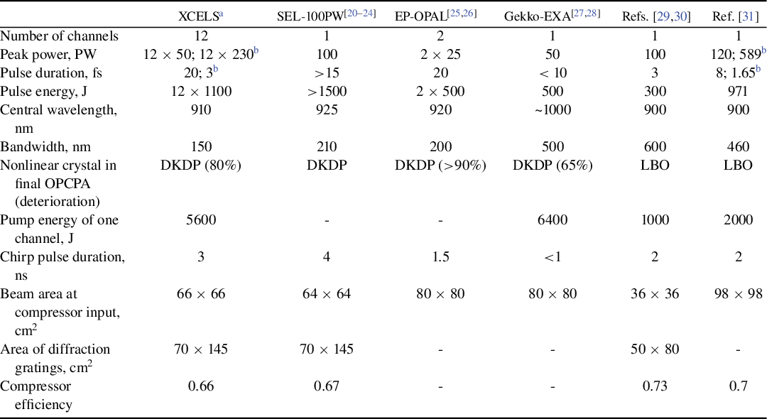
a For maximum grating size.
b After post-compression.
The layout of the XCELS laser is shown in Figure 1. The frontend generates chirped femtosecond pulses at a wavelength of 910 nm and nanosecond pulses at 1054 nm injected into the OPCPA pump lasers, and also ensures the all-optical synchronization of these pulses as well as the required energy and spatiotemporal parameters. An intermediate OPCPA operating at a relatively high (1 Hz) repetition rate amplifies the pulse to tens of joules. Booster OPCPA already provides a beam with kilojoule energy, which is divided into 12 beams. In the final 12 OPCPAs, the 12 chirped pulses are each amplified to the kilojoule level, after which they are compressed to 20 fs (the Fourier-transform-limited pulse width being 17 fs) by 12 grating compressors (GCs). Thus, the XCELS laser will have 12 identical channels, each generating a pulse with power of 50 PW and maximum focal intensity of 0.44 × 1025 W/cm2, assuming an ideal focus (Strehl number = 1) with an F/1 focusing optics. All 12 beams are directed to the main target chamber, in which they are focused in a dipole geometry with the focal intensity of almost 1026 W/cm2. The pulses are assumed to be coherently combined, which will increase the focal intensity to 3.2 × 1026 W/cm2. In addition to the main target chamber, the XCELS project includes up to 10 user laboratories, each receiving one or more beams for experiments. The laboratories will be equipped with a variety of experimental instrumentation, including an accelerator of electrons. Table 2 presents the main parameters of the laser pulse at all key points of the XCELS laser, marked in Figure 1 by yellow asterisks.
General block diagram of the XCELS laser. DKDP_i, nonlinear crystal in intermediate OPCPA; DKDP_0, nonlinear crystal in booster OPCPA; DKDP_1–12, nonlinear crystals in final OPCPAs; GC, grating compressor.

Main parameters at key points of the XCELS laser.

It should also be noted that in the last few years, the method of additional compression (post-compression) of ultrahigh-power laser pulses after the GC has been developed[ Reference Mourou, Mironov, Khazanov and Sergeev 32 – Reference Khazanov, Mironov and Mourou 34 ]. The essence of the method is to broaden the spectrum during propagation in a cubic-nonlinear medium and subsequently compress the pulse using chirped (dispersive) mirrors. The use of post-compression will allow increasing both the power and the focal intensity of the pulse in each channel of the XCELS laser by several times (see Section 2.10).
A proposed layout of the building for the XCELS is shown in Figure 2. The total area is more than 24,000 m2, including 7100 m2 of ISO 7 class, 11 m high, and 200 m2 of ISO 5 class, 4.5 m high. There are three airlock chambers: for large equipment, for standard equipment and for personnel. The premises of the main floor are divided into several zones with different cleanliness classes: the frontend (1) and the intermediate OPCPA (2); the pump laser for wide-aperture OPCPAs (3); the booster (4) and final (5) OPCPAs; the transport telescopes and optical compressors (6); the main target chamber (7); the experimental laboratories (8). Electric energy storage, vacuum pumps, water treatment, ventilation and air conditioning systems are located in the basement. There are also auxiliary facilities foreseen (nitrogen station, compressor and gas bottle storage, etc.). The total consumed electrical power is about 7.5 MW. The building has an internal hollow monolithic frame and an external part, standing on two decoupled foundations. The vacuum and other systems, which may cause vibrations, are installed on vibration-isolated foundations. Vibration and shock loads in the frequency range of 1–200 Hz, transmitted through foundations and supports, do not cause vibrations of the facility structures with an amplitude of more than 10–10 g2/Hz. Inside the laser hall, a network of geodesic reference marks is provided to systematically monitor the drift of both the building foundation and equipment.
General view of the building for the XCELS project: frontend (1); intermediate OPCPA (2); pumping zone for wide-aperture OPCPAs (3); booster OPCPA (4); final OPCPAs (5); transport telescopes and optical compressors (6); main target chamber (7); experimental laboratories (8).

A detailed description of the XCELS laser is presented below in Section 2, and an overview of the experiments planned at the XCELS facility is given in Section 3. Finally, conclusions are drawn in Section 4.
2 eXawatt Center for Extreme Light Studies laser
This part describes the layout, input and output parameters, principles of construction and interconnection of all components of the XCELS laser facility complex. The general schematic diagram and pulse parameters at all key points of the laser are presented in Figure 1 and Table 2, respectively.
2.1 Frontend
The frontend generates pulses injected into the pump laser amplifiers (points 1.1 and 1.2 in Figure 1) and a broadband signal pulse directed to a chain of parametric amplifiers (point 1.3 in Figure 1). For stable operation of parametric amplifiers, optical synchronization of these pulses is necessary. The parameters of the pulse injected into the pump lasers must be variable to allow the gain optimization and to control the output pulse shape of the pump lasers. This provides flexibility in the design and operation of the entire XCELS laser complex. The frontend is thoroughly discussed in Ref. [Reference Mukhin, Soloviev, Perevezentsev, Shaykin, Ginzburg, Kuzmin, Mart'yanov, Shaikin, Kuzmin, Mironov, Yakovlev and Khazanov35], and here we confine ourselves to a brief description. The frontend consists of three parts: fiber, solid state and parametric (Figure 3).
Schematic diagram of the frontend. MO, master oscillator; NF, nonlinear fiber; FA, fiber amplifier; FRA, fiber regenerative amplifier; FSRA, femtosecond regenerative amplifier; DRA, disk regenerative amplifier; DMA, disk multipass amplifier; NA, neodymium amplifier; YA, ytterbium amplifier; WLG, white light generator; FOPA, parametric amplifier; XPW, orthogonal polarization generator; GS, stretcher on diffraction grating; AOPDF, acousto-optical programmable dispersion filter.

The master oscillator is a femtosecond ytterbium fiber laser (wavelength ~1030 nm, pulse repetition rate of several tens of megahertz) synchronized with an external frequency standard, which makes it possible to synchronize all devices necessary for experiments with the output pulses of the XCELS laser. The oscillator pulse is divided into two. The first part is stretched in a fiber Bragg grating stretcher and amplified in a fiber amplifier to an energy of tens of nanojoules, after which it is divided into three replicas. To accurately adjust the time delay, each replica has delay lines based on a piezoelectric disk, which mechanically stretches out the fiber coiled and glued on its side[ Reference Zelenogorskii, Andrianov, Gacheva, Gelikonov, Krasilnikov, Mart'yanov, Mironov, Potemkin, Syresin, Stephan and Khazanov 36 ] (not shown in Figure 3) when a proper voltage is applied to the disk. Two replicas are used in ytterbium amplifiers in the solid-state part (Figure 3), and the third one is used as an auxiliary output (point 1.5). The second part of the master oscillator beam passes through a nonlinear fiber, which broadens the pulse spectrum so that it overlaps the gain range in neodymium glass. Next, the pulse is divided into four replicas, each of which is amplified to tens of nanojoules in a fiber regenerative amplifier. A chirped fiber Bragg grating is used as one of the amplifier mirrors. Its transmission spectrum determines the central wavelength (1054 or 1030 nm) and the spectral width (2 nm) at the amplifier output. Multiple reflections from the grating with a dispersion of 200 ps/nm will ensure the necessary stretch even for narrow-band signals and allow relatively smooth control of the pulse duration with a spectral width of 1 nm due to the varying number of roundtrips of the regenerative amplifier. Then one of the four beams is sent to the auxiliary output (point 1.4), while the other three enter the solid-state part.
In the solid-state part (Figure 3(b)), optimal temporal and spatial profiles of the laser pulses are formed, and the pulses are also amplified to the required energies. A femtosecond regenerative Yb amplifier[ Reference Kuznetsov, Mukhin and Palashov 37 , Reference Soloviev, Burdonov, Chen, Eremeev, Korzhimanov, Pokrovskiy, Pikuz, Revet, Sladkov, Ginzburg, Khazanov, Kuzmin, Osmanov, Shaikin, Shaykin, Yakovlev, Pikuz, Starodubtsev and Fuchs 38 ] amplifies the pulse to a millijoule energy level while maintaining a subpicosecond duration. This pulse is used in the parametric part to generate a pulse at a wavelength of 910 nm. In the ytterbium disk regenerative amplifier similar to that described in Ref. [Reference Soloviev, Burdonov, Ginzburg, Gonoskov, Katin, Kim, Kirsanov, Korzhimanov, Kostyukov, Lozhkarev, Luchinin, Mal'shakov, Martyanov, Nerush, Palashov, Poteomkin, Sergeev, Shaykin, Starodubtsev, Yakovlev, Zelenogorsky and Khazanov39], the pulse is amplified to an energy of 200 mJ at a repetition rate of 1 kHz and then compressed to 10 ps. The main part of the pulse (energy 180 mJ) after frequency doubling is used as a pump for frequency domain optical parametric amplification (FOPA)[ Reference Schmidt, Thire, Boivin, Laramee, Poitras, Lebrun, Ozaki, Ibrahim and Legare 40 ]. The rest of the pulse (energy 20 mJ) is stretched to 3.5 ns in the grating stretcher GS1 and amplified to an energy slightly less than 1 J in a multipass disk amplifier at a repetition rate of approximately 100 Hz. This pulse, after frequency doubling, is used to pump the OPCPA in the parametric part of the frontend. The temporal profile of the amplified laser pulses in the Yb amplifiers is close to Gaussian. The spatial profile of the laser beam after the disc amplifier is transformed into super-Gaussian[ Reference Khiar, Revet, Ciardi, Burdonov, Filippov, Béard, Cerchez, Chen, Gangolf, Makarov, Ouillé, Safronova, Skobelev, Soloviev, Starodubtsev, Willi, Pikuz and Fuchs 41 ].
Two neodymium and one ytterbium amplifiers provide injection pulses into the power amplifiers (points 1.1 and 1.2 in Figure 3). One of the neodymium amplifiers is used to inject a pulse into the pump laser of the OPCPA final stages. Several options are considered as the pump laser for the intermediate OPCPA (see Section 2.2 for more details). To ensure the flexibility of the frontend, two options, neodymium and ytterbium, are implemented at output 1.2. Before amplification, the pulses are profiled to provide the necessary (close to rectangular) shape of the pump pulse of the intermediate, booster and final parametric amplifiers. Since the pulses are chirped, it is convenient to use the spectral approach for their profiling[ Reference Mironov, Poteomkin, Gacheva, Andrianov, Zelenogorskii, Krasilnikov, Stephan and Khazanov 42 , Reference Kuzmin, Mironov, Gacheva, Zelenogorsky, Potemkin, Khazanov, Kanareykin, Antipov, Krasilnikov and Loisch 43 ]. This approach allows tuning the delay in few ps range with approximately kHz resolution to suppress a temporal jitter on ps parametric stages. After profiling, all three pulses are amplified to an energy of 100 mJ, first in regenerative and then in neodymium glass and ytterbium-doped yttrium aluminum garnet (Yb:YAG) crystal rod amplifiers. The diode pumping of these amplifiers makes it possible to operate at a pulse repetition rate of 10 Hz.
In the parametric part (Figure 3), a pulse from a femtosecond regenerative amplifier is used as a signal pulse. Similar to Refs. [Reference Chen, Farhat, Askarpour, Tymchenko and Alù44,Reference Mukhin, Volkov, Vikulov, Perevezentsev and Palashov45], with the help of supercontinuum generation, the beam is converted into the wavelength band of 700–1000 nm with a Fourier-transform-limited pulse duration of several cycles and with passive stabilization of the field phase relative to the envelope, also known as CEP-stability. Experiments[ Reference Mukhin, Glushkov, Soloviev, Shaikin, Ginzburg, Kuzmin, Martyanov, Stukachev, Mironov, Yakovlev and Khazanov 46 ] showed the possibility of generating laser pulses with a duration of 20 fs in the band of parametric amplification in a DKDP crystal (Figure 4).
Measured pulse intensity and phase at the output of a parametric amplifier based on a BBO crystal[ Reference Mukhin, Glushkov, Soloviev, Shaikin, Ginzburg, Kuzmin, Martyanov, Stukachev, Mironov, Yakovlev and Khazanov 46 ].

Next, the pulse is parametrically amplified in a beta barium borate (BBO) crystal using FOPA[ Reference Schmidt, Thire, Boivin, Laramee, Poitras, Lebrun, Ozaki, Ibrahim and Legare 40 ], which makes it possible to eliminate the stretcher and compressor at this stage of amplification. The second harmonic of the pulse from a disk regenerative amplifier is used for pumping. The energy of the amplified pulse is about 18 mJ. Then, one half of the beam is directed to auxiliary output 1.6 (Figure 3), and the other half is directed to the next amplification stages after contrast enhancement by means of orthogonal polarization generation[ Reference Jullien, Albert, Burgy, Hamoniaux, Rousseau, Chambaret, Augé-Rochereau, Chériaux, Etchepare, Minkovski and Saltiel 47 ] or a nonlinear interferometer[ Reference Khazanov and Mironov 48 – Reference Silin and Khazanov 50 ]. Before amplifying, this pulse is stretched by a stretcher based on diffraction gratings to a duration of 3 ns, which is determined by the compressor (see Section 2.6 for more details). The acousto-optical programmable dispersion filter[ Reference Tournois 51 ] optimizes the spectral phase (and, if necessary, the amplitude) to achieve a Fourier-transform-limited pulse duration after the compressor. After the filter, the pulse enters the parametric amplifier and is incident on the DKDP crystal. The energy of the pump pulse (the second harmonic of the disk multipass amplifier) is 500 mJ, and the efficiency of the parametric amplifier is 30%. Thus, a pulse with an energy of 150 mJ and a repetition rate of 100 Hz is sent to the XCELS intermediate parametric amplifier (point 1.3).
2.2 The intermediate OPCPA
The OPCPA in the DKDP crystal is the base of the XCELS laser. In Ref. [Reference Lozhkarev, Freidman, Ginzburg, Khazanov, Palashov, Sergeev and Yakovlev10], the dependence of the refractive index of this crystal on the wave frequency (the Sellmeier formula) was determined for an arbitrary degree of deuteration and it was found that, when pumped by the second harmonic of a neodymium laser at the central wavelength of an amplified pulse of 910 nm, ultra-wideband phase matching exists. Further studies[ Reference Li and Kawanaka 30 , Reference Galimberti, Hernandez-Gomez, Musgrave, Ross and Winstone 52 – Reference Zhu, Zhang, Xu, Liu, Ji, Zhang, Zhou, Liu, Wang and Sun 56 ] confirmed these results and showed the prospectivity of using a DKDP crystal for broadband OPCPA. In combination with the ability to grow a crystal with an aperture of tens of centimeters, this provides a unique opportunity to transfer energy from a narrow-band neodymium laser pulse to a broadband chirped pulse that can be compressed down to 10–20 fs. It is no coincidence that the petawatt power level of OPCPA has been obtained using only this crystal[ Reference Lozhkarev, Freidman, Ginzburg, Katin, Khazanov, Kirsanov, Luchinin, Mal'shakov, Martyanov, Palashov, Poteomkin, Sergeev, Shaykin and Yakovlev 14 , Reference Belov, Buchirina, Voronich, Voronina, Garanin, Dolgopolov, Zimalin, Kedrov, Koltygin, Litvin, L'vov, Manachinsky, Markov, Mecheryakov, Ogorodnikov, Romanov, Rukavishnikov, Rukavishnikov, Savkin, Senik, Sukharev, Trikanova, Tytin, Filatova, Chernov, Ginzburg, Katin, Kirsanov, Lozhkarev, Luchinin, Mal'shakov, Martyanov, Palashov, Poteomkin, Sergeev, Freidman, Khazanov, Shaykin and Yakovlev 15 , Reference Zhu, Xie, Sun, Kang, Yang, Guo, Zhu, Zhu, Gao, Liang, Cui, Yang, Zhang and Lin 57 ], and most of the facilities currently being designed with a peak power of about 100 PW are also based on OPCPA in a DKDP crystal (see Table 1). This indispensability of the DKDP crystal manifests itself in full measure in the booster and final OPCPAs (Figure 1), where the beam apertures are 25 cm or more. In the intermediate amplifier, the beam diameter is 10 cm and, in principle, a lithium triborate (LBO) crystal[ Reference Wang, Yu, Wu and Boughton 58 ] can be used, but the gain band in it is shifted towards short wavelengths[ Reference Li, Leng and Li 5 ]. As the degree of deuteration of the DKDP crystal decreases, the center of the gain band shifts to the long wavelength region, closer to degenerate phase matching; the band width increases, but the idler wave absorption also increases[ Reference Hu, Wang, Xu, Yu, Wu, Zhang, Yang, Ji, Bai, Liang, Leng and Li 55 , Reference Zhu, Zhang, Xu, Liu, Ji, Zhang, Zhou, Liu, Wang and Sun 56 ]. For the required spectral width of 150 nm (see Section 2.6), the deuteration degree of 80% seems to be optimal. The surfaces of the DKDP crystals are sol–gel coated to protect against moisture and reduce Fresnel losses.
The pulse energy in OPCPA is limited by the threshold of DKDP crystal breakdown by the pump pulse. The DKDP crystal breakdown threshold at a wavelength of 1053 nm for a 3-ns pulse exceeds 7 GW/cm2[ Reference Cai, Lin, Li, Lu and Zheng 59 ]. KDP (KH2PO4) crystals are used in the UFL-2M laser facility for frequency doubling; the intensity of the second harmonic is about 3 GW/cm2 in a pulse with a duration of about 3 ns[ Reference Garanin, Bel’kov and Bondarenko 60 , Reference Derkach, Derkach and Zhukov 61 ]. The optical resistance of DKDP crystals may be lower than that of KDP crystals, and the resistance at the second harmonic is lower than at the fundamental one, so we consider the OPCPA pump intensity of 1.5 GW/cm2 to be safe. This pump intensity is used for all XCELS laser parametric amplifiers. It is worth mentioning that cubic nonlinearity in OPCPA is almost negligible because at the intensity of 1.5 GW/cm2 the B-integral is about 0.5, even for 10 cm DKDP crystal length.
Our long-term experience of working with OPCPA[ Reference Lozhkarev, Freidman, Ginzburg, Khazanov, Palashov, Sergeev and Yakovlev 10 , Reference Lozhkarev, Garanin, Gerke, Ginzburg, Katin, Kirsanov, Luchinin, Mal'shakov, Martyanov, Palashov, Poteomkin, Rukavishnikov, Sergeev, Sukharev, Khazanov, Freidman, Charukhchev, Shaykin and Yakovlev 13 – Reference Belov, Buchirina, Voronich, Voronina, Garanin, Dolgopolov, Zimalin, Kedrov, Koltygin, Litvin, L'vov, Manachinsky, Markov, Mecheryakov, Ogorodnikov, Romanov, Rukavishnikov, Rukavishnikov, Savkin, Senik, Sukharev, Trikanova, Tytin, Filatova, Chernov, Ginzburg, Katin, Kirsanov, Lozhkarev, Luchinin, Mal'shakov, Martyanov, Palashov, Poteomkin, Sergeev, Freidman, Khazanov, Shaykin and Yakovlev 15 ] showed that the efficiency of a parametric amplifier (the amplified pulse energy normalized to the pump pulse energy) in the experiment turns out to be 15%–25% lower than the theoretical one. This may be due to pump beam inhomogeneity, synchronization or alignment inaccuracy, poor antireflection, etc. In the framework of this work, we took into account this experience for all OPCPAs as follows: the theoretically calculated efficiency and output pulse energy were multiplied by a safety factor equal to 0.75.
The intermediate OPCPA is the last amplifier pumped by the non-kilojoule UFL-2M laser (Figure 1), so it performs two important functions. Firstly, to use the kilojoule pump of the booster OPCPA efficiently, the intermediate OPCPA must amplify the pulse to an energy of tens of joules. This requires a pump pulse energy of at least 100 J with a quasi-rectangular pulse duration of 3.5 ns, which ensures overlap between the pump pulse and the 3-ns chirped pulse. The quasi-rectangular shape of the pulse is provided by profiling the output pulse[ Reference Mironov, Poteomkin, Gacheva, Andrianov, Zelenogorskii, Krasilnikov, Stephan and Khazanov 42 , Reference Kuzmin, Mironov, Gacheva, Zelenogorsky, Potemkin, Khazanov, Kanareykin, Antipov, Krasilnikov and Loisch 43 ] in the frontend (point 1.2 in Figures 1 and 3). Secondly, the intermediate OPCPA ensures the operation of the XCELS laser with a multipetawatt power and a repetition rate significantly higher than two pulses per day (point 2.2 in Figure 1). Both the energy and the pulse repetition rate at the output of the OPCPA are determined by the respective parameters of the pump laser, and here a compromise is required between the repetition rate and energy, which, in turn, are determined by the active elements used. Three options can be distinguished: lamp-pumped neodymium glass rod lasers[ Reference Poteomkin, Khazanov, Martyanov, Kirsanov and Shaykin 62 , Reference Shaykin, Kuzmin, Shaikin, Burdonov and Khazanov 63 ], lamp-pumped neodymium glass active mirrors[ 64 ] and diode-pumped Yb:YAG cryogenic disk lasers[ Reference Divoký, Pilař, Hanuš, Navrátil, Denk, Severová, Mason, Butcher, Banerjee, De Vido, Edwards, Collier, Smrž and Mocek 65 ]. These options differ from each other by two orders of magnitude in terms of the pulse repetition rate (Table 3). There are also significant differences in the energy, pulse duration, dimensions, cost, etc. Let us consider all the three options.
Five options of intermediate OPCPA (optical schemes are shown in Figures 5(a)–5(e)).

a Multiplied by a safety factor equal to 0.75 (see text).
Rod lasers consist of a series of Nd:glass amplifiers with active element diameters increasing to 100 mm in the last amplifier. The pulse energy is mainly limited by small-scale self-focusing[ Reference Poteomkin, Martyanov, Kochetkova and Khazanov 66 ]. In Ref. [Reference Shaykin, Kuzmin, Shaikin, Burdonov and Khazanov63], an output energy of 500 J was obtained upon amplifying two successive pulses with a duration of 1 ns. Thus, at a pulse duration of 3.5 ns, the laser will have an almost twofold margin in terms of damage resistance, and the antireflection coating of the amplifier rods will increase the energy to 550 J. After conversion to the second harmonic with an efficiency of 75%, the energy in the pump pulse will be more than 400 J. This ensures at the output of one OPCPA (Figure 5(a)) the pulse energy of almost 150 J and the power after the compressor of almost 5 PW (Table 3). Figure 6(a) presents the pulse spectra at the input and output of the OPCPA, and also shows the dependence of the energy at the output of the intermediate OPCPA on the thickness of the DKDP crystal. Obviously, rod lasers are the simplest, most reliable and cheapest option for OPCPA pumping; however, the pulse repetition rate is only 0.001 Hz due to the low thermal conductivity of the glass and the large rod radius, as well as due to the lamp pumping.
Variants of the optical scheme of the intermediate OPCPA when pumped by a lamp-pumped neodymium glass rod laser (a), a lamp-pumped neodymium glass active-mirror laser (b), (c) and two diode-pumped Yb:YAG cryogenic disk lasers (d), (e) (see also Table 3).

Signal spectra at the input (black curves) and at the output (red curves) of OPCPA and the shape of the pump pulse (green curves) for the five options shown in Figure 5 and Table 3. The insets show the dependence of the energy W on the thickness L of the DKDP crystal. The dashed curves in (b), (d) and (e) show the corresponding dependence for the first OPCPA cascade.

The pulse repetition rate (0.1 Hz) is significantly higher for lasers based on active Nd:glass mirrors due to the fact that the time of heat removal is determined by the small thickness of the mirror, and also due to the longitudinal temperature gradient, which is much less dangerous than the transverse one. For estimation, we take the Premiumlite GLASS laser (Amplitude Laser Group) with an energy of 260 J and a pulse duration of 15 ns[ 64 ]. Based on conservative estimates (the pulse energy is limited by the optical breakdown and is proportional to the root of the pulse duration), for a pulse duration of 3.5 ns, the energy will be only 130 J, which is clearly not enough to pump the intermediate OPCPA. At the same time, with a pulse duration of 7 ns, the energy will be about 200 J, which can be converted to 50 J at the OPCPA output by complicating the setups, namely, by using either second harmonic generation (SHG) with pulse shortening and standard OPCPA (Figure 5(b)), or standard SHG and two-stage OPCPA pumped by 7-ns pulses (Figure 5(c)). In the first case, the SHG uses the eoe-type interaction of the first half of the pulse delayed by 3.5 ns with the second half of the same pulse. In the second case, two halves of a 7-ns pulse pump two successive OPCPA stages. Figures 6(b) and 6(c) show the dependences of the energy at the OPCPA output on the thickness of the DKDP crystal(s).
Thermal effects are most strongly suppressed in cryogenic lasers based on Yb:YAG crystals with diode pumping. The leader is the DiPOLE laser[ Reference Divoký, Pilař, Hanuš, Navrátil, Denk, Severová, Mason, Butcher, Banerjee, De Vido, Edwards, Collier, Smrž and Mocek 65 ], which provides an energy of more than 150 J in a 10-ns pulse at a repetition rate of 10 Hz. Recalculating for a pulse duration of 7 ns, we obtain an energy of about 125 J. In this case, two such lasers are needed to pump the intermediate OPCPA, and the setup becomes even more complicated. Either SHG with pulse shortening and two standard OPCPA stages is used in each of the lasers (Figure 5(d)), or SHG of beams from two lasers and a two-stage OPCPA pumped by 7-ns pulses is used (Figure 5(e)). From Figures 6(d) and 6(e), as well as from Table 3, it can be seen that the energy and power of the output pulse are approximately the same as in the case of using a single laser with active mirrors. The disadvantages of Yb:YAG crystal lasers include not only the setup complication, but also a significantly higher cost. In addition, it is important to note that the thermal effects in the DKDP crystal associated with idler wave absorption will limit the pulse repetition rate. This problem can be solved by using LBO crystals.
Thus, each of the three variants of the intermediate OPCPA pump laser considered has its own advantages and disadvantages. The most promising is the creation of two complementary options, for example, those shown in Figures 5(a) and 5(e). It is worth emphasizing that output XCELS peak power at relatively high repetition rate is between 1.7 and 4.9 PW, depending on the intermediate OPCPA pump laser (Table 3).
After OPCPA, the beam diameter is increased to 25 cm using a telescope and the beam is directed either to the input of the booster OPCPA (point 2.1 in Figure 1), or to the compressor (point 5.1 in Figure 1). The telescope consists of two confocal spherical mirrors and also performs the function of cleaning the beam of spatial noise.
2.3 Pumping of the booster and final OPCPAs
To provide an energy of 1 kJ or more at the output of the booster amplifier and 12 final parametric amplifiers, 13 pump pulses with an energy of several kilojoules each at a wavelength of about 0.5 μm are required, with the laser pulse duration being 3.5 ns. At the current level of development of laser technology, this is feasible only in Nd:glass lasers followed by SHG. Despite great progress in diode pumping technology, such energy is available using lamp pumping only. Nanosecond neodymium glass lasers are used for research in the field of inertial confinement fusion[ Reference Edwards and Danson 67 ]. The leading position belongs to the NIF megajoule facility in the USA, which has been operating since 2012[ Reference Spaeth, Manes, Kalantar, Miller, Heebner, Bliss, Speck, Parham, Whitman, Wegner, Baisden, Menapace, Bowers, Cohen, Suratwala, Nicola, Newton, Adams, Trenholme and Zacharias 68 ]. Similar facilities are under construction in France[ Reference Miquel, Batani and Blanchot 69 ], China and also in Russia (UFL-2M facility in Sarov)[ Reference Garanin, Bel’kov and Bondarenko 60 , Reference Derkach, Derkach and Zhukov 61 , Reference Garanin 70 ].
The active elements in such lasers are slabs positioned at the Brewster angle. To use the energy of the pump lamps more efficiently, the beams have a square cross-section, and the laser channels are grouped into modules of four or eight pieces each. The UFL-2M prototype, the Luch four-channel facility[ Reference Garanin, Zaretskii, Il'kaev, Kirillov, Kochemasov, Kurunov, Murugov and Sukharev 11 ], was successfully used to pump a DKDP crystal parametric amplifier in a petawatt laser[ Reference Belov, Buchirina, Voronich, Voronina, Garanin, Dolgopolov, Zimalin, Kedrov, Koltygin, Litvin, L'vov, Manachinsky, Markov, Mecheryakov, Ogorodnikov, Romanov, Rukavishnikov, Rukavishnikov, Savkin, Senik, Sukharev, Trikanova, Tytin, Filatova, Chernov, Ginzburg, Katin, Kirsanov, Lozhkarev, Luchinin, Mal'shakov, Martyanov, Palashov, Poteomkin, Sergeev, Freidman, Khazanov, Shaykin and Yakovlev 15 ], and the XCELS laser will use two eight-channel modules similar to the UFL-2M modules. Thirteen channels will be used to pump the booster OPCPA and 12 final OPCPAs (Figure 1); the remaining three will be used as independent sources of nanosecond kilojoule pulses required in many experiments.
A schematic diagram of the power section of the UFL-2M facility is shown in Figure 7 [ Reference Garanin 70 ]: four passes through two sequential multislab amplifiers are provided by a reverser based on Pockels cells with plasma electrodes. The power part of the UFL-2M modules can be used without changes, and the necessary time and energy parameters of the output pulse are provided by the frontend (see Section 2.1). In contrast to the UFL-2M, the shape of the output pulse should be close to rectangular, for example, 10th-order super-Gaussian. The pump pulse energy of the final OPCPAs required for the XCELS laser depends on the size of the diffraction gratings used in the compressor. For gratings with the minimum size of 57 cm × 101 cm, an energy of about 4 kJ is required, and for gratings with a size of 70 cm × 145 cm, about 6 kJ is required (see Sections 2.5 and 2.6). The energy at the output of one UFL-2M channel exceeds these values[ Reference Garanin, Bel’kov and Bondarenko 60 , Reference Derkach, Derkach and Zhukov 61 ], which will allow operating the pump laser of the final OPCPAs with parameters below the limit ones.
Optical layout of one channel of the UFL-2M setup[ Reference Garanin 70 ].

The spatial beam profile at the output of the UFL-2M channel is close to uniform, which is optimal for OPCPA pumping. The beam size must be optimized to ensure efficient nonlinear interaction in DKDP crystals (see Sections 2.4 and 2.5). Since the pump pulse is narrow-band, a lens telescope can be used for this. The telescope can be a compact Euler or a Keplerian one, which relays the image to the input of the DKDP crystal and cleans the beam of spatial noise.
2.4 Booster OPCPA
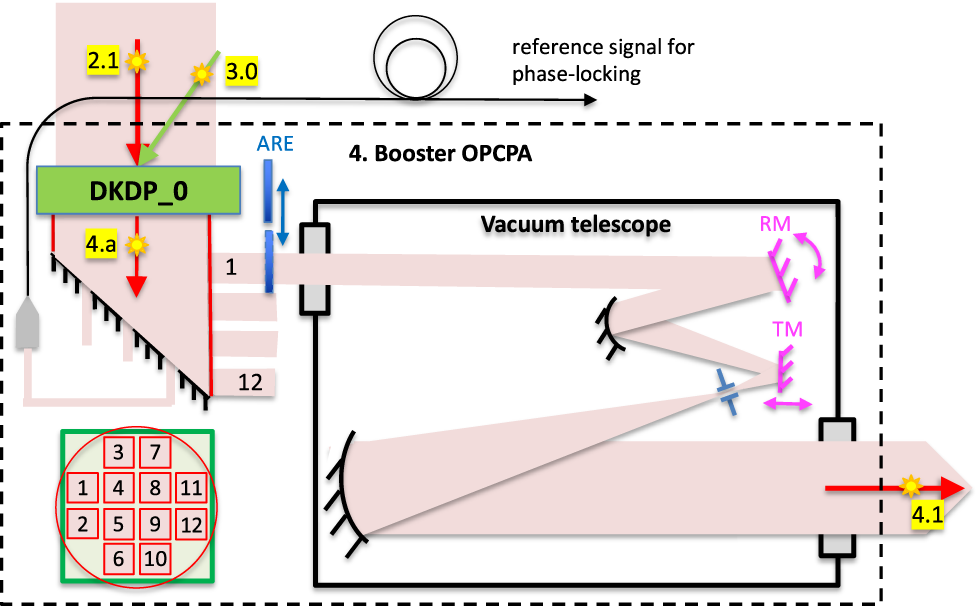
The energies of the output pulses (Table 2) of the booster and final OPCPAs require the use of DKDP crystals with an aperture of 25 cm or more. Technology makes it possible to grow such crystals. However, the optical quality of crystals deteriorates with an increase in both their aperture and thickness, making it important to minimize all sizes of crystals used in these OPCPAs. The DKDP crystal aperture is limited (from below) by the ratio of the minimum required pump energy (the output pulse energy divided by the OPCPA efficiency) to the maximum allowable pump energy density, which depends on the optical breakdown of the DKDP crystal and equals 5.3 J/cm2 for a pulse duration of 3.5 ns (see Section 2.2). The smaller the thickness of the DKDP crystal, the greater the energy of the input pulse. Thus, to reduce the crystal size, it is necessary to increase not only the OPCPA efficiency, but also the input pulse energy. For the final OPCPAs, an input energy of about 50 J seems reasonable. The pulse energy after the intermediate OPCPA satisfies this requirement; however, when divided into 12 channels, the energy decreases, so one more OPCPA, a booster one, is needed before beam splitting (Figures 1 and 8). At the output of the booster OPCPA, the pulse energy exceeds 1 kJ, which determines the pump pulse energy and the aperture of the DKDP crystal. The DKDP crystal thickness is determined by the energy of the input pulse, which depends on the used version of the intermediate OPCPA pump laser (Table 3) and ranges from 3.8 to 4.3 cm. The parameters of the booster OPCPA are summarized in Table 4 and illustrated in Figure 9. A specific feature of the booster OPCPA is that the input beams have different transverse shapes: the pump beam is square, and the signal beam is round. Moreover, in the subsequent division into 12 square beams (see below), only a part of the signal beam aperture is used.
Booster OPCPA. ARE, auxiliary removable equipment (filters, diaphragms, screens); TM, a mirror on the translator; RM, a rotating mirror, used for alignment and phasing of channels (see Sections 2.8 and 2.9). In the lower left corner there is a diagram of the beam division into 12 replicas (the green square is the pump beam cross-section, the red circle is the signal beam cross-section); one telescope out of twelve is shown.
Booster OPCPA parameters. All apertures and energies (except for the total pump energy) refer to the homogeneous region of the beam; total aperture is approximately 20% larger.

a Multiplied by a safety factor equal to 0.75 (see text).
b For different variants of the intermediate OPCPA pump.
Signal spectra at the input (black curve) and output (red curve) of OPCPA and the pump pulse shape (green curve) for booster OPCPA. The inset shows the dependence of the energy W on the thickness L of the DKDP crystal.

After dividing the beam into 12 channels for their subsequent phasing, it is important that the number of elements in the main target chamber up to the focal plane is as small as possible and that the elements in each channel are as similar as possible (preferably identical). In this regard, beam splitting using semitransparent mirrors or polarizers is unpromising, and it is preferable to ‘cut out’ 12 square replicas from the beam aperture, as shown in the lower left corner of Figure 8. To avoid diffraction at the edges of ‘cut’ beams, either soft diaphragms are used, similar to those described in Refs. [Reference Kryzhanovskiĭ, Sedov, Serebryakov, Tsvetkov and Yashin71,Reference Martyanov, Poteomkin, Shaykin and Khazanov72], or mirrors with an inhomogeneous reflection coefficient, or toothed diaphragms[ Reference Sizova, Moskalev and Mikheev 73 , Reference Bel’kov, Voronich, Garanin and Zimalin 74 ]. The pulse energy density is about 2 J/cm2, which makes it possible to use such diaphragms[ Reference Bel’kov, Voronich, Garanin and Zimalin 74 ]. Each of the 12 beams is 6 cm × 6 cm in size. The 5 cm × 5 cm region of uniform intensity contains about 50 J of energy. The peripheral region (0.5 cm on each side) will have little to no enhancement in the final OPCPA, as the pump intensity in this region is low. Further, the size of the homogeneous region of the beam is increased using a Keplerian telescope located in a vacuum with a magnification of 5 or 6 to the size required in the final OPCPA of 25 cm × 25 cm or 30 cm × 30 cm, respectively (see Section 2.5 and Table 2).
The telescope consists of two off-axis parabolic mirrors and one flat mirror on a translator located not far from the waist. To preserve the uniformity of the intensity distribution over the beam cross-section, the angles of incidence on the parabolic mirrors must be equal and lie in the same plane, as shown in Figure 8. The mirror on the translator is moved along the z-axis with the help of piezoceramics and is used for channel phase-locking (see Section 2.9). This requires a mirror with as little mass as possible, so it is located as close to the waist as its optical stability allows. For a mirror aperture of 2 cm × 2 cm, the energy density is about 13 J/cm2. The telescope also performs the function of a spatial filter, cleaning the beam of high-frequency noise by means of a diaphragm located in the focal plane. Since a high level of noise is inevitable after the beam splitter, the requirements for filtering efficiency are especially high. That is why the telescope uses parabolic (rather than spherical) mirrors, which ensure the minimum size of the beam in the waist and, accordingly, the minimum size of the diaphragm. In addition, a diaphragm is used, if necessary, to protect the laser from a spurious beam traveling in the opposite direction from the main target chamber (see Section 2.7). To do this, with the help of an auxiliary pulse incident on the diaphragm after the main one, a plasma is formed in the waist, which scatters the backward propagating pulse arriving with a delay equal to the time of flight to the focus in the main target chamber and back, about 600 ns.
2.5 Twelve final OPCPAs
The final OPCPAs provide maximum beam energy. The pulse energy at the output of one XCELS channel is limited by the diffraction gratings of the compressor (see Section 2.6). These limits determine the energy required at the output of the final OPCPA. The corresponding values are given in Tables 2 and 5 for two variants of diffraction gratings. For the widest-aperture gratings, the required pump pulse energy is about 6 kJ, which is less than the maximum output energy of the UFL-2M channel, that is, the pump energy of the final OPCPAs can be considered unlimited. As noted in Section 2.2, the DKDP crystal optical breakdown limits the energy density, and the safe value is 5.3 J/cm2 (intensity of 1.5 GW/cm2). This value determines the beam aperture in the DKDP crystal, which, depending on the grating size, is 25 or 30 cm. The crystal thickness is the same for both cases and equals 4.3 cm. Figure 10 shows the dependence of the amplified pulse energy on the DKDP crystal thickness, as well as the pulse spectra at the input and output of OPCPA.
Signal spectra at the input (black curve) and output (red curve) of OPCPA and the pump pulse shape (green curve) for the final OPCPA. The inset shows the dependence of the energy W on the thickness L of the DKDP crystal.

Final OPCPA parameters for two options. All apertures and energies (except for the total pump energy) refer to the homogeneous region of the beam; the full aperture is about 20% larger.

a Multiplied by a safety factor equal to 0.75 (see text).
The quality of DKDP crystals noticeably worsens with increasing aperture, so it is of interest to increase the pump intensity above 1.5 GW/cm2, which will allow reducing both the transverse and the longitudinal crystal sizes in proportion to the intensity square root, that is, the crystal volume is proportional to the pump intensity to the power of –3/2. As noted in Section 2.2, the value of 1.5 GW/cm2 is determined with a margin and, possibly, it can be increased. To determine how far one can go along this path, additional studies of the optical damage threshold of the DKDP crystal are needed.
2.6 Twelve compressors
The compressors of all superhigh-power lasers are based on the Tracy scheme[ Reference Treacy 75 ] (Figure 11), in which the necessary chirped pulse compression factor is provided by the properties of the diffraction gratings, primarily by second-order dispersion (group velocity dispersion). Since the dispersions in the compressor and in the stretcher have opposite signs, they compensate each other and make it possible to stretch and compress the pulses almost to the original duration. To obtain the minimum (Fourier-transform-limited) duration of femtosecond pulses, a precise control of both the group velocity dispersion and the higher-order dispersions is required. For this purpose, an acousto-optic programmable dispersion filter[ Reference Tournois 51 , Reference Molchanov, Chizhikov, Makarov, Solodovnikov, Ginzburg, Katin, Khazanov, Lozhkarev and Yakovlev 76 ] is used in the frontend (see Section 2.1). The pulse spectrum has a shape close to the 12th-order super-Gaussian. The spectral bandwidth at a level of 1% of the maximum is 150 nm with good accuracy. The Fourier-transform-limited pulse duration with such a spectrum is 17 fs (Figure 11). Taking into account the imperfection of dispersion compensation, which is associated, among other things, with the difficulty of compensating for the nonlinear phase in parametric amplifiers, it is quite realistic to expect an output pulse duration of 20 fs.
Expanding telescope and chirped pulse compressor (sizes of beam and gratings G1–G4 are shown to scale), as well as a 17-fs Fourier-transform-limited output pulse.

Achieving the maximum pulse energy requires wide-aperture beams in the compressor. At the same time, the size and breakdown threshold of available diffraction gratings impose certain limits on both the geometrical parameters of the compressor and the characteristics of the input and output pulses. In this work, we consider two possible options: gratings with an aperture of 575 mm × 1015 mm (for example, those produced by HORIBA[ Reference Cotel, Gombaud, Pichon, Liard, Marchetti, Vassilakis, Feilleux, Michaud, Boronski, Sellam, Devrieze and Bernard 77 , 78 ]), as well as those with an aperture of 700 mm × 1450 mm, which are planned to be used in the SEL-100PW project[ Reference Liu, Shen, Du and Li 24 ]. Table 6 shows the compressor parameters for these two options. The analysis showed that for a spectral band with a width of 150 nm and a central wavelength of 910 nm, it is optimal to use chirped pulses with a duration of 3 ns and gratings with a density of 1200 grooves/mm. In any case, the beam aperture in the compressor is larger than in the final OPCPAs, so an expanding telescope is needed between them.
Parameters for two compressor options.

a FTL, Fourier-transform-limited; FWHM, full width at half maximum.
This telescope transfers the image from the nonlinear crystal to the first grating of the compressor and performs the function of cleaning the beam of extremely unwanted spatial noise in the compressor. It is very difficult to create an achromatic objective lens with a large aperture, so a reflecting one is needed. The length of the telescope is chosen such that there is no air breakdown in the focal plane. For a pulse duration of 3 ns with an energy of the order of 1 kJ, the length of the telescope should be greater than 30 m. At this length, spherical aberration does not lead to a deterioration in the beam quality; therefore, spherical mirrors can be used rather than expensive parabolic mirrors that require fine adjustment. To avoid astigmatism due to oblique incidence on a spherical mirror, the input and output beams are reflected in orthogonal planes. To reduce the physical length of the telescope, as well as to reduce the distance between the output mirror of the telescope and the first grating of the compressor, the beam after the waist is folded by a mirror in a ratio of 1:1, and the beam is extracted using a 45-degree mirror, as shown in Figure 11.
As mentioned above, the maximum achievable output pulse energy is limited by the breakdown threshold of the diffraction gratings as well as their size. According to the data of Ref. [Reference Liu, Shen, Du and Li24], the last, fourth, grating G4 is the weakest link, since the breakdown threshold of a femtosecond pulse (228 mJ/cm2) is much lower than the breakdown threshold of a nanosecond pulse (600 mJ/cm2). Thus, for reliable and safe operation of the compressor, it is necessary that the energy density on the G4 grating be less than 228 mJ/cm2 with some margin. The required margin depends on the spatial inhomogeneity of the beam. Taking into account the filtering of spatial noise in the telescope (see above), we will consider the safety factor of 1.31 given in Ref. [Reference Liu, Shen, Du and Li24] to be sufficient, that is, the beam energy density on the G4 grating will be 174 mJ/cm2 (hereinafter the non-normal incidence angle is taken into account). With a compressor efficiency of 66% (four reflections from gratings with a reflectance of 90%), the energy density at grating G1 will be 265 mJ/cm2, that is, the safety factor for G1 will be about 2.25.
According to the calculations, for the two possible variants of the compressor gratings (see Table 6), the beam apertures of 55 cm × 55 cm and 66 cm × 66 cm are optimal, which, taking into account the above margin for the stability of the gratings, provides the output power of one XCELS channel equal to 35 and 50 PW, respectively. Note that in the first variant, the total beam size on gratings G2 and G3 somewhat exceeds the size of the gratings themselves, but the resulting decrease in the output power will be insignificant: the energy loss will be less than 4%. The estimates took into account that, due to the fabrication technology, the real working area of the grating is smaller than the size of the substrate.
To prevent nonlinear effects during the propagation of compressed laser pulses through air, the optical elements of the compressor are located in a vacuum chamber. The dimensions of the vacuum chambers of all 12 compressors ensure the placement of not only diffraction gratings in mechanized mounts, but also the auxiliary optical-mechanical elements necessary for aligning and diagnosing the compressor. All optical elements have a remote control that allows adjusting them with an accuracy of up to arc seconds and micrometers[ Reference Yakovlev 3 , Reference Yakovlev 79 ]. Twelve compressors are arranged on two levels to save space in the building (see Figure 1).
2.7 Focusing in the main target chamber
To obtain the maximum electromagnetic (EM) field magnitude at the focus, it is necessary to optimize the focusing scheme. Theoretically, it was proved that for monochromatic beam with a fixed power, the most optimal is the so-called converging dipole wave, which is a converging fundamental spherical mode corresponding to the time-reversed radiation of a harmonic dipole[
Reference Bassett
80
]. In this case, the intensity ${I = c{E}^2/8\pi = 8\pi P/3{\lambda}^2}$
is reached at the central point, where
${I = c{E}^2/8\pi = 8\pi P/3{\lambda}^2}$
is reached at the central point, where $E$
is the electric field strength,
$E$
is the electric field strength, $P$
is the total power of the wave and
$P$
is the total power of the wave and $\lambda$
is the wavelength. The same conclusion is also valid[
Reference Gonoskov, Aiello, Heugel and Leuchs
81
] for short laser pulses, and the correction for the achieved intensity for pulses with a duration of 20 fs at a wavelength of 910 nm is negligibly small.
$\lambda$
is the wavelength. The same conclusion is also valid[
Reference Gonoskov, Aiello, Heugel and Leuchs
81
] for short laser pulses, and the correction for the achieved intensity for pulses with a duration of 20 fs at a wavelength of 910 nm is negligibly small.
The generation of a converging dipole wave is a complex technical problem, which for pulses of a petawatt power level seems to be unsolvable at this stage of technology development. In this regard, it was proposed to simulate a dipole wave by a certain number of beams with a limited aperture, placed relative to each other in a special way[
Reference Bulanov, Mur, Narozhny, Nees and Popov
82
]. A more detailed analysis showed that for Gaussian beams with fixed total power, the optimum is achieved with 12 beams arranged in two belts near the equatorial plane[
Reference Gonoskov, Gonoskov, Harvey, Ilderton, Kim, Marklund, Mourou and Sergeev
83
]. In this configuration, the main power comes from equatorial directions, as is the case for a dipole wave, in which the power distribution depends on the polar angle $\theta$
as
$\theta$
as ${\sin}^2\theta$
.
${\sin}^2\theta$
.
However, the analysis carried out in Ref. [Reference Gonoskov, Gonoskov, Harvey, Ilderton, Kim, Marklund, Mourou and Sergeev83] does not meet the requirements arising from the experimental implementation of the XCELS project. Firstly, it is not the total power of a multibeam system that is limited, but rather the power of one beam. Secondly, the beams at the output of the laser are not Gaussian, but square in cross-section with a super-Gaussian profile. Thirdly, focusing by lenses is excluded; only off-axis parabolic mirrors can be used, after reflection from which the beam acquires an even more complex shape, depending on the angle of incidence and numerical aperture. Fourthly and finally, it is required to leave technological gaps between the beams for the convenience of their alignment and phase-locking, as well as for diagnosing the processes occurring in the focus. We have carried out a numerical simulation of the fields at the focus, taking into account all these circumstances. The calculation was based on the calculation of the Stratton–Chu integrals, which are a vector analog of the Kirchhoff diffraction integrals[ Reference Stratton and Chu 84 ].
It should be noted that the optimal polarization of beams occurs when they are aligned with meridians. Since the beams have a square cross-section, and the polarization is always parallel to the side of the square, the orientation of the sides of the square should be along the meridians. There are various options for the arrangement of square beams and, accordingly, focusing parabolic mirrors on the sphere. For example, a beam incident on a mirror may or may not cross the equatorial plane. The second option, shown in Figure 12 for 12 beams, is preferable, because in this case, the off-axis parameter of the focusing parabolic mirrors is smaller, the numerical aperture of each beam is larger, and in the equatorial plane there remains access to the focus for diagnostics and adjustment. Technological gaps between parabolic mirrors are provided: 100 mm between belts and 80 mm between the mirrors in a belt. Parabolic mirrors in the northern and southern belts are located strictly opposite each other (Figure 12 shows only one pair of beams – No. 1 and No. 7), that is, after the focus, the beams are directed to the ‘antipode’ channels in exactly the opposite direction. This is used for alignment and phase-locking (see Sections 2.8 and 2.9); however, it requires decoupling the small-aperture upstream part of the setup to protect it from breakdown by high-power back-propagating beams. One of the solutions to this problem can be a plasma shutter in the waist of the telescope (see Section 2.4 and Figure 8).
Focusing geometry in the main target chamber. For clarity, the parabolic mirror of beam No. 6 is shown transparent, and the input beams are shown for only two channels: the beam input of channel No. 1 coincides with the output of channel No. 7, and vice versa.

Numerical calculations were performed for various numbers of beams having a 12th-order super-Gaussian intensity profile. The beams were assumed monochromatic at a wavelength of 910 nm, and the peak power of each of them was 50 PW, which corresponds to the maximum peak power of one XCELS channel (see Table 6). For perfect phase-locking, the calculation results are shown in Figure 13 by blue circles. Note that the dependence is not quadratic in contrast to the case of coherent combining of plane waves. This is because due to the square profile of the beams, the angle of their convergence in the meridian planes depends on the number of beams: the larger it is, the smaller the equatorial angle of convergence and the smaller the polar angle of convergence, too. This leads to the existence of an optimum: with an increase in the number of beams, the total beam power increases, but the polar focusing angle decreases, as a result of which the spot size at the focus increases. It can be seen from Figure 13 that the maximum intensity is achieved for 14 beams, but for 12 beams it is only 7% lower and amounts to 3.2×1026 W/cm2. This value is more than 50% of the maximum value achieved in an ideal dipole wave of the same power (600 PW). Horizontal and vertical angle errors of each beam also reduce the focal intensity. To avoid it, these errors must be much smaller than diffraction angle.
Dependence of the maximum intensity achieved in the focal region on the number of focused beams for ideal phasing (σ = 0) and for different values of the standard deviation σ of the phase mismatch between the beams.

Note also that the use of 12 beams does not require excessive numerical apertures of parabolic mirrors. The convergence angles for one beam are 56° for the lower boundary of the beam in the equatorial plane and 44° for the middle of the beam in the meridian plane, that is, the solid angle of one beam is 0.2π, and 12 beams cover about 60% of the sphere surface.
2.8 Adaptive optics and spatial overlapping of 12 beams in the main focus
Aberrations (wavefront distortions) lead to a decrease in intensity in the focal waist of each of the channels, which is only exacerbated upon dipole focusing of 12 beams. Aberrations are caused by imperfections of optical element manufacturing and shortcomings in their alignment in the optical path, as well as thermal inhomogeneities, nonlinear effects and air flows. As a result, the output wavefront differs from a flat one. All aberrations are compensated using an adaptive system based on deformable mirrors (DMs), that is, mirrors with a controlled surface shape[ Reference Samarkin, Alexandrov, Borsoni, Jitsuno, Romanov, Rukosuev and Kudryashov 85 ]. A DM introduces into the beam a spatial phase equal in absolute value but opposite in sign to the beam phase, which leads to the restoration of a flat front. The adaptive system requires a feedback signal that characterizes the quality of the wave front.
Aberration compensation is most effective if the DM is located as close as possible to the focusing parabolic mirror (Figure 14). If the aberrations are very strong and their amplitude exceeds the dynamic range of the DM, then a second DM is additionally used in the middle of the optical path[ Reference Yoon, Kim, Choi, Sung, Lee, Lee and Nam 86 ]. One of the advantages of OPCPA is the low level of aberrations, since there are few passes in parametric amplifiers, there is practically no heat generation, and inhomogeneities of the pump wavefront do not affect the wavefront of the signal wave in any way. In particular, the Strehl number 0.3 was obtained in Ref. [Reference Soloviev, Kotov, Perevalov, Esyunin, Starodubtsev, Alexandrov, Galaktionov, Samarkin, Kudryashov, Ginzburg, Korobeynikova, Kochetkov, Kuzmin, Shaykin, Yakovlev and Khazanov87] without the use of a DM at all.
Scheme of spatial and temporal overlapping of beams at the main focus. TM, mirror on the translator; RM, rotating mirror; DM, deformable mirror; PM, parabolic mirror; WFS, wavefront sensor; QP, quadrature photodiode; FI, focus image; FPM, fiber-optic phase modulator; PD, photodiode; DU, diagnostic unit; RDU, retro-diagnostic unit; MO, microscope objective.
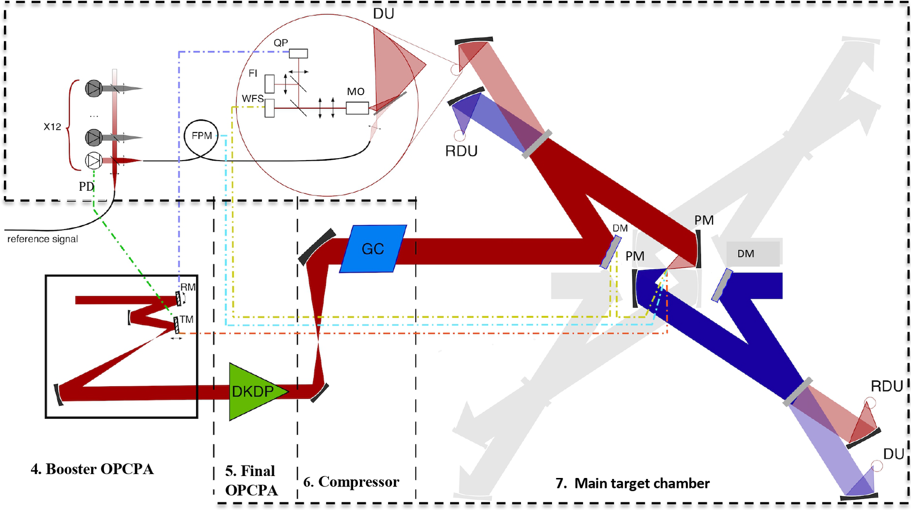
A DM with an appropriate aperture (55 cm × 55 cm or 66 cm × 66 cm, see Section 2.6) was made using a hybrid technology[ Reference Samarkin, Alexandrov, Galaktionov, Kudryashov, Nikitin, Rukosuev, Toporovsky and Sheldakova 88 ]. It is controlled by approximately 200 bimorph electrodes and 20 peripheral pushers based on stepper motors. The remote sensing algorithm requires several pulses, so the use of remote sensing for single ‘shots’ is inefficient. The DM operates with a low-power beam with a pulse repetition rate of 100 Hz. The wavefront is measured with a Hartmann sensor[ Reference Platt and Shack 89 , Reference Aleksandrov, Zavalova, Kudryashov, Rukosuev, Sheldakova, Samarkin and Romanov 90 ], and the quality of focusing is measured with a charge-coupled device (CCD) camera that records the energy distribution in the far-field. Two sets of sensors are used and, accordingly, two feedbacks, shown in Figure 14 by yellow lines. The main set (not shown in Figure 14) is moved into the main focus with the help of servos for the period of the auxiliary set calibration and then removed. The auxiliary set is located behind a flat mirror that directs the beam onto a parabolic mirror (Figure 14). First, the DM is tuned to the optimal surface shape, using data from the main set as feedback. Then the current values in the auxiliary set are recorded as reference values, after which the feedback of the adaptive system switches from the main set to the auxiliary one and maintains these reference values. Such a two-stage procedure is standard for high-power laser systems[ Reference Kotov, Perevalov, Starodubtsev, Zemskov, Alexandrov, Galaktionov, Kudryashov, Samarkin and Soloviev 91 ], including the PEARL laser, where a Strehl number of more than 0.72 was obtained with a beam diameter of 18 cm and a pulse energy of more than 10 J when focused by a parabolic mirror with a numerical aperture of F/2.5[ Reference Soloviev, Kotov, Martyanov, Perevalov, Zemskov, Starodubtsev, Alexandrov, Galaktionov, Samarkin, Kudryashov, Yakovlev, Ginzburg, Kochetkov, Shaikin, Kuzmin, Stukachev, Mironov, Shaykin and Khazanov 92 ].
Note that the focal waist can be shifted along the z-axis within a small range by DM-induced defocus, which is an alternative way to fine-tune the waist position. In some cases, this can help avoid moving large focusing mirrors and be useful for spatial overlapping of the focal waists of 12 beams separately.
For the procedure of spatial overlapping of beams in the main focus, auxiliary manipulations are required in each of the 12 channels, which include blocking, attenuation and reduction of the beam aperture. The corresponding devices (screen, filters, diaphragms) are inserted into the beam immediately after the splitter (see Section 2.4 and Figure 8). The direction of propagation of each beam is stabilized by means of a mirror rotating in two planes, controlled by a quad photodiode, located behind the flat mirror, which directs the beam onto the parabolic mirror. In Figure 14, this feedback is shown in violet. In addition, using CCD cameras, the energy distribution in the near-field of the beam is measured both before focusing and after it, behind the ‘foreign’ flat mirror, which directs the opposite beam to a parabolic mirror (retro-diagnostics) (Figure 14).
The method of spatial alignment of beams is based on the use of a thin blade[ Reference Soloviev, Burdonov, Chen, Eremeev, Korzhimanov, Pokrovskiy, Pikuz, Revet, Sladkov, Ginzburg, Khazanov, Kuzmin, Osmanov, Shaikin, Shaykin, Yakovlev, Pikuz, Starodubtsev and Fuchs 38 , Reference Kumar, Šmíd, Singh, Soloviev, Bohlin, Burdonov, Fente, Kotov, Lancia, Lédl, Makarov, Morrissey, Perevalov, Romanovsky, Pikuz, Kodama, Neely, McKenna, Laštovička, Starodubtsev, Weber, Nakatsutsumi and Fuchs 93 ], which makes it possible to match the edge of the blade with the focal waist ensuring subwavelength accuracy (Figure 15). The idea is based on the dependence of the near-field topology of the beam passing through the focus on the position of the blade relative to the focal plane. The blade located behind the waist (Figure 15(b)) blocks the beam from the blade insertion side. The blade located in front of the waist (Figure 15(c)) blocks the beam from the opposite side. Uniform fading out of brightness throughout the aperture indicates the position of the blade exactly in the focal plane (Figure 15(d)). The procedure allows for both moving the parabolic mirror to aim at the blade and placing the blade in the waist.
Illustration of blade alignment.

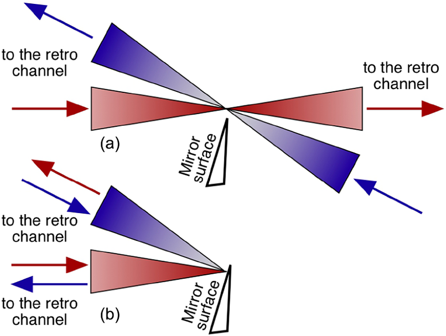
Spatial alignment of the 12 beams is carried out in two stages: overlapping of two counterpropagating beams and successive overlapping of adjoining beams. To match the opposite beams, the blade has a mirror surface, which is located along the normal to the beam, reflecting it back into the retro-diagnostic channel (Figure 16(b)). When the blade is removed from the waist, the counterpropagating beam enters the retro channel (Figure 16(a)). Thus, beam overlapping can be additionally diagnosed by comparing the position of the beam reflected from the blade and the beam of the counterpropagating channel. To overlap beams along two coordinates, it is necessary to use two blades rotated by 90°.
Overlapping of counterpropagating channels.

Similarly, the adjacent beams are overlapped, for which the blade is positioned in such a way that the reflected beam of one channel is directed exactly to the second channel (Figure 17). Unlike counterpropagating beams, this requires the use of two pairs of opposite channels at once. After the blade is placed in the focus of the first pair, the focus of the second pair is moved on the blade. Thus, the foci of all channels are combined at the single point, and then synchronization and phase-locking of the pulses are carried out.
Adjacent channels overlapping.
2.9 Synchronization and phase-locking of 12 pulses
After the focal waists of all 12 beams are made to coincide at one point in space, it is necessary to combine 12 pulses in time. The problem of making pulses coincident in time in a common focus can be divided into two parts: synchronization, that is, alignment of the pulse envelopes with an error much smaller than the pulse duration, and phase-locking, that is, alignment of the pulse phases in the focus with an error much smaller than the optical cycle. Note that carrier-envelope phase stabilization is not required, since the pulse duration is much longer than the optical cycle and 2 $\pi$
phase shift will not lead to a significant intensity decrease.
$\pi$
phase shift will not lead to a significant intensity decrease.
Ideal phase-locking (maximum intensity at the focus) is achieved when the phases of all pulses are exactly equal. Any random phase mismatch leads to an intensity decrease. For the usual (non-dipole) focusing geometry, a detailed analysis was carried out in Ref. [Reference Leshchenko94]. In particular, it is shown that for the standard deviation of phase $\pi /4$
, the intensity decreases by approximately 30%, while for
$\pi /4$
, the intensity decreases by approximately 30%, while for $\pi /2$
it decreases by 70%. We have carried out numerical simulations with dipole focusing. In this case, the intensity maximum was sought only in the equatorial plane. It can be seen from Figure 13 that for the dipole focusing, the effect of phase mismatch is less than for conventional focusing: the intensity decreases by 16% and 47%, respectively.
$\pi /2$
it decreases by 70%. We have carried out numerical simulations with dipole focusing. In this case, the intensity maximum was sought only in the equatorial plane. It can be seen from Figure 13 that for the dipole focusing, the effect of phase mismatch is less than for conventional focusing: the intensity decreases by 16% and 47%, respectively.
It is necessary not only to set the same path lengths, but also to dynamically compensate for fluctuations due to temperature drift, air currents and vibrations. To do this, a translator-driven mirror I is installed in each channel. The TM should have the smallest possible mass and, accordingly, aperture, so it is installed inside the telescope after the beam splitter (see also Figure 8). A feedback signal arrives at the TM. For synchronization, this feedback can be relatively slow (parts of a hertz) and, for phase-locking, the feedback bandwidth must reach tens of hertz. In single-pulse laser systems or systems with a low pulse repetition rate (less than 100 Hz), it is impossible to achieve such an operation rate; therefore, unamplified pulses are used for the feedback, which travel exactly the same path as amplified ones[ Reference Bagayev, Leshchenko, Trunov, Pestryakov and Frolov 95 ], since their repetition rate is much higher. According to Ref. [Reference Bagayev, Trunov, Pestryakov, Leschenko, Frolov and Vasiliev96], to compensate for fluctuations in a band up to 10 Hz, the pulse repetition rate must be at least 100 Hz. Feedback circuits can be based on the interference of signals with each other, including pairwise interference[ Reference Kienel, Müller, Klenke, Limpert and Tünnermann 97 ], or on joint focusing[ Reference Zhou, Liu, Wang, Ma, Ma, Xu and Guo 98 ], as well as on the interference of signals with one reference beam[ Reference Fsaifes, Daniault, Bellanger, Veinhard, Bourderionnet, Larat, Lallier, Durand, Brignon and Chanteloup 99 ]. In all cases, the error signals are generated, which are processed by the processor, then changing the voltage on the piezoelectric transducers, which shifts the TM mirrors in each channel.
The difference between the dipole focusing geometry and the usual geometry leads to two additional difficulties. Firstly, at the first stage of temporal alignment, the feedback signal is usually derived from the energy density in the focus, where a photodiode or a CCD camera is installed, but they cannot be used in a common focus of 12 beams, since they cannot be illuminated from all sides. Therefore, a special intensity sensor is required. It can be either a nanoscatterer whose image is transferred to a photodiode, a nanoantenna that receives a signal and transmits it to a detector[ Reference Yu and Zhan 100 ] or a nonlinear medium whose response is also monitored by a photodiode[ Reference Penjweini, Weber, Sondermann, Boyd and Leuchs 101 ]. An alternative would be pairwise convergence, but this seems to be more labor consuming and can take a long time. Secondly, at the second stage, when the sensor is removed from the focus, a replica of the focal waist is usually used instead, formed, for example by a beam that has passed through the nontransmitting mirror. However, such a replica cannot be created for all 12 beams upon dipole focusing. This problem is solved with the help of an additional feedback system based on the pulse phase measurement using a beam passing through the TM, a fiber-optic phase regulator and a mixer with a reference beam, followed by a photodiode (Figure 14).
Such a flexible architecture allows the use of various algorithms; we will dwell on two of them. In the first algorithm, the optimal positions of the TM are selected and maintained in such a way that the beams at the focus have zero phase shifts, that is, so that the maximum intensity is achieved on the sensor (red feedback loop in Figure 14). Next, the phase shift on each fiber-optic regulator is set so that the signal on the photodiode is maximum (blue feedback loop). At this time, the red feedback loop is turned on and maintains maximum intensity in the focus. Then the phases of the fiber-optic regulators are fixed (frozen), and the control of the positions of the TM is changed to maintain the maximum values of the signals on the photodiodes (green feedback loop). After that, the intensity sensor is no longer needed, and it is removed from the focus.
The second algorithm uses a green feedback loop from the very beginning: it selects and maintains the positions of the TM to lock the channels with each other. This guarantees a time-constant phase shift of the pulses in different channels, but does not guarantee its zero value. Then, using the fiber-optic controls on the sensor in focus, the maximum intensity is set (blue feedback loop). At this time, the green and blue feedback loops operate simultaneously. After reaching the maximum intensity, the voltages on the fiber-optic regulators are frozen (the blue feedback loop is broken), and the operation of the green loop ensures that the maximum intensity is maintained in the focus. The sensor is removed from the focus.
Note that both the direct beams that have passed through the TMs before the focus and the counter beams from retro-channels that have passed through the TMs after the focus can be directed to the photodiode. For more reliable and stable operation of the algorithm, both options can be used simultaneously.
2.10 Additional options: control of the pulse parameters after the compressor
As indicated in Section 2.6, the energy density of one XCELS channel is limited by the optical damage of diffraction gratings and, for a pulse duration of 20 fs, the intensity cannot be much higher than 10 TW/cm2. Recently, to further reduce the duration of petawatt and subpetawatt laser pulses, the post-compression method, also known as a TFC (thin film compressor)[
Reference Mourou, Mironov, Khazanov and Sergeev
32
] or the CafCA (compression after compressor approach)[
Reference Khazanov, Mironov and Mourou
34
] (Figure 18(a)), has become widely used. The essence of the method is to use a thin plane-parallel plate – a nonlinear element in which the spectrum of the laser pulse is significantly broadened due to self-phase modulation caused by the Kerr nonlinearity. Next, the phase of the spectrum $\varphi \left(\varOmega \right)$
is corrected with the help of chirped (dispersive) mirrors, which provides a pulse of shorter duration, close to a Fourier-transform-limited one. The method was confirmed in experiments, where a decrease in the duration of subpetawatt laser pulses by five[
Reference Ginzburg, Yakovlev, Zuev, Korobeynikova, Kochetkov, Kuzmin, Mironov, Shaykin, Shaikin, Khazanov and Mourou
102
] and six[
Reference Shaykin, Ginzburg, Yakovlev, Kochetkov, Kuzmin, Mironov, Shaikin, Stukachev, Lozhkarev, Prokhorov and Khazanov
103
] times was demonstrated. However, in these experiments and in most others[
Reference Khazanov
33
,
Reference Kim, Kim, Yang, Yoon, Sung, Lee and Nam
104
–
Reference Ginzburg, Yakovlev, Zuev, Korobeynikova, Kochetkov, Kuzmin, Mironov, Shaykin, Shaikin and Khazanov
106
], the intensity was of the order of 1 TW/cm2. At an intensity of 10 TW/cm2, submillimeter plates are required; therefore, it is promising to use polymer[
Reference Mironov, Gacheva, Ginzburg, Silin, Kochetkov, Mamaev, Shaykin, Khazanov and Mourou
107
,
Reference Masruri, Wheeler, Dancus, Fabbri, Nazîru, Secareanu, Ursescu, Cojocaru, Ungureanu, Farinella, Pittman, Mironov, Balascuta, Doria, Ros and Dabu
108
] or quartz[
109
] films placed at the Brewster angle. The simulation results for a quartz plate of 500 μm thick are shown in Figure 19 (green curves). The pulse is seen to be compressed to 2.6 fs, while the output pulse power increases by a factor of 4.6. In this case, the output power of one XCELS channel is 130 and 230 PW for two compressor options. The achievement of fivefold post-compression is also planned in Ref. [Reference Li, Kato and Kawanaka31] (see Table 1).
$\varphi \left(\varOmega \right)$
is corrected with the help of chirped (dispersive) mirrors, which provides a pulse of shorter duration, close to a Fourier-transform-limited one. The method was confirmed in experiments, where a decrease in the duration of subpetawatt laser pulses by five[
Reference Ginzburg, Yakovlev, Zuev, Korobeynikova, Kochetkov, Kuzmin, Mironov, Shaykin, Shaikin, Khazanov and Mourou
102
] and six[
Reference Shaykin, Ginzburg, Yakovlev, Kochetkov, Kuzmin, Mironov, Shaikin, Stukachev, Lozhkarev, Prokhorov and Khazanov
103
] times was demonstrated. However, in these experiments and in most others[
Reference Khazanov
33
,
Reference Kim, Kim, Yang, Yoon, Sung, Lee and Nam
104
–
Reference Ginzburg, Yakovlev, Zuev, Korobeynikova, Kochetkov, Kuzmin, Mironov, Shaykin, Shaikin and Khazanov
106
], the intensity was of the order of 1 TW/cm2. At an intensity of 10 TW/cm2, submillimeter plates are required; therefore, it is promising to use polymer[
Reference Mironov, Gacheva, Ginzburg, Silin, Kochetkov, Mamaev, Shaykin, Khazanov and Mourou
107
,
Reference Masruri, Wheeler, Dancus, Fabbri, Nazîru, Secareanu, Ursescu, Cojocaru, Ungureanu, Farinella, Pittman, Mironov, Balascuta, Doria, Ros and Dabu
108
] or quartz[
109
] films placed at the Brewster angle. The simulation results for a quartz plate of 500 μm thick are shown in Figure 19 (green curves). The pulse is seen to be compressed to 2.6 fs, while the output pulse power increases by a factor of 4.6. In this case, the output power of one XCELS channel is 130 and 230 PW for two compressor options. The achievement of fivefold post-compression is also planned in Ref. [Reference Li, Kato and Kawanaka31] (see Table 1).
Schemes of post-compression (a), post-compression with spectral filtering (b) and frequency doubling with post-compression (c). NE, nonlinear element; CM, chirped mirror; R( $\Omega$
) is a mirror whose reflection coefficient has a dip in the center of the spectral band; the dichroic mirrors shown in blue reflect the second harmonic of the pulse and transmit the first harmonic.
$\Omega$
) is a mirror whose reflection coefficient has a dip in the center of the spectral band; the dichroic mirrors shown in blue reflect the second harmonic of the pulse and transmit the first harmonic.

Spectra (a) and pulse intensity in linear (b) and logarithmic (c) scales at the grating compressor output (red curves), after post-compression (green curves) (see Figure 18(a)) and after post-compression with spectral filtering (blue curves) (see Figure 18(b)).

In addition to increasing the power, it is important to increase the pulse contrast, which is extremely important for many experiments, especially with solid-state and nanostructured targets. To this end, several options for upgrading the post-compression were proposed, of which the method of spectral filtering of the pulse after self-phase modulation[ Reference Buldt, Müller, Klas, Eidam, Limpert and Tünnermann 110 , Reference Mironov, Starodubtsev and Khazanov 111 ] is most suitable for the XCELS laser (see Figure 18(b)). The idea of the method is that, in contrast to the spectrum of the main pulse, the spectrum of the pedestal is not broadened, since its intensity is low. Consequently, if the band corresponding to the initial pulse is ‘cut out’ from the broadened spectrum, then the pedestal will be significantly reduced and the main pulse will suffer little, because its spectrum is much wider. For this, a mirror is used, the reflection coefficient of which has a dip in the center of the spectral band of the initial pulse. The choice of dip width is dictated by the compromise between increasing the temporal contrast and increasing the peak intensity of the compressed pulse. Figure 19 shows an example of calculation (blue curves): the intensity increased by a factor of 2.8 and the contrast increased by two orders of magnitude.
Technologically more complex, but even more attractive, are the generation and further compression of second harmonic pulses (Figure 18(c)). In this case, not only does the temporal contrast increase, but also, due to the shorter wavelength, the diameter of the focal spot is approximately halved, which significantly increases the intensity at the focus. The cubic nonlinearity affects the SHG both due to the broadening of the spectrum, which increases the dispersion spreading, and due to violation of the phase-matching conditions, since both the first harmonic pulse and the second harmonic pulse accumulate a time-dependent nonlinear phase. In the approximation of plane monochromatic waves, the latter effect can be completely compensated[ Reference Mironov, Lozhkarev, Ginzburg and Khazanov 112 ]. An intensity of the order of 10 TW/cm2 requires thin, wide-aperture nonlinear crystals, the fabrication of which is a complex technological problem. The most promising is the fabrication of a thin (~1 mm) silica substrate, which is glued with a transparent glue on a thick (~1 cm) KDP crystal, after which it is polished to the required thickness. Figure 20 shows the results of calculations for a crystal thickness of 250 μm and a silica substrate thickness of 1 mm. As expected, due to the quadratic nonlinearity, the contrast is squared, since in the calculations we assumed that the fundamental harmonic pulse is completely removed from the beam due to reflection from the spectrum splitters. In practice, the increase in contrast will be determined by the number and quality of the spectrum splitters. As can be seen from Figure 20, the pulse duration decreased to 3.4 fs and the peak power increased by a factor of 1.4, which, taking into account a twofold decrease in the wavelength, leads to an increase in the intensity at the focus by a factor of 5.6.
Pulses of the fundamental harmonic (red curves), the second harmonic (blue curves) and the second harmonic after post-compression (green curves).

Note that today the technological problem is the creation of broadband wide-aperture chirped mirrors with a high damage threshold. However, this problem may be solved in the future or alternative dispersion elements may be created (see, e.g., Ref. [Reference Mironov, Wheeler, Khazanov and Mourou113]). We also point out the potential possibility of self-compression of a focused pulse during its propagation in plasma[ Reference Kim, Litvak, Mironov and Skobelev 114 , Reference Pipahl, Anashkina, Toncian, Toncian, Skobelev, Bashinov, Gonoskov, Willi and Kim 115 ].
It is important to note that the application of the methods described in this section leads to wavefront distortions if the intensity distribution is not uniform over the cross-section. At present, methods have been proposed[ Reference Martyanov, Mironov, Starodubtsev, Soloviev, Kochetkov, Ginzburg, Shaykin and Khazanov 116 ] for determining the optimal corrective phase for restoring a flat front by the aid of an adaptive mirror; the results of the first successful experiments are reported in Ref. [Reference Soloviev, Kotov, Martyanov, Perevalov, Zemskov, Starodubtsev, Alexandrov, Galaktionov, Samarkin, Kudryashov, Yakovlev, Ginzburg, Kochetkov, Shaikin, Kuzmin, Stukachev, Mironov, Shaykin and Khazanov92]. Since the beams at the output of the XCELS laser channels are close to uniform, the wavefront distortions are much smaller than those indicated in Ref. [Reference Soloviev, Kotov, Martyanov, Perevalov, Zemskov, Starodubtsev, Alexandrov, Galaktionov, Samarkin, Kudryashov, Yakovlev, Ginzburg, Kochetkov, Shaikin, Kuzmin, Stukachev, Mironov, Shaykin and Khazanov92] and do not present any difficulties for the adaptive optics system described in Section 2.8.
To conclude Section 2, we present in Table 7 the power and focal intensity values that are expected to be obtained in the XCELS project. When planning the XCELS experimental program, it should be taken into account that these are the maximum values obtained for the maximum size of diffraction gratings (70 cm × 145 cm) and assuming a perfectly flat wave front. On the other hand, as mentioned above, the values presented in Table 7 are limited only by the dimensions and damage threshold of diffraction gratings, the manufacturing technologies of which are being actively developed. Gratings of 93 cm × 170 cm in size with the same robustness will allow compressing a beam with an aperture of 90 cm × 90 cm, which will increase the power of one channel to 100 PW. In this case, pumping the final OPCPA will require an energy of about 11 kJ, which is still less than 14 kJ, the energy of one channel of the UFL-2M facility[ Reference Garanin, Bel’kov and Bondarenko 60 , Reference Derkach, Derkach and Zhukov 61 ].
XCELS laser power and intensity.

3 eXawatt Center for Extreme Light Studies experimental program
Recently, possible experiments on multipetawatt laser systems have been actively discussed[ Reference Piazza, Willingale and Zuegel 117 ]. The XCELS project implies the creation of a unique laser system that makes it possible to generate optical pulses with record-breaking total power. Another important feature of the XCELS facility is its multichannel nature, which can be used to create complex distributions of light fields in the focus region, maximizing various pulse parameters, such as the laser field strength. Moreover, additional channels can be used both for diagnostic purposes and for generating intense fluxes of secondary radiation and particles, which may be needed in various experiments. Thus, a number of experiments are possible at the XCELS facility, which are inaccessible for other facilities, both existing and under construction. Possible experiments at the XCELS facility are the subject of special issues of the Kvantovaya Elektronika journal (English version: Bulletin of the Lebedev Physics Institute)[ Reference Berezin and Fedotov 118 – Reference Korzhimanov, Sladkov and Golubev 156 ], a review of which is given below.
It should be noted that laser technologies are developing very rapidly, which leaves a certain imprint on the XCELS project itself. At the first stage of the project, the power of the laser pulse in one channel was assumed to be approximately 15 PW, but, as mentioned above, recent progress in the technology of manufacturing diffraction gratings makes it possible to increase this power to 50 PW, and with the use of pulse post-compression even more. The proposals for the XCELS experimental program presented in Refs. [Reference Berezin and Fedotov118–Reference Korzhimanov, Sladkov and Golubev156] are mainly focused on the initial power (15 PW in one channel), but they remain relevant for several reasons. Firstly, these experiments can be carried out even before the XCELS facility reaches maximum power, which can take a very long time. Secondly, the operation of the facility with parameters significantly less than the maximum ones is more reliable and stable. Thirdly, some of the experiments can be directly ‘extrapolated’ for a higher power level, for example, by increasing the transverse size of the beam in the interaction region. Detailed theoretical studies of possible experiments on the XCELS facility for a maximum power level of 50 PW or more in one channel are expected to be carried out in the future.
Experiments can be provisionally divided into four groups: quantum electrodynamics (QED) processes in a strong laser field; generation and acceleration of particles; generation of secondary EM radiation; laboratory astrophysics, high energy density processes, diagnostics and other applications. The multichannel architecture of the XCELS setup is actively used in the experiments proposed in Refs. [Reference Berezin and Fedotov118–Reference Korzhimanov, Sladkov and Golubev156]. The numbers of laser pulses needed in the proposed experiments are shown in Figure 21. The proposed experiments are classified according to the studied phenomena. The blue color shows the minimum required number of laser pulses, while the cyan color shows the maximum number of pulses.
The number of laser pulses that are needed in the experimental schemes proposed in Refs. [Reference Berezin and Fedotov118–Reference Korzhimanov, Sladkov and Golubev156]. The blue color shows the minimum required number of laser pulses, while the cyan color shows the maximum number of pulses.

3.1 QED processes in a strong laser field
One of the most important goals of the XCELS project, which is of fundamental importance, is research in the field of the physics of strong EM fields, including the effects of high-field QED. Among such effects, we can single out vacuum polarization in a strong EM field, QED cascades, plasma dynamics with allowance for QED effects, etc.[ Reference Fedotov, Ilderton, Karbstein, King, Seipt and Torgrimsson 157 – Reference Marklund and Shukla 160 ]. Part of the experiments at the XCELS facility is related to the study of processes where high-field QED effects play a key role.
Thus, in Ref. [Reference Berezin and Fedotov118], a feasible experimental approach was proposed for studying vacuum polarization in a strong EM field using the XCELS facility. QED suggests that strong EM fields can affect vacuum quantum fluctuations. In this case, the vacuum behaves like a nonlinear medium and can be described by nonlinear radiative corrections to Maxwell’s equations. If the perturbation theory is applicable, then the main radiative corrections describe the four-wave interaction corresponding to elastic photon–photon scattering. In the case of a laser pulse of extremely high intensity, this allows observing interesting nonlinear optical phenomena, such as the generation of optical harmonics, self-focusing[ Reference Fedotov, Ilderton, Karbstein, King, Seipt and Torgrimsson 157 ]. Moreover, significant deviations of the coefficients measured in the experiment, which describe these nonlinear optical phenomena, from the calculated ones may indicate ‘new physics’. So far, such measurements have not been carried out, since they require extremely strong EM fields. At the same time, the XCELS facility fits perfectly for such experiments. In particular, a three-beam scheme for generating signal photons emitted by vacuum polarized by overlapping focused laser pulses with parameters corresponding to those of the XCELS setup was studied in Ref. [Reference Berezin and Fedotov118]. The authors in Ref. [Reference Berezin and Fedotov118] developed an efficient method for calculating the number and properties of signal photons. The dependence of the signal on the focusing and polarization of the pulses is analyzed and optimized, and the possibility of its detection in the XCELS multipetawatt facility is discussed and substantiated.
Another intriguing phenomenon predicted by high-field QED, which has not yet been observed in the laboratory, is the QED cascade[ Reference Nerush, Bashmakov and Kostyukov 161 – Reference Narozhnyi and Fedotov 166 ]. QED cascades can be conventionally considered as a process of converting light into matter. The mechanism of the QED cascade in a strong laser field is as follows. An electron, accelerated in a laser field, can emit a high-energy photon. Such a photon can decay in a strong field into an electron–positron pair. In turn, the resulting charged particles can also be accelerated and can emit hard photons. These two processes (emission of photons and their decay with the formation of electron–positron pairs) can be alternating for quite a long time, resembling a chain reaction. As a result, the number of secondary photons, electrons and positrons grows exponentially in time. In this case, laser pulse energy is converted into electron–positron plasma and hard EM radiation. It is generally believed that QED cascades are responsible for the generation of electron–positron plasma in the magnetosphere of neutron stars[ Reference Sturrock 167 ]. Also, EM showers caused by cosmic rays in the atmospheres of planets can be attributed to non-self-sustained QED cascades, where the energy of the cascade is extracted from the energy of cosmic rays[ Reference Gaisser 168 ]. To generate a QED cascade, a sufficiently strong EM field is required, which is not yet available under laboratory conditions. Such a field can be formed as a result of coherent combining of several XCELS laser pulses[ Reference Gonoskov, Aiello, Heugel and Leuchs 81 , Reference Gonoskov, Bashinov, Gonoskov, Harvey, Ilderton, Kim, Marklund, Mourou and Sergeev 169 ]. Depending on the pulse combining arrangement, the EM field in the focus region can be close to the field of an electric dipole wave (the electric field is maximum in focus) or a magnetic dipole wave (the magnetic field is maximum in focus).
Refs. [Reference Murav’ev, Bashinov, Efimenko, Panova, Volokitin, Meyerov, Kim and Sergeev119,Reference Bashinov, Efimenko, Murav’ev, Volokitin, Panova, Meyerov, Sergeev and Kim122] discuss experiments with a magnetic dipole wave generated by laser pulses from the XCELS facility. In Ref. [Reference Murav’ev, Bashinov, Efimenko, Panova, Volokitin, Meyerov, Kim and Sergeev119], the development of a QED cascade was studied using 3D numerical simulation by the particle-in-cell method and, in particular, the threshold total laser pulse power required for the cascade was determined. It was shown that the minimum breakdown threshold of 14 PW is achieved when using 12 beams; when the number of beams is reduced to 2–6, the threshold power increases and is set at the level of 18 PW. The dependence of the rate of development of a QED cascade on the number of laser beams was determined in a wide power range. It was demonstrated that fluctuations in the power of each of the beams have little effect on either the breakdown threshold or the rate of cascade development. In Ref. [Reference Bashinov, Efimenko, Murav’ev, Volokitin, Panova, Meyerov, Sergeev and Kim122], an experimental scheme was proposed for studying the radiative capture of electrons. So far, radiative capture has not been observed under laboratory conditions[ Reference Gonoskov, Gonoskov, Harvey, Ilderton, Kim, Marklund, Mourou and Sergeev 83 ]. The authors of Ref. [Reference Bashinov, Efimenko, Murav’ev, Volokitin, Panova, Meyerov, Sergeev and Kim122] showed that, when a nanowire solid target is irradiated by several petawatt laser pulses that maximize the magnetic field at the focus, an anomalous radiative capture regime can occur. The formed distributions of accelerated electrons and generated gamma photons have distinctive properties, based on which it is possible to experimentally determine the applicability of various theoretical approaches to the description of radiation losses. Configurations with different numbers of employed XCELS channels (4, 6 and 12) and with different total pulse power were considered.
The electric dipole configuration was discussed in Refs. [Reference Efimenko, Bashinov, Murav’ev, Panova, Volokitin, Meyerov, Kim and Sergeev120,Reference Efimenko, Bashinov, Murav’ev, Panova, Volokitin, Meyerov, Kim and Sergeev121], where the main attention was paid to the generation of gamma rays and charged particle fluxes from the region of the QED cascade. Using a full-scale numerical simulation, it was shown that when the parameters of the laser system are close to the declared parameters of the XCELS facility, the maximum energy of gamma ray photons can reach 2 GeV, the total efficiency of laser pulse energy conversion into photons is 40% and the flux of photons with energies above 1 GeV can approach 1025 photons/s. It was also demonstrated that when using 12 laser pulses with a duration of 30 fs, the total charge of accelerated electrons (positrons) can reach 250–270 nC, and the charge of particles with energies above 1 GeV can exceed 1 nC. The electric dipole structure of the fields makes it possible to obtain an extremely narrow (several milliradians) angular distribution of gamma photons and particles over the polar angle measured from the field symmetry axis. Thus, multibeam multipetawatt laser systems, such as XCELS, can become the basis for constructing a bright source of gamma radiation and positrons.
Coherent combining of laser pulses required for construction of a dipole wave at focus is a substantial technological challenge, especially for XCELS ultrahigh-power laser beams. Therefore, it is important to study theoretically and experimentally how the accuracy of pulse synchronization affects the development of QED cascades. This issue is discussed in Ref. [Reference Nerush, Iligenov and Kostyukov123], demonstrating the potential possibility of observing self-sustained QED cascades at the XCELS facility with a random phase difference of pulses in different channels for a total power of 36 PW. In this case, on average, the number of generated positrons can be an order of magnitude smaller than in the case of phased pulses collected in a dipole wave. However, with a probability of 10%–30%, a ‘shot’ of the XCELS facility with random phases will lead to the production of 1/4–1/3 of the number of positrons produced in the case of an electric dipole wave. The absorption of the laser field, which can also be a marker of the cascade development, is also significant and can reach up to 20% or more with a probability of 10%–30%. In Ref. [Reference Nerush, Iligenov and Kostyukov123], the power of the system, which significantly exceeds the threshold for the cascade development in an ‘in-phase’ configuration, was considered. Obviously, for near-threshold power, one can also expect the development of a cascade for random phases, but the probability of ‘successful’ shots can be significantly lower than in the considered case.
In the experiments with the dipole wave discussed above, in order to develop a QED cascade, it is necessary to place the seed particles in the region of a strong electric field. The way they should be placed requires further study. In this connection, it is interesting to analyze the possibility of the development of a QED cascade upon irradiation of various targets with laser pulses. In Ref. [Reference Samsonov, Kostyukov, Filipovic and Pukhov125], the development of a QED cascade and the formation of electron–positron pairs as a result of the interaction of the laser pulse with a foil are studied using full-size 3D numerical simulation by the particle-in-cell method. Consider two different interaction configurations. In the first configuration, six laser pulses are focused to one point on the target surface from the vertices of a regular hexagon. In the second configuration, laser pulses are focused in pairs to one point on the target surface from vertices located symmetrically with respect to the focusing point. In this case, the focus points for each pair are spaced the same distance from each other and lie on the same straight line. The polarization of the laser pulses is chosen so that the electric field lies in the plane formed by the normal to the target and the direction of the pulse propagation (tangential plane polarization). In both schemes, the normal to the target and the propagation direction of each laser pulse make an angle of 75°. It is shown that, with the laser pulse parameters foreseen at the XCELS facility, it is possible to generate electron–positron pairs with energies up to gigaelectronvolts, a total number of particles of 8×10¹⁰ and an average concentration of 2×1020 cm–3.
One of the effects that appears in a strong laser field is the back-reaction of radiation. The effect is due to the recoil that occurs when a photon is emitted. In a strong field, the electron is accelerated to a high energy, and the probability of emitting a photon that carries away a significant part of the electron’s energy increases greatly. In a simplified description, the radiation reaction effect can be represented as the effective radiative friction force (radiation reaction force) acting on the radiating particle. This effect can lead to interesting phenomena, such as radiative capture[
Reference Gonoskov, Gonoskov, Harvey, Ilderton, Kim, Marklund, Mourou and Sergeev
83
,
Reference Ji, Pukhov, Kostyukov, Shen and Akli
170
] and inverse Faraday effect[
Reference Kostyukov, Shvets, Fisch and Rax
171
,
Reference Liseykina, Popruzhenko and Macchi
172
]. Ref. [Reference Liseikina, Peganov and Popruzhenko124] is devoted to the possibility of observing the inverse Faraday effect at the XCELS facility. Since it is not easy to generate a circularly polarized pulse with high power, a configuration with two linearly polarized phased laser pulses propagating at a small angle to each other is considered. The presented calculation results show that the use of two 15-PW orthogonally polarized beams intersecting at a small angle (≤10 ${}^{\circ}$
) enables experimental observation of the inverse Faraday effect induced by radiative friction. The XCELS facility can generate a longitudinal quasi-static magnetic field with a peak intensity of several gigagauss.
${}^{\circ}$
) enables experimental observation of the inverse Faraday effect induced by radiative friction. The XCELS facility can generate a longitudinal quasi-static magnetic field with a peak intensity of several gigagauss.
3.2 Generation and acceleration of particles
The acceleration of charged particles is one of the processes that, on the one hand, is of great fundamental and applied importance and, on the other hand, can be experimentally studied at the XCELS facility. Due to the high intensity of laser pulse in the XCELS facility, one can expect particle fluxes with ultrahigh energy densities. The authors of Ref. [Reference Bychenkov and Lobok130] studied the generation of high-energy electron flows during the interaction of one pulse of the XCELS setup with a near-critical density target. Using numerical simulations, it is shown that in this case the charge of accelerated electrons with an energy of 0.2–2 GeV reaches about 0.1 μC. In this case, the efficiency of laser energy conversion into electron energy is 17%.
Laser–plasma methods of electron acceleration have recently attracted much attention due to the prospects of creating compact high-gradient accelerators[ Reference Esarey, Sprangle, Krall and Ting 173 , Reference Kostyukov and Pukhov 174 ]. It is assumed that the size of such accelerators will be several orders of magnitude smaller than the size of accelerators based on standard technologies. Impressive results have been obtained so far in this area. The energy of accelerated electrons has reached 8 GeV, which is comparable to the energy of particles in X-ray free electron lasers[ Reference Gonsalves, Nakamura, Daniels, Benedetti, Pieronek, de Raadt, Steinke, Bin, Bulanov, van Tilborg, Geddes, Schroeder, T'oth, Esarey, Swanson, Fan-Chiang, Bagdasarov, Bobrova, Gasilov, Korn, Sasorov and Leemans 175 ]. It should be noted that such energy was obtained at a length of several tens of centimeters, while the length of an accelerator for X-ray free electron lasers reaches hundreds of meters and kilometers. Even more energy can be obtained by taking advantage of the XCELS plant. It was shown in Ref. [Reference Dorozhkina, Baluev, Kutergin, Lotov, Minakov, Spitsyn, Tuev and Lotov131] by numerical simulation that an electron bunch with a charge of 50 pC can be accelerated to an energy of 100 GeV with a sub-percent energy spread using a single laser pulse from the XCELS setup. To do this, it is required to create a plasma channel 70 m long with a characteristic radius of 200 μm and a plasma density on the axis of 3 × 1015 cm–3. The initial laser pulse should be stretched to a duration of 200 fs, and its diameter should be about 400 μm.
Theoretically, even greater energy can be obtained using multistage acceleration, where at each stage the acceleration is carried out by its own laser pulse[ Reference Schroeder, Esarey, Geddes, Benedetti and Leemans 176 ]. Since the XCELS facility is multichannel, it is suitable for testing multistage acceleration schemes. The possibilities of experiments on multistage acceleration of electrons and positrons at the XCELS facility were studied in Refs. [Reference Starodubtseva, Tsymbalov, Ivanov, Gorlova and Savelyev132,Reference Veisman, Umarov, Pugacheva and Andreev135]. Using numerical simulations, it was shown in Ref. [Reference Veisman, Umarov, Pugacheva and Andreev135] that the facility can demonstrate the acceleration of an electron bunch in three to five stages to an energy of 60–100 GeV while maintaining its high quality (normalized emittance ~1 mm mrad, energy spread ~1%). The bunch charge was assumed to be 70 pC. Ref. [Reference Starodubtseva, Tsymbalov, Ivanov, Gorlova and Savelyev132] studied the multistage acceleration of electron bunches with a large charge. Calculations show the possibility of multistage acceleration of a bunch with a charge of 400 nC. A method for calculating a multistage accelerator is proposed taking into account the effects of dephasing and pump depletion; the method also allows estimating the parameters of the plasma channel for each acceleration stage and the admissible ranges for angles of electron injection into the next stage. In Ref. [Reference Kuznetsov, Umarova and Andreev136], a scheme for a laser–plasma injector was proposed. It is shown that with using such an injector it is possible to obtain bunches with an emittance of approximately 8 mm mrad, a charge of 100 pC and an energy of 150 MeV.
Of great interest are laser–plasma methods for generating and accelerating protons and ions[ Reference Macchi, Borghesi and Passoni 177 ]. Due to the high intensity of the laser pulse, protons can be accelerated in the radiation pressure regime. This regime has not yet been studied experimentally. The possibility of ion acceleration in the radiation pressure regime was studied in Ref. [Reference Samsonov and Kostyukov133] for the parameters of the XCELS facility using full-size 3D numerical simulation. The parameters of the laser pulse (degree of focusing) and the foil (electron density and thickness) are found to be optimal from the point of view of the efficiency of laser pulse energy conversion into ion energy, the cutoff energy of ions and the total charge of ions with an energy of more than 500 MeV/nucleon. It has been established that in the ‘laser drilling’ mode it is possible to obtain ions with a cutoff energy of approximately 750 MeV/nucleon and a charge of approximately 70 nC, and in the ‘light sail’ mode with a cutoff energy of approximately 1500 MeV/nucleon and a charge of approximately 50 nC. Numerical simulation shows that in both cases the conversion efficiency can exceed 30%.
It is known that low-density targets can provide more efficient interaction of the laser pulse with plasma. Ref. [Reference Brantov, Rakitina, Glazyrin and Bychenkov126] studied the generation of ions in the interaction of XCELS pulses with low-density targets. It is shown that the use of an expanding target with an optimal density profile being formed makes it possible to achieve a proton energy of the order of 1 GeV. Numerical calculations predict the conversion coefficients of the laser pulse energy into the energy of accelerated protons of up to 20% and the production of proton beams with an energy of more than 100 MeV at a total energy of more than 30 J. In Ref. [Reference Kovalev and Bychenkov128], the possibility of generating ions with energies reaching gigaelectronvolts using the Coulomb explosion is discussed. In this case, it is proposed to irradiate spherical microtargets with the XCELS laser pulse.
The laser pulse in the XCELS facility also makes it possible to generate neutrons, positrons and pions. In Ref. [Reference Gozhev, Bochkarev, Lobok, Brantov and Bychenkov127], recommendations were developed for obtaining a great number of laser-heated deuterons with moderate energies (0.2–2 MeV) at a level of 1015 per shot and for creating a bright source of thermonuclear DD neutrons with an expected peak flux of approximately 1018 particles cm–2 s–1. It was demonstrated in Ref. [Reference Lobok and Bychenkov129] that the use of an XCELS laser pulse would make it possible to achieve a record-high yield (1012) of MeV-energy positrons per shot. It was shown[ Reference Brantov, Lobok and Bychenkov 134 ] that the use of only one channel of the XCELS laser will make it possible to obtain a ultrahigh pion yield at the level of 108 particles per laser shot.
3.3 Generation of radiation in hard-to-reach regions of the EM spectrum
In these regions of the spectrum, the XCELS facility can provide record-breaking radiation for important applications[ Reference Consoli, Tikhonchuk, Bardon, Bradford, Carroll, Cikhardt, Cipriani, Clarke, Cowan, Danson and Angelis 178 ]. Refs. [Reference Vais, Lobok and Bychenkov137,Reference Lobok, Brantov and Bychenkov140,Reference Andreev, Umarov and Popov145] are devoted to the generation of EM radiation in the gamma range. In Ref. [Reference Andreev, Umarov and Popov145], a universal type of target based on low-density polymer aerogels was proposed, which can be used to create various sources of particles and quanta in the MeV energy range without changing the parameters of the XCELS laser facility. Simulation using the GEANT4 software package shows a high efficiency in the generation of gamma quanta and positrons with energies up to hundreds of megaelectronvolts. An increase in the number of laser pulses, focused on a low-density target, will lead to a proportional increase in the charge of electron and positron beams and the gamma ray flux to values unattainable by other methods.
In Ref. [Reference Vais, Lobok and Bychenkov137], the generation of gamma radiation based on the betatron mechanism is studied in self-trapping regime when the laser pulse corresponding to XCELS parameters propagates in a near-critical density target. It is shown that the proposed betatron radiation source has a high radiation directivity with an angular half-width of 150 mrad in the direction of laser pulse polarization and a wide spectrum with a critical frequency of about 10 MeV. Owing to the small size of the source, short generation time and narrow synchrotron radiation directivity, the brightness can reach values significantly exceeding 1023 photon s–1 mm–2 mrad–2 (at $\Delta \lambda /\lambda = 0.1\%$
).
$\Delta \lambda /\lambda = 0.1\%$
).
In addition to the betatron mechanism, hard EM radiation can be generated using a bremsstrahlung mechanism. It was demonstrated in Ref. [Reference Lobok, Brantov and Bychenkov140] that the XCELS laser system can be used to create a source of gamma radiation with a photon energy noticeably higher than 1 MeV at a total energy (~35 J), that is, with characteristics surpassing all those known for lasers of petawatt power level. This is achieved due to efficient acceleration of an electron beam from near-critical plasma in the relativistic self-trapping regime, which leads to the generation of electron beams with a charge of more than 0.1 μC and a maximum energy of more than 2 GeV. Such electron beams are capable of converting more than half of their energy into the energy of bremsstrahlung gamma radiation, for example, in a tantalum target converter. The possibility of using the proposed pulsed source of gamma radiation for deep radiography of dense objects with high spatial resolution is shown. This makes it possible to determine the shape of an object, even shielded with iron layers up to 0.4 m thick (corresponding to a linear density of 320 g/cm2), which is more than three times the screening thickness obtained to date.
Another range of the EM spectrum for which there are no ultrahigh-power sources is the terahertz (THz) range. This range is important for medical and biological applications, for materials science and solid-state physics, for the development of security systems, etc.[ Reference Liao and Li 179 , Reference Kampfrath, Tanaka and Nelson 180 ]. Laser–plasma methods can provide an alternative to traditional sources based on vacuum and semiconductor devices. Several methods for generating THz radiation at the XCELS facility have been proposed[ Reference Kuratov, Brantov and Bychenkov 138 , Reference Kuratov, Brantov, Kovalev and Bychenkov 139 , Reference Volchok, Annenkov, Berendeev and Timofeev 141 – Reference Gorlova, Tsymbalov, Ivanov and Savelyev 143 ]. The authors of Ref. [Reference Kuratov, Brantov, Kovalev and Bychenkov139] studied the mechanism of transition radiation for the generation of terahertz unipolar pulses. Experimental implementation of generating THz pulses at the XCELS facility will make it possible to obtain unique unipolar pulses with an ultrahigh energy of approximately 1–5 J and a power of approximately 10–50 TW in the frequency range up to 2 THz, which is still unattainable using traditional methods. A decrease in the size of the focusing spot and an increase in the intensity of the laser pulse on the target lead to an increase in the characteristic cutoff frequency of the spectrum to approximately 6 THz, with virtually no change in the power and energy of the generated THz pulse.
In Ref. [Reference Gorlova, Tsymbalov, Ivanov and Savelyev143], using numerical simulations, two schemes of interaction of a 15-PW laser pulse with a target were considered: a one-stage scheme with one film target, in which electrons are accelerated and THz radiation is generated, and a two-stage scheme, where in the first target a beam of accelerated electrons is created, which then generates THz radiation passing through the second film target. Frequency-angular emission spectra in the THz range were obtained for these cases. The simulation results show that the THz field strength reaches a relativistic magnitude.
The generation of high-power directional radiation in the THz range by discharge currents excited by irradiation of an extended target of a given geometry by multipetawatt laser pulses was considered in Ref. [Reference Bukharsky, Kulikov and Korneev142]. It is shown that the use of several laser pulses makes it possible to proportionally increase the intensity of the emitted THz pulses and achieve a conversion efficiency of the order of several percent. The amplitude of the magnetic field obtained in the simulation at the boundaries of the computational grid, located at a distance of 0.64 mm from the radiation source, is about 400 T. The development of targets that, on the one hand, will be elements of a radiation source, and, on the other hand, will be able to collimate and transport the energy of THz radiation, is the subject of Ref. [Reference Kuratov, Brantov and Bychenkov138], where the THz pulse generation during the XCELS laser beam interaction with a cylindrical metal target was simulated numerically. It is shown that THz radiation is generated in a unique form, as a unipolar pulse, and a microwire target allows concentrating a significant part of the radiation near its surface and transporting it also in the form of a unipolar pulse at a speed close to the speed of light along the wire over long distances with low attenuation. The use of all planned 12 channels of the XCELS facility will make it possible to increase the charge of the escaping electrons by an order of magnitude and thereby significantly increase the amplitude and total energy of the generated near-surface EM pulses.
Another method for generating THz radiation was proposed in Ref. [Reference Volchok, Annenkov, Berendeev and Timofeev141]. In this paper, the authors consider a new method for generating high-power narrow-band THz radiation in the process of nonlinear interaction of counterpropagating laser wake waves, whose potential profiles are modulated in the transverse direction and locally do not coincide with each other. Each of the plasma waves with such a small-scale transverse structure is proposed to be created by a pair of interfering laser pulses propagating at a small angle to each other. Numerical simulation by the particle-in-cell method confirms the possibility of obtaining a narrow spectral line (2%) and a high efficiency of energy conversion at a level of 1% in such a scheme. With the design parameters of the XCELS facility, the proposed method opens the way to achieving terawatt pulse power in the THz frequency range.
Recently, sources of high-power radiation in the mid-infrared (mid-IR) range have attracted great interest[ Reference Pullen, Wolter, Le, Baudisch, Hemmer, Senftleben, Schröter, Ullrich, Moshammer, Lin and Bieger 181 ]. Such sources are in demand, for example, in spectroscopy. In Ref. [Reference Mikheytsev and Korzhimanov144], the possibility of generating extremely intense pulses in the mid-IR range during the interaction of XCELS laser pulses with matter is analyzed. The generation mechanism is based on the Doppler effect, which occurs when a laser pulse is reflected from a near-critical density plasma. It is shown that the highest efficiency (of the order of tenths of a percent) is observed at the shortest possible duration of the incident laser pulse and when it is sharply focused into a spot with a diameter of less than 2 μm. The use of two pulses allows increasing the efficiency by 1.5–2 times. Thus, it is possible to generate pulses in the wavelength range above 3 μm with an energy of several joules.
3.4 Laboratory astrophysics, processes with high energy density, diagnostics and other applications
Another area of application of laser plasma, which has been actively developed in recent years, is laboratory astrophysics[ Reference Bulanov, Esirkepov, Habs, Pegoraro and Tajima 182 ]. Since direct experiments in this area are in most cases impossible in the foreseeable future, much attention is paid to experiments whose results can be approximately extrapolated to real astrophysical phenomena using similarity methods. Ref. [Reference Bukharsky and Korneev147] demonstrated the possibility of using one or several femtosecond laser pulses of the XCELS facility to create a strong quasi-stationary magnetic field frozen in a relativistic supercritical density plasma. Due to the optimal conditions for laser–plasma interaction, a high efficiency of laser energy conversion into magnetic field energy is achieved – up to 20% according to the above calculations – and the magnetic induction is about 105 T. The resulting system with relativistic magnetized electrons and magnetic fields up to several tens of kilotesla is of interest for laboratory studies of high-energy processes in astrophysics, in particular, the phenomenon of relativistic reconnection of magnetic field lines. Ref. [Reference Sladkov and Korzhimanov151] is also devoted to experiments on magnetic reconnection. It is shown that when two laser pulses with a duration of 250–1000 fs are focused normally into spots with a diameter of 2–4 μm separated by 10–50 μm onto a solid target a few micrometers thick, two bunches of magnetized expanding plasma with a magnetization parameter of approximately 5 are formed on the back side of the target. Upon collision of these bunches, the conditions for magnetic reconnection are observed. Another direction of experimental research related to laboratory astrophysics is the achievement of ultrahigh pressures, which can also be obtained using a high-power laser pulse. It was shown[ Reference Korzhimanov, Sladkov and Golubev 156 ] that for the parameters of laser pulses that are planned to be obtained at the XCELS facility it is possible to produce matter with pressure values of more than 1 Gbar at a solid-state density, which corresponds to an energy release at the level of tens of MJ/g.
Let us dwell on the generation of superstrong quasi-stationary magnetic and electric fields. Ref. [Reference Dmitriev and Korneev150] considers two methods for generating strong magnetic fields with laser pulses corresponding to the XCELS setup, based on the use of structured targets and structured pulses. It is shown that the axial magnetic fields can reach tens of kilotesla in structured microcapillary targets. In the case of structured laser pulses interacting with a homogeneous plasma, an axial magnetic field of about tens of tesla can occupy a region about hundreds of micrometers in diameter. Ref. [Reference Serebryakov and Kostyukov153] studied the generation of an ultrastrong electric field in a solid target with a spherical cavity irradiated by laser pulses. Configurations of two, four and eight laser pulses are considered. The formation of a quasi-static strong electric field at the center of the cavity as a result of target collapse is demonstrated. Estimates show that for the parameters of the XCELS facility in an eight-beam configuration, a maximum electric field amplitude of 1.61 × 10¹⁴ V/cm can be expected. The possibility of creating hot plasma objects with the laser pulses from the XCELS facility, in which reactions of fusion of light nuclei take place, is discussed in Ref. [Reference Guskov and Korneev148]. For this purpose, it is proposed to use microsized targets in which superstrong magnetic or electric quasi-stationary fields are generated. It is assumed that magnetic fields will suppress electronic thermal conductivity and contribute to the confinement of charged products of nuclear reactions, while electric fields will lead to implosive compression of matter.
The XCELS laser system makes it possible to form several beams of probing and/or exciting gamma radiation at once, as well as fluxes of other particles (electrons, protons, neutrons, etc.). Such beams can be formed with a controlled time delay. This opens up unique prospects for research, including metastable and unstable isotopes and their isomers[ Reference Nedorezov, Rykovanov and Savel’ev 183 ]. It was shown in Ref. [Reference Shulyapov, Zavorotny and Savelyev152] that when a solid-state Kr target is irradiated, approximately 103 states with an energy of 9.4 keV can be excited in just one laser pulse. Their lifetime is 156.8 ns; however, the subnanosecond duration of the gamma ray pulse makes it possible to register the decay of these states. The possibility of accumulating nuclei at a level with an energy of 41.6 keV and the formation of a population inversion at the transition between levels with an energy difference of 9.4 keV is also discussed.
The XCELS laser system provides unique opportunities for research in the field of atomic physics and nonlinear optics. One of the interesting processes in a superstrong EM field is the so-called collective field ionization of an atom, when electrons do not leave the atom sequentially, that is, several atomic electrons can leave the atom at the same time. In a relativistically strong EM field, this process has been little studied so far. Ref. [Reference Popruzhenko and Tyurin154] reports the probability estimates for simultaneous tunneling of two electrons from multiply charged Li-like ions in a high-intensity laser field. Since very high intensities are required to observe the effect, the proposed scheme of the experiment to search for the collective tunneling effect requires laser pulses of extreme power, which are planned to be obtained at the XCELS facility. Another interesting effect related to ionization is relativistic electron tunneling through the Coulomb barrier. The possibility of observing both the relativistic tunneling effect during the ionization of multiply charged ions of heavy atoms in the field of multipetawatt laser beams and the deviation of the ionization rate from the values predicted by the nonrelativistic theory is discussed in Ref. [Reference Popruzhenko155].
Diagnostics of the processes that occur during the interaction of multipetawatt laser beams with matter is still a serious challenge for experimental physics. This is due both to the small space–time region where these processes occur, and to the high strengths of the EM fields that exist in the interaction region. The latter circumstance makes traditional diagnostic methods inapplicable. Therefore, the development of methods for diagnosing extreme light is currently of primary importance. Ref. [Reference Vays, Ivanov, Tsymbalov, Bukharsky, Bychenkov, Korneev and Savelyev-Trofimov146] proposes an approach to measure the key parameters of the XCELS beam, such as its size and peak intensity in the caustic. The proposed method is based on the use of vacuum acceleration of charged particles, electrons and protons, from the focal volume. In addition, it is assumed that the use of modern methods of machine learning will make it possible to restore the parameters of the laser pulse with ultrahigh intensity from the accumulated statistics of experimental data. Ref. [Reference Ryazantsev, Pikuz and Korneev149] discusses the features of X-ray spectral diagnostics in an ultrarelativistic laser plasma, taking into account the high temperature, high density and high magnetic fields in the plasma. Such a plasma, in particular, is formed when microstructured targets are irradiated with a multipetawatt laser pulse.
4 Conclusion
One channel of the XCELS laser system is potentially capable of providing an intensity at the focus several times higher than 1024 W/cm2. Post-compression of the pulse will make it possible to overcome the level of 1025 W/cm2. Dipole focusing of pulses from 12 channels, even without post-compression and without phasing, will bring the intensity closer to 1026 W/cm2. In the case of channel phasing, the intensity will be several times higher. The unique capabilities of the XCELS setup in the field of experimental physics of superstrong EM fields are associated not only with these record-breaking intensity values, but also with multibeam architecture. The latter makes it possible to carry out experiments with complex distributions of laser fields and with additional channels of laser and secondary radiation, which may be important for diagnosing processes in the field of interaction.
Acknowledgement
The work was supported by the Ministry of Science and Higher Education of the Russian Federation (Project No. 0030-2021-0015).


 Open access