


1. Introduction
Determining the growth of large-scale structures in disordered or turbulent systems that are initially homogeneous is a long-standing and challenging problem in many areas of fluid dynamics. To analyse the development of such structures, one typically seeks evolution equations whose coefficients depend on average properties of the underlying homogeneous flows. An obvious first question concerns the form of such coefficients and their dependence on the symmetries of the problem. A second question, which is much less often addressed in detail, but is nonetheless of great importance, is whether the formal expressions that arise can actually be calculated in a meaningful way.
To address these two questions by means of a concrete example, in this paper we consider the long-wavelength instabilities of a homogeneous nonlinear magnetohydrodynamical (MHD) state. Our treatment thereby extends the simpler kinematic studies of, on the one hand, the classical theory of mean field electrodynamics (see Krause & Rädler Reference Krause and Rädler1980; Moffatt & Dormy Reference Moffatt and Dormy2019) and, on the other, the so-called anisotropic kinetic alpha (AKA) hydrodynamic instability introduced by Frisch, She & Sulem (Reference Frisch, She and Sulem1987). Kinematic theory has undoubtedly been of enormous importance in the development of the subject. Nonetheless, in reality, the velocity is not prescribed but is driven by body forces, which, crucially, include the back-reaction of the magnetic field on the flow (the Lorentz force); this may be termed the dynamic theory. Furthermore, dynamo action in highly electrically conducting fluids, such as those that pertain astrophysically, typically results in fields that are of similar or smaller spatial scale to the flow – a small-scale dynamo (see e.g. Childress & Gilbert Reference Childress and Gilbert1995). These considerations naturally lead to the analysis of the problem of the growth of a large-scale magnetic field (and flow) from a basic MHD state, such as may result from the saturation of a small-scale dynamo. Crucially, in contrast to the kinematic case, the velocity and magnetic field now have equal prominence. By analogy with the kinematic problem, the aim is to derive coupled equations for the linear instability of the small-scale MHD basic state to large-scale perturbations of the magnetic and velocity fields; the tensorial coefficients are again determined from the basic state. Since this basic state can be highly nonlinear and chaotic, calculation of the coefficients may be far from straightforward. Nonetheless, a knowledge of the form of these tensors is very useful in understanding the role of symmetry and chirality in determining the growth of the instability. In § 2 we revisit the formal development of the equations, first expounded in Courvoisier, Hughes & Proctor (Reference Courvoisier, Hughes and Proctor2010a), and provide new explicit expressions for the coefficients in a particular case. Simplified versions of this problem have been considered by Courvoisier et al. (Reference Courvoisier, Hughes and Proctor2010a) and Courvoisier, Hughes & Proctor (Reference Courvoisier, Hughes and Proctor2010b). Courvoisier et al. (Reference Courvoisier, Hughes and Proctor2010a) studied large-scale instabilities of two-dimensional MHD flows, thereby extending the seminal work of Roberts (Reference Roberts1970, Reference Roberts1972) from the kinematic to the dynamic regime. Courvoisier et al. (Reference Courvoisier, Hughes and Proctor2010b) considered the full three-dimensional problem, but in order to obtain explicit expressions for the tensorial coefficients, it was assumed that both the fluid and magnetic Reynolds numbers were small, with magnetic fields generated through imposed small-scale electric currents. We also note that there have been other related studies with the aim of extracting mean field coefficients using perturbation schemes (see e.g. Yoshizawa Reference Yoshizawa1990; Yokoi Reference Yokoi2023; Schrinner et al. Reference Schrinner, Rädler, Schmitt, Rheinhardt and Christensen2005). We discuss how the various approaches differ in § 2.
For a given MHD turbulence configuration, in order to apply the theory expounded in § 2, it is necessary to calculate the linear response of the turbulence to the imposition of kinematic uniform (mean) flows and uniform magnetic fields; the tensorial coefficients are defined in terms of spatial and temporal averages of quadratic fluctuating quantities. There are parallels between this method and classical linear response theory, which is used to address small perturbations to Hamiltonian systems (see Kubo Reference Kubo1966; Marconi et al. Reference Marconi, Puglisi, Rondoni and Vulpiani2008).
In § 3, we calculate the tensorial coefficients, after linearising the perturbation equations, for a variety of basic state configurations. Reassuringly, we show through specific examples that there are circumstances in which this approach works perfectly, with convergence to well-defined mean quantities. We then use these coefficients to determine the nature of any long-wavelength instabilities of the flows and fields in question. We demonstrate that the instabilities arising from the traditional  $\alpha$ and AKA effects should not be considered in isolation. There are, however, circumstances in which the perturbed quantities, and hence quadratic averages of these, increase exponentially in time, and the theory, as formulated, simply cannot be applied. This divergence forms the basis of what is known as van Kampen's objection to classical linear response theory (Van Kampen Reference Van Kampen1971; Marconi et al. Reference Marconi, Puglisi, Rondoni and Vulpiani2008). It does, however, prompt the interesting question of whether the theory can be rescued by considering the fully nonlinear problem with arbitrary imposed fields and flows – for which the average quantities will be well-defined (see e.g. Proctor Reference Proctor2022) – and then considering the weak field/flow (kinematic) limit of this dynamical approach. What will be the nature of the response in this kinematic limit? In particular, is it guaranteed to be linear? These are questions that may be posed in a somewhat wider context. If a nonlinear dynamical system – not necessarily hydrodynamical – is perturbed, is the response of the system readily measurable and, if so, is the response linear in the magnitude of the perturbation?
Such questions go beyond the realm of linear response theory and are best addressed by a combination of analysis and numerical computation. In order to gain some elementary understanding, before tackling the full horrors of the MHD turbulence problem in § 5, in § 4 we explore this issue by considering the ostensibly simpler problem of calculating the responses to small symmetry-breaking terms of a variety of one-dimensional maps. The nature of the response turns out to depend crucially on the form of the invariant measure of the system.
In § 5, we expand on the dichotomy outlined in § 4 by reverting to the full nonlinear MHD problem and attempting to calculate the tensorial coefficients in the limit of weak imposed fields and flows. As has been noted in other studies of MHD turbulence, the signal-to-noise ratio can be extremely small, thereby creating difficulties with obtaining well-defined averages. Furthermore, even when averages can be obtained, a linear response is more detectable for some mean field tensors than for others.
A summary of our results is contained in § 6; we also discuss the inherent difficulties in extracting the signal (i.e. the response) from the noise (i.e. the turbulent fluctuations), a problem that seems particularly marked in MHD turbulence. In addition, we assess to what extent one may carry over the results from the one-dimensional maps discussed in § 4 to the infinite-dimensional MHD equations.
2. Mathematical and computational formulation
2.1. The long-wavelength stability problem
The basic state of our problem comprises statistically steady and homogeneous incompressible MHD turbulence, driven by a prescribed forcing  $\boldsymbol {F}(\boldsymbol {x},t)$. It is supposed that the velocity field $\boldsymbol {U}$ and the magnetic field $\boldsymbol {B}$ are periodic in a cuboidal domain with typical size $L$. After a standard non-dimensionalisation, the momentum and induction equations take the form
 $$\begin{gather}
\frac{\partial \boldsymbol{U}}{\partial t}
+\boldsymbol{U}\boldsymbol{\cdot }\boldsymbol{\nabla}\boldsymbol{U}
={-}\boldsymbol{\nabla} P + \boldsymbol{B}
\boldsymbol{\cdot }\boldsymbol{\nabla}\boldsymbol{B} +
Re^{{-}1} \nabla^2 \boldsymbol{U} +\boldsymbol{F},
\end{gather}$$
$$\begin{gather}
\frac{\partial \boldsymbol{U}}{\partial t}
+\boldsymbol{U}\boldsymbol{\cdot }\boldsymbol{\nabla}\boldsymbol{U}
={-}\boldsymbol{\nabla} P + \boldsymbol{B}
\boldsymbol{\cdot }\boldsymbol{\nabla}\boldsymbol{B} +
Re^{{-}1} \nabla^2 \boldsymbol{U} +\boldsymbol{F},
\end{gather}$$ $$\begin{gather}\frac{\partial
\boldsymbol{B}}{\partial t}
+\boldsymbol{U}\boldsymbol{\cdot }\boldsymbol{\nabla}\boldsymbol{B}
= \boldsymbol{B}\boldsymbol{\cdot }
\boldsymbol{\nabla}\boldsymbol{U} + Rm^{{-}1} \nabla^2
\boldsymbol{B} .
\end{gather}$$
$$\begin{gather}\frac{\partial
\boldsymbol{B}}{\partial t}
+\boldsymbol{U}\boldsymbol{\cdot }\boldsymbol{\nabla}\boldsymbol{B}
= \boldsymbol{B}\boldsymbol{\cdot }
\boldsymbol{\nabla}\boldsymbol{U} + Rm^{{-}1} \nabla^2
\boldsymbol{B} .
\end{gather}$$
The Reynolds number  $Re$ and the magnetic Reynolds number $Rm$ are defined as usual by $Re=\hat {U}L/\nu$ and $Rm=\hat {U}L/\eta$, where $\hat {U}$ is a typical velocity, $\nu$ is the kinematic viscosity and $\eta$ is the magnetic diffusivity. Here we prescribe the forcing and not the velocity, and so $\hat {U}^2/L=\hat {F}$, where $\hat {F}$ is a typical magnitude of the forcing. We are interested in finding the growth rate of very long-wavelength disturbances to this basic state. We assume that these disturbances are small, so that the perturbation equations can be linearised. We start by writing down the linearised equations for the perturbation quantities, denoted by $\boldsymbol {u}$, $p$ and $\boldsymbol {b}$:
 $$\begin{gather} \frac{\partial \boldsymbol{u}}{\partial t} +\boldsymbol{U}\boldsymbol{\cdot }\boldsymbol{\nabla}\boldsymbol{u} +\boldsymbol{u}\boldsymbol{\cdot }\boldsymbol{\nabla}\boldsymbol{U} ={-}\boldsymbol{\nabla} p + \boldsymbol{B}\boldsymbol{\cdot }\boldsymbol{\nabla}\boldsymbol{b} + \boldsymbol{b}\boldsymbol{\cdot }\boldsymbol{\nabla}\boldsymbol{B}+ Re^{{-}1} \nabla^2 \boldsymbol{u}, \end{gather}$$
 $$\begin{gather}\frac{\partial \boldsymbol{b}}{\partial t} +\boldsymbol{U}\boldsymbol{\cdot }\boldsymbol{\nabla}\boldsymbol{b} +\boldsymbol{u}\boldsymbol{\cdot }\boldsymbol{\nabla}\boldsymbol{B} = \boldsymbol{B}\boldsymbol{\cdot }\boldsymbol{\nabla}\boldsymbol{u} +\boldsymbol{b}\boldsymbol{\cdot }\boldsymbol{\nabla}\boldsymbol{U} + Rm^{{-}1} \nabla^2 \boldsymbol{b} . \end{gather}$$
We now assume that these quantities evolve on two disparate length and time scales. By averaging over intermediate scales, we can therefore write  $\boldsymbol {u}=\bar {\boldsymbol {u}}+\boldsymbol {u}'$, etc., where the barred (mean) variables vary only on length and time scales, denoted by $\boldsymbol {X}$ and $T$, respectively, that are very long compared with the scales $\boldsymbol {x}$ and $t$ of the basic state. Equations (2.3) and (2.4) may then be decomposed into mean and fluctuating parts. The mean equations take the form
 $$\begin{gather} \frac{\partial \bar{\boldsymbol{u}}}{\partial T} +\frac{\partial}{\partial X_j}(\overline{U_j \boldsymbol{u}'} + \overline{u'_j \boldsymbol{U}}) ={-}\boldsymbol{\nabla}_{\!\!{\tiny X}} \bar{p} +\frac{\partial}{\partial X_j}(\overline{B_j \boldsymbol{b}'} + \overline{b'_j \boldsymbol{B}})+ Re^{{-}1} {\nabla}_{\!\!{\tiny X}}^2 \bar{\boldsymbol{u}}, \end{gather}$$
 $$\begin{gather}\frac{\partial \bar{\boldsymbol{b}}}{\partial T} = \boldsymbol{\nabla}_{\!\!{\tiny X}}\times( \overline{\boldsymbol{U}\times\boldsymbol{b}'} + \overline{\boldsymbol{u}'\times\boldsymbol{B}}) + Rm^{{-}1} {\nabla}_{\!\!{\tiny X}}^2 \bar{\boldsymbol{b}} , \end{gather}$$
where  $(\boldsymbol {\nabla }_{\!\!{\tiny X}})_i=\partial /\partial X_i$. To close these equations we need to express the averaged quantities in terms of $\bar {\boldsymbol {u}}$ and $\bar {\boldsymbol {b}}$. If we wish only to find terms including first derivatives of $\bar {\boldsymbol {u}}$ and $\bar {\boldsymbol {b}}$ with respect to $\boldsymbol {X}$ (since these terms will dominate at sufficiently long scales), we can self-consistently neglect derivatives of $\bar {\boldsymbol {u}}$, $\bar {\boldsymbol {b}}$ in the equations for the fluctuations. With this approximation, these then take the form
 \begin{align}
\frac{\partial \boldsymbol{u}'}{\partial t} +(\boldsymbol{U}\boldsymbol{\cdot }\boldsymbol{\nabla}\boldsymbol{u}'
+\boldsymbol{u}'\boldsymbol{\cdot }\boldsymbol{\nabla}\boldsymbol{U})'
+\bar{\boldsymbol{u}}\boldsymbol{\cdot }\boldsymbol{\nabla}\boldsymbol{U} &={-}\boldsymbol{\nabla}
p'+(\boldsymbol{B}\boldsymbol{\cdot }\boldsymbol{\nabla}\boldsymbol{b}'+\boldsymbol{b}'
\boldsymbol{\cdot }\boldsymbol{\nabla}\boldsymbol{B})'\nonumber\\
&\quad
+\bar{\boldsymbol{b}}\boldsymbol{\cdot }\boldsymbol{\nabla}\boldsymbol{B}+
Re^{{-}1} \nabla^2 \boldsymbol{u}',
\end{align}
\begin{align}
\frac{\partial \boldsymbol{u}'}{\partial t} +(\boldsymbol{U}\boldsymbol{\cdot }\boldsymbol{\nabla}\boldsymbol{u}'
+\boldsymbol{u}'\boldsymbol{\cdot }\boldsymbol{\nabla}\boldsymbol{U})'
+\bar{\boldsymbol{u}}\boldsymbol{\cdot }\boldsymbol{\nabla}\boldsymbol{U} &={-}\boldsymbol{\nabla}
p'+(\boldsymbol{B}\boldsymbol{\cdot }\boldsymbol{\nabla}\boldsymbol{b}'+\boldsymbol{b}'
\boldsymbol{\cdot }\boldsymbol{\nabla}\boldsymbol{B})'\nonumber\\
&\quad
+\bar{\boldsymbol{b}}\boldsymbol{\cdot }\boldsymbol{\nabla}\boldsymbol{B}+
Re^{{-}1} \nabla^2 \boldsymbol{u}',
\end{align}
 \begin{align} \frac{\partial
\boldsymbol{b}'}{\partial t} + ( \boldsymbol{U}
\boldsymbol{\cdot } \boldsymbol{\nabla} \boldsymbol{b}' +
\boldsymbol{u}' \boldsymbol{\cdot } \boldsymbol{\nabla}
\boldsymbol{B} )' +
\bar{\boldsymbol{u}}\boldsymbol{\cdot }\boldsymbol{\nabla}
\boldsymbol{B} &= ( \boldsymbol{B}
\boldsymbol{\cdot } \boldsymbol{\nabla} \boldsymbol{u}' +
\boldsymbol{b}' \boldsymbol{\cdot }
\boldsymbol{\nabla}\boldsymbol{U} )' \nonumber\\
&\quad + \bar{\boldsymbol{b}}
\boldsymbol{\cdot }\boldsymbol{\nabla} \boldsymbol{U} +
Rm^{{-}1} \nabla^2 \boldsymbol{b}' .
\end{align}
\begin{align} \frac{\partial
\boldsymbol{b}'}{\partial t} + ( \boldsymbol{U}
\boldsymbol{\cdot } \boldsymbol{\nabla} \boldsymbol{b}' +
\boldsymbol{u}' \boldsymbol{\cdot } \boldsymbol{\nabla}
\boldsymbol{B} )' +
\bar{\boldsymbol{u}}\boldsymbol{\cdot }\boldsymbol{\nabla}
\boldsymbol{B} &= ( \boldsymbol{B}
\boldsymbol{\cdot } \boldsymbol{\nabla} \boldsymbol{u}' +
\boldsymbol{b}' \boldsymbol{\cdot }
\boldsymbol{\nabla}\boldsymbol{U} )' \nonumber\\
&\quad + \bar{\boldsymbol{b}}
\boldsymbol{\cdot }\boldsymbol{\nabla} \boldsymbol{U} +
Rm^{{-}1} \nabla^2 \boldsymbol{b}' .
\end{align}
It can be seen that each of  $\boldsymbol {u}'$ and $\boldsymbol {b}'$ is subject to forcing from both $\bar {\boldsymbol {u}}$ and $\bar {\boldsymbol {b}}$. It is assumed that the long-time solutions of (2.7) and (2.8) are (statistically) unique, consistent with the basic state being a (statistical) attractor. If (2.7) and (2.8) are formally solved, and the results substituted into (2.5) and (2.6), then we obtain at leading order, after dropping the diffusive terms, which are subdominant at small wavenumbers:
 $$\begin{gather} \frac{\partial \bar{u}_i}{\partial T} +\frac{\partial}{\partial X_j}(\varGamma^{(1)}_{ijl}\bar{u}_l+\varGamma^{(2)}_{ijl}\bar{b}_l) ={-}\frac{\partial\bar{p}}{\partial X_i} , \end{gather}$$
 $$\begin{gather}\frac{\partial \bar{{b}}_i}{\partial T} = \epsilon_{ijk}\frac{\partial}{\partial X_j}( \alpha^{(1)}_{kl} \bar{{b}}_l +\alpha^{(2)}_{kl}\bar{u}_l ) . \end{gather}$$
The quantities  $\boldsymbol {\varGamma }^{(i)}$, $\boldsymbol {\alpha }^{(i)}$ are tensors, depending only on the properties of the basic state $\boldsymbol {U}$, $\boldsymbol {B}$ and so ultimately on those of $\boldsymbol {F}$ (to be more precise, $\boldsymbol {\varGamma }^{(1)}$ and $\boldsymbol {\alpha }^{(2)}$ are true tensors, whereas $\boldsymbol {\varGamma }^{(2)}$ and $\boldsymbol {\alpha }^{(1)}$ are pseudo-tensors). The $\boldsymbol {\varGamma }^{(i)}$ are always symmetric in their first two indices, whereas the $\boldsymbol {\alpha }^{(i)}$ have no symmetries in general. It is important to note that since we are considering forced turbulence in a fixed frame of reference, our system is not Galilean invariant; in a Galilean-invariant system, the tensors $\boldsymbol {\varGamma }^{(1)}$ and $\boldsymbol {\alpha }^{(2)}$ would vanish.
Two of the mean quantities appearing in (2.9) and (2.10) are familiar:  $\boldsymbol {\alpha }^{(1)}$ is the well-known dynamo $\alpha$-effect, which has been extensively discussed in the literature; $\boldsymbol {\varGamma }^{(1)}$ can be recognised as the AKA effect introduced by Frisch et al. (Reference Frisch, She and Sulem1987). The other terms, which couple the two mean field equations, and were first introduced by Courvoisier et al. (Reference Courvoisier, Hughes and Proctor2010a), have not been widely studied. It is interesting to note that reflectionally symmetric turbulence leads to constraints on $\boldsymbol {\alpha }^{(1)}$ and $\boldsymbol {\varGamma }^{(2)}$, being pseudo-tensors (e.g. the symmetric part of $\boldsymbol {\alpha }^{(1)}$ vanishes), whereas there are no such constraints on $\boldsymbol {\alpha }^{(2)}$ and $\boldsymbol {\varGamma }^{(1)}$.
As noted in the introduction, it is of interest to compare our formulation with other approaches to obtaining mean field tensors in turbulent MHD. Yoshizawa (Reference Yoshizawa1990) (see also Yokoi Reference Yokoi2023) considered a two-scale approach to MHD turbulence, adopting the two-scale direct-interaction approximation (TSDIA), retaining the effects both of the mean quantities and their derivatives, thus capturing effects such as eddy diffusivities, which we do not consider here. Yoshizawa (Reference Yoshizawa1990) considered a system that was Galilean invariant and, as such, the tensors  $\boldsymbol {\varGamma }^{(1)}$ and $\boldsymbol {\alpha }^{(2)}$ vanish. Moreover, under the TSDIA, $\boldsymbol {\varGamma }^{(2)}$ also vanishes. Schrinner et al. (Reference Schrinner, Rädler, Schmitt, Rheinhardt and Christensen2005) adopted a very different approach. They extracted the fluctuating velocity from a stationary MHD turbulent state – possibly one with a mean magnetic field – and then solved the fluctuating induction equation after the imposition of so-called ‘test fields’, which may be functions of position. They then calculated the resulting electromotive force (e.m.f.), which they related to the $\alpha _{ij}$ and $\beta _{ijk}$ tensors of mean field MHD. Although their starting point is a saturated MHD state, they did not consider the equation for the mean velocity.
2.2. Determining the tensors  ${\alpha}^{(i)}$ and ${\varGamma}^{(i)}$ under the ‘short-sudden’ approximation


Obtaining analytic expressions for the mean quantities  $\bar {\boldsymbol {u}}$, $\bar {\boldsymbol {b}}$ is not, in general, possible. However, there are two special cases in which progress can be made. One is when both $Re$ and $Rm$ are small, which has already been considered in Rädler & Brandenburg (Reference Rädler and Brandenburg2010) and Courvoisier et al. (Reference Courvoisier, Hughes and Proctor2010b). The other, which we consider here, is when the correlation time of the turbulence is short and one may adopt the ‘short-sudden’ approximation (see e.g. Krause & Rädler Reference Krause and Rädler1980). In this case, (2.7) and (2.8) are approximated at leading order by
 \begin{equation} \boldsymbol{u}'=\tau_1(\bar{\boldsymbol{b}}\boldsymbol{\cdot }\boldsymbol{\nabla}\boldsymbol{B}-\bar{\boldsymbol{u}}\boldsymbol{\cdot }\boldsymbol{\nabla}\boldsymbol{U}),\quad \boldsymbol{b}'=\tau_2(\bar{\boldsymbol{b}}\boldsymbol{\cdot }\boldsymbol{\nabla}\boldsymbol{U}-\bar{\boldsymbol{u}}\boldsymbol{\cdot }\boldsymbol{\nabla}\boldsymbol{B}), \end{equation}
where  $\tau _1$ and $\tau _2$ are, respectively, the correlation times for the fluctuating flow and field. Note that $\boldsymbol {u}'$ is automatically solenoidal, and so the pressure gradient does not enter this approximation. Substituting for $\boldsymbol {u}'$ and $\boldsymbol {b}'$ into (2.5) and (2.6) allows us to calculate the mean field tensors. It is straightforward to show that $\boldsymbol {\varGamma }^{(1)}$ vanishes in this special case, since
 \begin{align}
\varGamma_{ijl}^{(1)} &={-}\tau_1 \left( \overline{U_j
\frac{\partial U_i}{\partial x_l}} +
\overline{\frac{\partial U_j}{\partial x_l} U_i }\right) +
\tau_2 \left( \overline{B_j \frac{\partial B_i}{\partial
x_l}} + \overline{\frac{\partial B_j}{\partial x_l} B_i
}\right)
\end{align}
\begin{align}
\varGamma_{ijl}^{(1)} &={-}\tau_1 \left( \overline{U_j
\frac{\partial U_i}{\partial x_l}} +
\overline{\frac{\partial U_j}{\partial x_l} U_i }\right) +
\tau_2 \left( \overline{B_j \frac{\partial B_i}{\partial
x_l}} + \overline{\frac{\partial B_j}{\partial x_l} B_i
}\right)
\end{align} \begin{align} &={-}\tau_1 \overline{\frac{\partial \left(U_i U_j \right)}{\partial x_l}} + \tau_2 \overline{\frac{\partial \left( B_i B_j \right)} {\partial x_l}} =0. \end{align}
The elements of the tensors  $\boldsymbol {\alpha }^{(1)}$, $\boldsymbol {\alpha }^{(2)}$ and $\boldsymbol {\varGamma }^{(2)}$ are given by
 $$\begin{gather} \alpha_{il}^{(1)} = \epsilon_{ipq} \left( \tau_2\overline{U_p \frac{\partial U_q}{\partial x_l}} - \tau_1 \overline{B_p \frac{\partial B_q}{\partial x_l}} \right), \end{gather}$$
 $$\begin{gather}\alpha^{(2)}_{il}=(\tau_1-\tau_2)\epsilon_{ipq}\gamma_{pql}, \end{gather}$$
 $$\begin{gather}\varGamma^{(2)}_{ijl}= (\tau_2+\tau_1)(\gamma_{ijl}+\gamma_{jil}), \end{gather}$$
where
 \begin{equation} \gamma_{ijl} = \overline{U_i\frac{\partial B_j}{\partial x_l}} ={-} \overline{B_j\frac{\partial U_i}{\partial x_l}} = \frac{1}{2} \left( \overline{U_i\frac{\partial B_j}{\partial x_l}} - \overline{B_j\frac{\partial U_i}{\partial x_l}} \right). \end{equation}
It should be noted that under the short-sudden approximation, the equations for the fluctuating flow and field, (2.11a,b), take a simplified form. As a consequence,  $\boldsymbol {\alpha }^{(1)}$ contains only products of $\boldsymbol {U}$ with itself and $\boldsymbol {B}$ with itself – in general, however, there is no reason to expect that $\boldsymbol {\alpha }^{(1)}$ will not contain products of $\boldsymbol {U}$ and $\boldsymbol {B}$. In a similar vein, when $\tau _1=\tau _2$, the symmetry of (2.11a,b) leads to the vanishing of the $\boldsymbol {\alpha }^{(2)}$ tensor, although $\tau _1$ and $\tau _2$ cannot be calculated a priori in general. There is an analogous situation in the approximated system introduced by Rädler & Brandenburg (Reference Rädler and Brandenburg2010), in which $\boldsymbol {\alpha }^{(2)}$ vanishes when $Re=Rm$.
The expression for  $\boldsymbol {\alpha }^{(1)}$, which first appeared in Pouquet, Frisch & Léorat (Reference Pouquet, Frisch and Léorat1976), is the extension of the classical $\alpha$-effect from hydrodynamic to magnetohydrodynamic basic states; the velocity and magnetic fields are clearly on an equal footing, as indicated in the introduction. It is worth noting that this form of $\boldsymbol {\alpha }^{(1)}$ is sometimes interpreted as a ‘quenching’ mechanism for the $\alpha$-effect as a dynamo evolves to finite amplitude; there are, however, problems with such an interpretation, as noted by Proctor (Reference Proctor2003). The two terms that couple the basic state velocity and magnetic fields ( $\boldsymbol {\alpha }^{(2)}$ and $\boldsymbol {\varGamma }^{(2)}$) rely for their existence on different parts of $\gamma _{ijl}$. In particular, since $\boldsymbol {\varGamma }^{(2)}$ is symmetric in its first two arguments, it will vanish if the statistics of the basic state are isotropic. The coefficients of the $\gamma _{ijl}$ tensor are a priori almost unconstrained, although since $\boldsymbol {U}$ and $\boldsymbol {B}$ are solenoidal, we do have $\gamma _{iji} = \gamma _{ijj} = 0$. It is straightforward to show that for isotropic turbulence, $\alpha ^{(2)}_{il} = \tilde \alpha \delta _{il}$, where
 \begin{equation} \tilde{\alpha}={-}\left( \frac{\tau_1-\tau_2}{3} \right) \overline{\boldsymbol{U} \boldsymbol{\cdot } \boldsymbol{\nabla} \times \boldsymbol{B}} ={-}\left( \frac{\tau_1-\tau_2}{3} \right) \overline{\boldsymbol{B} \boldsymbol{\cdot } \boldsymbol{\nabla} \times \boldsymbol{U}}. \end{equation}
It is of interest to note that even if the traditional  $\alpha$-effect ( $\boldsymbol {\alpha }^{(1)}$) vanishes, it still seems that there can be a long-wavelength instability induced by the coupling terms. Seeking solutions proportional, for example, to $\exp ({\rm i}(KZ + \omega T))$, so that $\bar {u}_3=\bar {{b}}_3=0$, we have the coupled two-dimensional algebraic equations (where $G^{(1)}_{ij}=\gamma _{i3j}$, $G^{(2)}_{ij}=\gamma _{3ij}$),
 \begin{equation} \omega \bar{\boldsymbol{u}}={-}(\tau_1+\tau_2) K({\boldsymbol{G}^{(1)}+ \boldsymbol{G}^{(2)})}\bar{\boldsymbol{b}}, \quad \omega \bar{\boldsymbol{b}}= (\tau_1 - \tau_2) K({\boldsymbol{G}^{(1)}- \boldsymbol{G}^{(2)}})\bar{\boldsymbol{u}},\end{equation}
and so  $\omega ^2$ is an eigenvalue of the matrix
 \begin{equation} (\tau_2^2 -\tau_1^2)K^2 ({\boldsymbol{G}^{(1)}+\boldsymbol{G}^{(2)}})({\boldsymbol{G}^{(1)}-\boldsymbol{G}^{(2)}}). \end{equation}
Unless both eigenvalues  $\omega ^2$ are real and positive, the basic state will be unstable. It therefore appears that there is a new generic mechanism for long-wavelength instability, relying on coupling between the mean momentum and induction equations and on anisotropy in the basic flow statistics.
2.3. From formalism to calculation
In theory, numerical calculation of the  $\boldsymbol {\varGamma }^{(i)}$ and $\boldsymbol {\alpha }^{(i)}$ tensors in (2.9) and (2.10) is straightforward, albeit computationally expensive. Following the standard mean field prescription, the fluctuating fields $\boldsymbol {u}'$ and $\boldsymbol {b}'$ are calculated from the linear equations (2.7) and (2.8), solved in concert with the nonlinear equations (2.1) and (2.2), following the imposition of uniform mean velocity and magnetic fields, $\bar {\boldsymbol {u}}$ and $\bar {\boldsymbol {b}}$. From the fluctuating fields, we construct the linearised mean total stress and the linearised mean e.m.f., defined by
 $$\begin{gather} R_{ij} = \overline{(U_j u_i'} + \overline{u'_j U_i)} - \overline{(B_j b_i'} + \overline{b'_j B_i)}, \end{gather}$$
 $$\begin{gather}{\boldsymbol{\mathcal{E}}} = \overline{\boldsymbol{U}\times\boldsymbol{b}'} + \overline{\boldsymbol{u}'\times\boldsymbol{B}}. \end{gather}$$
Varying the directions of  $\bar {\boldsymbol {u}}$ and $\bar {\boldsymbol {b}}$ allows calculation of all the tensorial coefficients, after spatial and temporal averaging of the various quadratic interactions, with the proviso that the requisite averages exist.
By contrast, when the averages do not exist, it is necessary, as discussed in the introduction, to consider fully nonlinear responses to the imposition of mean fields and flows. We restore the nonlinear terms into the perturbation equations (cf. (2.3) and (2.4)), which now take the form
 $$\begin{gather} \frac{\partial \boldsymbol{u}}{\partial t} +\boldsymbol{U}\boldsymbol{\cdot }\boldsymbol{\nabla}\boldsymbol{u} +\boldsymbol{u}\boldsymbol{\cdot }\boldsymbol{\nabla}\boldsymbol{U} +\boldsymbol{u}\boldsymbol{\cdot }\boldsymbol{\nabla}\boldsymbol{u} ={-}\boldsymbol{\nabla} p + \boldsymbol{B}\boldsymbol{\cdot }\boldsymbol{\nabla}\boldsymbol{b} + \boldsymbol{b}\boldsymbol{\cdot }\boldsymbol{\nabla}\boldsymbol{B} + \boldsymbol{b}\boldsymbol{\cdot }\boldsymbol{\nabla}\boldsymbol{b} + Re^{{-}1} \nabla^2 \boldsymbol{u}, \end{gather}$$
 $$\begin{gather}\frac{\partial \boldsymbol{b}}{\partial t} +\boldsymbol{U}\boldsymbol{\cdot }\boldsymbol{\nabla}\boldsymbol{b} +\boldsymbol{u}\boldsymbol{\cdot }\boldsymbol{\nabla}\boldsymbol{B} +\boldsymbol{u}\boldsymbol{\cdot }\boldsymbol{\nabla}\boldsymbol{b} = \boldsymbol{B}\boldsymbol{\cdot }\boldsymbol{\nabla}\boldsymbol{u} +\boldsymbol{b}\boldsymbol{\cdot } \boldsymbol{\nabla}\boldsymbol{U} + \boldsymbol{b}\boldsymbol{\cdot }\boldsymbol{\nabla}\boldsymbol{u} + Rm^{{-}1} \nabla^2 \boldsymbol{b} , \end{gather}$$
where, again,  $\boldsymbol {u}=\bar {\boldsymbol {u}}+\boldsymbol {u}'$, etc. Equations (2.23) and (2.24) are solved in concert with (2.1) and (2.2). The mean total stress and the mean e.m.f. now take the form
 $$\begin{gather} R_{ij} = \overline{(U_j u_i'} + \overline{u'_j U_i} + \overline{u_i' u_j')} - \overline{(B_j b_i'} + \overline{b'_j B_i} + \overline{b_i' b_j')}, \end{gather}$$
 $$\begin{gather}{\boldsymbol{\mathcal{E}}} = \overline{\boldsymbol{U}\times\boldsymbol{b}'} + \overline{\boldsymbol{u}'\times\boldsymbol{B}} + \overline{\boldsymbol{u}' \times \boldsymbol{b}'}. \end{gather}$$
 The MHD equations are solved on a cubic,  $2{\rm \pi}$-periodic domain, using a parallelised, dealiased, pseudospectral code. Time advancement of the diffusive terms is carried out exactly using an integrating factor, and the remaining terms are treated using a third-order Runge–Kutta scheme. For a detailed description of the numerical method, see Cattaneo, Emonet & Weiss (Reference Cattaneo, Emonet and Weiss2003). The simulations with the largest Reynolds numbers have a spatial resolution of $128^3$ grid points. Very long time evolutions are required in order to obtain meaningful averages; a single simulation can consume on the order of $10^4$ core hours. A series of simulations with different orientations and strengths of the mean fields is required in order to measure $\boldsymbol {\alpha }^{(i)}$ and $\boldsymbol {\varGamma }^{(i)}$.
3. Symmetry breaking in nonlinear MHD (i): linearised perturbations
In this section, we describe the results of direct numerical simulations to calculate the coefficients of the  $\boldsymbol {\varGamma }^{(i)}$ and $\boldsymbol {\alpha }^{(i)}$ tensors in the mean field equations (2.9) and (2.10). We have considered a variety of forcing functions $\boldsymbol {F}$ that, at low values of $Re$ and with no magnetic field, lead to spatially simple flows of the kind often used in kinematic dynamo studies. Of course our basic state here, governed by (2.1) and (2.2), will be more complicated even at low $Re$, as it involves the saturation through the Lorentz force of a small-scale dynamo. At high values of $Re$ and $Rm$, all simplicity is lost and the basic state, even under a simple forcing, is disordered both spatially and temporally. Here we concentrate on two particular forms of the forcing, defined by
 \begin{equation} \boldsymbol{F} = \boldsymbol{F}_1 = \frac{1}{Re}( \sin z + \cos y, \sin x + \cos z, \sin y + \cos x) \end{equation}
and
 \begin{align}
\boldsymbol{F} = \boldsymbol{F}_2 &= 2 \sin2t (\sin y,
-\sin x , \cos x + \cos y) \nonumber\\ &\quad +\frac{2}{Re}
(\sin y \sin ^2 t, \sin x \cos^2 t, \cos y \sin^2 t- \cos x
\cos^2 t) + \frac{\boldsymbol{F}_1}{2}.
\end{align}
\begin{align}
\boldsymbol{F} = \boldsymbol{F}_2 &= 2 \sin2t (\sin y,
-\sin x , \cos x + \cos y) \nonumber\\ &\quad +\frac{2}{Re}
(\sin y \sin ^2 t, \sin x \cos^2 t, \cos y \sin^2 t- \cos x
\cos^2 t) + \frac{\boldsymbol{F}_1}{2}.
\end{align}
In the absence of magnetic field, and at sufficiently small  $Re$, the forcing $\boldsymbol {F}_1$ drives the well-known $1{:}1{:}1$ ABC flow, $\boldsymbol {U}= Re \boldsymbol {F}_1$; since this flow is maximally helical (i.e. velocity parallel to vorticity), then the nonlinear terms can be balanced by a pressure gradient. This flow has a long and distinguished history in dynamo theory, dating back to the pioneering work of Childress (Reference Childress1970), Arnold & Korkina (Reference Arnold and Korkina1983) and Galloway & Frisch (Reference Galloway and Frisch1984). We are interested in cases where $Rm$ is sufficiently large that the ABC flow acts as a small-scale dynamo. The basic state then results from the equilibration of the dynamo instability, and indeed any hydrodynamic instability, resulting in a flow for which $\boldsymbol {B}$ is non-zero and $\boldsymbol {U}$ differs from the target flow.
As discussed below, the flows resulting from forcing  $\boldsymbol {F}_1$ possess symmetries that lead to the ‘cross-term tensors’ $\boldsymbol {\varGamma }^{(2)}$ and $\boldsymbol {\alpha }^{(2)}$ being zero. In order to discover a basic state that yields non-zero $\boldsymbol {\varGamma }^{(2)}$ and $\boldsymbol {\alpha }^{(2)}$ tensors, we investigated a variety of less symmetric forcings. The forcing $\boldsymbol {F}_2$ is the sum of $\boldsymbol{F}_1/2$ and that which drives the so-called MW $+$ flow of Otani (Reference Otani1993) at low $Re$.
$Re$.
3.1. When the linear theory works well
In this subsection, we investigate long-wavelength instabilities to the basic state generated by forcings  $\boldsymbol {F}_1$ and $\boldsymbol {F}_2$ at low values of $Re$ and fairly low values of $Rm$ (though high enough to support dynamo action, so that the basic states are magnetohydrodynamic).
First we consider forcing  $\boldsymbol {F}_1$, with $Re=Rm=12$; the basic MHD state for these particular parameters has been studied in some detail by Galanti, Sulem & Pouquet (Reference Galanti, Sulem and Pouquet1992). In the absence of magnetic field, the 1:1:1 ABC flow is hydrodynamically stable; it does though support dynamo action for $Rm=12$, and so an initially weak field is amplified until a stationary MHD state is attained in which the flow varies from its hydrodynamic state. For these parameter values, the basic MHD state has regular periodic oscillations, with mean values of $\langle U^2 \rangle \approx 1.67$ and $\langle B^2 \rangle \approx 0.057$, where $\langle {\cdot } \rangle$ denotes a volume and time average. This new state is not isotropic, but has a preferred direction, which depends on initial conditions; this state corresponds to the long-time solution shown in figure 3 of Galanti et al. (Reference Galanti, Sulem and Pouquet1992). Representative two-dimensional slices of the flow and field of the basic MHD state are shown in figure 1; here the preferred direction is along the $x$-axis. Interestingly, although the flow differs from its kinematic (hydrodynamic) form, it is, nonetheless, almost maximally helical, i.e. with $\langle\boldsymbol {U} \boldsymbol{\cdot } \boldsymbol {\nabla } \times \boldsymbol {U}\rangle/\sqrt {\langle U^2 \rangle \langle |\boldsymbol {\nabla } \times \boldsymbol {U}|^2 \rangle } \approx 1$.
Snapshots of representative slices of the basic state flow and field for forcing  $\boldsymbol {F}_1$, with $Re=Rm=12$. From left to right: (a,b,c) $U_x(y,z)$, $U_y(x,z)$, $U_z(x,y)$; (d,e,f) $B_x(y,z)$, $B_y(x,z)$, $B_z(x,y)$.

The flow is perturbed, in turn, by the imposition of kinematic uniform fields and flows in the  $x$,
$x$,  $y$ and $z$ directions, allowing us to calculate $R_{ij}$ and ${\boldsymbol{\mathcal{E}}}$ given by (2.21) and (2.22). By imposing magnetic fields, we can determine $\boldsymbol {\alpha }^{(1)}$ and $\boldsymbol {\varGamma }^{(2)}$, whereas from the imposed flows we can determine $\boldsymbol {\alpha }^{(2)}$ and $\boldsymbol {\varGamma }^{(1)}$. Here, the linear perturbations are also periodic in time and hence the quadratic quantities needed to calculate the mean field tensors must have well-defined averages. When the mean values are non-zero, convergence to the mean is rapid; however, for certain cases where the mean value is zero, some components of the Reynolds stress converge in amplitude faster than others. After imposing mean magnetic fields, the tensor $\boldsymbol {\alpha }^{(1)}$ is calculated as
 \begin{equation}
\boldsymbol{\alpha}^{(1)} = \left( \begin{array}{@{}c@{\quad}c@{\quad}c@{}} -1.22
& 0 & 0 \\ 0 & -0.043 & 0 \\ 0 & 0 & -0.043 \end{array}
\right),
\end{equation}
\begin{equation}
\boldsymbol{\alpha}^{(1)} = \left( \begin{array}{@{}c@{\quad}c@{\quad}c@{}} -1.22
& 0 & 0 \\ 0 & -0.043 & 0 \\ 0 & 0 & -0.043 \end{array}
\right),
\end{equation}
where the symmetries of the tensor indicate that the basic state for this run is isotropic in the  $yz$-plane. The symmetries of the flow and field are such that all components of the tensor $\boldsymbol {\varGamma }^{(2)}$ are zero. On imposing a mean flow, all components of the tensor $\boldsymbol {\alpha }^{(2)}$ are similarly zero; the only non-zero components of $\boldsymbol {\varGamma }^{(1)}$ are given by
 \begin{equation} \varGamma^{(1)}_{132} = \varGamma^{(1)}_{312} ={-}\varGamma^{(1)}_{123} ={-}\varGamma^{(1)}_{213} =0.058. \end{equation}
 Since both the tensors  $\boldsymbol {\alpha }^{(2)}$ and $\boldsymbol {\varGamma }^{(2)}$ are zero, as a consequence of the symmetries of the basic state, the mean field equations (2.9) and (2.10) are decoupled. Any instability that results is therefore either purely magnetic or purely hydrodynamic, although the basic flow of course depends crucially on both the flow and field.
To obtain insight into the magnetic instability, we consider a scaled form of  $\boldsymbol {\alpha }^{(1)}$ given by (3.3), namely
 \begin{equation}
\boldsymbol{\alpha}^{(1)} = \left( \begin{array}{@{}c@{\quad}c@{\quad}c@{}} -1 &
0 & 0 \\ 0 & -\varepsilon & 0 \\ 0 & 0 & -\varepsilon
\end{array} \right).
\end{equation}
\begin{equation}
\boldsymbol{\alpha}^{(1)} = \left( \begin{array}{@{}c@{\quad}c@{\quad}c@{}} -1 &
0 & 0 \\ 0 & -\varepsilon & 0 \\ 0 & 0 & -\varepsilon
\end{array} \right).
\end{equation}
On seeking solutions of the form  $\exp ({\rm i} \boldsymbol {K} \boldsymbol{\cdot } \boldsymbol {X} + S T)$, (2.10) leads to the following expression for the growth rate $S$:
$S$:
 \begin{equation} S ={\pm} \left( \varepsilon K_H^2 + \varepsilon^2 K_X^2 \right)^{1/2}, \end{equation}
where  $K_H^2 = K_Y^2 + K_Z^2$. The next order correction to (3.6) is $O(|\boldsymbol {K}|^2)$ and comprises molecular diffusion together with eddy effects that would result from inclusion of the first derivatives of $\bar {\boldsymbol {u}}$ and $\bar {\boldsymbol {b}}$ in the above analysis. For illustrative purposes, if we just retain the molecular terms, the extension of (3.6) becomes
 \begin{equation} S ={\pm} \left( \varepsilon K_H^2 + \varepsilon^2 K_X^2 \right)^{1/2} - Rm^{{-}1} \left( K_H^2 + K_X^2\right). \end{equation}
For  $\varepsilon < 1$, the maximum growth rate is $\varepsilon Rm /4$, when $K_X=0$ and $K_H=\sqrt {\varepsilon } Rm/2$. Note that this dynamo mechanism is very different from that resulting from two-dimensional flows such as first studied by Roberts (Reference Roberts1972), which may be thought of as the case of very large $\varepsilon$.
To analyse the flow instability, we consider a scaled form of  $\boldsymbol {\varGamma }^{(1)}$ given by (3.4), with the following non-zero entries:
 \begin{equation} \varGamma^{(1)}_{132} = \varGamma^{(1)}_{312} ={-}\varGamma^{(1)}_{123} ={-}\varGamma^{(1)}_{213} = 1. \end{equation}
The growth rate resulting from (2.9), again with the inclusion of the dissipative term for illustrative purposes, is then given by
 \begin{equation} S ={\pm} K_X \left( \frac{K_X^2 - K_H^2}{K_H^2 + K_X^2}\right)^{1/2} - Re^{{-}1} \left( K_H^2 + K_X^2\right). \end{equation}
Note that there is instability provided that  $K_X^2 > K_H^2$ and the wavenumbers are sufficiently small that dissipative effects can be ignored.
We have also considered the nonlinear theory for these parameters and verified, as expected, that there is good agreement with the linear theory, provided that the imposed fields and flows are sufficiently small. This point is illustrated in figure 2, which shows the non-zero components of the e.m.f.  ${\boldsymbol{\mathcal{E}}}$, now calculated via the nonlinear prescription (2.26), for various orientations and strengths of the imposed mean field $\bar {\boldsymbol {b}}$. The figure shows that the e.m.f. depends linearly on $\bar {\boldsymbol {b}}$ until $|\bar {\boldsymbol {b}}|$ reaches a value of $O(Rm^{-1})$.
The nonlinear e.m.f.s for different orientations of the mean field (along (a)  $\hat {\boldsymbol {x}}$, (b) $\hat {\boldsymbol {y}}$, (c) $\hat {\boldsymbol {z}}$) for the nonlinear perturbations for forcing $F_1$, with $Re=Rm=12$. The dashed straight line shows the linear prediction.

To explore a less symmetrical situation than that provided by the forcing  $\boldsymbol {F}_1$, with the aim of coupling the mean field equations (2.9) and (2.10), we now consider the forcing $\boldsymbol {F}_2$ with $Re=1$ and $Rm=12$. Representative two-dimensional slices of the flow and field of the basic state are shown in figure 3. For this case, the mean field tensors take the form:
 \begin{align}
\boldsymbol{\alpha}^{(1)} &=
\left(\begin{array}{@{}c@{\quad}c@{\quad}c@{}} -0.31 & 0 &
0.339 \\ 0 & 0.418 & 0 \\ 0.71 & 0 & -0.403 \end{array}
\right), \quad \boldsymbol{\alpha}^{(2)} =
\left(\begin{array}{@{}c@{\quad}c@{\quad}c@{}} 0 & -0.083 &
0 \\ 0.0208 & 0 & 0.187 \\ 0 & 0.074 & 0 \end{array}
\right) , \end{align}
\begin{align}
\boldsymbol{\alpha}^{(1)} &=
\left(\begin{array}{@{}c@{\quad}c@{\quad}c@{}} -0.31 & 0 &
0.339 \\ 0 & 0.418 & 0 \\ 0.71 & 0 & -0.403 \end{array}
\right), \quad \boldsymbol{\alpha}^{(2)} =
\left(\begin{array}{@{}c@{\quad}c@{\quad}c@{}} 0 & -0.083 &
0 \\ 0.0208 & 0 & 0.187 \\ 0 & 0.074 & 0 \end{array}
\right) , \end{align}
 \begin{align}
\boldsymbol{\varGamma}_{ij1}^{(1)} &= \left(
\begin{array}{@{}c@{\quad}c@{\quad}c@{}} 0 & -0.20 & 0 \\
-0.20 & 0 & -0.27 \\ 0 & -0.27 & 0 \end{array} \right),
\quad \boldsymbol{\varGamma}_{ij1}^{(2)} = \left(
\begin{array}{@{}c@{\quad}c@{\quad}c@{}} 2.27 & 0 & 1.64 \\
0 & 3.41 & 0 \\ 1.64 & 0 & 2.84 \end{array} \right),
\end{align}
\begin{align}
\boldsymbol{\varGamma}_{ij1}^{(1)} &= \left(
\begin{array}{@{}c@{\quad}c@{\quad}c@{}} 0 & -0.20 & 0 \\
-0.20 & 0 & -0.27 \\ 0 & -0.27 & 0 \end{array} \right),
\quad \boldsymbol{\varGamma}_{ij1}^{(2)} = \left(
\begin{array}{@{}c@{\quad}c@{\quad}c@{}} 2.27 & 0 & 1.64 \\
0 & 3.41 & 0 \\ 1.64 & 0 & 2.84 \end{array} \right),
\end{align}
 \begin{align}
\boldsymbol{\varGamma}_{ij2}^{(1)} &= \left(
\begin{array}{@{}c@{\quad}c@{\quad}c@{}} -0.124 & 0 & 0.024
\\ 0 & -0.190 & 0 \\ 0.024 & 0 & 0.188 \end{array} \right),
\quad \boldsymbol{\varGamma}_{ij2}^{(2)} = \left(
\begin{array}{ccc} 0 & -0.128 & 0 \\ -0.128 & 0 & 0.081 \\
0 & 0.081 & 0 \end{array} \right),
\end{align}
\begin{align}
\boldsymbol{\varGamma}_{ij2}^{(1)} &= \left(
\begin{array}{@{}c@{\quad}c@{\quad}c@{}} -0.124 & 0 & 0.024
\\ 0 & -0.190 & 0 \\ 0.024 & 0 & 0.188 \end{array} \right),
\quad \boldsymbol{\varGamma}_{ij2}^{(2)} = \left(
\begin{array}{ccc} 0 & -0.128 & 0 \\ -0.128 & 0 & 0.081 \\
0 & 0.081 & 0 \end{array} \right),
\end{align}
 \begin{align}
\boldsymbol{\varGamma}_{ij3}^{(1)} &= \left(
\begin{array}{@{}c@{\quad}c@{\quad}c@{}} 0 & 0.614 & 0 \\
0.614 & 0 & 0.254 \\ 0 & 0.254 & 0 \end{array} \right),
\quad \boldsymbol{\varGamma}_{ij3}^{(2)} = \left(
\begin{array}{@{}c@{\quad}c@{\quad}c@{}} -2.24 & 0 & -0.738
\\ 0 & -2.92 & 0 \\ -0.738 & 0 & -1.70 \end{array} \right)
. \end{align}
\begin{align}
\boldsymbol{\varGamma}_{ij3}^{(1)} &= \left(
\begin{array}{@{}c@{\quad}c@{\quad}c@{}} 0 & 0.614 & 0 \\
0.614 & 0 & 0.254 \\ 0 & 0.254 & 0 \end{array} \right),
\quad \boldsymbol{\varGamma}_{ij3}^{(2)} = \left(
\begin{array}{@{}c@{\quad}c@{\quad}c@{}} -2.24 & 0 & -0.738
\\ 0 & -2.92 & 0 \\ -0.738 & 0 & -1.70 \end{array} \right)
. \end{align}
Equations (2.9) and (2.10) are now coupled, with all mean field tensors being non-zero. We can investigate the linear stability of the basic state by seeking solutions to (2.9) and (2.10) proportional to  $\exp ({\rm i}(\boldsymbol {K} \boldsymbol{\cdot } \boldsymbol {X} + \omega T))$. On eliminating the pressure, these take the form
 $$\begin{gather} \omega \bar{u}_i ={-} K_j \left( \delta_{ip} - \frac{ K_i K_p}{K^2} \right) \left( \varGamma^{(1)}_{pjl}\bar{u}_l + \varGamma^{(2)}_{pjl}\bar{b}_l \right) \equiv Q^{(1)}_{il} \bar{u}_l + Q^{(2)}_{il} \bar{{b}}_l, \end{gather}$$
 $$\begin{gather}\omega \bar{{b}}_i = \epsilon_{ijp} K_j \left( \alpha^{(1)}_{pl} \bar{{b}}_l + \alpha^{(2)}_{pl}\bar{u}_l \right) \equiv R^{(1)}_{il} \bar{{b}}_l + R^{(2)}_{il} \bar{u}_l. \end{gather}$$
Thus,  $\omega$ is an eigenvalue of the $6 \times 6$ real matrix
 \begin{equation}
\left[\!\begin{array}{c|c} \boldsymbol{Q}^{(1)} &
\boldsymbol{Q}^{(2)} \\ \hline \boldsymbol{R}^{(2)} &
\boldsymbol{R}^{(1)^{\vphantom{A}}} \\ \end{array}\!\right].
\end{equation}
\begin{equation}
\left[\!\begin{array}{c|c} \boldsymbol{Q}^{(1)} &
\boldsymbol{Q}^{(2)} \\ \hline \boldsymbol{R}^{(2)} &
\boldsymbol{R}^{(1)^{\vphantom{A}}} \\ \end{array}\!\right].
\end{equation}
Snapshots of slices of the basic state flow and field for forcing  $\boldsymbol {F}_2$ with $Re=1$, $Rm=12$. From left to right: (a,b,c) $U_x(y,z)$, $U_y(x,z)$, $U_z(x,y)$; (d,e,f) $B_x(y,z)$, $B_y(x,z)$, $B_z(x,y)$.

Since diffusion becomes negligible when  $|\boldsymbol {K}|$ is sufficiently small, we see that in this case there will be instability for any chosen $\boldsymbol {K}$ if there is a complex eigenvalue of the above matrix. By contrast, if all the eigenvalues are real, then there is stability owing to the effect of diffusion. Writing $\boldsymbol {K} = |\boldsymbol {K}| (\sin \theta \cos \phi, \sin \theta \sin \phi, \cos \theta )$, we can find the eigenvalues $\omega$ for each $\theta$ and $\phi$. Figure 4(a) is a Mollweide projection of the largest value of $| \textrm {Im} (\omega )|/|\boldsymbol {K}|$ as a function of $\theta$ and $\phi$, showing that there is instability for a wide range of wavenumber directions. We can compare this figure with those that would arise by considering the stability problem when retaining the $\boldsymbol {\alpha }^{(1)}$ and $\boldsymbol {\varGamma }^{(1)}$ tensors in isolation, as shown in figure 4(b,c). It is of interest to note that the full problem has a wider range of instability than the union of the unstable regions for the matrices $\boldsymbol {Q}^{(1)}$ and $\boldsymbol {R}^{(1)}$, thus showing that the cross terms ( $\boldsymbol {Q}^{(2)}$ and $\boldsymbol {R}^{(2)}$) can indeed lead to additional instabilities.
Mollweide  $(\theta, \phi )$ projections of the scaled growth rate (the largest value of $| \textrm {Im} (\omega )|/|\boldsymbol {K}|$), for the system described by (3.14), (3.15); longitude is in the range $-{\rm \pi} < \phi < {\rm \pi}$, latitude in the range $0 < \theta < {\rm \pi}$ (the equator is $\theta ={\rm \pi} /2$): (a) growth rate for the full system, governed by the matrix (3.16); (b) growth rate for the system in which only the $\boldsymbol {\alpha }^{(1)}$ effect operates ( $\boldsymbol {Q}^{(1)}$, $\boldsymbol {Q}^{(2)}$, $\boldsymbol {R}^{(2)}$ all zero); (c) growth rate for the system in which only the $\boldsymbol {\varGamma }^{(1)}$ effect operates ( $\boldsymbol {Q}^{(2)}$, $\boldsymbol {R}^{(1)}$, $\boldsymbol {R}^{(2)}$ all zero). In each plot, the maximum of the scaled growth rate is normalised to unity; the numerical values of the maximum scaled growth rate are (a) $0.338$, (b) $0.267$ and (c) $0.338$.

3.2. When the linear theory fails
The flows considered in § 3.1, with reasonably small values of  $Re$ and $Rm$, are fairly simple in space and time, with well-defined values of the mean field tensors when nonlinear terms are neglected. In this subsection, we again consider flows driven by the forcing $\boldsymbol {F}_1$, but with higher values of $Re$ and $Rm$; specifically we consider the case of $Re = Rm = 100$. Figure 5 shows $\langle U^2 \rangle$ and $\langle B^2 \rangle$ vs time for the basic state; the flows and fields are now disordered, in both space and time.
Plots of (a)  $\langle U^2 \rangle$ and (b) $\langle B^2 \rangle$ vs time for forcing $\boldsymbol {F}_1$ with $Re = Rm = 100$.
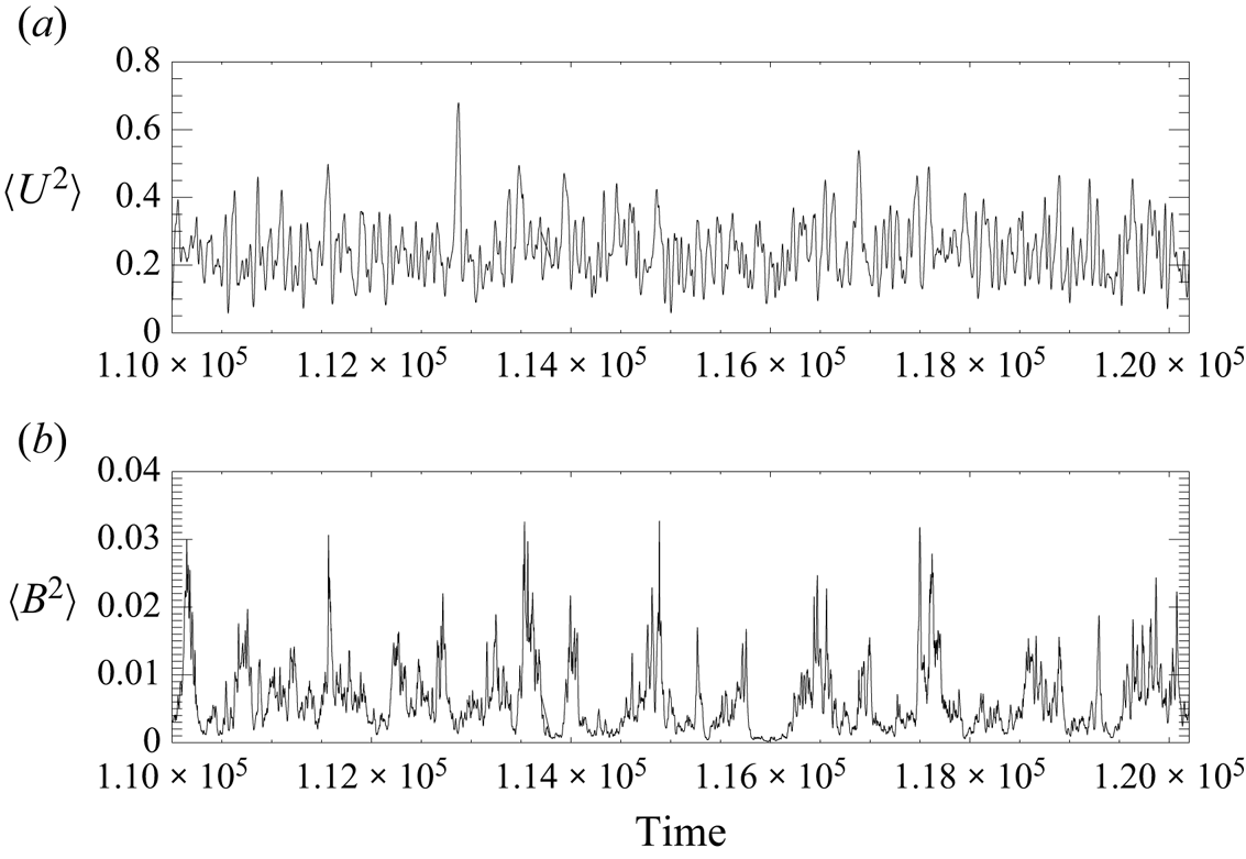
On imposing uniform fields and flows, and in stark contrast to the flows of § 3.1, we find that the solutions to the linear equations (2.7) and (2.8) increase without bound. This is demonstrated by figure 6, which shows the exponential growth, on average, of the e.m.f.s and combined Reynolds and Maxwell stresses calculated from expressions (2.21) and (2.22). As such, the linear theory can give no guide to the mean field coefficients. We thus have to consider the full nonlinear MHD equations (2.23) and (2.24) – for which perturbations are guaranteed to be bounded – and to see whether the average response depends linearly on the imposed mean fields and flows when these are sufficiently small. To provide some insight into the nature of the response of a complicated system to an applied perturbation, we delay to § 5 the discussion of fully nonlinear perturbations in mean field MHD, in order to consider an ostensibly much simpler problem, namely the nature of the response to small symmetry-breaking perturbations of one-dimensional maps.
Components of the mean e.m.f. (a–c) and mean total stress (d–i), calculated from the linear theory, with forcing  $\boldsymbol {F}_1$ and $Re=Rm=100$, after the imposition of a magnetic field of unit magnitude in the $y$-direction.
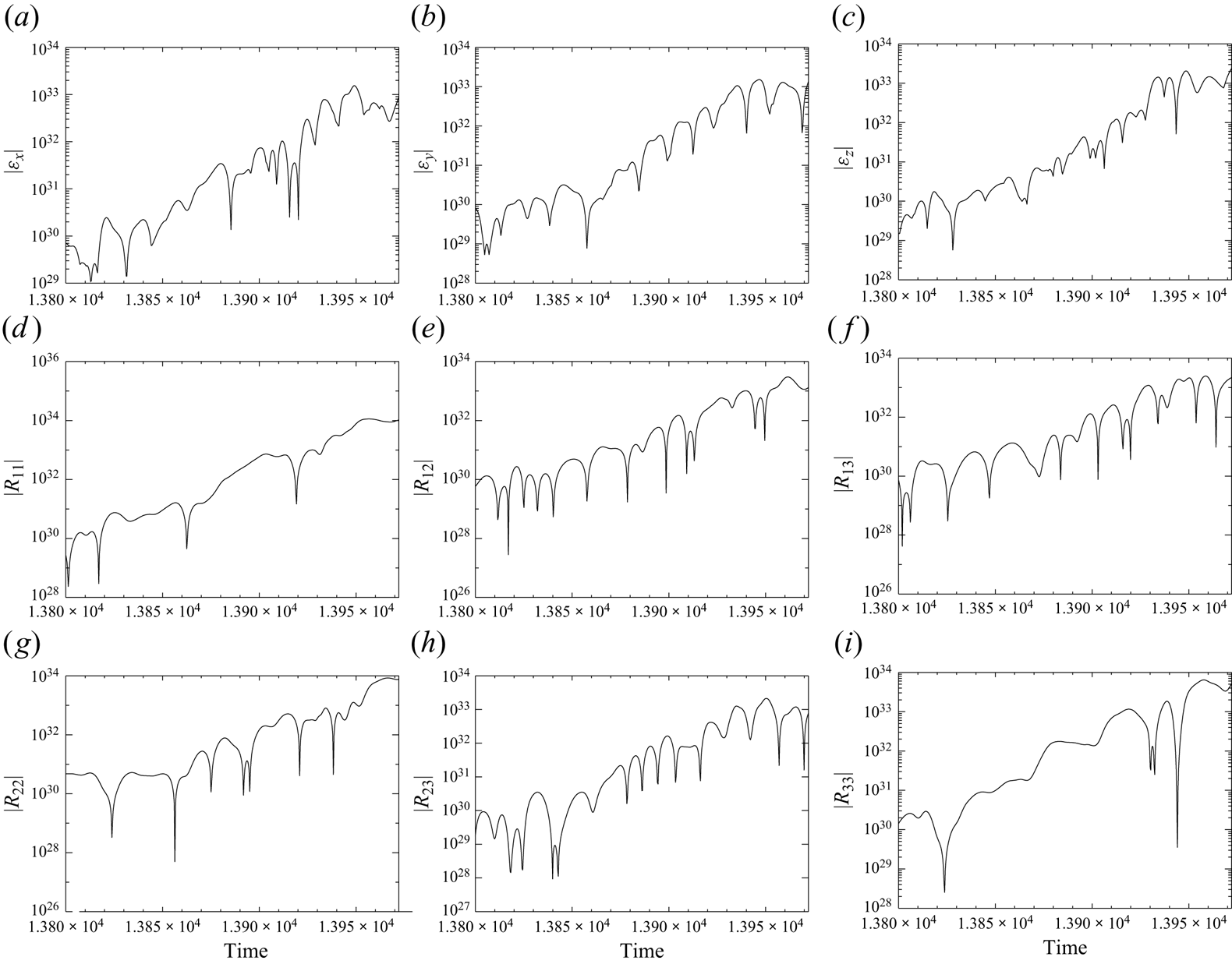
4. Symmetry breaking in one-dimensional maps
In this section, we consider the nature of the response to small symmetry-breaking perturbations of one-dimensional maps. In systems without sensitive dependence on initial conditions, the trajectories of the perturbed system will be close to those of the unperturbed system, and it may therefore be expected that calculations of mean quantities can be accomplished using the linear equations describing the effects of the perturbation. In a chaotic system, on the other hand, excursions of the perturbed trajectories will become large, and so the perturbations can no longer be described by linear equations. However, when averages of quantities are taken over many iterations or large times, the relevant property of the map is the invariant measure (described in detail below), which describes the probability of finding the solution in a given region of phase space. We might hope that this quantity will change only slightly for small perturbations, and so changes to average quantities will scale linearly with the size of the perturbation. There are indeed some systems with special properties for which this hope is realised, but for general systems the required conditions do not hold and the response is not linear. We first give examples of three maps giving both linear and nonlinear responses. Following this, we refer to earlier work to explain how the different behaviours depend on the forms of the maps.
4.1. The invariant measure
The invariant measure (or probability density)  $\mu(x)$ of a map $f(x)$ is specified in the following way. First, we need to know the effect of the map on intervals in the domain. For every point $x$ there is at least one pre-image $\tilde {x}$ such that ${f(\tilde {x})=x}$. The number of pre-images depends on the map, but for a chaotic map there are at least two. An interval $\mathrm {d}\kern0.7pt\tilde {x}$ at $\tilde {x}$ is mapped into an interval ${{\rm d}\kern0.7pt x}=|\,f'(\tilde {x})| \,\mathrm {d}\kern0.7pt\tilde {x}$ at $x$. Thinking of $\mu (x)$ as a (relative) ‘density’ of points in the domain, we can see that the points in the interval ${{\rm d}\kern0.7pt x}$ at $x$ derive from the sum of the quantities $(\mu (\tilde {x}_i)/|\,f'(\tilde {x}_i)|) \,\mathrm {d}\kern0.7pt\tilde {x}$ over the pre-images $\tilde {x}_i$. Since the measure or density is invariant under the map, we have the following functional equation (the Frobenius–Perron equation) determining $\mu (x)$, where the map is defined on the range $-1\leqslant x\leqslant 1$:
 \begin{equation} \mu(x)=\mathop{\sum}\limits_i \frac{\mu(\tilde{x}_i)}{|\,f(\tilde{x}_i)|}\quad{\rm and}\quad\int_{{-}1}^1 \mu(x)\, {{\rm d}\kern0.7pt x}=1. \end{equation}
4.2. Maps with linear response (i): the ‘cubic tent map’
In general,  $\mu (x)$ is very complicated and non-differentiable in nature; see, for example, the plots of $\mu (x)$ for the logistic map in Gottwald, Wormell & Wouters (Reference Gottwald, Wormell and Wouters2016). However, there are some special problems for which both $\mu$ and its dependence on the parameters of the map can be calculated explicitly. As such an example, here we consider the one-parameter family $f(x,a)$ defined on $-1\leqslant x\leqslant 1$ (see figure 7):
 \begin{align}
\left.\begin{array}{@{}l@{\quad}c@{}}
f(x,a) ={-}2-3x & -1 \leqslant x \leqslant -1/3, \\
\phantom{f(x,a)}= 3x & -1/3 \leqslant x \leqslant 0, \\
\phantom{f(x,a)}= ax & 0 \leqslant x \leqslant 1/a, \\
\phantom{f(x,a)}=\dfrac{1+a-2ax}{a-1} & 1/a \leqslant x \leqslant 1.
\end{array}\right\}
\end{align}
\begin{align}
\left.\begin{array}{@{}l@{\quad}c@{}}
f(x,a) ={-}2-3x & -1 \leqslant x \leqslant -1/3, \\
\phantom{f(x,a)}= 3x & -1/3 \leqslant x \leqslant 0, \\
\phantom{f(x,a)}= ax & 0 \leqslant x \leqslant 1/a, \\
\phantom{f(x,a)}=\dfrac{1+a-2ax}{a-1} & 1/a \leqslant x \leqslant 1.
\end{array}\right\}
\end{align}
When  $a=3$ the map is antisymmetric, with the pre-images of $x$ being $x/3$, $(2-x)/3$ and $- (2+x)/3$. Since the gradients of $f(x,a=3)$ at each pre-image have modulus $3$, (4.1a,b) is solved by the constant value $\mu (x)=1/2$. Thus $\langle x\rangle \equiv \int _{-1}^1 x\mu (x)\, {{\rm d} \kern0.7pt x}=0$.
The map  $f(x,a)$ (the cubic tent map, defined by (4.2)), for $a=3$ (red) and $a=5$ (green); the blue line denotes the invariant measure $\mu (x)$ for $a=5$.

For  $a \ne 3$, the (anti-)symmetry of the map is broken, as shown in figure 7. There are now two different (absolute) gradients of the map for positive $x$, and yet a third for $x<0$, and so $\mu$ is no longer constant. However, it turns out that $\mu$ is still piecewise constant, with $\mu =\mu _+$, $x> 0$; $\mu =\mu _-$, $x<0$. For each $x$, there are three pre-images $\tilde {x}_{i}$: for $x>0$, $\tilde {x}_{1}<0$ and $0<\tilde {x}_{2}< a^{-1}<\tilde {x}_{3}<1$, whereas for $x<0$, $\tilde {x}_{1,2}<0$ and $\tilde {x}_{3}>a^{-1}$. The (moduli of the) gradients in $x<0$, $0< x< a_{-1}$, $a_{-1}< x<1$ are $3$,
$3$,  $a$,
$a$,  $2a/(a-1)$, respectively. The assumption of piecewise constancy then leads to the two equations
 \begin{equation} \mu_+=\frac{\mu_-}{3}+\left(\frac{a+1}{2a}\right)\mu_+, \quad \mu_-=\frac{2\mu_-}{3}+\frac{a-1}{2a}\mu_+, \end{equation}
and hence
 \begin{equation} \mu_+=\frac{2a}{5a-3}, \quad \mu_-=\frac{3(a-1)}{5a-3}. \end{equation}
Therefore,
 \begin{equation} \langle x\rangle=\mu_-\int_{{-}1}^{0} x\,{{\rm d}\kern0.7pt x}+\mu_+\int_{0}^{1}x\, {{\rm d}\kern0.7pt x}=\frac{1}{2}(\mu_+-\mu_-)=\frac{3-a}{2(5a-3)}. \end{equation}
Now suppose that  $a=3+\delta$, where $\delta \ll 1$; then, to leading order, $\mu _+\approx (1-\delta /12)/2$, $\mu _-\approx (1+\delta /12)/2$ and $\langle x\rangle \approx -\delta /24$, confirming the linear response. This result can be reproduced by means of a direct perturbation theory.
It should be noted that the perturbation investigated is not the most general. Were we to change the map so that the two peaks were at different heights, then the invariant measure would become non-differentiable, and the situation would be much like that for the cubic logistic map discussed in § 4.4.
4.3. Maps with linear response (ii): the Lorenz map
In the example above, it was possible to compute the invariant measure  $\mu$ explicitly; in general, however, $\mu$ can only be estimated numerically. Here we give an example of a chaotic map, where $\mu$ has to be calculated numerically, and for which the response to small perturbations is indeed linear. The ultra-high resolution computations leading to the results for this map and the following logistic map have been kindly provided by A.M. Rucklidge, and are described in the Appendix.
The Lorenz map, defined by
 \begin{equation} g(x,\mu_0) = \mu_0 + \mathrm{sgn}(x)\left({-}1 + 1.5 \sqrt{|x|} \right), \end{equation}
is chaotic and depends on the parameter  $\mu _0$ in such a way that when $\mu _0=0$, the map is odd and the symmetric chaotic attractor has zero mean. The map, which is shown in figure 8(a), maps the interval $[-1.9,1.9]$ to itself. Having computed the average $\langle {x}\rangle$ for varying $\mu _0$ according to the methods in the Appendix, we can see from figure 9(a) that $\langle {x}\rangle$ is proportional to $\mu _0$ down to $\mu _0=10^{-6}$, below which $\langle {x}\rangle$ is indistinguishable from zero. This linear dependence is in conformity with the results of Bahsoun & Galatolo (Reference Bahsoun and Galatolo2024), who showed that there is a linear response in a tent-like family of maps with a cusp at the turning point.


Average  $\langle {x}\rangle$ as a function of $\mu _0$, averaged over 2000 initial conditions and $10^9$ iterates: (a) Lorenz map; (b,c) cubic logistic map for different ranges of $\mu _0$.

4.4. A map with no linear response: the cubic logistic map
The cubic logistic map, which is shown in figure 8(b), is given by
 \begin{equation} h(x,\mu_0) = \mu_0 + 2.8x - x^3. \end{equation}
Once more, the term in  $\mu _0$ breaks the anti-symmetry.
By comparison with the Lorenz map, the cubic logistic map has an entirely different behaviour as  $\mu _0$ is varied. For larger values of $\mu _0$, above about $2\times 10^{-6}$, $\langle {x}\rangle$ increases with $\mu _0$ (figure 9b). However, for smaller values of $\mu _0$, as shown in figure 9(c), $\langle {x}\rangle$ does not even depend monotonically on $\mu _0$; it changes sign, and is significantly different from zero for all $\mu _0$ down to $10^{-11}$. Certainly, there is no obvious linear dependence.
What are the properties of these maps that give rise to the different behaviours? Baladi (Reference Baladi2014) has given a general treatment of this question, building on earlier work of Ershov (Reference Ershov1993), who considered the invariant measure on tent maps not of ‘full height’. The difference between the behaviours of the logistic and Lorenz maps can be principally ascribed to the form of the invariant measure  $\mu$. For a linear response, $\mu$ has to be sufficiently smooth (e.g. piecewise constant); this can occur when the map is sufficiently mixing. If there are accumulations of discontinuities, for example due to the existence of arbitrarily long-period stable periodic orbits, then there is no smooth response to a small parameter perturbation. The tent map shown is stretching everywhere and has no stable periodic orbits, and $\mu$ is piecewise constant. The Lorenz map is also stretching everywhere, whereas the cubic logistic map, for which the gradient of the map is bounded, has properties similar to the regular logistic map studied by Gottwald et al. (Reference Gottwald, Wormell and Wouters2016), for which there is no linear response.
5. Symmetry breaking in nonlinear MHD (ii): finite-amplitude perturbations
In this section, we return to the MHD problem, and in particular to the case discussed in § 3.2 for which the linear theory fails. We thus consider the response of the MHD system after the imposition of a dynamical magnetic field, and to see whether this response is linear when the field is sufficiently weak. Specifically, we solve (2.23) and (2.24), in concert with (2.1) and (2.2), after the imposition of uniform fields and flows. As an example, figure 10 shows the cumulative averages of the components of the mean e.m.f. and mean total stress calculated from expressions (2.25) and (2.26), after the imposition of a mean magnetic field  $\bar {\boldsymbol {b}} = 10^{-3} \hat {\boldsymbol {y}}$ with no imposed mean flow. It should be noted that the mean e.m.f. and mean stress fluctuate rapidly in time, with root-mean-squared values determined by fast (turbulent) processes. However, as can be seen from the figure, determining a meaningful temporal average requires integration over many thousands of Ohmic (or viscous) diffusion times. Indeed, for quantities such as ${\mathcal {E}}_z$, for which the cumulative average is clearly small, convergence is still elusive. It is clearly necessary to outline a procedure that enables us to extract the mean values from data such as exhibited in figure 10. We first identify a time at which the most exuberant transients have decayed, $t^*$, say, and then average over many Ohmic decay times; over this time interval, denoted by $\mathcal {T}$, say, we calculate the mean and standard deviation. It should though be noted that an unambiguous identification of $t^*$ is not straightforward, since, as can be seen from figure 10, the different components of the mean field tensors converge at different rates. It can be seen that for the particular case of an imposed mean field $\bar {\boldsymbol {b}} = 10^{-3} \hat {\boldsymbol {y}}$, the cumulative average for ${\mathcal {E}}_y$ has settled down by $t=1.5 \times 10^5$, and so we may adopt this time as a not unreasonable choice for $t^*$; with this choice, we then average from $t=t^*=1.5 \times 10^5$ to $t=t^*+ {\mathcal {T}} = 2.2 \times 10^5$, corresponding to $O(700)$ Ohmic decay times.
Cumulative averages of the components of the mean e.m.f. (a–c) and mean total stress (d–i), normalised by the mean field strength  $b = |\bar{\boldsymbol {b}}|$, calculated from the nonlinear MHD equations, with forcing $\boldsymbol {F}_1$ and $Re=Rm=100$, after the imposition of a mean magnetic field $\bar {\boldsymbol {b}} = 10^{-3} \hat {\boldsymbol {y}}$.

In order to detect whether the response is linear in the imposed field, it is necessary to conduct numerical simulations for a range of imposed field strengths  $|\bar {\boldsymbol {b}}|$. Figure 11 shows the mean and standard deviation for all components of the e.m.f. and stress (normalised by $|\bar {\boldsymbol {b}}|$) as functions of $|\bar {\boldsymbol {b}}|$ (as in figure 10, the imposed field is in the $y$-direction, with no imposed flow; $t^*$ and $\mathcal {T}$ are identified individually for each value of $|\bar {\boldsymbol {b}}|$). We note that the dominant component of the e.m.f. is ${\mathcal {E}}_y$ (i.e. the component of ${\boldsymbol{\mathcal{E}}}$ in the direction of $\bar {\boldsymbol {b}}$), with ${\mathcal {E}}_y/|\bar {\boldsymbol {b}}|$ tending to a (non-zero) constant as $|\bar {\boldsymbol {b}}| \to 0$ (i.e. a linear response). Although there is some scatter in the values of ${\mathcal {E}}_x$ and ${\mathcal {E}}_z$, their values are small, and not inconsistent with being zero. Similar behaviour for imposed fields in the $x$- and $z$-directions (i.e. the dominant component of the e.m.f. in the direction of the imposed field) would imply that $\boldsymbol {\alpha }^{(1)}$ is diagonal. The picture for the components of the total stress is, unfortunately, less clear. The three diagonal entries of $R_{ij}$ have relatively small error bars; $R_{11}$ is consistent with a linear response, whereas $R_{22}$ and $R_{33}$ are not. The values of the off-diagonal components are small, with larger error bars, and are not inconsistent with being zero. It is by no means obvious why the components of the stress are less well-behaved than those of the e.m.f. However, calculation of the stress $R_{ij}$, given by (2.25), reveals that the linear and nonlinear terms are almost offsetting, with the residual stress being much smaller than its constituent parts; therefore, the less robust behaviour of the stress is not altogether unsurprising.
Components of the mean e.m.f. (a–c) and mean total stress (d–i), normalised by the mean field strength  $b=|\bar{\boldsymbol {b}}|$, vs b; the imposed field is in the $y$-direction. The circles denote the mean values, obtained by averaging over the interval $\mathcal {T}$; the error bars are $\pm 1$ standard deviation.

Since the clearest linear response is in the e.m.f., it is of interest, as noted above, to vary the direction of the imposed magnetic field. Figure 12 shows the components of the e.m.f. in the direction of the imposed field for a range of field strengths  $|\bar {\boldsymbol {b}}|$ and for imposed fields in the $x$-,
$x$-,  $y$- and $z$-directions. For a range of sufficiently small $|\bar {\boldsymbol {b}}|$, there is indeed a linear response in all cases. This allows us to calculate the diagonal elements of $\boldsymbol {\alpha }^{(1)}$; these can be read off from the right-hand column in figure 12, which shows the values of the e.m.f.s normalised by $|\bar {\boldsymbol {b}}|$, as $\alpha ^{(1)}_{11} \approx -0.14$ and $\alpha ^{(1)}_{22} \approx \alpha ^{(1)}_{33} \approx -0.1$. The fact that the diagonal elements of $\boldsymbol {\alpha }^{(1)}$ are not all equal reflects a slight lack of isotropy in the basic state.
(a,c,e) Component of the e.m.f. in the direction of the imposed field vs the strength of the field  $b= |\bar {\boldsymbol {b}}|$. (b,d,f) Same quantity divided by b. In (a,b), the imposed field is in the $x$-direction, in (c,d) the $y$-direction and in (e,f) the $z$-direction; there is no imposed mean flow. The dotted line has unit slope, corresponding to a linear response.

The discussion above has considered the mean field response following imposition of a uniform magnetic field. In theory, assuming a linear response, this would allow us to determine  $\boldsymbol {\alpha }^{(1)}$ and $\boldsymbol {\varGamma }^{(2)}$; in practise, the lack of a clear linear response in the stress makes the determination of $\boldsymbol {\varGamma }^{(2)}$ problematic. Similarly, imposition of a uniform flow in theory allows the determination of $\boldsymbol {\alpha }^{(2)}$ and $\boldsymbol {\varGamma }^{(1)}$. The values of the e.m.f.s are found to be small, suggesting that, as in the case with lower Reynolds numbers (see § 3.1), $\boldsymbol {\alpha }^{(2)}$ is not a significant player. Again, as for imposed fields, it is difficult to establish a linear response of the stress to imposed flows; thus, the determination of $\boldsymbol {\varGamma }^{(1)}$ is similarly problematic.
6. Conclusions and discussion
Our chief goal in this paper has been to explore the concrete consequences of the formalism introduced by Courvoisier et al. (Reference Courvoisier, Hughes and Proctor2010a) to describe long-wavelength instabilities of self-consistent three-dimensional MHD states. In § 2.1, we recapitulate the formal development of the mean field equations. Only in special cases is it possible to obtain explicit expressions for the mean field tensors  $\boldsymbol {\alpha }^{(1)}$, $\boldsymbol {\alpha }^{(2)}$, $\boldsymbol {\varGamma }^{(1)}$ and $\boldsymbol {\varGamma }^{(2)}$. One such example, the case of short-sudden turbulence, is described in § 2.2. The formalism of § 2.1 is designed to capture the mean field tensors on the basis of linearised equations for the fluctuating fields and flows, following the classical approach of mean field MHD. This works well for sufficiently smooth basic states. In § 3.1 we demonstrate the linear response for two such cases, and show how the results can be used to predict long-wavelength instability. However, the approach can fail for more disordered flows and fields, for which the linearised perturbations can grow exponentially. In this case, to ensure that the fluctuations are bounded, we restore the nonlinear terms in the perturbation equations. It is then of interest to discover the nature of the mean response to small imposed mean fields and flows and to ascertain whether this is indeed linear. The question of a possible linear mean response to perturbations of a nonlinear system has been widely studied in a number of contexts. To illustrate these ideas in a relatively simple system, we consider in § 4 several one-dimensional maps, of varying character, and show that in some cases there is a well-defined mean linear response, whereas in others there is not. In § 5, we return to the MHD problem and consider a more complicated basic state, in which nonlinear perturbations have to be included to ensure a bounded response.
It is of interest to note that the simple maps for which the response of averages is a linear function of small perturbations have the property that they are stretching everywhere. On the other hand, for the MHD problem, it is the fields and flows considered here with minimal or no chaos, for which linear theory works well. In this case, we may readily extract the mean field tensors and, consequently, determine the stability of the basic state to long-wavelength perturbations. It may be verified from the full equations that for small imposed fields and flows the mean response in this case is linear, as might be expected. For the models with disordered fields and flows, on the other hand, the linearised perturbation theory fails and the averages grow without limit. Restoration of the nonlinearities guarantees that the perturbations remain bounded and so averages can, in principle, be determined. The difficulty here lies in extracting the small signal (the mean) from the large fluctuations, as previously discussed by Cattaneo & Hughes (Reference Cattaneo and Hughes2006) and Hughes & Cattaneo (Reference Hughes and Cattaneo2008). All this makes it difficult to determine unambiguously the precise nature of the response.
Acknowledgements
We are grateful to A. Courvoisier for helpful discussions at the onset of this research, and to A.M. Rucklidge, who carried out the computations for the maps depicted in figure 9, and provided the commentary on the numerical methods in the Appendix. We thank the referees for their insightful reports, which helped to improve the paper. The authors would like to thank the Isaac Newton Institute for Mathematical Sciences, Cambridge, for support and hospitality during the programme Anti-diffusive dynamics: from sub-cellular to astrophysical scales, where work on this paper was undertaken.
Funding
This work was supported by EPSRC grant EP/R014604/1. This work used the DiRAC Complexity system, operated by the University of Leicester IT Services, which forms part of the STFC DiRAC HPC Facility. This equipment is funded by BIS National E-Infrastructure capital grant ST/K000373/1 and STFC DiRAC Operations grant ST/K0003259/1; DiRAC is part of the National E-Infrastructure.
Declaration of interests
The authors report no conflict of interest.
Appendix
Here we describe the nature of the computations needed for an accurate determination of averages for the one-dimensional maps discussed in § 4.
For the Lorenz map, we took 2000 initial conditions for  $x$, spread across the interval $[0.01,0.99]$, with values of $\mu _0$ in the range $10^{-12}$ to $10^{-2}$, and computed $10^9$ iterates of each map, for each initial condition and for each choice of $\mu _0$. For a given value of $\mu _0$ and each initial condition, averages were taken over the entire run. The resulting distribution of 2000 values is well represented by a Gaussian, so we used the mean and standard deviation of the distribution to estimate $\langle {x}\rangle$ and its error. In this case, the error is typically $4\times 10^{-7}$. The cubic logistic map was treated in the same way; in that case the error is $10^{-6}$.
These calculations are delicate, and require the use of high-precision arithmetic in order to compute the map reliably, particularly in the case of the cubic logistic map. In any finite-precision numerical computation of this type, maps are not strictly chaotic but rather have long-period periodic orbits, owing to the limited number of binary digits in the representation of real numbers. A 52-bit mantissa in double precision should mean of the order of  $10^{15}$ different numbers being available. However, in the case of maps with quadratic maxima, for example the cubic logistic map, the number of different trajectories is significantly reduced because near the maximum, the function (in double precision) looks like a series of broad steps up and down, and so the range of possible outcomes for trajectories that approach the maximum is also much reduced. For example, in double precision arithmetic, the behaviour of the cubic logistic map with $\mu _0=0$ is dominated by a periodic orbit with period on the order of $3\times 10^7$. This orbit is symmetric and has $\langle {x}\rangle =0$. The majority of initial conditions converge to this orbit after a transient of up to $10^8$ iterates. However, a small fraction of initial conditions (about 0.4 %) converge to other periodic orbits, some of which have non-zero mean. This clearly means that an average of $10^9$ iterates of the map, computed in double precision, is not sampling the chaotic attractor. There are similar issues with non-zero $\mu _0$. As a result, double precision calculations cannot be relied on here, and we carried out our computations in extended precision arithmetic (using the GNU Multiple Precision Arithmetic Library gmp), specifying a 256-bit mantissa. The results we present in figure 9 are not sensitive to the choice of mantissa length, provided that it is sufficiently large.


 Open access