


1. Introduction
Thermal convection is ubiquitous in various natural and engineering applications, such as thermal management in batteries and aerospace (Wu et al. Reference Wu, Wang, Wu, Chen, Hong and Lai2019; Xue et al. Reference Xue, Wang, Yue, Lian, Zhang and Gao2024), heat exchangers (Garoosi, Hoseininejad & Rashidi Reference Garoosi, Hoseininejad and Rashidi2016) and food processing (Ghani et al. Reference Abdul Ghani, Farid, Chen and Richards1999). Rayleigh–Bénard convection (RBC) is one of the canonical models that has been used extensively to investigate important issues related to heat transport and flow dynamics due to its generality and simple configuration, where a closed domain of fluid is subject to heating from the bottom and cooling from the top, while the sidewalls remain adiabatic (Bodenschatz, Pesch & Ahlers Reference Bodenschatz, Pesch and Ahlers2000; Ahlers, Grossmann & Lohse Reference Ahlers, Grossmann and Lohse2009). The cooled fluid near the top plate is denser than the heated fluid near the bottom, generating a gravitational instability. For a given geometry, the RBC is governed by two dimensionless parameters: the Rayleigh number $Ra$
, which quantifies the strength of the thermal driving force compared with the viscous dissipative force, and the Prandtl number
$Ra$
, which quantifies the strength of the thermal driving force compared with the viscous dissipative force, and the Prandtl number $\textit{Pr}$
, which characterises the relative diffusivities of momentum and heat. It has been reported in previous studies that when
$\textit{Pr}$
, which characterises the relative diffusivities of momentum and heat. It has been reported in previous studies that when $Ra$
is below the critical threshold
$Ra$
is below the critical threshold $Ra_T$
– approximately 1708 for classical RBC in an infinitely wide cavity (Koschmieder Reference Koschmieder1993) and approximately 2415 for RBC in an enclosed cavity (Huang & Zhang Reference Huang and Zhang2023) – the fluid is static, and heat is transferred through conduction only. When
$Ra_T$
– approximately 1708 for classical RBC in an infinitely wide cavity (Koschmieder Reference Koschmieder1993) and approximately 2415 for RBC in an enclosed cavity (Huang & Zhang Reference Huang and Zhang2023) – the fluid is static, and heat is transferred through conduction only. When $Ra$
is increased well beyond the critical value, the well-known scaling law
$Ra$
is increased well beyond the critical value, the well-known scaling law $\textit{Nu} \propto Ra^{\gamma }$
has been proposed to describe the relationship between heat transfer and the imposed buoyancy effects, where
$\textit{Nu} \propto Ra^{\gamma }$
has been proposed to describe the relationship between heat transfer and the imposed buoyancy effects, where $Nu$
is the Nusselt number defined as the ratio between the convective and conductive heat transfer rates (Grossmann & Lohse Reference Grossmann and Lohse2000; Ahlers et al. Reference Ahlers, Grossmann and Lohse2009). A key direction in RBC research is to explore different ways of manipulating the heat transfer and modifying the scaling exponent
$Nu$
is the Nusselt number defined as the ratio between the convective and conductive heat transfer rates (Grossmann & Lohse Reference Grossmann and Lohse2000; Ahlers et al. Reference Ahlers, Grossmann and Lohse2009). A key direction in RBC research is to explore different ways of manipulating the heat transfer and modifying the scaling exponent $\gamma$
at a given
$\gamma$
at a given $Ra$
. This has important practical implications for applications where controlled modulation of heat transfer is essential, including thermal management, energy conservation and ventilation. Numerous approaches have been developed to achieve this objective. For example, previous studies have shown that adding insulating partitions within the domain (Bao et al. Reference Bao, Chen, Liu, She, Zhang and Zhou2015) or tilting the convection cell (Guo et al. Reference Guo, Zhou, Cen, Qu, Lu, Sun and Shang2015) can modify the fluid circulation and increase the heat transfer rate. It is also found that changing the surface roughness of the isothermal plates can lead to higher heat transfer efficiency (Tummers & Steunebrink Reference Tummers and Steunebrink2019). In addition, Chong et al. (Reference Chong, Yang, Huang, Zhong, Stevens, Verzicco, Lohse and Xia2017) realised the enhancement of heat transfer through coherent structure manipulation.
$Ra$
. This has important practical implications for applications where controlled modulation of heat transfer is essential, including thermal management, energy conservation and ventilation. Numerous approaches have been developed to achieve this objective. For example, previous studies have shown that adding insulating partitions within the domain (Bao et al. Reference Bao, Chen, Liu, She, Zhang and Zhou2015) or tilting the convection cell (Guo et al. Reference Guo, Zhou, Cen, Qu, Lu, Sun and Shang2015) can modify the fluid circulation and increase the heat transfer rate. It is also found that changing the surface roughness of the isothermal plates can lead to higher heat transfer efficiency (Tummers & Steunebrink Reference Tummers and Steunebrink2019). In addition, Chong et al. (Reference Chong, Yang, Huang, Zhong, Stevens, Verzicco, Lohse and Xia2017) realised the enhancement of heat transfer through coherent structure manipulation.
Although the above examples show the potential of controlling the heat transfer, most of them involve changing the geometry or adding mechanical parts. In certain applications, an active control of heat transfer without introducing moving parts is more desirable. Recently, Huang & Zhang (Reference Huang and Zhang2023) numerically investigated the influence of adding a horizontal heat flux through a pair of heating–cooling vertical walls on heat transfer, which demonstrated a significant enhancement of large-scale circulation and heat transfer in RBC. However, the authors subsequently noted that this approach requires the simultaneous addition and removal of equal amounts of heat, a condition that is practically unattainable in experiments (Huang & Zhang Reference Huang and Zhang2024). Consequently, in a later study, they experimentally investigated the influence of side heating on the flow dynamics and thermal convection, and reported a monotonic increase in the heat transfer with the applied side-heating power (Huang & Zhang Reference Huang and Zhang2024). Both the numerical and experimental work provide a simple way of controlling heat transfer in RBC without changing the geometry.
Another common strategy for actively manipulating heat transfer is the injection of unipolar electric charges, a process generally referred to as electro-thermo-convection. When a dielectric fluid is confined between two electrodes and subjected to an applied voltage, space charges are injected into the fluid via electrochemical reactions at the metal–fluid interface. The resulting interaction between the electric field and these charges produces a Coulomb force, which modifies the flow behaviour and consequently the heat transfer (Denat, Gosse & Gosse Reference Denat, Gosse and Gosse1979). Previous studies have demonstrated that charge injection can effectively enhance heat transfer in classical RBC (Traore et al. Reference Traore, Pérez, Koulova and Romat2010; Luo et al. Reference Luo, Wu, Yi and Tan2016; Gao et al. Reference Gao, Zhang, Zhang and Zhang2019; Lu, Liu & Wang Reference Lu, Liu and Wang2019; Jiang et al. Reference Jiang, Zhang, Zhang, Luo and Yi2022; Wu et al. Reference Wu, Wang, Lu and Zhou2022). In addition, numerical studies have further shown that alternately arranged electrodes yield greater heat transfer enhancement than configurations in which a wall is fully covered with identical electrodes (either all positive or all grounded) (Son & Park Reference Son and Park2021). However, most existing studies remain largely parametric and provide limited physical insight into the underlying mechanisms.
Although the individual effects of sidewall heating and charge injection have been extensively studied, their combined influence on heat transfer, flow organisation and the underlying physical mechanisms remains largely unexplored. Furthermore, the complex interplay between the buoyancy and Coulomb forces gives rise to intricate flow structures and dynamics, leading to highly nonlinear and unpredictable flow behaviours. Elucidating these mechanisms is therefore crucial for achieving effective control of the system. In this work, we investigate heat transfer and flow structures under the coupled effects of sidewall heating and unipolar charge injection from the bottom wall. Applying these two effects at different boundaries allows the interaction between buoyancy-driven circulation and Coulomb-driven forcing to be diagnosed cleanly to clarify how two spatially distinct driving mechanisms interact with each other. Through extensive simulations, the current work aims to enhance our understanding of the fundamental aspects of nonlinear interaction between the additional buoyancy force from the sidewall and Coulomb force with emphasis on the heat transfer regime and flow structure transition.
2. Problem description
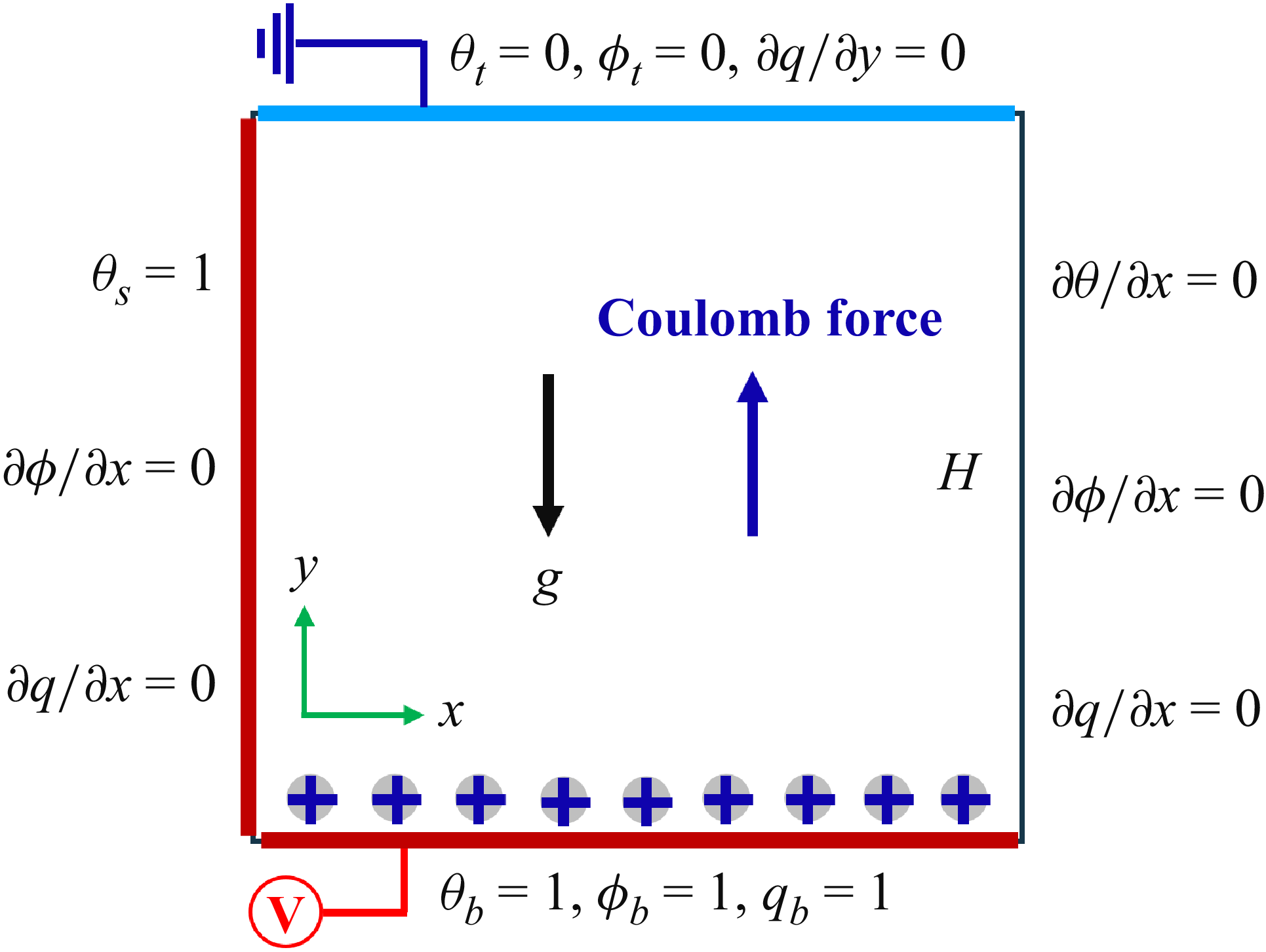
The problem configuration is shown in figure 1. An incompressible, Newtonian, perfectly dielectric fluid is considered within a square cavity of height $H$
, bounded by two parallel, horizontally aligned electrodes. The top and bottom walls are maintained at constant but distinct electric potentials and temperatures, with the bottom wall set to a higher potential and temperature (
$H$
, bounded by two parallel, horizontally aligned electrodes. The top and bottom walls are maintained at constant but distinct electric potentials and temperatures, with the bottom wall set to a higher potential and temperature ( $\phi _b=1$
and
$\phi _b=1$
and $\theta _b=1$
), while the top is kept at a lower potential and temperature (
$\theta _b=1$
), while the top is kept at a lower potential and temperature ( $\phi _t=0$
and
$\phi _t=0$
and $\theta _t=0$
). Furthermore, the left wall is maintained at the same temperature as the bottom wall (
$\theta _t=0$
). Furthermore, the left wall is maintained at the same temperature as the bottom wall ( $\theta _s=\theta _b=1$
). The charge injection is considered to occur exclusively at the bottom electrode (i.e. unipolar injection) due to the electrochemical reaction at the liquid–electrode interface, with a constant injected charge density (
$\theta _s=\theta _b=1$
). The charge injection is considered to occur exclusively at the bottom electrode (i.e. unipolar injection) due to the electrochemical reaction at the liquid–electrode interface, with a constant injected charge density ( $q_b=1$
). The no-slip boundary conditions, namely
$q_b=1$
). The no-slip boundary conditions, namely $\boldsymbol{u}=0$
, are applied to all walls. Under the Boussinesq approximation (Rayleigh Reference Rayleigh1916), the dimensionless equations governing the system described above include the incompressible Navier–Stokes equations for Newtonian fluid, the energy equation for temperature, the Poisson equation for electric potential and the Nernst–Planck equation for the charge transport, which can be written as
$\boldsymbol{u}=0$
, are applied to all walls. Under the Boussinesq approximation (Rayleigh Reference Rayleigh1916), the dimensionless equations governing the system described above include the incompressible Navier–Stokes equations for Newtonian fluid, the energy equation for temperature, the Poisson equation for electric potential and the Nernst–Planck equation for the charge transport, which can be written as
 \begin{equation} \boldsymbol{\nabla }\boldsymbol{\cdot }\boldsymbol{u}=0, \end{equation}
 \begin{equation} \frac {\partial (\boldsymbol{u})}{\partial t} + \boldsymbol{\nabla }\boldsymbol{\cdot }(\boldsymbol{u u}) = -\boldsymbol{\nabla }\! p + {\nabla} ^2 \boldsymbol{u} + \frac {T^2}{M^2} q C \boldsymbol{\cdot }\boldsymbol{E} + \frac {Ra}{\textit{Pr}} \theta \boldsymbol{\cdot }\boldsymbol{e_y}, \end{equation}
 \begin{equation} \frac {\partial \theta }{\partial t} + \boldsymbol{u} \boldsymbol{\cdot }\boldsymbol{\nabla }\theta = \frac {1}{\textit{Pr}} {\nabla} ^2 \theta , \end{equation}
 \begin{equation} {\nabla} ^2 \phi = -q C, \end{equation}
 \begin{equation} \boldsymbol{E} = -\boldsymbol{\nabla }(\phi ), \end{equation}
 \begin{equation} \frac {\partial q}{\partial t} + \boldsymbol{\nabla }\boldsymbol{\cdot }\left[\left(\frac {T}{M^2} \boldsymbol{E} + \boldsymbol{u}\right) q\right] = \alpha {\nabla} ^2 q, \end{equation}
where vectors $\boldsymbol{u}=(u_x, \; u_y)$
and
$\boldsymbol{u}=(u_x, \; u_y)$
and $\boldsymbol{E}=(E_x,\;E_y)$
represent the velocity field and electric field, respectively,
$\boldsymbol{E}=(E_x,\;E_y)$
represent the velocity field and electric field, respectively, $\boldsymbol{e_y}=[0,\;1]$
is a unit vector in the
$\boldsymbol{e_y}=[0,\;1]$
is a unit vector in the $y$
direction and
$y$
direction and $\rho$
,
$\rho$
, $p$
,
$p$
, $\phi$
,
$\phi$
, $q$
and
$q$
and $\theta$
denote the fluid density, pressure, electric potential, charge density and temperature, respectively.
$\theta$
denote the fluid density, pressure, electric potential, charge density and temperature, respectively.
Simulation set-up. The temperatures at the bottom $\theta _b$
and left side boundaries
$\theta _b$
and left side boundaries $\theta _s$
are maintained at the same value, namely
$\theta _s$
are maintained at the same value, namely $\theta _b = \theta _s = 1$
. The top boundary is cold
$\theta _b = \theta _s = 1$
. The top boundary is cold $\theta _t=0$
, and the right boundary is adiabatic. The positive unipolar electric charge is injected from the bottom (
$\theta _t=0$
, and the right boundary is adiabatic. The positive unipolar electric charge is injected from the bottom ( $\phi _b=1, q_b=1$
) with the top wall grounded (
$\phi _b=1, q_b=1$
) with the top wall grounded ( $\phi _t=0$
).
$\phi _t=0$
).

Based on the above formulas, the dimensionless parameters controlling the system are shown as follows:
 \begin{align} Ra = \frac {g \beta \Delta \theta H^3}{\nu \chi }, \; \; \textit{Pr} = \frac {\nu }{\chi }, \; \; \varGamma = \frac {L}{H}, \; \; T =\frac {\varepsilon \Delta \phi }{\mu K}, \; \; C = \frac {q_0 H^2}{\varepsilon \Delta \phi }, \; \; M = \frac {1}{K}\left(\frac {\varepsilon }{\rho }\right)^{\frac {1}{2}}\!, \; \; \alpha = \frac {D}{K\Delta \phi }. \end{align}
In (2.7), the physical properties $g$
,
$g$
, $\mu$
,
$\mu$
, $\beta$
,
$\beta$
, $\chi$
,
$\chi$
, $\varepsilon$
,
$\varepsilon$
, $K$
and
$K$
and $D$
stand for the gravitational acceleration, dynamic viscosity, thermal expansion coefficient, thermal diffusivity, electrical permittivity, ionic mobility and charge-diffusion coefficient. The Rayleigh number
$D$
stand for the gravitational acceleration, dynamic viscosity, thermal expansion coefficient, thermal diffusivity, electrical permittivity, ionic mobility and charge-diffusion coefficient. The Rayleigh number $Ra$
represents the ratio of the buoyancy force to the viscous force. The Prandtl number
$Ra$
represents the ratio of the buoyancy force to the viscous force. The Prandtl number $\textit{Pr}$
, defined as the ratio of momentum to thermal diffusivity, is set to 7 in all simulations. The aspect ratio
$\textit{Pr}$
, defined as the ratio of momentum to thermal diffusivity, is set to 7 in all simulations. The aspect ratio $\varGamma$
is defined as the ratio of the length
$\varGamma$
is defined as the ratio of the length $L$
to the height
$L$
to the height $H$
of the convection cell. In this work, the aspect ratio
$H$
of the convection cell. In this work, the aspect ratio $\varGamma$
is fixed at 1. The electric Rayleigh number
$\varGamma$
is fixed at 1. The electric Rayleigh number $T$
is defined as the ratio of the Coulomb force to the viscous force,
$T$
is defined as the ratio of the Coulomb force to the viscous force, $C$
stands for the charge-injection strength,
$C$
stands for the charge-injection strength, $M$
represents the ratio of the hydrodynamic mobility and the ion mobility and it only depends on the physical properties of the fluid and
$M$
represents the ratio of the hydrodynamic mobility and the ion mobility and it only depends on the physical properties of the fluid and $\alpha$
denotes the dimensionless charge-diffusion number, whose typical value ranges between
$\alpha$
denotes the dimensionless charge-diffusion number, whose typical value ranges between $10^{-4}$
and
$10^{-4}$
and $10^{-3}$
(Pérez & Castellanos 1989). We use
$10^{-3}$
(Pérez & Castellanos 1989). We use $\alpha =10^{-4}$
in our study. The boundary conditions for the hydrodynamic, temperature and electric field are shown in figure 1.
$\alpha =10^{-4}$
in our study. The boundary conditions for the hydrodynamic, temperature and electric field are shown in figure 1.
The unified lattice Boltzmann method (Luo et al. Reference Luo, Wu, Yi and Tan2016) is employed to solve the above equations. Specifically, four consistent lattice Boltzmann equations with two dimensional and nine velocity lattice structures are formulated for solving the flow field, temperature field, electric potential and charge transport, namely, (2.1)–(2.6). A detailed description of the numerical model can be found in Luo et al. (Reference Luo, Wu, Yi and Tan2016) and in our previous studies (Zhao et al. Reference Zhao, Wang, Gu and Sauret2023, Reference Zhao, Wang and Sauret2024; Zhang et al. Reference Zhang, Dzanic, Zhao, Qian, Sun, Zhan, Gu, Sauret and Lü2025), and is therefore omitted here for brevity. The validation of the numerical model is provided in Appendix A.
3. Results and discussion
3.1. Transient and averaged spatial distribution of the temperature and electric charge
Each simulation runs for 8 million time steps, which corresponds to the dimensionless time $t^*=t/(H^2/\nu )=8.4$
, where
$t^*=t/(H^2/\nu )=8.4$
, where $\nu$
is the kinematic viscosity. The time-averaged quantities, such as temperature
$\nu$
is the kinematic viscosity. The time-averaged quantities, such as temperature $\theta$
, electric charge
$\theta$
, electric charge $q$
and
$q$
and $\textit{Nu}$
, are averaged during the latter 4 million time steps, where the system has equilibrated. First, figures 2(a) and 2(b) display the instantaneous temperature, velocity and charge fields at the characteristic time
$\textit{Nu}$
, are averaged during the latter 4 million time steps, where the system has equilibrated. First, figures 2(a) and 2(b) display the instantaneous temperature, velocity and charge fields at the characteristic time $t^* =5$
for a low Rayleigh number
$t^* =5$
for a low Rayleigh number $Ra=100$
and a high electric Rayleigh number
$Ra=100$
and a high electric Rayleigh number $T=1000$
. It is well established that, for pure thermoconvection (
$T=1000$
. It is well established that, for pure thermoconvection ( $T=0$
), a steady state is attained at
$T=0$
), a steady state is attained at $Ra = 100$
. Our results show that a sufficiently strong electric field can induce turbulent flows at low
$Ra = 100$
. Our results show that a sufficiently strong electric field can induce turbulent flows at low $Ra$
. As depicted in figure 2(a), two vortices emerge, and the temperature field exhibits pronounced spatial fluctuations. Correspondingly, similar behaviours can also be observed in the electric charge field. The charge plumes along the sidewalls, originating from the bottom wall, emit downward dissipative structures into the charge void region. This behaviour arises because the impinging plumes generate a corner vortex, as shown in figure 2(a). This vortex deflects the sidewall plumes toward the central region, where they descend and diffuse into the charge void region.
$Ra$
. As depicted in figure 2(a), two vortices emerge, and the temperature field exhibits pronounced spatial fluctuations. Correspondingly, similar behaviours can also be observed in the electric charge field. The charge plumes along the sidewalls, originating from the bottom wall, emit downward dissipative structures into the charge void region. This behaviour arises because the impinging plumes generate a corner vortex, as shown in figure 2(a). This vortex deflects the sidewall plumes toward the central region, where they descend and diffuse into the charge void region.
(a) Representative transient temperature and velocity field, and (b) electric charge field at $t^*=5$
,
$t^*=5$
, $Ra=100$
and
$Ra=100$
and $T=1000$
.
$T=1000$
.

To illustrate the transient and turbulent characteristics of the fluid flow and heat transfer, the temporal evolution of the Reynolds number $Re_A=U_{\mathrm{max}}H/\nu$
, where the maximum velocity
$Re_A=U_{\mathrm{max}}H/\nu$
, where the maximum velocity $U_{\mathrm{max}}=\mathrm{max}|\boldsymbol{u}|$
, is depicted in figure 3(a). It clearly shows that the flow field varies chaotically and exhibits turbulent behaviours at
$U_{\mathrm{max}}=\mathrm{max}|\boldsymbol{u}|$
, is depicted in figure 3(a). It clearly shows that the flow field varies chaotically and exhibits turbulent behaviours at $Ra=100$
and
$Ra=100$
and $T=1000$
. In addition, the black line in figure 3(b) shows the spatially averaged Nusselt number along the top wall, defined as
$T=1000$
. In addition, the black line in figure 3(b) shows the spatially averaged Nusselt number along the top wall, defined as $\textit{Nu}_A = -({1}/{H})\int _0^H \partial _y \theta (x,H)\mathrm{d}x$
, which characterises the total heat transfer rate. This further confirms that, at low buoyancy effect (
$\textit{Nu}_A = -({1}/{H})\int _0^H \partial _y \theta (x,H)\mathrm{d}x$
, which characterises the total heat transfer rate. This further confirms that, at low buoyancy effect ( $Ra = 100$
), the flow can become turbulent and exhibit high-frequency oscillations at high electric Rayleigh number
$Ra = 100$
), the flow can become turbulent and exhibit high-frequency oscillations at high electric Rayleigh number $T = 1000$
. The moving average of
$T = 1000$
. The moving average of $\textit{Nu}_A$
over a window of 1000 data points is shown as the red line in figure 3(b). Its near-constant profile indicates that, despite substantial instantaneous fluctuations, the long-term average
$\textit{Nu}_A$
over a window of 1000 data points is shown as the red line in figure 3(b). Its near-constant profile indicates that, despite substantial instantaneous fluctuations, the long-term average $\textit{Nu}_A$
remains approximately steady.
$\textit{Nu}_A$
remains approximately steady.
(a) Time series of the averaged Reynolds number $Re_A$
. (b) Time series of the averaged Nusselt number
$Re_A$
. (b) Time series of the averaged Nusselt number $\textit{Nu}_A$
. The red line represents the moving average of
$\textit{Nu}_A$
. The red line represents the moving average of $\textit{Nu}_A$
. The values of
$\textit{Nu}_A$
. The values of $Ra$
and
$Ra$
and $T$
are the same as those in figure 2.
$T$
are the same as those in figure 2.

Figures 4(a) and 4(b) show the contours of the averaged dimensionless temperature and electric charge for different $Ra$
and
$Ra$
and $T$
. The case of
$T$
. The case of $T=0$
corresponds to pure thermal convection without charge injection. At low and moderate Rayleigh numbers (
$T=0$
corresponds to pure thermal convection without charge injection. At low and moderate Rayleigh numbers ( $Ra = 10^2$
and
$Ra = 10^2$
and $10^4$
), two thermal plumes begin to emerge near the top-left and bottom-right corners of the cavity as
$10^4$
), two thermal plumes begin to emerge near the top-left and bottom-right corners of the cavity as $T$
increases. The thermal plume originating from the bottom-right corner rises upward as the electric field becomes increasingly dominant. As
$T$
increases. The thermal plume originating from the bottom-right corner rises upward as the electric field becomes increasingly dominant. As $Ra$
increases further, namely
$Ra$
increases further, namely $Ra=10^6$
, the influence of
$Ra=10^6$
, the influence of $T$
on the plume structure becomes negligible, as evidenced by the similar temperature contours at different
$T$
on the plume structure becomes negligible, as evidenced by the similar temperature contours at different $T$
. Figure 4(b) presents the corresponding electric charge fields, revealing the formation of a charge void region near the cavity centre. With increasing
$T$
. Figure 4(b) presents the corresponding electric charge fields, revealing the formation of a charge void region near the cavity centre. With increasing $Ra$
and
$Ra$
and $T$
, this void region expands with more charges diffusing into it. This indicates that the buoyancy-driven circulation and thermal plumes advect and redistribute the injected charge. Furthermore, this redistribution directly alters the spatial pattern of Coulomb force and therefore modifies the resulting flow organisation. This phenomenon clearly demonstrates the coupled interaction between buoyancy and Coulomb forces.
$T$
, this void region expands with more charges diffusing into it. This indicates that the buoyancy-driven circulation and thermal plumes advect and redistribute the injected charge. Furthermore, this redistribution directly alters the spatial pattern of Coulomb force and therefore modifies the resulting flow organisation. This phenomenon clearly demonstrates the coupled interaction between buoyancy and Coulomb forces.
(a) Time-averaged dimensionless temperature at different $Ra$
and
$Ra$
and $T$
. (b) The corresponding averaged dimensionless electric charge field. The square box with diagonals represents no electric charge.
$T$
. (b) The corresponding averaged dimensionless electric charge field. The square box with diagonals represents no electric charge.

Moreover, figure 4(a) shows a noticeable reduction in the thickness of the thermal boundary layer. To quantitatively assess the effect of the electric field on thermal transport, time-averaged temperature profiles $\theta$
along the vertical mid-plane are analysed under varying electric Rayleigh numbers
$\theta$
along the vertical mid-plane are analysed under varying electric Rayleigh numbers $T$
at
$T$
at $Ra=10^4$
. As shown in figure 5(a), the temperature profile under an electric field can be divided into two regions: the boundary layers, characterised by steep temperature gradients near the top and bottom walls (
$Ra=10^4$
. As shown in figure 5(a), the temperature profile under an electric field can be divided into two regions: the boundary layers, characterised by steep temperature gradients near the top and bottom walls ( $y \gt 0.9$
and
$y \gt 0.9$
and $y \lt 0.1$
), and the bulk region, where the temperature remains nearly uniform within the range
$y \lt 0.1$
), and the bulk region, where the temperature remains nearly uniform within the range $y \in (0.1, 0.9)$
. It can also be observed that the bulk temperature increases with increasing
$y \in (0.1, 0.9)$
. It can also be observed that the bulk temperature increases with increasing $T$
. Moreover, the temperature gradient near the bottom wall becomes steeper with increasing
$T$
. Moreover, the temperature gradient near the bottom wall becomes steeper with increasing $T$
, as illustrated in the bottom inset of figure 5(a), where the enlarged near-boundary portions of the temperature profiles
$T$
, as illustrated in the bottom inset of figure 5(a), where the enlarged near-boundary portions of the temperature profiles $\theta$
are plotted. The inset shows that the temperature
$\theta$
are plotted. The inset shows that the temperature $\theta$
varies linearly with
$\theta$
varies linearly with $y$
near the bottom plate. The corresponding thermal boundary layer thicknesses
$y$
near the bottom plate. The corresponding thermal boundary layer thicknesses $\delta _t$
are calculated and presented in figure 5(b), where the inset presents the definition of
$\delta _t$
are calculated and presented in figure 5(b), where the inset presents the definition of $\delta _t$
indicated by the red dashed lines (Zhou & Xia Reference Zhou and Xia2013). The results reveal that
$\delta _t$
indicated by the red dashed lines (Zhou & Xia Reference Zhou and Xia2013). The results reveal that $\delta _t$
progressively decreases with increasing
$\delta _t$
progressively decreases with increasing $T$
, reflecting an enhancement in heat transfer under stronger electric fields.
$T$
, reflecting an enhancement in heat transfer under stronger electric fields.
(a) The time-averaged temperature profile along the vertical mid-plane (white dashed line in the contour inset) at different $T$
with
$T$
with $Ra=10^{4}$
. The inset at the bottom left is the zoomed-in temperature profile near the bottom centre. (b) The thermal boundary layer thickness
$Ra=10^{4}$
. The inset at the bottom left is the zoomed-in temperature profile near the bottom centre. (b) The thermal boundary layer thickness $\delta _t$
at different
$\delta _t$
at different $T$
. The inset shows a temperature profile, where the red dashed lines illustrate the definition of
$T$
. The inset shows a temperature profile, where the red dashed lines illustrate the definition of $\delta _t$
.
$\delta _t$
.

3.2. Heat transfer characterisation and regime transition
In this section, the averaged $\textit{Nu}$
is calculated over a wide range of
$\textit{Nu}$
is calculated over a wide range of $Ra$
(
$Ra$
( $0$
–
$0$
– $10^6$
) and
$10^6$
) and $T$
(0–1000) as shown in figure 6(a). In the absence of an electric field, namely
$T$
(0–1000) as shown in figure 6(a). In the absence of an electric field, namely $T=0$
,
$T=0$
, $\textit{Nu}$
first remains constant with the increase of
$\textit{Nu}$
first remains constant with the increase of $Ra$
. We further note that this constant value exceeds unity. This does not, however, indicate convective enhancement or the presence of fluid motion in the limit
$Ra$
. We further note that this constant value exceeds unity. This does not, however, indicate convective enhancement or the presence of fluid motion in the limit $Ra \to 0$
. With sidewall heating, the conductive reference state is intrinsically two-dimensional and exhibits a finite mean vertical temperature gradient at the top wall. As a result,
$Ra \to 0$
. With sidewall heating, the conductive reference state is intrinsically two-dimensional and exhibits a finite mean vertical temperature gradient at the top wall. As a result, $\textit{Nu}_A\gt 1$
may arise even in the absence of flow. Then, a power-law scaling of
$\textit{Nu}_A\gt 1$
may arise even in the absence of flow. Then, a power-law scaling of $\textit{Nu} = 0.56Ra^{0.22}$
is observed at
$\textit{Nu} = 0.56Ra^{0.22}$
is observed at $Ra\geqslant 10^5$
. The modification of the scaling law compared with classical RBC (
$Ra\geqslant 10^5$
. The modification of the scaling law compared with classical RBC ( $\textit{Nu} =0.22 Ra^{0.29}$
) is attributed to the sidewall heating, a phenomenon also reported in previous studies (Hébert et al. Reference Hébert, Hufschmid, Scheel and Ahlers2010; Huang & Zhang Reference Huang and Zhang2023). In the presence of an electric field, figure 6(a) shows that
$\textit{Nu} =0.22 Ra^{0.29}$
) is attributed to the sidewall heating, a phenomenon also reported in previous studies (Hébert et al. Reference Hébert, Hufschmid, Scheel and Ahlers2010; Huang & Zhang Reference Huang and Zhang2023). In the presence of an electric field, figure 6(a) shows that $\textit{Nu}$
also exhibits two distinct regimes. At low
$\textit{Nu}$
also exhibits two distinct regimes. At low $Ra$
,
$Ra$
, $\textit{Nu}$
remains approximately constant for each
$\textit{Nu}$
remains approximately constant for each $T$
, indicating a Coulomb-dominated regime, where the buoyancy is too weak to further influence heat transfer compared with the Coulomb force. Once
$T$
, indicating a Coulomb-dominated regime, where the buoyancy is too weak to further influence heat transfer compared with the Coulomb force. Once $Ra$
exceeds the critical threshold
$Ra$
exceeds the critical threshold $Ra_T$
,
$Ra_T$
, $\textit{Nu}$
increases rapidly with
$\textit{Nu}$
increases rapidly with $Ra$
, signifying a transition to a buoyancy-dominated regime where the Coulomb effect becomes secondary. The formation of these regimes is predominantly influenced by the competing effects between the characteristic buoyancy force
$Ra$
, signifying a transition to a buoyancy-dominated regime where the Coulomb effect becomes secondary. The formation of these regimes is predominantly influenced by the competing effects between the characteristic buoyancy force $\boldsymbol{F}_{\!B}=\rho g \beta \Delta \theta$
and Coulomb force under unipolar charge injection
$\boldsymbol{F}_{\!B}=\rho g \beta \Delta \theta$
and Coulomb force under unipolar charge injection $\boldsymbol{F}_{\!C}=\boldsymbol{E}q$
. To characterise this competition and quantify the transition between different regimes, a dimensionless parameter defined as the ratio of the buoyancy to Coulomb force is proposed
$\boldsymbol{F}_{\!C}=\boldsymbol{E}q$
. To characterise this competition and quantify the transition between different regimes, a dimensionless parameter defined as the ratio of the buoyancy to Coulomb force is proposed
 \begin{equation} B_C=\frac {\boldsymbol{F}_{\!B}}{\boldsymbol{F}_{\!C}}=\frac {\rho g \beta \Delta \theta }{\boldsymbol{E}q}, \end{equation}
(a) Averaged $\textit{Nu}$
at different
$\textit{Nu}$
at different $Ra$
and
$Ra$
and $T$
. The results with red circles denote the averaged
$T$
. The results with red circles denote the averaged $\textit{Nu}$
at
$\textit{Nu}$
at $Ra=0$
. (b) Normalised
$Ra=0$
. (b) Normalised $\textit{Nu}$
versus
$\textit{Nu}$
versus $B_C$
.
$B_C$
.

After rearrangement, the above equation can be reformulated in terms of other dimensionless parameters as follows:
 \begin{equation} B_C= \frac {Ra M^2}{\textit{Pr} C T^2}. \end{equation}
Figure 6(b) shows the normalised $\textit{Nu}_A$
as a function of the proposed dimensionless parameter
$\textit{Nu}_A$
as a function of the proposed dimensionless parameter $B_C$
. The data collapse onto a single master curve, demonstrating that
$B_C$
. The data collapse onto a single master curve, demonstrating that $B_C$
effectively predicts the transition regime. Depending on the value of
$B_C$
effectively predicts the transition regime. Depending on the value of $B_C$
, two distinct regimes are identified, which are Coulomb- (at low
$B_C$
, two distinct regimes are identified, which are Coulomb- (at low $B_C$
) and buoyancy-dominated regimes (at high
$B_C$
) and buoyancy-dominated regimes (at high $B_C$
), with the transition at
$B_C$
), with the transition at $B_C \approx 1$
(black-dashed line in figure 6
b). The physical origin of this transition is a nonlinear feedback between charge transport and flow organisation. When
$B_C \approx 1$
(black-dashed line in figure 6
b). The physical origin of this transition is a nonlinear feedback between charge transport and flow organisation. When $B_C \ll 1$
, the flow is primarily organised by charge injection: the space-charge distribution concentrates near the injecting electrode and drives strong local shear and recirculation. In this regime, the electroconvection largely dictates the large-scale organisation and near-wall mixing. Consequently, the thermal boundary layers are reshaped predominantly by Coulomb-driven recirculation, and the global heat transfer is only weakly dependent on
$B_C \ll 1$
, the flow is primarily organised by charge injection: the space-charge distribution concentrates near the injecting electrode and drives strong local shear and recirculation. In this regime, the electroconvection largely dictates the large-scale organisation and near-wall mixing. Consequently, the thermal boundary layers are reshaped predominantly by Coulomb-driven recirculation, and the global heat transfer is only weakly dependent on $Ra$
. As
$Ra$
. As $Ra$
increases at fixed
$Ra$
increases at fixed $T$
, buoyancy-driven circulation and the thermal plume dynamics become progressively more effective in controlling the bulk transport and the near-wall temperature gradients. Importantly, this effect is not a simple superposition on electroconvection: the buoyancy-driven large-scale circulation actively reorganises the charge-transport field by advecting and stretching space-charge structures and by modifying the regions of charge accumulation and depletion within the cavity. This redistribution alters the spatial distribution of the Coulomb force and weakens the ability of charge-driven recirculation alone to control the global heat transport. The transition near
$T$
, buoyancy-driven circulation and the thermal plume dynamics become progressively more effective in controlling the bulk transport and the near-wall temperature gradients. Importantly, this effect is not a simple superposition on electroconvection: the buoyancy-driven large-scale circulation actively reorganises the charge-transport field by advecting and stretching space-charge structures and by modifying the regions of charge accumulation and depletion within the cavity. This redistribution alters the spatial distribution of the Coulomb force and weakens the ability of charge-driven recirculation alone to control the global heat transport. The transition near $B_C = 1$
marks a reorganisation of the coupled temperature–charge–momentum dynamics: kinetic energy is transferred from charge-driven recirculation to buoyancy-supported large-scale circulation. Thermal plume emission becomes the primary mechanism governing the near-wall temperature gradients, and the Nusselt number
$B_C = 1$
marks a reorganisation of the coupled temperature–charge–momentum dynamics: kinetic energy is transferred from charge-driven recirculation to buoyancy-supported large-scale circulation. Thermal plume emission becomes the primary mechanism governing the near-wall temperature gradients, and the Nusselt number $\textit{Nu}$
recovers a clear dependence on
$\textit{Nu}$
recovers a clear dependence on $Ra$
. Thus,
$Ra$
. Thus, $B_C$
delineates the transition from an electroconvection-dominated regime, where charge-driven motion controls the flow and heat transfer, to a buoyancy-dominated regime, where the buoyancy effect governs the flow structure and the scaling of the global heat flux.
$B_C$
delineates the transition from an electroconvection-dominated regime, where charge-driven motion controls the flow and heat transfer, to a buoyancy-dominated regime, where the buoyancy effect governs the flow structure and the scaling of the global heat flux.
Moreover, in the Coulomb-dominated regime, $B_C$
exhibits a power-law dependence on the vertical coordinate, characterised by an exponent of
$B_C$
exhibits a power-law dependence on the vertical coordinate, characterised by an exponent of $-0.2$
. By rearranging (3.2) with
$-0.2$
. By rearranging (3.2) with $B_C=1$
, the transitional Rayleigh number
$B_C=1$
, the transitional Rayleigh number $Ra_T$
can be written as
$Ra_T$
can be written as $Ra_T=\textit{Pr} C T^2/M^2$
. Given that
$Ra_T=\textit{Pr} C T^2/M^2$
. Given that $\textit{Pr}$
,
$\textit{Pr}$
, $C$
and
$C$
and $M$
remain constant, it shows that
$M$
remain constant, it shows that $Ra_T$
scales quadratically with
$Ra_T$
scales quadratically with $T$
, i.e.
$T$
, i.e. $Ra_T \propto T^2$
.
$Ra_T \propto T^2$
.
3.3. Flow structure characterisation and transition
In addition to modifying heat transfer, the coupled effects of the side-heated wall and charge injection also alter the fluid flows. Figure 7(a) presents the time-averaged streamlines under various $Ra$
and
$Ra$
and $T$
, where four types of flow structures are revealed. At
$T$
, where four types of flow structures are revealed. At $Ra = 0$
and low
$Ra = 0$
and low $T$
, no flow motion is observed, as indicated by the square symbol with diagonals. When
$T$
, no flow motion is observed, as indicated by the square symbol with diagonals. When $Ra$
and
$Ra$
and $T$
are small, a single vortex develops near the centre of the cavity. At high
$T$
are small, a single vortex develops near the centre of the cavity. At high $Ra$
, a large vortex accompanied by a smaller one near the bottom-right corner appears. However, two horizontally aligned vortices of comparable size are observed at high
$Ra$
, a large vortex accompanied by a smaller one near the bottom-right corner appears. However, two horizontally aligned vortices of comparable size are observed at high $T$
. To quantify the flow structures for different
$T$
. To quantify the flow structures for different $Ra$
and
$Ra$
and $T$
, a Fourier mode decomposition is employed to evaluate the relative strengths of the dominant flow modes. Specifically, instantaneous velocity fields
$T$
, a Fourier mode decomposition is employed to evaluate the relative strengths of the dominant flow modes. Specifically, instantaneous velocity fields $(u,v)$
are projected onto the Fourier basis as follows (Chen et al. Reference Chen, Huang, Xia and Xi2019)
$(u,v)$
are projected onto the Fourier basis as follows (Chen et al. Reference Chen, Huang, Xia and Xi2019)
 \begin{equation} u(x,y,t) = \sum _{m,n}\hat {u}(m,n,t)[-2\mathrm{sin}(m\pi x)\mathrm{cos}(n\pi y)], \end{equation}
 \begin{equation} v(x,y,t) = \sum _{m,n}\hat {v}(m,n,t)[2\mathrm{cos}(m\pi x)\mathrm{sin}(n\pi y)], \end{equation}
where $m$
and
$m$
and $n$
are positive integers. A flow mode denoted by indices
$n$
are positive integers. A flow mode denoted by indices $(m,n)$
corresponds to a flow structure consisting of
$(m,n)$
corresponds to a flow structure consisting of $m$
horizontally stacked rolls and
$m$
horizontally stacked rolls and $n$
vertically stacked rolls. Therefore, the large-scale circulation (one big vortex) is characterised by the
$n$
vertically stacked rolls. Therefore, the large-scale circulation (one big vortex) is characterised by the $(1,1)$
mode, whereas other flow structures, such as corner rolls, are represented by modes with higher indices (Chen et al. Reference Chen, Huang, Xia and Xi2019). In this study, we only present the flow structures corresponding to three dominant modes, as indicated in figure 7(b) (i–iii).
$(1,1)$
mode, whereas other flow structures, such as corner rolls, are represented by modes with higher indices (Chen et al. Reference Chen, Huang, Xia and Xi2019). In this study, we only present the flow structures corresponding to three dominant modes, as indicated in figure 7(b) (i–iii).
(a) Time-averaged streamlines at different $Ra$
and
$Ra$
and $T$
. (b) The
$T$
. (b) The $Ra$
–
$Ra$
– $T$
phase diagram showing the dominant time-averaged Fourier mode. Different symbols denote different flow modes. The colour bar represents the ratio of the kinetic energy of the dominant flow mode to the total kinetic energy. The black dashed line denotes the
$T$
phase diagram showing the dominant time-averaged Fourier mode. Different symbols denote different flow modes. The colour bar represents the ratio of the kinetic energy of the dominant flow mode to the total kinetic energy. The black dashed line denotes the $Ra_T$
line. The hollow diamond at
$Ra_T$
line. The hollow diamond at $Ra=0$
indicates the absence of induced flow, while the asterisk marks the critical electric Rayleigh number
$Ra=0$
indicates the absence of induced flow, while the asterisk marks the critical electric Rayleigh number $T_c=240$
reported in the literature, corresponding to the onset of convection in the pure electroconvection case. Insets (i), (ii) and (iii) are the three typical snapshots dominated by three modes (1, 1), (1, 2) and (2, 1), respectively. The colour bar represents the magnitude of the velocity.
$T_c=240$
reported in the literature, corresponding to the onset of convection in the pure electroconvection case. Insets (i), (ii) and (iii) are the three typical snapshots dominated by three modes (1, 1), (1, 2) and (2, 1), respectively. The colour bar represents the magnitude of the velocity.

The amplitude of the modes is computed as $\hat {u}(m,n,t)=\langle -2u(x,y,t)\mathrm{sin}\,(m\pi x){} \mathrm{cos}\,(n\pi y)\rangle _A$
and
$\hat {u}(m,n,t)=\langle -2u(x,y,t)\mathrm{sin}\,(m\pi x){} \mathrm{cos}\,(n\pi y)\rangle _A$
and $\hat {v}(m,n,t)=\langle 2v(x,y,t)\mathrm{cos}\,(m\pi x)\mathrm{sin}\,(n\pi y)\rangle _A$
, and the instantaneous kinetic energy contained in a mode
$\hat {v}(m,n,t)=\langle 2v(x,y,t)\mathrm{cos}\,(m\pi x)\mathrm{sin}\,(n\pi y)\rangle _A$
, and the instantaneous kinetic energy contained in a mode $(m,n)$
is given by
$(m,n)$
is given by
 \begin{equation} E(m,n,t) = |\hat {u}(m,n,t)|^2 + |\hat {v}(m,n,t)|^2. \end{equation}
The time-averaged kinetic energy of each flow mode, $E(m,n)$
, is defined as
$E(m,n)$
, is defined as $E(m,n)=\langle E(m,n,t)\rangle _t$
. To quantify the contribution of an individual flow mode
$E(m,n)=\langle E(m,n,t)\rangle _t$
. To quantify the contribution of an individual flow mode $(m,n)$
, we further introduce the parameter
$(m,n)$
, we further introduce the parameter $\eta$
, defined as the ratio of the time-averaged energy contained in the
$\eta$
, defined as the ratio of the time-averaged energy contained in the $(m,n)$
Fourier mode to the time-averaged total kinetic energy of the flow
$(m,n)$
Fourier mode to the time-averaged total kinetic energy of the flow $\langle E_{\textit{total}} \rangle$
 \begin{equation} \eta = \frac {E(m,n)}{\langle E_{\textit{total}} \rangle } \end{equation}
where $\langle E_{\textit{total}} \rangle = \sum _{(m,n)}E(m,n)$
. By definition,
$\langle E_{\textit{total}} \rangle = \sum _{(m,n)}E(m,n)$
. By definition, $0\lt \eta \leq 1$
, with values of
$0\lt \eta \leq 1$
, with values of $\eta$
close to unity indicating that the flow is dominated by a single large-scale mode that contains the majority of the kinetic energy, whereas smaller values imply that the kinetic energy is distributed across multiple flow modes.
$\eta$
close to unity indicating that the flow is dominated by a single large-scale mode that contains the majority of the kinetic energy, whereas smaller values imply that the kinetic energy is distributed across multiple flow modes.
Based on the obtained $E(m,n)$
and
$E(m,n)$
and $\eta$
, the dominant flow modes for different
$\eta$
, the dominant flow modes for different $Ra$
and
$Ra$
and $T$
can be identified. According to our calculation, three modes, namely (1,1), (1,2) and (2,1), are dominant. Accordingly, a
$T$
can be identified. According to our calculation, three modes, namely (1,1), (1,2) and (2,1), are dominant. Accordingly, a $Ra$
–
$Ra$
– $T$
phase diagram is constructed in figure 7(b) to characterise the relative strengths of the dominant flow structures and the associated mode transitions. When
$T$
phase diagram is constructed in figure 7(b) to characterise the relative strengths of the dominant flow structures and the associated mode transitions. When $Ra \neq 0$
, the flow structure shifts from mode (1,1) to (1,2) with the increase of
$Ra \neq 0$
, the flow structure shifts from mode (1,1) to (1,2) with the increase of $Ra$
at
$Ra$
at $T \leqslant 100$
. Nevertheless, at higher
$T \leqslant 100$
. Nevertheless, at higher $T$
, the transition pathway changes, with the flow evolving from mode (2,1) to (1,2) as
$T$
, the transition pathway changes, with the flow evolving from mode (2,1) to (1,2) as $Ra$
increases. At large
$Ra$
increases. At large $T$
, the flow is primarily driven by the Coulomb force, which is aligned with the imposed vertical electric field. This produces vertically directed charge-driven jets in the vicinity of the injecting electrode. After impingement on the upper wall, these jets spread laterally and form horizontally extended recirculation cells, leading to the dominance of the (2,1) mode. When
$T$
, the flow is primarily driven by the Coulomb force, which is aligned with the imposed vertical electric field. This produces vertically directed charge-driven jets in the vicinity of the injecting electrode. After impingement on the upper wall, these jets spread laterally and form horizontally extended recirculation cells, leading to the dominance of the (2,1) mode. When $Ra$
is increased at fixed large
$Ra$
is increased at fixed large $T$
, the buoyancy force associated with sidewall heating becomes increasingly important. Thermal plumes emitted from the heated sidewall introduce an additional source of vertical momentum in the bulk that is spatially separated from the charge-injection region. This buoyancy-driven momentum input is not aligned with the Coulomb-controlled circulation and progressively destabilises the horizontally elongated (2,1) structure. As a result, kinetic energy is transferred from the Coulomb-dominated mode to vertically stacked circulation patterns, and the flow reorganises into a configuration characterised by the (1,2) mode. The observed transition from (2,1) to (1,2) therefore reflects a change in the dominant momentum-production mechanism, from Coulomb to buoyancy driven, in the bulk of the flow.
$T$
, the buoyancy force associated with sidewall heating becomes increasingly important. Thermal plumes emitted from the heated sidewall introduce an additional source of vertical momentum in the bulk that is spatially separated from the charge-injection region. This buoyancy-driven momentum input is not aligned with the Coulomb-controlled circulation and progressively destabilises the horizontally elongated (2,1) structure. As a result, kinetic energy is transferred from the Coulomb-dominated mode to vertically stacked circulation patterns, and the flow reorganises into a configuration characterised by the (1,2) mode. The observed transition from (2,1) to (1,2) therefore reflects a change in the dominant momentum-production mechanism, from Coulomb to buoyancy driven, in the bulk of the flow.
The colour bar of $\eta$
in figure 7(b) quantifies how strongly the time-averaged flow is dominated by a single Fourier mode. At low
$\eta$
in figure 7(b) quantifies how strongly the time-averaged flow is dominated by a single Fourier mode. At low $T$
,
$T$
, $\eta$
is around 0.6 in the
$\eta$
is around 0.6 in the $(1,1)$
mode, indicating that most kinetic energy is concentrated in one coherent large-scale circulation. As
$(1,1)$
mode, indicating that most kinetic energy is concentrated in one coherent large-scale circulation. As $T$
increases into the Coulomb-dominated regime,
$T$
increases into the Coulomb-dominated regime, $\eta$
generally decreases because the Coulomb force introduces additional recirculations, redistributing energy into other modes. At larger
$\eta$
generally decreases because the Coulomb force introduces additional recirculations, redistributing energy into other modes. At larger $Ra$
and near the regime transition boundary,
$Ra$
and near the regime transition boundary, $\eta$
is typically lower. The increase in
$\eta$
is typically lower. The increase in $Ra$
intensifies the thermal plume activity and enhances competition among modes, redistributing kinetic energy across multiple large-scale structures rather than concentrating it in a single dominant mode. The further reduction of
$Ra$
intensifies the thermal plume activity and enhances competition among modes, redistributing kinetic energy across multiple large-scale structures rather than concentrating it in a single dominant mode. The further reduction of $\eta$
near the boundary is consistent with the coupled reorganisation: charge redistribution, together with thermal-plume-induced forcing, erodes single-mode dominance and strengthens competition between large-scale structures during the transition
$\eta$
near the boundary is consistent with the coupled reorganisation: charge redistribution, together with thermal-plume-induced forcing, erodes single-mode dominance and strengthens competition between large-scale structures during the transition
In the phase diagram, the transitional Rayleigh number $Ra_T$
at different
$Ra_T$
at different $T$
is plotted as the black dashed line. It clearly shows that this line is capable of reliably predicting the flow structure transition. However, it should be noted that the prediction is invalid when
$T$
is plotted as the black dashed line. It clearly shows that this line is capable of reliably predicting the flow structure transition. However, it should be noted that the prediction is invalid when $T\lt 200$
, as the Coulomb force in this regime is too weak to induce fluid motion. This is consistent with the previous study on the pure electroconvection case (
$T\lt 200$
, as the Coulomb force in this regime is too weak to induce fluid motion. This is consistent with the previous study on the pure electroconvection case ( $Ra=0$
), where the critical electric Rayleigh number
$Ra=0$
), where the critical electric Rayleigh number $T_c$
for the onset of convection was reported to be
$T_c$
for the onset of convection was reported to be $T_c \approx 240$
(Wu et al. Reference Wu, Traoré, Vázquez and Pérez2013), as indicated by the asterisk in figure 7(b). This behaviour is also accurately captured in the present study: for
$T_c \approx 240$
(Wu et al. Reference Wu, Traoré, Vázquez and Pérez2013), as indicated by the asterisk in figure 7(b). This behaviour is also accurately captured in the present study: for $Ra=0$
, no flow is observed when
$Ra=0$
, no flow is observed when $T\lt T_c$
, as indicated by the hollow diamonds in figure 7(b), whereas two horizontally aligned vortices develop once
$T\lt T_c$
, as indicated by the hollow diamonds in figure 7(b), whereas two horizontally aligned vortices develop once $T\gt T_c$
.
$T\gt T_c$
.
4. Concluding remarks
This study numerically explored the nonlinear interaction of a side-heated wall and bottom charge injection and their combined effects on heat transfer in RBC. Analysis of the heat transfer rate $\textit{Nu}$
shows that, in the absence of charge injection (
$\textit{Nu}$
shows that, in the absence of charge injection ( $T=0$
), a side-heated wall enhances
$T=0$
), a side-heated wall enhances $\textit{Nu}$
and alters the scaling law between
$\textit{Nu}$
and alters the scaling law between $Ra$
and
$Ra$
and $\textit{Nu}$
compared with classical RBC. Under the influence of electric charge injection, two distinct heat transfer regimes can be identified. At low
$\textit{Nu}$
compared with classical RBC. Under the influence of electric charge injection, two distinct heat transfer regimes can be identified. At low $Ra$
,
$Ra$
, $\textit{Nu}$
is enhanced by electroconvection and remains nearly independent of
$\textit{Nu}$
is enhanced by electroconvection and remains nearly independent of $Ra$
. In this regime, the Coulomb force dominates the flow dynamics. Once
$Ra$
. In this regime, the Coulomb force dominates the flow dynamics. Once $Ra$
exceeds a critical threshold
$Ra$
exceeds a critical threshold $Ra_T$
, it is shown that
$Ra_T$
, it is shown that $\textit{Nu}$
increases with
$\textit{Nu}$
increases with $Ra$
, indicating that thermally driven convection becomes dominant. A dimensionless parameter
$Ra$
, indicating that thermally driven convection becomes dominant. A dimensionless parameter $B_C$
defined as the ratio of buoyancy to Coulomb forces is introduced to characterise this competition and transition. The results show that the proposed
$B_C$
defined as the ratio of buoyancy to Coulomb forces is introduced to characterise this competition and transition. The results show that the proposed $B_C$
can well predict the transition boundary from Coulomb- to buoyancy-dominated regimes. In addition, a
$B_C$
can well predict the transition boundary from Coulomb- to buoyancy-dominated regimes. In addition, a $Ra$
–
$Ra$
– $T$
phase diagram characterising the dominant flow modes is established, where different types of flow structures and their transition are presented. The results find that the flow structure transition can also be well predicted by the
$T$
phase diagram characterising the dominant flow modes is established, where different types of flow structures and their transition are presented. The results find that the flow structure transition can also be well predicted by the $Ra_T$
line obtained through
$Ra_T$
line obtained through $B_C=1$
. The results presented here are obtained under the Oberbeck–Boussinesq approximation, in which density variations are retained only in the buoyancy term and all other fluid properties are treated as constant. The regime transition identified in this study is governed by the competition between buoyancy and the Coulomb force, and this mechanism does not rely on constant fluid properties. We therefore expect the qualitative result of competing buoyancy- and Coulomb-driven transport to persist beyond the Oberbeck–Boussinesq regime, although quantitative thresholds may shift when fluid properties vary with temperature.
$B_C=1$
. The results presented here are obtained under the Oberbeck–Boussinesq approximation, in which density variations are retained only in the buoyancy term and all other fluid properties are treated as constant. The regime transition identified in this study is governed by the competition between buoyancy and the Coulomb force, and this mechanism does not rely on constant fluid properties. We therefore expect the qualitative result of competing buoyancy- and Coulomb-driven transport to persist beyond the Oberbeck–Boussinesq regime, although quantitative thresholds may shift when fluid properties vary with temperature.
This study lays the groundwork for exploring the heat transfer control in RBC under a coupled side-heated wall and bottom charge injection. For a given electric Rayleigh number $T$
, this work enables the precise prediction of the transitional Rayleigh number
$T$
, this work enables the precise prediction of the transitional Rayleigh number $Ra_T$
based on the force balance between buoyancy and Coulomb forces to characterise the heat transfer regime and flow structure transition, and demonstrates excellent agreement with numerical simulations. Future work could extend this foundation by examining broader ranges of
$Ra_T$
based on the force balance between buoyancy and Coulomb forces to characterise the heat transfer regime and flow structure transition, and demonstrates excellent agreement with numerical simulations. Future work could extend this foundation by examining broader ranges of $Ra$
and
$Ra$
and $T$
with varied boundary conditions and the temperature difference between different heated walls, thereby enhancing the applicability of these insights to the complex dynamical interplay between buoyancy and Coulomb forces.
$T$
with varied boundary conditions and the temperature difference between different heated walls, thereby enhancing the applicability of these insights to the complex dynamical interplay between buoyancy and Coulomb forces.
Acknowledgements
We acknowledge the High-Performance Computing at Queensland University of Technology.
Funding
This work is supported by the ARC Discovery Project (DP230102229).
Declaration of interests
The authors report no conflicts of interest.
Appendix. Validation
First, numerical simulations for electroconvection with unipolar charge injection from the bottom electrode are conducted. The results for the electric charge $q_y$
and electric field strength along the
$q_y$
and electric field strength along the $y$
axis,
$y$
axis, $E_y$
, at three different charge-injection strengths, namely
$E_y$
, at three different charge-injection strengths, namely $C=0.1, 1$
and
$C=0.1, 1$
and $10$
are presented and compared with analytical solutions (Chicón et al. Reference Chicón, Castellanos and Martin1997). As shown in figures 8(a) and 8(b), a good agreement is observed. Then, the thermal convection in a square box with the bottom wall heated and top wall cooled is simulated. Figure 8(c) presents the comparison of the averaged
$10$
are presented and compared with analytical solutions (Chicón et al. Reference Chicón, Castellanos and Martin1997). As shown in figures 8(a) and 8(b), a good agreement is observed. Then, the thermal convection in a square box with the bottom wall heated and top wall cooled is simulated. Figure 8(c) presents the comparison of the averaged $\textit{Nu}$
at different
$\textit{Nu}$
at different $Ra$
. It can be seen that our numerical results are in great agreement with those from the literature (Ouertatani et al. Reference Ouertatani, Ben Cheikh, Ben Beya and Lili2008).
$Ra$
. It can be seen that our numerical results are in great agreement with those from the literature (Ouertatani et al. Reference Ouertatani, Ben Cheikh, Ben Beya and Lili2008).
Validation of the electric and temperature fields solvers, where (a,b) are the results for electroconvection and (c) is the thermoconvection. (a) The comparison of the charge profile along the centre line of the $x$
axis
$x$
axis $q_y$
between the present numerical results and analytical solution at different charge-injection strengths
$q_y$
between the present numerical results and analytical solution at different charge-injection strengths $C=0.1,\; 1,\; 10$
. (b) The corresponding numerical and analytical results for the electric field strength
$C=0.1,\; 1,\; 10$
. (b) The corresponding numerical and analytical results for the electric field strength $E_y$
. (c) Comparison of the averaged
$E_y$
. (c) Comparison of the averaged $\textit{Nu}$
at different
$\textit{Nu}$
at different $Ra$
with the numerical results from the literature at
$Ra$
with the numerical results from the literature at $\textit{Pr}=0.71$
. The insets in (b) and (c) represent benchmark set-ups.
$\textit{Pr}=0.71$
. The insets in (b) and (c) represent benchmark set-ups.


 Open access