





1. Introduction
The dynamics of liquid plug propagation and rupture within the airways is critical to the respiratory system under both healthy (Burger Jr & Macklem Reference Burger and Macklem1968; Cassidy et al. Reference Cassidy, Bull, Glucksberg, Dawson, Haworth, Hirschl, Gavriely and Grotberg2001a ; Kim et al. Reference Kim, O’Neill, Dorrello, Bacchetta and Vunjak-Novakovic2015) and pathological (Griese et al. Reference Griese, Essl, Schmidt, Rietschel, Ratjen, Ballmann and Paul2004; Halpern et al. Reference Halpern, Fujioka, Takayama and Grotberg2008; Grotberg Reference Grotberg2011, Reference Grotberg2019; Romanò Reference Romanò2026) conditions, and directly associated with the efficacy and design of therapeutic interventions, including, but not limited to, pulmonary drug delivery (Jensen, Halpern & Grotberg Reference Jensen, Halpern and Grotberg1994; Kim et al. Reference Kim, O’Neill, Dorrello, Bacchetta and Vunjak-Novakovic2015) and partial liquid ventilation (Shaffer & Wolfson Reference Shaffer and Wolfson1996; Cassidy et al. Reference Cassidy, Gavriely and Grotberg2001b ). The formation of a liquid plug within an airway is predominantly governed by the capillary-driven Plateau–Rayleigh instability (Gauglitz & Radke Reference Gauglitz and Radke1988; Grotberg & Jensen Reference Grotberg and Jensen2004; Shemilt et al. Reference Shemilt, Thompson, Horsley, Whitfield and Jensen2025), which destabilises liquid films lining the airway walls, leading to the accumulation of liquid into localised occluding liquid plugs. Upon the establishment of such a liquid plug, the occlusion of the airway effectively impedes the exchange of respiratory gases across the concerned distal airway, a phenomenon commonly referred to as airway closure (Tai et al. Reference Tai, Bian, Halpern, Zheng, Filoche and Grotberg2011; Romanò et al. Reference Romanò, Fujioka, Muradoglu and Grotberg2019, Reference Romanò, Muradoglu, Fujioka and Grotberg2021). The subsequent process of airway reopening entails the mobilisation of the liquid plug driven by a pressure gradient, which may arise from spontaneous breathing efforts or transient elevated pressures induced by coughing, thereby propelling the plug along the airway until its eventual rupture, resulting from the deposit of a trailing film thicker than the leading coating film (Grotberg & Jensen Reference Grotberg and Jensen2004; Ryans et al. Reference Ryans, Fujioka, Halpern and Gaver2016; Grotberg Reference Grotberg2019; Elias-Kirma et al. Reference Elias-Kirma, Artzy-Schnirman, Sabatan, Dabush, Waisman and Sznitman2021).
The human pulmonary system is characterised by an intricate, hierarchically organised and self-similarly bifurcating network of airways, each exhibiting an approximately circular cross-sectional geometry, which initiates proximally at the trachea and progresses distally through successive generations comprising the bronchi, bronchioles, respiratory bronchioles and culminating in the alveolar sacs that facilitate gas exchange (Grotberg Reference Grotberg2011). Within the proximal conducting zone, specifically encompassing the first fifteen generations of airway bifurcations, the radius of each airway segment, denoted as $ a_i$
for the
$ a_i$
for the $i$
th generation, follows a power law expressed as
$i$
th generation, follows a power law expressed as $ a_i = a_0 \, 2^{-i/3}$
, where
$ a_i = a_0 \, 2^{-i/3}$
, where $ a_0$
represents the characteristic radius of the trachea, typically approximated to be 1 cm in adult human anatomy (Weibel & Gomez Reference Weibel and Gomez1962). This scaling relation reflects the systematic reduction in airway dimensions necessitated by the optimisation of airflow distribution and minimal resistance throughout the bronchial tree. The airways encompassing the initial fifteen generations of the tracheobronchial tree are characteristically lined with a stratified liquid film composed of two distinct layers: an outer serous (periciliary) layer that resides in direct contact with the airway epithelium and an inner mucus layer that interfaces with the airway lumen (Widdicombe et al. Reference Widdicombe, Bastacky, Wu and Lee1997). Under normal physiological conditions, the combined thickness of this liquid lining film is maintained within a narrow range, typically accounting for approximately 2 %–4 % of the corresponding local airway diameter; however, in various pathological states, this thickness may exhibit a substantial increase, reaching values as high as 20 % of the airway diameter (Codd et al. Reference Codd, Lambert, Alley and Pack1994; Yager et al. Reference Yager, Cloutier, Feldman, Bastacky, Drazen and Kamm1994). Functionally, this two-layer liquid film serves a multifaceted and indispensable role in respiratory health, as it facilitates mucociliary transport, maintains epithelial surface hydration, and provides a critical protective barrier against inhaled pathogens and environmental particulates (Grotberg Reference Grotberg1994).
$ a_0$
represents the characteristic radius of the trachea, typically approximated to be 1 cm in adult human anatomy (Weibel & Gomez Reference Weibel and Gomez1962). This scaling relation reflects the systematic reduction in airway dimensions necessitated by the optimisation of airflow distribution and minimal resistance throughout the bronchial tree. The airways encompassing the initial fifteen generations of the tracheobronchial tree are characteristically lined with a stratified liquid film composed of two distinct layers: an outer serous (periciliary) layer that resides in direct contact with the airway epithelium and an inner mucus layer that interfaces with the airway lumen (Widdicombe et al. Reference Widdicombe, Bastacky, Wu and Lee1997). Under normal physiological conditions, the combined thickness of this liquid lining film is maintained within a narrow range, typically accounting for approximately 2 %–4 % of the corresponding local airway diameter; however, in various pathological states, this thickness may exhibit a substantial increase, reaching values as high as 20 % of the airway diameter (Codd et al. Reference Codd, Lambert, Alley and Pack1994; Yager et al. Reference Yager, Cloutier, Feldman, Bastacky, Drazen and Kamm1994). Functionally, this two-layer liquid film serves a multifaceted and indispensable role in respiratory health, as it facilitates mucociliary transport, maintains epithelial surface hydration, and provides a critical protective barrier against inhaled pathogens and environmental particulates (Grotberg Reference Grotberg1994).
The serous layer primarily exhibits Newtonian or weakly viscoelastic behaviours (Randell & Boucher Reference Randell and Boucher2006; Boucher Reference Boucher2007). It serves as an indispensable component within the mucociliary clearance (MCC), primarily by sustaining the coordinated and effective ciliary beating through the intricate interplay of its unique chemical composition and rheological properties, while simultaneously functioning as a lubricating interface that facilitates the smooth and continuous transport of the overlying mucus layer along the epithelial surface (Button et al. Reference Button, Cai, Ehre, Kesimer, Hill, Sheehan, Boucher and Rubinstein2012). Under the normal physiological conditions, the serous layer is considerably thinner than the mucous layer. However, under certain pathological conditions, the serous layer may thicken or thin. Typically, the thickness ratio between the serous and mucous layers is in the range of approximately 0.25–0.7 (Guo & Kanso Reference Guo and Kanso2017; Erken et al. Reference Erken, Romano, Grotberg and Muradoglu2022). Mucus is widely recognised as a highly non-Newtonian fluid exhibiting complex rheological behaviour (Girod et al. Reference Girod, Zahm, Plotkowski, Beck and Puchelle1992; Cone Reference Cone2009; Lai et al. Reference Lai, Wang, Wirtz and Hanes2009; Lavalle et al. Reference Lavalle, Mergui, Grenier and Dietze2021). Structurally, the mucus layer constitutes a non-Newtonian gel-like medium predominantly composed of water (approximately $95\,\%$
), with the residual fraction consisting of biomolecules such as proteins (
$95\,\%$
), with the residual fraction consisting of biomolecules such as proteins ( $1\,\%{-}2\,\%$
), mucins (approximately
$1\,\%{-}2\,\%$
), mucins (approximately $1\,\%$
) and lipids (
$1\,\%$
) and lipids ( $1\,\%$
) (Vasquez & Forest Reference Vasquez and Forest2014; Spagnolie Reference Spagnolie2015; Lafforgue et al. Reference Lafforgue, Seyssiecq, Poncet and Favier2018). The elastoviscoplastic characteristics of mucus are inherently dependent on its solid and polymeric fractions, which vary in accordance with the body’s physiological and pathological conditions. For instance, the solid (proteins and salts) concentration in healthy pulmonary mucus generally remains near
$1\,\%$
) (Vasquez & Forest Reference Vasquez and Forest2014; Spagnolie Reference Spagnolie2015; Lafforgue et al. Reference Lafforgue, Seyssiecq, Poncet and Favier2018). The elastoviscoplastic characteristics of mucus are inherently dependent on its solid and polymeric fractions, which vary in accordance with the body’s physiological and pathological conditions. For instance, the solid (proteins and salts) concentration in healthy pulmonary mucus generally remains near $2\,\text{wt}\,\%$
, whereas it escalates to nearly
$2\,\text{wt}\,\%$
, whereas it escalates to nearly $8\,\%$
in individuals diagnosed with cystic fibrosis (CF) (Hill et al. Reference Hill2014). Erken et al. (Reference Erken, Fazla, Muradoglu, Izbassarov, Romanò and Grotberg2023) analysed the rheological characteristics of mucus samples from patients with asthma, chronic obstructive pulmonary disease (COPD), CF and healthy controls, indicating that sputum from CF and COPD patients exhibits higher elasticity and yield stress (Romanò et al. Reference Romanò, Muradoglu, Fujioka and Grotberg2021; Fazla et al. Reference Fazla, Erken, Izbassarov, Romanò, Grotberg and Muradoglu2024). In contrast, sputum from asthma patients exhibited moderate elasticity and yield stress, while mucus from healthy individuals demonstrated the simplest rheological behaviour, with almost no elasticity or yield stress characteristics, consistent with previous findings (Vasquez & Forest Reference Vasquez and Forest2014; Lafforgue et al. Reference Lafforgue, Seyssiecq, Poncet and Favier2018; Patarin et al. Reference Patarin, Ghiringhelli, Darsy, Obamba, Bochu, Camara, Quétant, Cracowski, Cracowski and Robert de Saint Vincent2020; Figueroa-Landeta et al. Reference Figueroa-Landeta, Esponda-Cervantes, Reyes-Tenorio, Manero and López-Aguilar2025). The pronounced disparity in the mechanical responses of serous and mucus layers limits homogenised one-layer fluid models for faithfully replicating the intricate dynamics involved in airway reopening, thereby motivating the present study.
$8\,\%$
in individuals diagnosed with cystic fibrosis (CF) (Hill et al. Reference Hill2014). Erken et al. (Reference Erken, Fazla, Muradoglu, Izbassarov, Romanò and Grotberg2023) analysed the rheological characteristics of mucus samples from patients with asthma, chronic obstructive pulmonary disease (COPD), CF and healthy controls, indicating that sputum from CF and COPD patients exhibits higher elasticity and yield stress (Romanò et al. Reference Romanò, Muradoglu, Fujioka and Grotberg2021; Fazla et al. Reference Fazla, Erken, Izbassarov, Romanò, Grotberg and Muradoglu2024). In contrast, sputum from asthma patients exhibited moderate elasticity and yield stress, while mucus from healthy individuals demonstrated the simplest rheological behaviour, with almost no elasticity or yield stress characteristics, consistent with previous findings (Vasquez & Forest Reference Vasquez and Forest2014; Lafforgue et al. Reference Lafforgue, Seyssiecq, Poncet and Favier2018; Patarin et al. Reference Patarin, Ghiringhelli, Darsy, Obamba, Bochu, Camara, Quétant, Cracowski, Cracowski and Robert de Saint Vincent2020; Figueroa-Landeta et al. Reference Figueroa-Landeta, Esponda-Cervantes, Reyes-Tenorio, Manero and López-Aguilar2025). The pronounced disparity in the mechanical responses of serous and mucus layers limits homogenised one-layer fluid models for faithfully replicating the intricate dynamics involved in airway reopening, thereby motivating the present study.
The propagation and subsequent rupture of liquid plugs within pulmonary airways induce significant mechanical stresses, which are capable of inflicting injury to the epithelial lining (Huh et al. Reference Huh, Fujioka, Tung, Futai, Paine, Robert, James and Takayama2007; Tavana et al. Reference Tavana, Zamankhan, Christensen, Grotberg and Takayama2011; Fujioka et al. Reference Fujioka, Halpern, Ryans and Gaver III2016; Bates & Smith Reference Bates and Smith2018; Grotberg Reference Grotberg2019; Dietze Reference Dietze2024; Viola et al. Reference Viola2024). Due to the importance of airway reopening, some studies have attempted to identify and investigate factors affecting plug rupture and mechanical stress response. Experimental investigations performed on in vivo rat lungs by Muscedere et al. (Reference Muscedere, Mullen, Gan and Slutsky1994) demonstrated that repetitive airway reopening is a critical mechanism leading to a severe pulmonary injury. Bilek et al. (Reference Bilek, Dee and Gaver III2003) performed experimental studies aimed at understanding the mechanisms underlying epithelial cell injury during airway reopening. They used a model system where a semi-infinite air bubble propagated through a narrow, liquid-filled microchannel lined with pulmonary epithelial cells. Their observations indicated that lower reopening velocities exacerbated cellular damage, whereas the presence of pulmonary surfactant alleviated this effect by stabilising the air–liquid interface and reducing interfacial stresses. A key finding of their study was that the steep pressure derivative at the leading edge of the air finger served as the primary cause of mechanical injury to the epithelial layer. Huh et al. (Reference Huh, Fujioka, Tung, Futai, Paine, Robert, James and Takayama2007) explored the mechanical trauma experienced by primary human small airway epithelial cells subjected to the motion and rupture of liquid plugs in a microfluidic set-up. Their results demonstrated that both the propagation and rupture of these plugs generated substantial mechanical stresses on the cell layer, with the extent of cellular injury increasing in correlation with the frequency of plug formation and rupture events. Viola et al. (Reference Viola2024) generalised these findings to semi-circular cross-sections, where the influence of liquid viscosity and surfactant on both the peak pressure and the propagation velocity was systematically examined. Furthermore, the spatial distribution of cellular damage following plug propagation was visualised, revealing that successive propagation events significantly intensified cell lethality.
The airway reopening dynamics is significantly affected by the non-Newtonian characteristics of the mucus. The elastoviscoplastic response of the mucus layer during airway reopening can generate significant resistance to plug clearance, delaying or preventing airway patency restoration (Zamankhan et al. Reference Zamankhan, Helenbrook, Takayama and Grotberg2012; Grotberg Reference Grotberg2019; Bahrani et al. Reference Bahrani, Hamidouche, Moazzen, Seck, Duc, Muradoglu, Grotberg and Romanò2022). This obstruction poses serious respiratory risks, potentially leading to fatal outcomes under severe conditions (Synek et al. Reference Synek, Beasley, Goulding, Holloway and Holgate1994). Employing lubrication theory, Jalaal & Balmforth (Reference Jalaal and Balmforth2016) investigated the development of a viscoplastic coating along pipe walls induced by the motion of elongated gas bubbles within a carrier fluid, subsequently validating their theoretical predictions via numerical simulations. Their study revealed that yield stress markedly influences the interfacial flow near the bubble’s trailing edge, thereby enhancing the thickness of the residual liquid film. Caliman, Soares & Thompson (Reference Caliman, Soares and Thompson2017) experimentally examined the displacement of a viscous Newtonian fluid within a capillary tube by either another Newtonian fluid or an immiscible viscoplastic medium. Their findings indicated that enhancing the plasticity of the displacing phase intensified the wrinkle amplitude of the tailing film, thereby accentuating interfacial undulations in contrast to the smoother interface characteristic of purely Newtonian displacements. The rupture dynamics of viscoelastic mucus plugs in a collapsed airway at 12th generation were investigated by Hu et al. (Reference Hu, Bian, Grotberg, Filoche, White, Takayama and Grotberg2015) through a microfluidic platform featuring a rectangular cross-section. Their study demonstrated that plug rupture occurs only after surpassing a critical yield stress, and an increase in this yield stress correspondingly increases the difficulty of rupture. In an experimental framework, Bahrani et al. (Reference Bahrani, Hamidouche, Moazzen, Seck, Duc, Muradoglu, Grotberg and Romanò2022) examined plug rupture and propagation by introducing synthetic mucus into pre-wetted capillaries, demonstrating that the increase in viscoelasticity accelerates rupture due to the thickening of the trailing liquid film, while the yield stress delays it.
Although experimental studies have shown that airway reopening induces significant epithelial damage, replicating this process in vitro remains challenging due to model complexity. Key difficulties include (i) consistently generating stable liquid plugs, especially in high-viscosity or surfactant-laden environments, further complicated by the non-Newtonian nature of mucus; and (ii) precisely controlling the initial liquid film thickness along millimetre-scale capillary walls, with two-layer film configurations posing additional experimental constraints. Consequently, computational simulations serve as an indispensable approach for elucidating the mechanics of airway reopening, offering complementary insights where experimental techniques face intrinsic limitations.
Fujioka, Takayama & Grotberg (Reference Fujioka, Takayama and Grotberg2008) investigated the dynamics of liquid plug propagation without a plug rupture, examining how Newtonian parameters such as film thickness, initial plug length, driving pressure and surface tension influence plug behaviour and wall stress prior to rupture. Building on this, Hassan et al. (Reference Hassan, Uzgoren, Fujioka, Grotberg and Shyy2011) conducted numerical simulations capturing the topological evolution of the plug interface during rupture, corroborating the findings of Fujioka et al. (Reference Fujioka, Takayama and Grotberg2008) regarding pre-rupture wall stresses. They further demonstrated that peak stresses intensify as the precursor film thickness decreases, while after rupture, mechanical stresses reduce due to flow development and blockage clearance. Additionally, their results suggest that a lower pressure drop combined with a higher Laplace number postpones rupture, as fluids with dominant inertial effects exhibit delayed responses to small driving pressure derivatives. More recently, Muradoglu et al. (Reference Muradoglu, Romanò, Fujioka and Grotberg2019) applied a front-tracking computational method to analyse surfactant-laden liquid plug propagation and rupture in airways of the ninth and tenth generations. The numerical model was validated against surfactant-free cases, showing good agreement with the earlier studies of Fujioka et al. (Reference Fujioka, Takayama and Grotberg2008) and Hassan et al. (Reference Hassan, Uzgoren, Fujioka, Grotberg and Shyy2011). Their findings indicate that the presence of surfactant significantly reduces both pressure and shear stresses, while also delaying rupture. The dynamics of pulmonary airway reopening involving Bingham fluid plugs within two-dimensional channels were numerically explored by Zamankhan et al. (Reference Zamankhan, Helenbrook, Takayama and Grotberg2012), where particular attention was given to the interplay between capillary and Bingham numbers. Their findings highlighted that an increase in the Bingham number imposes a retardation effect on plug propagation. Furthermore, Hu, Romanò & Grotberg (Reference Hu, Romanò and Grotberg2020) conducted numerical simulations to assess the impact of surface tension and yield stress on the rupture dynamics of mucus plugs in rectangular channels, concluding that while yield stress delays onset of rupture, it exerts negligible influence on the shear stress distribution along the channel walls. Guo & Kanso (Reference Guo and Kanso2017) investigated the fluid–structure interaction between a two-layer film and a single cilia in a two-dimensional model. The cilia were treated as a deformable boundary and introduced into the liquid domain using the immersed boundary method, oscillating along a predefined trajectory based on experimental data on rabbit cilia (Fulford & Blake Reference Fulford and Blake1986). It has been found that the cooperative action of the mucus layer (health status) and cilia motility enhances MCC efficiency. Choudhury et al. (Reference Choudhury, Filoche, Ribe, Grenier and Dietze2023) presented numerical and analytical predictions of MCC based on the continuum description of a viscoelastic mucus film, where cilia-induced momentum transfer is modelled as a boundary condition as proposed by Bottier et al. (Reference Bottier2017). The results indicate that, under pathological conditions, mucus viscoelasticity markedly reduces MCC. Since our study focuses on three-phase behaviour and classic viscoelastic models do not adequately capture the elastic response of cilia, we chose to postpone the study on the influence of the cilia to future investigations.
Our previous study (Hao et al. Reference Hao, Izbassarov, Muradoglu, Grotberg, Lacassagne, Bahrani and Romanò2025) modelled the liquid film as a homogeneous non-Newtonian fluid using the same rheological model employed in the current study. However, considering that the liquid film is actually composed of a serous layer and a mucous layer, the present study aims to improve the physical model proposed by Hao et al. (Reference Hao, Izbassarov, Muradoglu, Grotberg, Lacassagne, Bahrani and Romanò2025) by introducing a serous layer between the wall and the mucus layer, while keeping all other physiological parameters consistent. The comparison will be done by maintaining the driving pressure and the total film thickness constant. Given that we expect significant qualitative and quantitative differences between two-layer and one-layer airway reopening, comparing the effects of two-layer and one-layer airway reopening will aid in understanding the net effect of the serous layer while accounting for the elastoviscoplastic effects of the mucous layer, thereby providing a more realistic understanding of the dynamics. In this study, we investigate the effects of the two-layer coating on plug propagation and rupture. The Saramito–Herschel–Bulkley (Saramito–HB) model is used to account for the elastic, yield-stress and shear-thinning characteristics of mucus.
The remainder of the paper is structured as follows. Sections 2 and 3 detail the problem formulation and numerical method, respectively. Section 4 presents the results and discussions, organised into three parts: (i) initially, a comparative analysis is performed to evaluate the differences between the Newtonian airway reopening dynamics of a one-layer coating plug and two-layer airway reopening; (ii) subsequently, a comprehensive parametric investigation is carried out focusing on the behaviour of the two-layer Newtonian plug under varying conditions, including the Laplace number, driving pressure, serous thickness, mucus thickness and serous-to-mucus viscosity ratio; (iii) furthermore, the effects of the viscoelasticity, viscoplasticity and elastoviscoplasticity of the mucus layer on the reopening dynamics of the two-layer configuration is systematically investigated. The principal conclusions derived from this study are summarised in § 5.
2. Problem formulation
Figure 1 illustrates a schematic of the two-layer airway reopening model. The model features a rigid cylindrical tube characterised by radius $a$
and length
$a$
and length $L$
. Two distinct liquid films surround the front and rear air fingers within the tube. The serous layer, depicted in blue, adjacent to the wall, is modelled as a Newtonian fluid with a thickness
$L$
. Two distinct liquid films surround the front and rear air fingers within the tube. The serous layer, depicted in blue, adjacent to the wall, is modelled as a Newtonian fluid with a thickness $h_s$
, viscosity
$h_s$
, viscosity $\mu _s$
and density
$\mu _s$
and density $\rho _s$
. The mucus layer (shown in green), situated between the serous layer and the air finger – as well as within the plug – is modelled as an elastoviscoplastic (EVP) fluid. Its thickness away from the liquid plug is denoted by
$\rho _s$
. The mucus layer (shown in green), situated between the serous layer and the air finger – as well as within the plug – is modelled as an elastoviscoplastic (EVP) fluid. Its thickness away from the liquid plug is denoted by $h_m$
, with a dynamic viscosity
$h_m$
, with a dynamic viscosity $\mu _m$
(defined at a reference shear rate) and a density of
$\mu _m$
(defined at a reference shear rate) and a density of $\rho _m$
. The gas phase depicted in white has constant dynamic viscosity
$\rho _m$
. The gas phase depicted in white has constant dynamic viscosity $\mu _G$
and density
$\mu _G$
and density $\rho _G$
. Additionally, there is a constant surface tension
$\rho _G$
. Additionally, there is a constant surface tension $\sigma _{s-m}$
acting at the serous–mucus interface, and a constant surface tension
$\sigma _{s-m}$
acting at the serous–mucus interface, and a constant surface tension $\sigma _{g-m}$
acting at the airs–mucus interface. Initially, a liquid plug of length
$\sigma _{g-m}$
acting at the airs–mucus interface. Initially, a liquid plug of length $l_p$
is centred at
$l_p$
is centred at $z=z_p$
and a constant pressure difference
$z=z_p$
and a constant pressure difference $\Delta p = p(z=0) - p(z=\lambda )\gt 0$
is enforced to drive the liquid plug moving from left to right.
$\Delta p = p(z=0) - p(z=\lambda )\gt 0$
is enforced to drive the liquid plug moving from left to right.
Schematic of (a) the plug propagation and (b) the elastoviscoplastic airway reopening model.

Figure 1. Long description
The schematic diagram illustrates the dynamics of liquid plug propagation and rupture within the airways. The left panel shows a cross-sectional view of an airway with epithelial cells, a serous layer, and a mucus layer. Air is present within the airway, and the liquid plug forms due to the capillary-driven Plateau-Rayleigh instability. The right panel depicts the elastoviscoplastic airway reopening model, showing the solid wall, serous layer, and mucus layer. The liquid plug is driven by a pressure gradient, propelling it along the airway until it ruptures, leaving a trailing film thicker than the leading coating film. Various parameters such as lengths, heights, and stresses are labeled to indicate the physical and mechanical properties involved in the process.
2.1. Governing equations
The governing equations are non-dimensionalised by using a viscous-capillary scaling, i.e. length, time, pressure and velocity are scaled with $a$
,
$a$
, $\mu _ma/\sigma _{g-m}$
,
$\mu _ma/\sigma _{g-m}$
, $\sigma _{g-m}/a$
,
$\sigma _{g-m}/a$
, $\sigma _{g-m}/\mu _m$
, respectively. Assuming incompressibility, the flow is governed by the dimensionless, single-field form of the Navier–Stokes and continuity equations (Popinet Reference Popinet2018; Romanò et al. Reference Romanò, Muradoglu, Fujioka and Grotberg2021):
$\sigma _{g-m}/\mu _m$
, respectively. Assuming incompressibility, the flow is governed by the dimensionless, single-field form of the Navier–Stokes and continuity equations (Popinet Reference Popinet2018; Romanò et al. Reference Romanò, Muradoglu, Fujioka and Grotberg2021):
 \begin{align} \boldsymbol{\nabla }\boldsymbol{\cdot }\boldsymbol{u} & = 0, \\[-10pt] \nonumber \end{align}
 \begin{align} {La}\tilde {\rho }(\partial _t \boldsymbol{u}+\boldsymbol{u}\boldsymbol{\cdot } \boldsymbol{\nabla }\boldsymbol{u}) &=-\boldsymbol{\nabla }p+\boldsymbol{\nabla }\boldsymbol{\cdot } \tilde {\boldsymbol{\tau }}+\chi _{g-m}\boldsymbol{n}_{g-m}\delta _{g-m}+\varSigma _{s-m}\chi _{s-m}\boldsymbol{n}_{s-m}\delta _{s-m}, \end{align}
where ${La}$
is the Laplace number representing the relative importance of surface tension with respect to viscous effects,
${La}$
is the Laplace number representing the relative importance of surface tension with respect to viscous effects, $\boldsymbol{u}=(u_r,0,u_z)$
is the velocity vector field,
$\boldsymbol{u}=(u_r,0,u_z)$
is the velocity vector field, $p$
is the pressure field,
$p$
is the pressure field, $t$
is the time, and
$t$
is the time, and $\varSigma _{s-m}$
is the dimensionless surface tension at the serous–mucus interface. The variable density field
$\varSigma _{s-m}$
is the dimensionless surface tension at the serous–mucus interface. The variable density field $\tilde {\rho }$
is required by the one-field approach to include the effect of the gas-to-liquid density ratio
$\tilde {\rho }$
is required by the one-field approach to include the effect of the gas-to-liquid density ratio $\rho =\rho _G/\rho _L$
. Specifically,
$\rho =\rho _G/\rho _L$
. Specifically, $\tilde {\rho } = 1$
in the liquid phase (serous and mucus layer included) and
$\tilde {\rho } = 1$
in the liquid phase (serous and mucus layer included) and $\tilde {\rho } = \rho$
in the gas phase. The surface Dirac delta-functions
$\tilde {\rho } = \rho$
in the gas phase. The surface Dirac delta-functions $\delta _{g-m}$
and
$\delta _{g-m}$
and $\delta _{s-m}$
equal zero everywhere except at the air–mucus and mucus–serous interface, respectively. The total local curvature of the interface is
$\delta _{s-m}$
equal zero everywhere except at the air–mucus and mucus–serous interface, respectively. The total local curvature of the interface is $\chi =\boldsymbol{\nabla }\boldsymbol{\cdot } \boldsymbol{n}$
, where
$\chi =\boldsymbol{\nabla }\boldsymbol{\cdot } \boldsymbol{n}$
, where $\boldsymbol{n}$
represents the outward unit normal at the interface, and the subscripts ‘g–m’ and ‘s–m’ represent the air–mucus interface and the serous–mucus interface, respectively.
$\boldsymbol{n}$
represents the outward unit normal at the interface, and the subscripts ‘g–m’ and ‘s–m’ represent the air–mucus interface and the serous–mucus interface, respectively.
In (2.1), $\boldsymbol{\tilde {\tau }}$
is the non-dimensional deviatoric part of the stress tensor. In the Newtonian fluids,
$\boldsymbol{\tilde {\tau }}$
is the non-dimensional deviatoric part of the stress tensor. In the Newtonian fluids, $\tilde {\boldsymbol{\tau }} =\tilde {\mu }(\boldsymbol{\nabla }\boldsymbol{u}+\boldsymbol{\nabla} ^T \boldsymbol{u})$
, where
$\tilde {\boldsymbol{\tau }} =\tilde {\mu }(\boldsymbol{\nabla }\boldsymbol{u}+\boldsymbol{\nabla} ^T \boldsymbol{u})$
, where $\tilde {\mu }$
is the dimensionless dynamic viscosity:
$\tilde {\mu }$
is the dimensionless dynamic viscosity: $\tilde {\mu } =\mu _{g-m}= \mu _G/\mu _m$
for air,
$\tilde {\mu } =\mu _{g-m}= \mu _G/\mu _m$
for air, $\tilde {\mu } =\mu _{s-m}= \mu _s/\mu _m$
for serous and
$\tilde {\mu } =\mu _{s-m}= \mu _s/\mu _m$
for serous and $\tilde {\mu } = 1$
for mucus, where
$\tilde {\mu } = 1$
for mucus, where $\mu _{g-m}$
is the air-to-mucus dynamic viscosity ratio and
$\mu _{g-m}$
is the air-to-mucus dynamic viscosity ratio and $\mu _{s-m}$
is the serous-to-mucus dynamic viscosity ratio. To account for the non-Newtonian behaviour of the mucus layer, the Saramito–HB model (Saramito Reference Saramito2009) is employed. Accordingly, the total stress tensor
$\mu _{s-m}$
is the serous-to-mucus dynamic viscosity ratio. To account for the non-Newtonian behaviour of the mucus layer, the Saramito–HB model (Saramito Reference Saramito2009) is employed. Accordingly, the total stress tensor $\tilde {\boldsymbol{\tau }}$
is expressed as a superposition of the solvent viscous stress and the polymeric stress contribution as
$\tilde {\boldsymbol{\tau }}$
is expressed as a superposition of the solvent viscous stress and the polymeric stress contribution as $ \begin{equation} \tilde {\boldsymbol{\tau }} =\mu _{S}(\boldsymbol{\nabla }\boldsymbol{u}+\boldsymbol{\nabla} ^T \boldsymbol{u})+\boldsymbol{S}, \end{equation}$
where $\mu _{S}=\mu _{sol}/\mu _m$
is the reference solvent-to-mucus dynamic viscosity ratio in the mucus film and
$\mu _{S}=\mu _{sol}/\mu _m$
is the reference solvent-to-mucus dynamic viscosity ratio in the mucus film and $\mu _{sol}$
is the dynamic viscosity of the solvent. In this study, we fix
$\mu _{sol}$
is the dynamic viscosity of the solvent. In this study, we fix $\mu _S = 0.5$
since the effect of
$\mu _S = 0.5$
since the effect of $\mu _S$
has already been thoroughly investigated in our previous work (Hao et al. Reference Hao, Izbassarov, Muradoglu, Grotberg, Lacassagne, Bahrani and Romanò2025), where variations in
$\mu _S$
has already been thoroughly investigated in our previous work (Hao et al. Reference Hao, Izbassarov, Muradoglu, Grotberg, Lacassagne, Bahrani and Romanò2025), where variations in $\mu _S$
did not lead to significant qualitative changes in the results. By applying kinetic theory, a constitutive equation can be derived to characterise the extra stresses
$\mu _S$
did not lead to significant qualitative changes in the results. By applying kinetic theory, a constitutive equation can be derived to characterise the extra stresses $\boldsymbol{S}$
as (Saramito Reference Saramito2007, Reference Saramito2009; Hao & Pan Reference Hao and Pan2007)
$\boldsymbol{S}$
as (Saramito Reference Saramito2007, Reference Saramito2009; Hao & Pan Reference Hao and Pan2007) $\begin{equation} {Wi} \left [ \partial _t \boldsymbol{S}+(\boldsymbol{u} \boldsymbol{\cdot } \boldsymbol{\nabla })\boldsymbol{S} -(\boldsymbol{\nabla }\boldsymbol{u})\boldsymbol{S}-\boldsymbol{S}(\boldsymbol{\nabla} ^T \boldsymbol{u}) \right ] +\mu _P^{-1}\boldsymbol{S}= \left (1-\mu _S\right )(\boldsymbol{\nabla }\boldsymbol{u}+\boldsymbol{\nabla} ^T \boldsymbol{u}), \end{equation}$
where $\mu _P$
is the polymeric dynamic viscosity ratio, defined as the ratio between the local polymeric viscosity and the reference polymeric viscosity
$\mu _P$
is the polymeric dynamic viscosity ratio, defined as the ratio between the local polymeric viscosity and the reference polymeric viscosity $\mu _{pol}$
, which equals
$\mu _{pol}$
, which equals $\mu _P=(1-\mu _S)/\mu _{pol}=1$
for the Oldroyd-B model and varies as a field in the Saramito–HB model. The reference total mucus viscosity is computed by
$\mu _P=(1-\mu _S)/\mu _{pol}=1$
for the Oldroyd-B model and varies as a field in the Saramito–HB model. The reference total mucus viscosity is computed by $\mu _m=\mu _{sol}+\mu _{pol}$
.
$\mu _m=\mu _{sol}+\mu _{pol}$
.
To investigate the effects of viscoplasticity and shear-thinning, the Saramito–HB polymeric viscosity ratio $\mu _P$
is defined as (Saramito Reference Saramito2007, Reference Saramito2009)
$\mu _P$
is defined as (Saramito Reference Saramito2007, Reference Saramito2009) $\begin{equation} \mu _P= \frac {1}{1-\mu _S}\, \mathrm{max}\left [ 0,\frac {K_c {\left | \boldsymbol{S}^{d} \right |}^n}{\left | \boldsymbol{S}^{d} \right | - Bi} \right ]^{\frac {1}{n}}, \end{equation}$
where $n$
is power-law index,
$n$
is power-law index, ${Bi}$
is the Bingham number representing dimensionless yield stress and the magnitude of
${Bi}$
is the Bingham number representing dimensionless yield stress and the magnitude of $\boldsymbol{S}^{d}$
can be written as
$\boldsymbol{S}^{d}$
can be written as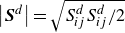 $\left | \boldsymbol{S}^{d} \right |=\sqrt {S_{ij}^{d}S_{ij}^{d}/2}$
, where
$\left | \boldsymbol{S}^{d} \right |=\sqrt {S_{ij}^{d}S_{ij}^{d}/2}$
, where $d$
denotes the deviatoric part of the tensor, i.e.
$d$
denotes the deviatoric part of the tensor, i.e. $\boldsymbol{S}^{d} = \boldsymbol{S} - tr(\boldsymbol{S})\ \boldsymbol{I}/3$
. At
$\boldsymbol{S}^{d} = \boldsymbol{S} - tr(\boldsymbol{S})\ \boldsymbol{I}/3$
. At $t=0$
,
$t=0$
, $\mu _P$
is set to
$\mu _P$
is set to $\mu _P(t=0) = 1$
. The dimensionless consistency parameter
$\mu _P(t=0) = 1$
. The dimensionless consistency parameter $K_c$
is computed using
$K_c$
is computed using $K_c=K {\sigma _{g-m}}^{n-1}a^{-n+1}{\mu _m}^{-n}$
, where
$K_c=K {\sigma _{g-m}}^{n-1}a^{-n+1}{\mu _m}^{-n}$
, where $K$
is the dimensional consistency parameter given by
$K$
is the dimensional consistency parameter given by $\mu _{pol}=\tau _y a/u_c+K(a/u_c)^{n-1}$
, with
$\mu _{pol}=\tau _y a/u_c+K(a/u_c)^{n-1}$
, with $u_c=\mu _m/\sigma _{g-m}$
standing for the characteristic velocity and
$u_c=\mu _m/\sigma _{g-m}$
standing for the characteristic velocity and $\tau _y$
being the yield stress. As the shear rate increases, the polymer viscosity ratio
$\tau _y$
being the yield stress. As the shear rate increases, the polymer viscosity ratio $\mu _P$
decreases following a power-law trend that steepens upon an increase of
$\mu _P$
decreases following a power-law trend that steepens upon an increase of $n$
. When the shear rate tends to the yield stress (hence, when the normalised shear rate tends to
$n$
. When the shear rate tends to the yield stress (hence, when the normalised shear rate tends to $Bi$
), the viscosity of the polymer tends to infinity.
$Bi$
), the viscosity of the polymer tends to infinity.
Several independent non-dimensional groups arise from the momentum equation (2.1b
): the Laplace number ${La}$
, the Weissenberg number
${La}$
, the Weissenberg number ${Wi}$
, the Bingham number
${Wi}$
, the Bingham number ${Bi}$
, the gas-to-liquid density ratio
${Bi}$
, the gas-to-liquid density ratio $\rho$
, the gas-to-mucus dynamic viscosity ratio
$\rho$
, the gas-to-mucus dynamic viscosity ratio $\mu _{g-m}$
, the serous-to-mucus dynamic viscosity ratio
$\mu _{g-m}$
, the serous-to-mucus dynamic viscosity ratio $\mu _{s-m}$
and the reference solvent-to-total dynamic viscosity ratio in the mucus film
$\mu _{s-m}$
and the reference solvent-to-total dynamic viscosity ratio in the mucus film $\mu _S$
. In addition, three additional aspect ratios are required to completely define the problem parameters: the length-to-radius aspect ratio
$\mu _S$
. In addition, three additional aspect ratios are required to completely define the problem parameters: the length-to-radius aspect ratio $\lambda$
, the non-dimensional average serous layer thickness
$\lambda$
, the non-dimensional average serous layer thickness $\epsilon _s$
and the non-dimensional average mucus layer thickness
$\epsilon _s$
and the non-dimensional average mucus layer thickness $\epsilon _m$
. The non-dimensional parameters can be summarised as follows:
$\epsilon _m$
. The non-dimensional parameters can be summarised as follows: $\begin{eqnarray} \begin{array}{cc} {La}=\cfrac {\rho _L \sigma _{g-m} a}{\mu ^2_m}, \quad {Wi}=\cfrac { \sigma _{g-m} (1-\mu _S)}{a G}, \quad {Bi}=\cfrac {\tau _y a}{\sigma _{g-m}}, \quad \mu _S=\cfrac {\mu _{sol}}{\mu _m},\quad \\ \mu _{g-m}=\cfrac {\mu _{G}}{\mu _m}, \,\,\, \mu _{s-m}=\cfrac {\mu _{s}}{\mu _m}, \,\,\, \varSigma _{s-m}=\cfrac {\sigma _{s-m}}{\sigma _{g-m}}, \,\,\, \Delta p=\cfrac {a\left [p(z=0) - p(z=\lambda )\right ]}{\sigma _{g-m}}, \\ \epsilon _s=\cfrac {h_s}{a}, \quad \epsilon _m=\cfrac {h_m}{a}, \quad \epsilon =\cfrac {h}{a}, \quad L_p =\cfrac {l_p}{a}, \quad \lambda =\cfrac {L}{a}, \quad \rho =\cfrac {\rho _G}{\rho _L}, \quad \end{array} \end{eqnarray}$
where $G$
is the elastic modulus, the serous and mucus have the same density
$G$
is the elastic modulus, the serous and mucus have the same density $\rho _s=\rho _m=\rho _L$
, and the reference relaxation time is calculated as
$\rho _s=\rho _m=\rho _L$
, and the reference relaxation time is calculated as $\varLambda _r=\mu _{pol}/G$
.
$\varLambda _r=\mu _{pol}/G$
.
Finally, to mimic inhaling conditions, a constant pressure difference $\Delta p = p(z=0) - p(z=\lambda )\gt 0$
between the left and right ends of the airway is enforced to drive movement of the liquid plug. At
$\Delta p = p(z=0) - p(z=\lambda )\gt 0$
between the left and right ends of the airway is enforced to drive movement of the liquid plug. At $t=0$
, the left and right total film thicknesses are fixed to
$t=0$
, the left and right total film thicknesses are fixed to $\epsilon$
, and the capillary pressure jumps
$\epsilon$
, and the capillary pressure jumps $[\![p]\!]_{g-m}$
and
$[\![p]\!]_{g-m}$
and $[\![p]\!]_{s-m}$
across the gas–mucus interface and serous–mucus interface, respectively, are included as
$[\![p]\!]_{s-m}$
across the gas–mucus interface and serous–mucus interface, respectively, are included as $[\![p]\!]_{g-m}=(1-\epsilon )^{-1}$
and
$[\![p]\!]_{g-m}=(1-\epsilon )^{-1}$
and $[\![p]\!]_{s-m}=\varSigma _{s-m}(1-\epsilon _s)^{-1}$
because we use a capillary scaling:
$[\![p]\!]_{s-m}=\varSigma _{s-m}(1-\epsilon _s)^{-1}$
because we use a capillary scaling: $\begin{aligned} p(z=0) = \left \{ \begin{array}{l}\! \Delta p \\ \Delta p-[\![p]\!]_{g-m} \\ \Delta p-[\![p]\!]_{g-m}-[\![p]\!]_{s-m} \end{array} \right., \quad p(z=\lambda ) = \left \{ \begin{array}{ll} 0 & \mathrm{air\ core} \\ -[\![p]\!]_{g-m} & \mathrm{mucus\ layer} \\ -[\![p]\!]_{g-m}-[\![p]\!]_{s-m} & \mathrm{serous\ layer} \end{array} \right. . \end{aligned}$
The mathematical problem (2.1) is closed by enforcing uniformly homogeneous Neumann conditions for velocity at the inlet and outlet, i.e. at $z=0$
and
$z=0$
and $z=\lambda$
. The tangential stress magnitudes and corresponding tangential velocities are matched across the air–mucus and mucus–serous interfaces, ensuring continuity in each phase. No-slip and no-penetration conditions are enforced along the wall, i.e. at
$z=\lambda$
. The tangential stress magnitudes and corresponding tangential velocities are matched across the air–mucus and mucus–serous interfaces, ensuring continuity in each phase. No-slip and no-penetration conditions are enforced along the wall, i.e. at $r=1$
, while axisymmetric conditions are set at
$r=1$
, while axisymmetric conditions are set at $r=0$
.
$r=0$
.
2.2. Physiological parameters
This study aims to model the propagation and rupture of liquid plugs using a two-layer model, considering the elastoviscoplastic properties of mucus. We emphasise the physiological significance of formulating the non-dimensional parameter space in terms of dimensional quantities within the range of health and pathology. Since plug propagation and rupture are predominantly governed by surface tension-driven dynamics, the Laplace number emerges as a critical determinant (Fujioka et al. Reference Fujioka, Takayama and Grotberg2008; Hassan et al. Reference Hassan, Uzgoren, Fujioka, Grotberg and Shyy2011; Muradoglu et al. Reference Muradoglu, Romanò, Fujioka and Grotberg2019). Hence, varying ${La}$
enables incorporation of the full spectrum of physiologically relevant parameters. In accordance with Guidotti (Reference Guidotti1997), we adopt an airway radius of
${La}$
enables incorporation of the full spectrum of physiologically relevant parameters. In accordance with Guidotti (Reference Guidotti1997), we adopt an airway radius of $a\in [0.65, 1.2 ]$
mm as representative of the typical dimensions found in the eighth-to-tenth generation of adult lung airways where surface tension dominates and gravity is negligible (Romanò et al. Reference Romanò, Muradoglu and Grotberg2022). The dimensionless initial plug length is set to
$a\in [0.65, 1.2 ]$
mm as representative of the typical dimensions found in the eighth-to-tenth generation of adult lung airways where surface tension dominates and gravity is negligible (Romanò et al. Reference Romanò, Muradoglu and Grotberg2022). The dimensionless initial plug length is set to $L_p(t=0)=1$
, while the non-dimensional centre of the plug is initially set at
$L_p(t=0)=1$
, while the non-dimensional centre of the plug is initially set at $z_p(t=0)=2.95$
and the length-to-radius ratio
$z_p(t=0)=2.95$
and the length-to-radius ratio $\lambda$
of the airway is extended to 16 to reduce the influence of inflow and outflow conditions. In healthy conditions (Guo & Kanso Reference Guo and Kanso2017), the serous layer thickness generally is
$\lambda$
of the airway is extended to 16 to reduce the influence of inflow and outflow conditions. In healthy conditions (Guo & Kanso Reference Guo and Kanso2017), the serous layer thickness generally is $h_s \approx [40\,\%,80\,\%]h_{cilia}$
, where
$h_s \approx [40\,\%,80\,\%]h_{cilia}$
, where $h_{cilia}$
is cilia length, while the total airway surface liquid thickness is
$h_{cilia}$
is cilia length, while the total airway surface liquid thickness is $h_m+h_s \approx 2h_{cilia}$
. Therefore, the mucus-to-serous layer thickness ratio is taken as 3 for the baseline case. In healthy to pathological conditions, the alterations in airway surface liquid secretion lead to a total fluid film thickness (
$h_m+h_s \approx 2h_{cilia}$
. Therefore, the mucus-to-serous layer thickness ratio is taken as 3 for the baseline case. In healthy to pathological conditions, the alterations in airway surface liquid secretion lead to a total fluid film thickness ( $\epsilon =\epsilon _s+\epsilon _m$
) ranging from approximately 0.03 to 0.3 (hyper-secretion of mucus, Sackner & Kim Reference Sackner and Kim1987; Yager et al. Reference Yager, Cloutier, Feldman, Bastacky, Drazen and Kamm1994; Fujioka et al. Reference Fujioka, Takayama and Grotberg2008; Fahy & Dickey Reference Fahy and Dickey2010). As recommended by Hassan et al. (Reference Hassan, Uzgoren, Fujioka, Grotberg and Shyy2011) and Muradoglu et al. (Reference Muradoglu, Romanò, Fujioka and Grotberg2019), the initial dimensionless total film thickness
$\epsilon =\epsilon _s+\epsilon _m$
) ranging from approximately 0.03 to 0.3 (hyper-secretion of mucus, Sackner & Kim Reference Sackner and Kim1987; Yager et al. Reference Yager, Cloutier, Feldman, Bastacky, Drazen and Kamm1994; Fujioka et al. Reference Fujioka, Takayama and Grotberg2008; Fahy & Dickey Reference Fahy and Dickey2010). As recommended by Hassan et al. (Reference Hassan, Uzgoren, Fujioka, Grotberg and Shyy2011) and Muradoglu et al. (Reference Muradoglu, Romanò, Fujioka and Grotberg2019), the initial dimensionless total film thickness $\epsilon$
ranges from 0.03 to 0.07 for both the trailing film and front film. Following Romanò et al. (Reference Romanò, Fujioka, Muradoglu and Grotberg2019) and Erken et al. (Reference Erken, Fazla, Muradoglu, Izbassarov, Romanò and Grotberg2023), the multilayer liquid’s density, comprising mucus and serous components, closely matches that of water (
$\epsilon$
ranges from 0.03 to 0.07 for both the trailing film and front film. Following Romanò et al. (Reference Romanò, Fujioka, Muradoglu and Grotberg2019) and Erken et al. (Reference Erken, Fazla, Muradoglu, Izbassarov, Romanò and Grotberg2023), the multilayer liquid’s density, comprising mucus and serous components, closely matches that of water ( $\rho _m=\rho _s=1$ $\text{g cm}^{-3}$
), resulting in a gas-to-liquid density ratio of
$\text{g cm}^{-3}$
), resulting in a gas-to-liquid density ratio of $\rho =10^{-3}$
. The serous layer exhibits a dynamic viscosity similar to water,
$\rho =10^{-3}$
. The serous layer exhibits a dynamic viscosity similar to water, $\mu _s \approx$
0.01 poise. Meanwhile, the dynamic viscosity of mucus (
$\mu _s \approx$
0.01 poise. Meanwhile, the dynamic viscosity of mucus ( $ \mu _m$
) layer can span across several orders of magnitude (Lai et al. Reference Lai, Wang, Wirtz and Hanes2009; Fahy & Dickey Reference Fahy and Dickey2010; Romanò et al. Reference Romanò, Fujioka, Muradoglu and Grotberg2019; Patarin et al. Reference Patarin, Ghiringhelli, Darsy, Obamba, Bochu, Camara, Quétant, Cracowski, Cracowski and Robert de Saint Vincent2020; Erken et al. Reference Erken, Fazla, Muradoglu, Izbassarov, Romanò and Grotberg2023). So, the serous-to-mucus dynamic viscosity ratio
$ \mu _m$
) layer can span across several orders of magnitude (Lai et al. Reference Lai, Wang, Wirtz and Hanes2009; Fahy & Dickey Reference Fahy and Dickey2010; Romanò et al. Reference Romanò, Fujioka, Muradoglu and Grotberg2019; Patarin et al. Reference Patarin, Ghiringhelli, Darsy, Obamba, Bochu, Camara, Quétant, Cracowski, Cracowski and Robert de Saint Vincent2020; Erken et al. Reference Erken, Fazla, Muradoglu, Izbassarov, Romanò and Grotberg2023). So, the serous-to-mucus dynamic viscosity ratio $\mu _{s-m}$
ranges from 0.01 to 0.4. Romanò et al. (Reference Romanò, Fujioka, Muradoglu and Grotberg2019) demonstrated that variations in the gas-to-mucus viscosity ratio exert only a marginal influence on wall shear stresses. Consequently, as the present investigation centres on the influence of the serous layer on wall stress distributions, the gas-to-mucus dynamic viscosity ratio is held constant at
$\mu _{s-m}$
ranges from 0.01 to 0.4. Romanò et al. (Reference Romanò, Fujioka, Muradoglu and Grotberg2019) demonstrated that variations in the gas-to-mucus viscosity ratio exert only a marginal influence on wall shear stresses. Consequently, as the present investigation centres on the influence of the serous layer on wall stress distributions, the gas-to-mucus dynamic viscosity ratio is held constant at $\mu _{g-m}=1.5\times 10^{-3}$
throughout all simulations reported herein, additionally, where dynamic viscosity of air at
$\mu _{g-m}=1.5\times 10^{-3}$
throughout all simulations reported herein, additionally, where dynamic viscosity of air at $37\,^\circ\text{C}$
(
$37\,^\circ\text{C}$
( $ \mu _G = 1.89 \times 10^{-4}$
poise) is considered. The interfacial tension at the air–mucus interface was prescribed as
$ \mu _G = 1.89 \times 10^{-4}$
poise) is considered. The interfacial tension at the air–mucus interface was prescribed as $\sigma _{g-m} \approx 0.0244$
N m−1, reported by Tai et al. (Reference Tai, Bian, Halpern, Zheng, Filoche and Grotberg2011), Romanò et al. (Reference Romanò, Fujioka, Muradoglu and Grotberg2019) and Muradoglu et al. (Reference Muradoglu, Romanò, Fujioka and Grotberg2019). To the best of our knowledge, no prior studies have quantified the interfacial surface tension between the mucus and serous layers. Based on two liquid films of the same aqueous material, a baseline value of
$\sigma _{g-m} \approx 0.0244$
N m−1, reported by Tai et al. (Reference Tai, Bian, Halpern, Zheng, Filoche and Grotberg2011), Romanò et al. (Reference Romanò, Fujioka, Muradoglu and Grotberg2019) and Muradoglu et al. (Reference Muradoglu, Romanò, Fujioka and Grotberg2019). To the best of our knowledge, no prior studies have quantified the interfacial surface tension between the mucus and serous layers. Based on two liquid films of the same aqueous material, a baseline value of $\varSigma _{s-m}=0.1$
is adopted in this study. However, we also perform a sensitivity investigation to make sure that our model predictions do not get affected by such an assumption in Appendix B.
$\varSigma _{s-m}=0.1$
is adopted in this study. However, we also perform a sensitivity investigation to make sure that our model predictions do not get affected by such an assumption in Appendix B.
The serous layer is commonly modelled as a Newtonian liquid (Tarran et al. Reference Tarran, Grubb, Parsons, Picher, Hirsh, Davis and Boucher2001; Boucher Reference Boucher2004; Button et al. Reference Button, Cai, Ehre, Kesimer, Hill, Sheehan, Boucher and Rubinstein2012; Guo & Kanso Reference Guo and Kanso2017). The relaxation time of elastoviscoplastic mucus can range from 0.002 to 2 s, corresponding to characteristic Weissenberg numbers ( ${Wi}$
) ranging from 10 to 1000, which covers all healthy and diseased conditions accounted for in the previous studies (Patarin et al. Reference Patarin, Ghiringhelli, Darsy, Obamba, Bochu, Camara, Quétant, Cracowski, Cracowski and Robert de Saint Vincent2020; Romanò et al. Reference Romanò, Muradoglu, Fujioka and Grotberg2021; Choudhury et al. Reference Choudhury, Filoche, Ribe, Grenier and Dietze2023; Erken et al. Reference Erken, Fazla, Muradoglu, Izbassarov, Romanò and Grotberg2023; Hao et al. Reference Hao, Izbassarov, Muradoglu, Grotberg, Lacassagne, Bahrani and Romanò2025). In addition,
${Wi}$
) ranging from 10 to 1000, which covers all healthy and diseased conditions accounted for in the previous studies (Patarin et al. Reference Patarin, Ghiringhelli, Darsy, Obamba, Bochu, Camara, Quétant, Cracowski, Cracowski and Robert de Saint Vincent2020; Romanò et al. Reference Romanò, Muradoglu, Fujioka and Grotberg2021; Choudhury et al. Reference Choudhury, Filoche, Ribe, Grenier and Dietze2023; Erken et al. Reference Erken, Fazla, Muradoglu, Izbassarov, Romanò and Grotberg2023; Hao et al. Reference Hao, Izbassarov, Muradoglu, Grotberg, Lacassagne, Bahrani and Romanò2025). In addition, $0.001 \leqslant {Bi} \leqslant 0.1$
and
$0.001 \leqslant {Bi} \leqslant 0.1$
and $0.3 \leqslant n \leqslant 1$
are defined respectively in accordance with studies of Erken et al. (Reference Erken, Fazla, Muradoglu, Izbassarov, Romanò and Grotberg2023) and Hao et al. (Reference Hao, Izbassarov, Muradoglu, Grotberg, Lacassagne, Bahrani and Romanò2025), to encompass a broad spectrum of physiological scenarios. Thus, the baseline case is defined as
$0.3 \leqslant n \leqslant 1$
are defined respectively in accordance with studies of Erken et al. (Reference Erken, Fazla, Muradoglu, Izbassarov, Romanò and Grotberg2023) and Hao et al. (Reference Hao, Izbassarov, Muradoglu, Grotberg, Lacassagne, Bahrani and Romanò2025), to encompass a broad spectrum of physiological scenarios. Thus, the baseline case is defined as ${La}=100$
,
${La}=100$
, $\Delta p=2$
,
$\Delta p=2$
, $\epsilon _s=0.015$
,
$\epsilon _s=0.015$
, $\epsilon =0.05$
,
$\epsilon =0.05$
, $\mu _{s-m}=0.08$
,
$\mu _{s-m}=0.08$
, $\varSigma _{s-m}=0.1$
,
$\varSigma _{s-m}=0.1$
, ${Wi}=0$
,
${Wi}=0$
, ${Bi}=0$
,
${Bi}=0$
, $n=1$
,
$n=1$
, $\mu _{g-m}=1.5\times 10^{-3}$
and
$\mu _{g-m}=1.5\times 10^{-3}$
and $\lambda =16$
. The non-dimensional parameters employed in the present investigation are summarised in table 1. We explore a parametric space that accounts for all the combinations of relevant parameters, without having to hypothesise for specific correlations. On the one hand, this implied more simulations than physiologically needed, but on the other hand, it allowed us to test the robustness of physical mechanism even beyond the strict scope of our model.
$\lambda =16$
. The non-dimensional parameters employed in the present investigation are summarised in table 1. We explore a parametric space that accounts for all the combinations of relevant parameters, without having to hypothesise for specific correlations. On the one hand, this implied more simulations than physiologically needed, but on the other hand, it allowed us to test the robustness of physical mechanism even beyond the strict scope of our model.
Ranges of the non-dimensional parameters used in the simulations.

3. Numerical method
The airway reopening phenomenon is modelled in an axisymmetric domain, with the enforcement of azimuthal derivative $\partial _{\phi }=0$
and azimuthal velocity
$\partial _{\phi }=0$
and azimuthal velocity $u_{\phi }=0$
. Integrating the governing equations (2.1) over time is achieved through a fractional step method employing a second-order pressure-correction projection scheme. Implicit treatment is applied to the viscous term, while explicit discretisation is employed for the nonlinear convective term using the Bell–Collela–Glaz advection scheme (Bell, Colella & Glaz Reference Bell, Colella and Glaz1989).
$u_{\phi }=0$
. Integrating the governing equations (2.1) over time is achieved through a fractional step method employing a second-order pressure-correction projection scheme. Implicit treatment is applied to the viscous term, while explicit discretisation is employed for the nonlinear convective term using the Bell–Collela–Glaz advection scheme (Bell, Colella & Glaz Reference Bell, Colella and Glaz1989).
To simulate this three-phase problem, we employ an extended conventional two-phase volume-of-fluid (VOF) method to accommodate three distinct interfaces. Specifically, we use three volume fraction fields, denoted as $f_g(r,z,t)$
,
$f_g(r,z,t)$
, $f_m(r,z,t)$
and
$f_m(r,z,t)$
and $f_s(r,z,t)$
, corresponding to the air, mucus and serous phases, respectively. Each volume fraction is defined to be unity within its respective phase and zero elsewhere. This formulation enables the use of a unified one-fluid approach analogous for the mixture properties such as density
$f_s(r,z,t)$
, corresponding to the air, mucus and serous phases, respectively. Each volume fraction is defined to be unity within its respective phase and zero elsewhere. This formulation enables the use of a unified one-fluid approach analogous for the mixture properties such as density $\tilde {\rho }$
, viscosity
$\tilde {\rho }$
, viscosity $\tilde {\mu }$
and elastic modulus
$\tilde {\mu }$
and elastic modulus $\tilde {G}$
are computed as arithmetic averages based on the local volume fractions:
$\tilde {G}$
are computed as arithmetic averages based on the local volume fractions: $\begin{equation} \tilde {\rho }(f)=f_g\rho _g+f_m\rho _m+f_s\rho _s, \quad \tilde {\mu }(f)=f_g{\mu }_g+f_m{\mu }_m+f_s{\mu }_s, \quad \tilde {G}(f)=f_m{G} . \end{equation}$
The advection equation governing the volume fraction in multiphase flow models the transport of individual phases within a multi-phase mixture. It is formulated by considering polyphase control volumes composed of multiple immiscible phases, each characterised by a distinct volume fraction representing its local spatial occupancy: $\begin{equation} \partial _tf_j+\boldsymbol{\nabla }\boldsymbol{\cdot }(f_j\boldsymbol{u})=0, \end{equation}$
where $j$
refers to
$j$
refers to $g$
,
$g$
, $m$
and
$m$
and $s$
, respectively. The piecewise linear interface construction (PLIC) method is employed to reconstruct the interface. The interface normal vector is determined using the mixed-Youngs-centred (MYC) scheme, as described by Aulisa, Manservisi & Scardovelli (Reference Aulisa, Manservisi and Scardovelli2006), while the interface position within each cell is computed following the approach proposed by Scardovelli & Zaleski (Reference Scardovelli and Zaleski2000). Following Popinet (Reference Popinet2009), surface tension is treated using a combination of the balanced-force formulation and a height-function-based curvature estimator. This approach significantly reduces numerical artefacts associated with the discretisation of
$s$
, respectively. The piecewise linear interface construction (PLIC) method is employed to reconstruct the interface. The interface normal vector is determined using the mixed-Youngs-centred (MYC) scheme, as described by Aulisa, Manservisi & Scardovelli (Reference Aulisa, Manservisi and Scardovelli2006), while the interface position within each cell is computed following the approach proposed by Scardovelli & Zaleski (Reference Scardovelli and Zaleski2000). Following Popinet (Reference Popinet2009), surface tension is treated using a combination of the balanced-force formulation and a height-function-based curvature estimator. This approach significantly reduces numerical artefacts associated with the discretisation of $\chi \boldsymbol{n} \delta _s$
, enabling second-order convergence.
$\chi \boldsymbol{n} \delta _s$
, enabling second-order convergence.
The pronounced elasticity of the non-Newtonian fluid renders the numerical solution of the constitutive equation difficult to integrate in time (Fattal & Kupferman Reference Fattal and Kupferman2004, Reference Fattal and Kupferman2005), due to the elevated Weissenberg numbers characterising pulmonary flows. The flow is supposed, in fact, to embed regions of high stress and fine features, which are known to induce numerical instabilities. This potential instability imposes practical constraints on the values of the relaxation time of the elastoviscoplastic fluid $\varLambda _r$
. To surmount this challenge, (2.3) is recasted using the log-conformation representation proposed by Fattal & Kupferman (Reference Fattal and Kupferman2004, Reference Fattal and Kupferman2005).
$\varLambda _r$
. To surmount this challenge, (2.3) is recasted using the log-conformation representation proposed by Fattal & Kupferman (Reference Fattal and Kupferman2004, Reference Fattal and Kupferman2005).
The spatial and temporal discretisations are implemented using the open-source simulation framework Basilisk (Popinet & Collaborators Reference Popinet2013–2015; López-Herrera et al. Reference López-Herrera, Popinet and Castrejón-Pita2019), which has been extensively validated through a wide range of benchmark problems. Given that our study focuses on thin film dynamics and the associated wall stresses, we optimise computational efficiency by employing an adaptive mesh refinement (AMR) strategy basing on a quadtree grid. By using the ’mask’ function in Basilisk to exclude the computational domain where $r \gt 1$
, the top wall boundary is implemented. Basilisk has demonstrated robustness and accuracy across various multiphase flow applications of practical relevance. Specifically, the same code has been rigorously applied to problems involving airway closure (Romanò et al. Reference Romanò, Fujioka, Muradoglu and Grotberg2019, Reference Romanò, Muradoglu, Fujioka and Grotberg2021) and airway reopening (Hao et al. Reference Hao, Izbassarov, Muradoglu, Grotberg, Lacassagne, Bahrani and Romanò2025), where AMR is also used. In the present work, we extend this validation to the context of three phases. In Appendix A, the results of Basilisk are compared with those of the front-tracking method reported by Erken et al. (Reference Erken, Romano, Grotberg and Muradoglu2022), demonstrating good agreement. Subsequently, a grid independence study is established.
$r \gt 1$
, the top wall boundary is implemented. Basilisk has demonstrated robustness and accuracy across various multiphase flow applications of practical relevance. Specifically, the same code has been rigorously applied to problems involving airway closure (Romanò et al. Reference Romanò, Fujioka, Muradoglu and Grotberg2019, Reference Romanò, Muradoglu, Fujioka and Grotberg2021) and airway reopening (Hao et al. Reference Hao, Izbassarov, Muradoglu, Grotberg, Lacassagne, Bahrani and Romanò2025), where AMR is also used. In the present work, we extend this validation to the context of three phases. In Appendix A, the results of Basilisk are compared with those of the front-tracking method reported by Erken et al. (Reference Erken, Romano, Grotberg and Muradoglu2022), demonstrating good agreement. Subsequently, a grid independence study is established.
4. Results and discussion
Given the complex rheological behaviour of the mucus layer and its interactions with adjacent serous layers, we first model the mucus as Newtonian, then include viscoelasticity and finally we consider elastoviscoplasticity. The goal is to enable a systematic analysis of the influence of each rheological feature. A baseline analysis of two-layer airway reopening with Newtonian fluids is presented in § 4.1 and a subsequent parametric study for Newtonian mucus is presented in §§ 4.2–4.4, where the complex fluid dimensionless parameters are set to ${Wi}=0$
,
${Wi}=0$
, ${Bi}=0$
and
${Bi}=0$
and $n=1$
thereby switching from the Saramito–HB solver to the Newtonian solver directly. The necessity of the two-layer model is explained in § 4.5. Sections 4.6 and 4.7 examine the influence of different rheological behaviours. Specifically, we evaluate viscoelasticity using an Oldroyd-B model (
$n=1$
thereby switching from the Saramito–HB solver to the Newtonian solver directly. The necessity of the two-layer model is explained in § 4.5. Sections 4.6 and 4.7 examine the influence of different rheological behaviours. Specifically, we evaluate viscoelasticity using an Oldroyd-B model ( ${Bi}=0, n=1$
), viscoplasticity by varying
${Bi}=0, n=1$
), viscoplasticity by varying ${Bi}$
and
${Bi}$
and $n$
at a fixed
$n$
at a fixed ${Wi}=10$
, and elastoviscoplasticity via the comprehensive Saramito–HB model. Finally, in § 4.8, we discussed the effects of all parameters on critical plug length.
${Wi}=10$
, and elastoviscoplasticity via the comprehensive Saramito–HB model. Finally, in § 4.8, we discussed the effects of all parameters on critical plug length.
4.1. Analysis of a typical Newtonian two-layer airway reopening scenario
Figure 2(a–c) shows evolution of the interface (solid magenta line, air–mucus interface; solid orange line, mucus–serous interface) with contours of the pressure field, alongside the axial velocity profiles depicted at a distance of airway radius for the baseline case at three instants of time ( $t=18, 42, 60$
). Figure 2(d–e) is the enlarged views of the cyan box in figure 2(b–c), respectively. In all snapshots, the pressure field inside the plug bulk exhibits qualitative consistency with the one-layer rupture reported by Hassan et al. (Reference Hassan, Uzgoren, Fujioka, Grotberg and Shyy2011), Muradoglu et al. (Reference Muradoglu, Romanò, Fujioka and Grotberg2019) and Hao et al. (Reference Hao, Izbassarov, Muradoglu, Grotberg, Lacassagne, Bahrani and Romanò2025). The pressure within the plug exhibits a gradual decline along the flow direction, reaching its minimum at the front meniscus, where location corresponds to the region of minimum liquid film thickness. The liquid flow through the constricted region of the film induces a highly localised pressure drop. In response, the interface is drawn towards this low-pressure zone, resulting in a pronounced increase in interfacial curvature to balance the enhanced pressure differential across the phase boundary. As shown in figure 2(d–e), the mucus–serous interface also deforms along with the air–mucus interface to compensate for the localised significant pressure drop. Moreover, a backflow is observed ahead of the leading air finger, associated with the local pressure minimum, as also reported by Hassan et al. (Reference Hassan, Uzgoren, Fujioka, Grotberg and Shyy2011), Muradoglu et al. (Reference Muradoglu, Romanò, Fujioka and Grotberg2019) and Hao et al. (Reference Hao, Izbassarov, Muradoglu, Grotberg, Lacassagne, Bahrani and Romanò2025). The velocity consistently exhibits its highest magnitude near the centreline and increases progressively throughout the propagation. In regions distal to the plug, the velocity of the liquid film is significantly lower than the average velocity of the advancing air finger, suggesting that the far-field liquid film exhibits negligible propagation in conjunction with the plug. In contrast, the liquid plug itself moves at a substantially higher velocity than that of the surrounding liquid film, while still remaining slower than the air finger. This kinematic behaviour implies that the plug undergoes continuous liquid deposition throughout its propagation. When the deposited liquid exceeds the pre-wetted coating, the plug diminishes in size and may ultimately rupture.
$t=18, 42, 60$
). Figure 2(d–e) is the enlarged views of the cyan box in figure 2(b–c), respectively. In all snapshots, the pressure field inside the plug bulk exhibits qualitative consistency with the one-layer rupture reported by Hassan et al. (Reference Hassan, Uzgoren, Fujioka, Grotberg and Shyy2011), Muradoglu et al. (Reference Muradoglu, Romanò, Fujioka and Grotberg2019) and Hao et al. (Reference Hao, Izbassarov, Muradoglu, Grotberg, Lacassagne, Bahrani and Romanò2025). The pressure within the plug exhibits a gradual decline along the flow direction, reaching its minimum at the front meniscus, where location corresponds to the region of minimum liquid film thickness. The liquid flow through the constricted region of the film induces a highly localised pressure drop. In response, the interface is drawn towards this low-pressure zone, resulting in a pronounced increase in interfacial curvature to balance the enhanced pressure differential across the phase boundary. As shown in figure 2(d–e), the mucus–serous interface also deforms along with the air–mucus interface to compensate for the localised significant pressure drop. Moreover, a backflow is observed ahead of the leading air finger, associated with the local pressure minimum, as also reported by Hassan et al. (Reference Hassan, Uzgoren, Fujioka, Grotberg and Shyy2011), Muradoglu et al. (Reference Muradoglu, Romanò, Fujioka and Grotberg2019) and Hao et al. (Reference Hao, Izbassarov, Muradoglu, Grotberg, Lacassagne, Bahrani and Romanò2025). The velocity consistently exhibits its highest magnitude near the centreline and increases progressively throughout the propagation. In regions distal to the plug, the velocity of the liquid film is significantly lower than the average velocity of the advancing air finger, suggesting that the far-field liquid film exhibits negligible propagation in conjunction with the plug. In contrast, the liquid plug itself moves at a substantially higher velocity than that of the surrounding liquid film, while still remaining slower than the air finger. This kinematic behaviour implies that the plug undergoes continuous liquid deposition throughout its propagation. When the deposited liquid exceeds the pre-wetted coating, the plug diminishes in size and may ultimately rupture.
(a–c) Evolution of the interface (solid magenta line, air–mucus interface; solid orange line, mucus–serous interface) with contours of the pressure field and the velocity vectors for the baseline case. (d) Enlarged views of the front meniscus of the liquid plug (d) for panel (b) and (e) for panel (c). ( ${La}=100$
,
${La}=100$
, $\Delta p=2$
,
$\Delta p=2$
, $\epsilon _s=0.015$
,
$\epsilon _s=0.015$
, $\epsilon =0.05$
,
$\epsilon =0.05$
, $\mu _{s-m}=0.08$
,
$\mu _{s-m}=0.08$
, $\varSigma _{s-m}=0.1$
,
$\varSigma _{s-m}=0.1$
, ${Wi}=0$
,
${Wi}=0$
, ${Bi}=0$
,
${Bi}=0$
, $n=1$
,
$n=1$
, $\mu _{g-m}=1.5\times 10^{-3}$
and
$\mu _{g-m}=1.5\times 10^{-3}$
and $\lambda =16$
.)
$\lambda =16$
.)

Figure 2. Long description
The image contains five panels showing the evolution of the interface within a liquid plug in an airway. Panels (a), (b), and (c) display the interface at different time points (t = 18, t = 42, t = 60) with solid magenta and orange lines representing the airmucus and mucusserous interfaces, respectively. These panels include contours of the pressure field and velocity vectors, illustrating the dynamics of the liquid plug. Panels (d) and (e) provide enlarged views of the front meniscus of the liquid plug for time points t = 42 and t = 60, respectively. The velocity vectors indicate the direction and magnitude of fluid movement, while the color gradient represents the pressure field, ranging from -4 to 2. The graphs collectively show how the liquid plug evolves over time, influenced by pressure gradients and velocity fields.
Figure 3 shows a comparison between the two-layer plug propagation (solid line) and the one-layer plug propagation (dashed line) at two instants ( $t=10$
and
$t=10$
and $t=45$
), characterised by the interface (figure 3
a), the wall pressure
$t=45$
), characterised by the interface (figure 3
a), the wall pressure $p_w$
(figure 3
b) and the wall shear stress
$p_w$
(figure 3
b) and the wall shear stress $\tau _w$
(figure 3
c). At the initial stage (
$\tau _w$
(figure 3
c). At the initial stage ( $t = 10$
, blue curve), the two plugs propagate in close proximity, with the two-layer plug slightly ahead of the one-layer plug, as shown in figure 3(a). The magnified view (cyan inset) reveals a wrinkled serous–mucus interface near the the front plug meniscus, attributed to capillary wave propagation along the mucus–air interface. As illustrated in figure 3(b), the distribution of
$t = 10$
, blue curve), the two plugs propagate in close proximity, with the two-layer plug slightly ahead of the one-layer plug, as shown in figure 3(a). The magnified view (cyan inset) reveals a wrinkled serous–mucus interface near the the front plug meniscus, attributed to capillary wave propagation along the mucus–air interface. As illustrated in figure 3(b), the distribution of $p_w$
exhibits qualitatively similar trends for both cases, with the minimum pressure consistently located at the front plug meniscus. For the two-layer case,
$p_w$
exhibits qualitatively similar trends for both cases, with the minimum pressure consistently located at the front plug meniscus. For the two-layer case, $\mathrm{max}{(p_w)}$
is smaller than for the one-layer case, which may be attributed to the presence of wrinkled interfaces, which partially relieve the capillary pressure projected from the air–mucus interface. The distributions of
$\mathrm{max}{(p_w)}$
is smaller than for the one-layer case, which may be attributed to the presence of wrinkled interfaces, which partially relieve the capillary pressure projected from the air–mucus interface. The distributions of $\tau _w$
for the two cases do not exhibit significant qualitative differences, as shown in figure 3(c), i.e. during plug propagation,
$\tau _w$
for the two cases do not exhibit significant qualitative differences, as shown in figure 3(c), i.e. during plug propagation, $\mathrm{max}{(\tau _w)}$
consistently localises near the front meniscus, and the thin films located ahead of and behind the plug remain almost unaffected. However, quantitatively, for the two-layer plug,
$\mathrm{max}{(\tau _w)}$
consistently localises near the front meniscus, and the thin films located ahead of and behind the plug remain almost unaffected. However, quantitatively, for the two-layer plug, $\tau _w$
is significantly lower compared with the one-layer plug, and this reduction is particularly pronounced in regions exhibiting sharp stress derivatives, where the stress in the two-layer film decreases by up to
$\tau _w$
is significantly lower compared with the one-layer plug, and this reduction is particularly pronounced in regions exhibiting sharp stress derivatives, where the stress in the two-layer film decreases by up to $75\,\%$
relative to that in the one-layer film. This protective role of the serous layer for the airway is also found in the airway closure (Erken et al. Reference Erken, Romano, Grotberg and Muradoglu2022).
$75\,\%$
relative to that in the one-layer film. This protective role of the serous layer for the airway is also found in the airway closure (Erken et al. Reference Erken, Romano, Grotberg and Muradoglu2022).
For $t=45$
(red lines), as shown in figure 3(a), the two-layer plug propagates a significantly greater distance than the one-layer plug. Consequently, a two-layer plug is less prone to rupture within a finite-length airway, which increases the risk of airway reopening failure. As the plug advances, both
$t=45$
(red lines), as shown in figure 3(a), the two-layer plug propagates a significantly greater distance than the one-layer plug. Consequently, a two-layer plug is less prone to rupture within a finite-length airway, which increases the risk of airway reopening failure. As the plug advances, both $\mathrm{max}(p_w)$
and
$\mathrm{max}(p_w)$
and $\mathrm{max}(\tau _w)$
continue to increase, as shown by red lines in figures 3(b) and 3(c). Moreover, the protective effect of the serous layer is more significant, reducing
$\mathrm{max}(\tau _w)$
continue to increase, as shown by red lines in figures 3(b) and 3(c). Moreover, the protective effect of the serous layer is more significant, reducing $\mathrm{max}(p_w)$
and
$\mathrm{max}(p_w)$
and $\mathrm{max}(\tau _w)$
further.
$\mathrm{max}(\tau _w)$
further.
Comparison of the (a) interface, (b) wall pressure and (c) wall shear stress between the two-layer (solid line) and one-layer (dashed line) models at two instants $t=10$
(blue) and
$t=10$
(blue) and $t=45$
(red). The cyan corner shows an enlarged view of the front meniscus. The parameters of the two-layer case are set as
$t=45$
(red). The cyan corner shows an enlarged view of the front meniscus. The parameters of the two-layer case are set as $\epsilon _s=0.015$
,
$\epsilon _s=0.015$
, $\epsilon =0.05$
,
$\epsilon =0.05$
, $\mu _{s-m}=0.08$
and
$\mu _{s-m}=0.08$
and $\varSigma _{s-m}=0.1$
, while the parameter for the one-layer case are set as
$\varSigma _{s-m}=0.1$
, while the parameter for the one-layer case are set as $\epsilon =0.05$
, with
$\epsilon =0.05$
, with $\epsilon _s=0$
,
$\epsilon _s=0$
, $\mu _{s-m}=1$
and
$\mu _{s-m}=1$
and $\varSigma _{s-m}=0$
. The rest of the parameters are fixed for both cases as
$\varSigma _{s-m}=0$
. The rest of the parameters are fixed for both cases as ${La}=100$
,
${La}=100$
, $\Delta p=2$
,
$\Delta p=2$
, ${Wi}=0$
,
${Wi}=0$
, ${Bi}=0$
,
${Bi}=0$
, $n=1$
,
$n=1$
, $\mu _{g-m}=1.5\times 10^{-3}$
and
$\mu _{g-m}=1.5\times 10^{-3}$
and $\lambda =16$
.
$\lambda =16$
.

Figure 3. Long description
The image contains three line graphs labeled (a), (b), and (c), comparing the interface, wall pressure, and wall shear stress between two-layer (solid lines) and one-layer (dashed lines) models at two different time points, represented by blue and red lines. Graph (a) shows the interface with two insets providing enlarged views of the front meniscus. Graph (b) depicts wall pressure, and graph (c) illustrates wall shear stress. The x-axis represents the spatial coordinate z, while the y-axes represent the interface position r, wall pressure pw, and wall shear stress τw, respectively. The two-layer model parameters are set as epsilon_s = 0.015, epsilon = 0.05, mu_{s-m} = 0.08 and Sigma_{s-m} = 0.1, while the one-layer model parameters are set as epsilon = 0.5, with epsilon_s = 0, mu_{s-m} = 1 and Sigma_{s-m} = 0, and the rest of the parameters are fixed for both cases as La = 100, Delta p = 2, Wi = 0, Bi = 0, n = 1, mu_{g-m}=1.5\times10^{-3} and lambda = 16. The blue lines represent data at t = 10, and the red lines represent data at t = 45. The cyan corners in graph (a) show an enlarged view of the front meniscus, highlighting detailed changes in the interface. The graphs illustrate how the interface, wall pressure, and wall shear stress evolve over time and differ between the two models.
Comparison of the time evolution between the two-layer (dashed-line) and one-layer (solid line) models with respect to (a) the plug length $L_p$
, (b) the plug propagation velocity
$L_p$
, (b) the plug propagation velocity $u_p$
, (c) the local trailing film thickness
$u_p$
, (c) the local trailing film thickness $\epsilon _t$
, (d) the wall pressure excursion
$\epsilon _t$
, (d) the wall pressure excursion $\Delta p_w$
, (e) the maximum absolute value of the wall pressure derivative
$\Delta p_w$
, (e) the maximum absolute value of the wall pressure derivative $|\partial _zp_w|_{{max}}$
, (f) the wall shear stress excursion
$|\partial _zp_w|_{{max}}$
, (f) the wall shear stress excursion $\Delta \tau _w$
and (g) the maximum absolute value of the wall shear stress derivative
$\Delta \tau _w$
and (g) the maximum absolute value of the wall shear stress derivative $|\partial _z \tau _w|_{{max}}$
for
$|\partial _z \tau _w|_{{max}}$
for ${La} = 20, 50, 100, 150$
. All other parameters for the two-layer and one-layer models are consistent with figure 3.
${La} = 20, 50, 100, 150$
. All other parameters for the two-layer and one-layer models are consistent with figure 3.

Figure 4. Long description
The image contains seven line graphs comparing the time evolution of different parameters between two-layer (dashed lines) and one-layer (solid lines) models. The graphs depict (a) plug length, (b) plug propagation velocity, (c) local trailing film thickness, (d) wall pressure excursion, (e) maximum absolute value of the wall pressure derivative, (f) wall shear stress excursion, and (g) maximum absolute value of the wall shear stress derivative. Each graph shows data for different values of La, including 150, 100, 50, and 20. The x-axis represents time (t), while the y-axis represents the respective parameter for each graph. The graphs illustrate how these parameters evolve over time for both models, highlighting differences in behavior and trends.
Subsequently, we investigate the propagation and rupture dynamics of the two-layer model by conducting a detailed comparative analysis of the characteristic features of one-layer and two-layer liquid plugs. Figure 4(a–g) shows the comparison of the time evolution between the one-layer and two-layer model with respect to (a) the plug length $L_p$
, (b) the plug propagation velocity
$L_p$
, (b) the plug propagation velocity $u_p$
, (c) the local trailing film thickness
$u_p$
, (c) the local trailing film thickness $\epsilon _t$
measured at
$\epsilon _t$
measured at $z = z_p - 2$
, (d) the wall pressure excursion
$z = z_p - 2$
, (d) the wall pressure excursion $\Delta p_w = \mathrm{max} p(r=1) - \min p(r=1)$
, (e) the maximum absolute value of the wall pressure derivative
$\Delta p_w = \mathrm{max} p(r=1) - \min p(r=1)$
, (e) the maximum absolute value of the wall pressure derivative $|\partial _zp_w|_{{max}}$
, (f) the wall shear stress excursion
$|\partial _zp_w|_{{max}}$
, (f) the wall shear stress excursion $\Delta \tau _w = \mathrm{max} (\tau _w) - \min (\tau _w)$
and (g) the maximum absolute value of the wall shear stress derivative
$\Delta \tau _w = \mathrm{max} (\tau _w) - \min (\tau _w)$
and (g) the maximum absolute value of the wall shear stress derivative $|\partial _z \tau _w|_{{max}}$
for
$|\partial _z \tau _w|_{{max}}$
for ${La} = 20, 50, 100, 150$
. First, as shown in figure 4(a), the rupture time of the two-layer case is longer than that of the one-layer case for
${La} = 20, 50, 100, 150$
. First, as shown in figure 4(a), the rupture time of the two-layer case is longer than that of the one-layer case for ${La}\gt 50$
, whereas it becomes shorter than the one-layer case for
${La}\gt 50$
, whereas it becomes shorter than the one-layer case for ${La}\leqslant 50$
, under the condition that
${La}\leqslant 50$
, under the condition that $\epsilon _s=0.015$
,
$\epsilon _s=0.015$
, $\epsilon =0.05$
,
$\epsilon =0.05$
, $\mu _{s-m}=0.08$
. This trend is likely governed by the interplay between two competing factors: (i) the plug propagation velocity and (ii) the trailing liquid film thickness. We characterise the plug propagation velocity by
$\mu _{s-m}=0.08$
. This trend is likely governed by the interplay between two competing factors: (i) the plug propagation velocity and (ii) the trailing liquid film thickness. We characterise the plug propagation velocity by $u_p$
, as shown in figure 4(b). It can be seen that
$u_p$
, as shown in figure 4(b). It can be seen that $u_p$
of the two-layer plug is significantly larger than that of the one-layer plug for all
$u_p$
of the two-layer plug is significantly larger than that of the one-layer plug for all ${La}$
, which is attributed the lubrication effect introduced by the serous layer. During the initial propagation, a rise in
${La}$
, which is attributed the lubrication effect introduced by the serous layer. During the initial propagation, a rise in $u_p$
in both the two-layer and one-layer configurations occurs nearly simultaneously, as shown in figure 4(b). Furthermore, We observed that the dimensionless trailing film thickness increases with increasing the plug velocity, which is consistent with Taylor bubbles (Bretherton Reference Bretherton1961; Aussillous & Quéré Reference Aussillous and Quéré2000; Klaseboer, Gupta & Manica Reference Klaseboer, Gupta and Manica2014). Then,
$u_p$
in both the two-layer and one-layer configurations occurs nearly simultaneously, as shown in figure 4(b). Furthermore, We observed that the dimensionless trailing film thickness increases with increasing the plug velocity, which is consistent with Taylor bubbles (Bretherton Reference Bretherton1961; Aussillous & Quéré Reference Aussillous and Quéré2000; Klaseboer, Gupta & Manica Reference Klaseboer, Gupta and Manica2014). Then, $u_p$
of the two-layer case exhibits a continued increase shown as solid lines, whereas
$u_p$
of the two-layer case exhibits a continued increase shown as solid lines, whereas $u_p$
of the one-layer case transitions into a plateau stage shown as dashed lines. Prior to rupture, both cases again display a similar increasing trend in
$u_p$
of the one-layer case transitions into a plateau stage shown as dashed lines. Prior to rupture, both cases again display a similar increasing trend in $u_p$
, driven by a rapid reduction in liquid mass within the plug bulk, which results in
$u_p$
, driven by a rapid reduction in liquid mass within the plug bulk, which results in $u_p$
rising significantly again. For figure 4(c), a quantitative difference in the evolution of
$u_p$
rising significantly again. For figure 4(c), a quantitative difference in the evolution of $\epsilon _t$
between the two-layer and one-layer models is also revealed. For small
$\epsilon _t$
between the two-layer and one-layer models is also revealed. For small ${La}$
(
${La}$
( ${La} \leqslant 50$
), the two-layer
${La} \leqslant 50$
), the two-layer $\epsilon _t$
initially exceeds the one-layer
$\epsilon _t$
initially exceeds the one-layer $\epsilon _t$
. However, as time progresses, the one-layer
$\epsilon _t$
. However, as time progresses, the one-layer $\epsilon _t$
surpasses the two-layer
$\epsilon _t$
surpasses the two-layer $\epsilon _t$
, and the difference between them increases with time. For large
$\epsilon _t$
, and the difference between them increases with time. For large ${La}$
(
${La}$
( ${La} \geqslant 100$
),
${La} \geqslant 100$
), $\epsilon _t$
in the one-layer case consistently exceeds that of the two-layer case, with the difference increasing over time. Collectively, these results demonstrate that two-layer plugs propagate significantly faster than one-layer plugs, indicating an overall tendency towards accelerated rupture. However, the difference in
$\epsilon _t$
in the one-layer case consistently exceeds that of the two-layer case, with the difference increasing over time. Collectively, these results demonstrate that two-layer plugs propagate significantly faster than one-layer plugs, indicating an overall tendency towards accelerated rupture. However, the difference in $\epsilon _t$
between two-layer and one-layer cases shows that the one-layer plug deposits a thicker film during the central propagation phase. Hence, the rupture dynamics are controlled by
$\epsilon _t$
between two-layer and one-layer cases shows that the one-layer plug deposits a thicker film during the central propagation phase. Hence, the rupture dynamics are controlled by ${La}$
through its influence on
${La}$
through its influence on $u_p$
and
$u_p$
and $\epsilon _t$
. As detailed by Bahrani et al. (Reference Bahrani, Hamidouche, Moazzen, Seck, Duc, Muradoglu, Grotberg and Romanò2022), the mass conservation argument on the drainage rate is described as the difference between the liquid fed to the plug by advancing the front meniscus
$\epsilon _t$
. As detailed by Bahrani et al. (Reference Bahrani, Hamidouche, Moazzen, Seck, Duc, Muradoglu, Grotberg and Romanò2022), the mass conservation argument on the drainage rate is described as the difference between the liquid fed to the plug by advancing the front meniscus $\epsilon _f(2-\epsilon _f)u_f$
and the liquid deposited by the rear meniscus
$\epsilon _f(2-\epsilon _f)u_f$
and the liquid deposited by the rear meniscus $\epsilon _r(2-\epsilon _r)u_r$
per unit cross-section, i.e.
$\epsilon _r(2-\epsilon _r)u_r$
per unit cross-section, i.e. $-{\rm d} L_p/{\rm d}t=\epsilon _r(2-\epsilon _r)u_r - \epsilon _f(2-\epsilon _f)u_f$
, where
$-{\rm d} L_p/{\rm d}t=\epsilon _r(2-\epsilon _r)u_r - \epsilon _f(2-\epsilon _f)u_f$
, where $\epsilon$
and
$\epsilon$
and $u$
are thickness and velocity with the subscripts ‘r’ and ‘f’ representing rear and front meniscus, respectively. In terms of the rear meniscus velocity
$u$
are thickness and velocity with the subscripts ‘r’ and ‘f’ representing rear and front meniscus, respectively. In terms of the rear meniscus velocity $u_r = 2u_p-u_{f}$
, the two-layer configuration exhibits a higher velocity compared with the one-layer case. Regarding the rear meniscus thickness
$u_r = 2u_p-u_{f}$
, the two-layer configuration exhibits a higher velocity compared with the one-layer case. Regarding the rear meniscus thickness $\epsilon _r$
, the one-layer case is generally thicker than the two-layer case, while the front meniscus thickness
$\epsilon _r$
, the one-layer case is generally thicker than the two-layer case, while the front meniscus thickness $\epsilon _f$
remains constant in both cases. Consequently, the drainage rate
$\epsilon _f$
remains constant in both cases. Consequently, the drainage rate $-{\rm d} L_p/{\rm d}t$
is inferred to be nonlinearly governed by the variations in
$-{\rm d} L_p/{\rm d}t$
is inferred to be nonlinearly governed by the variations in $u_p$
and
$u_p$
and $\epsilon _r$
. In general, as
$\epsilon _r$
. In general, as ${La}$
increases beyond the critical value of 50, two-layer coating airways exhibit delayed reopening compared with one-layer coating airways, primarily due to the dominant effect of liquid film thickness differences. However, when
${La}$
increases beyond the critical value of 50, two-layer coating airways exhibit delayed reopening compared with one-layer coating airways, primarily due to the dominant effect of liquid film thickness differences. However, when ${La}$
decreases below the critical value, two-layer coating airways reopen faster than one-layer coating airways due to the dominant effect of acceleration.
${La}$
decreases below the critical value, two-layer coating airways reopen faster than one-layer coating airways due to the dominant effect of acceleration.
Figure 4(d–g) illustrates the temporal evolution of maximum wall stresses ( $\Delta p_w$
,
$\Delta p_w$
, $\Delta \tau _w$
) and their derivatives (
$\Delta \tau _w$
) and their derivatives ( $|\partial _z p_w|_{{max}}$
,
$|\partial _z p_w|_{{max}}$
, $|\partial _z \tau _w|_{{max}}$
), which are key contributors to epithelial cell damage (Huh et al. Reference Huh, Fujioka, Tung, Futai, Paine, Robert, James and Takayama2007; Tavana et al. Reference Tavana, Zamankhan, Christensen, Grotberg and Takayama2011; Grotberg Reference Grotberg2019). First, for the wall stress, the one-layer and two-layer cases show a tendency to rise smoothly during propagation and peak right after the rupture, which is due to the rapid increase in wall pressure near the plug bulk resulting from the rebound of fluid towards the wall following plug rupture, as well as the sharp rise in shear stress induced by the sudden acceleration of the film flow near the meniscus. Similar behaviour has also been reported in studies involving a single-layer plug (Hassan et al. Reference Hassan, Uzgoren, Fujioka, Grotberg and Shyy2011; Muradoglu et al. Reference Muradoglu, Romanò, Fujioka and Grotberg2019; Hao et al. Reference Hao, Izbassarov, Muradoglu, Grotberg, Lacassagne, Bahrani and Romanò2025). In addition, the magnitudes of the wall stress derivative reported herein are consistent with those obtained by Dietze (Reference Dietze2024) during plug formation. The two-layer plug has always a lower pressure wall excursion
$|\partial _z \tau _w|_{{max}}$
), which are key contributors to epithelial cell damage (Huh et al. Reference Huh, Fujioka, Tung, Futai, Paine, Robert, James and Takayama2007; Tavana et al. Reference Tavana, Zamankhan, Christensen, Grotberg and Takayama2011; Grotberg Reference Grotberg2019). First, for the wall stress, the one-layer and two-layer cases show a tendency to rise smoothly during propagation and peak right after the rupture, which is due to the rapid increase in wall pressure near the plug bulk resulting from the rebound of fluid towards the wall following plug rupture, as well as the sharp rise in shear stress induced by the sudden acceleration of the film flow near the meniscus. Similar behaviour has also been reported in studies involving a single-layer plug (Hassan et al. Reference Hassan, Uzgoren, Fujioka, Grotberg and Shyy2011; Muradoglu et al. Reference Muradoglu, Romanò, Fujioka and Grotberg2019; Hao et al. Reference Hao, Izbassarov, Muradoglu, Grotberg, Lacassagne, Bahrani and Romanò2025). In addition, the magnitudes of the wall stress derivative reported herein are consistent with those obtained by Dietze (Reference Dietze2024) during plug formation. The two-layer plug has always a lower pressure wall excursion $\Delta p_w$
than the one-layer plug. This difference arises due to the deformation at the serous–mucus layer interface in the two-layer case, which partially attenuates the transmitted pressure, as illustrated in the magnified view in figure 3(a). In energetic terms, we can understand this behaviour considering that a part of the mucus film work has been spent in deforming the interface with the serous layer. During the propagation phase, the rate of
$\Delta p_w$
than the one-layer plug. This difference arises due to the deformation at the serous–mucus layer interface in the two-layer case, which partially attenuates the transmitted pressure, as illustrated in the magnified view in figure 3(a). In energetic terms, we can understand this behaviour considering that a part of the mucus film work has been spent in deforming the interface with the serous layer. During the propagation phase, the rate of $\Delta p_w$
increase in the two-layer case exceeds that of the one-layer case. This is attributed to the more rapid acceleration of the two-layer plug’s propagation (see
$\Delta p_w$
increase in the two-layer case exceeds that of the one-layer case. This is attributed to the more rapid acceleration of the two-layer plug’s propagation (see $u_p$
in figure 4) compared with the one-layer plug, which leads to a more pronounced reduction in the minimum wall pressure, primarily due to liquid flowing through the minimum thickness of the film near the front meniscus (Hassan et al. Reference Hassan, Uzgoren, Fujioka, Grotberg and Shyy2011; Dietze Reference Dietze2024; Hao et al. Reference Hao, Izbassarov, Muradoglu, Grotberg, Lacassagne, Bahrani and Romanò2025), which is proportional to the propagation velocity. The primary distinction between the one-layer and two-layer plug configurations is manifested in
$u_p$
in figure 4) compared with the one-layer plug, which leads to a more pronounced reduction in the minimum wall pressure, primarily due to liquid flowing through the minimum thickness of the film near the front meniscus (Hassan et al. Reference Hassan, Uzgoren, Fujioka, Grotberg and Shyy2011; Dietze Reference Dietze2024; Hao et al. Reference Hao, Izbassarov, Muradoglu, Grotberg, Lacassagne, Bahrani and Romanò2025), which is proportional to the propagation velocity. The primary distinction between the one-layer and two-layer plug configurations is manifested in $\Delta \tau _w$
and
$\Delta \tau _w$
and $|\partial _z \tau _w|_{{max}}$
. Owing to the lower viscosity of the serous layer, the shear stress and shear stress derivative of the two-layer simulations are approximately
$|\partial _z \tau _w|_{{max}}$
. Owing to the lower viscosity of the serous layer, the shear stress and shear stress derivative of the two-layer simulations are approximately $25\,\%$
of those observed in the one-layer case, thereby indicating a substantially lower resistance, which in turn provides a clear explanation for the faster propagation observed in the two-layer compared with the one-layer case in figure 3. Hence, the presence of a serous layer markedly reduces
$25\,\%$
of those observed in the one-layer case, thereby indicating a substantially lower resistance, which in turn provides a clear explanation for the faster propagation observed in the two-layer compared with the one-layer case in figure 3. Hence, the presence of a serous layer markedly reduces $\Delta \tau _w$
and
$\Delta \tau _w$
and $|\partial _z \tau _w|_{{max}}$
, exhibiting a protective effect analogous to that observed in airway closure model (Erken et al. Reference Erken, Romano, Grotberg and Muradoglu2022).
$|\partial _z \tau _w|_{{max}}$
, exhibiting a protective effect analogous to that observed in airway closure model (Erken et al. Reference Erken, Romano, Grotberg and Muradoglu2022).
4.2. Effect of ${La}$
and
$\Delta p$
${La}$
and
$\Delta p$


Effects of the driving pressure $\Delta p$
for
$\Delta p$
for ${La}\in [20,100,200]$
. Time evolutions are shown for (a) the plug length
${La}\in [20,100,200]$
. Time evolutions are shown for (a) the plug length $L_p$
, (b) the wall pressure excursion
$L_p$
, (b) the wall pressure excursion $\Delta p_w = \mathrm{max} p(r=1) - \min p(r=1)$
, (c) the plug propagation velocity
$\Delta p_w = \mathrm{max} p(r=1) - \min p(r=1)$
, (c) the plug propagation velocity $u_p$
, (d) the local trailing film thickness
$u_p$
, (d) the local trailing film thickness $\epsilon _t$
, (e) the wall shear stress excursion
$\epsilon _t$
, (e) the wall shear stress excursion $\Delta \tau _w = \mathrm{max} (\tau _w) - \min (\tau _w)$
and (f) the maximum absolute value of the wall shear stress derivative
$\Delta \tau _w = \mathrm{max} (\tau _w) - \min (\tau _w)$
and (f) the maximum absolute value of the wall shear stress derivative $|\partial _z \tau _w|_{{max}}$
. (
$|\partial _z \tau _w|_{{max}}$
. ( $\mu _{s-m}=0.08$
,
$\mu _{s-m}=0.08$
, $\varSigma _{s-m}=0.1$
,
$\varSigma _{s-m}=0.1$
, ${Wi}=0$
,
${Wi}=0$
, ${Bi}=0$
,
${Bi}=0$
, $n=1$
,
$n=1$
, $\mu _{g-m}=1.5\times 10^{-3}$
,
$\mu _{g-m}=1.5\times 10^{-3}$
, $\lambda =16$
.)
$\lambda =16$
.)

Figure 5. Long description
The image contains six line graphs showing the time evolution of different parameters affected by driving pressure. Each graph represents a specific variable: (a) plug length, (b) wall pressure excursion, (c) plug propagation velocity, (d) local trailing film thickness, (e) wall shear stress excursion, and (f) the maximum absolute value of the wall shear stress derivative. The graphs use different colors and line styles to represent varying conditions, such as different values of delta p and La. The x-axis represents time (t) in all graphs, while the y-axes represent different parameters for each graph. The trends and values vary across the graphs, showing how each parameter changes over time under different conditions.
This section investigates the effects of applied differential pressure $\Delta p$
and the Laplace number
$\Delta p$
and the Laplace number ${La}$
. As shown in figure 5, we compare nine typical cases resulting from the coordination of
${La}$
. As shown in figure 5, we compare nine typical cases resulting from the coordination of $\Delta p \in [1,2,3]$
and
$\Delta p \in [1,2,3]$
and ${La} \in [20,100,200]$
. The applied pressure serves as the primary driving force for plug propagation and rupture, whereas the Laplace number characterises the influence of inertia, capturing the interplay among inertia, airway size, surface tension and viscosity. The effect of inertia is clearly observed: an increase in
${La} \in [20,100,200]$
. The applied pressure serves as the primary driving force for plug propagation and rupture, whereas the Laplace number characterises the influence of inertia, capturing the interplay among inertia, airway size, surface tension and viscosity. The effect of inertia is clearly observed: an increase in ${La}$
tends to delay the rupture, as also observed in figure 4 for both the one-layer and two-layer cases. This observation is consistent with the findings of Hassan et al. (Reference Hassan, Uzgoren, Fujioka, Grotberg and Shyy2011), Muradoglu et al. (Reference Muradoglu, Romanò, Fujioka and Grotberg2019) and Hao et al. (Reference Hao, Izbassarov, Muradoglu, Grotberg, Lacassagne, Bahrani and Romanò2025). Under the physiological parameters considered in this paper, two-layer plug airway reopening appears to be more sensitive to driving pressure
${La}$
tends to delay the rupture, as also observed in figure 4 for both the one-layer and two-layer cases. This observation is consistent with the findings of Hassan et al. (Reference Hassan, Uzgoren, Fujioka, Grotberg and Shyy2011), Muradoglu et al. (Reference Muradoglu, Romanò, Fujioka and Grotberg2019) and Hao et al. (Reference Hao, Izbassarov, Muradoglu, Grotberg, Lacassagne, Bahrani and Romanò2025). Under the physiological parameters considered in this paper, two-layer plug airway reopening appears to be more sensitive to driving pressure $\Delta p$
. For the conditions of low pressure difference
$\Delta p$
. For the conditions of low pressure difference $\Delta p$
, the plug with all
$\Delta p$
, the plug with all ${La}$
may not rupture at all, as illustrated by the green curves in figure 5(a). The evolution of
${La}$
may not rupture at all, as illustrated by the green curves in figure 5(a). The evolution of $L_p$
indicates that the plug drains very slowly for
$L_p$
indicates that the plug drains very slowly for $\Delta p=1$
, contrasting sharply with the behaviour of the one-layer plug, which typically ruptures at
$\Delta p=1$
, contrasting sharply with the behaviour of the one-layer plug, which typically ruptures at $t \in [200,250]$
for the same conditions (Hassan et al. Reference Hassan, Uzgoren, Fujioka, Grotberg and Shyy2011; Muradoglu et al. Reference Muradoglu, Romanò, Fujioka and Grotberg2019; Hao et al. Reference Hao, Izbassarov, Muradoglu, Grotberg, Lacassagne, Bahrani and Romanò2025). Consequently, the lubrication effect of the serous layer reduces the drainage efficiency of the plug, requiring a higher driving pressure for rupture. This, in turn, further increases the difficulty of airway reopening. Second, governed by mass conservation, shorter rupture times correlate with an increased propagation velocity
$t \in [200,250]$
for the same conditions (Hassan et al. Reference Hassan, Uzgoren, Fujioka, Grotberg and Shyy2011; Muradoglu et al. Reference Muradoglu, Romanò, Fujioka and Grotberg2019; Hao et al. Reference Hao, Izbassarov, Muradoglu, Grotberg, Lacassagne, Bahrani and Romanò2025). Consequently, the lubrication effect of the serous layer reduces the drainage efficiency of the plug, requiring a higher driving pressure for rupture. This, in turn, further increases the difficulty of airway reopening. Second, governed by mass conservation, shorter rupture times correlate with an increased propagation velocity $u_p$
and the deposition of a thicker trailing film
$u_p$
and the deposition of a thicker trailing film $\epsilon _t$
. Moreover, at a fixed
$\epsilon _t$
. Moreover, at a fixed ${La}$
, as
${La}$
, as $\Delta p$
rises, the wall pressure
$\Delta p$
rises, the wall pressure $\Delta p_w$
, wall shear stress
$\Delta p_w$
, wall shear stress $\Delta \tau _w$
and shear stress derivative
$\Delta \tau _w$
and shear stress derivative $|\partial _z \tau _w|_{{max}}$
rise, which is expected as they are all proportional to the driving pressure difference
$|\partial _z \tau _w|_{{max}}$
rise, which is expected as they are all proportional to the driving pressure difference $\Delta p$
, consistent with the results of one-layer airways (Kay et al. Reference Kay, Bilek, Dee and Gaver III2004; Hassan et al. Reference Hassan, Uzgoren, Fujioka, Grotberg and Shyy2011; Muradoglu et al. Reference Muradoglu, Romanò, Fujioka and Grotberg2019).
$\Delta p$
, consistent with the results of one-layer airways (Kay et al. Reference Kay, Bilek, Dee and Gaver III2004; Hassan et al. Reference Hassan, Uzgoren, Fujioka, Grotberg and Shyy2011; Muradoglu et al. Reference Muradoglu, Romanò, Fujioka and Grotberg2019).
4.3. Effect of mucus and serous film thicknesses
The effect of mucus and serous film thicknesses is investigated by carrying out a parametric study on the serous thickness $\epsilon _s \in [0, 0.015, 0.02, 0.025, 0.03]$
with a constant total average thickness
$\epsilon _s \in [0, 0.015, 0.02, 0.025, 0.03]$
with a constant total average thickness $\epsilon =0.05$
, and keeping all the other model parameters fixed as the baseline, i.e. for
$\epsilon =0.05$
, and keeping all the other model parameters fixed as the baseline, i.e. for ${La}=100$
,
${La}=100$
, $\Delta p=2$
,
$\Delta p=2$
, $\mu _{s-m}=0.08$
,
$\mu _{s-m}=0.08$
, $\varSigma _{s-m}=0.1$
,
$\varSigma _{s-m}=0.1$
, ${Wi}=0$
,
${Wi}=0$
, ${Bi}=0$
,
${Bi}=0$
, $n=1$
,
$n=1$
, $\mu _{g-m}=1.5\times 10^{-3}$
,
$\mu _{g-m}=1.5\times 10^{-3}$
, $\lambda =16$
. As illustrated by the evolution of
$\lambda =16$
. As illustrated by the evolution of $L_p$
in figure 6(a), a clear delay in rupture is observed as the serous layer thickness increases, with the dashed line representing an extrapolation of
$L_p$
in figure 6(a), a clear delay in rupture is observed as the serous layer thickness increases, with the dashed line representing an extrapolation of $L_p$
to indicate that the plug could not rupture before reaching the outlet of airway. This phenomenon is attributed to the thickening of the serous layer, which is expected to hinder plug drainage by promoting slipping of the liquid plug. This implies that a monotonic reduction in the serous layer thickness serves as the controlling parameter for the convergence of the two-layer system onto the one-layer solution. With respect to
$L_p$
to indicate that the plug could not rupture before reaching the outlet of airway. This phenomenon is attributed to the thickening of the serous layer, which is expected to hinder plug drainage by promoting slipping of the liquid plug. This implies that a monotonic reduction in the serous layer thickness serves as the controlling parameter for the convergence of the two-layer system onto the one-layer solution. With respect to $\Delta p_w$
,
$\Delta p_w$
, $\tau _w$
and
$\tau _w$
and $|\partial _z \tau _w|_{{max}}$
illustrated in figure 6(b–d), there does not appear to be a strong dependence on the serous layer thickness, primarily because the total thickness remains unchanged. As
$|\partial _z \tau _w|_{{max}}$
illustrated in figure 6(b–d), there does not appear to be a strong dependence on the serous layer thickness, primarily because the total thickness remains unchanged. As $\Delta \tau _w$
remains relatively constant,
$\Delta \tau _w$
remains relatively constant, $u_p$
exhibits minimal variation. Notably, an increase in
$u_p$
exhibits minimal variation. Notably, an increase in $\epsilon _s$
results in a thinner trailing film, thereby suppressing liquid deposition.
$\epsilon _s$
results in a thinner trailing film, thereby suppressing liquid deposition.
Effects of the serous film thickness. Time evolutions are shown for (a) the plug length $L_p$
with the dashed line representing an extrapolation of
$L_p$
with the dashed line representing an extrapolation of $L_p$
to indicate that the plug could not rupture before reaching the outlet of airway, (b) the wall pressure excursion
$L_p$
to indicate that the plug could not rupture before reaching the outlet of airway, (b) the wall pressure excursion $\Delta p_w$
, (c) the wall shear stress excursion
$\Delta p_w$
, (c) the wall shear stress excursion $\Delta \tau _w = \mathrm{max} (\tau _w) - \min (\tau _w)$
, (d) the maximum absolute value of the wall shear stress derivative
$\Delta \tau _w = \mathrm{max} (\tau _w) - \min (\tau _w)$
, (d) the maximum absolute value of the wall shear stress derivative $|\partial _z \tau _w|_{{max}}$
, (e) the plug propagation velocity
$|\partial _z \tau _w|_{{max}}$
, (e) the plug propagation velocity $u_p$
and (f) the local trailing film thickness
$u_p$
and (f) the local trailing film thickness $\epsilon _t$
. The total film thickness is kept constant at its baseline value and the serous thickness is varied. (
$\epsilon _t$
. The total film thickness is kept constant at its baseline value and the serous thickness is varied. ( ${La}=100$
,
${La}=100$
, $\Delta p=2$
,
$\Delta p=2$
, $\mu _{s-m}=0.08$
,
$\mu _{s-m}=0.08$
, $\varSigma _{s-m}=0.1$
,
$\varSigma _{s-m}=0.1$
, ${Wi}=0$
,
${Wi}=0$
, ${Bi}=0$
and
${Bi}=0$
and $n=1$
.)
$n=1$
.)

Figure 6. Long description
The image contains six line graphs showing the effects of serous film thickness on various parameters over time. The graphs are labeled (a) through (f) and depict the following: (a) The plug length with the dashed line representing an extrapolation to indicate that the plug could not rupture before reaching the outlet of the airway. (b) The wall pressure excursion. (c) The wall shear stress excursion. (d) The maximum absolute value of the wall shear stress derivative. (e) The plug propagation velocity. (f) The local trailing film thickness. The total film thickness is kept constant at its baseline value, and the serous thickness is varied. The x-axis represents time, and the y-axis represents the respective parameter values for each graph. The graphs show how these parameters change over time as the serous film thickness varies.
Effects of the total initial film thickness. Time evolutions are shown for (a) the plug length $L_p$
, (b) the wall pressure excursion
$L_p$
, (b) the wall pressure excursion $\Delta p_w$
, (c) the wall shear stress excursion
$\Delta p_w$
, (c) the wall shear stress excursion $\Delta \tau _w$
, (d) the maximum absolute value of the wall shear stress derivative
$\Delta \tau _w$
, (d) the maximum absolute value of the wall shear stress derivative $|\partial _z \tau _w|_{{max}}$
, (e) the plug propagation velocity
$|\partial _z \tau _w|_{{max}}$
, (e) the plug propagation velocity $u_p$
and (f) the local trailing film thickness
$u_p$
and (f) the local trailing film thickness $\epsilon _t$
. The serous film thickness is kept constant at its baseline value and the mucus thickness is varied. (
$\epsilon _t$
. The serous film thickness is kept constant at its baseline value and the mucus thickness is varied. ( ${La}=100$
,
${La}=100$
, $\Delta p=2$
,
$\Delta p=2$
, $\mu _{s-m}=0.08$
,
$\mu _{s-m}=0.08$
, $\varSigma _{s-m}=0.1$
,
$\varSigma _{s-m}=0.1$
, ${Wi}=0$
,
${Wi}=0$
, ${Bi}=0$
and
${Bi}=0$
and $n=1$
.)
$n=1$
.)

Figure 7. Long description
The image contains six line graphs showing the effects of varying initial film thickness on different parameters over time. Each graph represents a different parameter: (a) plug length, (b) wall pressure excursion, (c) wall shear stress excursion, (d) maximum absolute value of the wall shear stress derivative, (e) plug propagation velocity, and (f) local trailing film thickness. The x-axis for all graphs represents time, while the y-axis represents the respective parameter values. The graphs illustrate how these parameters change as the initial film thickness increases. The serous film thickness is kept constant, and the mucus thickness is varied. The data points are connected by lines, and each line represents a different initial film thickness value. The trends show how each parameter evolves over time under different conditions.
The influence of total thickness $\epsilon$
is illustrated in figure 7, where the total thickness
$\epsilon$
is illustrated in figure 7, where the total thickness $\epsilon$
is varied in the range of
$\epsilon$
is varied in the range of $\epsilon \in [0.03, 0.04, 0.05, 0.06, 0.07]$
with the serous thickness
$\epsilon \in [0.03, 0.04, 0.05, 0.06, 0.07]$
with the serous thickness $\epsilon _s$
is held constant (
$\epsilon _s$
is held constant ( $\epsilon _s=0.015$
), and comparing the same features as before. First, for the cases with
$\epsilon _s=0.015$
), and comparing the same features as before. First, for the cases with $\epsilon =0.06$
and
$\epsilon =0.06$
and $\epsilon =0.07$
, rupture did not occur before reaching the distal end of the airway; therefore,
$\epsilon =0.07$
, rupture did not occur before reaching the distal end of the airway; therefore, $L_p$
is represented with a dashed extension line. As
$L_p$
is represented with a dashed extension line. As $\epsilon$
increases, plug rupture is delayed because the net drainage rate is reduced; however, both the wall stress excursions
$\epsilon$
increases, plug rupture is delayed because the net drainage rate is reduced; however, both the wall stress excursions $\Delta p_w$
,
$\Delta p_w$
, $\Delta \tau _w$
and the shear stress derivative peak
$\Delta \tau _w$
and the shear stress derivative peak $|\partial _z \tau _w|_{{max}}$
decrease, indicating a protective effect, which aligns with the observations from the one-layer plug configuration (Hassan et al. Reference Hassan, Uzgoren, Fujioka, Grotberg and Shyy2011; Muradoglu et al. Reference Muradoglu, Romanò, Fujioka and Grotberg2019; Hao et al. Reference Hao, Izbassarov, Muradoglu, Grotberg, Lacassagne, Bahrani and Romanò2025). Additionally,
$|\partial _z \tau _w|_{{max}}$
decrease, indicating a protective effect, which aligns with the observations from the one-layer plug configuration (Hassan et al. Reference Hassan, Uzgoren, Fujioka, Grotberg and Shyy2011; Muradoglu et al. Reference Muradoglu, Romanò, Fujioka and Grotberg2019; Hao et al. Reference Hao, Izbassarov, Muradoglu, Grotberg, Lacassagne, Bahrani and Romanò2025). Additionally, $u_p$
is proportional to
$u_p$
is proportional to $\Delta \tau _w$
. At a fixed
$\Delta \tau _w$
. At a fixed $\epsilon _s$
, the trailing film
$\epsilon _s$
, the trailing film $\epsilon _t$
appears insensitive to changes in
$\epsilon _t$
appears insensitive to changes in $\epsilon$
. The physiological impact of excessive mucus and serous fluid secretion is principally governed by two geometric parameters: the serous-to-mucus thickness ratio
$\epsilon$
. The physiological impact of excessive mucus and serous fluid secretion is principally governed by two geometric parameters: the serous-to-mucus thickness ratio $\epsilon _s/\epsilon _m$
and the total film thickness
$\epsilon _s/\epsilon _m$
and the total film thickness $\epsilon$
. While an increase in
$\epsilon$
. While an increase in $\epsilon$
mitigates wall stress, an increase in either parameter elevates the difficulty of airway reopening.
$\epsilon$
mitigates wall stress, an increase in either parameter elevates the difficulty of airway reopening.
4.4. Effect of serous-to-mucus viscosity ratio
The effects of the serous-to-mucus viscosity ratio $\mu _{s-m}$
are quantified in figure 8, where we represent the same measurements as in the previous figure for serous-to-mucus viscosity ratio varying in
$\mu _{s-m}$
are quantified in figure 8, where we represent the same measurements as in the previous figure for serous-to-mucus viscosity ratio varying in $\mu _{s-m} \in [0.01, 0.02, 0.04, 0.06, 0.08, 0.4, 1]$
and the other parameters remain at their baseline values. Since the lubrication effect of the serous layer primarily depends on its viscosity, an increase in
$\mu _{s-m} \in [0.01, 0.02, 0.04, 0.06, 0.08, 0.4, 1]$
and the other parameters remain at their baseline values. Since the lubrication effect of the serous layer primarily depends on its viscosity, an increase in $\mu _{s-m}$
leads to a reduction in lubrication efficiency, thereby promoting faster rupture, as illustrated in figure 8(a). As expected, with increasing
$\mu _{s-m}$
leads to a reduction in lubrication efficiency, thereby promoting faster rupture, as illustrated in figure 8(a). As expected, with increasing $\mu _{s-m}$
, the rupture time of the two-layer plug becomes very close to that of the one-layer plug (black line in figure 8
a). Although such a large
$\mu _{s-m}$
, the rupture time of the two-layer plug becomes very close to that of the one-layer plug (black line in figure 8
a). Although such a large $\mu _{s-m}$
does not correspond to physiological conditions (typically, the viscosity of serous is several orders of magnitude lower than that of mucus (Lai et al. Reference Lai, Wang, Wirtz and Hanes2009)), the convergent trend is intended as a test for recovering the expected asymptote for
$\mu _{s-m}$
does not correspond to physiological conditions (typically, the viscosity of serous is several orders of magnitude lower than that of mucus (Lai et al. Reference Lai, Wang, Wirtz and Hanes2009)), the convergent trend is intended as a test for recovering the expected asymptote for $\mu _{s-m}$
. It is worth noting that when
$\mu _{s-m}$
. It is worth noting that when $\mu _{s-m}$
is too small (
$\mu _{s-m}$
is too small ( $\mu _{s-m} \lt 0.04$
), the plug length
$\mu _{s-m} \lt 0.04$
), the plug length $L_p$
will thicken rather than thin during propagation. This behaviour suggests that the lubricating effect of serous fluid admits a critical viscosity ratio, effectively halting drainage, i.e. the volume of fluid consumed by the front meniscus exceeds the volume of fluid drained by the rear meniscus, resulting in a net liquid accumulation. This could be significant under physiological conditions, for which the viscosity of the non-Newtonian mucus layer is several orders of magnitude greater than that of water-based serous layer (Lai et al. Reference Lai, Wang, Wirtz and Hanes2009; Erken et al. Reference Erken, Fazla, Muradoglu, Izbassarov, Romanò and Grotberg2023; Viola et al. Reference Viola2024). The wall pressure
$L_p$
will thicken rather than thin during propagation. This behaviour suggests that the lubricating effect of serous fluid admits a critical viscosity ratio, effectively halting drainage, i.e. the volume of fluid consumed by the front meniscus exceeds the volume of fluid drained by the rear meniscus, resulting in a net liquid accumulation. This could be significant under physiological conditions, for which the viscosity of the non-Newtonian mucus layer is several orders of magnitude greater than that of water-based serous layer (Lai et al. Reference Lai, Wang, Wirtz and Hanes2009; Erken et al. Reference Erken, Fazla, Muradoglu, Izbassarov, Romanò and Grotberg2023; Viola et al. Reference Viola2024). The wall pressure $\Delta p_w$
is not very sensitive to
$\Delta p_w$
is not very sensitive to $\mu _{s-m}$
, as it is primarily governed by the film thickness and the applied driving pressure, rather than by the viscous effects, which explains why
$\mu _{s-m}$
, as it is primarily governed by the film thickness and the applied driving pressure, rather than by the viscous effects, which explains why $ \Delta \tau _w$
and
$ \Delta \tau _w$
and $|\partial _z \tau _w|_{{max}}$
increase with increasing
$|\partial _z \tau _w|_{{max}}$
increase with increasing $\mu _{s-m}$
. In addition, increasing
$\mu _{s-m}$
. In addition, increasing $\mu _{s-m}$
slows down the propagation while promoting liquid deposition, as reflected in the decrease in
$\mu _{s-m}$
slows down the propagation while promoting liquid deposition, as reflected in the decrease in $u_p$
and the rise in
$u_p$
and the rise in $\epsilon _t$
, respectively.
$\epsilon _t$
, respectively.
Effects of the serous viscosity. Time evolutions are shown for (a) the plug length $L_p$
, (b) the wall pressure excursion
$L_p$
, (b) the wall pressure excursion $\Delta p_w$
, (c) the wall shear stress excursion
$\Delta p_w$
, (c) the wall shear stress excursion $\Delta \tau _w$
, (d) the maximum absolute value of the wall shear stress derivative
$\Delta \tau _w$
, (d) the maximum absolute value of the wall shear stress derivative $|\partial _z \tau _w|_{{max}}$
, (e) the plug propagation velocity
$|\partial _z \tau _w|_{{max}}$
, (e) the plug propagation velocity $u_p$
and (f) the local trailing film thickness
$u_p$
and (f) the local trailing film thickness $\epsilon _t$
. The mucus viscosity is kept constant at its baseline value, while the serous viscosity is varied. (
$\epsilon _t$
. The mucus viscosity is kept constant at its baseline value, while the serous viscosity is varied. ( ${La}=100$
,
${La}=100$
, $\Delta p=2$
,
$\Delta p=2$
, ${Wi}=0$
,
${Wi}=0$
, ${Bi}=0$
,
${Bi}=0$
, $n=1$
,
$n=1$
, $\varSigma _{s-m}=0.1$
,
$\varSigma _{s-m}=0.1$
, $\epsilon _s=0.015$
and
$\epsilon _s=0.015$
and $\epsilon =0.05$
.)
$\epsilon =0.05$
.)

Figure 8. Long description
The image contains six line graphs labeled (a) through (f), each depicting the time evolution of different parameters affected by varying serous viscosity. Graph (a) shows the plug length over time, with different lines representing various serous viscosity values. Graph (b) illustrates the wall pressure excursion, graph (c) the wall shear stress excursion, graph (d) the maximum absolute value of the wall shear stress derivative, graph (e) the plug propagation velocity, and graph (f) the local trailing film thickness. Each graph has a common x-axis representing time and different y-axes representing the respective parameters. The mucus viscosity is kept constant, while the serous viscosity is varied across the graphs. The trends and values in each graph indicate how changes in serous viscosity affect the dynamics of liquid plug propagation and rupture within the airways.
Distribution of wall shear stress $\tau _w$
, serous–mucus interface axial velocity
$\tau _w$
, serous–mucus interface axial velocity $u_{z,s-m}$
, and slip coefficient
$u_{z,s-m}$
, and slip coefficient $\beta$
at two-layer coating plug (
$\beta$
at two-layer coating plug ( $t=50$
) for (a)
$t=50$
) for (a) $\epsilon _s \in [0.015, 0.02, 0.025]$
and (b)
$\epsilon _s \in [0.015, 0.02, 0.025]$
and (b) $\mu _{s-m} \in [0.01, 0.08, 0.4]$
. Effects of film thickness and viscosity on slip coefficient. (
$\mu _{s-m} \in [0.01, 0.08, 0.4]$
. Effects of film thickness and viscosity on slip coefficient. ( ${La}=100$
,
${La}=100$
, $\Delta p=2$
,
$\Delta p=2$
, $\epsilon =0.05$
,
$\epsilon =0.05$
, $\varSigma _{s-m}=0.1$
,
$\varSigma _{s-m}=0.1$
, ${Wi}=0$
,
${Wi}=0$
, ${Bi}=0$
and
${Bi}=0$
and $n=1$
.)
$n=1$
.)

Figure 9. Long description
Two line graphs depict the distribution of wall shear stress, serumucus interface axial velocity, and slip coefficient at two-layer coating plug. The left graph shows the effects of film thickness on the slip coefficient, while the right graph illustrates the effects of viscosity. Each graph has multiple lines representing different values of film thickness and viscosity. The x-axis represents the distance from a reference point, and the y-axis represents the values of the slip coefficient and other variables. The lines show how these values change with varying film thickness and viscosity.
4.5. Necessity of two-layer coating plug
As elucidated in §§ 4.3 and 4.4, a reduction in the thickness of the serous layer or an increase in its viscosity leads to a convergence of the two-layer plug’s behaviour towards that of the one-layer configuration. This observation naturally prompts the inquiry of whether an analogous approximation can be achieved in reverse, specifically, whether adjustments to the wall boundary conditions can be devised such that the hydrodynamic response of a one-layer plug effectively emulates the more complex behaviour characteristic of a two-layer system, thereby reducing computational resource costs. The Navier’s slip law (Navier Reference Navier1827; Oron, Davis & Bankoff Reference Oron, Davis and Bankoff1997) assumes that the fluid in contact with a surface is not completely adhered to the surface, but rather has a finite slip velocity along the surface. In our case, this model would apply to the interface between the mucus and the serous layer, and it would imply that the serous layer is replaced by a relative simple pre-wetting liquid layer. We therefore introduce a slip coefficient defined as $\beta =u_{z,s-m}/ \tau _w$
, so that high values of
$\beta =u_{z,s-m}/ \tau _w$
, so that high values of $\beta$
reflect stronger slippage, while
$\beta$
reflect stronger slippage, while $\beta =0$
represents the no-slip condition. This implies that a null slip coefficient gives the asymptotic limit of the two-layer model towards the one-layer limit with mucus in contact with the wall. Moreover, if a constant
$\beta =0$
represents the no-slip condition. This implies that a null slip coefficient gives the asymptotic limit of the two-layer model towards the one-layer limit with mucus in contact with the wall. Moreover, if a constant $\beta$
can be found, we could generalise the one-layer model to account for the leading-order correction of the two-layer system in case the serous layer is a passive slip surface. This hypothesis will be tested in the following using the data obtained from our two-layer simulations.
$\beta$
can be found, we could generalise the one-layer model to account for the leading-order correction of the two-layer system in case the serous layer is a passive slip surface. This hypothesis will be tested in the following using the data obtained from our two-layer simulations.
Figure 9 shows the distribution of wall shear stress $\tau _w$
(dashed lines), the serous–mucus interface axial velocity
$\tau _w$
(dashed lines), the serous–mucus interface axial velocity $u_{z,s-m}$
(dotted lines) and slip coefficient
$u_{z,s-m}$
(dotted lines) and slip coefficient $\beta =u_{z,s-m}/ \tau _w$
(solid lines) at two-layer coating plug (
$\beta =u_{z,s-m}/ \tau _w$
(solid lines) at two-layer coating plug ( $t=50$
) for (a)
$t=50$
) for (a) $\epsilon _s \in [0.015, 0.02, 0.025]$
and (b)
$\epsilon _s \in [0.015, 0.02, 0.025]$
and (b) $\mu _{s-m} \in [0.01, 0.08, 0.4]$
, where the horizontal axis denotes the position relative to the plug (
$\mu _{s-m} \in [0.01, 0.08, 0.4]$
, where the horizontal axis denotes the position relative to the plug ( $z-z_p$
) and
$z-z_p$
) and $z=0$
indicates the centre of the plug, while
$z=0$
indicates the centre of the plug, while $\beta$
is marked on the left axis, and
$\beta$
is marked on the left axis, and $\tau _w$
and
$\tau _w$
and $u_{z,s-m}$
are marked on the right axis. First, the maximum wall shear stress (dashed lines) always occurs at the middle of the plug, while the minimum appears to be on the right-hand side of the maximum. Between these two points, there is an enlarged shear stress derivative corresponding to the region near the minimum liquid film at the front of the plug, which is consistent with a one-layer plug. The axial velocity of the serous–mucus interface
$u_{z,s-m}$
are marked on the right axis. First, the maximum wall shear stress (dashed lines) always occurs at the middle of the plug, while the minimum appears to be on the right-hand side of the maximum. Between these two points, there is an enlarged shear stress derivative corresponding to the region near the minimum liquid film at the front of the plug, which is consistent with a one-layer plug. The axial velocity of the serous–mucus interface $u_{z,s-m}$
(dotted lines) has the same qualitative trend as the wall shear stress
$u_{z,s-m}$
(dotted lines) has the same qualitative trend as the wall shear stress $\tau _w$
(dashed lines). As expected,
$\tau _w$
(dashed lines). As expected, $\beta$
(solid lines) remains essentially constant in regions distant from the front of the plug, where both
$\beta$
(solid lines) remains essentially constant in regions distant from the front of the plug, where both $u_{z,s-m}$
and
$u_{z,s-m}$
and $\tau _w$
are small. Within the plug region,
$\tau _w$
are small. Within the plug region, $\beta$
exhibits significant deviations from the constant values away from the plug.
$\beta$
exhibits significant deviations from the constant values away from the plug.
The effects of $\epsilon _s$
and
$\epsilon _s$
and $\mu _{s-m}$
are shown in figure 10, where each bar represents the average value of the slip coefficient
$\mu _{s-m}$
are shown in figure 10, where each bar represents the average value of the slip coefficient $\overline \beta$
calculated for the rear plug region (magenta,
$\overline \beta$
calculated for the rear plug region (magenta, $z-z_p \lesssim -3$
), the plug region (green,
$z-z_p \lesssim -3$
), the plug region (green, $-3\lesssim z-z_p \lesssim 0.5$
) and the front plug region (orange,
$-3\lesssim z-z_p \lesssim 0.5$
) and the front plug region (orange, $z-z_p \gtrsim 2$
), excluding the singularities (see the region near
$z-z_p \gtrsim 2$
), excluding the singularities (see the region near $z-z_p \approx 1$
in figure 9, where
$z-z_p \approx 1$
in figure 9, where $\tau _w \to 0$
,
$\tau _w \to 0$
, $\beta =u_{z,s-m}/\tau _w \to \infty$
). The vertical error bar through each bar indicates the maximum and minimum values for the corresponding region, and the inset illustrates the fitting results for all averages across three regions. First, this parametric analysis shows that the average slip coefficient
$\beta =u_{z,s-m}/\tau _w \to \infty$
). The vertical error bar through each bar indicates the maximum and minimum values for the corresponding region, and the inset illustrates the fitting results for all averages across three regions. First, this parametric analysis shows that the average slip coefficient $\overline \beta$
in the plug region is always higher than that in the front and rear regions, while
$\overline \beta$
in the plug region is always higher than that in the front and rear regions, while $\overline \beta$
difference between the front and rear films is relatively small, primarily due to the greater velocity derivative in the plug region (see figure 2). The average slip coefficient
$\overline \beta$
difference between the front and rear films is relatively small, primarily due to the greater velocity derivative in the plug region (see figure 2). The average slip coefficient $\overline \beta$
increases monotonically and linearly with increasing
$\overline \beta$
increases monotonically and linearly with increasing $\epsilon _s$
, and fluctuations around the mean (maximum–minimum values denoted by the vertical bars) become more pronounced. We find a remarkably robust correlation of
$\epsilon _s$
, and fluctuations around the mean (maximum–minimum values denoted by the vertical bars) become more pronounced. We find a remarkably robust correlation of $\overline \beta$
as a power law of
$\overline \beta$
as a power law of $\mu _{s-m}$
, i.e.
$\mu _{s-m}$
, i.e. $\overline \beta \sim \mu _{s-m}^{k}$
, where
$\overline \beta \sim \mu _{s-m}^{k}$
, where $k=\mathcal{O}(-1)$
. At
$k=\mathcal{O}(-1)$
. At $\mu _{s-m}=0.4$
,
$\mu _{s-m}=0.4$
, $\overline \beta$
becomes negligible across all regions, making no-slip conditions nearly applicable. We however stress that passing across regions at different
$\overline \beta$
becomes negligible across all regions, making no-slip conditions nearly applicable. We however stress that passing across regions at different $\overline \beta$
produces significant localised effects on shear stress that would not be captured by a constant slip condition (classic Navier slip condition). As the serous layer thickness decreases and viscosity increases,
$\overline \beta$
produces significant localised effects on shear stress that would not be captured by a constant slip condition (classic Navier slip condition). As the serous layer thickness decreases and viscosity increases, $\overline \beta$
decreases, meaning the slip effect weakens.
$\overline \beta$
decreases, meaning the slip effect weakens.
In the plug region, the fluctuations of $\beta$
are significant across all investigated parameters, meaning it is difficult to find a unified Navier slip model applicable to mimic the two-layer solution by a one-layer model with a constant
$\beta$
are significant across all investigated parameters, meaning it is difficult to find a unified Navier slip model applicable to mimic the two-layer solution by a one-layer model with a constant $\overline \beta$
. Consequently, airway reopening in the two-layer liquid film cannot be performed using a one-layer plug model by simply applying the Navier boundary conditions.
$\overline \beta$
. Consequently, airway reopening in the two-layer liquid film cannot be performed using a one-layer plug model by simply applying the Navier boundary conditions.
Effects of (a) the serous-to-mucus film thickness ratio and (b) the serous-to-mucus viscosity ratio on the average slip coefficient $\overline \beta$
. The vertical error bar indicates the maximum and minimum deviations of
$\overline \beta$
. The vertical error bar indicates the maximum and minimum deviations of $\beta$
with respect to
$\beta$
with respect to $\overline \beta$
. Black dashed lines are guides for the eyes, while green, orange and magenta dashed lines depict the power-law fits detailed in the inset of panel (b). (
$\overline \beta$
. Black dashed lines are guides for the eyes, while green, orange and magenta dashed lines depict the power-law fits detailed in the inset of panel (b). ( ${La}=100$
,
${La}=100$
, $\Delta p=2$
,
$\Delta p=2$
, $\epsilon =0.05$
,
$\epsilon =0.05$
, $\varSigma _{s-m}=0.1$
,
$\varSigma _{s-m}=0.1$
, ${Wi}=0$
,
${Wi}=0$
, ${Bi}=0$
,
${Bi}=0$
, $n=1$
and
$n=1$
and $\epsilon =0.05$
.)
$\epsilon =0.05$
.)

Figure 10. Long description
The image contains two bar graphs labeled (a) and (b). Graph (a) shows the effects of the serous-to-mucus film thickness ratio on the average slip coefficient, while graph (b) shows the effects of the serous-to-mucus viscosity ratio on the average slip coefficient. Each graph features four data series represented by different colors: green for the rear, orange for the plug, magenta for the front, and a combined average. The x-axis of graph (a) represents the serous-to-mucus film thickness ratio, and the y-axis represents the average slip coefficient. The x-axis of graph (b) represents the serous-to-mucus viscosity ratio, and the y-axis represents the average slip coefficient. Both graphs include vertical error bars indicating the maximum and minimum deviations of the average slip coefficient. Black dashed lines serve as guides for the eyes, while green, orange, and magenta dashed lines depict power-law fits detailed in the inset of panel (b). The inset in graph (b) shows a log-log plot of the average slip coefficient versus the serous-to-mucus viscosity ratio, with power-law fits for the rear, plug, and front data series. The trends indicate that the average slip coefficient varies with both the film thickness ratio and the viscosity ratio, with specific power-law relationships highlighted in the inset.
4.6. Analysis of a typical non-Newtonian two-layer airway reopening scenario
Based on our previous research (Hao et al. Reference Hao, Izbassarov, Muradoglu, Grotberg, Lacassagne, Bahrani and Romanò2025) on the effect of elastoviscoplasticity on a one-layer coating plug, the qualitative distinctions between elastoviscoplastic and Newtonian airway reopening are predominantly governed by the elastic stress response. Thus, we first focus on the spatial distribution and temporal evolution of elastic stresses to investigate the EVP effect on a two-layer plug, where ${Wi}$
serves as the primary governing parameter for the elastic response. The comparison of extra stress between two-layer (magenta lines) and one-layer (green lines) lining at the air–mucus interface is shown in figure 11 for
${Wi}$
serves as the primary governing parameter for the elastic response. The comparison of extra stress between two-layer (magenta lines) and one-layer (green lines) lining at the air–mucus interface is shown in figure 11 for $Wi=10$
(left column) and
$Wi=10$
(left column) and $Wi=500$
(right column) at four instants. The rest of the parameters are kept constant as the baseline. The air–mucus interface is marked by solid lines and only
$Wi=500$
(right column) at four instants. The rest of the parameters are kept constant as the baseline. The air–mucus interface is marked by solid lines and only $S_{i,zz}$
is shown by dashed lines as it accounts for the main contribution among all extra stress components.
$S_{i,zz}$
is shown by dashed lines as it accounts for the main contribution among all extra stress components.
Time evolution of polymer extra stress (dashed lines) along the air–mucus interface (solid lines) for low ${Wi}$
((a)
${Wi}$
((a) ${Wi}=10$
) and high
${Wi}=10$
) and high ${Wi}$
((b)
${Wi}$
((b) ${Wi}=500$
). The rest of the non-dimensional groups are
${Wi}=500$
). The rest of the non-dimensional groups are ${La}=100$
,
${La}=100$
, $\Delta p=2$
,
$\Delta p=2$
, $\mu _{s-m}=0.08$
,
$\mu _{s-m}=0.08$
, $\varSigma _{s-m}=0.1$
,
$\varSigma _{s-m}=0.1$
, ${Bi}=0$
,
${Bi}=0$
, $n=1$
,
$n=1$
, $\epsilon _s=0.015$
and
$\epsilon _s=0.015$
and $\epsilon =0.05$
.
$\epsilon =0.05$
.

Figure 11. Long description
The image contains two sets of graphs, each with four subplots, comparing the time evolution of polymer extra stress along the air-mucus interface for low and high conditions. The left column represents low conditions, while the right column represents high conditions. Each subplot shows two lines: a dashed line for polymer extra stress and a solid line for the air-mucus interface. The x-axis represents the variable z, ranging from 2 to 14, and the y-axis represents the variable r, ranging from 0 to 1. The subplots are labeled with different time points: t = 30, t = 40, t = 45, and t = 55 for the left column, and t = 30, t = 35, t = 40, and t = 50 for the right column. The graphs illustrate how the polymer extra stress and air-mucus interface evolve over time under different conditions. The legend indicates two layers: a two-layer system in magenta and a one-layer system in green.
First, based on the gas–liquid interface (solid line) shown in figure 11, the two-layer viscoelastic plug exhibits higher propagation velocity than the one-layer viscoelastic plug for all values of $Wi$
, owing to the lubrication effect of the serous layer. In contrast, rupture occurs more slowly in the two-layer configuration, owing to reduced deposition compared with the one-layer case, which dominates over the effect of accelerating propagation at
$Wi$
, owing to the lubrication effect of the serous layer. In contrast, rupture occurs more slowly in the two-layer configuration, owing to reduced deposition compared with the one-layer case, which dominates over the effect of accelerating propagation at $La=100$
. These trends are consistent with the observations obtained for a two-layer Newtonian plug. Second, extra stresses in the case of the two-layer viscoelastic plug are mainly released in the rear liquid film, because the propagation of the plug mainly occurs along the z-axis for the rear film, which is consistent with the results for the one-layer viscoelastic plug. In our previous investigation of one-layer non-Newtonian plugs (Hao et al. Reference Hao, Izbassarov, Muradoglu, Grotberg, Lacassagne, Bahrani and Romanò2025), we identified a purely elastic mechanism characterised by a critical condition controlled solely by Weissenberg number. For subcritical conditions, i.e. small
$La=100$
. These trends are consistent with the observations obtained for a two-layer Newtonian plug. Second, extra stresses in the case of the two-layer viscoelastic plug are mainly released in the rear liquid film, because the propagation of the plug mainly occurs along the z-axis for the rear film, which is consistent with the results for the one-layer viscoelastic plug. In our previous investigation of one-layer non-Newtonian plugs (Hao et al. Reference Hao, Izbassarov, Muradoglu, Grotberg, Lacassagne, Bahrani and Romanò2025), we identified a purely elastic mechanism characterised by a critical condition controlled solely by Weissenberg number. For subcritical conditions, i.e. small ${Wi}$
, the interfacial elastic stress is released in the vicinity of the stretched region, immediately adjacent to the shoulder of the trailing air-finger (see green dashed line, left column of figure 11). The stress distribution observed in the two-layer configuration remains qualitatively similar to that of the one-layer case. At
${Wi}$
, the interfacial elastic stress is released in the vicinity of the stretched region, immediately adjacent to the shoulder of the trailing air-finger (see green dashed line, left column of figure 11). The stress distribution observed in the two-layer configuration remains qualitatively similar to that of the one-layer case. At $Wi=10$
, the stress distribution exhibits a smooth variation, reaching its maximum near the trailing meniscus and gradually diminishing on either side. The supercritical conditions for a one-layer plug in the previous study (Hao et al. Reference Hao, Izbassarov, Muradoglu, Grotberg, Lacassagne, Bahrani and Romanò2025) indicate that at high Weissenberg numbers, polymers have sufficient time to be stretched into the trailing liquid film before elastic stress is released. This dynamic process of stretching, transporting and releasing continuously accompanies the propagation of the plug, whose extra stress production results in fluctuations in elastic stress at the interface, as illustrated as green dashed lines in the right column in figure 11. Similarly, we found that the elastic stress of the two-layer viscoelastic plug also has a behaviour consistent with the one-layer lining at the air–mucus interface, shown as purple dashed lines in the right column in figure 11. Based on this, we conclude that the critical elastic stretching condition found in the one-layer plugs is a robust mechanism for the two-layer plugs as well.
$Wi=10$
, the stress distribution exhibits a smooth variation, reaching its maximum near the trailing meniscus and gradually diminishing on either side. The supercritical conditions for a one-layer plug in the previous study (Hao et al. Reference Hao, Izbassarov, Muradoglu, Grotberg, Lacassagne, Bahrani and Romanò2025) indicate that at high Weissenberg numbers, polymers have sufficient time to be stretched into the trailing liquid film before elastic stress is released. This dynamic process of stretching, transporting and releasing continuously accompanies the propagation of the plug, whose extra stress production results in fluctuations in elastic stress at the interface, as illustrated as green dashed lines in the right column in figure 11. Similarly, we found that the elastic stress of the two-layer viscoelastic plug also has a behaviour consistent with the one-layer lining at the air–mucus interface, shown as purple dashed lines in the right column in figure 11. Based on this, we conclude that the critical elastic stretching condition found in the one-layer plugs is a robust mechanism for the two-layer plugs as well.
Time evolution of polymer extra stress along the serous–mucus interface and mucus–serous interface for ${Wi}$
= 10 (purple), 100 (magenta) and 1000 (green). The rest of the non-dimensional groups are
${Wi}$
= 10 (purple), 100 (magenta) and 1000 (green). The rest of the non-dimensional groups are ${La}=100$
,
${La}=100$
, $\Delta p=2$
,
$\Delta p=2$
, $\mu _{s-m}=0.08$
,
$\mu _{s-m}=0.08$
, $\varSigma _{s-m}=0.1$
,
$\varSigma _{s-m}=0.1$
, ${Bi}=0$
,
${Bi}=0$
, $n=1$
,
$n=1$
, $\epsilon _s=0.015$
and
$\epsilon _s=0.015$
and $\epsilon =0.05$
.
$\epsilon =0.05$
.

Figure 12. Long description
The image contains four line graphs showing the time evolution of polymer extra stress along the serous-mucus interface and mucus-serous interface for Weissenberg numbers (Wi) of 10, 100, and 500. Each graph represents a different time point: t = 30, t = 40, t = 50, and t = 60. The x-axis represents the position along the interface (z), ranging from 2 to 14, while the y-axis on the left represents the normalized radial position (r), ranging from 0.96 to 1.00, and the y-axis on the right represents the polymer extra stress (S_i,zz), ranging from 0 to 4. The serous-mucus interface is depicted with a solid black line, and the polymer extra stress is shown with dashed lines in different colors: purple for Wi = 10, magenta for Wi = 100, and green for Wi = 500. The graphs illustrate how the polymer extra stress evolves over time for different Weissenberg numbers, showing variations and interactions at the interfaces.
We further measured the elastic stress distribution on the serous–mucus interface, as shown in figure 12 for ${Wi} \in [10, 100, 500]$
, where the solid lines are serous–mucus interfaces and the dashed lines are interfacial elastic stresses. Here, we can see that the elastic stress level is much greater at the serous–mucus interface than that at the gas–mucus interface shown in figure 11. The development of viscoelastic stresses requires a finite amount of time, which scales with the polymer relaxation time. At
${Wi} \in [10, 100, 500]$
, where the solid lines are serous–mucus interfaces and the dashed lines are interfacial elastic stresses. Here, we can see that the elastic stress level is much greater at the serous–mucus interface than that at the gas–mucus interface shown in figure 11. The development of viscoelastic stresses requires a finite amount of time, which scales with the polymer relaxation time. At $t = 30$
,
$t = 30$
, $S_{i,zz}$
for
$S_{i,zz}$
for ${Wi}=10$
reaches its maximum and becomes comparable to that observed for
${Wi}=10$
reaches its maximum and becomes comparable to that observed for ${Wi}=100$
, whereas the stress level for
${Wi}=100$
, whereas the stress level for ${Wi}=500$
remains negligible, as a longer time is required for stress buildup at higher Weissenberg numbers. By
${Wi}=500$
remains negligible, as a longer time is required for stress buildup at higher Weissenberg numbers. By $t = 40$
, the stresses in the
$t = 40$
, the stresses in the ${Wi}=10$
case no longer increase, while those for
${Wi}=10$
case no longer increase, while those for ${Wi}=100$
continue to grow. Although the stresses for
${Wi}=100$
continue to grow. Although the stresses for ${Wi}=500$
also increase, their growth rate remains significantly slower. At
${Wi}=500$
also increase, their growth rate remains significantly slower. At $t = 50$
, the
$t = 50$
, the ${Wi}=100$
case exhibits further stress amplification extending along the interface, and the stresses for
${Wi}=100$
case exhibits further stress amplification extending along the interface, and the stresses for ${Wi}=500$
eventually reach relatively high values. By
${Wi}=500$
eventually reach relatively high values. By $t = 60$
, polymer stresses in the
$t = 60$
, polymer stresses in the ${Wi}=100$
case begin to relax gradually, whereas for
${Wi}=100$
case begin to relax gradually, whereas for ${Wi}=500$
, polymer stretching continues to intensify.
${Wi}=500$
, polymer stretching continues to intensify.
Moreover, the elastic stress for ${Wi}=100$
(magenta dashed lines) in figure 12 is generally greater than that for
${Wi}=100$
(magenta dashed lines) in figure 12 is generally greater than that for ${Wi}=10$
and
${Wi}=10$
and ${Wi}=500$
, and exhibits more proounced fluctuations. Based on the spring–mass–damper analysis drawn earlier for the one-layer model (Hao et al. Reference Hao, Izbassarov, Muradoglu, Grotberg, Lacassagne, Bahrani and Romanò2025), a resonance phenomenon occurs in the system. According to Hao et al. (Reference Hao, Izbassarov, Muradoglu, Grotberg, Lacassagne, Bahrani and Romanò2025), a kinetic analogy suggests that the ratio of the natural frequency to the forcing frequency in the thin mucus film corresponds to the square root of the Weissenberg-to-Laplace ratio, i.e.
${Wi}=500$
, and exhibits more proounced fluctuations. Based on the spring–mass–damper analysis drawn earlier for the one-layer model (Hao et al. Reference Hao, Izbassarov, Muradoglu, Grotberg, Lacassagne, Bahrani and Romanò2025), a resonance phenomenon occurs in the system. According to Hao et al. (Reference Hao, Izbassarov, Muradoglu, Grotberg, Lacassagne, Bahrani and Romanò2025), a kinetic analogy suggests that the ratio of the natural frequency to the forcing frequency in the thin mucus film corresponds to the square root of the Weissenberg-to-Laplace ratio, i.e. $\omega _n/\omega _f \sim \sqrt {\mu _m \varLambda _r/\rho a^2} =\sqrt {{Wi}/{La}}$
. Thus, the resonance occurs when the ratio of
$\omega _n/\omega _f \sim \sqrt {\mu _m \varLambda _r/\rho a^2} =\sqrt {{Wi}/{La}}$
. Thus, the resonance occurs when the ratio of ${Wi}$
to
${Wi}$
to ${La}$
is approximately 1. The present results indicate that such a resonance also occurs during two-layer airway reopening. However, the presence of the Newtonian serous layer appears to dampen this phenomenon, confining the elastic resonance within the mucus layer and taming down its propagation to the airway wall. This observation further demonstrates the protective role of the serous layer in shielding epithelial cells from potentially damaging elastic mechanical stresses. In addition, Appendix C discusses the robustness of numerical solvers in resonance phenomenon.
${La}$
is approximately 1. The present results indicate that such a resonance also occurs during two-layer airway reopening. However, the presence of the Newtonian serous layer appears to dampen this phenomenon, confining the elastic resonance within the mucus layer and taming down its propagation to the airway wall. This observation further demonstrates the protective role of the serous layer in shielding epithelial cells from potentially damaging elastic mechanical stresses. In addition, Appendix C discusses the robustness of numerical solvers in resonance phenomenon.
Effects of Weissenberg number ( ${Wi}$
). Time evolution of (a) the plug length
${Wi}$
). Time evolution of (a) the plug length $L_p$
, (b) the plug propagation velocity
$L_p$
, (b) the plug propagation velocity $u_p$
, (c) the local trailing film thickness
$u_p$
, (c) the local trailing film thickness $\epsilon _t=\epsilon (z_p-2)$
measured at
$\epsilon _t=\epsilon (z_p-2)$
measured at $z = z_p - 2$
, (d) the wall pressure excursion
$z = z_p - 2$
, (d) the wall pressure excursion $\Delta p_w$
, (e) the wall shear stress excursion
$\Delta p_w$
, (e) the wall shear stress excursion $\Delta \tau _w$
and (f) the maximum absolute value of the wall shear stress derivative
$\Delta \tau _w$
and (f) the maximum absolute value of the wall shear stress derivative $|\partial _z \tau _w|_{{max}}$
for
$|\partial _z \tau _w|_{{max}}$
for ${Wi} \in [ 0, 10, 50, 100, 500, 100]$
. (
${Wi} \in [ 0, 10, 50, 100, 500, 100]$
. ( ${La}=100$
,
${La}=100$
, $\Delta p=2$
,
$\Delta p=2$
, $\mu _{s-m}=0.08$
,
$\mu _{s-m}=0.08$
, $\varSigma _{s-m}=0.1$
,
$\varSigma _{s-m}=0.1$
, ${Wi}=0$
,
${Wi}=0$
, ${Bi}=0$
,
${Bi}=0$
, $n=1$
,
$n=1$
, $\mu _{g-m}=1.5\times 10^{-3}$
.)
$\mu _{g-m}=1.5\times 10^{-3}$
.)

Figure 13. Long description
The image contains six line graphs labeled (a) through (f), each showing the time evolution of different parameters affected by the Weissenberg number. Graph (a) displays the plug length over time, with different lines representing various Weissenberg numbers. Graph (b) shows the plug propagation velocity, graph (c) illustrates the local trailing film thickness measured at a specific point, graph (d) depicts the wall pressure excursion, graph (e) represents the wall shear stress excursion, and graph (f) shows the maximum absolute value of the wall shear stress derivative. Each graph has multiple lines corresponding to different Weissenberg numbers, ranging from 0 to 1000. The x-axis for all graphs represents time, while the y-axis represents the respective parameter being measured. The graphs demonstrate how these parameters change over time under different Weissenberg numbers, highlighting the complex interactions and dynamics involved in airway reopening.
4.7. Effect of viscoelasticity, viscoplasticity and elastoviscoplasticity
Given the complexity of the rheological properties of the mucus layer, we first investigate the viscoelastic two-layer airway reopening. We vary the Weissenberg number while keeping other parameters constant to isolate the influence of viscoelastic properties, specifically ${La}=100$
,
${La}=100$
, $\Delta p=2$
,
$\Delta p=2$
, $\mu _{s-m}=0.08$
,
$\mu _{s-m}=0.08$
, $\varSigma _{s-m}=0.1$
,
$\varSigma _{s-m}=0.1$
, $\epsilon _s=0.015$
,
$\epsilon _s=0.015$
, $\epsilon =0.05$
,
$\epsilon =0.05$
, ${Bi}=0$
,
${Bi}=0$
, $n=1$
and
$n=1$
and $\mu _{g-m}=1.5\times 10^{-3}$
. As illustrated in figure 13(a), the effect of
$\mu _{g-m}=1.5\times 10^{-3}$
. As illustrated in figure 13(a), the effect of ${Wi}$
on rupture time exhibits two distinct regimes. At low
${Wi}$
on rupture time exhibits two distinct regimes. At low ${Wi}$
, viscoelastic plug rupture occurs later than with a Newtonian plug, indicating that viscoelastic effects act to delay rupture. In contrast, at high
${Wi}$
, viscoelastic plug rupture occurs later than with a Newtonian plug, indicating that viscoelastic effects act to delay rupture. In contrast, at high ${Wi}$
, viscoelastic rupture precedes Newtonian rupture, suggesting an acceleration of the rupture process due to viscoelasticity. Rupture time decreases with increasing
${Wi}$
, viscoelastic rupture precedes Newtonian rupture, suggesting an acceleration of the rupture process due to viscoelasticity. Rupture time decreases with increasing ${Wi}$
, but once
${Wi}$
, but once ${Wi}$
exceeds 500, the rupture time
${Wi}$
exceeds 500, the rupture time $t_p$
becomes relatively insensitive to further increases in
$t_p$
becomes relatively insensitive to further increases in ${Wi}$
, which could be attributed to the fact that there is not enough time for long polymer chains to fully stretch at
${Wi}$
, which could be attributed to the fact that there is not enough time for long polymer chains to fully stretch at ${Wi}\geqslant 500$
. The wall pressure increases with increasing
${Wi}\geqslant 500$
. The wall pressure increases with increasing ${Wi}$
and the difference mainly originates from the propagation process, as shown in figure 13(b). This difference is attributed to the mucus–serous interface fluctuations.
${Wi}$
and the difference mainly originates from the propagation process, as shown in figure 13(b). This difference is attributed to the mucus–serous interface fluctuations.
The propagation velocity $u_p$
increases with increasing
$u_p$
increases with increasing ${Wi}$
, as shown in figure 13(c). Moreover, the plug propagation velocity
${Wi}$
, as shown in figure 13(c). Moreover, the plug propagation velocity $u_p$
increases rapidly during the initial phase (
$u_p$
increases rapidly during the initial phase ( $t\leqslant 20$
), followed by a gradual reduction (
$t\leqslant 20$
), followed by a gradual reduction ( $t\gt 20$
) in the rate of increase, indicating that the acceleration of the plug gradually decreases. This is because as the propagation progresses, the wall shear stress gradually increases as resistance (shown in figure 13
e). In addition, following Bahrani et al. (Reference Bahrani, Hamidouche, Moazzen, Seck, Duc, Muradoglu, Grotberg and Romanò2022), upon a decrease of
$t\gt 20$
) in the rate of increase, indicating that the acceleration of the plug gradually decreases. This is because as the propagation progresses, the wall shear stress gradually increases as resistance (shown in figure 13
e). In addition, following Bahrani et al. (Reference Bahrani, Hamidouche, Moazzen, Seck, Duc, Muradoglu, Grotberg and Romanò2022), upon a decrease of $L_p$
, the resistance form the plug core would increase because of the internal recirculation of the flow in the reference frame moving with the plug. It is worth noting that the medium-
$L_p$
, the resistance form the plug core would increase because of the internal recirculation of the flow in the reference frame moving with the plug. It is worth noting that the medium- ${Wi}$
cases (
${Wi}$
cases ( ${Wi}\in [50,100]$
) show qualitative differences, with
${Wi}\in [50,100]$
) show qualitative differences, with $u_p$
not only entering the plateau region at the end of propagation but even decreasing. Considering that a phenomenon similar to one-layer resonance occurred for such parameters, causing the speed to decrease, it is observed that the liquid film thickness increases sharply at this condition (
$u_p$
not only entering the plateau region at the end of propagation but even decreasing. Considering that a phenomenon similar to one-layer resonance occurred for such parameters, causing the speed to decrease, it is observed that the liquid film thickness increases sharply at this condition ( ${Wi}\in [50,100 ]$
), as shown by the purple and magenta lines in figure 13(d). Correspondingly, the rate of decrease in the plug length (figure 13
a) suddenly increases near t = 40, coinciding with fluctuations in plug velocity (figure 13
c) and thickness (figure 13
d). Figure 13(e) demonstrates that the presence of viscoelasticity slightly increases
${Wi}\in [50,100 ]$
), as shown by the purple and magenta lines in figure 13(d). Correspondingly, the rate of decrease in the plug length (figure 13
a) suddenly increases near t = 40, coinciding with fluctuations in plug velocity (figure 13
c) and thickness (figure 13
d). Figure 13(e) demonstrates that the presence of viscoelasticity slightly increases $\Delta \tau _w$
, which grows with increasing
$\Delta \tau _w$
, which grows with increasing ${Wi}$
due to the influence of
${Wi}$
due to the influence of ${Wi}$
on the
${Wi}$
on the $u_p$
. Correspondingly,
$u_p$
. Correspondingly, $|\partial _z \tau _w|_{{max}}$
also increases as
$|\partial _z \tau _w|_{{max}}$
also increases as ${Wi}$
increases.
${Wi}$
increases.
Effects of ${Bi}$
and
${Bi}$
and $n$
in viscoplastic two-layer coating airway reopening. Time evolution of (a) the plug length
$n$
in viscoplastic two-layer coating airway reopening. Time evolution of (a) the plug length $L_p$
, (b) the wall pressure excursion
$L_p$
, (b) the wall pressure excursion $\Delta p_w$
, (c) the wall shear stress excursion
$\Delta p_w$
, (c) the wall shear stress excursion $\Delta \tau _w$
, (d) the maximum absolute value of the wall shear stress derivative
$\Delta \tau _w$
, (d) the maximum absolute value of the wall shear stress derivative $|\partial _z \tau _w|_{{max}}$
, (e) the plug propagation velocity
$|\partial _z \tau _w|_{{max}}$
, (e) the plug propagation velocity $u_p$
, and (f) the local trailing film thickness
$u_p$
, and (f) the local trailing film thickness $\epsilon _t$
. (
$\epsilon _t$
. ( ${La}=100$
,
${La}=100$
, $\Delta p=2$
,
$\Delta p=2$
, $\mu _{s-m}=0.08$
,
$\mu _{s-m}=0.08$
, $\varSigma _{s-m}=0.1$
,
$\varSigma _{s-m}=0.1$
, $\epsilon _s=0.015$
,
$\epsilon _s=0.015$
, $\epsilon =0.05$
,
$\epsilon =0.05$
, $\mu _{g-m}=1.5\times 10^{-3}$
.)
$\mu _{g-m}=1.5\times 10^{-3}$
.)

Figure 14. Long description
The image contains six line graphs labeled (a) through (f), each depicting different parameters related to liquid plug propagation and rupture within the airways over time. Graph (a) shows the plug length (Lp) decreasing over time for different values of Bingham number (Bi) and power-law index (n). Graph (b) illustrates the wall pressure excursion (Δpw) with fluctuations and peaks around the 60-80 time mark. Graph (c) presents the wall shear stress excursion (Δτw) with similar fluctuations and peaks. Graph (d) displays the maximum absolute value of the wall shear stress derivative (|∂τw/∂x|max), showing significant peaks around the same time intervals. Graph (e) depicts the plug propagation velocity (up) increasing over time with different trends for various Bi and n values. Graph (f) shows the local trailing film thickness (εt) with variations over time. Each graph uses different line styles and colors to represent various conditions and parameters.
The effects of viscoplastic behaviour are investigated by varying the Bingham number ( ${Bi}$
) and the power-law index (
${Bi}$
) and the power-law index ( $n$
), within the framework of the Saramito–HB model, while maintaining weak elasticity (
$n$
), within the framework of the Saramito–HB model, while maintaining weak elasticity ( ${Wi}=10$
) to avoid numerical instability of the solver for
${Wi}=10$
) to avoid numerical instability of the solver for ${Wi} \to 0$
. The remaining parameters are held fixed as baseline. As shown in figure 14(a–f), we compare nine typical cases for
${Wi} \to 0$
. The remaining parameters are held fixed as baseline. As shown in figure 14(a–f), we compare nine typical cases for ${Bi} \in [0.001, 0.01, 0.1]$
and
${Bi} \in [0.001, 0.01, 0.1]$
and $n \in [0.3, 0.5, 1]$
with the same measurements. The evolution of
$n \in [0.3, 0.5, 1]$
with the same measurements. The evolution of $L_p$
demonstrates that rupture time increases as
$L_p$
demonstrates that rupture time increases as ${Bi}$
increases and
${Bi}$
increases and $n$
decreases; in other words, stronger viscoplastic behaviour delays rupture. As expected, in the weakest viscoplastic case where
$n$
decreases; in other words, stronger viscoplastic behaviour delays rupture. As expected, in the weakest viscoplastic case where $n=1$
and
$n=1$
and ${Bi}=0.001$
(magenta dashed line),
${Bi}=0.001$
(magenta dashed line), $L_p$
converges towards the Oldroyd-B result. Notably, figure 14 shows only three cases have ruptured before the liquid plug exited the computational domain. The results indicate that shear thinning markedly postpones viscoplastic airway reopening because the plug deposition effect diminishes, corresponding to decreased
$L_p$
converges towards the Oldroyd-B result. Notably, figure 14 shows only three cases have ruptured before the liquid plug exited the computational domain. The results indicate that shear thinning markedly postpones viscoplastic airway reopening because the plug deposition effect diminishes, corresponding to decreased $u_p$
and
$u_p$
and $\epsilon _t$
. In comparison to
$\epsilon _t$
. In comparison to $n$
, varying the Bingham number exerts a much smaller delaying effect on rupture under the physiological conditions. Wall stresses are also found to be almost insensitive to changes in
$n$
, varying the Bingham number exerts a much smaller delaying effect on rupture under the physiological conditions. Wall stresses are also found to be almost insensitive to changes in ${Bi}$
and
${Bi}$
and $n$
.
$n$
.
Time evolution of yielded/unyielded (yellow/dark blue) region for ${Bi}=0.1$
(top halves) and
${Bi}=0.1$
(top halves) and ${Bi}=0.001$
(bottom halves). The cyan corner shows an enlarged view of the front meniscus. The gas–mucus interface is represented by magenta lines, while the serous–mucus interface is indicated by green lines. The other non-dimensional groups are
${Bi}=0.001$
(bottom halves). The cyan corner shows an enlarged view of the front meniscus. The gas–mucus interface is represented by magenta lines, while the serous–mucus interface is indicated by green lines. The other non-dimensional groups are $n=0.3$
,
$n=0.3$
, ${Wi}=100$
,
${Wi}=100$
, ${La}=100$
,
${La}=100$
, $\mu _S=0.5$
,
$\mu _S=0.5$
, $\Delta p=2$
,
$\Delta p=2$
, $\mu _{s-m}=0.08$
,
$\mu _{s-m}=0.08$
, $\varSigma _{s-m}=0.1$
,
$\varSigma _{s-m}=0.1$
, $\epsilon _s=0.015$
,
$\epsilon _s=0.015$
, $\epsilon =0.05$
,
$\epsilon =0.05$
, $\mu =1.5 \times 10^{-3}$
,
$\mu =1.5 \times 10^{-3}$
, $\rho =10^{-3}$
and
$\rho =10^{-3}$
and $\lambda =16$
.
$\lambda =16$
.

Figure 15. Long description
A yield/unyield region of liquid plug propagation in airways over time. The image shows the evolution of yielded and unyielded regions, with yellow and dark blue colors respectively. The top and bottom halves show the yield/unyield regions with high and low yield stresses, respectively. The cyan corner provides an enlarged view of the front meniscus. Magenta lines represent the gas-mucus interface, while green lines indicate the serous-mucus interface. The effect of yield stress on airway reopening is illustrated.
Figure 15 illustrates the spatio-temporal evolution of yielded (yellow) and unyielded (dark blue) zones during the two-layer airway reopening. In each snapshot, the upper halves depict ${Bi}=0.1$
and the lower halves
${Bi}=0.1$
and the lower halves ${Bi}=0.001$
. The yielded (unyielded) regions are defined based on the von Mises criterion given by
${Bi}=0.001$
. The yielded (unyielded) regions are defined based on the von Mises criterion given by $\left | \boldsymbol{S}^d \right | \gt {Bi}$
(yield region) and
$\left | \boldsymbol{S}^d \right | \gt {Bi}$
(yield region) and $\left | \boldsymbol{S}^d \right | \lt {Bi}$
(unyield region), where
$\left | \boldsymbol{S}^d \right | \lt {Bi}$
(unyield region), where $\left | \boldsymbol{S}^d \right |$
denotes the second norm of the deviatoric extra stress. The gas–mucus interface is represented by magenta lines, while the serous–mucus interface is indicated by green lines. Quantitative disparities between the cases are readily apparent: the yielded region for
$\left | \boldsymbol{S}^d \right |$
denotes the second norm of the deviatoric extra stress. The gas–mucus interface is represented by magenta lines, while the serous–mucus interface is indicated by green lines. Quantitative disparities between the cases are readily apparent: the yielded region for ${Bi} = 0.1$
consistently remains smaller than that for
${Bi} = 0.1$
consistently remains smaller than that for ${Bi}=0.001$
. This also explains why increasing
${Bi}=0.001$
. This also explains why increasing ${Bi}$
delays rupture, as excessive unyielded regions impede deposition. Moreover, the front mucus layer never yields throughout the entire propagation. This is related to the distribution of extra stresses, which primarily contribute to the yielding of the rear part of the plug, as shown in figure 11.
${Bi}$
delays rupture, as excessive unyielded regions impede deposition. Moreover, the front mucus layer never yields throughout the entire propagation. This is related to the distribution of extra stresses, which primarily contribute to the yielding of the rear part of the plug, as shown in figure 11.
Effects of ${Bi}$
and
${Bi}$
and $n$
in elastoviscoplastic two-layer coating airway reopening for
$n$
in elastoviscoplastic two-layer coating airway reopening for ${Wi}=100$
(left column) and
${Wi}=100$
(left column) and ${Wi}=1000$
(right column), characterised with time evolution of (a) the plug length
${Wi}=1000$
(right column), characterised with time evolution of (a) the plug length $L_p$
, (b) the plug propagation velocity
$L_p$
, (b) the plug propagation velocity $u_p$
and (c) the local trailing film thickness
$u_p$
and (c) the local trailing film thickness $\epsilon _t$
. (
$\epsilon _t$
. ( ${La}=100$
,
${La}=100$
, $\Delta p=2$
,
$\Delta p=2$
, $\mu _{s-m}=0.08$
,
$\mu _{s-m}=0.08$
, $\epsilon _s=0.015$
,
$\epsilon _s=0.015$
, $\epsilon =0.05$
,
$\epsilon =0.05$
, $\varSigma _{s-m}=0.1$
,
$\varSigma _{s-m}=0.1$
, $\mu _{g-m}=1.5\times 10^{-3}$
).
$\mu _{g-m}=1.5\times 10^{-3}$
).

Figure 16. Long description
The image contains six graphs arranged in two columns. Each column represents different values of the Weissenberg number (Wi), with the left column showing Wi equals 100 and the right column showing Wi equals 1000. The graphs illustrate the time evolution of three variables: (a) the plug length (Lp), (b) the plug propagation velocity (up), and (c) the local trailing film thickness (εt). Each graph includes multiple lines representing different values of the Bingham number (Bi) and the power-law index (n). The legend indicates the specific values of Bi and n used in the simulations. The x-axis represents time (t), while the y-axis represents the respective variable being measured. The graphs show how these variables change over time for different combinations of Bi and n, providing insights into the dynamics of airway reopening under various conditions.
Critical plug length diagram for two-layer Newtonian airway reopening. (a) Effects of $\mu _{s-m}$
and
$\mu _{s-m}$
and $\epsilon _s$
. The orange line denotes baseline comparison for Newtonian one-layer airway reopening. (b) Effects of
$\epsilon _s$
. The orange line denotes baseline comparison for Newtonian one-layer airway reopening. (b) Effects of $\Delta p$
and
$\Delta p$
and ${La}$
. (c) Effects of elastoviscoplasticity; the green and blue indicate the reference cases for the Newtonian one-layer and two-layer airway reopening. All other parameters remain at the baseline.
${La}$
. (c) Effects of elastoviscoplasticity; the green and blue indicate the reference cases for the Newtonian one-layer and two-layer airway reopening. All other parameters remain at the baseline.

Figure 17. Long description
The image contains three graphs analyzing critical plug length in airway reopening. The first graph (a) shows the effects of epsilon sub s and mu sub s minus m on critical plug length, with an orange line denoting baseline comparison for Newtonian one-layer airway reopening. The second graph (b) illustrates the effects of La and Delta p on critical plug length, with different symbols representing various Delta p values and a line for one-layer airway reopening. The third graph (c) examines the effects of elastoviscoplasticity, with green and blue lines indicating reference cases for Newtonian one-layer and two-layer airway reopening. All other parameters remain at baseline. The graphs use different symbols and lines to represent various conditions and comparisons.
To investigate the effects of elastoviscoplasticity in the two-layer plug, as shown in figure 16, we compare nine EVP cases ( ${Bi} \in [0.001, 0.01, 0.1]$
and
${Bi} \in [0.001, 0.01, 0.1]$
and $n \in [0.3, 0.5, 1]$
) at
$n \in [0.3, 0.5, 1]$
) at $Wi=100$
and
$Wi=100$
and $Wi=1000$
characterised with time evolution of (a) the plug length
$Wi=1000$
characterised with time evolution of (a) the plug length $L_p$
, (b) the plug propagation velocity
$L_p$
, (b) the plug propagation velocity $u_p$
and (c) the local trailing film thickness
$u_p$
and (c) the local trailing film thickness $\epsilon _t$
. For
$\epsilon _t$
. For ${Wi}=100$
, the
${Wi}=100$
, the $n=0.3$
cases (orange lines) exhibit significantly delayed rupture compared with the
$n=0.3$
cases (orange lines) exhibit significantly delayed rupture compared with the $n=0.5$
cases (purple lines), where deposition rates decrease due to shear thinning effects, corresponding to smaller
$n=0.5$
cases (purple lines), where deposition rates decrease due to shear thinning effects, corresponding to smaller $u_p$
and
$u_p$
and $\epsilon _t$
. Meanwhile, all the
$\epsilon _t$
. Meanwhile, all the $n=1$
cases (magenta lines) nearly duplicate the results from the Oldroyd-B model (black solid line). The effect of the Bingham number (
$n=1$
cases (magenta lines) nearly duplicate the results from the Oldroyd-B model (black solid line). The effect of the Bingham number ( ${Bi}$
) on the rupture time is even less pronounced, with only a slight delay in rupture at
${Bi}$
) on the rupture time is even less pronounced, with only a slight delay in rupture at $n = 0.3$
(orange dash–dotted line). As for the effect of wall stresses (not shown), it appears to be a weak function of
$n = 0.3$
(orange dash–dotted line). As for the effect of wall stresses (not shown), it appears to be a weak function of ${Bi}$
and
${Bi}$
and $n$
. For high elasticity (
$n$
. For high elasticity ( ${Wi}=1000$
), the nine EVP examples are nearly overlapped in all dynamic behaviours, indicating that the effects of
${Wi}=1000$
), the nine EVP examples are nearly overlapped in all dynamic behaviours, indicating that the effects of ${Bi}$
and
${Bi}$
and $n$
are only active at low
$n$
are only active at low ${Wi}$
.
${Wi}$
.
Overall, the difference between Newtonian and EVP two-layer airway reopening is characterised by three distinct regimes governed by the Weissenberg number. At low $Wi$
, i.e. for
$Wi$
, i.e. for ${Wi}\lt 10$
, viscoplastic effects significantly delay rupture, whereas the viscoelasticity causes a marginal delay. Upon an increase of
${Wi}\lt 10$
, viscoplastic effects significantly delay rupture, whereas the viscoelasticity causes a marginal delay. Upon an increase of $Wi$
, the enhanced viscoelasticity accelerates rupture by depositing more fluid at the wall because of the instability and the plug rupture delay due to viscoplasticity weakens. In the high-
$Wi$
, the enhanced viscoelasticity accelerates rupture by depositing more fluid at the wall because of the instability and the plug rupture delay due to viscoplasticity weakens. In the high- ${Wi}$
regime, i.e. for
${Wi}$
regime, i.e. for ${Wi}\gt 100$
, strong viscoelasticity dominates, leading to accelerated rupture where viscoplastic effects become negligible.
${Wi}\gt 100$
, strong viscoelasticity dominates, leading to accelerated rupture where viscoplastic effects become negligible.
A primary distinction between two-layer EVP airway reopening and previously reported one-layer EVP airway reopening (Hao et al. Reference Hao, Izbassarov, Muradoglu, Grotberg, Lacassagne, Bahrani and Romanò2025) is the inclusion of a Newtonian serous layer. The enhance slip introduced for the mucus liquid plug by the serous layer greatly increases the propagation distance and delays rupture by reducing the deposition rate. Meanwhile, serous layer exerts a protective effect that significantly reduces the Newtonian shear stress on the wall and damps the elastic stress one the wall caused by resonance.
4.8. Critical initial length of the plug
To avoid being affected by the exit boundary conditions, the computational domain of our study considers the range $z\in [0,\ \lambda ]=[0,\ 16]$
, which exceeds significantly the physiological value of an airway length-to-radius ratio
$z\in [0,\ \lambda ]=[0,\ 16]$
, which exceeds significantly the physiological value of an airway length-to-radius ratio $\lambda _{{phys}}=6$
(Weibel & Gomez Reference Weibel and Gomez1962). This is routinely done in numerical simulations dealing with airway reopening; however, the dynamics of a plug travelling beyond
$\lambda _{{phys}}=6$
(Weibel & Gomez Reference Weibel and Gomez1962). This is routinely done in numerical simulations dealing with airway reopening; however, the dynamics of a plug travelling beyond $z=\lambda _{{phys}}$
cannot be directly interpreted in a physiological sense. We therefore use our simulations to introduce the concept of physiologically critical initial length
$z=\lambda _{{phys}}$
cannot be directly interpreted in a physiological sense. We therefore use our simulations to introduce the concept of physiologically critical initial length $L_{p,c}$
as the liquid plug length for which airway reopening would occur within the same airway; hence, the critical travelled distance
$L_{p,c}$
as the liquid plug length for which airway reopening would occur within the same airway; hence, the critical travelled distance $d_{p,c}=\lambda _{{phys}}$
. If the travelled distance at rupture (
$d_{p,c}=\lambda _{{phys}}$
. If the travelled distance at rupture ( $t=t_r$
) is larger than the physiological airway length,
$t=t_r$
) is larger than the physiological airway length, $d_p(t=t_r)\gt \lambda _{{phys}}$
, our model predicts that the liquid plug would split into two liquid plugs passing from the mother airway to the daughter airways.
$d_p(t=t_r)\gt \lambda _{{phys}}$
, our model predicts that the liquid plug would split into two liquid plugs passing from the mother airway to the daughter airways.
To characterise whether a liquid plug ruptures before reaching the airway bifurcation, we calculated the physiologically critical initial lengths, as shown in figure 17. The calculation method for $L_{p,c}$
is illustrated in the inset of figure 17(a), where the blue left axis and red right axis show the time evolution of the plug length
$L_{p,c}$
is illustrated in the inset of figure 17(a), where the blue left axis and red right axis show the time evolution of the plug length $L_p$
and propagation distance
$L_p$
and propagation distance $d_p$
, respectively. First, the rupture time
$d_p$
, respectively. First, the rupture time $t_r$
is identified at the limit
$t_r$
is identified at the limit $L_p = 0$
(point i), which defines the propagation distance
$L_p = 0$
(point i), which defines the propagation distance $d_p(t=t_r)$
at point (ii). On the distance excursion, the point (iii) is one airway length away from the rupture point (ii), i.e.
$d_p(t=t_r)$
at point (ii). On the distance excursion, the point (iii) is one airway length away from the rupture point (ii), i.e. $\Delta d_p = d_p(t=t_r)- \lambda _{{phys}}$
. Subsequently, locate point (iv) on the
$\Delta d_p = d_p(t=t_r)- \lambda _{{phys}}$
. Subsequently, locate point (iv) on the $L_p$
that corresponds to the same instant as point (iii). The critical length
$L_p$
that corresponds to the same instant as point (iii). The critical length $L_{p,c}$
is the vertical coordinate corresponding to point (iv). Physiologically,
$L_{p,c}$
is the vertical coordinate corresponding to point (iv). Physiologically, $L_{p,c}$
denotes the maximum length beyond which a plug will fail to rupture prior to reaching the airway bifurcation. For cases where rupture does not occur within the computational domain and
$L_{p,c}$
denotes the maximum length beyond which a plug will fail to rupture prior to reaching the airway bifurcation. For cases where rupture does not occur within the computational domain and $d_p$
is too small, we extrapolate the
$d_p$
is too small, we extrapolate the $d_p$
and
$d_p$
and $L_p$
to estimate
$L_p$
to estimate $L_{p,c}$
.
$L_{p,c}$
.
As shown in figure 17(a), increasing $\mu _s$
and decreasing
$\mu _s$
and decreasing $\epsilon$
both suppress plug rupture. Under equivalent conditions, one-layer
$\epsilon$
both suppress plug rupture. Under equivalent conditions, one-layer $L_{p,c}$
values are consistently greater than those for the two-layer model, promoting the rupture of larger plugs before reaching the bifurcation. Within the two-layer cases,
$L_{p,c}$
values are consistently greater than those for the two-layer model, promoting the rupture of larger plugs before reaching the bifurcation. Within the two-layer cases, $L_{p,s} \gt 1$
occurs only at
$L_{p,s} \gt 1$
occurs only at $\mu _s = 0.4$
, where the dynamics most closely approximates the one-layer case (see figure 8). Figure 17(b) shows that
$\mu _s = 0.4$
, where the dynamics most closely approximates the one-layer case (see figure 8). Figure 17(b) shows that $L_{p,c}$
decreases with increasing
$L_{p,c}$
decreases with increasing ${La}$
and increases with
${La}$
and increases with $\Delta p$
, suggesting that high
$\Delta p$
, suggesting that high ${La}$
and low
${La}$
and low $\Delta p$
hinder airway reopening. The effects of elastoviscoplasticity on
$\Delta p$
hinder airway reopening. The effects of elastoviscoplasticity on $L_{p,c}$
are governed by the competing effects of viscoelasticity (promoting rupture) and viscoplasticity (inhibiting it), as shown in figure 17(c). For large
$L_{p,c}$
are governed by the competing effects of viscoelasticity (promoting rupture) and viscoplasticity (inhibiting it), as shown in figure 17(c). For large ${Wi}$
, viscoelasticity dominates, causing EVP
${Wi}$
, viscoelasticity dominates, causing EVP $L_{p,c}$
to exceed Newtonian case. At lower
$L_{p,c}$
to exceed Newtonian case. At lower ${Wi}$
, however, viscoplasticity prevails, resulting in
${Wi}$
, however, viscoplasticity prevails, resulting in $L_{p,c}$
for shear-thinning cases (
$L_{p,c}$
for shear-thinning cases ( $n \lt 1$
) that fall below the Newtonian case. Notably, under physiological conditions, the plug in the current airway may originate from a split in the upper airway or be generated within the current airway itself. These two scenarios correspond to the initial motion and static conditions of the plug, respectively. The calculation of
$n \lt 1$
) that fall below the Newtonian case. Notably, under physiological conditions, the plug in the current airway may originate from a split in the upper airway or be generated within the current airway itself. These two scenarios correspond to the initial motion and static conditions of the plug, respectively. The calculation of $L_{p,c}$
in this study assumes initial conditions of steady-state propagation (where the slope of the plug length and the propagation distance are stable). If the initial conditions account for the plug starting from a static state, the resulting critical length will be relatively smaller.
$L_{p,c}$
in this study assumes initial conditions of steady-state propagation (where the slope of the plug length and the propagation distance are stable). If the initial conditions account for the plug starting from a static state, the resulting critical length will be relatively smaller.
5. Conclusions
The two-layer coating plug propagation and rupture are studied computationally as an airway reopening model. The computational framework incorporates the bi-layer structure of the serous–mucus liquid film lining the inner surface of pulmonary airways, where the serous layer is treated as a Newtonian fluid, while the mucus layer is modelled as a non-Newtonian fluid governed by the Saramito–Herschel–Bulkley model. Simulation parameters are selected to reproduce physiologically relevant conditions corresponding to the eighth-to-tenth airway generations of a typical adult lung, where the airway diameter is on the millimetre scale and gravitational effects are negligible. The numerical approach is validated against previous simulations by Erken et al. (Reference Erken, Romano, Grotberg and Muradoglu2022) for the case of Newtonian two-layer airway closure.
Given the intricate interactions of the serous–mucus bilayer, we first performed comprehensive simulations of a Newtonian–Newtonian bilayer liquid plug to examine the effects of applied pressure differential, Laplace number, viscosity ratio, thickness ratio, and surface tension ratio on airway reopening dynamics and flow-induced mechanical stresses along the tube wall. These results were then compared with those obtained from a corresponding one-layer plug. Subsequently, to account for the rheological characteristics of mucus, we conducted Newtonian–viscoelastic, Newtonian–viscoplastic and Newtonian–elastoviscoplastic simulations to investigate the effects of Weissenberg number, Bingham number and power-low index of the mucus layer, and to assess the robustness of critical condition due to the elastic kinematic stretching in comparison with our previous one-layer study (Hao et al. Reference Hao, Izbassarov, Muradoglu, Grotberg, Lacassagne, Bahrani and Romanò2025). The influence of surfactants on the elastic behaviour has been previously examined in one-layer airway reopening (Hao et al. Reference Hao, Izbassarov, Muradoglu, Grotberg, Lacassagne, Bahrani and Romanò2025) and the observed phenomena were consistently robust. Therefore, it is not re-evaluated in the present study.
5.1. General relevance
By comparing the evolution of the air–mucus interface, wall pressure and wall shear stress between a two-layer coating plug and one-layer coating plug, it is observed that the overall stress distribution in the two-layer plug does not differ qualitatively from that in the one-layer configuration. In both cases, the maximum stress occurs near the leading meniscus. However, the two-layer plug exhibits slightly lower wall pressure levels than the one-layer plug, primarily due to deformation of the serous–mucus interface, which absorbs part of the capillary energy. Correspondingly, the pressure derivative is also more significantly greater for the one-layer plug.
The primary distinction between the one-layer and two-layer plug configurations lies in $\tau _w$
and
$\tau _w$
and $|\partial _z\tau _w|_{{max}}$
. The wall shear stress and the wall shear stress derivative decrease by approximately
$|\partial _z\tau _w|_{{max}}$
. The wall shear stress and the wall shear stress derivative decrease by approximately $75\,\%$
on the two-layer plug relative to the one-layer case. This reduction is attributed to the lubricating effect of the low-viscosity serous layer, consistent with the observations reported by Erken et al. (Reference Erken, Romano, Grotberg and Muradoglu2022) in airway closure. A second significant quantitative difference produced by the lubrication effect of the serous layer is the reduction of the drainage efficiency of the plug, leading to a higher required driving pressure difference for rupture. This produces, de facto, an increase of the difficulty of airway reopening. In addition, the two-layer plug propagates a significantly greater distance than the one-layer plug before rupturing. On the one hand, the serous layer lubrication accelerates plug propagation but, on the other hand, it leads to the deposition of a thinner trailing liquid film. Consequently, under certain low-Laplace-number conditions (
$75\,\%$
on the two-layer plug relative to the one-layer case. This reduction is attributed to the lubricating effect of the low-viscosity serous layer, consistent with the observations reported by Erken et al. (Reference Erken, Romano, Grotberg and Muradoglu2022) in airway closure. A second significant quantitative difference produced by the lubrication effect of the serous layer is the reduction of the drainage efficiency of the plug, leading to a higher required driving pressure difference for rupture. This produces, de facto, an increase of the difficulty of airway reopening. In addition, the two-layer plug propagates a significantly greater distance than the one-layer plug before rupturing. On the one hand, the serous layer lubrication accelerates plug propagation but, on the other hand, it leads to the deposition of a thinner trailing liquid film. Consequently, under certain low-Laplace-number conditions ( ${La} \lt 50$
), the two-layer coating plug ruptures more rapidly than the one-layer plug, as the drainage ratio is governed by the nonlinear coupling between film thickness and interface velocity (Bahrani et al. Reference Bahrani, Hamidouche, Moazzen, Seck, Duc, Muradoglu, Grotberg and Romanò2022).
${La} \lt 50$
), the two-layer coating plug ruptures more rapidly than the one-layer plug, as the drainage ratio is governed by the nonlinear coupling between film thickness and interface velocity (Bahrani et al. Reference Bahrani, Hamidouche, Moazzen, Seck, Duc, Muradoglu, Grotberg and Romanò2022).
Increasing the serous-to-mucus layer thickness ratio $\epsilon _s$
or total thickness
$\epsilon _s$
or total thickness $\epsilon$
and decreasing the serous-to-mucus viscosity ratio
$\epsilon$
and decreasing the serous-to-mucus viscosity ratio $\mu _{s-m}$
both lead to prolonged rupture time. When
$\mu _{s-m}$
both lead to prolonged rupture time. When $\mu _{s-m}$
decreases beyond a critical threshold (
$\mu _{s-m}$
decreases beyond a critical threshold ( $\mu _{s-m} \lesssim 0.04$
), the plug thickens rather than thins during propagation. The wall pressure
$\mu _{s-m} \lesssim 0.04$
), the plug thickens rather than thins during propagation. The wall pressure $\Delta p_w$
exhibits limited sensitivity to
$\Delta p_w$
exhibits limited sensitivity to $\mu _{s-m}$
. Thus, it is more understandable that
$\mu _{s-m}$
. Thus, it is more understandable that $ \Delta \tau _w$
and
$ \Delta \tau _w$
and $|\partial _z \tau _w|_{{max}}$
increase with increasing
$|\partial _z \tau _w|_{{max}}$
increase with increasing $\mu _{s-m}$
since they are controlled by
$\mu _{s-m}$
since they are controlled by $\mu _s$
directly. By comparing the wall shear stress
$\mu _s$
directly. By comparing the wall shear stress $\tau _w$
distribution and serous–mucus interface velocity
$\tau _w$
distribution and serous–mucus interface velocity $u_{z,s-m}$
distribution, it is found that the average slip coefficient
$u_{z,s-m}$
distribution, it is found that the average slip coefficient $\overline \beta$
in the plug region deviates significantly from that of the leading and trailing mucus–serous interfaces. Thus, airway reopening with the two-layer liquid film cannot be performed using a one-layer plug model by simply applying the Navier boundary conditions with a uniform
$\overline \beta$
in the plug region deviates significantly from that of the leading and trailing mucus–serous interfaces. Thus, airway reopening with the two-layer liquid film cannot be performed using a one-layer plug model by simply applying the Navier boundary conditions with a uniform $\overline \beta$
for all over the mucus–serous interface.
$\overline \beta$
for all over the mucus–serous interface.
In addition, the influence of surface tension $\varSigma _{s-m}$
between serous and mucus is examined. The results indicate that varying
$\varSigma _{s-m}$
between serous and mucus is examined. The results indicate that varying $\varSigma _{s-m}$
by two orders of magnitude have no noticeable effect on airway reopening, consistent with the previous observations for airway closure (Erken et al. Reference Erken, Romano, Grotberg and Muradoglu2022). Given the current lack of precise experimental measurements for
$\varSigma _{s-m}$
by two orders of magnitude have no noticeable effect on airway reopening, consistent with the previous observations for airway closure (Erken et al. Reference Erken, Romano, Grotberg and Muradoglu2022). Given the current lack of precise experimental measurements for $\varSigma _{s-m}$
, this finding may serve as a valuable reference for future related studies.
$\varSigma _{s-m}$
, this finding may serve as a valuable reference for future related studies.
Based on our previous research (Hao et al. Reference Hao, Izbassarov, Muradoglu, Grotberg, Lacassagne, Bahrani and Romanò2025), the same set of non-Newtonian parameters is selected for the mucus layer to investigate the interactions between the two-layer structure and the non-Newtonian effects. By comparing the elastic stress distribution between the viscoelastic one-layer model and the Newtonian-viscoelastic two-layer model, it is found that the critical mechanism due to dynamic elastic stretching persists for the two-layer plug. Specifically, under subcritical conditions, i.e. for ${Wi} \lt Wi_c$
(where
${Wi} \lt Wi_c$
(where $Wi_c$
denotes the critical Weissenberg number), the elastic stresses are released in the liquid plug due to the small relaxation time (see left column of figure 11). Under supercritical conditions, i.e. for
$Wi_c$
denotes the critical Weissenberg number), the elastic stresses are released in the liquid plug due to the small relaxation time (see left column of figure 11). Under supercritical conditions, i.e. for ${Wi}\gt Wi_c$
, the longer relaxation time allows the polymer chains to be extended back to the trailing film before releasing the elastic stress, which leads to a speed up of the liquid plug (see figure 13
c). Furthermore, within supercritical conditions, an elasto-capillary resonance occurs in the one-layer model when
${Wi}\gt Wi_c$
, the longer relaxation time allows the polymer chains to be extended back to the trailing film before releasing the elastic stress, which leads to a speed up of the liquid plug (see figure 13
c). Furthermore, within supercritical conditions, an elasto-capillary resonance occurs in the one-layer model when ${Wi}/{La} \approx 1$
, resulting in exacerbated mechanical damage due to fluctuations in wall elastic stress. A similar phenomenon appears in the two-layer model, where both the serous–mucous interface and its elastic stresses exhibit the most pronounced fluctuations when
${Wi}/{La} \approx 1$
, resulting in exacerbated mechanical damage due to fluctuations in wall elastic stress. A similar phenomenon appears in the two-layer model, where both the serous–mucous interface and its elastic stresses exhibit the most pronounced fluctuations when ${Wi}/{La} \approx 1$
. However, the serous layer appears to attenuate this effect by confining the elastic resonance within the mucus layer, thereby limiting its transmission to the airway wall. This observation underscores the protective role of the serous layer in safeguarding the epithelial cells from potentially deleterious elastic mechanical stresses.
${Wi}/{La} \approx 1$
. However, the serous layer appears to attenuate this effect by confining the elastic resonance within the mucus layer, thereby limiting its transmission to the airway wall. This observation underscores the protective role of the serous layer in safeguarding the epithelial cells from potentially deleterious elastic mechanical stresses.
Rupture time $t_p$
decreases with increasing
$t_p$
decreases with increasing ${Wi}$
, but once
${Wi}$
, but once ${Wi}$
exceeds the rupture time,
${Wi}$
exceeds the rupture time, $t_p$
becomes relatively insensitive to further increases in
$t_p$
becomes relatively insensitive to further increases in ${Wi}$
, which is consistent with observations from the one-layer viscoelastic airway reopening model. This can be understood considering that, for
${Wi}$
, which is consistent with observations from the one-layer viscoelastic airway reopening model. This can be understood considering that, for ${Wi}\gt t_p$
, the polymer relaxation time is longer than the plug lifetime. The presence of viscoelasticity leads to a slight increase in
${Wi}\gt t_p$
, the polymer relaxation time is longer than the plug lifetime. The presence of viscoelasticity leads to a slight increase in $\Delta \tau _w$
, which grows with increasing
$\Delta \tau _w$
, which grows with increasing ${Wi}$
as a result of the influence of
${Wi}$
as a result of the influence of ${Wi}$
on the enhancement of
${Wi}$
on the enhancement of $u_p$
. Consequently, the maximum wall shear stress gradient,
$u_p$
. Consequently, the maximum wall shear stress gradient, $|\partial _z \tau _w|_{{max}}$
, also increases with increasing
$|\partial _z \tau _w|_{{max}}$
, also increases with increasing ${Wi}$
.
${Wi}$
.
Our Newtonian-viscoplastic two-layer model indicates that rupture time significantly increases with rising $Bi$
and decreasing
$Bi$
and decreasing $n$
, which is consistent with the discoveries in one-layer viscoplastic airway reopening (Hao et al. Reference Hao, Izbassarov, Muradoglu, Grotberg, Lacassagne, Bahrani and Romanò2025). By comparing the Newtonian-elastoviscoplastic two-layer airway across nine conditions formed by different combinations of
$n$
, which is consistent with the discoveries in one-layer viscoplastic airway reopening (Hao et al. Reference Hao, Izbassarov, Muradoglu, Grotberg, Lacassagne, Bahrani and Romanò2025). By comparing the Newtonian-elastoviscoplastic two-layer airway across nine conditions formed by different combinations of $Bi$
and
$Bi$
and $n$
under varying
$n$
under varying ${Wi}$
, it is observed that at large
${Wi}$
, it is observed that at large $Wi$
, viscoelastic effects dominate the airway reopening process, rendering variations in
$Wi$
, viscoelastic effects dominate the airway reopening process, rendering variations in $Bi$
and
$Bi$
and $n$
insignificant to the airway reopening dynamics.
$n$
insignificant to the airway reopening dynamics.
5.2. Physiological relevance
The single-layer airway reopening exhibits some behaviours that are fundamentally distinct from that of the two-layer airway reopening and generally poses a greater risk to airway health. These differences are evident under both physiological and pathological conditions. Following our previous work (Hao et al. Reference Hao, Izbassarov, Muradoglu, Grotberg, Lacassagne, Bahrani and Romanò2025), the physiological conditions are characterised by the dimensionless parameters in the ranges of $30\leqslant {La} \leqslant 300$
,
$30\leqslant {La} \leqslant 300$
, $20 \leqslant {Wi} \leqslant 300$
,
$20 \leqslant {Wi} \leqslant 300$
, $0.01\leqslant {Bi} \leqslant 0.03$
and
$0.01\leqslant {Bi} \leqslant 0.03$
and $0.3\leqslant n \leqslant 0.7$
, while all other parameters are maintained at the baseline. In fact, two-layer plugs may propagate over distances twice to three times longer than that of the corresponding one-layer plugs, and they tend to overcome the physiological airway length-to-radius ratio that typically falls around
$0.3\leqslant n \leqslant 0.7$
, while all other parameters are maintained at the baseline. In fact, two-layer plugs may propagate over distances twice to three times longer than that of the corresponding one-layer plugs, and they tend to overcome the physiological airway length-to-radius ratio that typically falls around $\lambda _{{phys}}=6$
(Weibel & Gomez Reference Weibel and Gomez1962). This implies that thick plugs would split into two plugs to the next generation of airways. The experiments conducted by Tavana et al. (Reference Tavana, Zamankhan, Christensen, Grotberg and Takayama2011) and Viola et al. (Reference Viola2024) indicate that the number of times epithelial cells undergo propagation is proportional to the cell damage. This suggests that one-layer model predictions are too conservative on the number of plug propagations in the airways, and an extensive amount of plug propagation is expected to promote damage on the epithelium, on top of the impairment of patient respiration. Despite such a physiologically detrimental effect, the lubricating effect of the mucus layer provides significant mechanical protection, reducing shear stress and its derivative on the airway wall by approximately
$\lambda _{{phys}}=6$
(Weibel & Gomez Reference Weibel and Gomez1962). This implies that thick plugs would split into two plugs to the next generation of airways. The experiments conducted by Tavana et al. (Reference Tavana, Zamankhan, Christensen, Grotberg and Takayama2011) and Viola et al. (Reference Viola2024) indicate that the number of times epithelial cells undergo propagation is proportional to the cell damage. This suggests that one-layer model predictions are too conservative on the number of plug propagations in the airways, and an extensive amount of plug propagation is expected to promote damage on the epithelium, on top of the impairment of patient respiration. Despite such a physiologically detrimental effect, the lubricating effect of the mucus layer provides significant mechanical protection, reducing shear stress and its derivative on the airway wall by approximately $75\,\%$
,
$75\,\%$
,
Under pathological conditions such as asthma, cystic fibrosis or chronic obstructive pulmonary disease, two-layer coating airways frequently exhibit multiple symptoms (Patarin et al. Reference Patarin, Ghiringhelli, Darsy, Obamba, Bochu, Camara, Quétant, Cracowski, Cracowski and Robert de Saint Vincent2020; Fahy & Dickey Reference Fahy and Dickey2010) leading to the following.
-
(i) Increased viscosity of the mucus layer and yield stress (Fahy & Dickey Reference Fahy and Dickey2010; Erken et al. Reference Erken, Fazla, Muradoglu, Izbassarov, Romanò and Grotberg2023), corresponding to cases where
$20\leqslant {La} \leqslant 200$
,
$0.01 \leqslant {Bi} \leqslant 0.1$
and
$\mu _{s-m}\lt 0.08$
. Two-layer propagation is strongly influenced by
$\mu _{s-m}$
; a low viscosity ratio markedly reduces the drainage rate or may even result in a net increase in plug volume. As a consequence, the rupture time corresponding to such cases is significantly prolonged, posing a risk of reopening failure. -
(ii) Abnormal secretion of mucus and serous manifests as increased total thickness
$\epsilon$
or increased serous-to-mucus thickness ratio
$\epsilon _s$
. Both these pathological conditions tend to prevent airway reopening and are expected to produce recurrent plug propagation over multiple respiration cycles.




These phenomena, which are absent in single-layer airway reopening models, provide critical insights towards developing reduced-order models capable of more closely approximating physiological airway reopening and plug propagation. We emphasise that our findings corroborate the advantages of the two-layer pre-wetting thin film in the airway. Specifically, the damaging elasto-capillary resonance observed in the one-layer model is smoothed down by the presence of the serous layer, protecting de facto the epithelium. Moreover, low-viscosity serous layer enhances lubrication, facilitating easier movement of the mucus layer, thereby strengthening mucociliary clearance (Sackner & Kim Reference Sackner and Kim1987; Randell & Boucher Reference Randell and Boucher2006; Lafforgue et al. Reference Lafforgue, Seyssiecq, Poncet and Favier2018; Roth et al. Reference Roth2025), which is the primary function of the serous layer.
Funding
This work is supported by a scholarship from the China Scholarship Council (CSC) under grant number 202106240007. We acknowledge financial support from the Scientific and Technical Research Council of Türkiye (TUBITAK; Grant Number 119M513) and the Research Council of Finland (Grant Number 354620).
Declaration of interest
The authors report no conflict of interest.
Appendix A. Solver validation
The implementation of the two-phase solver has already been validated successfully for the airway closure problem (Romanò et al. Reference Romanò, Fujioka, Muradoglu and Grotberg2019, Reference Romanò, Muradoglu, Fujioka and Grotberg2021), in addition, Romanò et al. (Reference Romanò, Muradoglu, Fujioka and Grotberg2021) also verified the viscoelastic model with solver of Izbassarov & Muradoglu (Reference Izbassarov and Muradoglu2015) using the Oldroy-B constitutive law. Furthermore, the viscoplastic model has been verified by Deka, Pierson & Soares (Reference Deka, Pierson and Soares2019), Deka, Pierson & Soares (Reference Deka, Pierson and Soares2020) and Deoclecio, Soares & Popinet (Reference Deoclecio, Soares and Popinet2023), who used Bingham materials. The elastoviscoplastic solver has been applied in previous investigations (Esposito, Dimakopoulos & Tsamopoulos Reference Esposito, Dimakopoulos and Tsamopoulos2024; Hao et al. Reference Hao, Izbassarov, Muradoglu, Grotberg, Lacassagne, Bahrani and Romanò2025).
To verify the applicability of the numerical framework to the dynamics of airway reopening with two-layer coating, we compare the results obtained using Basilisk with those from a front-tracking method reported by Erken et al. (Reference Erken, Romano, Grotberg and Muradoglu2022). They simulated an airway closure with a two-layer liquid coating. As shown in figure 18, panels (a) and (b) respectively represent the evolution of the wall shear stress $\Delta \tau _w=\mathrm{max}(\tau _w)-\min (\tau _w)$
and the maximum absolute value of the wall shear stress derivative
$\Delta \tau _w=\mathrm{max}(\tau _w)-\min (\tau _w)$
and the maximum absolute value of the wall shear stress derivative $|\partial _z\tau _w|_{{max}}$
. The flow parameters are set to
$|\partial _z\tau _w|_{{max}}$
. The flow parameters are set to ${La}=174$
,
${La}=174$
, $\epsilon _s=0.05$
,
$\epsilon _s=0.05$
, $\mu _{s-m}=0.1$
,
$\mu _{s-m}=0.1$
, $\sigma _{s-m}=0.1$
and
$\sigma _{s-m}=0.1$
and $\lambda = 6$
. Despite the different numerical approaches (VOF/finite-volumes for Basilisk and front tracking/finite-difference for Erken et al. (Reference Erken, Romano, Grotberg and Muradoglu2022)), our results show strong agreement with the results of Erken et al. (Reference Erken, Romano, Grotberg and Muradoglu2022). This consistency across distinct computational approaches demonstrates the robustness and accuracy of our simulations.
$\lambda = 6$
. Despite the different numerical approaches (VOF/finite-volumes for Basilisk and front tracking/finite-difference for Erken et al. (Reference Erken, Romano, Grotberg and Muradoglu2022)), our results show strong agreement with the results of Erken et al. (Reference Erken, Romano, Grotberg and Muradoglu2022). This consistency across distinct computational approaches demonstrates the robustness and accuracy of our simulations.
Validation for the two-layer model. Evolution of (a) the wall shear stress $\Delta \tau _w=\mathrm{max}(\tau _w)-\min (\tau _w)$
and (b) the maximum absolute value of the wall shear stress derivative
$\Delta \tau _w=\mathrm{max}(\tau _w)-\min (\tau _w)$
and (b) the maximum absolute value of the wall shear stress derivative $|\partial _z\tau _w|_{{max}}$
under the conditions of
$|\partial _z\tau _w|_{{max}}$
under the conditions of ${La}=174$
,
${La}=174$
, $\epsilon _s=0.05$
,
$\epsilon _s=0.05$
, $\mu _{s-m}=0.1$
,
$\mu _{s-m}=0.1$
, $\varSigma _{s-m}=0.1$
and
$\varSigma _{s-m}=0.1$
and $\lambda = 6$
.
$\lambda = 6$
.

Figure 18. Long description
The image contains two line graphs labeled (a) and (b). Graph (a) shows the evolution of wall shear stress (Δτw) over time (t) under four different conditions: Basilisk with epsilon_m = 0.2, Basilisk with εm = 0.3, FT with εm = 0.2, and FT with εm = 0.3. The x-axis represents time (t) ranging from 0 to 500, and the y-axis represents the change in wall shear stress (Δτw) ranging from 0 to 0.4. The graph shows distinct peaks and trends for each condition, with Basilisk εm = 0.3 and FT εm = 0.3 exhibiting higher initial peaks around t = 100, followed by a decline. Graph (b) illustrates the maximum absolute value of the wall shear stress derivative (|∂τw|max) over the same time range. The x-axis is time (t) from 0 to 500, and the y-axis is the maximum absolute value of the wall shear stress derivative ranging from 0 to 0.7. Similar to graph (a), different conditions show varying peaks and trends, with Basilisk εm = 0.3 and FT εm = 0.3 having prominent peaks around t = 100. The graphs are overlaid to compare the effects of different conditions on wall shear stress and its derivative over time.
A mesh independence study is also conducted by varying the mesh refinement level. The refinement level $l$
determines the grid resolution, with the radial number of cells given by
$l$
determines the grid resolution, with the radial number of cells given by $N_r = 2^{l}/\lambda$
and the axial number of cells by
$N_r = 2^{l}/\lambda$
and the axial number of cells by $N_z = 2^{l}$
. To avoid unnecessary computational expense due to excessive mesh density in the gas phase, a minimum refinement level
$N_z = 2^{l}$
. To avoid unnecessary computational expense due to excessive mesh density in the gas phase, a minimum refinement level $l_{\mathrm{min}}$
is specified. Conversely, a maximum refinement level
$l_{\mathrm{min}}$
is specified. Conversely, a maximum refinement level $l_{{max}}$
is imposed to ensure adequate resolution to capture the interface. Following the results of our previous study (Hao et al. Reference Hao, Izbassarov, Muradoglu, Grotberg, Lacassagne, Bahrani and Romanò2025), we maintain the minimum number of radial grids constant. Simulations were performed with the maximum number of radial grids
$l_{{max}}$
is imposed to ensure adequate resolution to capture the interface. Following the results of our previous study (Hao et al. Reference Hao, Izbassarov, Muradoglu, Grotberg, Lacassagne, Bahrani and Romanò2025), we maintain the minimum number of radial grids constant. Simulations were performed with the maximum number of radial grids ${\rm max} (N_r) \in [128, 256, 512 ]$
, as presented in figure 19, showing the temporal evolution of the plug length
${\rm max} (N_r) \in [128, 256, 512 ]$
, as presented in figure 19, showing the temporal evolution of the plug length $L_p(t)$
and the wall shear stress
$L_p(t)$
and the wall shear stress $\Delta \tau _w=\mathrm{max}(\tau _w)-\min (\tau _w)$
. The comparison indicates that the differences between the results for
$\Delta \tau _w=\mathrm{max}(\tau _w)-\min (\tau _w)$
. The comparison indicates that the differences between the results for $\mathrm{max} (N_r)= {256 }$
and
$\mathrm{max} (N_r)= {256 }$
and $\mathrm{max} (N_r)= {512 }$
are negligible for both the plug length and pressure excursion. Consequently,
$\mathrm{max} (N_r)= {512 }$
are negligible for both the plug length and pressure excursion. Consequently, $\mathrm{max} (N_r)= {256}$
is selected for the remainder of this study, providing a balance between numerical accuracy and computational cost.
$\mathrm{max} (N_r)= {256}$
is selected for the remainder of this study, providing a balance between numerical accuracy and computational cost.
Mesh independence study. Time evolutions are shown of (a) the plug length $L_p$
and (b) the wall shear stress excursion
$L_p$
and (b) the wall shear stress excursion $\Delta \tau _w$
. (
$\Delta \tau _w$
. ( $L_{p(t=0)}=0.3$
,
$L_{p(t=0)}=0.3$
, ${La}=100$
,
${La}=100$
, $\mu _{s}=0.1$
,
$\mu _{s}=0.1$
, $\varSigma _{s-m}=0.1$
,
$\varSigma _{s-m}=0.1$
, $\Delta p=2$
,
$\Delta p=2$
, ${Wi}=100$
,
${Wi}=100$
, ${Bi}=0$
,
${Bi}=0$
, $n=1$
,
$n=1$
, $\mu _{g-m}=1.5\times 10^{-3}$
,
$\mu _{g-m}=1.5\times 10^{-3}$
, $\lambda =8$
.)
$\lambda =8$
.)

Figure 19. Long description
The image contains two line graphs side by side. The first graph (a) plots the plug length (Lp) against time (t) for three different maximum values of Np (128, 256, and 512). The second graph (b) plots the wall shear stress excursion (Δτw) against time (t) for the same three maximum values of Np. In both graphs, the lines for different Np values are color-coded: blue for Max(Np) = 128, green for Max(Np) = 256, and orange for Max(Np) = 512. The first graph shows a decreasing trend in plug length over time, while the second graph shows an increasing trend in wall shear stress excursion, peaking around t = 20 before decreasing.
Appendix B. Effect of serous–mucus surface tension
To the best of our knowledge, no experimental measurements of the mucous–serous surface tension $\varSigma _{s-m}$
have been reported in the literature, nor has its role in airway reopening dynamics been systematically examined. Nevertheless, it is generally accepted that
$\varSigma _{s-m}$
have been reported in the literature, nor has its role in airway reopening dynamics been systematically examined. Nevertheless, it is generally accepted that $\varSigma _{s-m}$
is significantly lower than the mucous–air surface tension
$\varSigma _{s-m}$
is significantly lower than the mucous–air surface tension $\sigma _{m-a}$
, suggesting that its influence on airway reopening is likely to be minimal. To evaluate this hypothesis, we performed simulations with
$\sigma _{m-a}$
, suggesting that its influence on airway reopening is likely to be minimal. To evaluate this hypothesis, we performed simulations with $\varSigma _{s-m}\in [0.001,0.3]$
. The corresponding results, shown in figure 20, indicate that both rupture time and wall stress are largely insensitive to variations in
$\varSigma _{s-m}\in [0.001,0.3]$
. The corresponding results, shown in figure 20, indicate that both rupture time and wall stress are largely insensitive to variations in $\varSigma _{s-m}$
, similarly to what was found for airway closure (Erken et al. Reference Erken, Romano, Grotberg and Muradoglu2022). These findings suggest that the mucous–serous surface tension has a negligible effect on the reopening process and can be reasonably omitted in computational models. This conclusion also supports the assumptions discussed in § 3 and may prove valuable in guiding future experimental or numerical investigations, especially given the practical challenges associated with measuring
$\varSigma _{s-m}$
, similarly to what was found for airway closure (Erken et al. Reference Erken, Romano, Grotberg and Muradoglu2022). These findings suggest that the mucous–serous surface tension has a negligible effect on the reopening process and can be reasonably omitted in computational models. This conclusion also supports the assumptions discussed in § 3 and may prove valuable in guiding future experimental or numerical investigations, especially given the practical challenges associated with measuring $\varSigma _{s-m}$
.
$\varSigma _{s-m}$
.
Effects of the serous–mucus surface tension. Time evolutions are shown of (a) the plug length $L_p$
, (b) the wall pressure excursion
$L_p$
, (b) the wall pressure excursion $\Delta p_w$
, (c) the wall shear stress excursion
$\Delta p_w$
, (c) the wall shear stress excursion $\Delta \tau _w$
and (d) the maximum absolute value of the wall shear stress derivative
$\Delta \tau _w$
and (d) the maximum absolute value of the wall shear stress derivative $|\partial _z \tau _w|_{{max}}$
. The air–mucus surface tension is kept constant at its baseline value and the serous surface tension is varied. (
$|\partial _z \tau _w|_{{max}}$
. The air–mucus surface tension is kept constant at its baseline value and the serous surface tension is varied. ( ${La}=100$
,
${La}=100$
, $\mu _{s}=0.1$
,
$\mu _{s}=0.1$
, $\Delta p=2$
,
$\Delta p=2$
, ${Wi}=0$
,
${Wi}=0$
, ${Bi}=0$
,
${Bi}=0$
, $n=1$
,
$n=1$
, $\epsilon _s=0.015$
and
$\epsilon _s=0.015$
and $\epsilon =0.05$
.)
$\epsilon =0.05$
.)

Figure 20. Long description
The image contains four line graphs labeled (a), (b), (c), and (d). Each graph shows time evolution of different parameters. Graph (a) depicts the plug length over time with different serousmucus surface tension values. Graph (b) shows the wall pressure excursion over time. Graph (c) illustrates the wall shear stress excursion over time. Graph (d) presents the maximum absolute value of the wall shear stress derivative over time. The airmucus surface tension is kept constant at its baseline value, while the serous surface tension is varied. The lines in each graph represent different values of serousmucus surface tension, with colors indicating specific values. The x-axis represents time in all graphs, while the y-axis represents different parameters in each graph. The trends and values in each graph show how the parameters change over time with varying surface tension.
Appendix C. Robustness of the numerical solvers for resonance
Our previous investigation into airway closure (Romanò et al. Reference Romanò, Muradoglu, Fujioka and Grotberg2021) used dimensionless parameters of the same order of magnitude as the present study. Both numerical frameworks we tested, i.e. Basilisk and the finite-difference/front-tracking (FD/FT) code (Izbassarov & Muradoglu Reference Izbassarov and Muradoglu2015; Muradoglu et al. Reference Muradoglu, Romanò, Fujioka and Grotberg2019), captured viscoelastic instabilities during the post-coalescence phase. Specifically, both solvers identified secondary peaks driven by elastic instability, which we have since attributed to the resonance phenomenon characterised by Hao et al. (Reference Hao, Izbassarov, Muradoglu, Grotberg, Lacassagne, Bahrani and Romanò2025). To validate the robustness of the numerical predictions done in Basilisk when capturing elasto-capillary resonance for airway reopening, we compare the one-layer results obtained using Basilisk against corresponding simulations carried out using the FD/FT code.
Accounting for the limitations of the front tracking code when dealing with the two-layer viscoelastic problem, we qualitatively reproduced the elasto-capillary resonance for the single-layer case of Hao et al. (Reference Hao, Izbassarov, Muradoglu, Grotberg, Lacassagne, Bahrani and Romanò2025). Figure 21 demonstrates qualitative agreement between the two numerical frameworks at comparable resolutions. Despite quantitative discrepancies in reopening times and instability onsets, the comparison is satisfactory for the scope of this paper. In fact, both solvers predict the resonant dynamics described by Hao et al. (Reference Hao, Izbassarov, Muradoglu, Grotberg, Lacassagne, Bahrani and Romanò2025) and exhibit consistent polymeric stress levels, which represent the key features we aim at validating. Finally, regarding the quantitative comparison, we notice that the FD/FT code tends to predict the elastic instability at a later time than that predicted by Basilisk. This is the case for airway closure (see Romanò et al. Reference Romanò, Muradoglu, Fujioka and Grotberg2021), as well as for airway reopening. The quantitative difference in terms of instability onset (hence, of plug formation/rupture time) is expected as both the mechanisms seem to follow fast amplification dynamics of the initial perturbation. Hence, a small numerical deviation due to the different numerical methods, the different grids and the time discretisation schemes employed by the two solvers could be responsible of such a quantitative difference in instability onset and closure/rupture time, as already argued by Romanò et al. (Reference Romanò, Muradoglu, Fujioka and Grotberg2021).
Comparison of the plug length and the wall extra-stress ( $\Delta S_w=\mathrm{max} S_w(r=1)-\min S_w(r=1)$
) excursion for the one-layer case using Basilisk (green) and the FD/FT code (magenta) (Izbassarov & Muradoglu Reference Izbassarov and Muradoglu2015; Muradoglu et al. Reference Muradoglu, Romanò, Fujioka and Grotberg2019). The simulation parameters are
$\Delta S_w=\mathrm{max} S_w(r=1)-\min S_w(r=1)$
) excursion for the one-layer case using Basilisk (green) and the FD/FT code (magenta) (Izbassarov & Muradoglu Reference Izbassarov and Muradoglu2015; Muradoglu et al. Reference Muradoglu, Romanò, Fujioka and Grotberg2019). The simulation parameters are $Wi=100$
,
$Wi=100$
, $La=100$
,
$La=100$
, $\mu _S=0.25$
,
$\mu _S=0.25$
, $Bi=0$
,
$Bi=0$
, $n=1$
,
$n=1$
, $\Delta p=1$
,
$\Delta p=1$
, $\mu =1.5 \times 10^{-3}$
and
$\mu =1.5 \times 10^{-3}$
and $\epsilon =0.05$
.
$\epsilon =0.05$
.

Figure 21. Long description
The line graph compares the plug length and wall extra-stress excursion for the one-layer case using Basilisk and the FD/FT code. The x-axis represents time (t) ranging from 0 to 200. The left y-axis represents the plug length (Lp) ranging from 0 to 1.0, while the right y-axis represents the wall extra-stress excursion (ΔSw) ranging from 0 to 1.2. The green solid line represents the Basilisk data for plug length, and the magenta solid line represents the FD/FT code data for plug length. The black solid line represents the wall extra-stress excursion (ΔSw), and the black dashed line represents the plug length (Lp). The graph shows that the plug length decreases over time for both Basilisk and FD/FT codes, with the Basilisk data showing a more rapid initial decrease. The wall extra-stress excursion increases initially, peaks around t = 100, and then decreases.


 La=100
 Δp=2
Δp=2 ϵs=0.015
 ϵ=0.05
 μs−m=0.08
 Σs−m=0.1
 Wi=0
Wi=0 Bi=0
Bi=0 n=1
n=1 μg−m=1.5×10⁻³
 λ=16
λ=16
 t=10
t=10 t=45
t=45 ϵs=0.015
 ϵ=0.05
 μs−m=0.08
 Σs−m=0.1
 ϵ=0.05
 ϵs=0
ϵs=0 μs−m=1
 Σs−m=0
 La=100
 Δp=2
Δp=2 Wi=0
Wi=0 Bi=0
Bi=0 n=1
n=1 μg−m=1.5×10⁻³
 λ=16
λ=16
 Lp
Lp up
up ϵt
ϵt Δpw
Δpw |∂zpw|max
 Δτw
Δτw |∂zτw|max
 La=20,50,100,150
 Δp
Δp La∈[20,100,200]
 Lp
Lp Δpw=maxp(r=1)−minp(r=1)
 up
up ϵt
ϵt Δτw=max(τw)−min(τw)
 |∂zτw|max
 μs−m=0.08
 Σs−m=0.1
 Wi=0
Wi=0 Bi=0
Bi=0 n=1
n=1 μg−m=1.5×10⁻³
 λ=16
λ=16
 Lp
Lp Lp
Lp Δpw
Δpw Δτw=max(τw)−min(τw)
 |∂zτw|max
 up
up ϵt
ϵt La=100
 Δp=2
Δp=2 μs−m=0.08
 Σs−m=0.1
 Wi=0
Wi=0 Bi=0
Bi=0 n=1
n=1
 Lp
Lp Δpw
Δpw Δτw
Δτw |∂zτw|max
 up
up ϵt
ϵt La=100
 Δp=2
Δp=2 μs−m=0.08
 Σs−m=0.1
 Wi=0
Wi=0 Bi=0
Bi=0 n=1
n=1
 Lp
Lp Δpw
Δpw Δτw
Δτw |∂zτw|max
 up
up ϵt
ϵt La=100
 Δp=2
Δp=2 Wi=0
Wi=0 Bi=0
Bi=0 n=1
n=1 Σs−m=0.1
 ϵs=0.015
 ϵ=0.05
 τw
τw uz,s−m
 β
β t=50
t=50 ϵs∈[0.015,0.02,0.025]
 μs−m∈[0.01,0.08,0.4]
 La=100
 Δp=2
Δp=2 ϵ=0.05
 Σs−m=0.1
 Wi=0
Wi=0 Bi=0
Bi=0 n=1
n=1
 β¯
β¯ β
β β¯
β¯ La=100
 Δp=2
Δp=2 ϵ=0.05
 Σs−m=0.1
 Wi=0
Wi=0 Bi=0
Bi=0 n=1
n=1 ϵ=0.05
 Wi
Wi Wi=10
Wi=10 Wi
Wi Wi=500
 La=100
 Δp=2
Δp=2 μs−m=0.08
 Σs−m=0.1
 Bi=0
Bi=0 n=1
n=1 ϵs=0.015
 ϵ=0.05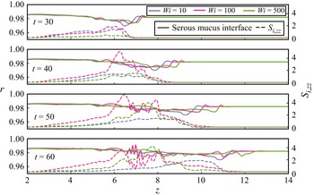
 Wi
Wi La=100
 Δp=2
Δp=2 μs−m=0.08
 Σs−m=0.1
 Bi=0
Bi=0 n=1
n=1 ϵs=0.015
 ϵ=0.05
 Wi
Wi Lp
Lp up
up ϵt=ϵ(zp−2)
 z=zp−2
 Δpw
Δpw Δτw
Δτw |∂zτw|max
 Wi∈[0,10,50,100,500,100]
 La=100
 Δp=2
Δp=2 μs−m=0.08
 Σs−m=0.1
 Wi=0
Wi=0 Bi=0
Bi=0 n=1
n=1 μg−m=1.5×10⁻³
 Bi
Bi n
n Lp
Lp Δpw
Δpw Δτw
Δτw |∂zτw|max
 up
up ϵt
ϵt La=100
 Δp=2
Δp=2 μs−m=0.08
 Σs−m=0.1
 ϵs=0.015
 ϵ=0.05
 μg−m=1.5×10⁻³
 Bi=0.1
 Bi=0.001
 n=0.3
n=0.3 Wi=100
 La=100
 μS=0.5
 Δp=2
Δp=2 μs−m=0.08
 Σs−m=0.1
 ϵs=0.015
 ϵ=0.05
 μ=1.5×10⁻³
 ρ=10−3
 λ=16
λ=16
 Bi
Bi n
n Wi=100
 Wi=1000
 Lp
Lp up
up ϵt
ϵt La=100
 Δp=2
Δp=2 μs−m=0.08
 ϵs=0.015
 ϵ=0.05
 Σs−m=0.1
 μg−m=1.5×10⁻³
 μs−m
μs−m ϵs
ϵs Δp
Δp La
La
 Δτw=max(τw)−min(τw)
 |∂zτw|max
 La=174
 ϵs=0.05
 μs−m=0.1
 Σs−m=0.1
 λ=6
λ=6
 Lp
Lp Δτw
Δτw Lp(t=0)=0.3
 La=100
 μs=0.1
 Σs−m=0.1
 Δp=2
Δp=2 Wi=100
 Bi=0
Bi=0 n=1
n=1 μg−m=1.5×10⁻³
 λ=8
λ=8
 Lp
Lp Δpw
Δpw Δτw
Δτw |∂zτw|max
 La=100
 μs=0.1
 Δp=2
Δp=2 Wi=0
Wi=0 Bi=0
Bi=0 n=1
n=1 ϵs=0.015
 ϵ=0.05
 ΔSw=maxSw(r=1)−minSw(r=1)
 Wi=100
 La=100
 μS=0.25
 Bi=0
Bi=0 n=1
n=1 Δp=1
Δp=1 μ=1.5×10⁻³
 ϵ=0.05
 Open access

