


1. Introduction
The intrusion of one fluid into another in a quasi-two-dimensional geometry is a flow that is known to be susceptible to instabilities, depending on the fluids involved. One well-known example is the viscous fingering observed in a Hele-Shaw cell when the intruding fluid is less viscous than the displaced fluid, which has been seen experimentally in the case of Newtonian fluids (Saffman & Taylor Reference Saffman and Taylor1958; Paterson Reference Paterson1981), as well as when at least one of the fluids is non-Newtonian (Lindner, Bonn & Meunier Reference Lindner, Bonn and Meunier2000; Dufresne, Ball & Balmforth Reference Dufresne, Ball and Balmforth2023; Hutchinson Reference Hutchinson2025). This Hele-Shaw cell geometry is characterised by horizontal rigid boundaries which cause the stresses in the fluids to be dominated by shear.
When the stress field is instead dominated by viscous extensional stresses, a different instability can be seen. This can occur in an axisymmetric environment when a shear-thinning fluid is extruded radially into a less viscous ambient fluid such that the intruding fluid has top and bottom interfaces that are effectively traction free, and therefore cannot support any leading-order shear. In a Hele-Shaw cell, this might occur if there are lubricating layers of the ambient fluid separating the intruding fluid from the rigid cell boundaries. The velocity of a ring of fluid decays radially as the fluid spreads outwards, as do the leading-order extensional strains that determine the fluid viscosity, leading to a viscosity field that increases radially. Under the influence of hoop stresses (i.e. viscous extensional stresses acting in the azimuthal direction to stretch the circular front as its circumference increases), it can be favourable for the region of high viscosity near the front, or nose, of the current to fracture rather than deform continuously. Indeed, fracturing has been observed experimentally at the front of such extrusions (Sayag & Worster Reference Sayag and Worster2019a ; Ball, Balmforth & Dufresne Reference Ball, Balmforth and Dufresne2021; Hutchinson & Worster Reference Hutchinson and Worster2025). Different dominant mechanisms for this process have been suggested, including a fluid instability (Sayag & Worster Reference Sayag and Worster2019b ), and a chemically governed instability, dependent on the fluids being used (Ball et al. Reference Ball, Balmforth and Dufresne2021). It is also known that the creep of ice sheets and shelves approximately obeys a power-law, shear-thinning rheology (Glen Reference Glen1955), and similar fractures have been observed in disintegrating floating ice shelves (Hughes Reference Hughes1983; Bassis et al. Reference Bassis, Fricker, Coleman and Minster2008).
This latter type of instability was investigated experimentally by Hutchinson & Worster (Reference Hutchinson and Worster2025), injecting a shear-thinning fluid (a solution of xanthan gum in water) into an ambient fluid of low viscosity and equal density (water) in a Hele-Shaw cell. Regions were observed where the xanthan gum displaced the water almost fully, effectively filling the gap between the upper and lower boundaries. Beyond these regions, the front of the xanthan gum layer was instead detached from the boundaries, being separated from them by substantial lubricating layers of water. Only in the latter regions, characterised by the dominance of extensional stresses due to the presence of the lubricating layers, were fracturing instabilities observed.
To investigate the role of the lubricating water layer, the experiments were modified by attaching discs to the upper and lower boundaries at the point of xanthan gum injection, so that, when the xanthan gum was extruded beyond these discs, there would be a lubricating layer of water of predetermined thickness between the gum and the boundaries. In this case, the fracturing instability created branch-like structures in the xanthan gum, separated by troughs that reached back to the edges of the discs. After some time, however, the less viscous bulk of the xanthan gum was seen to increase in thickness, building up behind the more viscous front and growing to fill the gap between the upper and lower boundaries, reproducing the geometry without the discs, at which point the fracturing instability lost its branch-like structure and was seen only in the regions that still possessed significant lubricating layers. We will show that a growth in the shear-thinning fluid layer thickness is also predicted in the absence of fracturing instabilities, and we will discuss the possibility of predicting the time at which the lubrication layers vanish in the experiments of Hutchinson & Worster (Reference Hutchinson and Worster2025).
In this paper, we construct a mathematical model to analyse the sorts of flow studied by Hutchinson & Worster (Reference Hutchinson and Worster2025) in the absence of any instabilities, keeping the assumption of axisymmetry throughout. Specifically, we study the axisymmetric extrusion of a shear-thinning fluid into an inviscid ambient fluid of the same density. A primary focus of our study is the thickening of the extruded layer caused by the radial increase in viscosity associated with a shear-thinning rheology. This basic phenomenon depends only on the viscosity decreasing with strain rate. So, although there are many different rheological models of shear-thinning fluids (see Ashkenazi & Boyko (Reference Ashkenazi and Boyko2025), who study various shear-thinning fluid models in axisymmetric, radial flow within an extruder, which is therefore shear dominated), we assume a simple power-law fluid, which allows significant analytical progress to be made. This brings our model in line with that of Ball & Balmforth (Reference Ball and Balmforth2021), who considered axisymmetric sliding flows of Herschel–Bulkley fluids (of which the power-law model is a special case), but with a key difference being our specific aim to probe the as yet unexplored limit of a neutrally buoyant flow. In § 2, we set out the governing equations and describe the boundary conditions appropriate to unconfined and confined extrusions at a constant volumetric rate, which are studied in more detail in §§ 3 and 4, respectively. For the unconfined case, we present numerical solutions to our mathematical model, and determine self-similar late-time behaviour for lower values of the power-law exponent $n\leqslant 3/2$
. We determine semi-analytical similarity solutions for those cases, and find that self-similar solutions do not exist for
$n\leqslant 3/2$
. We determine semi-analytical similarity solutions for those cases, and find that self-similar solutions do not exist for $n\gt 3/2$
. For the confined case, we derive late-time similarity solutions for all values of
$n\gt 3/2$
. For the confined case, we derive late-time similarity solutions for all values of $n$
, but focus on the shear-thinning results associated with
$n$
, but focus on the shear-thinning results associated with $n\gt 1$
. We compare those solutions with the analytical results of Sayag & Worster (Reference Sayag and Worster2019b
) for the axisymmetric extrusion of a power-law fluid at uniform thickness. In § 5, we compare the results of §§ 3 and 4 with the experimental results of Hutchinson & Worster (Reference Hutchinson and Worster2025), and discuss potential developments of the theory needed to improve predictions.
$n\gt 1$
. We compare those solutions with the analytical results of Sayag & Worster (Reference Sayag and Worster2019b
) for the axisymmetric extrusion of a power-law fluid at uniform thickness. In § 5, we compare the results of §§ 3 and 4 with the experimental results of Hutchinson & Worster (Reference Hutchinson and Worster2025), and discuss potential developments of the theory needed to improve predictions.
Schematic diagrams of shear-thinning fluid being extruded axisymmetrically from the gap between parallel, circular discs of radius $r_0$
separated by a distance
$r_0$
separated by a distance $2h_0$
. (
$2h_0$
. ( $a$
) Unconfined extrusion into an inviscid environment; the fluid is free to expand vertically. (
$a$
) Unconfined extrusion into an inviscid environment; the fluid is free to expand vertically. ( $b$
) Confined extrusion between parallel plates into an inviscid ambient; the fluid fills the gap between the plates up to a radius
$b$
) Confined extrusion between parallel plates into an inviscid ambient; the fluid fills the gap between the plates up to a radius $r_G(t)$
. In both cases, the end of the current is at radius
$r_G(t)$
. In both cases, the end of the current is at radius $r_{\!N}(t)$
.
$r_{\!N}(t)$
.

2. Unconfined and confined axisymmetric extrusions
We consider axisymmetric extrusion of a viscous fluid at a constant volume flux $Q$
from a cylindrical source of radius
$Q$
from a cylindrical source of radius $r_0$
and height
$r_0$
and height $2 h_0$
in either an unconfined (figure 1
$2 h_0$
in either an unconfined (figure 1 $a$
) or vertically confined (figure 1
$a$
) or vertically confined (figure 1 $b$
) geometry initially occupied by an inviscid Newtonian ambient fluid. We assume the injected and ambient fluid are of similar densities, and hence ignore the effects of gravity. Nevertheless, we describe the
$b$
) geometry initially occupied by an inviscid Newtonian ambient fluid. We assume the injected and ambient fluid are of similar densities, and hence ignore the effects of gravity. Nevertheless, we describe the $z$
-direction as vertical and the orthogonal plane as horizontal, and use cylindrical polar coordinates
$z$
-direction as vertical and the orthogonal plane as horizontal, and use cylindrical polar coordinates $(r, \theta , z)$
, in which
$(r, \theta , z)$
, in which $r$
measures the radial distance from the
$r$
measures the radial distance from the $z$
-axis, the axis of symmetry. We also assume that the effects of inertia are negligible.
$z$
-axis, the axis of symmetry. We also assume that the effects of inertia are negligible.
In the unconfined case, outside the cylindrical source and for times $t\gt 0$
, the intruding fluid occupies the region
$t\gt 0$
, the intruding fluid occupies the region $|z| \lt h(r, t)$
,
$|z| \lt h(r, t)$
, $r_0 \lt r \lt r_{\!N}(t)$
, where
$r_0 \lt r \lt r_{\!N}(t)$
, where $2 h(r,t)$
is the thickness of the current and
$2 h(r,t)$
is the thickness of the current and $r_{\!N}(t)$
is its leading edge. In the confined case, the intruding fluid occupies two regions: one in which the fluid fills the entire gap between the two plates,
$r_{\!N}(t)$
is its leading edge. In the confined case, the intruding fluid occupies two regions: one in which the fluid fills the entire gap between the two plates, $|z| \lt h_0$
,
$|z| \lt h_0$
, $r_0 \lt r \lt r_G(t)$
, and another in which the fluid partially fills the gap,
$r_0 \lt r \lt r_G(t)$
, and another in which the fluid partially fills the gap, $|z| \lt h(r, t)$
,
$|z| \lt h(r, t)$
, $r_G(t) \lt r \lt r_{\!N}(t)$
, where
$r_G(t) \lt r \lt r_{\!N}(t)$
, where $r_G(t)$
is the grounding line. We use the thin-film approximation that radial length scales are much larger than axial length scales, specifically that
$r_G(t)$
is the grounding line. We use the thin-film approximation that radial length scales are much larger than axial length scales, specifically that $h \ll r_{\!N} - r_0$
and
$h \ll r_{\!N} - r_0$
and $h \ll r_{\!N} - r_G$
for the unconfined and confined geometries, respectively.
$h \ll r_{\!N} - r_G$
for the unconfined and confined geometries, respectively.
Since the ambient fluid is inviscid, it exerts zero shear stress on the intruding fluid, and so the near-horizontal stress-free interfaces at $z=\pm h(r,t)$
cannot support any vertical shear in the intruding fluid to leading order in the aspect ratio. As a result, the leading-order flow in the intruding fluid is quasi-parallel and vertically uniform where it is in contact with the ambient fluid, with horizontal velocity of the form
$z=\pm h(r,t)$
cannot support any vertical shear in the intruding fluid to leading order in the aspect ratio. As a result, the leading-order flow in the intruding fluid is quasi-parallel and vertically uniform where it is in contact with the ambient fluid, with horizontal velocity of the form ${\boldsymbol u} = u(r,t) \boldsymbol{\hat {r}}$
, independent of
${\boldsymbol u} = u(r,t) \boldsymbol{\hat {r}}$
, independent of $\theta$
and the vertical coordinate
$\theta$
and the vertical coordinate $z$
. Any shear generated in the confined region would be dissipated within a distance
$z$
. Any shear generated in the confined region would be dissipated within a distance $h_0$
of the grounding line, which is negligible given the thin-film approximation. Therefore, for ease of discussion, we also assume that the confining walls are stress free, so only consider extensional stresses throughout.
$h_0$
of the grounding line, which is negligible given the thin-film approximation. Therefore, for ease of discussion, we also assume that the confining walls are stress free, so only consider extensional stresses throughout.
The general equations governing such quasi-two-dimensional extensional flows (Pegler, Lister & Worster Reference Pegler, Lister and Worster2012; Pegler & Worster Reference Pegler and Worster2012) in the absence of gravity are
 \begin{equation} \boldsymbol{\nabla }(\mu h \boldsymbol {\nabla }\boldsymbol{\cdot }{\boldsymbol u}) + \boldsymbol{\nabla }\boldsymbol{\cdot }(\mu h \unicode{x1D65A}) = {\boldsymbol 0}, \end{equation}
representing the radial force balance, and
 \begin{equation} \frac {\partial h}{\partial t} + \boldsymbol{\nabla }\boldsymbol{\cdot }(h{\boldsymbol u}) = 0, \end{equation}
representing conservation of mass, where $\boldsymbol{\nabla}$
is the horizontal part of the gradient operator and
$\boldsymbol{\nabla}$
is the horizontal part of the gradient operator and $\unicode{x1D65A} \equiv [\boldsymbol{\nabla }{\boldsymbol u} + ( \boldsymbol{\nabla }{\boldsymbol u} ) ^{{T}}]/2$
is the horizontal rate-of-strain tensor. We consider power-law rheologies in which the dynamic viscosity is given by
$\unicode{x1D65A} \equiv [\boldsymbol{\nabla }{\boldsymbol u} + ( \boldsymbol{\nabla }{\boldsymbol u} ) ^{{T}}]/2$
is the horizontal rate-of-strain tensor. We consider power-law rheologies in which the dynamic viscosity is given by
 \begin{equation} \mu = \tilde \mu\! \left [{\frac {1}{2}}\unicode{x1D640}{:}\unicode{x1D640}\right ]^{(1-n)/(2n)} \equiv \tilde \mu\! \left [\frac {1}{2}\big ( \unicode{x1D65A}{:}\unicode{x1D65A} + ( \boldsymbol{\nabla }\boldsymbol{\cdot }{\boldsymbol u})^2\big )\right ]^{(1-n)/(2n)} , \end{equation}
where $\unicode{x1D640}$
is the full three-dimensional rate-of-strain tensor and
$\unicode{x1D640}$
is the full three-dimensional rate-of-strain tensor and $\tilde \mu$
and
$\tilde \mu$
and $n$
are constants. Newtonian fluids have
$n$
are constants. Newtonian fluids have $n=1$
, while shear-thinning fluids have
$n=1$
, while shear-thinning fluids have $n \gt 1$
.
$n \gt 1$
.
For horizontal velocities of the form ${\boldsymbol u} = (u(r, t), 0)$
, the viscosity (2.3) is
${\boldsymbol u} = (u(r, t), 0)$
, the viscosity (2.3) is
 \begin{equation} \mu =\tilde {\mu }\! \left [u_r^2+\frac {u u_r}{r} +\frac {u^2}{r^2} \right ]^{(1-n)/(2n)}, \end{equation}
which is a decreasing function of the strain rate $(({1}/{2})\unicode{x1D640}{:}\unicode{x1D640})^{1/2}$
for
$(({1}/{2})\unicode{x1D640}{:}\unicode{x1D640})^{1/2}$
for $n\gt 1$
. The force balance (2.1) and mass conservation (2.2) become
$n\gt 1$
. The force balance (2.1) and mass conservation (2.2) become
 \begin{equation} 2 \mu h\! \left (u_{rr}+\frac {u_r}{r} - \frac {u}{r^2} \right ) +(\mu h)_r\! \left (2 u_r+\frac {u}{r} \right )=0, \end{equation}
 \begin{equation} h_t + {1\over r}(r u h)_r = 0, \end{equation}
and are subject to the kinematic boundary conditions
 \begin{equation} h = h_0, \quad u =U_0\equiv {Q\over 4\pi h_0 r_0 } \quad \hbox{at} \quad r = r_0, \end{equation}
for the unconfined case, and
 \begin{equation} h = h_0, \quad u =U_G\equiv {Q\over 4\pi h_0 r_G} \quad \hbox{at} \quad r = r_G, \end{equation}
for the confined case. The position of the front, or nose, of the current $r_{\!N}(t)$
is determined kinematically from
$r_{\!N}(t)$
is determined kinematically from
 \begin{equation} \dot r_{\!N} = u(r_{\!N}, t). \end{equation}
The remaining dynamic boundary condition
 \begin{equation} (\boldsymbol{\nabla }\boldsymbol{\cdot }{\boldsymbol u}){\boldsymbol n} + \unicode{x1D65A} \boldsymbol{\cdot }{\boldsymbol n} = \textbf {0} \quad \hbox{at} \quad r = r_{\!N}(t), \end{equation}
where $\boldsymbol n=\boldsymbol{\hat {r}}$
is the unit horizontal normal to the edge, represents zero horizontal force applied to the end of the current. In the case under study, this condition takes the form
$\boldsymbol n=\boldsymbol{\hat {r}}$
is the unit horizontal normal to the edge, represents zero horizontal force applied to the end of the current. In the case under study, this condition takes the form
 \begin{equation} 2u_r + {u\over r} = 0 \quad \hbox{at} \quad r = r_{\!N}(t). \end{equation}
We assume that the region $r\gt r_0$
outside the cylindrical source is initially completely occupied by an inviscid fluid, and hence we impose the initial condition
$r\gt r_0$
outside the cylindrical source is initially completely occupied by an inviscid fluid, and hence we impose the initial condition
 \begin{equation} r_{\!N}=r_0 \quad \hbox{at} \quad t=0. \end{equation}
3. Unconfined extrusion
In this section, we consider the axisymmetric injection of Newtonian and power-law fluids displacing an inviscid fluid in the unconfined geometry shown in figure 1( $a$
). Equations (2.5a
) and (2.5b
), with viscosity given by (2.4), subject to the boundary conditions (2.6), (2.8) and (2.10), as well as the initial condition (2.11), are first solved numerically (§§ 3.1 and 3.3 respectively for the two rheologies). When appropriate, similarity solutions are determined semi-analytically to describe the late-time behaviour (§§ 3.2 and 3.4, respectively).
$a$
). Equations (2.5a
) and (2.5b
), with viscosity given by (2.4), subject to the boundary conditions (2.6), (2.8) and (2.10), as well as the initial condition (2.11), are first solved numerically (§§ 3.1 and 3.3 respectively for the two rheologies). When appropriate, similarity solutions are determined semi-analytically to describe the late-time behaviour (§§ 3.2 and 3.4, respectively).
3.1. Unconfined extrusion of a Newtonian fluid
If the injected fluid is Newtonian then the viscosity $\mu$
is constant and can be factored out of (2.5a
). We introduce the scalings
$\mu$
is constant and can be factored out of (2.5a
). We introduce the scalings
 \begin{equation} h \sim h_0, \ \ \ r \sim r_0, \ \ \ u \sim U_0 \equiv \frac {Q}{4 \pi r_0 h_0}, \ \ \ t \sim \frac {r_0}{U_0}. \end{equation}
The governing equations and boundary conditions are unchanged by these scalings, barring (2.6) and (2.11), which, in dimensionless form, become
 \begin{equation} h = 1, \quad u = 1 \quad \hbox{at} \quad r = 1, \end{equation}
 \begin{equation} r_{\!N}=1 \quad \hbox{at} \quad t=0. \end{equation}
As an aside, note that in two dimensions, with the velocity $u$
in the
$u$
in the $x$
direction, there are no hoop stresses and the solution of the equivalent dimensionless equations is simply
$x$
direction, there are no hoop stresses and the solution of the equivalent dimensionless equations is simply $u\equiv 1$
,
$u\equiv 1$
, $h\equiv 1$
, with the nose position at
$h\equiv 1$
, with the nose position at $x_N(t) = 1+t$
(assuming extrusion from
$x_N(t) = 1+t$
(assuming extrusion from $x_0=1$
).
$x_0=1$
).
We start here by determining full numerical solutions to the extrusion problem. We map the domain $[1, r_{\!N}]$
onto
$[1, r_{\!N}]$
onto $[0, 1]$
using the independent variable
$[0, 1]$
using the independent variable
 \begin{equation} X(r,t) = {r - 1\over L(t)}, \quad \hbox{where} \quad L(t) = r_{\!N}(t) - 1. \end{equation}
We also introduce the dependent variable
 \begin{equation} y(r, t) = \textit{ru}(r, t), \end{equation}
which remains bounded as $r\to 0$
. Expressing the dependent variables as
$r\to 0$
. Expressing the dependent variables as $y=y(X,t)$
and
$y=y(X,t)$
and $h=h(X,t)$
, the governing equations then become
$h=h(X,t)$
, the governing equations then become
 \begin{equation} 2h\!\left ({y_{XX}\over L} - {y_X\over 1+\textit{LX}}\right ) + h_X\!\left ( {2y_X\over L} - {y\over 1+\textit{LX}}\right ) = 0, \end{equation}
 \begin{equation} h_t - {\dot L\over L} X h_X + {(hy)_X\over L(1+\textit{LX})} = 0, \end{equation}
subject to boundary and initial conditions
 \begin{equation} h = 1, \quad y = 1 \quad \hbox{at} \quad X = 0, \end{equation}
 \begin{equation} {2y_X\over L} - {y\over 1+L} = 0, \quad \dot L = {y\over 1+L} \quad \hbox{at} \quad X = 1, \end{equation}
 \begin{equation} L = 0 \quad \hbox{at} \quad t = 0. \end{equation}
These equations are singular in the limit $L\to 0$
, when the initial distribution
$L\to 0$
, when the initial distribution $h(X,0)$
is condensed into the point
$h(X,0)$
is condensed into the point $r=1$
. For consistency with the boundary condition (3.6a
), we define the initial distribution
$r=1$
. For consistency with the boundary condition (3.6a
), we define the initial distribution
 \begin{equation} h(X,0)=1, \end{equation}
to avoid the function $h(r,t)$
being multivalued at
$h(r,t)$
being multivalued at $t=0$
.
$t=0$
.
To avoid this singularity when integrating the equations numerically, we find the early-time asymptotic solution. Letting
 \begin{equation} y = 1 + L(t) Y(X,t) + O(L^2), \quad h = 1+ L(t) H(X,t)+ O(L^2), \end{equation}
we find that, after expanding in powers of $L$
, the momentum equation, (3.5a
), has leading order
$L$
, the momentum equation, (3.5a
), has leading order $Y_{XX}=0$
, the evolution equation, (3.5b
), has leading order
$Y_{XX}=0$
, the evolution equation, (3.5b
), has leading order $\dot LH-\dot LXH_X+Y_X+H_X=0$
and the boundary conditions (3.6a
–
d
) have leading order
$\dot LH-\dot LXH_X+Y_X+H_X=0$
and the boundary conditions (3.6a
–
d
) have leading order $H=Y=0$
at
$H=Y=0$
at $X=0$
,
$X=0$
, $Y_X= {1}/{2}$
at
$Y_X= {1}/{2}$
at $X=1$
and
$X=1$
and $\dot L=1$
, respectively. Solving these equations, along with
$\dot L=1$
, respectively. Solving these equations, along with $L=0$
at
$L=0$
at $t=0$
, gives
$t=0$
, gives
 \begin{equation} y \sim 1 + \frac {\textit{LX}}{2}, \quad h \sim 1 - \frac {\textit{LX}}{2}, \quad L \sim t. \end{equation}
The small-time evolution of $L(t)$
is illustrated in the figure 2(
$L(t)$
is illustrated in the figure 2( $b$
) inset. Ball & Balmforth (Reference Ball and Balmforth2021) derive an equivalent small-time solution for a floating Newtonian extrusion, with an additional term in each of
$b$
) inset. Ball & Balmforth (Reference Ball and Balmforth2021) derive an equivalent small-time solution for a floating Newtonian extrusion, with an additional term in each of $Y$
and
$Y$
and $H$
corresponding to a hydrostatic pressure term in the force balance at the nose (3.6c
). The effect of buoyancy on the solution is discussed further in § 3.2.1.
$H$
corresponding to a hydrostatic pressure term in the force balance at the nose (3.6c
). The effect of buoyancy on the solution is discussed further in § 3.2.1.
The solution to (3.5)–(3.6) for the extrusion of a Newtonian fluid. ( $a$
) Plots of the current half-thickness
$a$
) Plots of the current half-thickness $h$
at dimensionless times
$h$
at dimensionless times $t=$
5, 20, 100, 500 and 2000, from left to right. The dashed curve is
$t=$
5, 20, 100, 500 and 2000, from left to right. The dashed curve is $h_N={r_{\!N}}^{-1/2}$
, as predicted by (3.11b
) for the thickness of the intruding fluid at the nose. (
$h_N={r_{\!N}}^{-1/2}$
, as predicted by (3.11b
) for the thickness of the intruding fluid at the nose. ( $b$
) The same results shown in (
$b$
) The same results shown in ( $a$
) plotted in similarity space, according to the scalings defined in (3.12). The similarity solution to (3.13) with
$a$
) plotted in similarity space, according to the scalings defined in (3.12). The similarity solution to (3.13) with $\eta _N\approx 1.71$
is shown in dashed red. The black dots indicate the asymptotic results (3.18) and (3.20). The inset shows a log–log plot of the evolution of the current length
$\eta _N\approx 1.71$
is shown in dashed red. The black dots indicate the asymptotic results (3.18) and (3.20). The inset shows a log–log plot of the evolution of the current length $L(t)\equiv r_{\!N}(t)-1$
, illustrating the transition from the small-time solution (3.9) to the similarity solution
$L(t)\equiv r_{\!N}(t)-1$
, illustrating the transition from the small-time solution (3.9) to the similarity solution $L=\eta _Nt^{1/2}-1\sim \eta _Nt^{1/2}$
, with the asymptotic expressions plotted in dashed red. (
$L=\eta _Nt^{1/2}-1\sim \eta _Nt^{1/2}$
, with the asymptotic expressions plotted in dashed red. ( $c$
) Plots of the similarity solution profiles for
$c$
) Plots of the similarity solution profiles for $y\equiv ru$
and
$y\equiv ru$
and $u$
.
$u$
.

Figure 2( $a$
,
$a$
, $b$
) shows the numerical solution of (3.5)–(3.6) starting from this asymptotic solution. The transformation (3.3) means that numerical solution of the equations was performed on a fixed grid. We used central differences for spatial derivatives and a second-order, implicit midpoint scheme in time.
$b$
) shows the numerical solution of (3.5)–(3.6) starting from this asymptotic solution. The transformation (3.3) means that numerical solution of the equations was performed on a fixed grid. We used central differences for spatial derivatives and a second-order, implicit midpoint scheme in time.
We see that $h(r_{\!N}, t) \ne 0$
but approaches zero on a similar time scale to that taken for the extent of the intruding flow to exceed the radius of injection significantly. To understand the evolution of
$h(r_{\!N}, t) \ne 0$
but approaches zero on a similar time scale to that taken for the extent of the intruding flow to exceed the radius of injection significantly. To understand the evolution of $h_N = h(r_{\!N}(t), t)$
, we evaluate (2.5b
) at
$h_N = h(r_{\!N}(t), t)$
, we evaluate (2.5b
) at $r=r_{\!N}(t)$
and use the result to write
$r=r_{\!N}(t)$
and use the result to write
 \begin{equation} \dot h_N \equiv \frac {D h}{D t}(r_{\!N},t) = -h_N\! \left (\frac {u(r_{\!N},t)}{r_{\!N}} + \frac {\partial u}{\partial r}(r_{\!N},t) \right )\!. \end{equation}
 \begin{equation} 2 \dot h_N +h_N \frac {\dot r_{\!N}}{r_{\!N}} =0, \quad \hbox{whence} \quad h_N = r_{\!N}^{-1/2}, \end{equation}
having used the boundary condition (3.2a
) and the initial condition (3.2c
) to determine that $h_N=1$
when
$h_N=1$
when $r_{\!N}=1$
. Note that (2.8) and (2.10), and hence also this result, are independent of the rheology of the fluid, and can be seen for different power-law exponents in figures 3 and 4. The relation (3.11b
) is plotted for a Newtonian fluid as the dashed curve in figure 2(
$r_{\!N}=1$
. Note that (2.8) and (2.10), and hence also this result, are independent of the rheology of the fluid, and can be seen for different power-law exponents in figures 3 and 4. The relation (3.11b
) is plotted for a Newtonian fluid as the dashed curve in figure 2( $a$
).
$a$
).
Now, $L(t)=r_{\!N}(t)-1$
, and on short time scales, we found that
$L(t)=r_{\!N}(t)-1$
, and on short time scales, we found that $L \sim t$
(see (3.9c
)), giving
$L \sim t$
(see (3.9c
)), giving $r_{\!N} \sim 1+t$
and therefore
$r_{\!N} \sim 1+t$
and therefore $h_N \sim (1+t)^{-1/2} \sim 1-t/2$
, which is consistent with our approximation for
$h_N \sim (1+t)^{-1/2} \sim 1-t/2$
, which is consistent with our approximation for $h$
in (3.9b
) when evaluated at the endpoint
$h$
in (3.9b
) when evaluated at the endpoint $X=1$
. We will soon show that at late times,
$X=1$
. We will soon show that at late times, $r_{\!N} \sim t^{1/2}$
so that
$r_{\!N} \sim t^{1/2}$
so that $h_N \sim t^{-1/4}$
, which represents a slow, algebraic decay towards
$h_N \sim t^{-1/4}$
, which represents a slow, algebraic decay towards $h_N=0$
.
$h_N=0$
.
3.2. Similarity solution for extrusion of a Newtonian fluid
On long time scales, formally as $r_{\!N}\to \infty$
, the fluid can be considered to be extruded from a line source occupying
$r_{\!N}\to \infty$
, the fluid can be considered to be extruded from a line source occupying $r=0$
,
$r=0$
, $-1\leqslant z\leqslant 1$
. This case was considered by Pegler & Worster (Reference Pegler and Worster2012), where they found that the equations admitted a similarity solution at early times in their scenario, when the effects of buoyancy were negligible. They then used this similarity solution as an initial condition for numerical calculations of buoyancy-driven extension. The physical relevance of this similarity solution to their flow is discussed in § 3.2.1. We can recover their similarity solution by considering a radial similarity variable that is independent of
$-1\leqslant z\leqslant 1$
. This case was considered by Pegler & Worster (Reference Pegler and Worster2012), where they found that the equations admitted a similarity solution at early times in their scenario, when the effects of buoyancy were negligible. They then used this similarity solution as an initial condition for numerical calculations of buoyancy-driven extension. The physical relevance of this similarity solution to their flow is discussed in § 3.2.1. We can recover their similarity solution by considering a radial similarity variable that is independent of $r_0$
. From (3.1),
$r_0$
. From (3.1), $t^{-1/2} r$
is the only combination of the dimensionless variables
$t^{-1/2} r$
is the only combination of the dimensionless variables $t$
and
$t$
and $r$
that is independent of
$r$
that is independent of $r_0$
, and so we let
$r_0$
, and so we let
 \begin{equation} h(r, t) = h(\eta ), \quad y(r, t) = y(\eta ), \quad \hbox{where} \quad \eta = {r\over t^{1/2}}. \end{equation}
By plotting $h$
against
$h$
against $r/t^{1/2}$
for the transient problem (3.5)–(3.6), we can verify this scaling and approximate the similarity solution by observing convergence at late time, as shown in figure 2(
$r/t^{1/2}$
for the transient problem (3.5)–(3.6), we can verify this scaling and approximate the similarity solution by observing convergence at late time, as shown in figure 2( $b$
).
$b$
).
For completeness and ease of reference, we present the similarity equations for $y(\eta )$
and
$y(\eta )$
and $h(\eta )$
here as
$h(\eta )$
here as
 \begin{equation} 2 h\! \left (y'' - {y'\over \eta }\right ) + h'\! \left (2 y' - {y\over \eta }\right ) = 0, \end{equation}
 \begin{equation} \left (y - {\eta ^2\over 2}\right ) h' + h y' = 0, \end{equation}
 \begin{equation} y = 1, \quad h = 1 \quad \hbox{at} \quad \eta = 0, \end{equation}
 \begin{equation} y = {\eta _N^2\over 2}, \quad y' = {\eta _N\over 4} \quad \hbox{at} \quad \eta = \eta _N, \end{equation}
where $\eta _N = t^{-1/2}r_{\!N}$
, and primes denote
$\eta _N = t^{-1/2}r_{\!N}$
, and primes denote $\text{d}/\text{d}\eta$
.
$\text{d}/\text{d}\eta$
.
We eliminate $h$
between (3.13a
) and (3.13b
) to give
$h$
between (3.13a
) and (3.13b
) to give
 \begin{equation} 2\!\left (y - {\eta ^2\over 2}\right ) \left (y'' - {y'\over \eta }\right ) - \left (2 y' - {y\over \eta }\right )y' = 0, \end{equation}
which we solved in Matlab using the in-built integrator ode45, shooting backwards from the nose to find the value $\eta _N\approx 1.71$
that gives
$\eta _N\approx 1.71$
that gives $y = 1$
at
$y = 1$
at $\eta =0$
, in agreement with the value found by Pegler & Worster (Reference Pegler and Worster2012). Given the boundary condition (3.13e
), it is clear that this differential equation is singular at
$\eta =0$
, in agreement with the value found by Pegler & Worster (Reference Pegler and Worster2012). Given the boundary condition (3.13e
), it is clear that this differential equation is singular at $\eta = \eta _N$
. However, it has a removable singularity, and we use a second-order Taylor expansion to show that
$\eta = \eta _N$
. However, it has a removable singularity, and we use a second-order Taylor expansion to show that $y''(\eta _N) = 5/32$
. This expression allows us to avoid the singularity at
$y''(\eta _N) = 5/32$
. This expression allows us to avoid the singularity at $\eta _N$
, by writing (3.14) as
$\eta _N$
, by writing (3.14) as
 \begin{equation} y''=\left \{\begin{matrix}\left (\frac {2\eta y'+y-\eta ^2}{2\eta (y-\eta ^2/2)}\right )y'&\text{for }\eta \lt \eta _N\\[10pt]5/32&\text{for }\eta =\eta _N,\end{matrix}\right . \end{equation}
and integrating this new equation backwards from $\eta _N$
, applying (3.13e
,
f
) as the initial condition, and ending at
$\eta _N$
, applying (3.13e
,
f
) as the initial condition, and ending at $\epsilon _0=10^{-8}$
.
$\epsilon _0=10^{-8}$
.
Once $y(\eta )$
has been determined, it is in principle straightforward to integrate (3.13b
) using quadrature to evaluate
$y(\eta )$
has been determined, it is in principle straightforward to integrate (3.13b
) using quadrature to evaluate
 \begin{align} h = \exp \int _0^\eta {2y'(\xi )\over \xi ^2 - 2y(\xi )}\, \text d\xi . \end{align}
However, it proved expedient to integrate (3.13b
) for $h$
numerically alongside the integration for
$h$
numerically alongside the integration for $y$
, starting from the asymptotic solution near the nose,
$y$
, starting from the asymptotic solution near the nose, $h \sim A(\eta _N - \eta )^{1/3}$
(see (3.41) for a derivation of the most general form of this asymptote). We write
$h \sim A(\eta _N - \eta )^{1/3}$
(see (3.41) for a derivation of the most general form of this asymptote). We write $\phi \equiv (\eta _N-\eta )^{-1/3}h$
, and substitute this expression into (3.13b
) to find
$\phi \equiv (\eta _N-\eta )^{-1/3}h$
, and substitute this expression into (3.13b
) to find
 \begin{align} \phi '=\left (\frac {-3(\eta _N-\eta )y'+y-\eta ^2/2}{3(\eta _N-\eta )(y-\eta ^2/2)}\right )\phi . \end{align}
Expanding the term in brackets with a second-order Taylor expansion in $(\eta _N-\eta )$
, and substituting in (3.13e
,
f
) and the value
$(\eta _N-\eta )$
, and substituting in (3.13e
,
f
) and the value $y''(\eta _N)=5/32$
found above, we find that
$y''(\eta _N)=5/32$
found above, we find that $\phi '(\eta _N)=A/(48\eta _N)$
, where
$\phi '(\eta _N)=A/(48\eta _N)$
, where $A=\phi (\eta _N)$
. This allows us to integrate (3.13b
) directly from
$A=\phi (\eta _N)$
. This allows us to integrate (3.13b
) directly from $\eta _N$
, using the technique described in (3.15). We shoot to determine
$\eta _N$
, using the technique described in (3.15). We shoot to determine $A\approx 0.904$
, and thus
$A\approx 0.904$
, and thus
 \begin{align} h \sim 0.904(\eta _N - \eta )^{1/3} \quad \hbox{as} \quad \eta \to \eta _N, \end{align}
in agreement with Pegler & Worster (Reference Pegler and Worster2012).
An asymptotic approximation to $h$
near
$h$
near $\eta = 0$
can be determined straightforwardly as follows. Firstly, (3.13b
) shows that
$\eta = 0$
can be determined straightforwardly as follows. Firstly, (3.13b
) shows that $(hy)' = 0$
to leading order in
$(hy)' = 0$
to leading order in $\eta$
, and from (3.13c
,
d
),
$\eta$
, and from (3.13c
,
d
), $h y =1$
. Therefore, writing
$h y =1$
. Therefore, writing $y = 1+\delta (\eta )$
, with
$y = 1+\delta (\eta )$
, with $\delta \to 0$
as
$\delta \to 0$
as $\eta \to 0$
, we can deduce that
$\eta \to 0$
, we can deduce that $h\sim 1 - \delta (\eta )$
as
$h\sim 1 - \delta (\eta )$
as $\eta \to 0$
. With these asymptotic expressions, it is straightforward to show that the dominant balance in (3.13a
) is
$\eta \to 0$
. With these asymptotic expressions, it is straightforward to show that the dominant balance in (3.13a
) is
 \begin{equation} 2 \delta '' - {\delta '\over \eta } = 0, \end{equation}
whence $\delta \sim B\eta ^{3/2}$
, for some constant
$\delta \sim B\eta ^{3/2}$
, for some constant $B$
. We determined
$B$
. We determined $B = 0.190$
by evaluating
$B = 0.190$
by evaluating $B \sim -(2/3)h'(\eta )/\eta ^{1/2}$
at
$B \sim -(2/3)h'(\eta )/\eta ^{1/2}$
at $\eta = \epsilon _0$
where the value of
$\eta = \epsilon _0$
where the value of $h'(\epsilon _0)$
is obtained from the full numerical solution to (3.13b
). Given now that
$h'(\epsilon _0)$
is obtained from the full numerical solution to (3.13b
). Given now that
 \begin{equation} h \sim 1 - 0.190\eta ^{3/2} \quad \hbox{as} \quad \eta \to 0, \end{equation}
the intruding fluid remains very close to $h=1$
near the point of extrusion. The similarity solution for
$h=1$
near the point of extrusion. The similarity solution for $h$
and these asymptotic approximations are shown in figure 2(
$h$
and these asymptotic approximations are shown in figure 2( $b$
), and the corresponding solutions for
$b$
), and the corresponding solutions for $y$
and the similarity velocity
$y$
and the similarity velocity $y/\eta \equiv u/t^{-1/2}$
are plotted in figure 2(
$y/\eta \equiv u/t^{-1/2}$
are plotted in figure 2( $c$
).
$c$
).
Given that $h\lt 1$
throughout the domain
$h\lt 1$
throughout the domain $r\gt 1$
, the solutions in this section also describe the extrusion of fluid into a confining channel containing an inviscid ambient fluid, a geometry that is discussed further in § 4. However, the fact that
$r\gt 1$
, the solutions in this section also describe the extrusion of fluid into a confining channel containing an inviscid ambient fluid, a geometry that is discussed further in § 4. However, the fact that $h$
is very close to unity near the radius of extrusion means that if the ambient fluid has any viscosity, no matter how small, then the assumption that the intruding fluid feels no tangential stress is invalid in the neighbourhood of the source. This is worth exploring but is beyond the scope of the current paper.
$h$
is very close to unity near the radius of extrusion means that if the ambient fluid has any viscosity, no matter how small, then the assumption that the intruding fluid feels no tangential stress is invalid in the neighbourhood of the source. This is worth exploring but is beyond the scope of the current paper.
3.2.1. Evolution of a buoyant current
Pegler & Worster (Reference Pegler and Worster2012) consider a buoyant current with density $\rho$
floating on an inviscid fluid with density
$\rho$
floating on an inviscid fluid with density $\rho _w$
, produced by a line source with height
$\rho _w$
, produced by a line source with height $2h_0$
. They find an early-time similarity solution, before buoyancy effects become significant, which is replaced by a late-time, buoyancy-dominated solution with a steady
$2h_0$
. They find an early-time similarity solution, before buoyancy effects become significant, which is replaced by a late-time, buoyancy-dominated solution with a steady $h$
profile, and a nose that advances with
$h$
profile, and a nose that advances with $r_{\!N}\sim t$
.
$r_{\!N}\sim t$
.
Their formulation is equivalent to the set-up in figure 1( $a$
), with the addition of a buoyancy force, and with
$a$
), with the addition of a buoyancy force, and with $r_0$
set to 0. This reproduces the condition for the scalings in (3.12) to be valid, namely independence from the initial extrusion radius, and hence the late-time similarity solution found above for an extruded Newtonian current is identically their early-time solution, before the effects of buoyancy become significant.
$r_0$
set to 0. This reproduces the condition for the scalings in (3.12) to be valid, namely independence from the initial extrusion radius, and hence the late-time similarity solution found above for an extruded Newtonian current is identically their early-time solution, before the effects of buoyancy become significant.
They identify a buoyancy time scale and radial length scale
 \begin{equation} \mathcal{T}\equiv \frac {\mu }{2\rho g'h_0},\quad \mathcal{R}\equiv \left (\frac {\mu Q}{8\pi \rho g'h_0^2}\right )^{1/2}, \end{equation}
respectively, where $g'\equiv (\rho _w-\rho )g/\rho _w$
is the reduced gravity, and all other parameters are as defined in § 2. They find convergence from the purely extensional similarity solution to the buoyancy-driven similarity solution for dimensionless time
$g'\equiv (\rho _w-\rho )g/\rho _w$
is the reduced gravity, and all other parameters are as defined in § 2. They find convergence from the purely extensional similarity solution to the buoyancy-driven similarity solution for dimensionless time $t\gtrsim 100$
, non-dimensionalised using (3.21).
$t\gtrsim 100$
, non-dimensionalised using (3.21).
However, if we consider a modification of their set-up, with extrusion at a finite radius $r_0$
rather than a line source, we can estimate the evolution of the flow by comparing the onset of buoyancy effects found in their paper with the onset of extensional effects described in § 3.1. Here, in the case of a neutrally buoyant fluid extruded from a finite radius, we find convergence to the purely extensional similarity solution around dimensionless time
$r_0$
rather than a line source, we can estimate the evolution of the flow by comparing the onset of buoyancy effects found in their paper with the onset of extensional effects described in § 3.1. Here, in the case of a neutrally buoyant fluid extruded from a finite radius, we find convergence to the purely extensional similarity solution around dimensionless time $t\gtrsim 100$
(see figure 2
$t\gtrsim 100$
(see figure 2 $b$
), but non-dimensionalised now using (3.1). Therefore, in the case of extrusion of a buoyant fluid from a cylindrical source, the purely extensional similarity solution is only expected to develop if the buoyancy time scale given in (3.21) is much larger than the geometric time scale given in (3.1), or, equivalently, the buoyancy radius is much larger than the extrusion radius, expressible as
$b$
), but non-dimensionalised now using (3.1). Therefore, in the case of extrusion of a buoyant fluid from a cylindrical source, the purely extensional similarity solution is only expected to develop if the buoyancy time scale given in (3.21) is much larger than the geometric time scale given in (3.1), or, equivalently, the buoyancy radius is much larger than the extrusion radius, expressible as
 \begin{equation} \frac {8\pi \rho g'r_0^2h_0^2}{\mu Q}\ll 1. \end{equation}
If this is not satisfied, the small-time similarity solution found by Pegler & Worster (Reference Pegler and Worster2012), reproduced here as a late-time similarity solution, will not be realised, with the flow instead following the behaviour derived by Ball & Balmforth (Reference Ball and Balmforth2021) for a sliding fluid film. Their model takes the ambient fluid density $\rho _w=0$
, and is therefore equivalent to the model of Pegler & Worster (Reference Pegler and Worster2012) with
$\rho _w=0$
, and is therefore equivalent to the model of Pegler & Worster (Reference Pegler and Worster2012) with $g'=g$
, with the added feature of a finite radius of extrusion
$g'=g$
, with the added feature of a finite radius of extrusion $r_0$
. They find a gravity-dependent small-time solution (§ 3.3 in that paper) that reduces to (3.9) in identically the limit (3.22), which can be realised within their dimensionless model as the unexplored limit
$r_0$
. They find a gravity-dependent small-time solution (§ 3.3 in that paper) that reduces to (3.9) in identically the limit (3.22), which can be realised within their dimensionless model as the unexplored limit $H_0\ll 1$
, corresponding to a small cylindrical source height, relative to the typical thickness suggested by the buoyancy–viscosity force balance.
$H_0\ll 1$
, corresponding to a small cylindrical source height, relative to the typical thickness suggested by the buoyancy–viscosity force balance.
3.3. Unconfined extrusion of a power-law fluid
If the viscosity of the intruding fluid is not uniform but has a power-law rheology, then in terms of the variables $y$
and
$y$
and $X$
defined respectively in (3.3) and (3.4), the momentum equation, (2.5a
), becomes
$X$
defined respectively in (3.3) and (3.4), the momentum equation, (2.5a
), becomes
 \begin{equation} 2\mu h\!\left ({y_{XX}\over L} - {y_X\over 1 + \textit{LX}}\right ) + (\mu h_X + \mu _Xh)\left ( {2y_X\over L} - {y\over 1+ \textit{LX}}\right ) = 0, \end{equation}
with viscosity
 \begin{equation} \mu = \left ({y_X^2\over L^2(1 + \textit{LX})^2} - {y y_X\over L(1 + \textit{LX})^3} + {y^2\over (1 + \textit{LX})^4}\right )^{(1-n)/(2n)}, \end{equation}
obtained from (2.4). Here, we have used the same scalings as given in (3.1), and in addition we have scaled the dynamic viscosity with $\tilde \mu (U_0/r_0)^{(1-n)/n}$
, as also derived by Pegler et al. (Reference Pegler, Lister and Worster2012). The other equation, boundary conditions, and initial condition (3.5b
)–(3.6e
) remain unchanged from those of an extruded Newtonian fluid.
$\tilde \mu (U_0/r_0)^{(1-n)/n}$
, as also derived by Pegler et al. (Reference Pegler, Lister and Worster2012). The other equation, boundary conditions, and initial condition (3.5b
)–(3.6e
) remain unchanged from those of an extruded Newtonian fluid.
Note that the viscosity can also be written in the form
 \begin{equation} \mu = \left [\left ({y_X\over L(1 + \textit{LX})} - {1\over 2}{y \over (1 + \textit{LX})^2}\right )^2 + {3\over 4}{y^2\over (1 + \textit{LX})^4}\right ]^{(1-n)/(2n)}, \end{equation}
which shows clearly that it is positive definite, and this form is therefore convenient to retain in computations.
Similarly to the Newtonian case, these equations are singular in the limit $L\to 0$
, and we can find the asymptotic solution at small times by letting
$L\to 0$
, and we can find the asymptotic solution at small times by letting $y=1+L(t)Y(X,t)+O(L^2)$
and
$y=1+L(t)Y(X,t)+O(L^2)$
and $h=1+L(t)H(X,t)+O(L^2)$
as in (3.8). To leading order in
$h=1+L(t)H(X,t)+O(L^2)$
as in (3.8). To leading order in $L \ll 1$
, the evolution (3.5b
) and boundary conditions (3.6a
–
d
) are unchanged from that of the Newtonian case, and the momentum equation, (3.23), has leading order
$L \ll 1$
, the evolution (3.5b
) and boundary conditions (3.6a
–
d
) are unchanged from that of the Newtonian case, and the momentum equation, (3.23), has leading order
 \begin{equation} (Y_X^2-Y_X+1)^{(1-n)/(2n)}\left [2+\frac {(1-n)(2Y_X-1)^2}{2n(Y_X^2-Y_X+1)}\right ]Y_{XX}=0. \end{equation}
The first term $(Y_X^2-Y_X+1)^{(1-n)/(2n)}$
is the leading-order viscosity, and the two terms inside the square brackets, when multiplied by
$(Y_X^2-Y_X+1)^{(1-n)/(2n)}$
is the leading-order viscosity, and the two terms inside the square brackets, when multiplied by $Y_{XX}$
, represent radial strain and viscosity gradients (corresponding to the terms
$Y_{XX}$
, represent radial strain and viscosity gradients (corresponding to the terms $2\mu hy_{XX}/L$
and
$2\mu hy_{XX}/L$
and $h\mu _X(2y_X/L-y/(1+\textit{LX}))$
in (3.23)), respectively. There are no roots of the expression in square brackets for real
$h\mu _X(2y_X/L-y/(1+\textit{LX}))$
in (3.23)), respectively. There are no roots of the expression in square brackets for real $Y_X$
, and so
$Y_X$
, and so $Y_{XX}=0$
to leading order. The small-time behaviour is therefore independent of the rheology, and we find the same small-time solution (3.9) as obtained for the Newtonian case. The early time behaviour is purely geometric in the situation we consider because, in the narrow annular region, there is little variation in extension, so the viscosity is essentially uniform, and is determined by the rheology-independent stress condition at the nose (2.10). This is in contrast with the similar case of sliding non-Newtonian films studied by Ball & Balmforth (Reference Ball and Balmforth2021), who also find uniform extension and viscosity at early times, but show that the forms of those uniform values are rheology-dependent. This discrepancy is due to the effect of a hydrostatic pressure term in the stress condition at the nose, meaning that the viscosity does not factor out of the stress condition (2.10), as it does in our neutrally buoyant flow.
$Y_{XX}=0$
to leading order. The small-time behaviour is therefore independent of the rheology, and we find the same small-time solution (3.9) as obtained for the Newtonian case. The early time behaviour is purely geometric in the situation we consider because, in the narrow annular region, there is little variation in extension, so the viscosity is essentially uniform, and is determined by the rheology-independent stress condition at the nose (2.10). This is in contrast with the similar case of sliding non-Newtonian films studied by Ball & Balmforth (Reference Ball and Balmforth2021), who also find uniform extension and viscosity at early times, but show that the forms of those uniform values are rheology-dependent. This discrepancy is due to the effect of a hydrostatic pressure term in the stress condition at the nose, meaning that the viscosity does not factor out of the stress condition (2.10), as it does in our neutrally buoyant flow.
We have integrated these equations numerically for a shear-thinning fluid with $n=3$
. The resulting profiles of
$n=3$
. The resulting profiles of $h(r, t)$
at various times are shown in figure 3(
$h(r, t)$
at various times are shown in figure 3( $a$
). At early times, as in the case of a Newtonian fluid, the radially spreading intruding fluid remains thinner than the cylindrical source height, which can be seen in figure 3(
$a$
). At early times, as in the case of a Newtonian fluid, the radially spreading intruding fluid remains thinner than the cylindrical source height, which can be seen in figure 3( $a$
) for
$a$
) for $t=0.2$
and 1. However, the velocity
$t=0.2$
and 1. However, the velocity $u$
and its derivative
$u$
and its derivative $u_r$
are decreasing functions of
$u_r$
are decreasing functions of $r$
, and correspondingly the viscosity increases radially (see figure 3
$r$
, and correspondingly the viscosity increases radially (see figure 3 $b$
for plots of
$b$
for plots of $y$
,
$y$
, $u$
and
$u$
and $\mu$
at
$\mu$
at $t=100$
), leading to deviations from the Newtonian behaviour, as a relatively immobile ring of fluid develops near the leading edge, which inhibits radial spreading, and the bulk of the fluid builds up behind it. This can be seen for
$t=100$
), leading to deviations from the Newtonian behaviour, as a relatively immobile ring of fluid develops near the leading edge, which inhibits radial spreading, and the bulk of the fluid builds up behind it. This can be seen for $t\geqslant 20$
in figure 3(
$t\geqslant 20$
in figure 3( $a$
), where we observe a bulge near the radius of extrusion, which seemingly grows without bound.
$a$
), where we observe a bulge near the radius of extrusion, which seemingly grows without bound.
The solution to (3.5b
), (3.6), (3.23) and (3.24) for the extrusion of a power-law fluid with $n=3$
. (
$n=3$
. ( $a$
) Plots of the current half-thickness
$a$
) Plots of the current half-thickness $h$
at dimensionless times
$h$
at dimensionless times $t=0.2$
, 1, 5, 20, 50 and 100, with greater time corresponding to greater radial extent
$t=0.2$
, 1, 5, 20, 50 and 100, with greater time corresponding to greater radial extent $r_{\!N}$
. (
$r_{\!N}$
. ( $b$
) Plots of
$b$
) Plots of $y\equiv ru$
,
$y\equiv ru$
, $u$
and
$u$
and $\mu$
at
$\mu$
at $t=100$
, illustrating the radial decay of the velocity field
$t=100$
, illustrating the radial decay of the velocity field $u$
, and growth of the viscosity
$u$
, and growth of the viscosity $\mu$
. The viscosity (given by (3.24)) is small but positive at
$\mu$
. The viscosity (given by (3.24)) is small but positive at $r=1$
due to the large radial velocity gradient
$r=1$
due to the large radial velocity gradient $u_r$
.
$u_r$
.

The solution to (3.5b
), (3.6), (3.23) and (3.24) for the extrusion of a power-law fluid with $n=1.25$
. (
$n=1.25$
. ( $a$
) Plots of the current half-thickness
$a$
) Plots of the current half-thickness $h$
at dimensionless times
$h$
at dimensionless times $t=$
5, 20, 100, 500 and 2000, from left to right. The dashed curve is
$t=$
5, 20, 100, 500 and 2000, from left to right. The dashed curve is $h_N={r_{\!N}}^{-1/2}$
, as predicted in (3.11) for the thickness of the intruding fluid at the nose (this derivation is independent of the power-law exponent
$h_N={r_{\!N}}^{-1/2}$
, as predicted in (3.11) for the thickness of the intruding fluid at the nose (this derivation is independent of the power-law exponent $n$
). (
$n$
). ( $b$
) The same results shown in (
$b$
) The same results shown in ( $a$
) plotted in similarity space, according to the scalings defined in (3.27), (3.31) and (3.34). The time exponent for radial growth is
$a$
) plotted in similarity space, according to the scalings defined in (3.27), (3.31) and (3.34). The time exponent for radial growth is $\alpha \approx 0.453$
. The similarity solution as given by the solution to (3.28)–(3.32) is shown in dashed red, with the similarity nose position
$\alpha \approx 0.453$
. The similarity solution as given by the solution to (3.28)–(3.32) is shown in dashed red, with the similarity nose position $\eta _N\approx 2.06$
. (
$\eta _N\approx 2.06$
. ( $c$
) Plots of the similarity solution profiles for
$c$
) Plots of the similarity solution profiles for $y\equiv ru$
,
$y\equiv ru$
, $u$
and
$u$
and $\mu$
, illustrating the radial decay of
$\mu$
, illustrating the radial decay of $u$
, and growth of
$u$
, and growth of $\mu$
.
$\mu$
.

Similar bulging is seen in figure 4( $a$
), which shows the case
$a$
), which shows the case $n = 1.25$
, but in this case it appears that a self-similar shape emerges. If the propagation is self-similar with a horizontal scale
$n = 1.25$
, but in this case it appears that a self-similar shape emerges. If the propagation is self-similar with a horizontal scale $R(t)$
, then the vertical scale should be
$R(t)$
, then the vertical scale should be $H(t) = t/R(t)^2$
, since
$H(t) = t/R(t)^2$
, since $R^2H$
is the scale of the volume of the current, which increases linearly in time given constant input flux. If we rescale the radius by
$R^2H$
is the scale of the volume of the current, which increases linearly in time given constant input flux. If we rescale the radius by $r=r_{\!N}(t)\hat {r}$
, and the thickness by
$r=r_{\!N}(t)\hat {r}$
, and the thickness by $h(r,t)=(t/{r_{\!N}}^2)\hat {h}(\hat {r},t)$
, the curve
$h(r,t)=(t/{r_{\!N}}^2)\hat {h}(\hat {r},t)$
, the curve $\hat {h}(\hat {r},t)$
appears to collapse at late time onto a universal shape, given by a similarity solution which we derive in § 3.4. We have not found a corresponding collapse for
$\hat {h}(\hat {r},t)$
appears to collapse at late time onto a universal shape, given by a similarity solution which we derive in § 3.4. We have not found a corresponding collapse for $n=3$
for as long as we have been able to compute. In addition,
$n=3$
for as long as we have been able to compute. In addition, $r_{\!N}$
and
$r_{\!N}$
and $h$
do not appear to grow with any power of
$h$
do not appear to grow with any power of $t$
(see figure 5
$t$
(see figure 5 $a$
for log–log plots of
$a$
for log–log plots of $L\equiv r_{\!N}-1$
and
$L\equiv r_{\!N}-1$
and $\text{max}(h)$
against
$\text{max}(h)$
against $t$
).
$t$
).
( $a$
) Log–log plots of the extent of the current,
$a$
) Log–log plots of the extent of the current, $L\equiv r_{\!N}-1$
(solid curves), and the maximum height of the current,
$L\equiv r_{\!N}-1$
(solid curves), and the maximum height of the current, $\text{max}(h)$
(dashed curves), against
$\text{max}(h)$
(dashed curves), against $t$
, for
$t$
, for $n=1,1.25,1.5$
and
$n=1,1.25,1.5$
and $3$
. (
$3$
. ( $b$
) Log–log plots of the aspect ratio
$b$
) Log–log plots of the aspect ratio $\text{max}(h)/L$
against
$\text{max}(h)/L$
against $t$
, for the same values of
$t$
, for the same values of $n$
.
$n$
.

3.4. Similarity solutions for extrusion of a power-law fluid
The fact that it takes such a long time to reach self-similarity and that it seems likely that the rigidifying rim of the current will cause it to buckle out of plane, as was observed by Hutchinson & Worster (Reference Hutchinson and Worster2025), the search for similarity solutions may be purely of academic interest. However, we include an analysis here for completeness.
As we have seen above, if the intruding fluid is shear-thinning then the thickness of the current increases with time, which means that its radial extent must increase more slowly than $t^{1/2}$
. At very late times, the radius and width of the extruder are vanishingly small with respect to the radial extent and thickness of the current, respectively. Therefore, the similarity solution will appear to emerge from a point source at
$t^{1/2}$
. At very late times, the radius and width of the extruder are vanishingly small with respect to the radial extent and thickness of the current, respectively. Therefore, the similarity solution will appear to emerge from a point source at $r=0$
, where the differential equation (3.23) is singular in any case.
$r=0$
, where the differential equation (3.23) is singular in any case.
We look for solutions in which the radial extent scales with $t^\alpha$
, in which case the height must scale with
$t^\alpha$
, in which case the height must scale with $t^{1 - 2\alpha }$
, given that the volume of the current increases linearly with time. The mass-conservation equation, (2.5b
), then requires that
$t^{1 - 2\alpha }$
, given that the volume of the current increases linearly with time. The mass-conservation equation, (2.5b
), then requires that $y$
scales with
$y$
scales with $r^2/t \sim t^{2\alpha - 1}$
. Therefore, we look for solutions of the form
$r^2/t \sim t^{2\alpha - 1}$
. Therefore, we look for solutions of the form
 \begin{equation} h(r, t) = t^{1-2\alpha }f(\eta ), \quad y(r, t) = t^{2\alpha - 1} g(\eta ), \quad \hbox{where} \quad \eta = {r\over t^\alpha }. \end{equation}
With these forms, (2.5a ) becomes
 \begin{equation} 2\!\left (g'' - {g'\over \eta }\right ) + M\!\left (2 g' - {g\over \eta }\right ) = 0, \end{equation}
where
 \begin{equation} M(f, g, \eta ) = \left [\ln f + \frac {1-n}{2n}\ln \left ({g'^2\over \eta ^2} - {gg'\over \eta ^3} + {g^2\over \eta ^4}\right )\right ]'\!, \end{equation}
while the mass-conservation equation, (2.5b ), gives
 \begin{equation} (1 - 2\alpha )f - \alpha \eta f' + {1\over \eta }(\textit{fg})' = 0. \end{equation}
Given the self-similar forms (3.27), the boundary conditions (3.2a
,
b
) at the radius of extrusion $r = 1$
imply that
$r = 1$
imply that
 \begin{equation} f \sim \eta ^p, \quad g \sim \eta ^{-p} \quad \hbox{as} \quad \eta \to 0, \quad \hbox{where}\quad p = {1 - 2\alpha \over \alpha } \end{equation}
is written for convenience. These conditions are augmented by the boundary conditions at the nose of the current
 \begin{equation} f = 0, \quad g = \alpha \eta _N^2, \quad g' = {\alpha \eta _N\over 2} \quad \hbox{at} \quad \eta = \eta _N, \end{equation}
where $r_{\!N} \equiv \eta _N t^\alpha$
. The condition on the half-thickness of the current
$r_{\!N} \equiv \eta _N t^\alpha$
. The condition on the half-thickness of the current $f=0$
is derived from (3.11b
), which holds for all values of
$f=0$
is derived from (3.11b
), which holds for all values of $n$
, and which states that the half-thickness at the nose is given by
$n$
, and which states that the half-thickness at the nose is given by $h_N={r_{\!N}}^{-1/2}$
. Using (3.27a
), we must therefore have
$h_N={r_{\!N}}^{-1/2}$
. Using (3.27a
), we must therefore have $t^{1-2\alpha }f(\eta _N)\sim t^{-\alpha /2}{\eta _N}^{-1/2}$
as
$t^{1-2\alpha }f(\eta _N)\sim t^{-\alpha /2}{\eta _N}^{-1/2}$
as $t\to \infty$
. We will show that
$t\to \infty$
. We will show that $\alpha \leqslant 1/2$
for all relevant values of
$\alpha \leqslant 1/2$
for all relevant values of $n$
, and so
$n$
, and so $t^{1-2\alpha }\gg t^{-\alpha /2}$
, implying that
$t^{1-2\alpha }\gg t^{-\alpha /2}$
, implying that $f(\eta _N)$
must be zero for the two terms to balance.
$f(\eta _N)$
must be zero for the two terms to balance.
The coupled system of equations consisting of the second-order (3.28) and the first-order (3.30), and five boundary conditions (3.31) and (3.32), allows the exponent $\alpha$
and the dimensionless extent of the current
$\alpha$
and the dimensionless extent of the current $\eta _N$
to be determined.
$\eta _N$
to be determined.
Note that this is an example of a similarity solution of the second kind, in which, although the self-similar solution emerges from a point ( $\eta =0$
), it retains memory of the fact that
$\eta =0$
), it retains memory of the fact that $u$
and
$u$
and $h$
are simultaneously equal to unity at the finite radius of extrusion. As is common for second-kind similarity solutions, the temporal exponent is not rational and cannot be determined solely by scaling.
$h$
are simultaneously equal to unity at the finite radius of extrusion. As is common for second-kind similarity solutions, the temporal exponent is not rational and cannot be determined solely by scaling.
We start by using the asymptotic expressions from (3.31) in (3.29) to determine that
 \begin{equation} M \sim {p -(p+2)(1-n)/n\over \eta } \quad \hbox{as} \quad \eta \to 0. \end{equation}
We then use (3.28) to show that
 \begin{equation} p = {(5 - 2n) - (1+2n)^{1/2}(9 - 6n)^{1/2} \over 4(n - 1)}, \end{equation}
choosing the branch of solutions that passes through $p=0$
at
$p=0$
at $n=1$
, corresponding to the Newtonian similarity solution found in § 3.1.
$n=1$
, corresponding to the Newtonian similarity solution found in § 3.1.
Graphs of $p$
and
$p$
and $\alpha$
are shown in figure 6. From the expression above, considering the range
$\alpha$
are shown in figure 6. From the expression above, considering the range $n\geqslant 1$
, we find that the exponent
$n\geqslant 1$
, we find that the exponent $p$
is real only if
$p$
is real only if $n\leqslant 3/2$
, and that
$n\leqslant 3/2$
, and that $p$
varies from
$p$
varies from $0$
to
$0$
to $1$
as
$1$
as $n$
varies from
$n$
varies from $1$
to
$1$
to $ {3/2}$
. We also note that the aspect ratio
$ {3/2}$
. We also note that the aspect ratio $h/r \propto t^{(p - 1)/(p+2)}$
tends to zero as
$h/r \propto t^{(p - 1)/(p+2)}$
tends to zero as $t\to \infty$
only if
$t\to \infty$
only if $p\lt 1$
, or equivalently for
$p\lt 1$
, or equivalently for $n \lt 3/2$
(see figure 5
$n \lt 3/2$
(see figure 5 $b$
for plots of the aspect ratio against time for different values of
$b$
for plots of the aspect ratio against time for different values of $n$
). These observations perhaps signify that if
$n$
). These observations perhaps signify that if $n\gt {3/2}$
then the current never reaches a self-similar form, which appears to be the case for
$n\gt {3/2}$
then the current never reaches a self-similar form, which appears to be the case for $n=3$
reported above and shown in figure 5(
$n=3$
reported above and shown in figure 5( $b$
), and may evolve to have an aspect ratio greater than unity, which would violate the assumption of a thin-film flow.
$b$
), and may evolve to have an aspect ratio greater than unity, which would violate the assumption of a thin-film flow.
It is worth noting that all the formulations in this section are also valid in the range $0\lt n\lt 1$
, corresponding to shear-thickening fluids. The solutions are characterised by a fluid layer that thins over time, with a viscosity field that decays radially outwards.
$0\lt n\lt 1$
, corresponding to shear-thickening fluids. The solutions are characterised by a fluid layer that thins over time, with a viscosity field that decays radially outwards.
Although the geometry provides fixed length scales, namely $h_0$
and
$h_0$
and $r_0$
, the latter is not a relevant radial scale for the flow at large times when
$r_0$
, the latter is not a relevant radial scale for the flow at large times when $r_{\!N} \rightarrow \infty$
, and, on the scale of the flow, the fluid appears to emerge from the origin. The thickening of the flow of a shear-thinning fluid or the thinning of the flow of a shear-thickening fluid means that
$r_{\!N} \rightarrow \infty$
, and, on the scale of the flow, the fluid appears to emerge from the origin. The thickening of the flow of a shear-thinning fluid or the thinning of the flow of a shear-thickening fluid means that $h_0$
is not an appropriate vertical scale for the flow at large times. Therefore, there are insufficient length scales in the flow to determine a first-kind similarity solution at large times. It was serendipitous that the Newtonian extrusion neither swells nor shrinks, which allowed a first-kind similarity solution to be found in § 3.2.
$h_0$
is not an appropriate vertical scale for the flow at large times. Therefore, there are insufficient length scales in the flow to determine a first-kind similarity solution at large times. It was serendipitous that the Newtonian extrusion neither swells nor shrinks, which allowed a first-kind similarity solution to be found in § 3.2.


For ease of computation, $f$
is readily eliminated from (3.29) using (3.30), which when combined with (3.29) yields
$f$
is readily eliminated from (3.29) using (3.30), which when combined with (3.29) yields
 \begin{equation} M(g)=-\frac {g'+(1-2\alpha )\eta }{g-\alpha \eta ^2}+\frac {1-n}{2n}\left [\ln\! \left (\frac {{g'}^2}{\eta ^2}-\frac {gg'}{\eta ^3}+\frac {g^2}{\eta ^4}\right )\right ]'\!, \end{equation}
with (3.28) otherwise unchanged.
As in the Newtonian case (3.14), it is possible to remove the singularity at $\eta _N$
using (3.32) to find the quadratic behaviour of
$\eta _N$
using (3.32) to find the quadratic behaviour of $g$
, which takes the most general form
$g$
, which takes the most general form
 \begin{equation} g''(\eta _N)=\frac {\alpha }{8}(9\alpha -2). \end{equation}
Using this expression for $g''$
at the nose, it is possible to integrate (3.28) directly from the nose using the same technique as in (3.15), avoiding the equation singularity at
$g''$
at the nose, it is possible to integrate (3.28) directly from the nose using the same technique as in (3.15), avoiding the equation singularity at $\eta _N$
. To avoid the singularity at
$\eta _N$
. To avoid the singularity at $\eta =0$
, we also restrict our domain of integration to a minimum small value
$\eta =0$
, we also restrict our domain of integration to a minimum small value $\eta =\epsilon _0$
, with
$\eta =\epsilon _0$
, with $\eta _N$
adjusted in a shooting scheme to meet the condition
$\eta _N$
adjusted in a shooting scheme to meet the condition $\epsilon _0^p {} g(\epsilon _0) = 1$
, derived from (3.31).
$\epsilon _0^p {} g(\epsilon _0) = 1$
, derived from (3.31).
The similarity half-thickness $f$
can then be determined from (3.30) as
$f$
can then be determined from (3.30) as
 \begin{equation} f = {\exp\! \left [\! -\int _0^\eta {\eta \, \text{d}\eta \over g - \alpha \eta ^2}\right ] \over g - \alpha \eta ^2}, \end{equation}
which can, in principle, be evaluated using quadrature. Alternatively, we can find the asymptotic behaviour of $f$
near
$f$
near $\eta _N$
to set up a boundary condition for backwards integration from the nose.
$\eta _N$
to set up a boundary condition for backwards integration from the nose.
Near $\eta _N$
, we write
$\eta _N$
, we write
 \begin{equation} g = \alpha \eta _N^2-\frac {\alpha \eta _N}{2}(\eta _N-\eta )+O((\eta _N-\eta )^2), \end{equation}
using the boundary conditions (3.32). The integrand in (3.37) can therefore be written
 \begin{equation} \frac {\eta }{g-\alpha \eta ^2}=\frac {2}{3\alpha (\eta _N-\eta )}+O(1), \end{equation}
implying that $\ln (f)$
has the leading-order behaviour in
$\ln (f)$
has the leading-order behaviour in $(\eta _N - \eta )$
 \begin{align} \ln f &\sim -\frac {2}{3\alpha }\int _0^\eta \frac {\text{d}\eta }{\eta _N-\eta }-\ln (\eta _N-\eta ) + C_1\nonumber \\&\sim \frac {2-3\alpha }{3\alpha }\ln (\eta _N-\eta ) + C_2, \end{align}
and hence
 \begin{equation} f \sim A(\eta _N - \eta )^{(2 - 3\alpha )/(3\alpha )}, \end{equation}
for related integration constants $C_1$
,
$C_1$
, $C_2$
,
$C_2$
, $A$
. Writing
$A$
. Writing $f=(\eta _N-\eta )^{(2-3\alpha )/(3\alpha )}\phi (\eta )$
, we use (3.30), (3.32b
,
c
) and (3.36) to find
$f=(\eta _N-\eta )^{(2-3\alpha )/(3\alpha )}\phi (\eta )$
, we use (3.30), (3.32b
,
c
) and (3.36) to find $\phi$
to first order in
$\phi$
to first order in $(\eta _n-\eta )$
near the nose, using the same method as in (3.17)
$(\eta _n-\eta )$
near the nose, using the same method as in (3.17)
 \begin{equation} \phi \sim A\!\left (1-\frac {(2-3\alpha )^2}{24\alpha \eta _N}(\eta _N-\eta )\right )\!. \end{equation}
Having removed the singularity in $f$
, we now integrate (3.30) backwards directly from the nose, using the same technique as in (3.15), with
$f$
, we now integrate (3.30) backwards directly from the nose, using the same technique as in (3.15), with $A$
determined by shooting to meet the condition
$A$
determined by shooting to meet the condition $\epsilon _0^{-p} f(\epsilon _0) = 1$
. For numerical ease, we used this latter approach. An example, for
$\epsilon _0^{-p} f(\epsilon _0) = 1$
. For numerical ease, we used this latter approach. An example, for $n = 1.25$
, is shown in figure 4(
$n = 1.25$
, is shown in figure 4( $b$
). With this value of
$b$
). With this value of $n$
, we find that
$n$
, we find that $p = 0.209$
,
$p = 0.209$
, $\alpha = 0.453$
,
$\alpha = 0.453$
, $\eta _N = 2.06$
and
$\eta _N = 2.06$
and $A = 0.639$
, all to three significant figures. The small parameter value
$A = 0.639$
, all to three significant figures. The small parameter value $\epsilon _0=10^{-8}$
was used when integrating.
$\epsilon _0=10^{-8}$
was used when integrating.
Features of the large-time similarity solution are illustrated in figure 4 $(c)$
. The viscosity of the current becomes very large and increases with radius. Relative to those values, the fluid appears to emerge from the cylindrical source with zero viscosity, although in reality, the viscosity is always positive at the source. The decay in radial velocity seen in the Newtonian case (see figure 2
$(c)$
. The viscosity of the current becomes very large and increases with radius. Relative to those values, the fluid appears to emerge from the cylindrical source with zero viscosity, although in reality, the viscosity is always positive at the source. The decay in radial velocity seen in the Newtonian case (see figure 2 $c$
) contributes to, and is itself magnified by, the radial increase in viscosity, leading to greater radial volume flux gradients than seen in the Newtonian case, and hence a faster rate of thickening, allowing the current thickness to exceed the cylindrical source height. The increased thickness of the current additionally contributes to the total resistance of the flow to stretching and thinning, leading to a current whose thickness and viscosity become asymptotically large, and whose velocity becomes asymptotically small, as
$c$
) contributes to, and is itself magnified by, the radial increase in viscosity, leading to greater radial volume flux gradients than seen in the Newtonian case, and hence a faster rate of thickening, allowing the current thickness to exceed the cylindrical source height. The increased thickness of the current additionally contributes to the total resistance of the flow to stretching and thinning, leading to a current whose thickness and viscosity become asymptotically large, and whose velocity becomes asymptotically small, as $t\to \infty$
(note that the depth-integrated radial volume flux
$t\to \infty$
(note that the depth-integrated radial volume flux $hy$
remains
$hy$
remains $O(1)$
everywhere). However, the current thickness must still match the cylindrical source height at
$O(1)$
everywhere). However, the current thickness must still match the cylindrical source height at $r=1$
, and hence there is a transition from a region with
$r=1$
, and hence there is a transition from a region with $O(1)$
velocity and thickness at the nozzle, to a region with asymptotically small velocities, and large thicknesses and viscosities, in the bulk of the current, which is the origin of the singular behaviour in
$O(1)$
velocity and thickness at the nozzle, to a region with asymptotically small velocities, and large thicknesses and viscosities, in the bulk of the current, which is the origin of the singular behaviour in $f$
and
$f$
and $g$
near
$g$
near $\eta =0$
.
$\eta =0$
.
4. Confined extrusion
We now consider the situation when there are bounding horizontal walls at $z = \pm h_0$
in dimensional variables, as shown in figure 1(
$z = \pm h_0$
in dimensional variables, as shown in figure 1( $b$
). This clearly has no influence on the propagation of a Newtonian fluid, as shown in figure 2, but the boundary walls inhibit the expansion of shear-thinning currents illustrated in figures 3 and 4. In such cases, the intruding fluid fills the space between the walls completely up to some radius
$b$
). This clearly has no influence on the propagation of a Newtonian fluid, as shown in figure 2, but the boundary walls inhibit the expansion of shear-thinning currents illustrated in figures 3 and 4. In such cases, the intruding fluid fills the space between the walls completely up to some radius $r_G(t)$
.
$r_G(t)$
.
It should be noted that this formulation is specific to the ambient fluid being inviscid. If the ambient fluid is viscous, with viscosity $\mu _a$
, then it can become trapped between the extruded fluid and the confining walls to form a lubricating layer. Our formulation is an approximation to this situation if the lubricating layer is thin and simultaneously has the property that
$\mu _a$
, then it can become trapped between the extruded fluid and the confining walls to form a lubricating layer. Our formulation is an approximation to this situation if the lubricating layer is thin and simultaneously has the property that
 \begin{equation} \mu _a {u\over h_0 - h} \ll \tilde \mu \left ({u\over R}\right )^{1/n} \end{equation}
(where $R$
,
$R$
, $u$
are the radial length and velocity scales being considered, respectively,
$u$
are the radial length and velocity scales being considered, respectively, $h_0-h$
is the typical fluid–wall separation and
$h_0-h$
is the typical fluid–wall separation and $\tilde \mu$
is as defined in (2.3)), so that the shear stress exerted by it is small compared with the extensional stresses in the extruded fluid.
$\tilde \mu$
is as defined in (2.3)), so that the shear stress exerted by it is small compared with the extensional stresses in the extruded fluid.
If the confining walls exert tangential stress (via no slip for example) then the extruded fluid will emerge from the grounding line with a parabolic-like velocity profile that will adjust to a uniform profile over a distance comparable to $h_0$
. To fit with the formulation provided so far, we simply assume that the velocity profile is uniform at the grounding line, which is equivalent to treating the confining walls as stress free. We have found similarity solutions for this scenario as follows.
$h_0$
. To fit with the formulation provided so far, we simply assume that the velocity profile is uniform at the grounding line, which is equivalent to treating the confining walls as stress free. We have found similarity solutions for this scenario as follows.
4.1. Similarity solutions for extrusion of Newtonian and power-law fluids
Noting that there is a fixed scale for $h$
in this scenario, any similarity solution must have
$h$
in this scenario, any similarity solution must have $r\sim t^{1/2}$
by conservation of mass, so we write
$r\sim t^{1/2}$
by conservation of mass, so we write
 \begin{equation} h(r, t) = f(\eta ), \quad y(r, t) = g(\eta ), \quad \hbox{where} \quad \eta = {r\over t^{1/2}}, \end{equation}
with
 \begin{equation} r_G = \eta _G t^{1/2}, \quad r_{\!N} = \eta _N t^{1/2}. \end{equation}
The dimensionless functions $f$
and
$f$
and $g$
satisfy the differential (3.28)–(3.30) with
$g$
satisfy the differential (3.28)–(3.30) with $\alpha = ({1}/{2})$
. We consider cases in which the current just expands to fill the gap, so that the fluid meets the bounding walls tangentially, with
$\alpha = ({1}/{2})$
. We consider cases in which the current just expands to fill the gap, so that the fluid meets the bounding walls tangentially, with $f'(\eta _G)=0$
. Note that similarity solutions can be found for a non-zero contact angle at the grounding line, giving
$f'(\eta _G)=0$
. Note that similarity solutions can be found for a non-zero contact angle at the grounding line, giving $f'(\eta _G)=\lambda$
for any value of
$f'(\eta _G)=\lambda$
for any value of $\lambda \lt 0$
. The solutions we present here, for
$\lambda \lt 0$
. The solutions we present here, for $f'(\eta _G)=0$
, seem appropriate as an approximation if there is a thin lubricating layer between the extruded fluid and the confining walls, to which the ambient fluid is connected smoothly.
$f'(\eta _G)=0$
, seem appropriate as an approximation if there is a thin lubricating layer between the extruded fluid and the confining walls, to which the ambient fluid is connected smoothly.
The boundary conditions are therefore
 \begin{equation} f =1, \quad f' = 0, \quad g = 1 \quad \hbox{at} \quad \eta =\eta _G, \end{equation}
 \begin{equation} f = 0, \quad g = {\eta _N^2\over 2}, \quad g' = {\eta _N\over 4} \quad \hbox{at} \quad \eta = \eta _N. \end{equation}
It should be noted that the kinematics and dynamics at $\eta _N$
, and hence the boundary conditions, are identical to the unconfined case (3.32), with
$\eta _N$
, and hence the boundary conditions, are identical to the unconfined case (3.32), with $\alpha =1/2$
.
$\alpha =1/2$
.
As before, shown in (3.41), an asymptotic analysis near the nose of the current is used to determine that $f\sim C(\eta _N - \eta )^{1/3}$
as
$f\sim C(\eta _N - \eta )^{1/3}$
as $\eta \to \eta _N$
. Thus we have six conditions on a coupled system consisting of the second-order momentum equation and first-order evolution equation, allowing us to find the unknowns
$\eta \to \eta _N$
. Thus we have six conditions on a coupled system consisting of the second-order momentum equation and first-order evolution equation, allowing us to find the unknowns $\eta _G$
,
$\eta _G$
, $\eta _N$
and
$\eta _N$
and $C$
. The equations were solved using the Matlab integrator ode45. Note also that
$C$
. The equations were solved using the Matlab integrator ode45. Note also that $f'(\eta _G) = 0 \Rightarrow g'(\eta _G) = 0$
, which can be seen by substituting the initial conditions (4.4a
–
c
) into (3.30) with
$f'(\eta _G) = 0 \Rightarrow g'(\eta _G) = 0$
, which can be seen by substituting the initial conditions (4.4a
–
c
) into (3.30) with $\alpha ={1}/{2}$
. Example calculations are shown in figure 7(
$\alpha ={1}/{2}$
. Example calculations are shown in figure 7( $a$
) for
$a$
) for $n = 1$
(identical to the unconfined case shown in figure 2), 1.25, 2 and
$n = 1$
(identical to the unconfined case shown in figure 2), 1.25, 2 and $\infty$
(the perfect plastic limit). Note that the power-law index enters the equations only through (3.29), which has a straightforward, finite limit as
$\infty$
(the perfect plastic limit). Note that the power-law index enters the equations only through (3.29), which has a straightforward, finite limit as $n \rightarrow \infty$
.
$n \rightarrow \infty$
.
( $a$
) Solutions to (3.28)–(3.30) with boundary conditions (4.4) for the self-similar half-thickness
$a$
) Solutions to (3.28)–(3.30) with boundary conditions (4.4) for the self-similar half-thickness $f(\eta )$
of an axisymmetric extrusion between rigid, horizontal plates (indicated by the dashed line), with power-law exponents
$f(\eta )$
of an axisymmetric extrusion between rigid, horizontal plates (indicated by the dashed line), with power-law exponents $n=1$
, 1.25, 2 and
$n=1$
, 1.25, 2 and $\infty$
. The fluid fills the gap between the plates until
$\infty$
. The fluid fills the gap between the plates until $\eta _G=0$
, 0.435, 0.648, 0.826, and the end of the current is at
$\eta _G=0$
, 0.435, 0.648, 0.826, and the end of the current is at $\eta _N=1.71$
, 1.62, 1.58, 1.55, all to three significant figures. (
$\eta _N=1.71$
, 1.62, 1.58, 1.55, all to three significant figures. ( $b$
) The solid curves show the variation of
$b$
) The solid curves show the variation of $\eta _G$
(lower curves) and
$\eta _G$
(lower curves) and $\eta _N$
(upper curves) with
$\eta _N$
(upper curves) with $n$
, the exponent of the power-law fluid being extruded between parallel plates. The dashed curves show the extent (upper curve at
$n$
, the exponent of the power-law fluid being extruded between parallel plates. The dashed curves show the extent (upper curve at $\eta =\eta _N ={\sqrt {2}}$
) of a strictly two-dimensional current (i.e.
$\eta =\eta _N ={\sqrt {2}}$
) of a strictly two-dimensional current (i.e. $h\equiv 1$
) and the position (lower curve at
$h\equiv 1$
) and the position (lower curve at $\eta = \eta _0$
) where the pressure is zero (given by (4.6)). The pressure, determined by the constraint of two-dimensionality, is negative between the dashed curves, indicating that the fluid would tend to pull away from confining plates were the constraint of two-dimensionality to be relaxed. The diamonds represent the asymptotes as
$\eta = \eta _0$
) where the pressure is zero (given by (4.6)). The pressure, determined by the constraint of two-dimensionality, is negative between the dashed curves, indicating that the fluid would tend to pull away from confining plates were the constraint of two-dimensionality to be relaxed. The diamonds represent the asymptotes as $n\to \infty$
for the solid lines (black diamonds) and dashed lines (white diamonds).
$n\to \infty$
for the solid lines (black diamonds) and dashed lines (white diamonds).

In figure 7( $b$
), we show how
$b$
), we show how $\eta _G$
and
$\eta _G$
and $\eta _N$
vary with
$\eta _N$
vary with $n$
. This result can be compared with the strictly two-dimensional calculations presented by Sayag & Worster (Reference Sayag and Worster2019b
), which is equivalent to imposing that
$n$
. This result can be compared with the strictly two-dimensional calculations presented by Sayag & Worster (Reference Sayag and Worster2019b
), which is equivalent to imposing that $h$
is constant. In that case,
$h$
is constant. In that case, $\eta _N = \sqrt {2}$
, and the pressure field is
$\eta _N = \sqrt {2}$
, and the pressure field is
 \begin{equation} p \propto 2(n-1)\left ({\eta \over \eta _N}\right )^{-2/n} - 2n, \end{equation}
which is negative for
 \begin{equation} \eta \gt \eta _0 \equiv \left (1 - {1\over n}\right )^{n/2}\eta _N. \end{equation}
Note that $\eta _0\to \eta _N/\sqrt {\mathrm{e}}\text{ as }n\to \infty$
. Given that
$\eta _0\to \eta _N/\sqrt {\mathrm{e}}\text{ as }n\to \infty$
. Given that $h$
is constant in this calculation, there is no vertical velocity, and so the normal stress on the confining plates is
$h$
is constant in this calculation, there is no vertical velocity, and so the normal stress on the confining plates is $p-2\mu \partial w/\partial z= p$
. We can therefore expect the intruding fluid to lose contact with the plates once the pressure is negative, and estimate
$p-2\mu \partial w/\partial z= p$
. We can therefore expect the intruding fluid to lose contact with the plates once the pressure is negative, and estimate $\eta _G$
by
$\eta _G$
by $\eta _0$
. In figure 7(
$\eta _0$
. In figure 7( $b$
), we show with dashed curves the two-dimensional results of Sayag & Worster (Reference Sayag and Worster2019b
), having
$b$
), we show with dashed curves the two-dimensional results of Sayag & Worster (Reference Sayag and Worster2019b
), having $\eta _N = \sqrt {2}$
and
$\eta _N = \sqrt {2}$
and $\eta _G = \eta _0$
.
$\eta _G = \eta _0$
.
5. Discussion
The systems studied in §§ 3 and 4 have been investigated experimentally by Hutchinson & Worster (Reference Hutchinson and Worster2025), using xanthan gum as the shear-thinning fluid, and water as the low-viscosity ambient (see §§ 3.1 and 3.2 in that paper, respectively). The xanthan gum was found to follow a power law with exponent $n\approx 10$
and coefficient
$n\approx 10$
and coefficient $\tilde \mu \approx 6.33$
Pa
$\tilde \mu \approx 6.33$
Pa $\text{s}^{1/n}$
for shear rates above 0.1
$\text{s}^{1/n}$
for shear rates above 0.1 $\text{s}^{-1}$
. At lower shear rates, some deviation from power-law behaviour was observed, with an exponent
$\text{s}^{-1}$
. At lower shear rates, some deviation from power-law behaviour was observed, with an exponent $n\approx 5.78$
and coefficient
$n\approx 5.78$
and coefficient $\tilde \mu \approx 6.73$
Pa
$\tilde \mu \approx 6.73$
Pa $\text{s}^{1/n}$
providing a better fit across the whole range of shear rates. A yield stress was also measured at approximately 4 Pa.
$\text{s}^{1/n}$
providing a better fit across the whole range of shear rates. A yield stress was also measured at approximately 4 Pa.
To investigate the unconfined extrusion of the xanthan gum, Hutchinson & Worster (Reference Hutchinson and Worster2025) used a Hele-Shaw cell with discs attached to the top and bottom boundaries at the point of xanthan gum injection, so that there was guaranteed to be a layer of water between the xanthan gum and the boundaries immediately after extrusion beyond the discs. In the experiments, a fracturing instability was seen in the xanthan gum as soon as it extended beyond the discs, with the gum forming fingers separated by troughs that reached back to the edges of the discs. After some time, the layer of xanthan gum was seen to grow in thickness and make contact with the Hele-Shaw cell boundaries near the discs (corresponding to a half-thickness of $h=1.5h_0$
), as predicted in § 3 for an axisymmetric unconfined flow (see figure 3 for a qualitatively similar example with
$h=1.5h_0$
), as predicted in § 3 for an axisymmetric unconfined flow (see figure 3 for a qualitatively similar example with $n=3$
).
$n=3$
).
According to the model in § 3, if the Hele-Shaw cell boundaries are positioned at $z=\pm 1.5h_0$
, contact is expected at dimensionless times
$z=\pm 1.5h_0$
, contact is expected at dimensionless times $t=6.97$
for
$t=6.97$
for $n=10$
, and
$n=10$
, and $t=9.25$
for
$t=9.25$
for $n=5.78$
. However, contact was observed experimentally much earlier, at dimensionless times
$n=5.78$
. However, contact was observed experimentally much earlier, at dimensionless times $t\leqslant 0.753$
. In addition, at the predicted times of contact, the model's predictions for the leading-order stress profile
$t\leqslant 0.753$
. In addition, at the predicted times of contact, the model's predictions for the leading-order stress profile $\mu (( {1}/{2})\unicode{x1D640}{:}\unicode{x1D640})^{1/2}=\tilde \mu (( {1}/{2})\unicode{x1D640}{:}\unicode{x1D640})^{1/(2n)}$
(with
$\mu (( {1}/{2})\unicode{x1D640}{:}\unicode{x1D640})^{1/2}=\tilde \mu (( {1}/{2})\unicode{x1D640}{:}\unicode{x1D640})^{1/(2n)}$
(with $\unicode{x1D640}{:}\unicode{x1D640}$
given by (2.4)) lie below the yield stress of 4 Pa nearly everywhere in the flow (with the exception in some cases of a small region near the radius of extrusion), for all values of the experimental parameters. As suggested by Hutchinson & Worster (Reference Hutchinson and Worster2025), xanthan gum might be more successfully modelled at low strain rates as a Herschel–Bulkley fluid, which could account for some of the discrepancy between the predictions and experiments. However, it is likely that the dynamics of the flow are altered fundamentally by the fracturing instability, regardless of the model used in the axisymmetric analysis.
$\unicode{x1D640}{:}\unicode{x1D640}$
given by (2.4)) lie below the yield stress of 4 Pa nearly everywhere in the flow (with the exception in some cases of a small region near the radius of extrusion), for all values of the experimental parameters. As suggested by Hutchinson & Worster (Reference Hutchinson and Worster2025), xanthan gum might be more successfully modelled at low strain rates as a Herschel–Bulkley fluid, which could account for some of the discrepancy between the predictions and experiments. However, it is likely that the dynamics of the flow are altered fundamentally by the fracturing instability, regardless of the model used in the axisymmetric analysis.
In the confined case, a similar fracturing instability was observed, albeit with less pronounced fingers, in a lubricated region near the front of the xanthan gum, with the gum filling the Hele-Shaw cell at smaller radii. Section 4 predicts a grounded region for $r\lt r_G$
, and a lubricated region between
$r\lt r_G$
, and a lubricated region between $r_G$
and
$r_G$
and $r_{\!N}$
, and we can estimate the radial proportion of the gum that is in contact with the boundaries (i.e.
$r_{\!N}$
, and we can estimate the radial proportion of the gum that is in contact with the boundaries (i.e. $r_G/r_{\!N}$
), which we expect to be constant at late times. The curves in figure 7(
$r_G/r_{\!N}$
), which we expect to be constant at late times. The curves in figure 7( $b$
) show that this proportion is 51.4 % for
$b$
) show that this proportion is 51.4 % for $n=10$
, and 49.9 % for
$n=10$
, and 49.9 % for $n=5.78$
. However, experimentally the grounded region was observed to occupy over 80 % of the radial extent of the flow. This may suggest that the dynamics of the flow in the grounded region are changed significantly by the fracturing instability ahead of it. It may also be that the intervening layer of ambient fluid, while having non-zero thickness, becomes sufficiently thin that it exerts a significant shear stress on the extruded fluid, enough to suppress instability. Alternatively, Hutchinson (Reference Hutchinson2024) has shown that, in the case of a viscous gravity current in a confined geometry (equivalent to the set-up in § 4 with the ambient fluid removed), the proportion of the flow that is in contact with the upper boundary is increased by the action of surface tension, which has not been considered in this paper.
$n=5.78$
. However, experimentally the grounded region was observed to occupy over 80 % of the radial extent of the flow. This may suggest that the dynamics of the flow in the grounded region are changed significantly by the fracturing instability ahead of it. It may also be that the intervening layer of ambient fluid, while having non-zero thickness, becomes sufficiently thin that it exerts a significant shear stress on the extruded fluid, enough to suppress instability. Alternatively, Hutchinson (Reference Hutchinson2024) has shown that, in the case of a viscous gravity current in a confined geometry (equivalent to the set-up in § 4 with the ambient fluid removed), the proportion of the flow that is in contact with the upper boundary is increased by the action of surface tension, which has not been considered in this paper.
6. Conclusion
We have developed a model to study the axisymmetric extrusion of Newtonian and shear-thinning, power-law fluids at constant volume flux from a cylindrical source into an inviscid ambient fluid, with and without confining boundaries.
In the unconfined case, we have found that the flow converges to a self-similar profile for Newtonian fluids, growing radially, with the thickness never exceeding the height of the cylindrical source. We have found a semi-analytical similarity solution corresponding to the late-time behaviour. For shear-thinning fluids (corresponding to a power-law exponent $n\gt 1$
), a self-similar profile is only reached for values of the exponent
$n\gt 1$
), a self-similar profile is only reached for values of the exponent $n\leqslant 3/2$
. We have found the corresponding similarity solution, which features a fluid layer that grows in both extent and thickness over time. For
$n\leqslant 3/2$
. We have found the corresponding similarity solution, which features a fluid layer that grows in both extent and thickness over time. For $n\gt 3/2$
, the layer was not observed to evolve to a self-similar shape, and it is conjectured that the layer thickens faster than it extends radially, so eventually violates the conditions for a thin-film flow.
$n\gt 3/2$
, the layer was not observed to evolve to a self-similar shape, and it is conjectured that the layer thickens faster than it extends radially, so eventually violates the conditions for a thin-film flow.
In the case of confining walls, under the assumption that the fluid separates from the boundaries beyond a certain radius, we have found similarity solutions for all values of the power-law exponent $n$
. For Newtonian fluids, the boundaries have no effect on the similarity solution found in the unconfined case, and the fluid meets the boundaries tangentially at the radius of extrusion. For shear-thinning fluids, with
$n$
. For Newtonian fluids, the boundaries have no effect on the similarity solution found in the unconfined case, and the fluid meets the boundaries tangentially at the radius of extrusion. For shear-thinning fluids, with $n\gt 1$
, the fluid instead meets the boundaries tangentially at a moving grounding line. In both cases, the layer of ambient fluid becomes arbitrarily thin just ahead of the grounding line. If the ambient fluid has some finite viscosity, this guarantees that there is a region in which the ambient fluid layer exerts non-negligible shear stresses. In this case, we expect the flow to be similar to that in a conventional, no-slip Hele-Shaw cell, and the fracturing instability observed by Hutchinson & Worster (Reference Hutchinson and Worster2025) to be modified or suppressed.
$n\gt 1$
, the fluid instead meets the boundaries tangentially at a moving grounding line. In both cases, the layer of ambient fluid becomes arbitrarily thin just ahead of the grounding line. If the ambient fluid has some finite viscosity, this guarantees that there is a region in which the ambient fluid layer exerts non-negligible shear stresses. In this case, we expect the flow to be similar to that in a conventional, no-slip Hele-Shaw cell, and the fracturing instability observed by Hutchinson & Worster (Reference Hutchinson and Worster2025) to be modified or suppressed.
Acknowledgements
We thank the anonymous referees for their valuable comments. The research of J.G.Y.W. is supported by a David Crighton Fellowship from DAMTP and a CMP Bursary from DPMMS.
Declaration of interests
The authors report no conflicts of interest.
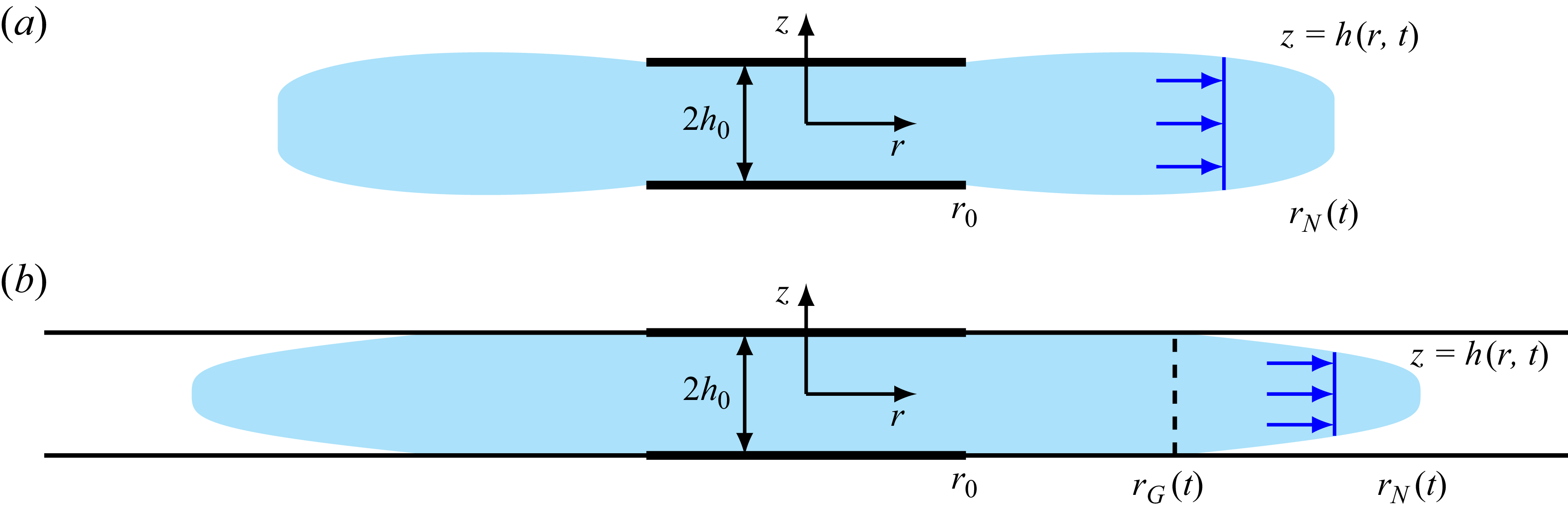


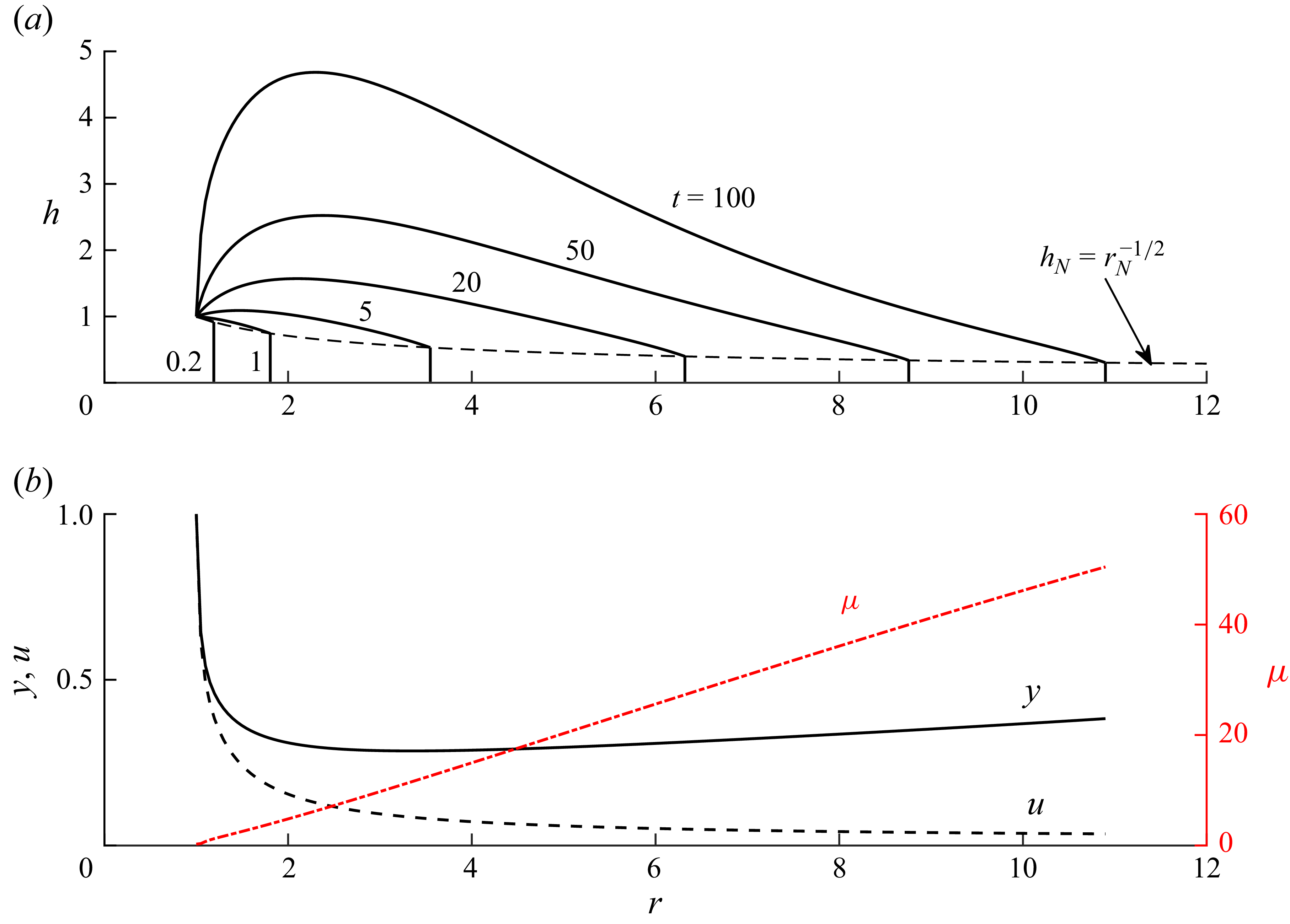


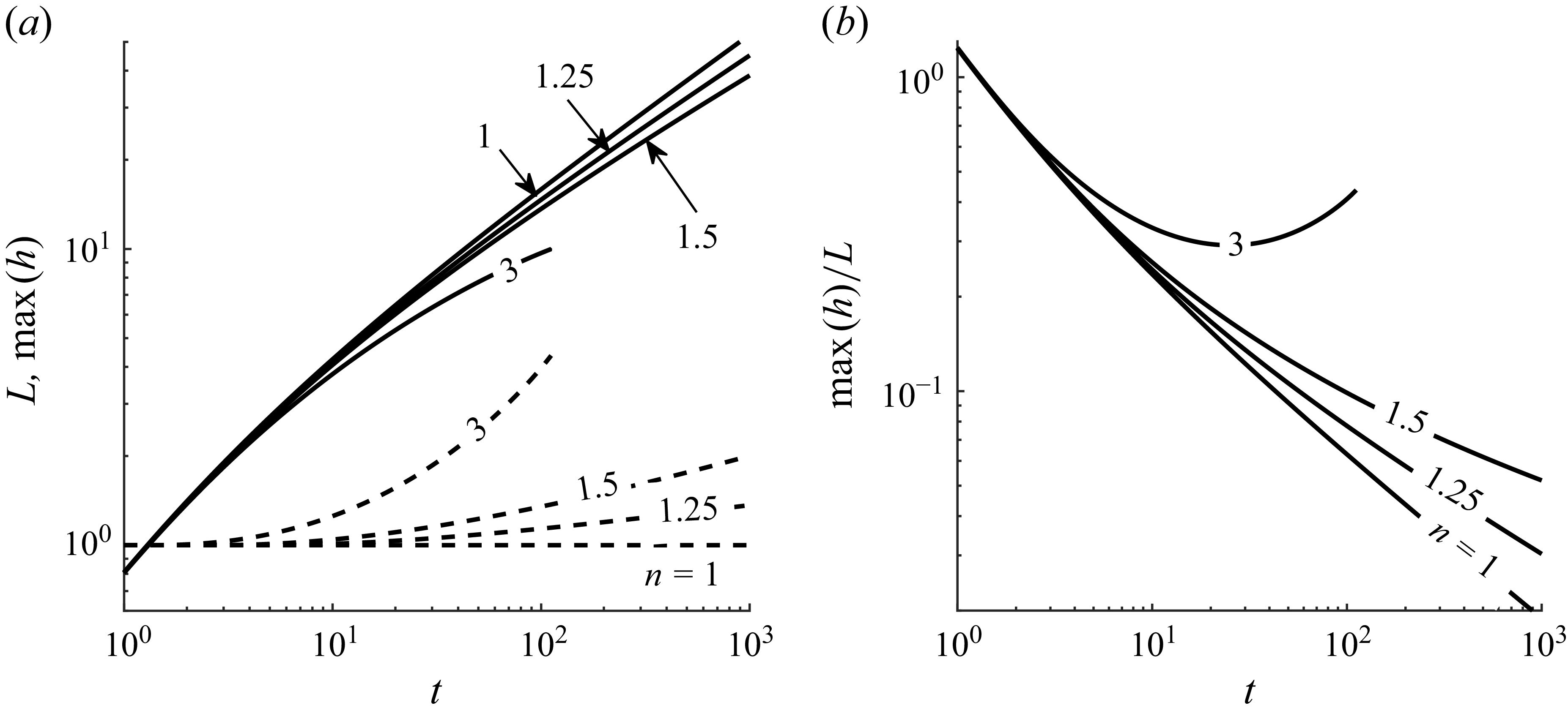


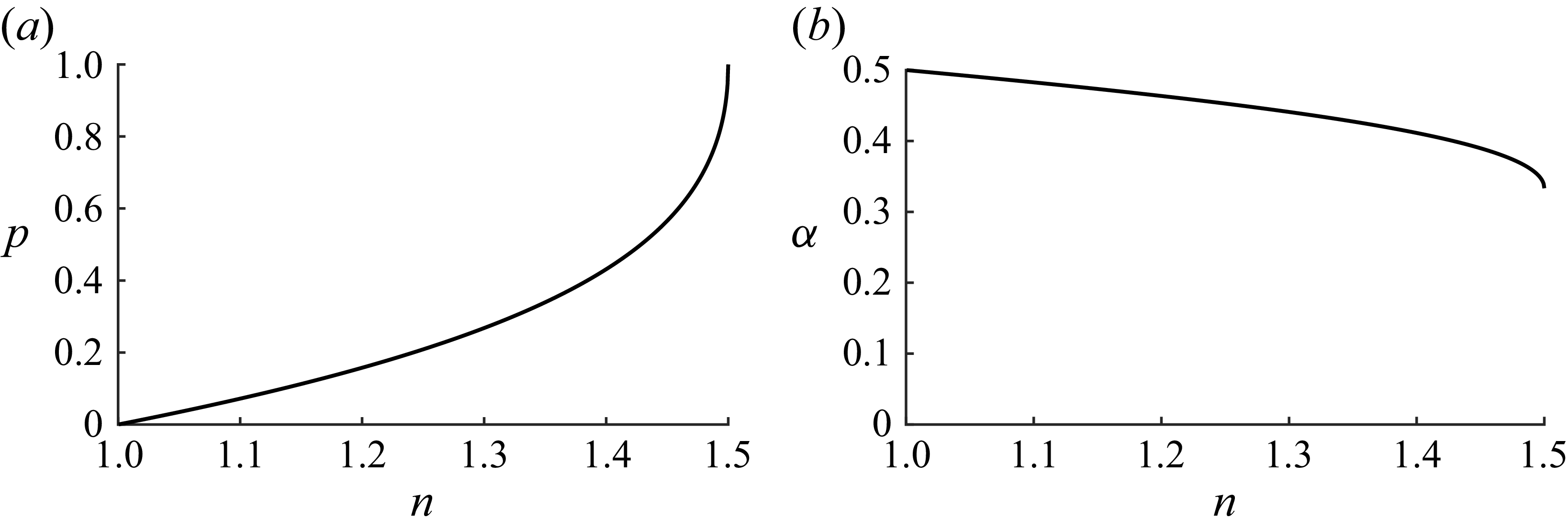


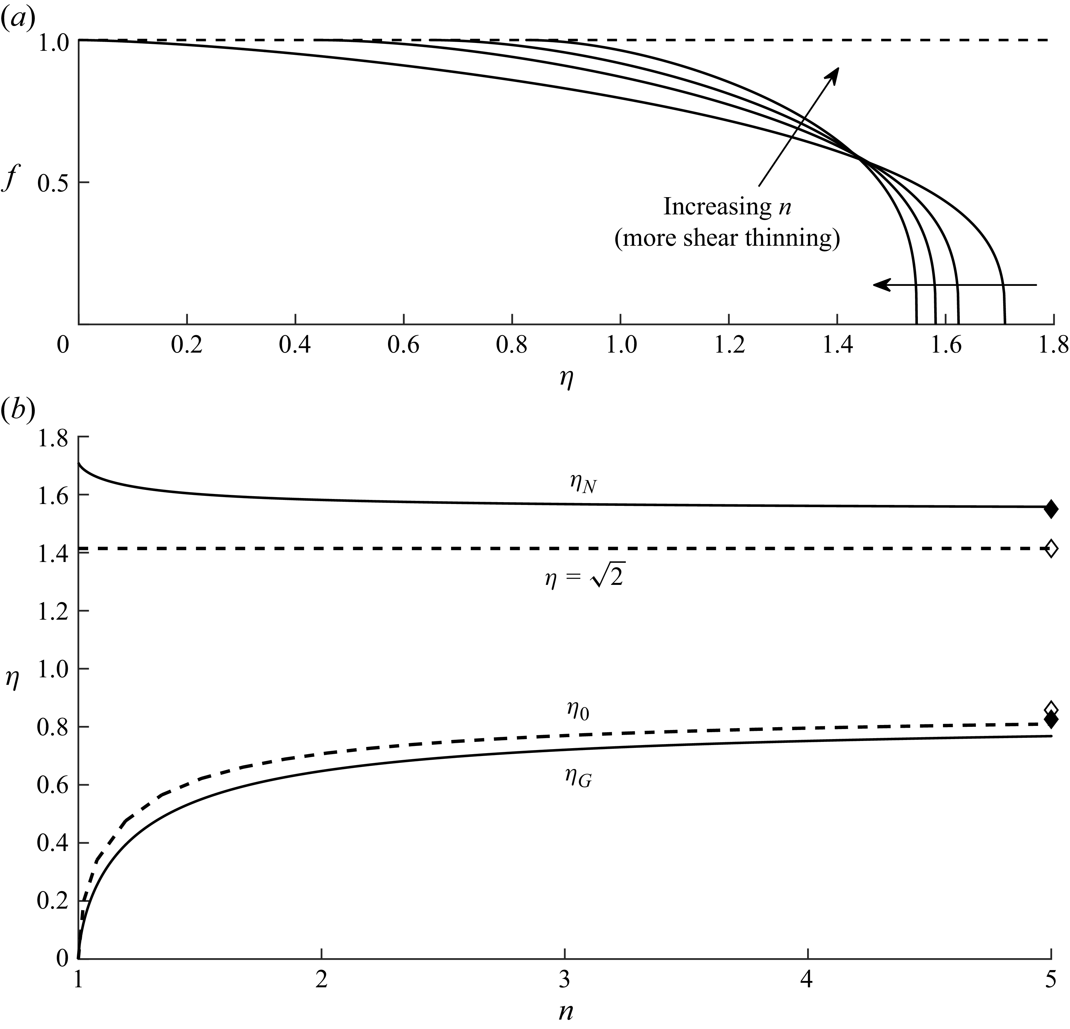


 Open access