


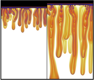





1. Introduction
Carbon dioxide ( ${\rm CO}_{2}$) is the most pervasive greenhouse gas affecting the Earth's climate, and its concentration continues to rise (Arias et al. Reference Arias2021). One of the widely debated geoengineering strategies to decarbonise the atmosphere – and mitigate the impacts of climate change – is geologic carbon sequestration (GCS) within deep brine aquifers (Metz et al. Reference Metz, Davidson, de Coninck, Loos and Meyer2005; Friedmann Reference Friedmann2007). Over the last decade, significant progress has been made in understanding the physics and geochemistry at stake in GCS (Altman et al. Reference Altman2014; Celia et al. Reference Celia, Bachu, Nordbotten and Bandilla2015). It entangles: (i) buoyancy driven flows reaching the uppermost region of deep confined aquifers (stratigraphic trapping); (ii) migration of ${\rm CO}_2$ gas phase and weak ${\rm CO}_2$ dissolution in brines powering convection in the aqueous phase (solubility trapping); (iii) ${\rm CO}_2$ gas phase trapped in the pore space via capillary forces (residual trapping); and (iv) mineral precipitation and fixation of ${\rm CO}_2$ into the solid porous matrix (geochemical trapping) (Metz et al. Reference Metz, Davidson, de Coninck, Loos and Meyer2005; Huppert & Neufeld Reference Huppert and Neufeld2014). However, the complex fluid dynamics of ${\rm CO}_2$ in saline aquifers (hydrodynamic trapping) remains challenging and not yet characterised comprehensively. Advancing in characterising and modelling the fluid dynamics is critical to quantify the irreversible mixing of dissolved ${\rm CO}_{2}$ in brine and thus determine the efficacy and constraints of GCS in deep aquifers.
The fundamentals of  ${\rm CO}_2$ dissolution in brine aquifers have been investigated through analogue models of solutal convection in permeable media, utilising numerical and laboratory experiments (Neufeld et al. Reference Neufeld, Hesse, Riaz, Hallworth, Tchelepi and Huppert2010; Backhaus, Turitsyn & Ecke Reference Backhaus, Turitsyn and Ecke2011; Hidalgo et al. Reference Hidalgo, Fe, Cueto-Felgueroso and Juanes2012; Hewitt, Neufeld & Lister Reference Hewitt, Neufeld and Lister2013; Slim Reference Slim2014; Amooie, Soltanian & Moortgat Reference Amooie, Soltanian and Moortgat2018). Such experiments have used analogue working fluids within porous media and Hele-Shaw cells to mimic and visualise the convective dynamics associated with the supercritical ${\rm CO}_2$ dissolution in brine (Backhaus et al. Reference Backhaus, Turitsyn and Ecke2011; Hewitt et al. Reference Hewitt, Neufeld and Lister2013; MacMinn & Juanes Reference MacMinn and Juanes2013; Slim et al. Reference Slim, Bandi, Miller and Mahadevan2013; Letelier et al. Reference Letelier, Herrera, Mujica and Ortega2016; Alipour, De Paoli & Soldati Reference Alipour, De Paoli and Soldati2020; De Paoli Reference De Paoli2021; De Paoli et al. Reference De Paoli, Perissutti, Marchioli and Soldati2022). Utilised working fluids and environments include methanol and ethylene-glycol (MEG) mixture with water in a cell filled with sand (Neufeld et al. Reference Neufeld, Hesse, Riaz, Hallworth, Tchelepi and Huppert2010; Guo et al. Reference Guo, Sun, Zhao, Li, Liu and Chen2021), MEG doped with sodium iodide and sodium chloride in quasi-two-dimensional (Q-2-D) and three-dimensional (3-D) porous media (Wang et al. Reference Wang, Nakanishi, Hyodo and Suekane2016), and an aqueous solution of propylene glycol (PPG) and deionised water in Hele-Shaw cells (Backhaus et al. Reference Backhaus, Turitsyn and Ecke2011; Hewitt et al. Reference Hewitt, Neufeld and Lister2013).
In the literature, we find two distinctive configurations to investigate solutal convection in porous media: the ‘canonical’ and ‘analogue’ models (Hidalgo et al. Reference Hidalgo, Fe, Cueto-Felgueroso and Juanes2012). In the canonical model, density varies linearly with concentration. In this case, dissolution occurs at the uppermost boundary, whereas a no-flux condition is imposed at the bottom boundary. Conversely, in the analogue model, density varies nonlinearly with concentration. In this case, no-flux conditions are imposed at the top and bottom boundaries. The test fluids used by Neufeld et al. (Reference Neufeld, Hesse, Riaz, Hallworth, Tchelepi and Huppert2010), Backhaus et al. (Reference Backhaus, Turitsyn and Ecke2011) and Hewitt et al. (Reference Hewitt, Neufeld and Lister2013) satisfy a constitutive equation for density of the type  $\rho (S_w) = \rho _{B} + c_{1} S_w + c_{2} S_w^2$, with $S_w$ the mass fraction of the less dense fluid component (see table 1 for symbols' definition). A nonlinear equation for $\rho (S_w)$ enables buoyancy dynamics not supported by linear equations of state, such as ‘cabbeling’, i.e. the formation of an aqueous mixture that is denser than the fluid parcels that gave origin to it (e.g. Groeskamp, Abernathey & Klocker Reference Groeskamp, Abernathey and Klocker2016). Cabbeling, in fact, is the mechanism driving convection, downward mass transport and enhancing irreversible mixing between the analogue working fluids. Here, the fundamental quest is the scaling law linking the non-dimensional mass flux, the Sherwood number $ {{Sh}}$, the Rayleigh number of the system $ {{Ra}}$, and the mean scalar dissipation rate $\vartheta _{scalar}$.
Glossary of general symbols used in the text.

In the canonical model, Amooie et al. (Reference Amooie, Soltanian and Moortgat2018) obtained the sub-linear relationship  $ {{Sh}} \sim {{Ra}}^{0.931}$ for 2-D and 3-D numerical simulations solving the non-Boussinesq Darcy equation with no-flux at the lateral boundaries. This result is valid in the range $1500 \lesssim {{Ra}} \lesssim 135\,000$. The authors remarked that the linear relation $ {{Sh}} \sim { {{Ra}}}$ is attained asymptotically (i.e. for ${ {{Ra}}} \gtrsim 4\times 10^4$). The latter has also been reported in other works using non-Boussinesq/Boussinesq fluids and periodic lateral boundaries (Pau et al. Reference Pau, Bell, Pruess, Almgren, Lijewski and Zhang2010; Slim Reference Slim2014). In the case of laboratory experiments (no-flux conditions at the lateral boundaries), the scaling shows a sub-linear trend of the type $ {{Sh}} \sim { {{Ra}}}^{\alpha }$. In a Q-2-D porous medium, Guo et al. (Reference Guo, Sun, Zhao, Li, Liu and Chen2021) obtained $\alpha = 0.95$, for $400 \lesssim { {{Ra}}} \lesssim 8000$, while in 3-D porous media, Wang et al. (Reference Wang, Nakanishi, Hyodo and Suekane2016) found $\alpha = 0.93$, for $2600 \lesssim { {{Ra}}} \lesssim 16\,000$. These laboratory results show good agreement with numerical results for intermediate ${ {{Ra}}}$. Yet power-law exponents derived from analogue models differ significantly from those obtained from canonical ones. In a Q-2-D porous medium, Neufeld et al. (Reference Neufeld, Hesse, Riaz, Hallworth, Tchelepi and Huppert2010) obtained $ {{Sh}}\sim {{Ra}}^{0.84}$, whereas for Hele-Shaw experiments, Backhaus et al. (Reference Backhaus, Turitsyn and Ecke2011) found $ {{Sh}}\sim {{Ra}}^{0.76}$. These results are consistent with the theoretical scaling law $ {{Sh}}\sim {{Ra}}^{4/5}$ derived by Neufeld et al. (Reference Neufeld, Hesse, Riaz, Hallworth, Tchelepi and Huppert2010), resulting from a balance between vertical advection and horizontal diffusion. Nonetheless, we stress that the nature of the laboratory-scale environment, i.e. porous media and Hele-Shaw, may impact the scaling law's exponent of $ {{Ra}}$. Indeed, we expect that Hele-Shaw cells with larger gaps may lead to smaller exponents (De Paoli, Alipour & Soldati Reference De Paoli, Alipour and Soldati2020). Additionally, discrepancies between scaling laws $ {{Sh}} \sim { {{Ra}}}^{\alpha }$ reported in the literature may also arise from different boundary conditions set in numerical simulations and laboratory experiments.
In this paper, we investigate the irreversible mixing of dissolved  ${\rm CO}_2$ in brine through laboratory-scale numerical experiments utilising a fully miscible two-fluid system. Here, we aim to (i) reconcile apparent discrepancies between scaling laws of the type $ {{Sh}} \sim { {{Ra}}}^{\alpha }$ employing the Hele-Shaw equations (Letelier, Mujica & Ortega Reference Letelier, Mujica and Ortega2019) applied to the analogue model, and (ii) examine the relationship between the non-dimensional mass flux $ {{Sh}}$ and the irreversible mixing controlled by the mean scalar dissipation rate $\vartheta _{scalar}$. We therefore concentrate on finding relationships of the type $ {{Sh}}\sim {{Ra}}^{\alpha (\epsilon )}$, with $\epsilon$ a geometrical scale of the Hele-Shaw cell, to pave the road towards a universal scaling law of the form $ {{Sh}}/\vartheta _{scalar} =b\, {{Ra}}^n$, with $b$ and $n$ independent of $\epsilon$. Such a scaling law may serve for estimating the rate of homogenisation of the dissolved ${\rm CO}_{2}$ in brines.
The paper is organised as follows. In § 2, we introduce the Hele-Shaw model utilised to investigate the problem of cabbeling-powered convection in Q-2-D Hele-Shaw cells as an analogue for the problem of  ${\rm CO}_2$–brine mixing in permeable media. Then in § 3, we derive global conservation equations for the scalar field representing the ${\rm CO}_2$–brine mixture, in order to disentangle the various fluxes involved in the irreversible mixing of the scalar field. The modelling approach is described in § 4, whereas our numerical experiments, benchmarks and scaling results are reported and discussed in § 5. Finally, § 6 summarises our main findings.
2. Hele-Shaw model
We consider a Hele-Shaw domain whose cell gap is  $b$ in the $y^{*}$ coordinate, and whose horizontal length and vertical height are $L$ and $H$ in the $x^{*}$ and $z^{*}$ coordinates, respectively. Conceptually, the Hele-Shaw cell fulfils the relation $b\ll H$ and provides a suitable setting to visualise the fluid dynamics in a transparent, Q-2-D porous-like medium of permeability $K = b^{2}/12$. At the laboratory scale, the cell gaps range from $100\ \mathrm {\mu }{\rm m}$ to 1 mm, while the cell heights can be of the order of $10$ cm. In our model, the cell is filled with an incompressible, density-variable Boussinesq fluid composed of the mixture between two miscible fluids. Both the kinematic viscosity $\nu$ and scalar diffusivity $\kappa$ are assumed to be constant. Figure 1(a) illustrates examples of the density as a function of the water mass fraction (concentration) $S_w$ for aqueous solutions of PPG used to model the ${\rm CO}_2$–brine mixture in laboratory experiments. The density of the fluid mixture is modelled by the nonlinear constitutive relationship
 \begin{equation} \rho^{*}(S_w) = \rho_{B} + f^{*}_{\rho}(S_w) = \rho_{B} + (\rho_{B} - \rho_{A}) \left[ \left(\frac{2\varDelta_w }{1-2\varDelta_w}\right)S_w - \left(\frac{1}{1-2\varDelta_w}\right)S_w^2\right], \end{equation}
with  $f^{*}_{\rho }=\rho ^{*}-\rho _{B}$ the Boussinesq density component, $\rho _{A}$ and $\rho _{B}$ reference densities shown in figure 1(b), and $\varDelta _w$ the concentration at which the fluid density is maximum,
 \begin{equation} \rho^{*}(\varDelta_w) = \rho_{max} = \rho_{B} + \varDelta^2_w\left(\frac{\rho_{B} - \rho_{A}}{1-2\varDelta_w}\right). \end{equation}
Figure 1(b) schematises the boundary and initial conditions of our problem. Initially, the fluid  $A$ of uniform density $\rho _{A}$ is placed over the fluid $B$ of uniform density $\rho _{B}$. The initial interface between fluid $A$ and fluid $B$ is located at height $H_{IB} < H$. Tracking this interface (and its height) is relevant since that is where molecular mixing between both fluids and cabbeling occur.
(a) Density of the aqueous solution of PPG as a function of the water mass fraction (concentration)  $S_w$ and temperature. For a fixed temperature, density satisfies approximately the constitutive relation $\rho (S_w) = \rho _{_B} + c_{1}\, S_w + c_{2}\, S_w^2$ (Sun & Teja Reference Sun and Teja2004; Hewitt et al. Reference Hewitt, Neufeld and Lister2012; Khattab et al. Reference Khattab, Bandarkar, Khoubnasabjafari and Jouyban2017); see (2.1). The parameters $c_{1}$ and $c_{2}$ are constants, and $\rho _{B}$ is the density of the fluid mimicking the brine layer. (b) Conceptual model for the analogue fluid problem in a Hele-Shaw cell, mimicking the ${\rm CO}_{2}$–brine mixing. The cell gap $b$ is much thinner than the cell height $H$, so the 3-D system can be approximated as a Q-2-D geometry, with $u^{*}$ the velocity component in the lateral (horizontal) direction ( $\hat {\boldsymbol {x}}$), and $w^{*}$ the velocity component in the vertical direction ( $\hat {\boldsymbol {z}}$). We impose no-flux ( $\partial S_{w}/\partial z^{*}=0$) and free-slip ( $w^{*}=0$, $\partial u^{*}/\partial z =0$) boundary conditions, at both $z^{*}=0$ and $z^{*}=H$. Initially, a layer of fluid $A$ of density $\rho _{A}$, mimicking the CO $_{2}$ gas phase, lays over a layer of fluid $B$ of density $\rho _{B}>\rho _{A}$ that mimics an aqueous brine layer. Both fluids are fully miscible. The initial concentration $S^{(0)}_{w}(z^{*})$ and density $\rho (S^{(0)}_{w})$ profiles are shown in black and red, respectively. Molecular diffusion between $A$ and $B$ leads to cabbeling, which catalyses the growth of finger-like instabilities and active convection in the region $B$.
$B$.

We consider the following non-dimensional forms of the dimensional variables  ${\boldsymbol {x}}^{*},t^{*},{\boldsymbol {v}}^{*},p^{*},f^{*}_{\rho }$:
 \begin{align} {\boldsymbol{x}} = \frac{{\boldsymbol{x}}^{*}}{H_{IB}}, \quad t = \frac{t^{*}}{H_{IB}/u_c}, \quad \boldsymbol{v} = \frac{{\boldsymbol{v}}^{*}}{u_c}, \quad p = \frac{\tilde{p}^{*}}{p_c} \quad {\rm and}\quad f_{\rho} = \frac{f^{*}_{\rho}}{\Delta\rho_{m}} = 2\,\frac{S_w}{\varDelta_w} - \frac{S_w^2}{\varDelta_w^2}, \end{align}
with  $\Delta \rho _{m} = \rho _{max}-\rho _{B}$ the maximum density difference respect to the deeper fluid $B$,
$B$,  ${\boldsymbol {x}} = x\,\hat {{\boldsymbol {x}}} + z\,\hat {{\boldsymbol {z}}}$ the non-dimensional position, velocity ${\boldsymbol {v}} = u\,\hat {{\boldsymbol {x}}} + w\,\hat {{\boldsymbol {z}}}$ the non-dimensional velocity, $u_{c} = \Delta \rho _{m}\,g K/(\rho _{B}\nu )$ the characteristic velocity, and $p_{c}=\rho _{B}\nu u_{c}H_{IB}/K$ the characteristic pressure. Considering the above geometrical and fluid properties, the non-dimensional 2-D Hele-Shaw equations (Letelier et al. Reference Letelier, Mujica and Ortega2019) are
 \begin{align} \partial_i v_i &= 0 , \end{align}
 \begin{align} \epsilon^{2}\,\frac{ {{Ra}}}{ {{Sc}}}\left(\frac{6}{5}\,\frac{\partial v_i}{\partial t} + \frac{54}{35}\,v_j\,\partial_j v_i\right) &={-}\partial_i p - f_{\rho}(S_w)\,\delta_{iz} - v_i \nonumber\\ &\quad +\epsilon^{2}\,\partial_j^2 v_i + \frac{2}{35}\,\epsilon^{2}\, {{Ra}}\,(v_j\,\partial_j\,S_w)\,\frac{{\rm d}f_{\rho}}{{\rm d}S_w}\,\delta_{iz} , \end{align}
 \begin{align} \frac{\partial S_w}{\partial t} + v_i\,\partial_i S_w &= \frac{1}{ {{Ra}}}\,\partial_i^2 S_w + \frac{2}{35}\,\epsilon^{2}\, {{Ra}}\,\partial_j\left((v_i\,\partial_i S_w)v_j\right), \end{align}
with  ${\rm d}f_{\rho }/{\rm d}S_w = (2/\varDelta _w)(1 - S_w/\varDelta _w)$ the derivative of the Boussinesq density, whereas
 \begin{equation} \epsilon = \frac{\sqrt{K}}{H_{IB}},\quad {{Ra}} = \frac{u_{c}H_{IB}}{\kappa} = \frac{\Delta\rho_{m}\,g K H_{IB}}{\rho_{B}\nu\kappa}\quad {\rm and}\quad {{Sc}} = \frac{\nu}{\kappa} \end{equation}
are the anisotropy ratio, the Rayleigh number for Hele-Shaw cells and the Schmidt number, respectively. The Hele-Shaw equations (2.4) are valid for  $\epsilon \ll 1$, $\epsilon ^{2}\, {{Ra}}\ll 1$ and $ {{Sc}} \geqslant 1$, and they result from averaging the Navier–Stokes equation in the spanwise $\hat {\boldsymbol {y}}$ direction. This averaging procedure of the velocity, pressure and concentration fields in $\hat {\boldsymbol {y}}$ integrates no-slip and no-flux boundary conditions at the vertical walls (Letelier et al. Reference Letelier, Mujica and Ortega2019). Free-slip and no-flux are imposed on the top and bottom boundaries, as shown in figure 1(b). We consider two scenarios for the lateral boundaries, no-flux and free-slip conditions (closed system), and periodic boundary conditions. For $\epsilon \rightarrow 0$, the model (2.4) reduces to the Darcy equation coupled with the advection–diffusion model (e.g. Hewitt, Neufeld & Lister Reference Hewitt, Neufeld and Lister2012). Notice that in nature, the Schmidt number of ${\rm CO}_2$–brine mixtures is about $10^{3}$, while for analogue fluids utilised in laboratory experiments, $10\leqslant {{Sc}} \leqslant 100$. Moreover, regardless of the flow regime (Darcian or Hele-Shaw), we note that greater Schmidt numbers will weaken the inertial effects in the momentum balance (2.4b), making mechanical dispersion the most relevant term affecting convective dynamics beyond the Darcian regime (Liang et al. Reference Liang, Wen, Hesse and DiCarlo2018).
3. Global conservation equations
We study global quantities associated with mass transfer and mixing in the time-dependent domain  $\varOmega _c(t)$ sketched in figure 1(b). The (dimensional) averaged height $h^{*}(t)$ defines the upper boundary of $\varOmega _c$, with $h^{*}(t=0) = H_{IB}$. For $t>0$, the definition and computation of $h^{*}$ are somewhat arbitrary and depend on authors’ criteria. Nevertheless, the global conservation equations introduced in this section are independent of the chosen criteria; our definition of $h^{*}$ and method adopted to compute it are introduced in § 3.1.
Henceforth, we express the ‘mean’ of a physical variable  $f(t,{\boldsymbol {x}})$ through the lateral ( $\hat {\boldsymbol {x}}$ direction) and domain integrals as
 \begin{equation} \langle f\rangle_{\ell} (t,z) = \frac{1}{\mathscr{L}}\int_{0}^{\mathscr{L}} f(t,{\boldsymbol{x}})\,{\rm d}\kern 0.06em x \quad {\rm and}\quad \langle f\rangle_{\upsilon}(t) = \int_{0}^{h(t)}\langle f\rangle_{\ell}(t,z)\,{\rm d}z, \end{equation}
respectively, with  $\mathscr {L}=L/H_{IB}$ the effective cell aspect ratio, and $h(t)=h^{*}(t)/H_{IB}$ the non-dimensional averaged height. Likewise, we express the time average of a function $f(t)$ over a window of size $\tau$ as
 \begin{equation} \langle f\rangle_{\tau} = \frac{1}{\tau}\int_{t}^{t+\tau}\, f(\tilde{t})\,{\rm d}\tilde{t}. \end{equation}
3.1. Interface detection and first conservation equation
For an arbitrary 2-D ‘control volume’  $\varOmega (t)$, the Reynolds transport theorem establishes that the rate of change of a non-dimensional quantity $\int _{\varOmega (t)} f(t,x,z)\,{\rm d}\kern 0.06em x\,{\rm d}z$ is given by
 \begin{equation} \frac{{\rm d}}{{\rm d}t}\left[\int_{\varOmega(t)} f\,{\rm d}\kern 0.06em x\,{\rm d}z\right] = \int_{\varOmega(t)} \frac{\partial f}{\partial t}\,{\rm d}\kern 0.06em x\,{\rm d}z + \oint_{\partial \varOmega(t)} fv_in_i\,{\rm d}s , \end{equation}
with  $\partial \varOmega$ the boundary of the ‘volume’ $\varOmega$, ${\rm d}s$ the infinitesimal ‘length’ of $\partial \varOmega$, and $v_i$ the $i$th component of the (non-dimensional) velocity at $\partial \varOmega$. Let us now consider $f = S_w$. Applying (3.3) over a specific volume $\varOmega _c$ and normalising by $\mathscr {L}$, we obtain
 \begin{equation} \frac{1}{\mathscr{L}}\int_{\varOmega_c(t)} \frac{\partial S_w}{\partial t}\,{\rm d}\kern 0.06em x\,{\rm d}z = \frac{1}{\mathscr{L}}\,\frac{\rm d}{{\rm d}t}\left[\int_{\varOmega_c(t)} S_w\,{\rm d}\kern 0.06em x\,{\rm d}z\right] - \frac{1}{\mathscr{L}}\left.\int_0^{\mathscr{L}} w_{h}S_w\right|_{z=h}{\rm d}\kern 0.06em x, \end{equation}
where  $w_{h}$ corresponds to the rate of change over time of $h(t)$. Using (3.1a,b) and assuming that $w_{h}$ is a constant (Neufeld et al. Reference Neufeld, Hesse, Riaz, Hallworth, Tchelepi and Huppert2010), (3.4) can be written compactly as
 \begin{equation} \left\langle \frac{\partial S_w}{\partial t} \right\rangle_{\upsilon} = \left.\frac{{\rm d}}{{\rm d}t}\langle S_w \rangle_{\upsilon} - w_{h}\,\langle S_w \rangle_{\ell}\right|_{z=h} , \end{equation}
with  $\langle S_w \rangle _{\ell }|_{z=h}$ the horizontal average of $S_w$ evaluated at $h(t)$. Thus the transport equation governing the water mass fraction over the domain $\varOmega _c$ is obtained by integrating (2.4c), i.e.
 \begin{align} \int_{\varOmega_c} \frac{\partial S_w}{\partial t}\,{\rm d}\kern 0.06em x\,{\rm d}z + \int_0^{\mathscr{L}} \left.\left[S_w - \frac{2}{35}\,\epsilon^{2}\, {{Ra}}\left(v_i\,\partial_i S_w\right) \right] w\right|_{z=h}{\rm d}x = \frac{1}{ {{Ra}}}\int_0^{\mathscr{L}}\left.\frac{\partial S_w}{\partial z}\right|_{z=h}{\rm d}x . \end{align}
Using (3.5) and the mean quantities defined in (3.1a,b), (3.6) can be contracted to
 \begin{equation} {{Ra}}\,\frac{{\rm d}}{{\rm d}t}\langle S_w \rangle_{\upsilon} ={-} \mathcal{F}_{ad} +\left. {{Ra}}\, w_{h}\,\langle S_w \rangle_{\ell}\right|_{z=h} + \left.\frac{\partial \langle S_w\rangle_{\ell}}{\partial z}\right|_{z=h} , \end{equation}
with  $\mathcal {F}_{ad}$ the advective–dispersive flux defined as
 \begin{equation} \mathcal{F}_{ad} = \left. {{Ra}}\,\langle S_w w \rangle_{\ell}\right|_{z=h} - \tfrac{2}{35}\epsilon^2\, {{Ra}}^{2}\,\langle w\,\partial_i(S_w v_i) \rangle_{\ell}|_{z=h}. \end{equation}
 Previous authors have chosen different criteria to define and compute  $h(t)$. Neufeld et al. (Reference Neufeld, Hesse, Riaz, Hallworth, Tchelepi and Huppert2010) studied the laterally averaged concentration profile and used the ‘flat’ interfacial region – which propagated upwards at a constant speed – to estimate an advective mass flux. In contrast, Hewitt et al. (Reference Hewitt, Neufeld and Lister2013) defined $h$ as the averaged interfacial height where $\langle S_w\rangle _{\ell }|_{z=h} = \varDelta _w$, i.e. the position at which the horizontally averaged density is maximum. The ‘interface’, with height $h_{int}(t,x)$, is defined as the contour satisfying $S_w(x,z=h_{int}(t,x)) = \varDelta _w$. This locus is geometrically complex and not flat (see figure 2b) (e.g. Hidalgo et al. Reference Hidalgo, Dentz, Cabeza and Carrera2015). Another alternative is to define $h$ as the solution of the equation $\mathcal {F}_{ad} = 0$ in (3.8). The latter implies that the mass transfer at $h(t)$ is governed by molecular diffusion $\partial _z\langle S_w\rangle _{\ell }|_{z=h}$ and the flux due to the rejection at constant velocity $w_{h}$ of the contour drawn by $h$. The criterion above to determine $h(t)$ is feasible via numerical simulations. However, its application to laboratory experiments is challenging owing to the necessity to resolve the velocity and scalar fields simultaneously.
(a) Spatiotemporal evolution of the scalar field  $S_{w}$ modelling the mixing of the initial two-fluid system in a Hele-Shaw cell mimicking the ${\rm CO}_{2}$–brine mixture. The plotted area highlights the transition between the upper stable layer and the deeper convective layer. (b) Spatiotemporal evolution of the isoscalar $S_{w}=\varDelta _{w}$ drawn with the dimensional height (‘interface’) $h^{*}_{int}(t^{*},x^{*})$, defining the locus of the maximum density (Hewitt et al. Reference Hewitt, Neufeld and Lister2013). This locus is not flat. (c) Spatiotemporal evolution of the isoscalar $S_{w}=2\varDelta _{w}$ drawn by the height $h^{*}_{iso}(t^{*},x^{*})$, found above the ‘interface’. This locus is substantially flatter in comparison to (b), allowing us to define a robust averaged height $h(t)$ (in its non-dimensional form).

Here, we define  $h(t)$ so that its computation via laboratory or numerical experiments is straightforward. First, we note that $\rho (S_w = 2\varDelta _w) = \rho _{B}$ corresponds to the density of the initial bottom layer (fluid $B$). Let us introduce $h_{iso}(t,x)$ as the contour satisfying $S_w(x,h_{iso}(t,x)) = 2\varDelta _w$. This locus is substantially flatter (quasi-flat) than the case of the ‘interface’ $h_{int}(t,x)$ (compare figures 2b,c). The latter allows us to define the averaged height $h(t)$ robustly as the solution of $\langle S_w\rangle _{\ell }|_{z=h} = 2\varDelta _w$. This $h$ splits the Hele-Shaw cell into two time-dependent rectangular domains, a convective region $\varOmega _c(t)$, and a stable region $\varOmega _s(t)$, as in figure 1(b).
A global description of the problem requires studying the convective dynamics of the ‘free-falling’ plumes, i.e. from the state in which the downward plumes are sufficiently spaced from local mergers beneath the interface until the first megaplume reaches the bottom of the Hele-Shaw cell. This regime is known as the constant flux (Slim Reference Slim2014) or late convection (Amooie et al. Reference Amooie, Soltanian and Moortgat2018). The time window  $\tau$ that captures the stage of free-falling convective plumes is denoted as the integral time scale. Over this time scale, physical quantities such as ${\rm d}\langle S_w \rangle _{\upsilon }/{\rm d}t$, ${\rm d}h/{\rm d}t$ and $\partial \langle S_w \rangle _{\ell }/{\partial z}|_{z=h}$ have a statistically stationary behaviour (see § 5). Therefore, applying the time average defined in (3.2) and the ‘normalised’ scalar field $\varphi = S_w/2\varDelta _w$, (3.7) can be written as
 \begin{equation} \left\langle {{Ra}}\,\frac{{\rm d}}{{\rm d}t}\langle \varphi \rangle_{\upsilon} \right\rangle_{\tau} ={-} \frac{1}{2\varDelta_w}\,\langle \mathcal{F}_{ad} \rangle_{\tau} + {{Ra}}\, w_{h} + \left\langle \left.\frac{\partial \langle \varphi\rangle_{\ell}}{\partial z}\right|_{z=h} \right\rangle_{\tau}. \end{equation}
Equation (3.9) denotes the first conservation law utilised to characterise the mass transfer rate between the fluid  $A$ (
$A$ ( ${\rm CO}_2$ gas phase) and fluid $B$ (aqueous brine layer). Within the integral time scale, $O(\mathcal {F}_{ad}/(2\varDelta _{w})) \ll O({ {{Ra}}}\,w_{h}), \langle \partial \langle \varphi \rangle _{\ell }/\partial z|_{z=h} \rangle _{\tau }$, i.e. the contribution of $\mathcal {F}_{ad}$ can be ignored. The latter is shown in the Appendix, figure 10. Interestingly, each of the remainder terms in (3.9) can be interpreted as a non-dimensional parameter. The time average of the mean scalar rate of change is defined as the ‘global’ Sherwood number
 \begin{equation} {{Sh}}_{\varphi} = \left\langle {{Ra}}\,\frac{{\rm d}}{{\rm d}t}\langle \varphi \rangle_{\upsilon} \right\rangle_{\tau}. \end{equation}
De Paoli et al. (Reference De Paoli, Alipour and Soldati2020) used a similar version of (3.10) to construct the scaling law associated with the dissolution rate of potassium permanganate,  ${\rm KMnO}_4$, into water in a Hele-Shaw cell, whereas Guo et al. (Reference Guo, Sun, Zhao, Li, Liu and Chen2021) adopted (3.10) to estimate the dissolution rate of MEG in pure ${\rm H}_{2}{\rm O}$ within a porous medium. On the other hand, the ‘local’ Sherwood number, defined as
 \begin{equation} {{Sh}} = {{Ra}}\, w_{h}, \end{equation}
is based on the rate at which the contour  $h_{iso}(t,x)$ expands vertically in response to the mass exchange. Neufeld et al. (Reference Neufeld, Hesse, Riaz, Hallworth, Tchelepi and Huppert2010) used a similar version of $ {{Sh}}$ to construct the scaling law associated with the dissolution of MEG into ${\rm H}_{2}{\rm O}$ in a porous medium. In addition, the term $\langle \partial \langle \varphi \rangle _{\upsilon }/\partial z|_{z=h}\rangle _{\tau }$ in (3.9) can be interpreted as a solutal Nusselt number,
 \begin{equation} {{Nu}}_{\varphi} = \left\langle \left.\frac{\partial \langle \varphi\rangle_{\ell}}{\partial z}\right|_{z=h} \right\rangle_{\tau}, \end{equation}
which is analogous to the Nusselt number employed to quantify the global heat transfer rate due to thermal convection in porous media (Hewitt et al. Reference Hewitt, Neufeld and Lister2012) and Hele-Shaw cells (Letelier et al. Reference Letelier, Mujica and Ortega2019).
If the control volume  $\varOmega _c$ is extended over the whole domain (see figure 1b), then the conservation equation for $\langle \varphi \rangle$ simplifies to
 \begin{equation} \frac{{\rm d}}{{\rm d}t}\langle\varphi \rangle = 0 , \quad \text{with} \langle \varphi \rangle = \frac{1}{\mathscr{L}}\int_0^{\mathscr{H}} \int_0^{\mathscr{L}} \varphi(t,x,z)\,{\rm d}\kern 0.06em x\,{\rm d}z, \end{equation}
where  $\mathscr {H} = H/H_{IB}$. The mass budget in (3.13) shows the relevance of using a time-dependent control volume $\varOmega _c(t)$ to disentangle the physics and quantify the mass transfer between the quiescent upper layer and the deeper convective mixing layer.
3.2. Second conservation equation
We investigate the irreversible mixing in the system through the evolution of the scalar variance  $\varphi ^2$. The equation governing the rate of change of $\varphi ^2$ can be derived by multiplying (2.4c) by $S_w$. Averaging the resulting equation over the domain $\varOmega _c$ and relocating $ {{Ra}}$, the evolution equation for $\langle \varphi ^2/2\rangle _{\upsilon }$ is given by
 \begin{equation} {{Ra}}\,\frac{{\rm d}}{{\rm d}t}\left\langle \frac{1}{2}\,\varphi^2 \right\rangle_{\upsilon} ={-} \mathcal{F}_{var} + {{Ra}}\,w_{h}\left\langle \left.\frac{1}{2}\,\varphi^2 \right\rangle_{\ell}\right|_{z=h} + \frac{\partial}{\partial z}\left\langle \left.\frac{1}{2}\,\varphi^2 \right\rangle_{\ell}\right|_{z=h} - {{Ra}}\,\langle \varPhi^{(\epsilon)}_{scalar} \rangle_{\upsilon}, \end{equation}
with  $\mathcal {F}_{var}$ the variance flux, and $\varPhi ^{(\epsilon )}_{scalar}$ the scalar dissipation rate, defined as
 $$\begin{gather} \mathcal{F}_{var} = {{Ra}} \left\langle \left.\frac{1}{2}\,\varphi^2 w \right\rangle_{\ell}\right|_{z=h} - \frac{2}{35}\,\epsilon^2\, {{Ra}}^{2}\left.\left\langle w\, \partial_i\left(\frac{1}{2}\,\varphi^2 v_i\right) \right\rangle_{\ell}\right|_{z=h}, \end{gather}$$
 $$\begin{gather}\varPhi^{(\epsilon)}_{scalar} = \frac{1}{ {{Ra}}}\,(\partial_i \varphi)^2 + \frac{2}{35}\,\epsilon^2\, {{Ra}}\left(\partial_i(\varphi v_i)\right)^2. \end{gather}$$
 The physics of  $\langle \varPhi ^{(\epsilon )}_{scalar} \rangle _{\upsilon }$ can be interpreted straightforwardly by extending the control volume to the entire Hele-Shaw cell. Applying the domain average defined in (3.13) and the adiabatic boundary conditions for the Hele-Shaw cell, (3.14) reduces to
 \begin{equation} {{Ra}}\,\frac{{\rm d}}{{\rm d}t}\left\langle \frac{1}{2}\,\varphi^2 \right\rangle ={-} {{Ra}}\,\langle \varPhi^{(\epsilon)}_{scalar} \rangle. \end{equation}
The right-hand side term in (3.17) is a negative-definite quantity that determines the global decay rate of the scalar variance (Ulloa & Letelier Reference Ulloa and Letelier2022). As a result,  $\langle \frac {1}{2}\varphi ^2 \rangle (t)$ is a monotonically decreasing function in time owing to irreversible mixing and homogenisation of the scalar $\varphi$ (i.e. $S_{w}$) inside the fluid environment. If the rate of change of the mean scalar variance $\langle \varphi ^{2}/2 \rangle _{\upsilon }$ is statistically constant over the integral time scale $\tau$, then we can characterise the quasi-steady fluxes governing the scalar variance transport and irreversible mixing in $\varOmega _{c}$ as
 \begin{align}
{{Ra}}\left\langle \frac{{\rm d}}{{\rm
d}t}\left\langle \frac{1}{2}\,\varphi^2
\right\rangle_{\upsilon}\right\rangle_{\tau} &={-}
\langle\mathcal{F}_{var}\rangle_{\tau}
+ {{Ra}}\left\langle w_{h}\left.\left\langle
\frac{1}{2}\,\varphi^2
\right\rangle_{\ell}\right|_{z=h}\right\rangle_{\tau}\nonumber\\
&\quad + \left\langle\frac{\partial}{\partial z}\left.\left\langle
\frac{1}{2}\,\varphi^2
\right\rangle_{\ell}\right|_{z=h}\right\rangle_{\tau} -
{{Ra}}\,\vartheta_{scalar},
\end{align}
\begin{align}
{{Ra}}\left\langle \frac{{\rm d}}{{\rm
d}t}\left\langle \frac{1}{2}\,\varphi^2
\right\rangle_{\upsilon}\right\rangle_{\tau} &={-}
\langle\mathcal{F}_{var}\rangle_{\tau}
+ {{Ra}}\left\langle w_{h}\left.\left\langle
\frac{1}{2}\,\varphi^2
\right\rangle_{\ell}\right|_{z=h}\right\rangle_{\tau}\nonumber\\
&\quad + \left\langle\frac{\partial}{\partial z}\left.\left\langle
\frac{1}{2}\,\varphi^2
\right\rangle_{\ell}\right|_{z=h}\right\rangle_{\tau} -
{{Ra}}\,\vartheta_{scalar},
\end{align}
with  $\vartheta _{scalar} = \langle \langle \varPhi ^{(\epsilon )}_{scalar}\rangle _{\upsilon }\rangle _{\tau }$ the mean scalar dissipation rate. Equation (3.18) corresponds to the second conservation law of the fluid environment investigated here.
4. Method: numerical experiments
We performed numerical experiments using the spectral solver flow $\_$solve (Winters Reference Winters and de la Fuente2012), which has been applied successfully to resolve buoyancy-driven flows in Hele-Shaw cells (Letelier et al. Reference Letelier, Mujica and Ortega2019; Ulloa & Letelier Reference Ulloa and Letelier2022). The dynamical variables in (2.4a)–(2.4c) were expanded by means of trigonometric basis functions over the Hele-Shaw computational domain, and integrated in time using a third-order Adams–Bashforth scheme for advective/buoyant terms and the implicit fourth-order Adams–Moulton method for diffusive scheme.
The problem of irreversible mixing between dissolved CO $_{2}$ and brine does not admit a base state solution. The initial condition for the scalar field is given by
 \begin{equation} S^{(0)}_w(z) = 1 - \frac{H_{IB}}{H} - \frac{2}{\rm \pi} \sum_{n=1}^{N} \frac{1}{n} \sin\left(\frac{n {\rm \pi}H_{IB}}{H}\right) \cos\left(\frac{n {\rm \pi}z}{H}\right) \exp({-n^2 {\rm \pi}^2 \bar{t}}), \quad \bar{t} \ll 1, \end{equation}
whereas the velocity components satisfy  $(u,w)|_{t=0} = (0,0)$. To fulfil the boundary conditions defined in figure 1(b), we expanded $u\sim f_u(n_x,x)\cos (n_z{\rm \pi} z)$, $w\sim f_w(n_x,x) \sin (n_z{\rm \pi} z)$, $p\sim f_p(n_x,x)\cos (n_z{\rm \pi} z)$ and $S_{w}\sim f_s(n_x,x)\cos (n_z {\rm \pi}z)$, with $n_x$ and $n_z$ the number of grid points in $x$ and $z$ coordinates, respectively. The functions $f_{\beta }$, with $\beta \in \{u,w,p,s\}$, depend on lateral boundary conditions. For no-flux, free-slip lateral conditions, $f_u = \sin (n_x{\rm \pi} x)$ and $f_w = f_p = f_s = \cos (n_x{\rm \pi} x)$. On the other hand, for periodic lateral conditions, $f_u=f_w=f_p=f_s=\exp (n_x{\rm \pi} x)$. The effective cell aspect ratio was $\mathscr {L} = L/H_{IB} = 2/3$, while the entire domain aspect ratio was $L/H = 1/2$.
For no-flux, free-slip lateral conditions, the dimensional spatial resolutions in  $x$ and $z$ were $\varDelta _{x}^{*} = L/(n_{x}-1)$ and $\varDelta _{z}^{*} = H/(n_{z}-1)$, respectively, such that $\varDelta = \Delta^{*}_{x}=\Delta^{*}_{z}$. Likewise, for periodic lateral conditions, we keep the homogeneity of the grid $\varDelta$, but $\varDelta _{x}^{*} = L/n_{x}$ because the point $x(n_x)$ is not stored explicitly in flow $\_$solve. The resolution $\varDelta$ was chosen to resolve the spectral Batchelor scale $\varDelta \leqslant {\rm \pi}\varDelta _b$ (Grötzbach Reference Grötzbach1983), with $\varDelta _b = (\nu ^3/\varepsilon \, {{Sc}}^2)^{1/4}$ the Batchelor length scale, and $\varepsilon \sim \nu u_c^{2}/K$ the scale of the kinetic energy dissipation rate. The time step met the Courant–Friedrichs–Lewy (CFL) condition of the numerical scheme, ${\rm CFL}\leqslant 0.02$, for both velocity components (Letelier et al. Reference Letelier, Mujica and Ortega2019).
The horizontal average of a function  $f_i = f(x_i)$ over $n_{x}$ grid points was based on a cubic spline interpolation of $f$ in a three times denser grid, with $m_x = 3n_x$ points. The interpolated function $f^{new}_{j}$, with $j = 1,\ldots,m_x$, was integrated using the composite Simpson's rule. We used the same procedure for the domain average of the $z$-dependent function. Numerical derivatives were computed using a spectral approach based on sine and cosine transforms, depending on the boundary conditions.
Our numerical experiments encompassed  $10^{3} \leqslant {{Ra}} \leqslant 3\times 10^{4}$, with $ {{Sc}} = 10$, and three values of the anisotropy ratio, $\epsilon =5\times 10^{-4}$, $\epsilon =3\times 10^{-3}$ and $\epsilon =5\times 10^{-3}$. The simulations were run in high-performance computers using up to 80 cores over four advective time scales, defined as $H^2_{IB}/(\kappa \, {{Ra}})$. This simulation time was enough to resolve the full transition from the onset of convection to the instant that megaplumes reached the bottom boundary of the Hele-Shaw cell. Table 2 summarises the experimental set and numerical results for the non-dimensional mass flux parameters.
Summary of non-dimensional experimental parameters and results. The experimental set is conformed by three subsets, each of them characterised by single anisotropy ratio  $\epsilon$ and a range of Rayleigh $ {{Ra}}$ and Péclet $Pe = \epsilon \, {{Ra}}$ numbers. The Schmidt number $ {{Sc}}=10$ was kept constant for all our experiments. Here, $ {{Sh}}_{\varphi }$ is the Sherwood number introduced in (3.11), and $ {{Sh}}^{(m)}_{\varphi }=\epsilon \, {{Sh}}_{\varphi }$ is the modified Sherwood number computed from the numerical results.

5. Results and discussion
5.1. The adiabatic analogue model in the Darcian regime
In order to have a robust benchmark, we conducted a first set of numerical experiments adopting the laboratory scales employed by Neufeld et al. (Reference Neufeld, Hesse, Riaz, Hallworth, Tchelepi and Huppert2010), i.e. an analogue model with no-flux boundary conditions. The cell dimensions used by Neufeld et al. (Reference Neufeld, Hesse, Riaz, Hallworth, Tchelepi and Huppert2010) were  $b=1.4$ cm, $L = 40$ cm and $H = 80$ cm, and it was filled with a granular material. The initial position of the interface was $H_{IB} = 60$ cm, so the effective cell aspect ratio was $\mathscr {L} = L/H_{IB}= 2/3$. Here, we modelled the porous medium used in Neufeld et al. (Reference Neufeld, Hesse, Riaz, Hallworth, Tchelepi and Huppert2010) by adopting a small anisotropy ratio such that Hele-Shaw equations (and Hele-Shaw cells) recover the Darcian regime. The latter regime is achieved for $\epsilon = 5\times 10^{-4}$. Notice that a fully analogue anisotropy ratio for the Neufeld et al. (Reference Neufeld, Hesse, Riaz, Hallworth, Tchelepi and Huppert2010) experiments should be one order of magnitude smaller. However, for such a tiny value of $\epsilon$, numerical experiments become considerably more expensive while not providing new results. For the adopted value of $\epsilon$, and considering cell height $H=80$ cm, an experimental Hele-Shaw cell must have cell gap $b=\sqrt {12}\,\epsilon H\approx 1.5$ mm and fulfil $\epsilon ^{2}\, {{Ra}}\ll 1$ (Letelier et al. Reference Letelier, Mujica and Ortega2019; De Paoli et al. Reference De Paoli, Alipour and Soldati2020) – i.e. the Rayleigh number should be no larger than $4\times 10^5$.
Figure 3 shows the spatiotemporal evolution of the mass fraction  $S_w$ and the scalar dissipation rate $\varPhi ^{(\epsilon )}_{scalar}$ to illustrate the solutal convection and mixing in the two-fluid system. The non-dimensional parameters of the numerical experiment are $\varDelta _w=0.3$, ${ {{Sc}} = 10}$ and $ {{Ra}} = 10^{4}$. Figure 3(a) encompasses a time window that captures the emergence of instabilities in the early convection or flux growth regime (Slim Reference Slim2014; Amooie et al. Reference Amooie, Soltanian and Moortgat2018) and snapshots illustrating the late convection or constant flux regime, until the first megaplume reaches the bottom boundary. After the onset of convection, lateral diffusion leads to a continuous process of coalescence, where two or more plumes merge, creating megaplumes that enhance downward mass transfer. Simultaneously, figure 3(b) shows the scalar dissipation rate $\varPhi ^{(\epsilon )}_{scalar}$, highlighting that vigorous mixing occurs at the diffusive layer and edges of convective plumes. The latter demonstrates that horizontal diffusion is an active process in the convective region, as posited by Neufeld et al. (Reference Neufeld, Hesse, Riaz, Hallworth, Tchelepi and Huppert2010). Additionally, figure 3 shows the slow yet pervasive interface upward displacement caused in response to the continuous bloom of protoplumes.
Mass fraction  $S_w$ and scalar dissipation rate $\varPhi ^{(\epsilon )}_{scalar}$ for the mixing of the initial two-fluid system in a Hele-Shaw cell, with $\mathscr {L} = L/H_{IB} = 2/3$, $L/H = 1/2$, $\varDelta _w = 0.3$, $ {{Sc}} = 10$, $ {{Ra}} = 10^{4}$ and $\epsilon = 5\times 10^{-4}$. Slides are shown for different times. The advective time scale is defined as $t_{adv} = H_{IB}/u_c$.

Figure 4 shows time series for the mean dissipation rate of the scalar variance,  $\langle \varPhi ^{(\epsilon )}_{scalar}\rangle _{\upsilon }$, for $\epsilon = 5\times 10^{-4}$ and $ {{Ra}} = 3000$, $10\,000$ and $30\,000$. During the onset of convection due to cabbeling and after the diffusive regime, $\langle \varPhi ^{(\epsilon )}_{scalar}\rangle _{\upsilon }$ shows a transient behaviour characterised by a sharp and large amplitude peak, associated with the flux growth regime. This first peak is followed by a relaxation phase associated with the merging regime. The mergers between primary plumes continue, but the system reaches a quasi-steady rate of decay of the scalar variance $\varphi ^{2}$ within the volume $\varOmega _{c}(t)$, governed by the second conservation equation (3.14) – the late convection regime. This result allows us to define an ad hoc integral time scale $\tau$ that characterises the period over which $\langle \varPhi ^{(\epsilon )}_{scalar}\rangle _{\upsilon }$ is statistically steady, until the first megaplume reaches the bottom. Note that at the quasi-steady state, the mean dissipation rate of the scalar variance decreases as the Rayleigh number increases, showing a functional dependence between $\langle \varPhi ^{(\epsilon )}_{scalar}\rangle _{\upsilon }$ and $ {{Ra}}$.
Time series of the mean scalar dissipation rate  $\langle \varPhi ^{(\epsilon )}_{scalar}\rangle _{\upsilon }$ for $\epsilon =5\times 10^{-4}$ and $3\times 10^{3}\leqslant {{Ra}} \leqslant 3\times 10^{4}$.

Figure 5 shows time series of the physical quantities governing the first conservation equation (3.9), for two numerical experiments, with  $\epsilon =5\times 10^{-4}$, and $ {{Ra}}=10^{4}$ and $ {{Ra}}=3\times 10^{4}$, respectively. Each panel highlights the integral time scale $\tau$. The evolution in time of the averaged height $h(t)$ is shown in figures 5(a,d). The results illustrate that $h(t)$ grows linearly, implying that the convective region $B$ expands vertically at a constant rate. The latter is remarkable since it indicates that global quantities and boundary fluxes, such as ${\rm d}\langle \varphi \rangle _{\upsilon }/{\rm d}t$ and $(\partial \langle \varphi \rangle _{\ell }/\partial z) |_{z=h}$, reach statistically steady states over $\tau$, shown in figures 5(b,e) and 5(c, f), respectively. Hence we can rigorously link the controlling parameters $\epsilon$ and $ {{Ra}}$ with the global Sherwood number $ {{Sh}}_{\varphi }$.
Time series of two numerical experiments, for  $\epsilon =5\times 10^{-4}$, $ {{Ra}}=10^{4}$ and $ {{Ra}}=3\times 10^{4}$.(a,d) Height $h$ characterising the isoscalar surface $S_{w}=2\varDelta _{w}$ as a function of time. Here, $h$ has a fairly constant rate of change in time, ${\rm d}h/{{\rm d}t} = w_{int}$. (b,e) Rate of change in time of mean scalar $\langle \varphi \rangle _{\upsilon }$. (c, f) Time series of the vertical gradient of the laterally averaged scalar $\langle \varphi \rangle _{\ell }$ at $z=h$.

Figure 6(a) maps the relationship between  $ {{Sh}}_{\varphi }$ and $ {{Ra}}$, integrating numerical simulations and laboratory experimental data reported by Neufeld et al. (Reference Neufeld, Hesse, Riaz, Hallworth, Tchelepi and Huppert2010) plus our numerical results. We computed the mass transfer rate as (3.10), the global Sherwood number. For $\epsilon =5\times 10^{-4}$ and the intermediate $ {{Ra}}$ range, $10^{3}\leqslant {{Ra}}\leqslant 3\times 10^{4}$, the numerical results lead to the scaling law $ {{Sh}}_{\varphi } = \tilde {b}\, {{Ra}}^{\tilde {n}}$, valid for the Darcian regime, with $\tilde {b} = 0.12\pm 0.02$ and $\tilde {n} = 0.83\pm 0.01$. The latter is equivalent to the results by Neufeld et al. (Reference Neufeld, Hesse, Riaz, Hallworth, Tchelepi and Huppert2010). Remarkably, figure 6(b) shows that the ratio of the Sherwood number and mean scalar dissipation rate, $\vartheta _{scalar}$, scales as $ {{Sh}}_{\varphi }/\vartheta _{scalar} = b\, {{Ra}}^n$, with ${b = 5.4\pm 0.4}$ and $n = 0.99\pm 0.01$. This result is analogous to the scaling law $ {{Nu}}= {{Ra}}\,\vartheta _{scalar}$, with $ {{Nu}}$ the Nusselt number, which governs irreversible thermal mixing and heat transfer in Rayleigh–Bénard–Darcy convection (Letelier et al. Reference Letelier, Mujica and Ortega2019; Ulloa & Letelier Reference Ulloa and Letelier2022). Therefore, results in figure 6(b) indicate that $\vartheta _{scalar}$ depends on $ {{Ra}}$ in the range of intermediate $ {{Ra}}$, and for adiabatic analogue models in the Darcian regime, $ {{Sh}}_{\varphi }\sim {{Ra}}\,\vartheta _{scalar}$. Experimental results reported by Neufeld et al. (Reference Neufeld, Hesse, Riaz, Hallworth, Tchelepi and Huppert2010) support the existence of a persistent sub-linear relation $ {{Sh}}_{\varphi }\sim {{Ra}}^{\alpha }$ up to $ {{Ra}} \lesssim 10^5$. For $ {{Ra}} \gtrsim 10^5$ (high- $ {{Ra}}$), experimental data seem to fit the linear relation $ {{Sh}}_{\varphi } \sim {{Ra}}$. Regarding the solutal Nusselt number $ {{Nu}}_{\varphi }$, we obtain the sub-linear relations ${ {{Nu}}}_{\varphi } \sim { {{Ra}}}^{0.78}$ and ${ {{Nu}}}_{\varphi }/\vartheta _{scalar} \sim { {{Ra}}}^{0.94}$ in the range of intermediate $ {{Ra}}$. Regardless of the metric used to estimate the mass flux ( $ {{Sh}}_{\varphi }$ or $ {{Nu}}_{\varphi }$), $\vartheta _{scalar}\sim { {{Ra}}}^{-0.16}$.
Scaling laws for the mass transfer rate across the average height  $h(t)$ between the miscible fluids mimicking the ${\rm CO}_2$–brine mixture. (a) Plots of $ {{Sh}}_{\varphi }$ versus $ {{Ra}}$ in the Darcian regime, i.e. $\epsilon ^{2}\, {{Ra}}\leqslant 0.1$ (where HS stands for Hele-Shaw). Black triangles and black squares were obtained from numerical and laboratory experiments, respectively, reported by Neufeld et al. (Reference Neufeld, Hesse, Riaz, Hallworth, Tchelepi and Huppert2010). For $\epsilon =5\times 10^{-4}$, our numerical experiments shown in cyan circles lead to a scaling law $ {{Sh}}_{\varphi }\sim {{Ra}}^{0.83\pm 0.01}$ valid for $ {{Ra}} \lesssim 10^5$. (b) The main panel shows $ {{Sh}}_{\varphi }/\vartheta _{scalar}$ versus $ {{Ra}}$ for the numerical experiments. Results lead to the scaling law $ {{Sh}}_{\varphi }/\vartheta _{scalar}\sim {{Ra}}^{0.99\pm 0.01}$. Inset shows the global Sherwood number $ {{Sh}}_{\varphi }$ versus the local Sherwood number $ {{Sh}}$, obtaining the relationship $ {{Sh}} \sim {{Sh}}_{\varphi }$.

It is relevant to mention that experiments in 3-D porous environments lead to mass fluxes about 25 % higher than those estimated for 2-D porous media, but the scaling tendency is quite similar. This increase in the mass flux for 3-D over 2-D laboratory results is consistent with the numerical simulations by Amooie et al. (Reference Amooie, Soltanian and Moortgat2018) and with the increase in heat transfer of about 18 % obtained for 3-D over 2-D thermal convection by Pirozzoli et al. (Reference Pirozzoli, De Paoli, Zonta and Soldati2021), both numerical studies being grounded on Darcymodels.
In the context of  ${\rm CO}_{2}$ dissolution trapping into deep aquifers, our findings show that the mass transfer of ${\rm CO}_2$ gas phase into aqueous brine should be proportional to the decay rate of dissolved ${\rm CO}_2$ variance in the aqueous phase. This suggests that the irreversible mixing rate occurring in the convective region $\varOmega _c$ is an essential process governing the ${\rm CO}_2$ geologic sequestration. Indeed, the non-dimensional, time-averaged mass flux $\mathcal {F}$ scales as $ {{Sh}}_{\varphi }/ {{Ra}} \sim \vartheta _{scalar}$.
5.2. Revisiting the scaling laws for mass transfer in porous media
Amooie et al. (Reference Amooie, Soltanian and Moortgat2018) suggest that lateral boundaries do not significantly affect the scaling laws between the Sherwood number and Rayleigh number as long as the full development of megaplumes is free from the extent of the horizontal domain. However, experimental realisations inherently have limited cell aspect ratios, regardless of whether they employ porous media or Hele-Shaw cells in the Darcian regime. This experimental constraint leads to sub-linear relationships  $ {{Sh}}_{\varphi }\sim {{Ra}}^{\alpha }$, i.e. $0\leqslant \alpha <1$, as shown in § 5.1. Here, we examine how the finite extent of the horizontal domain could modify the value of the exponent $\alpha$. To mimic large cell aspect ratios, we utilise the Hele-Shaw equations in the Darcian regime applied for the analogue model with periodic lateral boundary conditions.
Adopting the same parameters for the Hele-Shaw cell described in § 5.1, figure 7 illustrates the relationship between  $ {{Sh}}_{\varphi }$ and $ {{Ra}}$ obtained from our numerical simulations with periodic lateral boundaries. The results show a sub-linear scaling law $ {{Sh}}_{\varphi }=\tilde {b}\, {{Ra}}^{\tilde {n}}$, with $\tilde {b}=0.07\pm 0.02$ and $\tilde {n} = 0.88\pm 0.03$, valid for the intermediate range $10^3 \lesssim {{Ra}} \lesssim 3\times 10^{4}$, which differs from $ {{Sh}}_{\varphi }\sim {{Ra}}^{0.83\pm 0.01}$ obtained for closed boundaries. Moreover, the inset in figure 7 shows that $ {{Sh}}_{\varphi }/\vartheta _{scalar} = b\, {{Ra}}^n$, with $b=5.4\pm 0.5$ and $n=0.99\pm 0.01$ . Therefore, the relation $ {{Sh}} \sim {{Ra}}\,\vartheta _{scalar}$ is also attained for periodic boundary conditions. These results suggest a redistribution of mass within the (periodic or large) convective domain $\varOmega _c(t)$ that enhances the global mass transfer. Here, the remarkable result is the ‘universality’ of the scaling law $ {{Sh}}_{\varphi } \sim {{Ra}}\,\vartheta _{scalar}$, regardless of the lateral boundary condition employed in the analogue model. Therefore, for intermediate $ {{Ra}}$, the relations $ {{Sh}}_{\varphi }\sim {{Ra}}^{\alpha }$ and $\vartheta _{scalar} \sim {{Ra}}^{\alpha -1}$ are sensitive to (i) the adopted model (canonical or analogue), (ii) the lateral boundary conditions, and (iii) the range of $ {{Ra}}$considered.
Numerical results for the analogue problem with periodic boundary conditions (Hidalgo et al. Reference Hidalgo, Fe, Cueto-Felgueroso and Juanes2012). The main plot illustrates  $ {{Sh}}_{\varphi }$ versus $ {{Ra}}$, showing that the global Sherwood number and Rayleigh number satisfy the scaling law $ {{Sh}}_{\varphi }\sim {{Ra}}^{0.88\pm 0.03}$. Inset illustrates $ {{Sh}}_{\varphi }/\vartheta _{scalar}$ versus the Rayleigh number $ {{Ra}}$, obtaining the relationship $ {{Sh}}_{\varphi }/\vartheta _{scalar}\sim {{Ra}}^{0.99\pm 0.01}$.

The approximate relation  $ {{Sh}}_{\varphi }\sim {{Ra}}^{0.9}$ obtained in this section, valid for the range $10^3 \lesssim {{Ra}} \lesssim 3\times 10^{4}$, agrees with the scaling law $ {{Sh}}\sim {{Ra}}^{0.9}$ suggested by Amooie et al. (Reference Amooie, Soltanian and Moortgat2018) for the constant-composition condition applied in the canonical model. Interestingly, our result also agrees with the scaling $ {{Nu}}\sim {{Ra}}^{0.9}$ obtained numerically for ‘wall to wall’ heat transfer in porous media (Hewitt et al. Reference Hewitt, Neufeld and Lister2012) and Hele-Shaw domains in the Darcian regime (Letelier et al. Reference Letelier, Mujica and Ortega2019). For high $ {{Ra}}$ values ( $ {{Ra}} \gtrsim 4\times 10^4$) and periodic lateral boundaries, we remark that both problems, heat and mass transport, seem to satisfy, asymptotically, the linear scaling laws ${ {{Nu}}}\sim {{Ra}}$ and $ {{Sh}}_{\varphi }\sim {{Ra}}$, respectively. A consequence of the above is that $\vartheta _{scalar}$ is insensitive to $ {{Ra}}$, recovering the findings reported by Hidalgo et al. (Reference Hidalgo, Fe, Cueto-Felgueroso and Juanes2012) for the analogue model with periodic lateral boundaries.
5.3. The adiabatic Hele-Shaw model predictions
Figure 8(a) maps the relationship between  $ {{Ra}}$ and $ {{Sh}}_{\varphi }$, including an additional set of numerical experiments for $\epsilon =5\times 10^{-3}$, to explore the system's response beyond the Darcian regime. For $\epsilon =5\times 10^{-3}$, we observe that for $ {{Ra}}\leqslant 4000$, the dataset follows the power law given by the Darcian regime, $ {{Sh}}_{\varphi }\sim {{Ra}}^{0.83\pm 0.01}$. However, for $\epsilon ^{2}\, {{Ra}} \geqslant 0.1$, 3-D effects start to influence the global mixing rate, diminishing the mass transfer across the interface in a fashion similar to that observed in Rayleigh–Bénard–Darcy convection (Letelier et al. Reference Letelier, Mujica and Ortega2019). Such a dependence between the convective flow dimensionality and the power-law exponent may explain the experimental scaling law $ {{Sh}}\sim {{Ra}}^{0.76}$ obtained by Backhaus et al. (Reference Backhaus, Turitsyn and Ecke2011) in Hele-Shaw cells. Their exponent, 0.76, strongly suggests the transition from Darcian to Hele-Shaw regime.
Scaling laws for the mass transfer rate across the average height  $h(t)$ between the miscible fluids for Darcian, Hele-Shaw (HS), and 3-D regimes. Each regime is $\epsilon ^{2}\, {{Ra}}$-dependent. For $\epsilon =5\times 10^{-3}$ (yellow circles), the Darcian regime is upper bounded by $ {{Ra}}\approx 4\times 10^{3}$, whereas the HS regime is associated with $4\times 10^{3}\lesssim {{Ra}}\lesssim 4\times 10^{4}$. (a) Plots of $ {{Sh}}_{\varphi }$ versus $ {{Ra}}$. Black triangles and black squares were obtained from numerical and laboratory experiments, respectively, reported by Neufeld et al. (Reference Neufeld, Hesse, Riaz, Hallworth, Tchelepi and Huppert2010). Our numerical experiments in the HS regime (yellow circles) show a scaling law $ {{Sh}}_{\varphi }\sim {{Ra}}^{0.47\pm 0.01}$. (b) Modified Sherwood number $ {{Sh}}^{(m)}_{\varphi }$ versus Péclet number $Pe=\epsilon \, {{Ra}}$, for laboratory experiments in Hele-Shaw cells (Ecke & Backhaus Reference Ecke and Backhaus2016; De Paoli et al. Reference De Paoli, Alipour and Soldati2020) and our numerical experiments. De Paoli et al. (Reference De Paoli, Alipour and Soldati2020) utilised the canonical model in their experimental configuration, while Ecke & Backhaus (Reference Ecke and Backhaus2016) used the analogue model. The values of the exponent $\alpha$ for each dataset show its dependence on the (canonical or analogue) model used and the effects of the cell gap on mass transfer.

One might want to integrate the Hele-Shaw model results with laboratory experiments. However, linking recent Hele-Shaw experiments with our numerical results is challenging because experimental data are grouped in terms of cell gap  $b$ rather than $\epsilon$. We overcome this issue by utilising an alternative pair of non-dimensional parameters: the Péclet number, defined as
 \begin{equation} Pe = \epsilon\, {{Ra}}=\frac{u_{c}\,\sqrt{K}}{\kappa}, \end{equation}
and the modified Sherwood number, defined as
 \begin{equation} {{Sh}}^{(m)}_{\varphi}= \left\langle Pe\, \frac{{\rm d}\langle \varphi \rangle_{\upsilon}}{{\rm d}t} \right\rangle_{\tau}. \end{equation}
 Figure 8(b) merges our numerical experiments and the recent laboratory studies in Hele-Shaw cells by De Paoli et al. (Reference De Paoli, Alipour and Soldati2020) (canonical model) and Ecke & Backhaus (Reference Ecke and Backhaus2016) (analogue model). In both laboratory studies, the mass flux exhibits an almost constant magnitude for a fixed cell gap. Each square and triangle in figure 8(b) represents the mean value of five experiments with the same  $b$, respectively. For numerical experiments with $\epsilon =5\times 10^{-3}$, a bifurcation from Darcian to Hele-Shaw regime is observed for Rayleigh numbers larger than 4000. In the Hele-Shaw regime, inertial effects become more vigorous, leading to a scaling law with a lower exponent, $ {{Sh}}^{(m)}_{\varphi }\sim Pe^{0.47\pm 0.01}$. Physically, this means that widening the cell aperture results in a global enhancement of the scalar homogenisation and the reduction of scalar gradients due to the volume expansion across the cell gap. We stress the behaviour of points D and E from the dataset of De Paoli et al. (Reference De Paoli, Alipour and Soldati2020), which depart from the power-law prediction valid for the Darcian regime in the canonical model. The latter is due to the full 3-D effects supported by Hele-Shaw cells with wide apertures and high $ {{Ra}}$ (Letelier et al. Reference Letelier, Mujica and Ortega2019; De Paoli et al. Reference De Paoli, Alipour and Soldati2020).
In summary, laboratory and numerical experiments prove that the power law between  $ {{Sh}}_{\varphi }$ and $ {{Ra}}$ is $\epsilon$-dependent. Nonetheless, we show that the functional relationship between the ratio $ {{Sh}}_{\varphi }/\vartheta _{scalar}$ and the Rayleigh number collapses all the numerical experiments, revealing the existence of a universal scaling law – independent of $\epsilon$ and directly proportional to $ {{Ra}}$. Figure 9 crystallises the relationship $ {{Sh}}_{\varphi }/\vartheta _{scalar}\sim {{Ra}}$. This result is significant since it links three fundamental quantities: the Sherwood number $ {{Sh}}$, the Rayleigh number $ {{Ra}}$, and the mean scalar dissipation rate $\vartheta _{scalar}$.
Scaling law for  $ {{Sh}}_{\varphi }/\vartheta _{scalar}$ with $ {{Ra}}$ for three set of numerical experiments with $Sc = 10$ and different $\epsilon$. All experiments collapse to the curve $ {{Sh}}_{\varphi }/\vartheta _{scalar}\sim {{Ra}}^{0.99\pm 0.01}$.

5.4. Implications for  ${CO}_2$-brine mixing at the field scale

Deep brine aquifers are the most promising geologic reservoirs to store  ${\rm CO}_2$ underground permanently due to their large storage capacity (Rathnaweera & Ranjith Reference Rathnaweera and Ranjith2020). However, the low solubility of injected supercritical ${\rm CO}_2$ into brines, about $3$–
$3$– $5\,\%$ (Mohammadian et al. Reference Mohammadian, Hamidi, Asadullah, Azdarpour, Motamedi and Junin2015), is a significant drawback that makes ${\rm CO}_2$ sequestration inefficient on short time scales, limiting its feasibility. Furthermore, due to its low solubility and positive buoyancy relative to the surrounding natural porous fluids, the (significant) part of ${\rm CO}_2$ gas phase, not dissolved in brine, might potentially leak through fractures in the caprock and reach the atmosphere to become a source.
To increase the mixing and dissolution, studies have shown that adding high-mass, ultra-small size nanoparticles (NPs) into the injected  ${\rm CO}_{2}$ can (i) accelerate the onset time of convection, (ii) enhance the mixing of dissolved ${\rm CO}_{2}$ with the underlying brine, and (iii) reduce the risk of leakage (e.g. Javadpour & Nicot Reference Javadpour and Nicot2011). Doping ${\rm CO}_2$ with NPs allows increasing the density contrast between the ${\rm CO}_2$–NPs–brine mixture and the underlying brine. The latter strengthens convection, increasing the velocity scale $u_c$ of megaplumes, and consequently amplifying $ {{Ra}}$ and $ {{Sh}}_{\varphi }$. Typically, in idealised reservoirs, $ {{Ra}}\sim 10^4$ (Neufeld et al. Reference Neufeld, Hesse, Riaz, Hallworth, Tchelepi and Huppert2010). Let us consider a large lateral spread of mobile ${\rm CO}_{2}$ gas phase within a reservoir. In this scenario, we can estimate changes in the Sherwood number utilising the sub-linear scaling $ {{Sh}}_{\varphi } \sim {{Ra}}^{0.9}$ (proposed in § 5.2) as a first approximation. The latter implies that $\vartheta _{scalar}$ depends on $ {{Ra}}$.
A relevant open question is as follows. (i) How much can the density contrast be increased to enhance the mass transfer between the  ${\rm CO}_2$-rich brine and the underlying brine? Here, the mean scalar dissipation rate begins to play a fundamental role. For the canonical model, Amooie et al. (Reference Amooie, Soltanian and Moortgat2018) demonstrate the linear scaling law $ {{Sh}}_{\varphi }\sim {{Ra}}$, valid for $ {{Ra}} \gtrsim 4\times 10^4$. In this linear regime, $\vartheta _{scalar}$ is invariant to $ {{Ra}}$. For the ${\rm CO}_2$–brine mixture at the field scale, $\vartheta _{scalar}$ may have a ‘saturation condition’, regardless of the increase of $ {{Sh}}_{\varphi }$ due to the addition of high-mass NPs. In other words, this condition supports the existence of a ‘constant mixing rate phase’ in which the dissolved ${\rm CO}_2$ homogenises in the bulk of the deep aquifer at a constant rate via irreversible mixing. An estimation of the ‘transition’ $ {{Ra}}$, $ {{Ra}}_{T}$, that would lead to the ‘constant mixing rate phase’ must be investigated. Reaching this phase is intriguing since increasing $ {{Ra}}$ above $ {{Ra}}_{T}$ powers an increment in the available energy that strengthens convection (kinetic energy) and enhances mass flux yet at a constant $\vartheta _{scalar}$. The latter leads to addition fundamental questions. (ii) How is the energy excess in the two-fluid system expended? (iii) Does the kinetic energy dissipation rate also saturate above $ {{Ra}}_{T}$? These questions warrant further research on the production and dissipation processes associated with ${\rm CO}_2$-rich brine convection.
6. Concluding remarks
Geologic carbon sequestration in brine aquifers is a geoengineering method proposed to decarbonise the Earth's atmosphere, mitigating climate change and its impacts. The latter is a response to the call of Sustainable Development Goal 13: Climate Action, defined in the 2030 Agenda by the United Nations. Yet strategies to improve the efficiency of underground  ${\rm CO}_2$ sequestration remain debated, requiring a deeper understanding of long-term capture processes. In particular, the influence of the mean ( ${\rm CO}_2$) scalar dissipation rate in the dissolution dynamics within terrestrial reservoirs has been given little attention. Here, we investigated the fluid dynamics and irreversible mixing for a two-fluid system in permeable media, mimicking processes catalysing the ${\rm CO}_2$ dissolution trapping in deep brine aquifers. For the above, we utilised the Hele-Shaw equations (Letelier et al. Reference Letelier, Mujica and Ortega2019) and analogue, laboratory-inspired models with a nonlinear equation of state for density.
The fluid dynamics and mixing of the two-fluid system is powered by a cabbeling process that fosters a continuous growth of protoplumes from the diffusive boundary layer. These protoplumes become convective plumes, which in turn form megaplumes due to coalescence. Irreversible mixing occurs due to diapycnal mass flux, i.e. a flux in the direction normal to the local isopycnal surface. This irreversible flux is proportional to the rate at which the scalar spatial variance decays in time,  $\varPhi ^{(\epsilon )}_{scalar}$.
The convective region beneath the ‘interface’ contributes significantly to the irreversible global mixing. In the convective region, our numerical results show that mixing occurs intensively at the edges of the megaplumes and mostly across the lateral  $\hat {\boldsymbol {x}}$ direction, as proposed by Neufeld et al. (Reference Neufeld, Hesse, Riaz, Hallworth, Tchelepi and Huppert2010). Consistently with the Q-2-D porous medium laboratory experiments performed by Neufeld et al. (Reference Neufeld, Hesse, Riaz, Hallworth, Tchelepi and Huppert2010), our numerical experiments in the Darcian regime ( $\epsilon ^{2}\, {{Ra}}\ll 1$) show a sub-linear scaling $ {{Sh}}_{\varphi }\sim {{Ra}}^{\alpha }$, with $\alpha = 0.83\pm 0.01$.
From our results, we see that Hele-Shaw experiments must account carefully for the dynamic regimes controlled by the Péclet number and the anisotropy ratio. Employing the Hele-Shaw model (Letelier et al. Reference Letelier, Mujica and Ortega2019), we were able to achieve the Darcian regime for  $\epsilon \, Pe \leqslant 0.1$. The latter allows modelling and studying the ${\rm CO}_{2}$ sequestration in porous media (Neufeld et al. Reference Neufeld, Hesse, Riaz, Hallworth, Tchelepi and Huppert2010; Guo et al. Reference Guo, Sun, Zhao, Li, Liu and Chen2021). To reconcile laboratory experiments in porous media and Hele-Shaw cells, we illustrated results in the Hele-Shaw regime (Letelier et al. Reference Letelier, Mujica and Ortega2019; De Paoli et al. Reference De Paoli, Alipour and Soldati2020), in which inertial effects become measurable and the Darcian regime breaks down. We expect Hele-Shaw experiments that do not comply with the Darcian regime to lead to scaling laws with exponents lower than $\alpha \approx 0.83$. This reduction in the power-law exponent is associated with an enhancement of the scalar field homogenisation, as shown via laboratory experiments by De Paoli et al. (Reference De Paoli, Alipour and Soldati2020) and more recently by Noto, Ulloa & Letelier (Reference Noto, Ulloa and Letelier2022, Reference Noto, Ulloa and Letelier2023). Therefore, weak inertial effects in the Hele-Shaw regime might explain the sub-linear power law $ {{Sh}}\sim {{Ra}}^{0.76}$ reported by Backhaus et al. (Reference Backhaus, Turitsyn and Ecke2011).
Finally, it is remarkable that buoyancy-driven convective flows in vertical Hele-Shaw geometries under quasi-steady state admit a universal law given by  $\mathcal {F}_{\varphi } = b_{\varphi }\, {{Ra}}\,\vartheta _{scalar}$, with $\mathcal {F}_{\varphi }$ the scalar transport related to $\varphi$ – i.e. heat ( $ {{Nu}}$) or mass transfer ( $ {{Sh}}_{\varphi }$) – and $\vartheta _{scalar}$, the mean dissipation rate of $\varphi$. The parameter $b_{\varphi }$ takes the value $b_{\varphi }=1$ for heat transfer, but for mass transfer in analogue models, $b_{\varphi }\sim 5.4$ when $\varDelta _w = 0.3$. Exploring the implications of this universal law at field scale warrants further research to investigate mechanisms capable of enhancing ${\rm CO}_2$ dissolution and storage in deep brine aquifers.
Acknowledgements
This research was partially supported by the supercomputing infrastructure of the National Laboratory High Performance Computing NLHPC (ECM-02). H.N.U. acknowledges support from SAS GPC at University of Pennsylvania. We thank D. Noto and X. Trujillo for critical reading and comments. Finally, we are grateful for the remarkable feedback provided by three anonymous reviewers.
Funding
J.L. acknowledges the support from ANID Fellowship no. 21191043. J.H.O. acknowledges support from Centro de Modelamiento Matemático (CMM) grant ANID ACE210010 and Basal FB210005, and also Fondecyt grant 1201125.
Declaration of interests
The authors report no conflict of interest.
Appendix. Time series of the first conservation law (3.7)
Figure 10 illustrates time series of the fluxes governing the evolution of the mean scalar field  $S_{w}$ representing the dissolved ${\rm CO}_{2}$ in brine within the time-varying volume $\varOmega _{c}(t)$. This volume characterises the region where cabbeling-powered convection takes place. Figure 10 summarises results for three Rayleigh numbers, $ {{Ra}}=10^{3}$ in figure 10(a), $ {{Ra}}=5\times 10^{3}$ in figure 10(b), and $ {{Ra}}=10^{4}$ in figure 10(c). The rate of change in time of $\langle S_{w}\rangle _{\upsilon }$ is shown in the black solid line. The blue dashed line denotes the advective flux $ {{Ra}}\,w_{h}\langle S_{w}\rangle _{\ell }|_{z=h}$. The red solid line is diffusive flux at the upper mobile boundary $z=h(t)$ of $\varOmega _{c}(t)$, i.e. $\partial \langle S_{w}\rangle _{\ell }/\partial z|_{z=h}$. The dotted line represents the advective–dispersive flux at $z=h(t)$, i.e. $\mathcal {F}_{ad}$. The numerical experiments show that $\mathcal {F}_{ad}$ has a minor contribution in the overall evolution of $\langle S_{w}\rangle _{\upsilon }$. In contrast, the most prominent flux is the advection at the mobile upper boundary. Indeed, $ {{Ra}}\,w_{h}\langle S_{w}\rangle _{\ell }|_{z=h}$ modulates the time series of $ {{Ra}}\,{\rm d}\langle S_{w}\rangle _{\upsilon }/{\rm d}t$. This dominance is especially evident at high $ {{Ra}}$ (figure 10c), whereas at low $ {{Ra}}$, advection and diffusive fluxes have similar contributions.
Time series of various non-dimensional fluxes involved in time evolution of the mean scalar field  $\langle S_{w}\rangle _{\upsilon }$ for three Rayleigh numbers, $10^{3}\leqslant {{Ra}}\leqslant 10^{4}$. The solid line denotes the rate of change in time of the mean scalar field in the domain $\varOmega_{c}$; the dashed line denotes the advective flux at the upper mobile boundary at $z=h(t)$; the red solid line denotes the diffusive flux; and the dotted line denotes the advection–dispersion flux at the mobile boundary $z=h(t)$.


 Open access

