





1. Introduction
The generation of surface waves by wind blowing over the ocean is an important problem in geophysical flows. Kelvin initiated the study by formulating it as an inviscid linear stability problem with normal mode perturbations to get the growth rate of the surface waves (Thompson Reference Thompson1871). With a uniform velocity profile in the air and an infinitely deep, quiescent ocean, his approach predicted a minimum critical wind speed of  $6.6\,{\rm m}\,{\rm s}^{-1}$ for the waves to form in an ocean–atmosphere setting, which he noted was much higher than the observations. Following the review of Ursell (Reference Ursell, Batchelor and Davies1956), two mechanisms of surface wave generation were proposed independently. Miles (Reference Miles1957), following Thompson (Reference Thompson1871), treated this as an inviscid linear stability problem and considered a quasi-laminar shear flow in the air layer. While Phillips (Reference Phillips1957), following Eckart (Reference Eckart1953), considered turbulent flow and showed that resonance between the pressure fluctuations in the air layer and the surface waves could lead to linear growth in the wavelets. Readers are referred to Phillips (Reference Phillips1966) for further details on Phillips’ mechanism. In this study, we are concerned with Miles’ mechanism of surface wave generation.
The initial problem considered by Miles (Reference Miles1957) is the linear stability of a quasi-laminar wind, sustained by turbulence (which is neglected otherwise in the formulation; hence ‘quasi-laminar’), blowing over an infinitely deep, quiescent ocean. The instability is due to a resonant interaction between gravity–capillary waves in the water layer and the imposed base-state shear flow, at some location  $z=z_c$, in the air layer. At this location (known as the ‘critical layer’), the base-state flow velocity matches with the gravity–capillary wave speed ( $U(z_c)=c(k)$). This approach predicts a growth rate of the instability proportional to the negative of the curvature of the velocity profile at the critical layer ( $-U''(z_c)$), and hence only those velocity profiles in the air that are convex at the critical layer are unstable. However, for short waves, the critical layer could lie in the viscous sublayer where $U''(z_c)\approx 0$ and thus, the instability mechanism due to energy transfer through the inviscid Reynolds stress is not possible. Instead, the viscous Reynolds stress dominates for short waves as was first studied by Miles (Reference Miles1962) and subsequently studied in numerous other works (Valenzuela Reference Valenzuela1976; Kawai Reference Kawai1979; van Gastel, Janssen & Komen Reference van Gastel, Janssen and Komen1985; Miesen & Boersma Reference Miesen and Boersma1995). The calculations following Miles (Reference Miles1957) predict a minimum critical free-stream velocity of $O(1) \,\text {m}\,\text {s}^{-1}$ in the air (figure 1b), an improved prediction compared with Kelvin's (figure 1a). A physical explanation describing the energy transfer from the critical layer to the wave is provided in Lighthill (Reference Lighthill1962). The growth rates calculated from various field measurements, experiments and numerical studies, although not exactly matching with Miles’ theory, reinforced Miles’ mechanism of energy transfer at the critical layer. A description of these works is given in Janssen (Reference Janssen2004).
The contour plot of the imaginary part of the complex phase speed,  $c_i$ (in $\text {m}\,\text {s}^{-1}$), plotted on a free-stream velocity in the air $(U_{\infty })$-wavenumber $(k)$ plane for (a) Kelvin's calculations and (b) Miles’ ‘quasi-laminar theory’ with an exponential velocity profile in the air. Here, values of $c_i<10^{-10}\ \text {m}\ \text {s}^{-1}$ are neglected.

Miles later extended his initial study (Miles Reference Miles1957) with the inclusion of viscosity, boundary layers and the effect of turbulent Reynolds stresses in the air in separate works (refer to Paquier (Reference Paquier2016) for a detailed description). In Miles (Reference Miles1959) and subsequently in Cohen & Hanratty (Reference Cohen and Hanratty1965), viscosity is incorporated perturbatively to account for boundary layers at the interface and at the bottom surface. In their experiments, Cohen & Hanratty (Reference Cohen and Hanratty1965) observed waves with wavelengths of the same order as the water layer depth and explained that larger or smaller wavelength waves decay due to viscous dissipation at the bottom wall and the interface, respectively. In the same vein, Craik (Reference Craik1966) also considered a finite-depth water layer to study instabilities over a range of Reynolds numbers ( $Re$), using both experiments and theory. In the experiments, they noticed a fundamental change in the instability mechanism with a decrease in the water layer depth. At large $Re$ (i.e. water layer depths of the same order as Cohen & Hanratty Reference Cohen and Hanratty1965), the normal stress component in phase with the wave slope and the tangential stress component in phase with the wave elevation are the reasons for instability. This mechanism, for an inviscid scenario, is Jeffery's sheltering hypothesis (Jeffreys Reference Jeffreys1925) and is also described for a viscous scenario in Cohen & Hanratty (Reference Cohen and Hanratty1965). It has to be noted here that, in the inviscid Miles instability, the aerodynamic pressure corresponding to the wavenumber of the maximum growth rate will be in phase with the wave slope following Jeffreys (Reference Jeffreys1925) although it need not be the case for other wavenumbers. This is shown in the recent work of Bonfils et al. (Reference Bonfils, Mitra, Moon and Wettlaufer2022) using an asymptotic approach for the strong-wind limit. For small $Re$ (for very thin films), Craik (Reference Craik1966) observed that the normal stress component in phase with the wave elevation and the tangential stress component in phase with the wave slope are responsible for the instability. This clearly highlights the role of water layer depth in determining the mechanism of the viscous instabilities.
Additionally, the role of water layer depth in modifying the ‘inviscid’ Miles instability should also be studied to understand wave generation near shores, in shallow waters and in laboratory experiments. Motivated by the field experiments of Young & Verhagen (Reference Young and Verhagen1996a,Reference Young and Verhagenb), there has been a recent interest in studying the role of water layer depth on Miles’ instability. Theoretical works such as Montalvo et al. (Reference Montalvo, Dorignac, Manna, Kharif and Branger2013a,Reference Montalvo, Kraenkel, Manna and Kharifb) and Latifi et al. (Reference Latifi, Manna, Montalvo and Ruivo2017) provided expressions for the growth rate to extend Miles’ theory to finite-depth water layer scenarios. Considering a logarithmic velocity profile in the air and quiescent water, they show that the growth rate is independent of water layer depth only up to a certain non-dimensional phase velocity (‘wave age’). At larger phase velocities, the growth rate in the finite-depth case is smaller than the deep-water case. Furthermore, the critical phase velocity after which the instability ceases to exist is proportional to the water layer depth. This shows the non-trivial influence of water layer depth on the Miles instability. To validate these studies, laboratory experiments have been conducted by Branger et al. (Reference Branger, Manna, Luneau, Abid and Kharif2022), showing a good match with the predictions of Montalvo et al. (Reference Montalvo, Dorignac, Manna, Kharif and Branger2013a). However, at small phase speeds, measured growth rates are higher than their theoretical counterparts. They suggest that Miles’ mechanism might not be the only instability in the finite-depth scenario. Further, they argue that the increase in momentum flux at the surface, as depth is decreased, would result in a drift current being set up in the water layer. Numerous works have incorporated water layer velocity profiles in the study of Miles’ mechanism. Recently, Kharif & Abid (Reference Kharif and Abid2020) and Abid & Kharif (Reference Abid and Kharif2021) considered a constant vorticity in the water layer to derive expressions for the growth rate of the Miles instability similar to Montalvo et al. (Reference Montalvo, Dorignac, Manna, Kharif and Branger2013a). The water layer velocity profile will only act to modify the Miles instability and will not result in any additional instability because it is a constant shear flow.
It has to be noted that the water layer velocity profile set up by the wind need not be a constant shear flow profile, as considered by Cohen & Hanratty (Reference Cohen and Hanratty1965), Craik (Reference Craik1966) and Abid & Kharif (Reference Abid and Kharif2021), and can be unstable irrespective of the velocity profile in the air layer. In the laboratory experiments, it could range from linear to quadratic (or flow-reversal) velocity profiles (Smith & Davis Reference Smith and Davis1982; Paquier, Moisy & Rabaud Reference Paquier, Moisy and Rabaud2015, Reference Paquier, Moisy and Rabaud2016), because of the no-flux condition at the end walls. In the theoretical studies considering the oceanic scenarios, it is often modelled as piecewise-linear (Caponi et al. Reference Caponi, Caponi, Saffman and Yuen1992), linear–logarithmic (Valenzuela Reference Valenzuela1976) and exponential profiles (Morland, Saffman & Yuen Reference Morland, Saffman and Yuen1991; Young & Wolfe Reference Young and Wolfe2014). Regarding the stability of these flows, Yih (Reference Yih1972) claimed an extension of Rayleigh's inflection point theorem and argued that an inflection point is necessary for any free surface shear flow to be unstable. However, Morland et al. (Reference Morland, Saffman and Yuen1991), considering different non-inflectional velocity profiles, showed that free surface flows without an inflection point can also be unstable. Later, Shrira (Reference Shrira1993) showed analytically that the existence of this instability requires a critical layer, and the growth rate depends on the curvature of the background velocity profile similar to Miles’ instability. Through the years, numerous works have studied this inviscid instability of the free surface shear flows (also known as ‘rippling instability’ because of short wavelengths) with piecewise and/or smooth velocity profiles (a list of the works is given in Young & Wolfe Reference Young and Wolfe2014). A growing interest is to consider the combined shear flow in both air and water layers to address the relative importance of different instabilities. Caponi et al. (Reference Caponi, Caponi, Saffman and Yuen1992), using a piecewise linear profile in the water and air, argued that the shear flow in water lessens Miles’ mechanism of instability. Young & Wolfe (Reference Young and Wolfe2014), considering a double-exponential profile in the air and water layers, showed that the rippling mode of instability, once activated, will be the fastest growing mode. Additionally, numerous other studies also considered the combined problem to study viscous instabilities (Valenzuela Reference Valenzuela1976; Smith & Davis Reference Smith and Davis1982; Miesen & Boersma Reference Miesen and Boersma1995; Abid et al. Reference Abid, Kharif, Hsu and Chen2022). To the best of our knowledge, there have been no theoretical studies investigating both the Miles and rippling instabilities while considering the experimentally observed flow-reversal (or quadratic) velocity profile in the water layer. Furthermore, even for the cases of quiescent/linear velocity profiles in the water layer with an exponential profile in the air layer, there have been no studies exploring in detail the stability regions, the growth rate in different wavenumber limits and the effect of water layer depth and surface velocity.
Do the water layer's depth and background velocity profile qualitatively alter the stability of the coupled air–water problem? To answer this, in the present study, we focus on the role of finite water layer depth and background shear on the growth rate of Miles and the rippling mode of instabilities. In § 2, we formulate the inviscid linear stability problem for two-phase flows. Starting with the linearized momentum and continuity equations, we obtain the Rayleigh equation and corresponding kinematic and dynamic boundary conditions, assuming a normal mode form of the perturbations. In § 3 free surface shear flows in the absence of the air layer are considered. We focus on a linear velocity profile in § 3.1, to illustrate the modification of gravity–capillary waves due to the background shear, and a flow-reversal profile observed in experiments (Paquier et al. Reference Paquier, Moisy and Rabaud2015, Reference Paquier, Moisy and Rabaud2016) in § 3.2 to study the rippling instability. In § 4, we consider the two-phase problem and discuss the effect of a finite water layer depth on the Miles mode. Miles’ asymptotic calculation is discussed, with the air-to-water density ratio being the small parameter. We assume an exponential profile in the air since it facilitates analytical treatment and yields results qualitatively in agreement with those from more realistic velocity profiles in the air (Morland et al. Reference Morland, Saffman and Yuen1991; Young & Wolfe Reference Young and Wolfe2014). In §§ 4.1, 4.1.4 and 4.3, quiescent water layer, linear velocity profile and flow-reversal profile in the water, respectively, are considered. With Miles’ asymptotic calculation, the condition for the existence of a long-wave cutoff and stability boundary are discussed for these profiles. Analytical expressions are provided for the stability boundary, and the unstable region is described in detail. The variation of Miles mode growth rates as a function of wavenumber is shown for different surface velocities and water layer depths. In § 5, we compare the growth rates obtained in the current study for the parameters of the experiments of Paquier et al. (Reference Paquier, Moisy and Rabaud2015) for a particular case and conclude by summarizing the results. For the comparison with the experiments, we also include viscous effects in our calculations and perform an energy budget analysis to comment on the potential destabilizing mechanisms between the inviscid and viscous scenarios.
2. Inviscid linear stability theory
We consider the air–water system as a two-dimensional, inviscid, immiscible, incompressible, two-phase system extending infinitely in the horizontal direction and bounded by a rigid wall at the bottom (figure 2). The air–water interface ( $z = \eta (x,t)$) has a surface tension $T$ and a sharp density jump across it. We assume a horizontal base-state velocity profile (U(z)) in both the phases, varying only as a function of the vertical coordinate ( $z$). In this study we consider velocity profiles which are continuous at the air–water interface ( $U(0^+)= U(0^{-})= U_s$, where $U_s$ is the base-state interface velocity). The base-state shear flows in both phases are treated as parallel flow. A more realistic description will require performing the non-parallel stability of the spatially evolving boundary layer profiles (e.g. the analysis of Lock (Reference Lock1951) for laminar boundary layer between two streams). We study the stability of small amplitude perturbations on the base-state shear flow $U(z)$. The set of linearized equations governing the perturbations for an inviscid fluid are given by
 \begin{gather} \frac{\partial{u}}{\partial{x}} + \frac{\partial{w}}{\partial{z}} = 0, \end{gather}
 \begin{gather} \rho \left(\frac{\partial{u}}{\partial{t}} + U\frac{\partial{u}}{\partial{x}} + w \frac{{\rm d}{U}}{{\rm d}{z}} \right) ={-} \frac{\partial{p}}{\partial{x}}, \end{gather}
 \begin{gather} \rho \left(\frac{\partial{w}}{\partial{t}} + U\frac{\partial{w}}{\partial{x}} \right) ={-} \frac{\partial{p}}{\partial{z}}, \end{gather}
where  $u(x,z,t)$, $w(x,z,t)$, and $p(x,z,t)$ are perturbations in the $x$-component of the velocity, the $z$-component of the velocity and the pressure field, respectively.
Schematic of the air–water system. The air, with density  $\rho _a$, extends to $z=\infty$ and the water, with density $\rho _w$, is bounded at the bottom by a rigid wall at $z=-h$. Here, $z=0$ and $z=\eta (x,t)$ are the unperturbed and the perturbed air–water interfaces, respectively. The system is under the action of gravity $g$ pointing in the vertically downward direction. Here $U(z)$ is the horizontal base-state velocity profile.

Assuming air–water as an immiscible system allows us to consider the interface as a material line. Then the linearized kinematic boundary condition is given by
 \begin{equation} w(0) = \frac{{\rm d} \eta}{{\rm d} t} = \frac{\partial \eta}{\partial t} + U_{s} \frac{\partial \eta}{\partial x}. \end{equation}
The dynamic boundary condition is obtained by balancing the discontinuity in the normal stress across the interface by surface tension (ignoring the Marangoni effect)
 \begin{equation} \left[\! \left[ p \right] \! \right]_{z = \eta } = T \frac{\partial^2 \eta}{\partial x^2}, \end{equation}
where  $[\! [ \hspace {0.1cm} ] \! ]$ represents the jump in the enclosed expression across a specified location. The no-penetration boundary condition at $z=-h$ is given as
 \begin{equation} w({-}h)=0. \end{equation}
Perturbations far away from the interface should go to zero, i.e.
 \begin{equation} w(z \rightarrow \infty)=0. \end{equation}
 The homogeneity of the system in the horizontal direction and time allows us to use a normal mode form of these perturbations:  $f(z) {\rm e}^{{\rm i} k(x-c t )}$, where $k$ is the horizontal wavenumber and $c(k)$ is the complex phase speed. Defining a disturbance streamfunction, $\psi (x,z,t) = \phi (z) {\rm e}^{{\rm i} k (x-c t)}$ (such that $u = {\partial \psi }/{\partial z}$ and $w = -({\partial \psi }/{\partial x})$), the disturbance fields can be written as
 \begin{equation} \begin{Bmatrix} u \\ w \\ p \\ \eta \\ \end{Bmatrix} = \begin{Bmatrix} \hat{u}(z) \\ \hat{w}(z) \\ \hat{p}(z) \\ \hat{\eta} \\ \end{Bmatrix} {\rm e}^{{\rm i} k\left(x-c t \right)} = \begin{Bmatrix} \phi' \\ -{\rm i} k \phi \\ \rho \left[ \phi U' \ -(U- c) \phi' \right] \\ -\dfrac{\phi\left(0 \right)}{U_{s} -c}\\ \end{Bmatrix} {\rm e}^{{\rm i} k\left(x-c t \right)}. \end{equation}
Substituting equation (2.8) in the governing equations (2.1)–(2.3) and simplifying, we obtain the Rayleigh equation
 \begin{equation} (U-c) \left(\frac{{\rm d}^2}{{\rm d}z^2} - k^2 \right) \phi - U'' \phi = 0. \end{equation}
Following (Young & Wolfe Reference Young and Wolfe2014), we use (2.8) to write the dynamic boundary condition (2.5) as
 \begin{align} \left[ \epsilon \, \varXi_{a}\left(c, k\right)+\left(1-\epsilon \right) \varXi_{w}\left(c, k\right) \right] \left( c-U_{s}\right)^2 + S \left(c-U_{s}\right) - (1- 2 \epsilon) g - \gamma k^2 =0, \end{align}
where
 \begin{gather} \epsilon = \frac{\rho_{a}}{\rho_{a}+\rho_{w}}, \quad \gamma = \frac{T}{\rho_{a}+\rho_{w}}, \end{gather}
 \begin{gather} \varXi_{a}\left(c, k\right) ={-}\frac{\phi'\left(0^+\right)}{\phi\left(0\right)}, \quad \varXi_{w}\left(c, k\right) = \frac{\phi'\left(0^{-}\right)}{\phi\left(0\right)}, \end{gather}
and
 \begin{equation} S = \left(1-\epsilon \right) \, U'(0^{-}) -\epsilon U'(0^+) . \end{equation}
Equations (2.6) and (2.7) become
 \begin{equation} \phi\left({-}h\right) = 0, \end{equation}
and
 \begin{equation} \phi\left(z\rightarrow\infty\right) = 0, \end{equation}
respectively. The Rayleigh equation (2.9) can be solved along with the boundary conditions ((2.10), (2.14) and (2.15)) to obtain the eigenvalue  $c(k)= c_{r}(k)+\mathrm {i}\,c_{i}(k)$ and the corresponding eigenfunction $\phi (z)$. For a given $k$,
$k$,  $c_{i}>0$ suggests that the base state is linearly unstable under the disturbance; on the other hand, it is linearly stable if $c_{i}<0$ is negative. For $c_i=0$ the system is neutrally stable to the disturbances.
3. Free surface shear flows
A wind blowing over the water surface is known to induce a mean flow in the water layer. These wind-induced mean flows in the water modify the gravity–capillary waves. This in turn affects the critical layer location and therefore the Miles mode growth rate. To illustrate the modification of gravity–capillary wave behaviour due to a mean flow, we consider a linear velocity profile in the water layer in § 3.1. Furthermore, these wind-induced mean flows can also be unstable by themselves even if the air is neglected (Morland et al. Reference Morland, Saffman and Yuen1991; Young & Wolfe Reference Young and Wolfe2014). Therefore, we consider such an unstable velocity profile: a flow-reversal profile observed in the experiments (see Paquier et al. Reference Paquier, Moisy and Rabaud2015, Reference Paquier, Moisy and Rabaud2016), in § 3.2. In both of these cases, we neglect the air layer for simplicity. The dispersion relation corresponding to the free surface flows can be obtained by putting  $\epsilon =0$ in (2.10), with $\phi (c,k;z)$ obtained by solving the Rayleigh equation (2.9) satisfying (2.14). In the following subsections, an overbar is used to represent non-dimensional variables. We use the surface velocity ( $U_s$) and water layer depth ( $h$) as velocity and length scales for non-dimensionalization, respectively. Relevant non-dimensional numbers are
 \begin{equation} Fr_s = \frac{U_s}{\sqrt{g h}} \quad \mathrm{and} \quad Bo = \frac{gh^2}{\gamma}, \end{equation}
where  $Fr_s$ is the Froude number, and $Bo$ is the Bond number. For notational convenience, we choose $\mathcal {F}_s$ to represent inverse squared Froude number, i.e.
 \begin{equation} \mathcal{F}_s=Fr_s^{{-}2}=\frac{gh}{U_s^2}. \end{equation}
Small (large) values of  $\mathcal {F}_s$ indicate that the shallow-water gravity wave speed is less (more) than surface velocity of the background shear flow. A similar notation is used in Miles (Reference Miles1960) and Young & Wolfe (Reference Young and Wolfe2014) as well. Unless otherwise mentioned, for all the figures in the next section, $Bo = 1.361\times 10^5$ (corresponding to the air–water scenario of a 1 m deep water layer).
3.1. Linear velocity profile
We consider the following velocity profile:
 \begin{equation} \bar{U}({-}1<\bar{z}<0) = \left(1+\bar{z}\right). \end{equation}
Solving the Rayleigh equation (2.9) in the water, we get
 \begin{gather} \bar{\phi}(\bar{c},\bar{k};-1<\bar{z}<0) = \frac{\sinh{\bar{k}(\bar{z}+1)}}{\sinh{\bar{k}}}, \end{gather}
 \begin{gather} \bar{\varXi}_{w}(\bar{c},\bar{k}) = \bar{k} \coth{\bar{k}}\quad\text{and} \quad \bar{S} = 1. \end{gather}
The dispersion relation is a quadratic in  $\bar {c}(\bar {k})$ and the solution to the dispersion relation is
 \begin{equation} \bar{c}(\bar{k})=1+ \frac{1}{2} \left[ -\left(\frac{\tanh{\bar{k}}}{\bar{k}} \right) \pm \left \{ \left(\frac{\tanh{\bar{k}}}{\bar{k}} \right)^{2} + 4\, \mathcal{F}_s(1+ Bo^{{-}1} \bar{k}^2) \frac{\tanh{\bar{k}}}{\bar{k}} \right \}^{1/2} \right]. \end{equation}
Taylor (Reference Taylor1931) studied the inviscid stability of fluid layers of different densities sheared by a background flow with a constant shear rate. In the three-layer set-up, the interaction of the gravity waves at the two interfaces aided by a background shear can lead to an instability known as the Taylor–Caulfield instability (Caulfield et al. Reference Caulfield, Peltier, Yoshida and Ohtani1995). Feldman (Reference Feldman1957) considered the problem for the two-layered set-up, considering a jump in background shear rate across the interface consistent with the continuity of base-state shear stress. However, Feldman (Reference Feldman1957) considered perturbations to the flow which do not perturb the interface, a severe restriction which influences the stability predictions. Miles (Reference Miles1960) considered the correct interface conditions for a linear flow bounded by a free surface, neglecting the dynamic effect of the gas. In the inviscid limit, the dispersion relation obtained by Miles is identical to the (3.6). The two solutions of (3.6) represent modified gravity–capillary waves for the linear velocity profile. Both modes are neutrally stable for all the values of  $\bar {k}$, with one being a prograde mode and the other being a retrograde mode. The prograde and retrograde classification checks whether the mode's counterpart in the quiescent water layer moves to the right or to the left. The variation of the phase speeds of both the modes with wavenumber is as presented in figure 3(a). It can be seen from (3.6) that the phase speed of the prograde mode is always more than unity (i.e. the surface velocity in dimensional terms). Interestingly, for certain $\mathcal {F}_s$, the retrograde mode develops a critical layer over a range of wavenumbers (Miles Reference Miles1960). That is, the phase speed of the retrograde mode matches with the background flow velocity over a range of wavenumbers. For a given $\mathcal {F}_s$, the starting and ending values of this range in $\bar {k}$ can be calculated using (3.6) by substituting $\bar {c} = 0$. The resulting expression, relating the wavenumber, inverse squared Froude number and Bond number, can be written as
 \begin{equation} \mathcal{F}_s = \dfrac{\bar{k}-\tanh{\bar{k}}}{(1+Bo^{{-}1}\bar{k}^2)\tanh{\bar{k}}}. \end{equation}
Equation (3.7) can be found in the work of Miles (Reference Miles1960). Considering a linear velocity profile in the liquid layer with a free surface, Miles (Reference Miles1960) did a viscous linear stability study in the limit of large Reynolds numbers. Miles derives an expression for the critical surface tension above which the retrograde mode ceases to have a critical layer. Below this critical surface tension, they show that, for finite wavenumbers and phase speeds, the retrograde mode with the critical layer will have a growth rate in the limit of  $Re\to \infty$. Miles also derives this extension of ‘Heisenberg's criterion’ (Lin Reference Lin1946) by deriving an explicit expression for the growth rate by assuming $|\bar {c}|\ll 1$ and $|\bar {c}_i| \ll \bar {c}_r$ (where $\bar {c} = \bar {c}_r + {\rm i}\bar {c}_i$ is the complex phase speed). Further, Miles derives an expression for the neutral stability curve by considering the phase speed to be real in the dispersion relation; and also finds the critical Reynolds number required for the onset of the instability. It has to be noted here that the presence of both: a free surface and liquid viscosity is the reason for this viscous instability. In the next section (3.2), we will show that profile curvature can also destabilize the sheared surface gravity waves with a critical layer ( $U''$), hinting at possible analogous destabilization due to viscosity and curvature for modes with critical layer. Similar to Shrira (Reference Shrira1993), a future study can be carried out where the background vorticity gradient ( $-U''$) is included perturbatively. One can then explore the competing destabilizing effects of the liquid viscosity and profile curvature.
For the case of linear velocity profile in the water layer with a free surface: (a) the non-dimensional phase speed ( $\bar {c}$) of prograde (continuous curves) and retrograde (dash curves) modes plotted as a function of non-dimensional wavenumber ( $\bar {k}$) (refer (3.6)) for different inverse squared Froude numbers ( $\mathcal {F}_s$). The red, blue and black curves correspond to $\mathcal {F}_s = 0.1, 10$ and $100$, respectively. (b) The wavenumber ( $\bar {k}$), at which the retrograde mode dispersion curve crosses $\bar {c} = 0$, plotted as a function of $\mathcal {F}_s$.

A version of (3.7) for the case of no surface tension ( $Bo^{-1} = 0$) is given by Benney & Chow (Reference Benney and Chow1986). Due to the absence of surface tension, the range of retrograde mode wavenumbers with critical layer is not bounded. That is, the retrograde mode dispersion curve, after crossing the $\bar {c} = 0$ line, will asymptotically approach $\bar {c} = 1$ line as $\bar {k} \to \infty$. If $Bo^{-1} \neq 0$, the retrograde mode dispersion curve will attain a maximum and cross the $\bar {c} = 0$ line again at large $k$. This suggests that the region in the $(\mathcal {F}_s,\bar {k})$ plane that contains the critical layer is enclosed by the curve (3.7) as shown in figure 3(b). For linear shear, the retrograde mode with the critical layer is exceptional; the eigenfunction is non-singular at the critical layer (3.4). The regular nature of the eigenfunction stems from the base-state vorticity gradient ( $-\bar {U}''$) being zero everywhere in the domain, eliminating the logarithmic branch cut in the Tollmien solutions (Drazin & Reid Reference Drazin and Reid1981). An identical behaviour is observed for the retrograde Kelvin modes of a Rankine vortex (a solid body rotating core surrounded by an irrotational exterior) (Roy & Subramanian Reference Roy and Subramanian2014). The retrograde Kelvin modes, too, have a critical layer in the irrotational exterior – a region of zero base-state vorticity gradient.
The behaviour of the dispersion curves can be better understood in the long-wave and short-wave limits as follows. In the long-wave limit ( $\bar {k} \to 0$), the expression given in (3.6) can be simplified as $\bar {c} = (1\pm \sqrt {1 + 4\mathcal {F}_s})/2$. If $\mathcal {F}_s \ll 1/4$, the phase speeds of the prograde and retrograde modes will be the maximum and minimum background flow velocities, respectively. As $\mathcal {F}_s$ increases, the magnitude of phase speed increases for both the prograde and retrograde modes, attaining a value of $\sqrt {\mathcal {F}_s}$ for $\mathcal {F}_s \gg 1/4$. This is consistent with the phase speed of shallow-water surface waves. In the short-wave limit ( $\bar {k} \to \infty$), the phase speed depends on the value of Bond number. If $Bo^{-1} = 0$, the expression (3.6) can be simplified to $\bar {c} = 1$, i.e. the phase speed of both prograde and retrograde modes approach unity for small wavelengths, and the range of wavenumbers over which the retrograde mode has a critical layer will extend to infinity. If $Bo^{-1} \neq 0$, the phase speeds of prograde and retrograde modes tend to $+\infty$ and $-\infty$, respectively. It must be noted here that the variation, as mentioned above, of the phase speed of the prograde mode with the wavenumber is similar to the case with no shear. But the presence of a critical layer for the retrograde mode for a range of wavenumbers occurs only in the presence of shear. This is particularly relevant for the oceanic air–water scenario where the Bond number is typically large.
3.2. The flow-reversal profile
3.2.1. Solution from the full dispersion relation
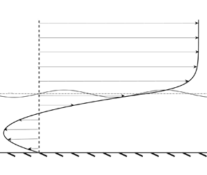
Paquier et al. (Reference Paquier, Moisy and Rabaud2015, Reference Paquier, Moisy and Rabaud2016) in their channel flow experiments observed a flow-reversal profile given by
 \begin{equation} \bar{U}({-}1<\bar{z}<0) = (1 + 4 \bar{z} + 3\bar{z}^2). \end{equation}
One can obtain this velocity profile by solving for the flow in a two-dimensional channel with end walls and with shear stress acting at the free surface. Smith & Davis (Reference Smith and Davis1982) considered a range of velocity profiles varying from linear to quadratic (including flow-reversal profile also) and showed that except for a narrow band of velocity profiles, all the other profiles (particularly, the flow-reversal profile) are susceptible to a viscous long-wave instability. However, Paquier et al. (Reference Paquier, Moisy and Rabaud2015) argues that the flow-reversal velocity profile in the water layer is stable, at least for the cases of high viscosity. In this subsection, we show the presence of an inviscid ‘rippling’ instability of this velocity profile. This occurs due to a critical layer in the water phase similar to Miles instability of the air phase. Following Russell (Reference Russell1994), we simplify the Rayleigh equation to arrive at the spheroidal wave equation using a change of variables. The final form of the non-dimensionalized spheroidal wave equation is
 \begin{equation} \frac{{\rm d}}{{\rm d}\zeta}\left[(1-\zeta^2)\frac{{\rm d}\varPhi}{{\rm d}\zeta}\right] +\left(2-\alpha^2(1-\zeta^2)-\frac{1}{1-\zeta^2}\right)\varPhi = 0, \end{equation}
where
 \begin{equation} \varPhi = \frac{\bar{\phi}}{\sqrt{\bar{U}-\bar{c}}},\quad \alpha = \frac{\bar{k}b}{3},\quad \zeta = \frac{1}{b}(3\bar{z}+2) \quad \text{and}\quad b = \sqrt{1+3\bar{c}}. \end{equation}
The solution of the oblate angular spheroidal wave equation (3.9), using the same notation as Flammer (Reference Flammer1957), is given by
 \begin{equation} \varPhi(\zeta) = a_1 \textrm{S}^{(1)}_{1n}(-{\rm i}\alpha^2,\zeta) + a_2 \text{S}^{(2)}_{1n}(-{\rm i}\alpha^2,\zeta). \end{equation}
Here,  $\text {S}^{(1)}_{1n}$ and $\text {S}^{(2)}_{1n}$ are oblate spheroidal wave functions of first and second kind, respectively, and $a_1$, $a_2$ are integration constants. The spheroidal eigenvalue is $2$ and the value of $n$ can be found from the spheroidal eigenvalue, the coefficient of $-1/(1-\zeta ^2)$ in (3.9) i.e. $1$ and $\alpha ^2$. Therefore, we can write
 \begin{equation}
\bar{\phi}(z) = \sqrt{\bar{U}-\bar{c}}[a_1
\textrm{S}^{(1)}_{1n}(-{\rm
i}\alpha^2,(3\bar{z}+2)/b) + a_2
\text{S}^{(2)}_{1n}(-{\rm
i}\alpha^2,(3\bar{z}+2)/b)].
\end{equation}
\begin{equation}
\bar{\phi}(z) = \sqrt{\bar{U}-\bar{c}}[a_1
\textrm{S}^{(1)}_{1n}(-{\rm
i}\alpha^2,(3\bar{z}+2)/b) + a_2
\text{S}^{(2)}_{1n}(-{\rm
i}\alpha^2,(3\bar{z}+2)/b)].
\end{equation}
An alternative solution to (3.9) can be written in terms of confluent Heun functions and is provided in Appendix A. To the best of our knowledge, this is the first instance in literature where spheroidal wave functions are used in the context of the stability of a shear flow. Substituting (3.12) in the boundary conditions will give the full dispersion relation
 \begin{equation}
\bar{\varXi}_{w}(\bar{c}, \bar{k})(\bar{c}-1)^2 + 4 (\bar{c}-1) -
\mathcal{F}_s(1 + Bo^{{-}1} \bar{k}^2) =0,\end{equation}
\begin{equation}
\bar{\varXi}_{w}(\bar{c}, \bar{k})(\bar{c}-1)^2 + 4 (\bar{c}-1) -
\mathcal{F}_s(1 + Bo^{{-}1} \bar{k}^2) =0,\end{equation}
where
 \begin{align}
\bar{\varXi}_{w}(\bar{c}, \bar{k}) =
\frac{\textrm{S}'^{(1)}_{1n}(-{\rm
i}\alpha^2,2/b)\textrm{S}^{(2)}_{1n}(-{\rm
i}\alpha^2,-1/b)-\textrm{S}'^{(2)}_{1n}(-{\rm
i}\alpha^2,2/b)\textrm{S}^{(1)}_{1n}(-{\rm
i}\alpha^2,-1/b)}{\textrm{S}^{(1)}_{1n}(-{\rm
i}\alpha^2,2/b)\textrm{S}^{(2)}_{1n}(-{\rm
i}\alpha^2,-1/b)-\textrm{S}^{(2)}_{1n}(-{\rm
i}\alpha^2,2/b)\textrm{S}^{(1)}_{1n}(-{\rm
i}\alpha^2,-1/b)}.
\end{align}
\begin{align}
\bar{\varXi}_{w}(\bar{c}, \bar{k}) =
\frac{\textrm{S}'^{(1)}_{1n}(-{\rm
i}\alpha^2,2/b)\textrm{S}^{(2)}_{1n}(-{\rm
i}\alpha^2,-1/b)-\textrm{S}'^{(2)}_{1n}(-{\rm
i}\alpha^2,2/b)\textrm{S}^{(1)}_{1n}(-{\rm
i}\alpha^2,-1/b)}{\textrm{S}^{(1)}_{1n}(-{\rm
i}\alpha^2,2/b)\textrm{S}^{(2)}_{1n}(-{\rm
i}\alpha^2,-1/b)-\textrm{S}^{(2)}_{1n}(-{\rm
i}\alpha^2,2/b)\textrm{S}^{(1)}_{1n}(-{\rm
i}\alpha^2,-1/b)}.
\end{align}
For given values of  $\mathcal {F}_s$, $Bo$ and $\bar {k}$, solving (3.13) will provide the complex eigenvalues $\bar {c}$ and (3.12) provides the eigenfunctions. Initially, we consider the variation of the phase speed ( $\bar {c}_r$) of both prograde and retrograde modes with $\mathcal {F}_s$ at $\bar {k}=0$. Both the modes are stable in this parameter regime and the plot of $\bar {c}_r$ vs $\mathcal {F}_s$ is as shown in figure 4(a). The phase speed of the prograde and retrograde modes start at the maximum and minimum flow velocities, respectively, at $\mathcal {F}_s = 0$. With an increase in $\mathcal {F}_s$, they travel faster but in the opposite direction to each other similar to the case of linear velocity profile.
(a) The non-dimensional phase speed ( $\bar {c}_r$) of prograde and retrograde modes (for the flow-reversal profile) plotted against $\mathcal {F}_s$ (defined in (3.1a,b)). (b) The non-dimensional phase speed ( $\bar {c}_r$) of the stable prograde mode (for the flow-reversal profile) plotted against the non-dimensional wavenumber ( $\bar {k}$) at different $\mathcal {F}_s$.

Figure 4(b) shows the non-dimensional phase speed of the prograde mode (stable in the complete parameter regime) plotted as a function of the wavenumber ( $\bar {k}$) at different $\mathcal {F}_s$. In the limit of $\mathcal {F}_s \rightarrow 0$, the phase speed of the prograde mode coincides with the surface velocity ( $U_s$). At small but finite $\mathcal {F}_s$ ( $= 0.1$ in figure 4a), even though the prograde mode phase speed is different from $U_s$, the variation of its phase speed with wavenumber is not significant. A further increase in $\mathcal {F}_s$ shows that waves with smaller wavelengths travel slower than waves with larger wavelengths. The phase speed and the growth rate of the retrograde mode are plotted as a function of the wavenumber ( $\bar {k}$) in figure 5 for different $\mathcal {F}_s$. The retrograde mode is stable in the long-wave limit $\bar {k} \rightarrow 0$ for $\mathcal {F}_s>0$. Its phase speed deviates from the minimum flow velocity ( $\bar {U}_{min} = -1/3$) in the long-wave limit, coinciding with $\bar {U}_{min}$ only for $\mathcal {F}_s = 0$ (see figure 5a). In contrast to the prograde mode, with an increase in the wavenumber, the phase speed of the retrograde mode increases and crosses $\bar {U}_{min}$ at a particular $\bar {k}$ (for $\mathcal {F}_s>0$). In other words, for $\mathcal {F}_s > 0$, the retrograde mode is stable for $\bar {c}_r \leq -1/3$ and unstable for $\bar {c}_r > -1/3$. The instability occurs because of the presence of a critical layer and a non-zero background velocity curvature if $\bar {c}>-1/3$ as described by Shrira (Reference Shrira1993). In other words, there is a cutoff wavenumber (for $\mathcal {F}_s>0$) below which the growth rate of the retrograde mode is zero (see figure 5b). This cutoff wavenumber shifts to higher values with increasing $\mathcal {F}_s$; simultaneously, the mode becomes less unstable. Similarly, the wavenumber corresponding to the maximum growth rate of the instability increases with increasing $\mathcal {F}_s$.
(a) The non-dimensional phase speed ( $\bar {c}_{r}$), and (b) the non-dimensional growth rate ( $\bar {k}\bar {c}_i$), of the unstable retrograde mode, plotted as a function of the non-dimensional wavenumber ( $\bar {k}$) for different $\mathcal {F}_s$. The four different curves correspond to: ${\mathcal {F}_s}=0$ (black), $0.1$ (blue), $0.5$ (red) and $1$ (green), respectively. The insets in both (a) and (b) show the comparison between the asymptotic approximation for $\mathcal {F}_s=0$ (dashed grey line) from (3.26) and analytical results. The vertical axis of the inset in figure (a) is changed to $\bar {c}_r + 1/3$ for better comparison.

The existence of a long-wave cutoff divides the parameter space into stable and unstable regions. Since the phase speed of the retrograde mode should at least be equal  $\bar {U}_{min}$ for the existence of a critical layer, we substitute $\bar {c} = \bar {U}_{min} = -1/3$ in Rayleigh equation (2.9) to get the following solution:
 \begin{align}
\bar{\phi}(z)= \begin{cases}
\dfrac{2}{3\bar{z}+2}\left[\dfrac{\sinh{\bar{k}(\bar{z}+2/3)}-\bar{k}(\bar{z}+2/3)\cosh{\bar{k}(\bar{z}+2/3)}}{\sinh{(2\bar{k}/3)}-2\bar{k}\cosh{(2\bar{k}/3)}/3}\right],
& \mathrm{for} \ \dfrac{-2}{3}\leq \bar{z}\leq0,\\ 0, &
\mathrm{for} \ -1\leq \bar{z}<\dfrac{-2}{3}, \end{cases}
\end{align}
\begin{align}
\bar{\phi}(z)= \begin{cases}
\dfrac{2}{3\bar{z}+2}\left[\dfrac{\sinh{\bar{k}(\bar{z}+2/3)}-\bar{k}(\bar{z}+2/3)\cosh{\bar{k}(\bar{z}+2/3)}}{\sinh{(2\bar{k}/3)}-2\bar{k}\cosh{(2\bar{k}/3)}/3}\right],
& \mathrm{for} \ \dfrac{-2}{3}\leq \bar{z}\leq0,\\ 0, &
\mathrm{for} \ -1\leq \bar{z}<\dfrac{-2}{3}, \end{cases}
\end{align}and
 \begin{equation} \bar{\varXi}_w ={-}\frac{3}{2}+\frac{2\bar{k}^2}{2\bar{k}\coth{}(2\bar{k}/3)-3}. \end{equation}
The above-simplified form of the eigenfunction appeared due to chosen base state, a quadratic velocity profile. Alternatively, for a more general velocity profile, we can construct a Frobenius’ solution for  $\bar {c} = \bar {U}_{min}$. It is worth highlighting that the Frobenius’ solution at the critical layer, $\bar {c} = \bar {U}_{min}$, contains an algebraic singularity in contrast to the logarithmic singularity of the Tollmien inviscid solutions (Drazin & Reid Reference Drazin and Reid1981) at other locations. A similar algebraic singularity can also be observed for a ‘ $\mathrm {sech}^2(z)$’ (a Bickley jet) velocity profile, at $z = 0$ (i.e. at the critical layer $\bar {c} = \bar {U}_{max}$) (Swaters Reference Swaters1999). Further, the corresponding mode forms a part of the stability boundary too (Maslowe Reference Maslowe1991). The similarity between both scenarios is that the critical layer is at an extremum in the velocity profile; thus, Tollmien inviscid solutions, derived by assuming $\bar {U}'(\bar {z}) \neq 0$, are not applicable in this scenario. However, a Frobenius solution can be derived analogously to Tollmien solutions at the local extremum with Frobenius exponents 2 and $-1$. The two corresponding linearly independent solutions are
 \begin{equation} \left. \begin{aligned} & \bar{\phi}_1(\bar{z})=A_1(\bar{z}-\bar{z}_{cr})^2\left(1+\dfrac{\bar{U}'''_{cr}(\bar{z})}{3\bar{U}''_{cr}(\bar{z})}(\bar{z}-\bar{z}_{cr}) + O(\bar{z}-\bar{z}_{cr})^2\right),\\ & \bar{\phi}_2(\bar{z})=A_2(\bar{z}-\bar{z}_{cr})^{{-}1}\left(1-\dfrac{2\bar{U}'''_{cr}(\bar{z})}{3\bar{U}''_{cr}(\bar{z})}(\bar{z}-\bar{z}_{cr}) + O(\bar{z}-\bar{z}_{cr})^2\right), \end{aligned} \right\} \end{equation}
where,  $A_1$ and $A_2$ are constants of integration and $\bar {z}_{cr}$ is the location of the critical layer. $\phi _2(\bar {z})$ of expressions (3.17) contains a simple pole, i.e. an algebraic singularity if the mode were to be a neutral one. Further analysis can be done to find a uniformly valid solution by considering a small perturbation ( $\delta$) to the phase speed ( $\bar {c} = \bar {U}_{max/min} + \delta$) and constructing solutions in the inner $(|\bar {z}-\bar {z}_{cr}| < \sqrt {\delta })$ and outer $(|\bar {z}-\bar {z}_{cr}| > \sqrt {\delta })$ regions, similar to Swaters (Reference Swaters1999).
For our current problem, we proceed with the analytical solution available. Substituting (3.16) and  $\bar {c}=-1/3$ in the dispersion relation (3.13), we obtain a relation between $\mathcal {F}_s$ and $\bar {k}$ for any particular $Bo^{-1}$ i.e. the stability boundary
 \begin{equation} \mathcal{F}_s ={-}\dfrac{8}{(1+\bar{k}^2Bo^{{-}1})} + \frac{32 \bar{k}^2}{(18 \bar{k}\coth{}(2\bar{k}/3) - 27)(1+\bar{k}^2Bo^{{-}1})}. \end{equation}
Equation (3.18) indicates that the stability boundary curve starts at the origin (in the  $(\mathcal {F}_s,\bar {k})$ plane) and behaves as $\sim 32\bar {k}^2/135$ for $\bar {k}\ll 1$. It must be noted here that expression 3.18 is derived by substituting $\bar {c} = \bar {c}_r=\bar {U}_{min}$ and $\bar {c}_i = 0$ in the Rayleigh equation. However, this does not imply that $\bar {c}_i\neq 0$ if $\bar {c}_r>\bar {U}_{min}$. In other words, the presence of a critical layer and a non-zero background velocity curvature are necessary for instability but not sufficient conditions. Figure 6 shows the stability boundary curve (3.18) for a range of $\bar {k}$ and $\mathcal {F}_s$ over which the growth rates are calculated. The contour, in figure 6, shows the non-dimensional growth rates calculated from the complete dispersion relation. The curve drawn with (3.18) closely traces the stability boundary in the parameter space considered. However, for large $\bar {k}$ and $\mathcal {F}_s$, it is expected that the growth rates will reduce to minimal values and the stability boundary might deviate from the curve given by (3.18). A discussion on the short-wave cutoff and the stability boundary is out of the scope of the current work and is not considered here. Finally, the contour of $\bar {c}_i$ also shows that the most unstable mode exists at small $\mathcal {F}_s$ and moderate $\bar {k}$.
The contour plot of  $\bar {c}_i$ on a grid of the non-dimensional wavenumber $\bar {k}$ as the vertical axis and $\mathcal {F}_s$ as the horizontal axis. The solid, black curve (the stability boundary obtained in (3.18)) demarcates the stable and unstable region in the parameter space.

3.2.2. Long-wave asymptotic calculations
The absence of a cutoff wavenumber for  $\mathcal {F}_s = 0$ can be further understood by a long-wave asymptotic analysis as follows. The leading-order behaviour, of the dispersion relation, in the long-wave limit ( $\bar {k} \to 0$) can be studied using Burns’ integral condition (see Burns Reference Burns1953)
 \begin{equation} \left[\int_{{-}1}^{0} \frac{1}{(\bar{U}(\bar{z})-\bar{c})^2} \, \mathrm{d} \bar{z} \right]-\dfrac{1}{\mathcal{F}_s}=0. \end{equation}
Substituting (3.8) in (3.19) we get the following long-wave dispersion relation for the flow-reversal profile:
 \begin{equation} \left[ \frac{3{\rm i}}{b}\left( \tan^{{-}1}\left(\frac{1}{b^2}\right)+\tan^{{-}1}\left(\frac{2}{b^2}\right)\right) - \frac{9(2-b^2)}{(4-b^2)(1-b^2)} \right] - \dfrac{2 b^2}{\mathcal{F}_s} = 0, \end{equation}
where  $b = \sqrt {1+3\bar {c}}$. Solving the expression (3.20) results in two stable (a prograde and a retrograde) modes. The variation of their phase speed as a function of $\mathcal {F}_s$ is the same as shown in figure 4(a). The behaviour of the growth rate as a function of wavenumber for long waves can also be studied asymptotically. For this, we write an equivalent of the Rayleigh equation (2.9) for the pressure perturbation $\bar {p}(\bar {z})$ as (see Benney & Chow Reference Benney and Chow1986)
 \begin{equation} \left(\frac{\bar{p}'}{(\bar{U}-\bar{c})^2} \right)' - \bar{k}^2 \frac{\bar{p}}{(\bar{U}-\bar{c})^2} = 0, \end{equation}
with the boundary conditions
 \begin{equation} \bar{k}^{2} (1-\bar{c})^{2} \bar{p}(0) - \mathcal{F}_s (1+ Bo^{{-}1} \bar{k}^2) \bar{p}'(0)=0 \ \mathrm{and} \ \bar{p}'({-}1)=0. \end{equation}
We focus on the case of  $\mathcal {F}_s = 0$ and assume $Bo^{-1} = 0$, for simplicity, as an approximation to the air–water scenario. In the limit of $\bar {k}\to 0$, the phase speed is close to $\bar {c}=-1/3$. Therefore, the leading-order equation for the pressure perturbation can be obtained by substituting $\bar {c}=-1/3$ and $\bar {k}=0$ in (3.21). And, to the leading order, the first boundary condition in (3.22) reduces to a Dirichlet condition on the pressure perturbation. Finally, we can write the expression for the pressure perturbation as
 \begin{equation} \bar{p}(\bar{z})= \begin{cases} 1 - \left(\dfrac{3 \bar{z}}{2} +1\right)^{5}, & \mathrm{for} \ 0>\bar{z}>\dfrac{-2}{3},\\ 1, & \mathrm{for} \ \dfrac{-2}{3}>\bar{z}>{-}1. \end{cases} \end{equation}
Now, integrating (3.21) over the domain and applying the boundary conditions (3.22) we get
 \begin{equation} \frac{\bar{p}'(0)}{\left(1-\bar{c}\right)^{2}} = \bar{k}^{2} \int_{{-}1}^{0} \frac{\bar{p}}{(\bar{U}-\bar{c})^2}\, \mathrm{d} \bar{z}. \end{equation}
Assuming  $\bar {p}$ to be close to that in (3.23) and $\bar {c}=-1/3 + \bar {c}_{1}$, such that $\lvert \bar {c}_1 \rvert \ll 1$, we obtain
 \begin{equation} \frac{-135}{32} \sim \bar{k}^2 {\int_{-\infty}^{\infty} \left\{ 3 \left(\bar{z}+ 2/3 \right)^{2} - \bar{c}_{1} \right\}^{{-}2} \, \mathrm{d} \bar{z} } = \bar{k}^{2} \frac{{\rm \pi} }{2 \sqrt{3}} \left( -\bar{c}_{1}\right)^{{-}3/2}, \end{equation}
at the leading order. Thus we get
 \begin{equation} \bar{c}_{1} \sim \left(\frac{16 {\rm \pi}}{135 \sqrt{3}}\right)^{2/3} {\rm e}^{\mathrm{i} {\rm \pi}/3} \bar{k}^{4/3}. \end{equation}
This asymptotic result is in good agreement with the analytical result in the limit of small  $k$ (see the insets of figure 5a,b).
Thus we have demonstrated, using both asymptotic analysis and the complete analytical solution, that a quadratic velocity profile with a free surface is susceptible to instabilities. The mathematical underpinning of the instability is identical to Miles’ mechanism – the presence of a mean vorticity gradient at the critical layer of a surface wave (the backward moving wave in contrast to the forward moving wave for the Miles instability). One can also argue for the physical mechanism of the instability in a manner identical to that proposed by Lighthill (Reference Lighthill1962) for Miles instability – the mean ‘vortex force’ extracting energy from the background flow and transferring it to the surface wave. We will now proceed to the coupled air–water scenario – wherein both the cograde and retrograde surface waves can get destabilized (rippling and Miles instability) and also possibly coexist in some parameter space.
4. Two-phase finite-depth problem: the Miles mode
We will now use the linear stability problem formulated in § 2 to consider the Miles mode of instability arising due to the resonant interaction between the base-state velocity profile in the air and the gravity–capillary waves in the water. In this section, we change the length and velocity scales previously used for non-dimensionalization from  $h$ and $U_s$ (corresponding to the water layer) to $h_a$ and $U_\infty$ (corresponding to the air layer), respectively, to ensure consistency with the previous literature. Here, $h_a$ is the characteristic length scale of the background velocity profile in the air layer, and $U_\infty$ is the free-stream velocity. An over-tilde indicates non-dimensional variables (recall that an over-bar is used in the previous section). Relevant non-dimensional numbers are
 \begin{equation} \mathcal{F}_a = \frac{g h_{a}}{U_{\infty}^{2}},\quad Bo_a = \frac{gh_a^2}{\gamma}, \quad \tilde{U}_s = \frac{U_s}{U_\infty} \quad \mathrm{and}\quad \tilde{h}= \frac{h}{h_{a}}, \end{equation}
where  $\mathcal {F}_a$ and $Bo_a$ are the modified inverse squared Froude number and Bond number, respectively, with the new velocity and length scales. In the following section, the Bond number $Bo_a=1.361\times 10^5$, corresponding to the air–water scenario with a characteristic length scale in the air layer ( $h_a$) of 1 m. The discussion in this section is along the lines of § 7 in Young & Wolfe (Reference Young and Wolfe2014), modified for a finite-depth water domain. We first note that $\epsilon$ defined in (2.11a,b) is a small parameter for the air–water system. The dispersion relation (2.10) can then be rewritten in the following form:
 \begin{equation} \tilde{\mathcal{D}}_{0}(\tilde{c}, \tilde{k}) + \epsilon\, \tilde{\mathcal{D}}_{1}(\tilde{c}, \tilde{k}) =0, \end{equation}
where
 \begin{gather} \tilde{\mathcal{D}}_{0}(\tilde{c}, \tilde{k})= \tilde{\varXi}_{w}(\tilde{c},\tilde{k}) (\tilde{c}-\tilde{U}_{s})^2 + \tilde{S}_{0}\, (\tilde{c}-\tilde{U}_{s}) -\mathcal{F}_a(1+ Bo_a^{{-}1}k^2), \end{gather}
 \begin{gather} \tilde{\mathcal{D}}_{1}(\tilde{c}, \tilde{k})= [\tilde{\varXi}_{a}(\tilde{c},\tilde{k})-\tilde{\varXi}_{w}(\tilde{c},\tilde{k}) ] (\tilde{c}-\tilde{U}_{s})^2 + \tilde{S}_{1}\, (\tilde{c}-\tilde{U}_{s}) +2 \mathcal{F}_a, \end{gather}
with
 \begin{equation} \tilde{S}_{0}=\tilde{U}'(0^{-})\quad \mathrm{and}\quad \tilde{S}_{1}={-}[\tilde{U}'(0^{-})+\tilde{U}'(0^+) ]. \end{equation}
We assume a regular perturbation expansion for  $\tilde {c}(\tilde {k},\epsilon )$ with $\epsilon$ as the small parameter:
 \begin{equation} \tilde{c}(\tilde{k},\epsilon) = \tilde{c}_{0}(\tilde{k}) + \epsilon \tilde{c}_{1}(\tilde{k}) + \cdots. \end{equation}
Expanding  $\tilde {\mathcal {D}}_{0}(\tilde {c},\tilde {k})$ and $\tilde {\mathcal {D}}_{1}(\tilde {c},\tilde {k})$ about $(\tilde {c}_{0},\tilde {k})$ and substituting in (4.2) we get
 \begin{equation} \tilde{\mathcal{D}}_{0}(\tilde{c}_{0}, \tilde{k}) + \epsilon [ \tilde{c}_{1} \partial_{c} \tilde{\mathcal{D}}_{0}(\tilde{c}_{0},\tilde{k}) + \tilde{\mathcal{D}}_{1}(\tilde{c}_{0}, \tilde{k})] + O(\epsilon^2) =0. \end{equation}
 At O( $\epsilon ^0$), we obtain the dispersion relation of gravity–capillary waves modified by a background flow in the water with a free surface at the top
 \begin{equation} \tilde{\mathcal{D}}_{0}(\tilde{c}_{0}, \tilde{k})= 0. \end{equation}
The resonance of the prograde mode from (4.8) with the base-state velocity profile in the air, at a critical layer ( $\tilde {z}=\tilde {z}_{c}>0$) where $\tilde {U}(\tilde {z}_{c})=\tilde {c}_{0}(\tilde {k})$, forms the basis of Miles’ mode. At $O(\epsilon )$, we obtain the correction to the prograde modes’ phase speed due to the background shear flow in the air layer as
 \begin{equation} \tilde{c}_{1} ={-}\frac{\tilde{\mathcal{D}}_{1}(\tilde{c}_{0}, \tilde{k})}{ \partial_{\tilde{c}} \tilde{\mathcal{D}}_{0}(\tilde{c}_{0},\tilde{k})}, \end{equation}
where  $\partial _{\tilde {c}}$ indicates a partial differentiation with $\tilde {c}$. The growth rate of the instability, then, can be written by
 \begin{equation} \tilde{\omega}_{i}(\tilde{k})={-} \epsilon\,\tilde{k} \frac{\mathrm{Im}({\tilde{\mathcal{D}}_{1}(\tilde{c}_{0}, \tilde{k}))}}{\partial_{\tilde{c}} \tilde{\mathcal{D}}_{0}(\tilde{c}_{0},\tilde{k})}. \end{equation}
From (4.4) it is clear that the only components contributing to  $\mathrm {Im}({\tilde {\mathcal {D}}_{1}(\tilde {c}_{0}, \tilde {k}))}$ are $\mathrm {Im}(\tilde {\varXi }_{a}(\tilde {c}_{0},\tilde {k}))$ and $\mathrm {Im}(\tilde {\varXi }_{w}(\tilde {c}_{0},\tilde {k}))$. Multiplying the Rayleigh equation (2.9) by the complex conjugate of the eigenfunction, $\tilde {\phi }^{*}(\tilde {z})$, and then integrating it over the domain, in air and water separately, we find
 \begin{gather} \tilde{\varXi}_{a}(\tilde{c},\tilde{k})=\frac{1}{\left\lvert{\tilde{\phi}_{s}}\right\rvert^2}\int_0^{\infty} \left\lvert\tilde{\phi}'(\tilde{z})\right\rvert^2 + \left( \tilde{k}^2 + \frac{\tilde{U}''(\tilde{z})}{\tilde{U}(\tilde{z})-\tilde{c}(\tilde{k})}\right) \left\lvert\tilde{\phi}(\tilde{z})\right\rvert^2 \, \mathrm{d} \tilde{z} , \end{gather}
 \begin{gather} \tilde{\varXi}_{w}(\tilde{c},\tilde{k})=\frac{1}{\left\lvert{\tilde{\phi}_{s}}\right\rvert^2}\int_{-\tilde{h}}^0 \left\lvert\tilde{\phi}'(\tilde{z})\right\rvert^2 + \left( \tilde{k}^2 + \frac{\tilde{U}''(\tilde{z})}{\tilde{U}(\tilde{z})-\tilde{c}(\tilde{k})}\right) \left\lvert\tilde{\phi}(\tilde{z})\right\rvert^2 \, \mathrm{d} \tilde{z} , \end{gather}
where  $\tilde {\phi }_{s}=\tilde {\phi }(0)$. The imaginary parts of (4.11) and (4.12) are given by
 \begin{equation} \mathrm{Im}(\tilde{\varXi}_{a}(\tilde{c},\tilde{k}))=\frac{\tilde{c}_{i}}{\left\lvert{\tilde{\phi}_{s}}\right\rvert^2}\int_0^{\infty}\frac{\tilde{U}''(z)}{\left\lvert \tilde{U}(z)-\tilde{c}(k)\right\rvert^2} \left\lvert\tilde{\phi}(\tilde{z})\right\rvert^2 \, \mathrm{d} \tilde{z} , \end{equation}
and
 \begin{equation} \mathrm{Im}(\tilde{\varXi}_{w}(\tilde{c},\tilde{k}))=\frac{\tilde{c}_{i}}{\left\lvert{\tilde{\phi}_{s}}\right\rvert^2}\int_{-\tilde{h}}^{0}\frac{\tilde{U}''(\tilde{z})}{\left\lvert \tilde{U}(\tilde{z})-\tilde{c}(\tilde{k})\right\rvert^2} \left\lvert\tilde{\phi}(\tilde{z})\right\rvert^2 \, \mathrm{d} \tilde{z} . \end{equation}
The growth rate,  $\tilde {\omega }_{i}(\tilde {k})$, is proportional to the small parameter $\epsilon$; thus, we take the limit $\tilde {c}_{i}\rightarrow 0$ in (4.13) and (4.14). Since the critical layer is assumed to be in the air ( $\tilde {z}_{c}>0$), (4.14) does not have any singularity in the water domain and goes to zero in the limit of $\tilde {c}_i\rightarrow 0$. However, (4.13) reduces to
 \begin{equation} \mathrm{Im}(\tilde{\varXi}_{a}(\tilde{c},\tilde{k}))={\rm \pi} \frac{\tilde{U}''_{c}}{\left\lvert \tilde{U}'_{c}\right\rvert} \frac{\left\lvert \tilde{\phi}_c\right\rvert ^2}{\left\lvert \tilde{\phi}_s \right\rvert ^2}, \end{equation}
where  $\tilde {U}'_{c}=\tilde {U}'(z_c),\ \tilde {U}''_{c}=\tilde {U}''(z_c)$ and $\tilde {\phi }_{c}=\tilde {\phi }(z_c)$. Substituting these results in (4.10) we obtain (Miles Reference Miles1962)
 \begin{equation} \tilde{\omega}_{i}(\tilde{k})={-}\epsilon\,\tilde{k}\,{\rm \pi} \left(\frac{(\tilde{c}_{0}-\tilde{U}_s)^2}{\partial_{\tilde{c}} \tilde{\mathcal{D}}_{0}(\tilde{c}_{0},\tilde{k})}\right) \frac{\tilde{U}''_{c}}{\left\lvert \tilde{U}'_{c}\right\rvert} \frac{\left\lvert \tilde{\phi}_c\right\rvert ^2}{\left\lvert \tilde{\phi}_s \right\rvert ^2}. \end{equation}
Equation (4.16) makes it evident that the growth rate of the instability is proportional to the negative of the curvature of the velocity profile at the critical layer and only those profiles which are convex at the location of the critical layer (i.e.  $\tilde {U}''_{c}<0$) are unstable. It must be noted here that (4.16) is the same Miles (Reference Miles1957) had for an infinite-depth water layer. This is because the contribution from the water layer to the Miles mode growth rate, given by (4.14), is only through the dispersion relation ( $\tilde {\mathcal {D}}_0(\tilde {c}_0,\tilde {k})$) of the gravity–capillary waves modified by shear flow in the water layer.
For further calculations in this section, we consider an exponential background velocity profile in the air (Young & Wolfe Reference Young and Wolfe2014) given by
 \begin{equation} \tilde{U}(\tilde{z}>0) = 1 - (1 - \tilde{U}_{s}) {\rm e}^{-\tilde{z}}, \end{equation}
where  $\tilde {U}_s$ is the base-state velocity at the air–water interface. Then, the solution to the Rayleigh equation (2.9), for the air layer, can be written in terms of the hypergeometric function $F$ (see Young & Wolfe Reference Young and Wolfe2014) as
 \begin{equation} \tilde{\phi}(\tilde{c},\tilde{k};\tilde{z}>0) = {\rm e}^{-\tilde{k} \tilde{z}} \frac{F(\alpha_a,\beta_a,1+2 \tilde{k};\xi {\rm e}^{-\tilde{z}})}{F(\alpha_a,\beta_a,1+\tilde{k};\xi)}, \end{equation}
where
 \begin{equation} \alpha_a = \tilde{k} - \sqrt{1+ \tilde{k}^2},\quad \beta_a = \tilde{k} + \sqrt{1+ \tilde{k}^2},\quad \xi = \left(\frac{1-\tilde{U}_s}{1-\tilde{c}} \right). \end{equation}
Substituting (4.18) in (4.11), we obtain
 \begin{equation} \tilde{\varXi}_{a}(\tilde{c},\tilde{k}) = \tilde{k} - \frac{\xi}{(1+ 2 \tilde{k})} \frac{F(\alpha_a +1,\beta_a +1,2+2 \tilde{k};\xi)}{F(\alpha_a,\beta_a,1+2 \tilde{k};\xi)}. \end{equation}
From the velocity profile (4.17) and the solution form (4.18), we write
 \begin{gather} \xi_0 = \frac{1-\tilde{U}_{s}}{1-\tilde{c}_{0}(k)}={\rm e}^{\tilde{z}_c}, \quad \dfrac{\tilde{U}''_{c}}{|\tilde{U}'_{c}|} ={-} 1, \end{gather}
 \begin{gather} \tilde{\phi}_{c}(\tilde{c}_{0},\tilde{k}) = \xi_0^{-\tilde{k}} \frac{F(\alpha_a,\beta_a,1+2 \tilde{k};1)}{F(\alpha_a,\beta_a,1+2 \tilde{k};\xi_0)}. \end{gather}
Substituting (4.21a,b) and (4.22) in the growth rate expression (4.16) from Miles’ asymptotic calculation, we can write
 \begin{equation} \tilde{\omega}_{i}(\tilde{k})=\epsilon\,\tilde{k}\,{\rm \pi} \left(\frac{(\tilde{c}_{0}-\tilde{U}_s)^2}{\partial_{\tilde{c}} \tilde{\mathcal{D}}_{0}(\tilde{c}_{0},\tilde{k})}\right)\xi_0^{{-}2\tilde{k}}\left\lvert \frac{F(\alpha_a,\beta_a,1+2 \tilde{k};1)}{F(\alpha_a,\beta_a,1+2 \tilde{k} ;\xi_0)}\right\lvert^2, \end{equation}
by considering that  $\tilde {\phi }_s = 1$, $\tilde {c}_0 < 1$ and $\tilde {U}_s<1$. Using Burns’ long-wave condition (3.19), we can further simplify the expression (4.16) for the long-wave limit. In the limit of $\tilde {k}\rightarrow 0$, (4.22) reduces to
 \begin{equation} \lim_{\tilde{k} \to 0} \tilde{\phi}_{c}(\tilde{c}_{0}(\tilde{k}),\tilde{k}) = \tilde{k} \left(\frac{1- \tilde{c}_{0}(\tilde{k}=0)}{\tilde{U}_{s}-\tilde{c}_{0}(\tilde{k}=0)}\right), \end{equation}
and, the leading-order expression for  $\tilde {\mathcal {D}}_0$, denoted by $\tilde {\mathcal {D}}_0(\tilde {c}_0(0),0)$, is given by the left-hand side term of (3.19); while $\tilde {c}_0(\tilde {k}=0)$ can be obtained from (3.19) for a particular $\mathcal {F}_s$. Substituting (4.21a,b) and (4.24) in (4.16), we obtain
 \begin{equation} \tilde{\omega}_{i}(\tilde{k}\ll1)\sim \epsilon\,\tilde{k}^{3}\,{\rm \pi} \left(\frac{(1-\tilde{c}_{0}(\tilde{k}=0))^2}{\partial_{\tilde{c}} \tilde{\mathcal{D}}_{0}(\tilde{c}_{0}(\tilde{k}=0),0)}\right), \end{equation}
as the leading-order long-wave behaviour of the growth rate of Miles mode for an exponential profile in the air. Expression (4.25) indicates that irrespective of the velocity profile in the water layer, the growth rate varies as  $\sim \tilde {k}^3$ in the long-wave limit. Because this is the long-wave limit, the Miles mode growth rate is lower when compared with the rippling mode growth rate ( $\sim \bar {k}^{7/3}$) given in (3.26).
In the following subsections, we study the effect of the velocity profile in the water layer on Miles mode at finite  $\tilde {k}$. With the exponential profile in the air, we consider a quiescent water layer, a linear velocity profile and the flow-reversal profile in the water. These profiles allow for an analytical solution to the problem.
4.1. Quiescent water layer
Following Miles (Reference Miles1957) we first assume a quiescent water layer albeit of a finite depth. The solution of the Rayleigh equation (2.9), satisfying the boundary condition (2.14) is given by
 \begin{equation} \tilde{\phi}(\tilde{c},\tilde{k};-\tilde{h}<\tilde{z}<0) = \frac{\sinh{\tilde{k}\,(\tilde{z}+\tilde{h})}}{\sinh{\tilde{k}\,\tilde{h}}}, \end{equation}
with
 \begin{equation} \tilde{\varXi}_{w}(\tilde{c},\tilde{k}) = \tilde{k} \coth{\tilde{k} \tilde{h}}, \quad \tilde{S} ={-}\epsilon. \end{equation}
Here, we consider  $\tilde {U}_s = 0$ at the interface for the continuity of velocity profiles.
4.1.1. Solution from the full dispersion relation (2.10)
Substituting the expressions (4.20) and (4.27), we can solve the dispersion relation (2.10) numerically to obtain the complex phase speed of the Miles mode. In figure 7(a,b), we plot the real and imaginary parts of the complex phase speed, at different values of water layer depths ( $\tilde {h}$), as a function of the wavenumber ( $\tilde {k}$). In figure 7(a), the real part of the complex phase speed ( $\tilde {c}_r(\tilde {k})$) is divided by the deep-water gravity–capillary wave speed ( $\tilde {c}_{gc}(\tilde {k})$), given by
 \begin{equation} \tilde{c}_{gc}(\tilde{k}) = \sqrt{\frac{\mathcal{F}_s}{\tilde{k}}(\left(1-2\epsilon\right) +Bo^{{-}1} \tilde{k}^2)}. \end{equation}
This is because the location of the critical layer is defined by the magnitude of the phase speed. The variation of this phase speed, when compared with the deep-water case, can be used as an indication of the growth rate change between finite-depth and deep-water cases. From figure 7(a), assuming a constant  $h_a(=1\,\textrm {m})$, it can be seen that long waves in finite-depth water layers travel slower than gravity–capillary waves in deep water. This indicates that the location of the critical layer in a finite-depth scenario is closer to the interface than in the deep-water case. It has to be recalled here that the growth rate of Miles’ instability is proportional to the magnitude of curvature at the critical layer (see (4.16)). For the exponential velocity profile considered, we see that the curvature is maximum at the interface and decays with height. Therefore, we can conclude that the growth rate of long waves in finite-depth scenario will be more than the growth rate in the deep-water case (see figure 7b). However growth rates for different finite-depth water layer cases can vary non-trivially as is shown in figure 7(b). In addition, we see that with an increase in the wavenumber or the water layer depth, both the phase speeds ( $\tilde {c}_r$ and $\tilde {c}_{gc}$) coincide after a threshold wavelength. This threshold wavelength too is seen to increase with the water layer depth.
For the case of exponential velocity profile in the air and a quiescent water layer: (a) the non-dimensional phase speed ( $\tilde {c}_r/\tilde {c}_{gc}$), where $\tilde {c}_{gc}(\tilde {k})$ is as defined in (4.28), and (b) the non-dimensional growth rate ( $\tilde {k}\tilde {c}_i$) are plotted as a function of the non-dimensional wavenumber ( $\tilde {k}$) for various values of non-dimensional depth ( $\tilde {h}$). The parameters used in this plot are: $U_s= 0\,\mathrm {m}\,\,\mathrm {s}^{-1}$, $h_a= 1\,\mathrm {m}$ and $U_{\infty }=8\,\mathrm {m}\,\,\mathrm {s}^{-1}$.

The growth rate for different  $\tilde {k}$ has a more interesting behaviour when varying $\tilde {h}$ (see figure 7b). At small $\tilde {k}$, smaller-depth water layer cases (small $\tilde {h}$ values) are more unstable as shown, whereas, for intermediate $\tilde {k}$ this behaviour changes non-trivially (for example, $\tilde {h} = 0.1$ has the lowest growth rate). At large $\tilde {k}$, however, all the depths considered have relatively the same growth rate. Furthermore, there exists a long-wave cutoff for larger-depth water layers (for example $\tilde {h} = 10$ and $\infty$ in figure 7b) but not for smaller-depth water layers (see $\tilde {h} = 0.1$ and $1$ in figure 7b). In other words, the water layer depth has an effect of sustaining the Miles instability to longer wavelengths. In summary, for smaller-depth water layers, long waves can be generated on the water surface through Miles instability, whereas a long-wave cutoff exists for larger-depth water layers.
4.1.2. Solution using Miles’ asymptotic calculation
The behaviour of the growth rate can be obtained by writing the Miles asymptotic expression (4.23) for the quiescent water layer as follows. The O( $\epsilon ^0$) expression from the dispersion relation ( $\tilde {\mathcal {D}}_0$) and the corresponding phase speed of the gravity–capillary waves ( $\tilde {c}_0$), can be obtained by substituting the results from (4.27) in (4.3) and (4.8) to get
 \begin{equation} \tilde{\mathcal{D}}_{0}(\tilde{c}, \tilde{k})= \tilde{k}\, \coth{k h}\, \tilde{c}^2 - \mathcal{F}_a(1+Bo_a^{{-}1} \tilde{k}^2),\quad\textrm{and}\quad \tilde{c}_{0}( \tilde{k})=\sqrt{\frac{\mathcal{F}_a}{\tilde{k}}(\!1 + Bo_a^{{-}1} \tilde{k}^2\!)\tanh{\tilde{k} \tilde{h}}}, \end{equation}
respectively. From the expressions (4.29a,b) and (4.21a,b), we can write
 \begin{equation} \partial_{\tilde{c}}\tilde{\mathcal{D}}_0(\tilde{c}_0,\tilde{k}) = 2\tilde{k}\tilde{c}_0\coth \tilde{k}\tilde{h}\quad \text{and}\quad \xi_0 = \left(1-\widetilde{c_0}\right)^{{-}1}. \end{equation}
By substituting the first expression of (4.30a,b) in (4.23), we obtain
 \begin{equation} \sigma = \frac{1}{\epsilon}\tilde{\omega}_{i}(\tilde{k}) = \frac{\rm \pi}{2}\,\tilde{c}_0\,\xi_0^{{-}2 \tilde{k}}\tanh{\tilde{k}\tilde{h}}\,\left\lvert \frac{F(\alpha_a,\beta_a,1+2 \tilde{k};1)}{F(\alpha_a,\beta_a,1+2 \tilde{k};\xi_0)} \right\rvert^2, \end{equation}
where  $\tilde {c}_0(\tilde {k})$ is given by (4.29a,b). We have verified these results from the asymptotic analysis with the results obtained in § 4.1.1 and they are in agreement with each other, validating the Miles asymptotic solution. An advantage of the asymptotic analysis is that we now have an analytical expression for the growth rate of the instability (4.31).
4.1.3. Stability boundary
From (4.31), we find that a long-wave cutoff exists when  $(1-\tilde {c}_0) = 0$, i.e. for
 \begin{equation} \frac{\mathcal{F}_a}{\tilde{k}}(1 + Bo_a^{{-}1}\tilde{k}^2 ) \tanh{\tilde{k} \tilde{h}}=1. \end{equation}
In other words, if  $\tilde {c}_0 > 1$, the gravity–capillary wave phase speed ( $c_0$) will be greater than the maximum background flow velocity in the air ( $U_\infty$). This implies that the unstable Miles mode becomes a stable prograde mode for the air–water system and (4.31) for the growth rate, which assumes that $c_0\leq U_\infty$, is no longer applicable. For a particular $Bo_a$, the curve given by (4.32) forms a part of the stability boundary that demarcates stable and unstable regions in the $\tilde {k}\tilde {h}$ and $\mathcal {F}_a\tilde {h}$ plane (as can be seen by the black curve in figure 8). In the limit of $\tilde {k}\tilde {h} \to 0$, (4.32) can be rewritten as $\mathcal {F}_a\tilde {h} = 1+(1-3Bo_a^{-1}\tilde {h}^{-2})\tilde {k}^2\tilde {h}^{2}/3$ i.e. for $\tilde {k}\tilde {h} = 0$ the stability boundary starts at $\mathcal {F}_a\tilde {h} = 1$, irrespective of $Bo_a$, and the region given by $\mathcal {F}_a\tilde {h}<1$ is unstable. For the air–water system, $Bo_a^{-1}$ is a small number. Therefore to the leading order in $Bo_a^{-1}$, (4.32) can be rewritten as
 \begin{equation} \frac{\tanh{\tilde{k} \tilde{h}}}{\tilde{k} \tilde{h}}=\frac{1}{\mathcal{F}_a \tilde{h}}. \end{equation}
For long waves, (4.33) implies that  $\mathcal {F}_a\tilde {h} \sim \tilde {k}^2\tilde {h}^2$. That is, the long-wave stability boundary behaves in the same way as $Bo_a^{-1} \to 0$. For short waves, however, (4.32) exhibits a singular behaviour for vanishing $Bo_a^{-1}$. Assuming $Bo_a^{-1} \neq 0$, (4.32) shows that $\mathcal {F}_a \tilde {h} \to 0$ as $\tilde {k}\tilde {h} \to \infty$. Because the curve provided by (4.32) traces the loci of the points where $\tilde {c}_0 = 1$, the region enclosed by this curve and the line $\mathcal {F}_a\tilde {h} = 0$ provide an upper limit of the unstable region. Furthermore, this implies that the stability boundary is concave (leftwards) and will have a maximum $\mathcal {F}_a\tilde {h}$. In figure 8, both dashed and continuous black curves show the long-wave stability boundary (4.32) for two different $\tilde {h}$ ( $= 0.1$ and $1$, respectively) at a Bond number corresponding to the air–water parameters. Here, the concavity is not apparent because only a limited range of wavenumbers are shown. But it is clearly observable for the case of linear velocity profile in the water layer, which we will describe in the next subsection.
Stability boundary curves for the exponential velocity profile in the air and a linear velocity profile in water, obtained by solving (4.43). Here, the non-dimensional wavenumber  $\tilde {k}\tilde {h}$ is plotted against $\mathcal {F}_a \tilde {h}$ (as defined in (4.1a–d)). The black curve ( $\tilde {U} = 0$) corresponds to the case of exponential velocity profile in the air and a quiescent water layer (see (4.32)). The dashed lines are for $\tilde {h} = 1$ and the continuous lines are for $\tilde {h} = 0.1$.

In summary, an infinite-depth problem ( $\tilde {h} \rightarrow \infty$) with a quiescent water always has a long-wave cutoff without any constraint on the value of $\mathcal {F}_a$; on the other hand, for a finite-depth problem, existence of a long-wave cutoff depends on the parameters ( $\mathcal {F}_a, Bo_a^{-1}$) considered. Physically, in dimensional terms, it can be explained using the gravity–capillary wave speed ( $c_{0}(k)$) in the limit $k\rightarrow 0$. For an infinite-depth problem, $c_{0}(k) = \sqrt {{g}/{k} + \gamma k}$. It is unbounded as $k\rightarrow 0$. On the other hand, for a finite-depth problem with a quiescent water, $c_0(k) = \sqrt {({g}/{k} + \gamma k) \tanh (k h)}$. For $k\rightarrow 0$, the limit is finite and is equal to $\sqrt {gh}$. For the infinite-depth problem, below a particular $k$,
$k$,  $c_{0}(k)$ will be higher than $U_{\infty }$. In such a case, no critical layer would exist below that wavenumber, resulting in a long-wave cutoff. But for the finite-depth, since the $c_{0}(k)$ is bounded by $\sqrt {gh}$, a cutoff would exist only if $\sqrt {gh}>U_{\infty }$ i.e. $1 < \mathcal {F}_a\tilde {h}$.
4.1.4. Long-wave behaviour of growth rate ( $\sigma$)

For the case of  $\mathcal {F}_a\tilde {h} < 1$, in the limit of $\tilde {k}\ll 1$, the leading-order expression for the growth rate can be obtained by an expansion of (4.31) for low- $\tilde {k}$, and is given by
 \begin{equation} \sigma = \frac{\rm \pi}{2} {\tilde{k}}^3 \sqrt{\frac{\tilde{h}}{\mathcal{F}_a}} \left( 1- \sqrt{\mathcal{F}_a \tilde{h}}\right)^2. \end{equation}
Expression (4.34) can also be derived from Burns’ long-wave expression (4.25). The growth rate varies as  $\sim \tilde {k}^3$ for small $\tilde {k}$, as is shown in the expression (4.25). For a given $\mathcal {F}_a$ and $\tilde {k}$, $\sigma$ has a local maximum at $\tilde {h}_{max} = 1/(9\mathcal {F}_a)$. In other words, there exists a $\tilde {h}$ ( $=\tilde {h}_{max}$) at which long waves are more unstable than for other $\tilde {h}$. Finally, for the parameters shown in figure 7(b) (i.e. $\mathcal {F}_a = 0.15$), we see from (4.34) that the long-wave growth rate for $\tilde {h} = 0.1$ is smaller than for $\tilde {h} = 1$, which we expect will be true for smaller values of $\tilde {k}$ than what is presented in figure 7(b), because of the slope of the curves.
4.2. Linear velocity profile in the water layer
Recently, Kharif & Abid (Reference Kharif and Abid2020) and Abid & Kharif (Reference Abid and Kharif2021) considered a linear velocity profile in the water layer and a logarithmic velocity profile in the air layer in their study of the role of water layer vorticity and finite-depth on the Miles instability. For a particular wave age, they showed that the wave growth rate is inversely (directly) proportional to the water layer vorticity (depth) and provided expressions for the same. Additionally, here we derive the expressions for the long-wave behaviour of the growth rate, for the stability boundary and discuss different limits of the same. We follow § 4.1 and consider an exponential velocity profile in the air layer. The expressions for  $\tilde {\phi }$ and $\tilde {\varXi }_a$ are as given in the (4.18) and (4.20), respectively. In the water layer, we consider a linear velocity profile studied in § 3.1:
 \begin{equation} \tilde{U}(-\tilde{h}<\tilde{z}<0) = \tilde{U}_{s}\left(1+\dfrac{\tilde{z}}{\tilde{h}}\right). \end{equation}
The expressions for  $\tilde {\phi }$ and $\tilde {\varXi }_{w}$ are the same as in (4.26) and (4.27), respectively. However, the expression for $\tilde {S}$ changes to
 \begin{equation} \tilde{S} = \frac{\tilde{U}_s}{\tilde{h}} -\epsilon \left(\frac{\tilde{U}_{s}}{\tilde{h}} + (1-\tilde{U}_{s})\right). \end{equation}
The existence of a velocity profile, in the water layer, includes another parameter (surface velocity,  $\tilde {U}_s$) in the list of parameters ( $\tilde {k}$, $\tilde {h}$, $\mathcal {F}_a$, $Bo_a^{-1}$) that affect Miles instability. It has to be noted here that the limit of $\tilde {U}_s\to 0$ can be treated as the quiescent water layer problem.
4.2.1. Solution using the full dispersion relation
Using (4.36) and the expression for  $\tilde {\varXi }_w$ in (4.26), the full dispersion relation (2.10) is solved for different $\tilde {U}_{s}$ at $\tilde {h}=0.1$, as shown in figure 9, and for different $\tilde {h}$ at $\tilde {U}_{s}= 3 \tilde {c}_{min}$, as shown in figure 10, respectively. The quantity $\tilde {c}_{min}$, referred to above and used in figures 9 and 10, is the minimum value of $\tilde {c}_{gc}(\tilde {k})$ and is given by $\tilde {c}_{min}=[4\, (1-2\epsilon )\mathcal {F}_a^2Bo_a^{-1}]^{1/4}$.
For the exponential profile in the air and the linear velocity profile in the water: (a) the non-dimensional phase speed ( $\tilde {c}_r/\tilde {c}_{gc}$), and (b) the growth rate ( $\tilde {k}\tilde {c}_i$) plotted as a function of non-dimensional wavenumber ( $\tilde {k}$) at different surface velocities ( $\tilde {U}_s$). The inset in (b) shows the variation of the growth rate over a larger range of $\tilde {k}$. The parameters used in this plot are: $h= 0.1\,\mathrm {m}$, $h_a=1\,\mathrm {m}$ and $U_{\infty }=8\,\mathrm {m}\,\mathrm {s}^{-1}$.

For the exponential profile in the air and the linear velocity profile in the water: (a) the non-dimensional phase speed ( $\tilde {c}_r/\tilde {c}_{gc}$), and (b) the non-dimensional growth rate ( $\tilde {k}\tilde {c}_i$) plotted as a function of non-dimensional wavenumber ( $\tilde {k}$) at different non-dimensional depth's ( $\tilde {h}$). The parameters used in the plot are: $\tilde {U}_s= 3\tilde {c}_{min}$, $h_a= 1\,\mathrm {m}$ and $U_{\infty }=8\,\mathrm {m}\,\mathrm {s}^{-1}$.

Figure 9(a) shows that long waves travel slower than the gravity–capillary wave speed ( $\tilde {c}_{gc}$) irrespective of the surface velocity ( $\tilde {U}_s$) and have relatively the same phase speeds at various surface velocities. This corresponds to higher Miles mode growth rates. However, short waves travel faster than $\tilde {c}_{gc}$ (except for $\tilde {U}_s = 0$, which coincides with the quiescent water layer result) indicating a reversal in the growth rate behaviour. Further, it can also be observed from figure 9(a) that the phase speeds of short waves increase proportional to the surface velocity, $\tilde {U}_{s}$. Figure 9(b) shows the variation of growth rate with the wavenumber at different values of $\tilde {U}_s$. For small $\tilde {k}$ (in the parameter regime shown), increasing the $\tilde {U}_s$ makes the flow more unstable (for example, at $\tilde {k}=10^{-1}$, $\tilde {U}_s=3 \tilde {c}_{min}$ has the largest growth rate); on the other hand, for an intermediate $\tilde {k}$, the growth rate order is reversed. In the short-wave limit, $\tilde {k}\gg 1$, the growth rate is relatively the same for different surface speeds (refer to the inset in figure 9). Figure 9 does not show any long-wave cutoff, because of the $\tilde {h}$ chosen.
Figure 10(a) shows that, similar to the case of the quiescent water layer, long waves, for a given  $\tilde {U}_s$ ( $= 3\tilde {c}_{min}$), have slower phase speeds in the smaller-depth water layers than in the larger-depth water layers (compare $\tilde {h} = 0.1$ and $\tilde {h} = 10$ in figure 10a). At large $\tilde {k}$, the phase speeds ( $\tilde {c}_r$) of different $\tilde {h}$ are relatively the same, although higher than $\tilde {c}_{gc}$. It has to be noted here that the case of $\tilde {h} = \infty$ is avoided here because the linear background velocity profile results in either unphysically large surface velocities or negligible shear rates in an unbounded domain. The variation of the growth rate as a function of the wavenumber is as shown in figure 10(b) and is similar to the quiescent water layer case in figure 7(b). The relative order of growth rates for various water layer depths is again different for small and intermediate values of $\tilde {k}$. For instance, $\tilde {h}=0.1$ has the highest growth rate among the water layer depths considered at $\tilde {k}=10^{-1}$; on the other hand, it is least unstable for $\tilde {k}=1$. The growth rates are again almost the same for all the cases for large values of $\tilde {k}$. The long-wave cutoff exists for larger-depth water layers (for example, $\tilde {h} = 10$) and the maximum growth rate occurs at moderate wavenumbers irrespective of the water layer depth.
4.2.2. Solution using Miles’ asymptotic calculation
The  $O(\epsilon ^0)$ expression from the dispersion $\tilde {\mathcal {D}}_{0}(\tilde {c},\tilde {k})$ can be written, by substituting both $\tilde {\varXi }_w$ from the (4.26) and $S$ from expression (4.36) in (4.3), as
 \begin{equation} \tilde{\mathcal{D}}_{0}(\tilde{c}, \tilde{k})= \tilde{k} \coth{\tilde{k} \tilde{h}} (\tilde{c}-\tilde{U}_{s})^2 + \frac{\tilde{U}_{s}}{\tilde{h}}\, (\tilde{c}-\tilde{U}_{s}) - \mathcal{F}_a(1+ Bo_a^{{-}1} \tilde{k}^2). \end{equation}
The phase speed at O( $\epsilon ^{0}$) is the same as the phase speed of the modified prograde gravity–capillary wave given in (3.6) but with air layer non-dimensionalization. Therefore
 \begin{equation} \partial_{\tilde{c}}\tilde{\mathcal{D}}_0(\tilde{c}_0,\tilde{k}) = 2 \tilde{k} (\tilde{c}_0 - \tilde{U}_s) \coth{\tilde{k} \tilde{h}} + \dfrac{\tilde{U}_s}{\tilde{h}}. \end{equation}
The non-dimensional growth rate is given by
 \begin{equation}
\sigma(\tilde{h},\tilde{U}_s,Fr_a,Bo_a,\tilde{k}) =
\dfrac{{\rm \pi} {v_{0}}^2\xi_0^{{-}2 \tilde{k}}\left\lvert
\dfrac{F(\alpha_a,\beta_a,1+2
\tilde{k};1)}{F(\alpha_a,\beta_a,1+2\tilde{k};\xi_0)}
\right\rvert^2}{\left[\left(\dfrac{\tilde{U}_s}{\tilde{k}\tilde{h}}
\right)^{2}+ 4 \dfrac{\mathcal{F}_a}{\tilde{k}}(1 + Bo_a^{{-}1}\tilde{k}^2) \coth{\tilde{k}
\tilde{h}}\right]^{1/2}} ,
\end{equation}
\begin{equation}
\sigma(\tilde{h},\tilde{U}_s,Fr_a,Bo_a,\tilde{k}) =
\dfrac{{\rm \pi} {v_{0}}^2\xi_0^{{-}2 \tilde{k}}\left\lvert
\dfrac{F(\alpha_a,\beta_a,1+2
\tilde{k};1)}{F(\alpha_a,\beta_a,1+2\tilde{k};\xi_0)}
\right\rvert^2}{\left[\left(\dfrac{\tilde{U}_s}{\tilde{k}\tilde{h}}
\right)^{2}+ 4 \dfrac{\mathcal{F}_a}{\tilde{k}}(1 + Bo_a^{{-}1}\tilde{k}^2) \coth{\tilde{k}
\tilde{h}}\right]^{1/2}} ,
\end{equation}
where
 \begin{gather} \xi_0 = \left(1- \dfrac{v_{0}}{1-\tilde{U}_s}\right)^{{-}1} \quad \text{and} \end{gather}
 \begin{gather} v_{0}=\frac{1}{2} \left[ -\left(\frac{\bar{U}_s}{\tilde{k}\tilde{h}} \tanh{\tilde{k} \tilde{h}} \right) + \left \{ \left(\frac{\bar{U}_s}{\tilde{k}\tilde{h}} \tanh{\tilde{k} \tilde{h}} \right)^{2} + 4 \dfrac{\mathcal{F}_a}{\tilde{k}}(1 + Bo_a^{{-}1}\tilde{k}^2 ) \tanh{\tilde{k} \tilde{h}} \right \}^{1/2} \right], \end{gather}
and all the other parameters are the same as in (4.1a–d). The expression (4.39) is in good agreement with the growth rate obtained from the full dispersion relation. Further, it can be easily seen that for  $\tilde {U}_s = 0$, the growth rate expression (4.39) becomes expression (4.31) for the quiescent water layer.
4.2.3. Stability boundary
The long-wave stability boundary, for this scenario, can be obtained from the growth rate expression (4.39) where, a cutoff exists for  $\xi _0^{-1} = 0$. In other words, for
 \begin{equation} v_{0}= 1-\tilde{U}_s. \end{equation}
Simplifying the above expression, we can write
 \begin{equation}
\frac{\tanh{\tilde{k} \tilde{h}}}{\tilde{k} \tilde{h}}=
\frac{( 1-\tilde{U}_s)^{2}}{[\mathcal{F}_a\tilde{h}(1 + Bo_a^{{-}1} {\tilde{k}}^2) - \tilde{U}_s (1-\tilde{U}_s)]}. \end{equation}
\begin{equation}
\frac{\tanh{\tilde{k} \tilde{h}}}{\tilde{k} \tilde{h}}=
\frac{( 1-\tilde{U}_s)^{2}}{[\mathcal{F}_a\tilde{h}(1 + Bo_a^{{-}1} {\tilde{k}}^2) - \tilde{U}_s (1-\tilde{U}_s)]}. \end{equation}
In the limit of  $\tilde {k}\tilde {h} \to 0$, we can write $\mathcal {F}_a\tilde {h} = (1-\tilde {U}_s)+((1-\tilde {U}_s)^2/3-Bo_a^{-1}(1-\tilde {U}_s)/\tilde {h})\tilde {k}^2\tilde {h}^2$; therefore for $\tilde {k}\tilde {h}= 0$, the stability boundary starts at $\mathcal {F}_a\tilde {h} = (1 - \tilde {U}_s)$. Similarly, in the limit of $\tilde {k}\tilde {h} \to \infty$, we have $\mathcal {F}_a\tilde {h} \to 0$. This behaviour for large $\tilde {k}\tilde {h}$ is as already discussed in the previous subsection § 4.1.3 for the quiescent water layer. In other words, for $Bo_a^{-1} \neq 0$, the region enclosed by the curve (4.43) is bounded, resulting in an upper boundary for the unstable region.
Figure 8 shows the behaviour of the stability boundary in the  $\mathcal {F}_a \tilde {h}$ and $\tilde {k}\tilde {h}$ plane for different $\tilde {U}_s$ and $\tilde {h}$. The continuous and dashed lines are for $\tilde {h} = 0.1$ and $1$, respectively. Both dashed and continuous curves start at the same $\mathcal {F}_a\tilde {h}$ for $\tilde {k}\tilde {h} = 0$ and deviate from each other as $\mathcal {F}_a\tilde {h}$ is increased. For $\tilde {h} = 1$, the dashed curves vary linearly with $\tilde {k}\tilde {h}$ at least up to $\tilde {k}\tilde {h} = 20$. For $\tilde {h} = 0.1$ (continuous curves), the curvature is clearly observable even for $\tilde {k}\tilde {h} < 20$ and large deviations from the linear behaviour occur at higher values of $\tilde {U}_s$ (see $\tilde {U}_s = 0.25$ in figure 8, for example). As $\tilde {U}_s \to 0$, the stability boundary corresponding to the quiescent water layer can be recovered.
4.2.4. Long-wave behaviour of growth rate ($\sigma$)

Similar to § 4.1.4 a long-wave expansion for  $\sigma$ can be carried out in this case too. The leading-order term in the $\tilde {k}\ll 1$ expansion is given by
 \begin{equation} \sigma = \frac{\rm \pi}{4} {\tilde{k}}^3 \tilde{h}\frac{\left({-}2 +\tilde{U}_s + \sqrt{\tilde{U}_s^2+ 4 \mathcal{F}_a \tilde{h}} \right)^2}{\sqrt{\tilde{U}_s^2+ 4 \mathcal{F}_a \tilde{h}}}. \end{equation}
This expression can also be derived from the Miles asymptotic expression (4.25) and in the limit of  $\tilde {U}_s = 0$, will be the same as (4.34). For a given $\tilde {k}$, $\mathcal {F}_a$ and $\tilde {U}_s$ the variation of growth rate with $\tilde {h}$ is similar to the case of quiescent water layer i.e. there is a maximum $\tilde {h}$ ( $=\tilde {h}_{max}$) at which the long-wave growth rate attains a maximum. For a given $\tilde {k}$, $\mathcal {F}_a$ and $\tilde {h}$, growth rate decreases with an increase in $\tilde {U}_s$ until the limit at $\tilde {U}_s = 1 - \mathcal {F}_a\tilde {h}$. For the parameters used in figure 9(b) ( $\mathcal {F} = 0.15, \tilde {h} = 0.1$), the growth rate from $\tilde {U}_s = 0$ is verified to be more than the growth rate from $\tilde {U}_s = 3\tilde {c}_{min}$; however, this happens at a smaller $k$ than which is shown in figure 9. Similarly, for the parameters used in figure 10, the growth rate of $\tilde {h} = 1$ is more than the growth rate from $\tilde {h} = 0.1$.
4.3. The flow-reversal profile in the water
The flow-reversal profile given in Paquier et al. (Reference Paquier, Moisy and Rabaud2015) is considered in the water layer similar to § 3.2:
 \begin{equation} \tilde{U}(-\tilde{h}<\tilde{z}<0) = \tilde{U}_{s}\left\{1 + 4 \frac{\tilde{z}}{\tilde{h}} + 3\left( \frac{\tilde{z}}{\tilde{h}}\right)^2 \right\}. \end{equation}
The expressions for  $\tilde {\phi }$ and $\tilde {\varXi }_w$ are as given in (3.12) and (3.13), respectively. And, we have
 \begin{equation} \tilde{S} = \frac{4\tilde{U}_{s}}{\tilde{h}} -\epsilon \left(\frac{4\tilde{U}_{s}}{\tilde{h}} + (1-\tilde{U}_{s})\right). \end{equation}
As can be seen in § 3.2, the retrograde mode of the flow-reversal profile becomes unstable for a range of parameters. Since, by definition, the phase speed of the prograde mode is always higher than the maximum water current speed (or the surface velocity  $U_s$ in the present case), it is stable in the absence of the air. However, with air being present, the prograde mode can become the Miles mode of instability provided the phase speed of the prograde mode is less than the free-stream velocity.
4.3.1. Solution to the full dispersion relation
Substituting the expressions (3.12), (3.13), (4.20) and (4.46) in (2.10) and suitably non-dimensionalizing (see § 4.1.2), we get the dispersion relation
 \begin{align}
&[\epsilon \tilde{\varXi}_{a}(\tilde{c}, \tilde{k})+(1-\epsilon)
\tilde{\varXi}_{w}(\tilde{c}, \tilde{k}) ] (\tilde{c}-\tilde{U}_s)^2\nonumber\\
&\quad + \bar{S} (\tilde{c}-\tilde{U}_s) - \mathcal{F}_a (1- 2 \epsilon+Bo_a^{{-}1}\tilde{k}^2) =0. \end{align}
\begin{align}
&[\epsilon \tilde{\varXi}_{a}(\tilde{c}, \tilde{k})+(1-\epsilon)
\tilde{\varXi}_{w}(\tilde{c}, \tilde{k}) ] (\tilde{c}-\tilde{U}_s)^2\nonumber\\
&\quad + \bar{S} (\tilde{c}-\tilde{U}_s) - \mathcal{F}_a (1- 2 \epsilon+Bo_a^{{-}1}\tilde{k}^2) =0. \end{align}
We solve (4.51) numerically, using a root-finding routine in Mathematica, to get the respective eigenvalues of rippling and Miles modes. In figure 11(a), we show the variation of the non-dimensional phase speed ( $\tilde {c}_r/\tilde {c}_{gc}$) of Miles’ mode as a function of the wavenumber for various $\tilde {h}$. The similarity between the figures 10(a) and 11(a) indicates the absence of any change in the fundamental behaviour of phase speed vs $\tilde {k}$ with a change in background flow in the water layer. The only difference, however, is that the phase speed of short waves in smaller-depth water layers of figure 11(a) is clearly different from larger-depth water layers, unlike the case of figure 10(a). The variation of non-dimensional growth rate ( $\tilde {k}\tilde {c}_i$) as a function of non-dimensional wavenumber ( $\tilde {k}$), for different $\tilde {h}$, is given in figure 11(b). It is shown that the growth rate has a maxima at moderate $\tilde {k}$ and rapidly decays for large $\tilde {k}$. The absence of long-wave cutoff for smaller-depth water layers is also observed in this case of flow-reversal profile in the water layer. Similar to figure 11(a), a difference between the growth rates of smaller and larger-depth water layers exists for figure 11(b).
For the exponential velocity profile in the air and the flow-reversal profile in the water: (a) the non-dimensional phase speed ( $\tilde {c}_r/\tilde {c}_{gc}$), and (b) the non-dimensional growth rate ( $\tilde {k}\tilde {c}_i$), plotted as a function of non-dimensional wavenumber ( $\tilde {k}$) at different non-dimensional depth's ( $\tilde {h}$). The parameters used in the plot are: $\tilde {U}_s= 3\tilde {c}_{min}$, $h_a= 1\,\mathrm {m}$ and $U_{\infty }=8\,\mathrm {m}\,\mathrm {s}^{-1}$.

4.3.2. Stability boundary (for both the rippling and Miles instabilities)
As shown in §§ 4.1 and 4.1.4, a cutoff for Miles instability occurs when  $\tilde {c} = 1$, i.e. when the phase speed of the Miles mode matches with the free-stream velocity $U_\infty$. The eigenfunction for the air layer, then, can be reduced to $\tilde {\phi } = \exp (-\tilde {z}\sqrt {\tilde {k}^2+1})$, therefore, $\tilde {\varXi }_a = \sqrt {\tilde {k}^2+1}$. Substituting $\tilde {\varXi }_a$ in (4.51), we obtain the stability boundary
 \begin{align}
\mathcal{F}_a = \dfrac{1}{(1- 2 \epsilon + Bo^{{-}1}_a\tilde{k}^2)
}[[ \epsilon \, \sqrt{\tilde{k}^2+1}+(1-\epsilon ) \,
\tilde{\varXi}_{w} ] (1-\tilde{U}_s)^2 +
\tilde{S} \, (1-\tilde{U}_s)].
\end{align}
\begin{align}
\mathcal{F}_a = \dfrac{1}{(1- 2 \epsilon + Bo^{{-}1}_a\tilde{k}^2)
}[[ \epsilon \, \sqrt{\tilde{k}^2+1}+(1-\epsilon ) \,
\tilde{\varXi}_{w} ] (1-\tilde{U}_s)^2 +
\tilde{S} \, (1-\tilde{U}_s)].
\end{align}
Here, it has to be noted that,  $\tilde {\varXi }_w$ is given by (3.14) with $\tilde {c} = 1$. For the rippling instability, substituting $\tilde {c}=-\tilde {U}_s/3$ will result in
 \begin{equation} \tilde{\varXi}_w = \dfrac{-3}{2\tilde{h}}+\dfrac{2\tilde{k}^2\tilde{h}}{2\tilde{k}\tilde{h}\coth(2\tilde{k}\tilde{h}/3)-3}, \end{equation}
and
 \begin{equation} \mathcal{F}_a = \dfrac{1}{(1- 2 \epsilon + Bo^{{-}1}_a\tilde{k}^2) }\left[\frac{16}{9}\tilde{U}_s^2\left[ \epsilon \tilde{\varXi}_{a}+\left(1-\epsilon \right) \tilde{\varXi}_{w} \right] -\frac{4}{3}\bar{S}\,\tilde{U}_s \right], \end{equation}
gives the stability boundary. Here,  $\tilde {\varXi }_a$ is given by (4.20) with $\tilde {c} = -\tilde {U}_s/3$.
In figure 12, the stability regions of both the rippling and Miles modes are presented in vertically aligned  $(\mathcal {F}_a$, $\tilde {k})$ planes at specific values of $\tilde {U}_s$ and $\tilde {h}$. The contour plot in the first two planes of each figure indicates the log of the non-dimensional growth rate ( $\tilde {c}_i$) ranging from minimum (yellow) to maximum (blue) values. Growth rates less than $10^{-10}$ are neglected for numerical convenience. Therefore, the edge of the contour should not be confused with the stability boundary. The expressions given by (4.48) and (4.50) provide the curves at which $\tilde {c} = 1$ and $-\tilde {U}_s/3$, respectively. That is, at least in the initial range of $(\mathcal {F}_a,\tilde {k})$ shown in figure 12(a–d), these curves form a part of the stability boundaries of the Miles and rippling instabilities, respectively. They are shown by continuous and dashed curves for Miles and rippling instability, respectively. In the third plane of each figure, we show different regions of instability demarcated as: the stable region (S), the region where the Miles instability (M) growth rate is maximum, and the region where the rippling instability (R) is maximum. It has to be reiterated that to draw the boundaries of the unstable regions, a cutoff growth rate (of $10^{-10}$) is assumed.
The rippling and Miles instability growth rate contours plotted in the plane of non-dimensional wavenumber ( $\tilde {k}$) and inverse square Froude number ( $\mathcal {F}_a$) stacked vertically for better visibility. The base-state horizontal velocity profile in the air layer is an exponential profile, and in the water layer, it is a flow-reversal profile. In each figure, the bottom plane demarcates different stability regions: (S) – stable region, (M) – the region where the Miles instability growth rate is more than the rippling instability growth rate and (R) – the region where the rippling instability growth rate is more than the Miles instability growth rate. The continuous (in the mid-plane) and dashed (in the upper plane) lines are the stability boundary curves obtained from (4.48) and (4.50), respectively. The parameters considered are: (a) $\tilde {U}_s = 1/2$ and $\tilde {h} = 1$, (b) $\tilde {U}_s = 1/8$ and $\tilde {h} = 1$,(c) $\tilde {U}_s = 1/8$ and $\tilde {h} = 10$ and (d) $\tilde {U}_s = 1/8$ and $\tilde {h} = 0.1$.

Figure 12(a,c) show the stability regions at constant  $\tilde {h}$ ( $=1$) but for different $\tilde {U}_s$. It can be seen that with an increase in the surface velocity $\tilde {U}_s$, the region and growth rate of rippling instability increased. However, increasing the surface velocity $\tilde {U}_s$ has an opposite effect on the Miles instability. In both these plots, it should be emphasized that the rippling instability is not limited to large wavenumbers as moderate wavenumbers are shown to be the most unstable at small $\mathcal {F}_a$. For the same $\tilde {U}_s$ ( $=1/8$), figure 12(b–d), shows the stability regions for $\tilde {h} = 10$, $\tilde {h} = 1$ and $\tilde {h} = 0.1$, respectively. We see that, a decrease in $\tilde {h}$ increases the growth rate of rippling instability. For $\tilde {h} = 0.1$, the rippling instability occurs for short waves and over a range $\mathcal {F}_a$. But with an increase in $\tilde {h}$, the rippling instability occurs at moderate wavenumbers albeit with smaller growth rates. It has to be noted that, although the region of the Miles instability decreases with an increase in $\tilde {h}$, the growth rate follows the reverse trend. In other words, rippling mode has the highest growth rate in smaller-depth water layers than the Miles mode.
The air–water shear flow considered for figure 12 allows for a jump in the base-state shear stress at the interface. To perform inviscid stability of a viscous base-state, the continuity of base-state shear stress at the interface ( $\tilde {U}'(0^+) = \tilde {\mu }\tilde {U}'(0^-)$) will relate the two non-dimensional numbers ( $\tilde {U}_s$ and $\tilde {h}$) for a given viscosity ratio ( $\tilde {\mu } = \mu _w/\mu _a$). For a high viscosity ratio system like the air–water case, the air layer base-state shear rate will be significantly higher than the water layer base-state shear rate. Therefore, the perturbation velocities in the air layer will be much larger than in the water layer (Boomkamp et al. Reference Boomkamp, Boersma, Miesen and Beijnon1997). To consider the growth rate behaviour in the air–water scenario, in figure 13, we show the growth rate contour plots similar to figure 12, but for a viscous base state. We choose $\tilde {h}$ as the independent parameter. Therefore, $\tilde {U}_s$ can be obtained for a given $\tilde {h}$ from the shear stress continuity at the interface as
 \begin{equation} \tilde{U}_s = \frac{\tilde{h}}{(4\tilde{\mu}+\tilde{h})}.\end{equation}
From figure 13(a–d), it can be seen that increasing  $\tilde {h}$ increases the Miles instability growth rates; however, the instability region has the reverse trend. Further, the rippling instability growth rates and the rippling instability region seem to increase with $\tilde {h}$. This is because increasing $\tilde {h}$ also increases $\tilde {U}_s$ (see the expression (4.51)), increasing the rippling instability growth rates, as shown in the earlier contour plots. It must be observed that the region where the rippling instability growth rates are the highest occurs at $O(1)$ and $O(10^{-1})$ wavenumbers for $\tilde {h} = 10$ and $\tilde {h}=40$, respectively. (see figure 13c,d). In summary, we show that, for a given $\tilde {h}$, changing the surface velocity $\tilde {U}_s$ can significantly alter the region and growth rate of rippling instability. And smaller-depth water layers have the highest rippling instability growth rates for a given $\tilde {U}_s$.
For a viscous base-state (with air–water parameters), rippling and Miles instability growth rate contours plotted in the plane of non-dimensional wavenumber ( $\tilde {k}$) and inverse-squared of Froude number ( $\mathcal {F}_a$). They are stacked vertically for better visibility. The base-state horizontal velocity profile in the air layer is an exponential profile, and in the water layer, it is a flow-reversal profile. In each figure, the bottom plane demarcates different stability regions: (S) – stable region, (M) – the region where the Miles instability growth rate is more than the rippling instability growth rate and (R) – the region where the rippling instability growth rate is more than the Miles instability growth rate. The continuous (in the mid-plane) and dashed (in the upper plane) lines are the stability boundary curves obtained from (4.48) and (4.50), respectively. The parameters considered are: (a) $\tilde {h} = 0.1$, (b) $\tilde {h} = 1$, (c) $\tilde {h} = 10$ and (d) $\tilde {h} = 40$. The surface velocity is chosen so that the shear stress continuity condition at the interface is satisfied.

5. Discussion and conclusions
In this study, the effect of finite depth and surface velocity of water layer on the rippling and Miles modes of instability is investigated. Using linear stability analysis, the growth rate of both instabilities and their behaviour in the parameter space of  $(\mathcal {F}_s, k)$ is calculated. Initially, considering only the water layer, we studied the rippling instability of an experimentally observed flow-reversal profile (Paquier et al. Reference Paquier, Moisy and Rabaud2015). Here, we derived an analytical solution in terms of spheroidal wave functions (Russell Reference Russell1994). The eigensolutions for a linear velocity profile are also given for comparison and to illustrate the modification of gravity–capillary waves due to shear flow in the water layer. For the case of linear velocity profile, it is known that two stable discrete eigensolutions exist: a prograde mode (a mode travelling faster than the maximum background flow velocity) and a retrograde mode (a mode travelling slower than the minimum background flow velocity). We showed that, similar to the case of linear velocity profile, the phase speed of the retrograde mode matches with the background flow velocity over a range of wavenumbers for the case of flow-reversal profile as well. But this region of wavenumbers corresponds to the rippling instability i.e. for this range of wavenumbers, the retrograde mode also has a growth rate. In the parametric space of $(\mathcal {F}_s, k)$ this rippling mode growth rate attains a maximum at small $\mathcal {F}_s$ and moderate wavenumbers. A long-wave cutoff exists for all $\mathcal {F}_s$ except for $\mathcal {F}_s = 0$. An analytical expression for the stability boundary is derived by substituting $c = U_{min}$ in the dispersion relation. For $\mathcal {F}_s = 0$, the long-wave growth rate is found to scale as $O(k^{7/3})$.
For the combined problem, we used three different velocity profiles in water: quiescent, linear and flow-reversal profiles and compared their results; in the air layer, an exponential velocity profile in considered (Young & Wolfe Reference Young and Wolfe2014). In all the three cases, we studied the influence of water layer depth ( $\tilde {h}$) and surface velocity ( $\tilde {U}_s$) on the Miles instability. We found that decreasing $\tilde {h}$ removes the long-wave cutoff. Therefore, unlike the classic infinite-depth problem, a finite-depth (i.e. a thin water layer) problem can have no long-wave cutoff depending on the parameters considered. The condition associated with the existence of the cutoff is given by $c=U_{max}$ similar to the condition for rippling instability. Following this condition, an expression for the stability boundary is provided. Also, in the cases where a long-wave cutoff does not exist, the growth rate of the instability is found, using Burn's integral condition (Burns Reference Burns1953), to vary as ${\sim }k^3$ irrespective of the velocity profile in the water layer (but provided, the air layer has an exponential velocity profile). For the case of flow-reversal profile in water and exponential profile in the air, we showed different stability regions in the $(\mathcal {F}_a, \tilde {k})$ parameter space for specific surface velocities and water layer depths. We showed that increasing the surface velocity (or decreasing the water layer depth) enhances the rippling instability region and the corresponding growth rate. Although the stability region of rippling instability is smaller than Miles’ instability, for the case of smaller depth water layers (see figure 12d), the growth rate of rippling instability is orders of magnitude larger than Miles’ instability, showing the importance of the rippling instability. In their experiments, Paquier et al. (Reference Paquier, Moisy and Rabaud2015) and Paquier et al. (Reference Paquier, Moisy and Rabaud2016) studied the growth rates of waves as a function of viscosity and surface velocity. They did not identify the nature of instability for the air–water scenario. However, they argued that the liquid layer could not be unstable for liquids with higher viscosity owing to small Reynolds numbers. In this context, we plot the temporal growth rate, of Miles and rippling modes, as a function of free-stream velocity and compare with the experiment results of Paquier et al. (Reference Paquier, Moisy and Rabaud2016) (see figure 14a). In figure 14(b), we show the difference between the phase speed of both the modes and the surface velocity as a function of free-stream velocity. We choose the case of exponential velocity profile in the air and flow-reversal profile in the water. Other parameters are chosen to be similar to the experiments of Paquier et al. (Reference Paquier, Moisy and Rabaud2015, Reference Paquier, Moisy and Rabaud2016): the wavelength and water layer depth ( $h_w$) are taken to be $0.035$ m, $\rho _w = 1000\,\textrm {kg}\,\textrm {m}^{-3}$, $\rho _a = 1\,\textrm {kg}\,\textrm {m}^{-3}$, $g = 9.81\,\textrm {m}\,\textrm {s}^{-2}$, $T = 0.072\,\textrm {N}\,\textrm {m}^{-1}$, the surface velocity is found from the relation between the friction velocity, surface velocity and free-stream velocity, $U_s = \rho _a h_w (0.05 U_\infty )^2/4\mu _w\,\textrm {m}\,\textrm {s}^{-1}$; the characteristic length scale of the air layer velocity profile is chosen such that the base-state velocity profiles in both the layers satisfy the tangential stress continuity at the interface. Figure 14(a) shows a good match between the critical free-stream velocities (the free-stream velocity at which the growth rates start to be non-zero), the order of magnitude of the growth rates, and the slope of the growth rates of both the inviscid rippling mode and the experiments. However, we must provide a caveat – there is an inexactness in choosing the parameters to compare the results from the inviscid theory with an exponential velocity profile in the air and the results from the viscous experiments with a boundary layer in the air. To highlight this, we show the rippling and Miles instability growth rates obtained from numerically solving the viscous Orr–Sommerfeld equations in both the air and the water layers (see Appendix B for details regarding the formulation). Although a good match is obtained between the inviscid and the viscous growth rates of rippling instability, the growth rates differ significantly for the Miles instability. However, the phase speeds of the viscous and inviscid Miles instability are not very different, as shown in figure 14(b). Zeisel, Stiassnie & Agnon (Reference Zeisel, Stiassnie and Agnon2008) encounters similar behaviour in their numerical calculations – the viscous Miles mode growing faster than its inviscid counterpart.
For the case of flow-reversal velocity profile in the water and exponential velocity profile in the air: (a) a comparison of temporal growth rates ( $kc_i$) from the experiments of Paquier et al. (Reference Paquier, Moisy and Rabaud2015, Reference Paquier, Moisy and Rabaud2016) with the inviscid rippling and Miles instabilities and their viscous counterparts, (b) the deviation of phase speeds ( $c_r$) of the rippling and Miles modes and their viscous counterparts, from surface velocity ( $U_s$), plotted as a function of the free-stream velocity ( $U_\infty$). Here, the parameters are chosen to be similar to Paquier et al. (Reference Paquier, Moisy and Rabaud2015, Reference Paquier, Moisy and Rabaud2016) and are given in § 5. The top axis indicates the Reynolds number of the water layer ( $Re_w$).

To explore this further, we calculate different energy terms, following Boomkamp & Miesen (Reference Boomkamp and Miesen1996), in the kinetic energy equation and plot their absolute value as a function of free-stream velocity (see figure 15(a,b) for the inviscid case and figure 15(c,d) for the viscous case). The various components in the energy budget shown in these plots are scaled by the total kinetic energy. Here, black and blue curves indicate dissipation (DIS) and Reynolds stress (REY) contributions, respectively. A continuous line represents energy in the air layer (subscript  $a$), and a dashed line represents energy in the water layer (subscript $w$). Further, the work done by velocity and stress disturbances tangential (TAN) and normal (NOR) to the interface are represented by red and green curves, respectively. In the inviscid analysis, as expected, the major energy contribution to the Miles instability is from the Reynolds stress contribution in the air layer (REY $_a$, see figure 15a). Similarly, the major energy contribution to the inviscid rippling instability is the Reynolds stress contribution in the water layer (REY $_w$, see figure 15b). REY $_a$ or REY $_w$ are balanced by the normal interface component (NOR) without viscous dissipation.
For the case of flow-reversal velocity profile in the water and exponential velocity profile in the air, different energy contributions (following Boomkamp & Miesen Reference Boomkamp and Miesen1996) plotted as a function of the free-stream velocity ( $U_{\infty }$) for (a) inviscid Miles instability, (b) inviscid rippling instability, (c) viscous counterpart of the Miles instability and (d) viscous counterpart of the rippling instability. Here, different terms in the kinetic energy equation are indicated as: dissipation energy in the air layer (DIS $_a$ blue solid line), dissipation energy in the water layer (DIS $_w$ blue dashed line), Reynolds stress energy in the air layer (REY $_a$ black solid line), Reynolds stress energy in the water layer (REY $_w$ black dashed line), tangential stress energy (TAN red solid line), and normal stress energy (NOR green solid line). Continuous and dashed lines indicate the corresponding energy in the air (subscript $a$) and water (subscript $w$) layers, respectively. Here, the parameters are chosen to be similar to Paquier et al. (Reference Paquier, Moisy and Rabaud2015, Reference Paquier, Moisy and Rabaud2016) and are given in § 5.

Figure 15(c) shows the energy contributions of the viscous counterpart of the inviscid Miles instability. Interestingly the contribution from the tangential stresses (TAN) is the highest among all the energies. This is balanced by energy dissipation in the air layer (DIS $_a$). Further, throughout the free-stream velocities considered, REY $_a$ is always negative. This kind of energy contribution corresponds to the case of ‘interfacial mode’ (also called ‘capillary–gravity waves’) as described in (Miesen & Boersma Reference Miesen and Boersma1995; Boomkamp & Miesen Reference Boomkamp and Miesen1996). Studies such as Miles (Reference Miles1962), Valenzuela (Reference Valenzuela1976), Kawai (Reference Kawai1979) and van Gastel et al. (Reference van Gastel, Janssen and Komen1985) showed the presence of this viscous short-wave instability when the critical layer of the prograde mode is in the viscous sublayer in the gas layer. In their studies, the curvature effects are absent due to the linear velocity profile (if a lin–log velocity profile in the gas layer is considered). Therefore, the energy contribution is only from the tangential stresses. This instability is viscosity induced and is the reason for the difference between the growth rates of the inviscid Miles instability and its viscous counterpart (figure 14a). Figure 15(d) shows the energy contributions of the viscous counterpart of the inviscid rippling instability. Although the contribution of TAN is the highest among all others, unlike the interfacial mode of figure 15(c), the contribution of the REY $_w$ is non-negligible. This corresponds to the case of ‘internal mode’ as described in Miles (Reference Miles1960), Smith & Davis (Reference Smith and Davis1982) and Boomkamp & Miesen (Reference Boomkamp and Miesen1996). As shown by Miles (Reference Miles1960), the ‘internal mode’ can exist even for the case of uniform shear flow in a thin liquid layer with a free surface. Here, the inviscid retrograde mode containing the critical layer becomes unstable when viscosity is considered. In the current case of a finite-depth liquid layer with a quadratic (flow-reversal) velocity profile, the inviscid retrograde mode with a critical layer is unstable due to the curvature in the velocity profile. In summary, although these viscous and inviscid instabilities occur due to the critical layer in the air and water layers, their fundamental mechanisms are different. As seen in figure 14(a), the growth rate of the rippling mode (the internal mode) is higher than the Miles mode (the interfacial mode) at large velocities, and it tends to be more important.
A combination of curvature and viscosity effects would act together for thin liquid film flows underlying a shear flow in air. In a closely related problem of falling film flows, a quadratic velocity profile with a free surface, a long-wave viscous instability exists – the Kapitza instability (Kalliadasis et al. Reference Kalliadasis, Ruyer-Quil, Scheid and Velarde2011). The non-zero profile curvature at the interface is crucial to the instability (Smith Reference Smith1990). The interfacial mode is destabilized due to weak fluid inertia with the critical Reynolds number depending on the inclination of the bottom wall. The gravity-induced tangential energy transfer dominates in the Kapitza instability, while the viscosity-induced tangential energy transfer is more relevant in the current scenario of horizontal shear flows. Smith & Davis (Reference Smith and Davis1982) revisited the classical falling film problem and analysed the long-wave instability of a horizontal thin film with a parabolic velocity profile driven by applied shear stresses, where the instability is now stabilized only via surface tension. However, the transition between the long-wave low Reynolds interfacial mode for a quadratic velocity profile and the high Reynolds Miles instability mode for a linear shear was left unexplored. A viscous linear stability study of the shear flow, with velocity profile curvature, in both air and water layers should be done to answer questions such as: Is the transition between the viscous modes and their inviscid counterparts smooth? Which mode is the most unstable in a given parameter regime? A comprehensive study of the combined viscous instability problem over a wide range of parameter space would help us to understand the relative importance of the different instabilities.
Acknowledgements
A.R. acknowledges fruitful discussions with A. Bonfils during the final stages of this work. The authors acknowledge support from IIT Madras for its support of the ‘Geophysical Flows Lab’ research initiative under the Institute of Eminence framework.
Funding
A.R. acknowledges financial support of the Science and Engineering Research Board, Government of India, under project nos. SPR/2021/000536 and MTR/2021/000706.
Declaration of interests
The authors report no conflict of interest.
Author contributions
Y.K. and R.P. shared equal contributions to the work.
Appendix A. Heun function solution to the Rayleigh equation with the flow-reversal profile
Using the substitution given by  $\varPhi (\zeta ) = \sqrt {\zeta ^2-1}\textrm {e}^{\alpha (\zeta -1)}\varPsi (\zeta )$ and $\zeta = 2\chi -1$, we simplify the differential equation (3.9) to,
 \begin{align} \chi(\chi-1)\varPsi''(\chi) + \left[2(\chi-1)+ 2\chi+4\alpha\chi(\chi-1)\right]\varPsi'(\chi)+4\alpha(2\chi-1)\varPsi(\chi) = 0. \end{align}
This is a confluent Heun equation with two regular singularities at  $\chi = 0,1$ and an irregular singularity at $\chi = \infty$. Two linearly independent solutions of this equation can be written as
 \begin{equation} H_c(4\alpha,8\alpha, 2,2,4\alpha,\chi) \quad\textrm{and}\quad\chi^{{-}1}H_c(2-4\alpha,-4\alpha, 2,0,-4\alpha,1-\chi). \end{equation}
Here,  $H_c(\textrm {A},\textrm {B},\varGamma,\varDelta,\textrm {E},\chi )$ is the confluent Heun function and is a solution to the confluent Heun equation (Olver et al. Reference Olver, Lozier, Boisvert and Clark2010)
 \begin{align} \chi(\chi-1)\varPsi''(\chi) + \left[\varGamma(\chi-1)+ \varDelta\chi+\textrm{E}\chi(\chi-1)\right]\varPsi'(\chi)+(\textrm{B}\chi-\textrm{A})\varPsi(\chi) = 0. \end{align}
Using (A2a,b) the general solution form of  $\phi (z)$ can be written as
 $$\begin{align}
\bar{\phi}(\bar{z}) &= \dfrac{C_1}{b}{\rm e}^{(k(3\bar{z}+2)/3)}(\bar{U}(\bar{z})-\bar{c})H_c\left(4\alpha,8\alpha,
2,2,4\alpha,(3\bar{z}+2+b)/2b\right) \nonumber\\
&\quad + C_2{\rm e}^{\left(k(3\bar{z}+2)/3\right)}\dfrac{(\bar{U}(\bar{z})-c)}{(3\bar{z}+2+b)}H_c\left(2-4\alpha,-4\alpha,
2,0,-4\alpha,(b-3\bar{z}-2)/2b\right),
\end{align}$$
$$\begin{align}
\bar{\phi}(\bar{z}) &= \dfrac{C_1}{b}{\rm e}^{(k(3\bar{z}+2)/3)}(\bar{U}(\bar{z})-\bar{c})H_c\left(4\alpha,8\alpha,
2,2,4\alpha,(3\bar{z}+2+b)/2b\right) \nonumber\\
&\quad + C_2{\rm e}^{\left(k(3\bar{z}+2)/3\right)}\dfrac{(\bar{U}(\bar{z})-c)}{(3\bar{z}+2+b)}H_c\left(2-4\alpha,-4\alpha,
2,0,-4\alpha,(b-3\bar{z}-2)/2b\right),
\end{align}$$
where  $U(z)$ is the background velocity profile, $\alpha = \bar {k}b/3$, $b=\sqrt {1+3\bar {c}}$ and $C_1, C_2$ are integration constants. We evaluate the confluent Heun function $H_c$ using the in-built Mathematica 12.1 function ‘HeunC.’ Note that, in this section, we have non-dimensionalized velocity by the surface velocity $U_s$ and length by the water layer depth $h$.
$h$.
Appendix B. Viscous governing equations and numerical validation
The Rayleigh equation (2.9) and the boundary conditions (2.4)–(2.7) govern the inviscid perturbations of a finite-depth two-layer system. Their viscous counterparts, the Orr–Sommerfeld equations for the eigenfunction in the air and water layers are given by (Boomkamp & Miesen Reference Boomkamp and Miesen1996)
 \begin{gather} {\rm i}\tilde{k}(\tilde{U}_a - \tilde{c}) (\tilde{\phi}_a'' - \tilde{k}^2\tilde{\phi}_a) - {\rm i}\tilde{k}\tilde{\phi}_a\tilde{U}_a'' = Re^{{-}1}(\tilde{\phi}_a^{(4)} + \tilde{k}^4\tilde{\phi}_a-2\tilde{k}^2\tilde{\phi}_a''), \end{gather}
 \begin{gather} {\rm i}\tilde{k}(\tilde{U}_w - \tilde{c}) (\tilde{\phi}_w'' - \tilde{k}^2\tilde{\phi}_w) - {\rm i}\tilde{k}\tilde{\phi}_w\tilde{U}_w'' = \frac{rRe^{{-}1}}{m}(\tilde{\phi}_w^{(4)} + \tilde{k}^4\tilde{\phi}_w-2\tilde{k}^2\tilde{\phi}_w''). \end{gather}
Here, the subscripts  $a$ and $w$ indicate air and water phases, respectively. The apostrophe over variables represents a derivative with $z$. Equations (B1) and (B2) are non-dimensionalized with $h_a$, $U_\infty$ and $\rho _a$ for length, velocity and density scales respectively. Therefore, we obtain the following additional non-dimensional variables:
 \begin{align} \text{Reynolds number }, Re = \frac{\rho_aU_\infty h_a}{\mu_a}, \quad \text{density ratio}, r = \frac{\rho_a}{\rho_w}, \quad \text{viscosity ratio}, m = \frac{\mu_a}{\mu_w}. \end{align}
The boundary conditions at the interface are
 \begin{gather} \hat{\eta} = \frac{\tilde{\phi}_a(0)}{(\tilde{c}-\tilde{U}_s)} = \frac{\tilde{\phi}_w(0)}{(\tilde{c}-\tilde{U}_s)},\quad (\tilde{U}_a' - \tilde{U}_w')\hat{\eta} = \tilde{\phi}'_2 - \tilde{\phi}'_1, \end{gather}
 \begin{gather} m(\tilde{\phi}_a'' + \tilde{k}^2\tilde{\phi}_a + \hat{\eta}\tilde{U}_a'') = (\tilde{\phi}_w'' + \tilde{k}^2\tilde{\phi}_w + \hat{\eta}\tilde{U}_w''), \end{gather}
 \begin{align} &-(\tilde{\phi}_a''' - 3 \tilde{k}^2\tilde{\phi}_a') + \frac{1}{m}(\tilde{\phi}_w''' - 3 \tilde{k}^2\tilde{\phi}_w') - {\rm i} \tilde{k} Re (\tilde{\phi}_a \tilde{U}_a' - (\tilde{U}_s - \tilde{c})\tilde{\phi}_a') \nonumber\\ &\quad + \frac{{\rm i} \tilde{k} Re}{r} (\tilde{\phi}_w\tilde{U}_w' - (\tilde{U}_s - \tilde{c})\tilde{\phi}_w') = {\rm i} \tilde{k} Re \mathcal{F}_a \left(\frac{1-r}{r} + Bo_a^{{-}1} \tilde{k}^2\right)\hat{\eta}. \end{align}
Here the kinematic boundary condition is given by (B4a,b), the tangential and normal stress continuity conditions are given by (B5) and (B6), respectively. The non-dimensional numbers  $\mathcal {F}_a$ and $Bo_a$ have their usual meaning from (4.1a–d). At the bottom wall, the no-slip and no-normal-flow conditions are given by
 \begin{equation} \tilde{\phi}_w'(\tilde{z}={-}\tilde{h}) = 0, \quad\tilde{\phi}_w(\tilde{z}={-}\tilde{h}) = 0. \end{equation}
At  $\tilde {z} \to \infty$, we use the no-normal-flow condition,
 \begin{equation} \tilde{\phi}_a(\tilde{z}\to\infty) = 0. \end{equation}
It has to be remembered that the base-state velocity profiles should be chosen so that the tangential stress condition has to satisfy at the interface, i.e.  $m\tilde {U}_a'(0) = \tilde {U}_w'(0)$.
For given velocity profiles in air and water layers, we solve (B1) and (B2) subject to the boundary conditions (B4a,b)–(B8), using a Chebyshev spectral collocation method following Ramakrishnan et al. (Reference Ramakrishnan, Mushthaq, Roy and Vengadesan2021). The free stream is considered to be a top wall, and in addition to the usual no-normal-flow condition (B8), we use a no-slip condition owing to viscosity. The height of the air layer is taken to be large enough so that the effect of the top wall on the eigensolution is negligible. For the specific case of the exponential velocity profile in the air and flow-reversal velocity profile in the water, grid independence is reached for 150 and 250 grid points each in the water and air layers, respectively. To check the validity of these results, we solve the governing equations again using MATLAB boundary value problem solver, bvp4c. The results obtained from the spectral method are given as a guess value to the bvp4c solver. A good match between the results of the spectral method and bvp4c is observed.
We validate our numerical method with the results reported in tables 1 and 2 of Zeisel et al. (Reference Zeisel, Stiassnie and Agnon2008). For this, we choose a lin–log base-state velocity profile in the air layer and an exponential velocity base-state velocity profile in the water layer as given in Zeisel et al. (Reference Zeisel, Stiassnie and Agnon2008) The domain is divided into three layers, and a Chebyshev grid is considered in each layer as suggested by Boomkamp et al. (Reference Boomkamp, Boersma, Miesen and Beijnon1997). Instead of the iterative scheme used by Zeisel et al. (Reference Zeisel, Stiassnie and Agnon2008), we directly solve the generalized eigenvalue problem to obtain all the eigenvalues. The required eigenvalue and eigenfunction from the spectral method are given as a guess value to the MATLAB bvp4c solver. The converged eigenvalue from the bvp4c solver is taken as the result. The comparison between the eigenvalues obtained by our numerical method and the eigenvalues obtained by Zeisel et al. (Reference Zeisel, Stiassnie and Agnon2008) are as given in table 1. For the first two cases, we obtain an exact match with the eigenvalues of Zeisel et al. (Reference Zeisel, Stiassnie and Agnon2008). For the third case, however, the difference might be because of the lack of convergence in the data given by Zeisel et al. (Reference Zeisel, Stiassnie and Agnon2008).
Numerical validation. Here,  $u^*$ is the friction velocity and $\lambda$ is the wavelength.


 Open access

