3.1. Simulations of VTs for a range of $Re$

Our goal here is to look at the transition in behaviour from the laminar low-$Re$ thermals, which have been studied in detail by Atkinson & Davidson (Reference Atkinson and Davidson2019), to high-$Re$ turbulent conditions. Figure 1 shows contour plots of $\theta$ in an $x_1\text {-}x_2$ plane at $x_3=0$, at non-dimensional time $t=15$, from four simulations with $Re$ running from 500 to 5000. Figure 1(a) at $Re=500$ shows a relatively smooth distribution of $\theta$ with the head having a cross-section typical in cases driven by a vortex ring. From this head, there extends a long tail. Midway up the thermal, we see that there is a strong gradient of $\theta$ near the edge of the vertical cylindrical tail. In the head itself, the gradients are even more intense than in the tail. This image suggests that the large random disturbances which were initially imposed have been damped by the action of viscosity and diffusivity. At this point, $\theta$ has attained a very axisymmetric distribution.

Figure 1.

Contours of $\theta$ at $t=15$ at $x_3=0$, with increments ${\rm \Delta} \theta =0.01$. The maximum value of $\theta$ in each plot is (a) 0.30 ($Re=500$), (b) 0.42 ($Re=1000$), (c) 0.27 ($Re=2000$) and (d) 0.27 ($Re=5000$).

At $Re=1000$ the initial temperature perturbations give rise to azimuthal disturbances that amplify and result in large-amplitude asymmetric perturbations to the head (see figure 1b). Furthermore, the ‘tail’ of the thermal becomes disconnected from the head. Although this separation is also normal in the evolution of laminar thermals, as demonstrated by Atkinson & Davidson (Reference Atkinson and Davidson2019), in the case shown here the separation is aided by fluctuations. With $Re$ increased to $2000$ (see figure 1c), small-scale clusters of $\theta$ pervade the head, giving the surface a texture of a ‘cauliflower’ nature (Scorer Reference Scorer1957). To some extent, this description also characterizes the upper part of the tail. As $Re$ is increased further, these small-scale clusters of high-amplitude $\theta$ increasingly engulf the tail as well as the head. At $Re=5000$ (see figure 1d), a significant portion of the tail has broken up into clusters of much smaller scale than seen in the $Re=2000$ case.

3.2. Comparison with HTs

Next, we present results from a simulation of the HT and make a preliminary comparison with the VT. We are primarily concerned here with the large scales of motion in the vertical and horizontal thermals, rather than in the small scales that would be similar in both when $Re$ is sufficiently high as to produce small-scale three-dimensional turbulence. Hence, we consider only the HT case at $Re=500$ for this comparison.

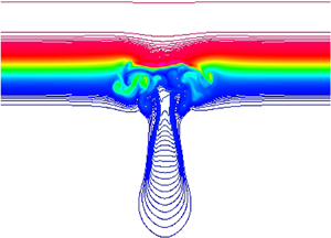
The comparison between the contours in $x_1\text {-}x_2$ planes in figures 2(a) and 2(b), which are drawn to the same scale, shows that at $t=15$, the lateral spreading of the HT is greater than that of the VT. The reason for this is found in Turner (Reference Turner1960) where it is shown that after a transition period, the radius of a buoyant vortex ring should increase as $t^{1/2}$, whereas the distance between a buoyant pair of rising ‘anti-parallel’ horizontal vortices will grow as $t$.

Figure 2.

Contours of $\theta$ at $t=15$ for the (a,c) HT and (b,d) VT with $Re=500$. The contour increment is ${\rm \Delta} \theta =0.01$. The contours are coloured from blue to red for $\theta$ increasing from $0$ to $0.3$. The contours for $0.3 < \theta \leq 0.35$ are coloured black. In (a,b), the $x_2\text {-}x_1$ plane is shown at $x_3=0$, and the horizontal black dashed lines indicate the vertical level $x_1$ from which the data for the corresponding panels (c,d) are taken. Note that the image in (d) is magnified by a factor of 2 relative to that in (b) to clearly show the azimuthal asymmetry.

In figure 2(c), we see the effect on $\theta$ of the two important instabilities that act on the rising vortex pair, instabilities that are commonly seen in the contrails behind jet aircraft. In the area of blue to green contours on the outer side of each of the two primary vortices, we see variation on a scale that is small with respect to the distance between the axes of these vortices. These structures result from the so-called short-wave cooperative instability. In the area of red to black contours, there are structures that are, at least in the axial direction, much larger. These long structures are due to the incipient long-wave instability (Crow Reference Crow1970) that typically causes the two primary vortices to connect and form separate loops breaking up the parallel structure. For more on the instabilities of counter-rotating or anti-parallel vortices, see, for example, Leweke & Williamson (Reference Leweke and Williamson1998), Orlandi et al. (Reference Orlandi, Carnevale, Lele and Shariff1998), Orlandi et al. (Reference Orlandi, Carnevale, Lele and Shariff2001) and Nomura et al. (Reference Nomura, Tsutsui, Mahoney and Rottman2006). In the case of the VT, it is instability of a vortex ring that should be expected to show up in modulations of $\theta$. In figure 2(d), there is an azimuthal variation of wavenumber 2 that appears in the otherwise nearly circular $\theta$ distribution. This variation seems weak compared to the more pronounced effects of instability in the HT case. The instability growth rates and dominant wavelengths associated with the underlying vortex structure in each case will depend on geometric parameters as well as the circulation. In the case of the VT, these parameters are the radius of the ring as well as the radius of the core of the vortex that forms the ring (Widnall et al. Reference Widnall, Bliss and Tsai1974). In the case of the anti-parallel vortices of the dipole, the instabilities are similarly controlled by the radii of the cores of the two vortices and by horizontal distance between them. Apparently, in the examples provided here, the growth rate for the Widnall instability in the vortex ring case is significantly slower than that for the short-wave cooperative instability in the anti-parallel vortex pair case.

In addition to the geometrical parameters and circulation, at low $Re$ the instabilities are significantly controlled by viscosity. Here at $Re=500$ the Widnall instability produces an azimuthal mode 2 instability. At higher $Re$, higher wavenumbers can become dominant (see e.g. Shariff et al. Reference Shariff, Verzicco and Orlandi1994).

3.3. Spreading in time

In figures 1 and 2, the contour plots are all from the same time, a time that represents a stage when the thermal was fully developed. Next we will look into the evolution of both kinds of thermals. As above, we will consider a range of $Re$ in the VT case, but only the case $Re=500$ in the HT case. In order to make the figures easier to interpret, we have taken advantage of the approximate symmetries in both of these thermals to perform some spatial averaging. For the VTs, we take advantage of the approximate symmetry about the $x_1$ axis and perform an azimuthal average about that axis to produce an averaged distribution $\langle \theta \rangle$ as a function of $r=\sqrt {x_2^{2}+x_3^{3}}$ and $x_1$. For the HT, an average along the $x_3$ direction is appropriate, yielding an average as a function of $x_1$ and $x_2$. In addition, we can exploit the near symmetry of $\theta$ with respect to reflections in the $x_3\text {-}x_1$ plane to further average $\theta$ from the values on the two sides of this symmetry plane. Again, the result is denoted $\langle \theta \rangle$.

In figure 3, the evolution of $\langle \theta \rangle$ is shown by superimposing the contours of $\langle \theta \rangle$ from different times while colouring the contours according to the corresponding time in the sequence, each time associated with a different colour. Comparing the evolution of the HT with that of the VT in figure 3(b) shows that the spreading of the HT is considerably faster than that of the VT, as was already noted above. Here, we also see that associated with increased horizontal spreading is decreased vertical velocity. In both of these types of thermals, the vertical velocity is associated with self-advection of the mean vorticity structure: in the HT case, the advection of one of the vortices in the dipole by the other; in the VT case, the advection of one part of the ring by points on the other side of the ring. Thus, the further apart the anti-parallel vortices, or the wider the vortex ring, the lower is the vertical velocity. Hence, the broader HT in figure 3(a) does not reach as high by $t=20$ (blue contours) as the narrower VT of the same $Re=500$ shown in 3(b). Note also that comparing the images of the VTs among themselves, we see that there is not much difference in the width of the thermals or the height they reach at $t=20$ comparing the cases with $Re$ equal to 500 and 1000. The same can be said concerning the pair of cases with $Re$ equal to 2000 and 5000. However, comparing the pair of VTs with the low values of $Re$ (500 and 1000) with the pair with higher $Re$ (2000 and 5000), we note a significant increase in the breadth of the thermals and a decrease in the height reached at $t=20$. The presence of finer scales at the higher values of $Re$ accounts for greater mixing and subsequent spreading of the thermal. We also note that, quite paradoxically, there are fewer contours at $t=30$ (blue) in the pair of VTs at high $Re$ compared to the pair at lower $Re$, in spite of the lower constant of thermal diffusivity $\kappa$. This is a result of a higher rate of thermal dissipation due to the finer scales that arise with sufficiently high values of $Re$. We will explore the effect of increasing $Re$ on spreading and vertical velocity more quantitatively below.

Figure 3.

Superimposed contours of $\langle \theta \rangle$ at different times: $t=5$ (red); $t=10$ (yellow); $t=15$ (green); $t=20$ (blue); $t=35$ (black). The scale of the axes and the contour interval ($\Delta =0.01$) are the same in each panel. (a) HT, $Re=500$, (b) VT, $Re=500$, (c) VT, $Re=1000$, (d) VT, $Re= 2000$ and (e) VT, $Re=5000$.

3.4. The VT: mean fields and fluctuations

The comparison between figures 3(b) and 3(e) discussed above pointed out the importance of the small-scale fluctuations at high $Re$ that are not present at $Re=500$. To analyse this further, we examine some statistics of the fields in the VT simulations performed at $Re=500$ and $Re=5000$. Of particular interest will be the mean temperature $\langle \theta \rangle$ and the mean pressure $P=\langle p\rangle$, where we use the azimuthal average defined above. Contour plots of these are displayed in figure 4 along with variances of these and other quantities: the pressure variance $\langle p'^{2}\rangle$, where $p'\equiv p-P$; the temperature variance; the velocity variance $K'\equiv \langle u_i^{\prime 2}\rangle /2$; and the vorticity variance $\Omega '\equiv \langle \omega _i^{\prime 2}\rangle /2$ (with the normalizing factor of $1/2$ added for convenience).

Figure 4.

Contours of various statistical quantities at $t=18$ for (a–f) $Re=500$ and (g–l) $Re=5000$. For all fields except for $P$, the colour table has red/blue as the maximum/minimum value. This is reversed for the $P$ field. The contour increment $\Delta$ is given below each panel. (a) $\langle \theta \rangle$, $\Delta =0.005$; (b) $P$, $\Delta =0.005$; (c) $\langle \theta '^{2}\rangle$, $\Delta =0.001$; (d) $\langle p'^{2}\rangle$, $\Delta =0.002$; (e) $\Omega '$, $\Delta =0.07$; (f) $K'$, $\Delta =0.0025$; (g) $\langle \theta \rangle$, $\Delta =0.005$; (h) $P$, $\Delta =0.005$; (i) $\langle \theta '^{2}\rangle$, $\Delta =0.001$; (j) $\langle p'^{2}\rangle$, $\Delta =0.003$; (k) $\Omega '$, $\Delta =1.0$; (l) $K'$, $\Delta =0.0125$.

In figure 4(a), showing $\langle \theta \rangle$ in the low-$Re$ case ($Re=500$), we see that the thinning of the neck connecting the cap of the thermal with the wake allows the clear definition of these two regions. The dynamics behind this thinning and the separation of the two structures is described in detail by Atkinson & Davidson (Reference Atkinson and Davidson2019). Comparing figure 4(a) with the $Re=5000$ case, we see that the separation between cap and wake is less pronounced. This contrast between the laminar and turbulent cases is also evident in the panels showing the fluctuating statistics $\langle \theta ^{\prime 2}\rangle$, $\Omega '$ and $K'$.

In contrast to $\langle \theta \rangle$ and the fluctuation statistics just mentioned, the contour plots of $P$ and $\langle p'^{2}\rangle$ at both low and high $Re$ stand out because the wake appears non-existent, at least at the level of contour increment used here. The predominant pressure signal is a strong minimum (note red marks the lowest-valued contours in figure 4b,h) in the core of the vortex ring in the head of the thermal. The lowest values of $P$ coincide with the hottest part (i.e. highest values of $\langle \theta \rangle$) in the head.

Another observation is that, at $Re=500$, the contours near the peaks of the variances are not smooth and elliptical, nor are they centred on the position of either maximum $\langle \theta \rangle$ or minimum $P$. Rather, the contours near the extremum of each of the variances are more distorted than $\langle \theta \rangle$ or $P$ near their extrema, and each is in a different position with respect to that of any of the other variances. On the other hand, the generation of strong fluctuations at $Re=5000$ leads to better mixing, and consequently the regions of high variance are more similar to the regions of high $\langle \theta \rangle$ and $P$.

3.5. Using $P$ to track the thermal

Of all the fields investigated in § 3.4, $P$ seems the smoothest in the head of the thermal. Thus, the location of the minimum of the mean pressure field $P(r,x_1,t)$ may be useful in quantitatively investigating the effect of varying $Re$ on the spreading of the thermal. We define the function $P^{*}(r,x_1^{*})=P(r,x_1^{*},t)$, where $x_1^{*}(t)$ is the height of the point where $P(r,x_1,t)$ achieves its minimum value. In figure 5, we plot $P^{*}(r,x_1^{*})$ on the $r\text {-}x_1$ plane by using the data for $P^{*}(r,x_1^{*}(t))$ for the 20 discrete values of $t$ from $t=1$ to $t=20$ in unit increments. The height of highest part of each graph corresponds to $x_1^{*}(t=20)$ and is a measure of how high the thermal has risen by $t=20$. Note that the highest points reached in the $Re=500$ and $Re=1000$ cases are significantly higher than in the $Re=2000$ and $Re=5000$ cases.

Figure 5.

Contours of $P^{*}(r,x_1^{*})$ for (a) $Re=500$, (b) $Re=1000$, (c) $Re=2000$ and (d) $Re=5000$. The contour increments are ${\rm \Delta} P^{*}=0.025$. Low/high values are coloured red/blue.

In order to give a simpler quantitative measure of the rise of the thermal with time, in figure 6(a) we plot the height change ${\rm \Delta} x_1(t)=x^{*}_1(t)-x_0$, where $x_0=3$ is the initial position of the centre of the blob, versus $t$. Note that we have added data from simulations at two additional values of $Re$. For the three lower values of $Re$ (100, solid cyan squares; 500, open red squares; 750, open blue circles), the curves show the trend that laminar thermals rise more rapidly the higher the value of $Re$. For the four highest values of $Re$, the trend is the opposite – the higher the value of $Re$ the slower the rise of the thermal. To show these opposing trends in a yet simpler form, the total rise by time $t=20$ is plotted as a function of $Re$ in figure 6(b). The red data points in the plot are taken from the same data shown in figure 6(b) with the addition of values for two more $Re$. We see that the red data points rise in height with increasing $Re$ until $Re=500$, beyond which they fall. These data suggest a transition to turbulence around $Re=500$. However, we must remember that these simulations were started from the Gaussian initial condition with random perturbations. By decreasing the amplitude of the random perturbations, one can delay the onset of turbulence in any given plume, allowing a higher vertical velocity, at least during the early evolution. By adding no random element to the initial condition, we obtain the data shown as black dots in 6(b). For the span of $Re$ represented, the black curve is monotonically rising. However, the curvature beyond $Re=500$ is negative, and a peak may be expected somewhere beyond the data point at $Re=2000$. For the case $Re=750$, we have also shown two blue hollow-square data points that represent simulations for random initial perturbations of incrementally lower amplitude than that for the simulation represented by the red dot. These points suggest that one could draw a series of curves for decreasing amplitude of initial random perturbations that would converge on the black curve. We failed to obtain a data point at $Re=5000$ in the unperturbed case because our domain with $L_1=24$ proved too limited vertically. Finding the peak of the black curve will involve a new study on a larger domain and with the higher resolution needed to reach higher values of $Re$. Finally, with regard to figure 6(b), we note that the graph readily yields the mean vertical velocity for the thermal versus $Re$ if one simply divides the ${\rm \Delta} x_{1min}$ data by ${\rm \Delta} t=20$. Note that the mean velocities so obtained range from approximately 0.7 to 0.9 for the simulations with random perturbations (red dots) and from approximately 0.7 to 1 for the case without random perturbations. The magnitudes of these velocities suggest that our reference velocity $U_0\equiv \sqrt {g\beta T_m R_0}$ was an appropriate choice for this problem.

Figure 6.

The vertical and radial displacements, ${\rm \Delta} x_{1min}$ and ${\rm \Delta} r_{min}$, of the position of the minimum $P$, for the VT. (a) The vertical displacement ${\rm \Delta} x_{1min}(t)$ versus $t$ for various values of $Re$. The dashed line is a least-squares fit of $x_1(t)=\sqrt {t/k}$ to the $Re=5000$ data over the range $t\in [10, 20]$. (b) The vertical displacement at time 20 versus $Re$ (black for smooth Gaussian initial condition (IC), red for Gaussian IC with random perturbations, blue squares from two runs with intermediate amplitudes of random perturbations). (c) The position ${\rm \Delta} r_{min}$ at time 20 versus $Re$.

The lateral spreading of the thermal can be measured by the change in the radial position ($r_{min}$) of the minimum of $P$. In figure 6(c), we plot ${\rm \Delta} r_{min}=r_{min}(t=20)-r_{min}(t=0)$ versus $Re$. Here again, we see two trends: for the low values of $Re$, ${\rm \Delta} r_{min}$ decreases with increasing $Re$; and for the high values of $Re$, ${\rm \Delta} r_{min}$ increases with increasing $Re$. By comparing figures 6(c) and 6(b), we see that, as anticipated above in § 3.3, for turbulent thermals, the slowing of the vertical rise of the thermal at high $Re$ is correlated with increasing lateral spreading with increasing $Re$.

The trend in laminar thermals for the velocity of the VT to increase with increasing $Re$ was examined in detail in a recent study by Atkinson & Davidson (Reference Atkinson and Davidson2019). They note that there is an analytic formula given by Saffman (Reference Saffman1970) for the vertical velocity $V$ for a thin-cored ring for small $Re$:

(3.1)\begin{equation} V_{visc}=\frac{\chi}{4{\rm \pi} R} \left[\ln\left(\frac{8R}{\sqrt{4\nu t}}\right) -0.558\right], \end{equation}

where $R$ is the radius of the ring and $\chi$ the circulation. The main effect included in this formula compared to the case of an inviscid ring is the viscous increase of the core radius which goes as $\sqrt {4\nu t}$. For a fixed time, as $\nu$ decreases with increasing $Re$, $V$ increases, and this should hold through the entire laminar regime.

Unfortunately, we know of no such formula showing how the vertical velocity of a turbulent thermal changes with Reynolds number. Scorer (Reference Scorer1957), using dimensional analysis independent of $Re$, developed scaling laws for the change in height and width in time for turbulent VTs. These laws have proven valid in turbulent flow in laboratory experiments. Specifically, he found that the height of the thermal goes as

(3.2)\begin{equation} x_1(t)=\sqrt{t/k}, \end{equation}

where $k$ is an experimentally determined constant. Furthermore, the width of the thermal is found to obey $r=x_1(t)/n$, where $n$ is another experimentally determined constant. In the experiments, these formulas only apply in the late stages of the flow, when the thermal is fully turbulent. The origin of time in the formulas then needs to be taken as an adjustable parameter. A fit of (3.2) to our data for $t\in [10,20]$ using the origin of time and the parameter $k$ as adjustable parameters yields the dashed curve shown in figure 6(a). The fit is reasonable; however, given that the formula and our data represent curves of the same curvature and that there are two adjustable parameters, it not surprising that a good fit can be obtained. A much more thorough study would have to be performed on a larger domain to verify this scaling in the numerical simulations, and to see how it is approached asymptotically with increasing $Re$. It may be that as $Re$ increases beyond $Re=5000$ the values of $x_{1min}(20)$ and $r_{min}(20)$ will asymptote to constants as suggested by the $Re$-independent laws of Scorer (Reference Scorer1957).

3.6. Evolution of $\overline {u_1^{2}}$ and $\overline {\theta ^{2}}$: VT

In this section, we examine the evolution of the kinetic energy components $q_i\equiv \overline {u_1^{2}}/2$ (no sum) and the temperature variance $\Theta \equiv \overline {\theta ^{2}}/2$ (where the factor of 1/2 is inserted for convenience). The overline represents integration over the entire domain. The evolution equations for $q_i$ are obtained by multiplying (2.3) by $u_i$ and integrating over the entire domain. Similarly, we obtain an equation for $\Theta$ by multiplying (2.4) by $\theta$ and integrating. Since the buoyancy term appears only in the $u_1$ momentum equation in (2.3), and this is the driving force for vertical motion, we will concentrate on the evolution of the vertical component of the kinetic energy $q_1=\overline {u_1^{2}}/2$ and $\Theta =\overline {\theta ^{2}}/2$. Thus we focus on two equations:

(3.3)\begin{equation} \frac{\textrm{d} q_1}{\textrm{d} t}=-\overline{\frac{\partial u_1^{2}{u_j}}{\partial {x_j}}} -\overline {u_1\frac{\partial p'}{\partial x_1}} +\frac{1}{Re}\overline{u_1\frac{\partial^{2} u_1}{\partial {{x_j}}^{2}}} -\overline {u_1\theta }= T_1+P_1+D_1+B_1 \end{equation}

and

(3.4)\begin{equation} \frac{\textrm{d} \Theta}{\textrm{d} t} =-\overline{\frac{\partial \theta^{2}{u_j}}{\partial {x_j}}} - \overline{u_1\theta\frac{\textrm{d}\theta_0}{\textrm{d} x_1}} + \frac{1}{RePr}\overline {\theta\frac{\partial^{2} \theta}{\partial {{x_j}}^{2}}} = T_\theta+S_\theta+D_\theta . \end{equation}

Note that the first terms on the right-hand side of each equation, $T_1$ and $T_\theta$, vanish identically since they represent integrals of divergences that vanish due to the boundary conditions that we are applying. Furthermore, if there is no background stratification, $\theta _0$ vanishes identically and, hence, the second term on the right-hand side of the $\textrm {d}\Theta /\textrm {d}t$ equation, $S_\theta$, also vanishes. Thus, the $\Theta$ equation simply states that the change in time is entirely due to diffusive dissipation represented by the term $D_\theta$, which is always negative.

We investigate next the effect of varying $Re$ on the evolution of $q_i$ and $\Theta$ in the developing VT. Given the approximate symmetry of the thermal about the vertical $x_1$ axis, it is not surprising that $q_2\approx q_3$. Thus, in figure 7(a), we examine the evolution of the three quantities: $q_1$; $q_2+q_3$; and $\Theta$. Over the entire history shown, and for all $Re$ reported, the vertical component $q_1$ is significantly larger than the horizontal components $q_2$ and $q_3$. In the early evolution, at $t\approx 1$, the ratio of the vertical component of the kinetic energy to that of the combined horizontal components is about 4. This factor rises to about 8 at $t\approx 5$ before settling down after $t\approx 15$ to about 2. The highest ratio is during the period when the vorticity is rolling up to create a well-defined vortex ring as evidenced, to a certain extent, by the images of $\theta$ in yellow in figure 3. It is also interesting to note that in the later evolution, after $t\approx 10$ for the vertical component and after $t\approx 15$ for the horizontal components, the kinetic energy components are higher the lower the value of $Re$. This is in accord with our earlier discussion, following Turner (Reference Turner1960), noting that at lower $Re$ there is less spreading and, hence, higher vertical velocity. Figure 7(a) also shows that $\Theta$ decreases monotonically at all $Re$, as must be the case since there is only one source of change for $\Theta$, the dissipative term $D_\theta$ which is always negative. As with the kinetic energy, it is noteworthy that the $\Theta$ curves are lower the higher the value of $Re$. This is related to the decrease in scale of turbulent fluctuations of $\theta$ with increasing $Re$ which leads to a higher rate of dissipation $D_\theta =\overline {\theta \boldsymbol{\nabla} ^{2} \theta }/{RePr}$. This is also related to the increased entrainment of cooler fluid with increasing $Re$. This allows for the creation of intense small-scale gradients in $\theta$ that are then smoothed by thermal diffusion.

Figure 7.

For the evolution of the VT: (a) $q_1$, circles; $q_2+q_3$, squares; $\Theta$, triangles; at the four values of $Re$ indicated; (b,c) $\textrm {d}\Theta /\textrm {d}t=D_\theta$; (d,e) $\textrm {d}q_1/\textrm {d}t=B_1+P_1+D_1$, black; $B_1$, green; ${P_1}$, blue; $D_1$, red. Reynolds number $Re=$ (b,d) 500 and (c,e) 5000.

Figure 7(a) shows that the evolution of $q_i$ and $\Theta$ at $Re=500$ is similar to that at $Re=1000$, and the behaviour at $Re=2000$ is similar to that at $Re=5000$. Thus, going forward, we limit our remarks to the two extreme values: $Re=500$ and $Re=5000$. We first consider the rate of change of $\Theta$, which in this case of no background stratification is given entirely by the term $D_\theta$ in the transport equation. The evolution of this term is shown in figures 7(b) and 7(c) for the cases $Re=500$ and $Re=5000$, respectively. In both cases, the value of $D_\theta$ is initially extremely negative (not shown) because of the strong dissipation of the initial pointwise randomly generated perturbations, but it rapidly becomes less negative and reaches a local maximum at $t\approx 2$ of approximately the same value in both cases. After this time, the value of $D_\theta$ begins to become more negative rapidly. This rise in the dissipation rate results when the initial core of high temperature pushes upward within the buoyant region creating a thinning layer of high temperature gradient above it. This thin layer bends around the rising core and, during the period $4<t<6$, rolls up in conjunction with the formation of the vortex ring. During this event, the dissipation rate $|D_\theta |$ reaches a local maximum at $t\approx 5$. The maximum dissipation rate is slightly higher for the $Re=5000$ case than for the $Re=500$ case. After this time, the vortex ring formation is complete and the dissipation rate falls off at different rates in the two cases. Dissipation rates remain elevated longer in the higher-$Re$ case because of continued presence of small-scale turbulent fluctuations.

The evolution of $\textrm {d}q_1/\textrm {d}t$ and each of the non-zero contributing terms on the right-hand side of (3.3) is rather more complicated than that of the evolution of the rate of dissipation of $\Theta$. The evolution of $\textrm {d}q_1/\textrm {d}t$ is not monotonic. Instead, it exhibits some strong oscillations (black open circles in figure 7d,e). There must be a sequence of events in the evolution of the vortex structure of the thermal that is associated with this oscillation, but we have not been able to discern what that sequence is. The oscillation is particularly puzzling in light of the way the kinetic energy just increases monotonically. The similar behaviour of $\textrm {d}q_1/\textrm {d}t$ at $Re=500$ and $Re=5000$ implies that the oscillation is due to the physics of the flow and not to a resolution issue. Further detailed study of this early (i.e. before $t=15$) phase of the development of the thermal will be needed to understand this oscillation. Of the right-hand-side terms of (3.3), the buoyancy term, $B_1$ (green dots), is positive during the entire evolution and is the sole production term. In magnitude, it is larger than either the pressure term $P_1$ (blue dots) or the viscous dissipation $D_1$ (red dots). The $P_1$ term accounts for the transfer of energy from vertical to horizontal motion. The observation that $|B_1|>|P_1|$ explains the difference in magnitude of $q_1$ and $q_2+q_3$. We also find that $P_2 \approx P_3$ and that both are production terms (i.e. positive) in the budget equation for $q_2$ and $q_3$. The rate of energy dissipation $D_1$ remains relatively small during the evolution for both values of $Re$. Consistent with our observations from figure 7(a), the term $D_1$, as well as $D_2$ and $D_3$ (not shown), is larger in magnitude for the higher Reynolds number.

3.7. Vorticity visualization

3.7.1. Vertical thermals

The generation of vorticity by baroclinic torque (see Zhao et al. Reference Zhao, Law, Lai and Adams2013) can be obtained directly from (2.3) by taking the curl. We use cylindrical coordinates $(r,\phi ,z)$, where $r$ is the distance from our $x_1$ axis and $\phi$ is the azimuthal angle measured counterclockwise from the $r$ axis looking down along the $z=x_1$ axis. The torque can be written as

(3.5a–c)\begin{equation} \tau_r= \frac{1}{r}\frac{\partial \theta}{\partial \phi}, \quad \tau_\phi= -\frac{\partial \theta}{\partial r},\quad \tau_z=0.\end{equation}

Note that there is no baroclinic torque for the $\omega _z\equiv \omega _1$ component. Generation of that component is produced only by vortex stretching and tilting. For our initial condition, which is primarily a spherical distribution, there is little early production of $\omega _r$, and it remains relatively small throughout the simulation since the thermal remains approximately azimuthally symmetric. The main baroclinic production is given by $\tau _\phi$ which drives the creation of $\omega _\phi$.

We start with a spherical vortex blob of $\theta$. Then the negative radial gradients of $\theta$ generate the positive baroclinic torque $\tau _\phi$ that generates the vortex ring of positive $\omega _\phi$. The advection by the ring forces the blob into a ‘doughnut’ shape, as we see in figure 1(a), and self-advection propels the ring vertically upward. Figure 8 shows the distribution of $\omega _\phi$ in the case $Re=500$ at times $t=15$ and $t=20$. Note that for both times there are regions of negative (blue) $\omega _\phi$. These were created by baroclinic torque just as was the primary vortex ring. Once the distribution of $\theta$ has taken on the shape of a doughnut, there is a positive radial gradient of $\theta$ on the inner side (i.e. ‘hole’ side) of the doughnut ring. The positive radial gradient generates negative baroclinic torque and thus negative $\omega _\phi$, as we see just beginning in figure 8(a) at $t=15$. From $t=15$ to $t=20$ the patches of negative $\omega _\phi$ are further amplified by baroclinic torque and also advected by the primary vortex ring leading to the distribution in figure 8(b) at $t=20$. A similar thing happens in the upper part of the tail of the thermal as we also see in this figure.

Figure 8.

Contour plots of $\omega _\phi$ in the $x_3=0$ plane for the VT with $Re=500$: (a) $\omega _\phi$ at $t=15$ and (b) $\omega _\phi$ at $t=20$. Red/blue contours represent positive/negative values. The contour level increment is $\Delta =0.125$.

Figure 9(a–d) shows the contours of $\theta$ and the vorticity components, in the $Re=500$ case, at $t=15$ in the horizontal plane at the altitude where $\theta$ takes on its maximum value. From the extremal values given in the caption, we see that the magnitude of $\omega _\phi$ is much larger than that of the other two components. The original spherical distribution of positive $\theta$ generated an annulus of positive $\omega _\phi$, a rising vortex ring that by $t=15$ has entrained much of the buoyant fluid. At this stage, the distributions of $\omega _\phi$ and $\theta$ are strikingly similar. This similarity is also well documented by Atkinson & Davidson (Reference Atkinson and Davidson2019). Furthermore, they give a discussion of the generation of vorticity by baroclinic torque, and they describe in detail the early evolution of the laminar thermal as a process comprising three stages: buoyant blob; mushroom-like cap; and buoyant vortex ring. Finally, notice that figures 9(a) and 9(c) show a mode-2 azimuthal perturbation in both $\theta$ and $\omega _\phi$. This is the result of the Widnall instability that we discussed above.

Figure 9.

Contour plots at $t=15$ for the VT with $Re=500$ (a–d) and $Re=5000$ (e–h). The contour plots are made in the $x_2\text {-}x_3$ plane at the height $x_1$ where the maximum $\theta$ is located at that time. Each axis runs from $-3$ to $+3$ and is divided into ten uniform intervals. Red/blue contours represent positive/negative values. The ranges of values are: (a) $\theta \in [0,0.31]$; (b) $\omega _r\in [-0.60,0.58]$; (c) $\omega _\phi \in [-0.3,+5.7]$; (d) $\omega _1\in [-1.37,+1.23]$; (e) $\theta \in [-0.05,0.32]$; (f) $\omega _r\in [-33.3,16.6]$; (g) $\omega _\phi \in [-30.2,+18.4]$; (h) $\omega _1\in [-34.6,+30.3]$.

The visualizations at $Re=5000$ given in figure 9(e–h) confirm that at this $Re$ we are dealing with a turbulent thermal. On a background of small-scale structures, there are large-scale clumps as in the thermals in figure 1(d) and in the visualizations in the laboratory experiment by Bond & Johari (Reference Bond and Johari2010). The baroclinic torque on the small-scale fluctuations of $\theta$ in figure 9(e) leads to the positive and negative fluctuations of $\omega _r$ in figure 9(f) and $\omega _\phi$ in figure 9(g). Although there is no creation of $\omega _1$ by baroclinic torque, the field in figure 9(h) is remarkably similar to that of $\omega _\phi$ and $\omega _r$. This isotropy of the vorticity components is a further proof that we are dealing with a turbulent thermal. Contour plots of the three components of velocity (not shown) in the case of $Re=5000$ also provide interesting information. The field $u_\phi$ has a distribution very similar to the vorticity components shown here. Component $u_1$ has high positive values on the vertical axis of the thermal. The contours of $u_r$ are primarily positive, corresponding to the radial spreading of the thermal.

3.7.2. Horizontal thermals

The evolution of the HT differs from that of the VT in some significant ways. In order to make a comparison between the spreading in the vertical and horizontal thermals, we create a $P^{*}(x_2,t)$ in a manner analogous to that used in making $P^{*}(r,t)$ for the plots in figure 5. In place of the azimuthal average used in defining $P^{*}(r,t)$, here we have an average in the $x_3$ direction. Now we can compare figure 10(f) with figure 5(a), for the VT with $Re=500$. We see that over the period $1<t<20$ the HT makes far less upward progress compared to the VT. We also see that the HT spreads radially much more than the VT in that time. The main cause of this difference lies in the way the vertical and horizontal thermals first create vorticity from the original buoyancy distribution.

Figure 10.

Contour plots for the HT for $Re=500$: (a) $\theta$; (b) $\omega _1$; (c) $\theta$; (d) $\omega _2$; (e) $\omega _3$; (f) $P^{*}(x_2,t)$. The contour increment in (a–e) is $\Delta =0.3$ and the time is $t=15$. For (f), the increment is ${\rm \Delta} P^{*}=0.025$. The contour plots in (a,b,d,e) are made at the height of the point of maximum $\theta$ as indicated by the black dashed line in (c) showing the plane at $x_3=0$. (f) $P^{*}(x_2,t)$ defined in analogy with $P^{*}(r,t)$ shown in figure 5, with the average here performed in the $x_3$ direction with only the data for $x_2>0$ shown.

Due to the different geometries of the vorticity layer that is produced by baroclinic torque from the initial $\theta$ distribution, the rolling up of this layer in the spherical initial distribution case results in a vortex ring with a radius that is smaller than the distance between the two counter-rotating vortices produced by the cylindrical distribution. This results in a considerably higher vertical velocity in the ring case than in the dipolar case. We should also note that even if the radius of the ring and the distance between the two counter-rotating vortices in the dipole were the same, the structural difference results in a faster velocity for the vortex ring. The velocities of the dipole of separation $2R$ and the ring of radius $R$ are

\[ V_{dip}=\frac{\Gamma}{4{\rm \pi} R} \quad\textrm{and} \quad V_{ring}=\frac{\Gamma}{4{\rm \pi} R}\left[ \ln\frac{8R}{a}-\frac{1}{4}\right], \]

where $\Gamma$ is the circulation and $a$ is the core radius of the ring or the radius of each vortex in the dipole. If we roughly estimate $a\approx R$ and assume the $\Gamma$ is the same in both geometries, then we would have

\[ \frac{V_{ring}}{V_{dip}}\approx 2. \]

So, we see that the geometry alone can be the cause of significant speed differences. Furthermore, the difference in the vertical velocity is continually enhanced because the HT spreads more rapidly than does the VT (see figure 2).

Consider the initial condition for the HT. The gradient of $\theta$ in the $x_2$ direction is greater than that in the $x_3$ direction. As a consequence, the baroclinic generation of vorticity is larger in the $\omega _3$ component than in the $\omega _2$ component. Furthermore, as discussed above, there can be no baroclinic generation of $\omega _1$. In figure 10, we show the contour plots at $t=15$ for each component of vorticity. Although there is no baroclinic generation of $\omega _1$, we see that that component is very similar in amplitude and form to the component $\omega _2$. That suggests that at this point in the evolution, stretching and tilting are dominant in forming the small-scale structures that we see, although baroclinic production remains active. Looking at the component $\omega _3$ we see the pattern of fluctuations that is typical of the small-scale cooperative instability familiar in contrails following aircraft. The general impression drawn from these visualizations is that this flow is in a transitional rather than a turbulent regime, which is very different from the case depicted in figure 9 of the VT at $Re=5000$.

4.1. Thermocline

In a series of experiments, Richards (Reference Richards1961) explored the effect of a thermocline in changing the evolution of a VT. The experiments involved releasing a mass of dense fluid into a freshwater layer lying over a denser salty layer. A simple rule was developed for determining under what conditions a thermal is strong enough to penetrate through the layer and continue to fall indefinitely, or so weak that it cannot penetrate at all. Here, we examine the interaction of both vertical and horizontal thermals with a thermocline. Our goal is to illustrate the type of vortex structures that are produced by the interaction. We will consider only weak thermals, that is, thermals that do not penetrate the thermocline, since in that case the production of the secondary vortex structures that we want to consider is most pronounced. Our focus is on the $Re=500$ case so that the essential vortex dynamics of the interaction will not be obscured by the generation of small scales as is the case at higher $Re$. The results will provide the kind of information about the vortex dynamics of the interaction that is difficult to obtain from laboratory experiments. For these simulations, the initial conditions are the same as in the previous simulations. The only thing that has changed is that we have placed a thermocline in the path of the thermal.

The thermocline that we use is a transition layer with a hyperbolic tangent profile connecting two uniform layers:

(4.1)\begin{equation} {\theta_0}=\theta_L+\frac{{\rm \Delta}\theta}{2}\left(1+\tanh \frac{x_1-x_c}{D}\right), \end{equation}

where ${\rm \Delta} \theta \equiv \theta _H-\theta _L$. The centre of the thermocline is defined by $x_c$ and the vertical thickness of the thermocline is controlled by $D$. In the simulations presented below, we set ${\rm \Delta} \theta =1.2$, a value sufficiently high to make the temperature in the upper layer hotter than that in the unperturbed blob, thus making penetration into the upper layer minimal. We set the centre of the thermocline at $x_c=12$ and take take $D=2/3$, making the thermocline temperature gradient strongest in the region from $x_1=11$ to $x_1=13$. With these settings, the gradient $\textrm {d}{\theta _0}/\textrm {d}x_1$ in the middle of the thermocline is 0.9. Therefore, the maximum of the Brunt–Väisälä frequency $N_{max}=\max \sqrt {{\textrm {d}\theta _0}/{\textrm {d}x_1}}$ is approximately 0.95, corresponding to an oscillation period of approximately $T_{min} = 6.6$. In a background stratification of uniform density gradient, this would be the shortest period possible for an internal gravity wave. As previously, the Gaussian blob is initially centred at $x_1=3$, putting it at 9 units (that is $9R_0$, dimensionally) below the centre of the thermocline.

4.2. Vertical thermal blocked by a strong thermocline

We begin with the case of the VT. The total temperature $\theta _T\equiv \theta + \theta _0$ at $t=15$ is plotted in figure 11 in the case with $Re=500$. At this time, the head of the VT is embedded in the thermocline and is strongly distorting it. Along the vertical axis of the thermal, the relatively cooler fluid at the bottom of the thermocline has been pushed upward toward the hotter levels above, creating a cap of high gradient of $\theta _T$. To the right and left of the central vertical axis of the thermal, we see the closed circular contours of $\theta _T$ that identify the vortex ring that has driven the thermal into the thermocline. Just to the right and left of this vortex ring, the stratified fluid of the thermocline is being pulled downward and is being wrapped around the vortex ring. The net effect is an arc of high gradient of $\theta _T$ on top of and surrounding the vortex ring.

Figure 11.

Contours of the total temperature $\theta _T=\theta _0 + \theta$ at $t=15$ in the $x_1\text {-}x_2$ plane at $x_3=0$. Contour increments are $\Delta =0.05$.

As the thermal continues to impinge on the thermocline, an interesting sequence of vortex dynamics occurs. From $t=15$ to $t=20$, there is repeated generation of secondary vorticity structures that interact with the original, that is primary, vortex ring and with the other secondary vortex structures in such a way as to break up and disperse the thermal horizontally. This sequence of vortex events is illustrated by the contour plots of $\omega _\phi$ shown in figure 12. We have seen in figure 11 that when the thermal encounters the thermocline, the contours of $\theta _T$ are bent around the primary vortex ring. At the left and right edges of the primary vortex ring, this produces strong horizontal, in other words radial, gradients of $\theta$. The strong positive radial gradient $\partial \theta /\partial r$ implies a negative baroclinic torque, which creates the negative (blue) layer of azimuthal vorticity $\omega _\phi$ on the outside of the vortex ring, as seen in in figure 12(a). In this plot, the circulation is clockwise/counterclockwise around a region of negative (blue) $\omega _\phi$ located on the left/right side of the vertical axis of the thermal. Thus, the negative (blue) $\omega _\phi$ bent around the vortex ring in figure 12(a) opposes upward vertical motion along the vertical axis and in so doing brings the thermal's rise to a halt.

Figure 12.

The collision of the VT with the thermocline for the case $Re=500$. Contours of $\omega _\phi$ with increments $\Delta =0.5$ (red, positive; blue, negative): (a) $\omega _\phi$ at $t=15$; (b) $\omega _\phi$ at $t=16$; (c) $\omega _\phi$ at $t=17$; (d) $\omega _\phi$ at $t=20$. The horizontal green lines are drawn at $x_1=11$ and $x_1=13$ to indicate the approximate vertical extent of the thermocline centred at $x_1=12$. The grey line indicates the line $r=0$ in cylindrical coordinates. It is also the vertical axis of the thermal.

Furthermore, in figure 12(a), we see that the lower part of the region of negative $\omega _\phi$ has begun to roll up into a circular vortex structure on both the left and right side of the thermal. These negative (blue) $\omega _\phi$ circular regions then begin to interact strongly with the positive (red) vorticity in the tail of the thermal as we see at $t=16$ in figure 12(b). By $t=17$, the secondary negative vorticity, located below the lower green line in the figure, has essentially separated from the region of negative vorticity lying above the primary (red) vortex ring, and is causing the vorticity in the tail of the thermal to roll up as we see in figure 12(c). This interaction has produced, in the area below the lower green line, two dipole structures, one to the left and one to the right of the central vertical axis of the thermal. At the same time, this figure shows that the remaining part of the negative (blue) $\omega _\phi$ has begun to roll up near the primary vortex ring (red), leading to the creation of two dipolar structures just above the lower green line, again one to the left and one to the right of the central vertical axis of the thermal. Such dipolar structures move by self-advection. Consider for example, the rightmost dipolar structure in figure 12(c). The positive/negative $\omega _\phi$ in that dipole causes clockwise/counterclockwise motion around itself. Thus the positive part of the dipole propels the negative part to the right and downward and the negative part propels the positive part in that same direction. Hence, this dipolar structure will move off as a whole downward to the right. The result of this self-propagation of the dipolar structures is seen at $t=20$ in figure 12(d). The four dipolar structures discussed in relation to figure 12(c) have separated as they moved away from the central vertical axis of the thermal. Each circular vortex structure in each of these dipoles in the full three-dimensional field is just the cross-section of a vortex ring that encircles the central vertical axis of the thermal. As the dipoles move laterally away from the vertical axis of the thermal, the diameter of the rings that make them up increases and the cross-sectional area of those rings decreases to conserve circulation. Thus, the cross-sectional size of the vortices making up the dipoles shrinks, at least until long-term viscous effects eventually dominate. Also, we note that new vortex structures continue to be generated by baroclinic torque and that the interaction of all the different vortex structures in the field creates strain on each of the structures that tends to shear them out and break them up during the lateral spreading of the thermal. This interaction has similarities with that described by Orlandi & Verzicco (Reference Orlandi and Verzicco1993) of vortex rings impinging solid (i.e. no-slip) walls, which involves the creation of vorticity patches on a wide range of scales leading to a rapid destruction of the initial ring vortex structure. In that case, the secondary vorticity is not created by baroclinic torque, but rather by the no-slip condition at the wall. This process also has similarities to the vortex dynamics observed in the inertial instability of vortices (see e.g. Kloosterziel, Carnevale & Orlandi Reference Kloosterziel, Carnevale and Orlandi2007).

Another important point to make is that the induced motion created by the dipoles discussed above results in a wave that propagates outward from the vertical axis of the thermal on the isolevels of $\theta _T$ in the thermocline. The obvious effect of the four main dipoles seen in figure 12 is to advect fluid downward and laterally away from the vertical axis of the thermal. A more subtle effect is that between these dipoles the induced flow is upward. For example, the space between the two dipoles lying below the green line on the right-hand side of the vertical axis of the thermal is bounded by a positive (red) vortex on the right and a negative (blue) vortex on the left. The circulation around both of these vortices is such as to advect the fluid between them upwards and towards the vertical axis of the thermal. A similar argument can be made for the pair of dipoles to the left of the vertical axis of the thermal. Next consider the pair of dipoles closest to the vertical axis of the thermal and just below the lower green horizontal line: one dipole just to the left of the vertical axis, the other just to the right. The space between these two dipoles is bounded by a positive vortex on the right and a positive vortex on the left (in other words by the two opposing sides of a secondary positive vortex ring that we see here in cross-section). The induced flow, as with the original primary vortex ring, is upward along the axis of the thermal. The combined action of all these updrafts and downdrafts will create an outwardly propagating wave on the isosurfaces of $\theta _T$ in the thermocline. It is interesting from this point of view to see the association of downward-propagating dipoles with the troughs of the wave and the upward-travelling tail ends of the dipoles with the peaks.

The effect of the vortex interactions discussed above on the distribution of $\theta$ is illustrated in figure 13. The sequence of times in this figure is the same as in figure 12. In figure 13(a), we see the large central dome of negative $\theta$ that results from the action of the primary vortex ring pushing fluid up along the $r=0$ axis. The layer of negative $\omega _\phi$ generated by baroclinic torque that is seen in figure 12(a) has a circulation that tends to force flow in the downward direction along the $r=0$ axis. This then drives the fluid back down along that axis, and by $t=20$ we see that in figure 13(d) the sign of $\theta$ above the thermal has reversed. We also see in that figure that the four main dipoles discussed in figure 12(d) are transporting relatively warm fluid into the lower layer. In the negative (blue) layer of $\theta$ just above the lower green line, we see the wave-like effect of the alternating updrafts and downdrafts associated with the dipoles as discussed above.

Figure 13.

The collision of the VT with the thermocline for the case $Re=500$. Contours of $\theta$ with increments $\Delta =0.025$ (red, positive; blue, negative): (a) $\theta$ at $t=15$; (b) $\theta$ at $t=16$; (c) $\theta$ at $t=17$; (d) $\theta$ at $t=20$. The horizontal green lines are drawn at $x_1=11$ and $x_1=13$ to indicate the approximate vertical extent of the thermocline centred at $x_1=12$.

The radial propagation of the wave in the thermocline can be better appreciated in the contour plots of $\theta$ plotted in the horizontal plane at $x_1=12$, that is, in the ($x_2\text {-}x_3$) plane lying in the centre of the thermocline, as shown in figure 14. The sequence of times shown is not the same as in figures 12 and 13, but was chosen to give a better idea of the propagation of the wave in the middle of the thermocline. When the head of the thermal has just penetrated into the thermocline, the extent of the perturbation of $\theta$ is relatively compact radially (see figure 14a), and the pattern is relatively simple mainly showing negative $\theta$ in the central region surrounded by positive $\theta$. By time $t=20$ the sign of theta in the centre has reversed and the central region is now surrounded, more or less, by two annuli of alternating sign.

Figure 14.

The interaction of a VT with a thermocline for the case $Re=500$. Contours of $\theta$ (in the $x_2$–$x_3$ plane at $x_1=12$) with increments ${\rm \Delta} \theta =0.025$ (red, positive; blue, negative): (a) $\theta$ at $t=15$; (b) $\theta$ at $t=17$; (c) $\theta$ at $t=18$; (d) $\theta$ at $t=20$.

The form and progress of the wave may be more easily assessed quantitatively in a plot of $\theta$ on a horizontal line in the middle of the thermocline (i.e. at height $x_1=12$). In order to show the propagation of the wave without distortions triggered by an initial random disturbance, the data shown in figure 15 were produced from simulations that used the Gaussian initial condition with no added random perturbations. We show results for both the $Re=500$ and the $Re=1000$ cases. Considering the $Re=500$ case, we see that at $t=14$, the perturbation mainly consists of a negative region confined between $x_2=-2$ and $x_2=+2$. By $t=30$, the wave occupies the entire domain $-6 \leq x_2 \leq +6$. Note also that the sign of $\theta$ in the central region reverses three times in the interval $14\leq t \leq 30$, representing approximately one-and-a-half cycles of oscillation. The sequence is similar for the $Re=1000$ case except that there are four reversals in the oscillation of the sign of $\theta$ in the central region. The wave periods represented by these two cases are respectively $T_\Omega \approx 10.7$ and $T_\Omega \approx 8$. Observation of a longer period of oscillation in both cases would be necessary to make these estimates more precise, but this was not possible given the limits imposed by the domain size. Both of these periods are longer than the minimum internal wave period $T_{min}=6.6$ based on the Brunt–Väisälä frequency $N(x_1)$ in the middle of the thermocline, as discussed in § 4.1.

Figure 15.

Waves produced on the thermocline during the collision of the VT in the case without initial random perturbations for (a) $Re=500$ and (b) $Re=1000$. Values of $\theta$ on the line passing through the point $(x_1=12,x_3=0)$ in the $x_2$ direction for nine different times from $t=14$ to $t=30$ with ${\rm \Delta} t=2$ between each curve. The value of $\theta$ is incremented by $0.5$ in going from one curve to the next in this sequence of times.

In an axisymmetric study of VTs, Lane (Reference Lane2008) investigated the collision of a VT with a thermocline. He too observed the oscillation in the sign of the central region and identified the basic mechanism involving generation of opposite signed vorticity by baroclinic torque that we discussed above. His results also show multiple small-scale structures including dipoles that form in the thermocline as the wave propagates away from the thermal. The work presented here goes beyond that by examining the fully three-dimensional case of the impact of the VT with the thermocline and examining in detail the dynamics of the dipoles formed during the collision.

Note that in figure 15 there is much more fine-scale structure on the curves in the $Re=1000$ case than in the $Re=500$ case. For the case with random initial perturbations added to the Gaussian, there is even more small-scale structure than in the smooth initial condition case, as one would expect. We have run such a case at $Re=1000$ and present the results here for the time $t=20$ in figure 16. The contour plots in the cross-sections shown in figure 16(a–c) can be compared directly to their counterparts at $Re=500$ in figures 12(d), 13(d) and 14(d). Given the complexity of the plots in the $Re=1000$ case, one can appreciate how difficult it would be to follow the details of the vortex dynamics and wave generation and propagation at that or higher $Re$. Thus, most of what we have done in this section has focused on the $Re=500$ case.

Figure 16.

The VT collides with the thermocline in the case $Re=1000$: (a) $\omega _\phi$ at $t=20$ in the $x_2\text {-}x_1$ plane at $x_3=0$ (contour increments are $\Delta =0.25$); (b) $\theta$ at $t=20$ in the $x_2\text {-}x_1$ plane at $x_3=0$ (contour increments are $\Delta =0.5$); (c) $\theta$ at $t=20$ in the $x_2\text {-}x_3$ plane at $x_1=12$ (contour increments are $\Delta =0.025$). Red/blue contours indicate positive/negative values. The horizontal green lines in (a,b) are drawn at $x_1=11$ and $x_1=13$ to indicate the approximate vertical extent of the thermocline centred at $x_1=12$.

4.3. Horizontal thermal collides with a strong thermocline

In figure 17, we show the evolution of the vorticity field for the case of the HT, with and without the thermocline. The vorticity component $\omega _3$ for the case without a thermocline at $t=20$ is shown in 17(a). Interestingly, we see that even in a region with no background stratification, there is the development of thin layers with alternating sign of $\omega _3$ near each of the two primary vortices of the vortex dipole. This is related to a similar effect seen above in the case of the VT and discussed in relation to figure 8, and can similarly be explained here in terms of generation of vorticity by baroclinic torque and subsequent advection of that vorticity. In the initial condition, we began with one horizontal tube of hot fluid. Baroclinic torque, stemming from the horizontal gradient of $\theta$, then created two primary opposite-signed vortex tubes, one on each side (right and left) of the original column of hot fluid. That dipolar vortex structure then divided the original column of hot fluid into two horizontal columns of hot fluid. To the right and left of each of these daughter columns, vorticity will be produced again via baroclinic torque. On one side of each, the vorticity will be of the same sign as in the core and simply add to it, while on the other it will have the opposite sign. That opposite signed vorticity will be advected around the primary vortex closest to it creating those layers of opposite sign seen in figure 17(a,b).

Figure 17.

The interaction of a HT with a thermocline for the case $Re=500$. The thermocline extends approximately from $x_1=11$ to $x_1=13$. Contours of $\omega _3$ are shown with increments ${\rm \Delta} \omega _\phi =0.2$ (red, positive; blue, negative): (a) $\omega _3$, HT without thermocline, $t=20$; (b) $\omega _3$, HT without thermocline, $t=30$; (c) $\omega _3$, HT with thermocline, $t=20$; (d) $\omega _3$, HT with thermocline, $t=30$.

For the case with thermocline shown in figure 17(c,d), the interaction of the HT with the thermocline appears retarded with respect to that shown for the VT case in figure 12(b,c). This is a result of the relatively slow propagation of the HT and the large separation between the primary vortices by the time they collide with the thermocline. In figure 17(d), at $t=30$, the same process appears at work that was already evident at $t=15$ in the VT case. Unlike the evolution in the VT case, here the opposite signed vorticity produced above each primary vortex joins with that primary vortex to produce a large-scale dipole that does not break up into smaller dipoles. The pair of dipoles that result here are oriented so as to propagate horizontally away from each other. Note that in this right-handed system, the $x_3$ axis is into the page, and, therefore, the circulation around positive/negative (i.e. red/blue) $\omega _3$ in the figure is clockwise/counterclockwise. By $t=30$, the dipoles are moving away from the thermocline, each following an arc determined by the relative strength found in the primary and secondary vortices. This scenario is very similar to that in the collision of a dipole with a no-slip wall (see e.g. Orlandi Reference Orlandi1990). In that case, the secondary vorticity is created by the roll-up of the viscous boundary layer, in contrast to this case where it is produced by baroclinic torque. Another very analogous case is given in Carnevale, Velasco Fuentes & Orlandi (Reference Carnevale, Velasco Fuentes and Orlandi1997) where we see a dipole collide with a free-slip wall, but with secondary vorticity produced by topographic stretching. Independent of the method of secondary vorticity production, the trajectories of the vortices are very similar in each of these scenarios.

The contour plots of $\theta _T$ and $\theta$ for the HT collision with the thermocline are shown in figure 18. The plots of $\theta _T$ (figure 18a,c) nicely illustrate the degree to which the thermocline is perturbed in this case. These can be compared with the plot of $\theta _T$ in the VT case shown in figure 11. Clearly the penetration is shallower and much delayed in the HT case. We will not go into detail about the way this collision initiates an internal wave on the thermocline as we did in the VT case. We will, however, note that in figure 18(b), on the horizontal line at $x_1=12$, going from left to right one sees four reversals in the sign of $\theta$. Furthermore, the sign of $\theta$ at $x_2=0$ on this line reverses by $t=30$ as seen in figure 18(d).

Figure 18.

Results at $t=20$ and $t=30$ from the thermocline penetration experiment for a HT with $Re=500$. The plots show both the total temperature $\theta _T=\theta + \theta _0$ and the temperature perturbation $\theta$. Contour increments are $\Delta =0.01$: red, positive; blue, negative. The fields are shown in the $x_1\text {-}x_2$ plane at $x_3=0$: (a) $\theta _T$ at $t=20$; (b) $\theta$ at $t=20$; (c) $\theta _T$ at $t=30$; (d) $\theta$ at $t=30$.

4.4. Evolution of $q_i$ and $\Theta$ with thermocline: VT and HT

In the presence of stratification, in the Boussinesq approximation, the potential energy of the flow is given by

(4.2)\begin{equation} \mathit{PE}=\frac{1}{2}\int \frac{\theta^{2}}{N^{2}} \,\textrm{d}x_1\,\textrm{d}x_2\,\textrm{d}x_3. \end{equation}

The inviscid conservation kinetic energy $q_1+q_2+q_3$ plus this potential energy can be confirmed using (2.3), (2.4) and (2.5). Although the variance $\Theta$ is not equivalent to potential energy, it behaves somewhat analogously because its sources $B_1$ and $S_\theta$ in (3.3) and (3.4) are similar to those that drive changes in the potential energy.

Figure 19(a) shows the evolution of the kinetic energy components $q_1$ and $q_2+q_3$, and $\Theta$ (green curves) for the VT encountering the thermocline. These can be compared to the corresponding curves from the unstratified case (red curves). In the early development of the thermal, before it encounters the thermocline, roughly before $t\approx 8$, the behaviour of $q_i$ and $\Theta$ is very similar to that in the simulation without the thermocline. As the vortex ring encounters the thermocline, the thermocline is pushed up increasing $\Theta$. The thermal responds by slowing. The simultaneous increase of kinetic energy (particularly the $q_1$ component) and decrease of $\Theta$ is clear for the period $9<t<14$. After $t\approx 10$, there is an oscillation in the green curves in figure 19(a). This oscillation is more clearly evident in the black curves in figure 19(c,e). The period of the oscillation is ${\rm \Delta} t\approx 7$. This is consistent with internal waves since it is longer than the minimum period $T_{min}=6.6$ for internal waves on our thermocline, as we noted in § 4.1. This oscillation seems distinct from that which is evident before $t\approx 10$ on say the $P_1$ (blue) curve in figure 19(e). That earlier oscillation has a period of ${\rm \Delta} t\approx 4$ which is similar to what we saw in the early phase of the evolution of the thermal in the unstratified case (see figure 7d). If our estimate for the minimum period for an internal wave based on the maximum value of $N$ in the thermocline is valid, this shorter-period oscillation before $t\approx 10$ is unrelated to internal wave activity.

Figure 19.

Evolution of $q_1$, $q_2+q_3$ and $\Theta$ and their source terms for $Re=500$: (a) Vertical thermals: top two curves, $q_1$; middle two curves, $q_2+q_3$; bottom two curves, $\Theta$ (green, with thermocline; red, no thermocline). (b) Horizontal thermals: top two curves, $q_1$; middle two curves, $q_2+q_3$; bottom two curves, $\Theta$ (green, with thermocline; red, no thermocline). (c) Vertical thermal with thermocline: $\textrm {d}\Theta /\textrm {d}t=S_\theta +D_\theta$, black; $S_\theta$, green; $D_\theta$, red. (d) Horizontal thermal with thermocline: $\textrm {d}\Theta /\textrm {d}t=S_\theta +D_\theta$, black; $S_\theta$, green; $D_\theta$, red. (e) Vertical thermal with thermocline: $\textrm {d}q_1/\textrm {d}t=B_1+P_1+D_1$, black; $B_1$, green; ${P_1}$, blue; $D_1$, red. (f) Horizontal thermal with thermocline: $\textrm {d}q_1/\textrm {d}t=B_1+P_1+D_1$, black; $B_1$, green; ${P_1}$ blue; $D_1$, red.

In figure 19(c), the evolution is dominated by the variation of the curves after time $t=10$. This contrasts with the behaviour in the unstratified flow (see the corresponding figure 7b) where the evolution before $t=10$ dominated. But note that the amplitude of the variations in the unstratified case were more than 30 times smaller than in this case with thermocline. The early variations before $t=10$ are not appreciable on the scale of figure 19(c). In this figure, the large and rapid increase in $S_\theta \equiv -\overline {u_1\theta \, \textrm {d}{\theta _0}/\textrm {d}x_1}$, starting around $t=10$, corresponds to the rise of $\Theta$ seen in figure 19(a). The subsequent plunge of $S_\theta$ to very negative values makes it much more important than the dissipation $D_\theta$ in bringing $\Theta$ rapidly down again.

For the HT case shown in figure 19(b), we ran the simulation to $t=45$, much longer than in the VT case, because the HT rises more slowly, as already discussed. Note that the scale of the vertical axis in 19(b) is about a factor of 10 larger than in 19(a). This is due to the increase in energy of the HT with its extension in the $x_3$ direction. So, here we focus only on the relative changes. Note that $\Theta$ does not have a rapid period of growth in this case as opposed to the VT case. This is because the HT does not penetrate as far into the thermocline as the VT and thus does not push the isopycnals as far up.

Next consider figure 19(d) showing the production terms for $\Theta$ in the HT case. Note that the vertical scale of figure 19(d) is smaller than that of figure 19(c), corresponding to the shallowness of the penetration of the HT into the thermocline compared to the VT case. After $t\approx 10$, the relative balance between dissipation $D_\theta$ (red curve) and $S_\theta$ (green curve) results in the total $\textrm {d}\Theta /\textrm {d}t$ (black curve) remaining relatively small and the size of $\Theta$ after $t\approx 10$ remaining relatively constant (see figure 19b). Finally, note that the period of oscillation in $S_\theta$ is ${\rm \Delta} t\approx 15$ which is about double that in the VT case. It is not clear to us why there is this difference in period. It may be related to the size and shape of the thermal when it hits the thermocline since that would affect the wavelengths excited. For horizontally propagating internal waves on a uniform background gradient of temperature (i.e. a background of uniform $N$), the frequency would be $N$, independent of wavelength. We are not aware of any analytical studies of wave propagation on a hyperbolic tangent thermocline, so we can only speculate at this point that the frequency difference is an effect of the different wavelengths and/or symmetry of the waves.

The budgets for $q_1$ in figure 19(e,f) are more complex than their counterparts for the evolution of $\Theta$. It seems the generation term $P_1$ (blue) is forced into an oscillation $180^{\circ }$ out of phase with $B_1$ (green). The oscillations of $B_1$ during the strong interaction of the VT after $t\approx 10$ with a period longer than $T_{\textit{min}}$ are consistent with internal waves. Since we have seen that oscillations in the kinetic energy production terms can occur even in the case with no thermocline, even while the kinetic energy is monotonically increasing (see figure 7), we can only say here that the oscillations in the case with thermocline are consistent with internal waves and with the evidence of waves that we presented above in the form of contour plots and graphs of vorticity and $\theta$ within the thermocline. Note also that the strongly negative $P_1$ (blue) in figure 19(f) at $t\approx 15$ finally overcomes the positive production $B_1$ (green) to force the decay of $q_1$ from its peak in figure 19(b) in the stratified case (green line) compared to the neutral environment case (red line). However, the continued decay of $q_1$ after $t\approx 23$, after which $P_1\approx 0$, is due to $B_1$ turning negative as well as the effect of the uniformly negative $D_1$ (red).

Internal wave radiation away from the site of the collision of the thermal with the thermocline on an infinite domain would show up as a loss of energy from the local interaction volume. We could not, however, quantify this kind of loss of energy because this would require developing a numerical scheme with some sort of ad hoc radiation condition or sponge layer at the boundaries of the domain. This is left for possible future exploration.