


1. Introduction
Gravitational mass flows in general appear in different forms, ranging from continuum motion such as fluvial processes to particle governed motion like rock falls. Snow avalanches in particular show various flow types including dense basal flow of snow granules or destructive powder snow flows (Sovilla and others, Reference Sovilla, McElwaine and Louge2014; Köhler and others, Reference Köhler2018a), going beyond the powder/dense flow avalanche dichotomy (Faug and others, Reference Faug, Turnbull and Gauer2018). Experiments to access flow dynamics at the particle level have been limited to the analysis of avalanche deposits (Bartelt and McArdell, Reference Bartelt and McArdell2009) or to laboratory experiments that reveal interesting details on the granular behaviour (Steinkogler and others, Reference Steinkogler, Gaume, Löwe, Sovilla and Lehning2015a) and surprising temperature dependence of snow (Fischer and others, Reference Fischer, Kaitna, Heil and Reiweger2018). On a field scale, some of the standard approaches of motion tracking are prone to fail in snow avalanches (e.g. limited visibility for photogrammetry or antenna orientation and signal attenuation by snow for GNSS methods). So far, in situ inertial measurements have therefore been limited to chute experiments, providing estimates on speed and position along a predefined chute topography (Vilajosana and others, Reference Vilajosana, Llosa, Schaefer, Surinach and Vilajosana2011).
An improved knowledge of internal particle dynamics in snow avalanches is desirable, not only to better understand the governing processes and to acquire data for model evaluation, but also for a reliable prediction of single particle motion. With this information, scientists and engineers may have a new opportunity to identify and interpret impact pressures that cannot directly be examined by classical approaches (Faug, Reference Faug2015; Sovilla and others, Reference Sovilla2016; Kyburz and others, Reference Kyburz, Sovilla, Gaume and Ancey2022a, Reference Kyburz, Sovilla, Gaume and Ancey2022b) or to predict the transport and corresponding burial location of avalanche victims. During the past few years, several researchers have developed independently the idea to apply methods of inertial navigation for a motion tracking in gravitational mass movements. Related endeavours aim at reliable motion data including particle velocities, inertial effects (centrifugal forces) and vertical motion relatively to the terrain (due to buoyancy and segregation). The basic idea is to record translational acceleration and angular velocity components, which, in principal, allow to determine a trajectory via time integration. Most recently, the suitability of inertial navigation devices in combination with observations through unmanned aerial vehicles has been investigated for the recording of rockfall trajectories, also providing a review of related approaches (Caviezel and others, Reference Caviezel2019). Furthermore, Dost and others (Reference Dost, Gronz, Casper and Krein2020) investigated the potential of inertial sensor devices in laboratory landslide experiments, introducing the Smartstone probe v2.0 as a device to measure movement characteristics of single clasts. They highlight how physical movement characteristics can be derived from the measured and calibrated data and the potential of a 2D and 3D visualization of the paths a clast took during the movement and how these visualizations allow for an easy recognition of complex motion patterns. These developments allowed to investigate the influence of shape and mass in rockfall experiments (Caviezel and others, Reference Caviezel2021) or in depth motion analysis utilizing rockfall video trajectories (Noël and others, Reference Noël2022).
Inertial navigation systems are widely used in engineering as well as everyday life applications such as naval, aircraft and, in particular, drone navigation, positioning in cell phone applications and many others. Most modern inertial navigation systems belong to the class of so-called strap-down devices (Groves, Reference Groves2008). The method of strap-down inertial navigation is based on the measurement of accelerations and angular velocities by means of sensor clusters ‘rigidly’ linked to a moving object of interest.Footnote 1 Corresponding devices are commonly called ‘inertial measurement units’ (IMU). If earth's magnetic field is detected in addition, the term ‘motion processing unit’ is preferred by some authors. An extensive overview of accelerometer, gyroscope and magnetometer technology is given in Titterton and Weston (Reference Titterton and Weston2004).
Position and orientation data are obtained by numerical integration of the kinematic differential equations (navigation equations) relating the time derivatives of position and orientation (angular) parameters with the acceleration and angular velocity components (Groves, Reference Groves2008). A common approach to improve the accuracy of the integration procedure is to apply stochastic estimation techniques, such as Kalman filtering (Simon, Reference Simon2006). Such methods rely on a deterministic model predicting the system dynamics, a measurement model and on specific assumptions related to the stochastic properties of the measurement error. For tracking applications, the system as well as the measurement model are non-linear, which leads to complex implementations involving a reasonable number of tuning parameters, a proper adjustment of which is often difficult. However, a beneficial peculiarity of the tracing problem is that the non-linearity originates from the angular motion only and that the related kinematic differential equations can be integrated independently from the state variables of the translational motion.Footnote 2 A commonly known algorithm for the estimation of IMU orientation which avoids the complexities of non-linear state estimation has been released by Madgwick and others (Reference Madgwick, Harrison and Vaidyanathan2011). The idea is to determine the orientation increment in each time step twice: once via integration of the angular rates and once from magnetometer and/or accelerometer data. The orientation is then updated by a weighted average of both increments. The method works particularly well if no (or only small) inertial accelerations occur, i.e. if the accelerometers measure only the effect of gravity. In this case, the orientation can be determined uniquely from accelerometer and magnetometer data by solving a minimization problem. In the case of avalanche tracking, it turned out that acceleration signals are of limited use for this purpose. As long as only the magnetometer data are available for the orientation estimation, this procedure is not unique. Therefore, a new algorithm has been developed which allows to determine the sensor orientation from gyroscope and magnetometer data in a robust manner even under the rough conditions of the present application. The orientation information at each time step can then be used to transform the acceleration components to a global coordinate system, which, in turn, allows to apply a simple numerical integration scheme for the determination of velocity and position.
One of the first real-scale avalanche particle tracking experiments, which was
accompanied by Doppler radar measurements and terrestrial laser scanning (TLS), has
been performed at the Flüelapass field site in Switzerland on 23 January
2013. At this time, the experiments focused on infrared thermography and
corresponding avalanche temperatures (Steinkogler and others, Reference Steinkogler, Sovilla and Lehning2015b). Due to the lack of prior experience, multiple
prominent problems arose related to the particle tracking measurement technology
applied: Firstly, the sensor calibration has been performed under laboratory
conditions that do not sufficiently correspond to the relevant field conditions.
Secondly, the measurement range of the gyrometers has been chosen too small, which
has lead to a cut-off of angular velocity peaks at about
$\pm 360^\circ$ s−1.Footnote 3 Additionally, a technical recording
error limits the possibility of a full data integration. However, these limitations
inspired the development of corresponding workarounds, which not only allow to
deduce the desired results but in addition give rise to novel methods of sensor
calibration. These aspects are described in detail below. The main focus of this
manuscript is therefore the methodological description of the approaches and
numerical procedures, which have been developed to tackle the specific deficiencies
of the given dataset. The observed avalanche event provides a test case to assess
both, the experimental setup as well as the related methods of data processing. It
is emphasized that the present work is dealing with the evaluation of, so to say,
‘historical’ data, which have been recorded with the help of, from
today's point of view, outdated hardware. At the time of the experiment, the
combination of procedures presented here was not available, whereas attempts to
apply conventional approaches failed. Despite the technological advances of the last
years, the availability of comparable data from real-scale experiments is still
limited, such that trying to extract as many results as possible even from outdated
experiments is justified. Most recent approaches highlight the usability of
state-of-the-art hardware, investigating particle motion in avalanches with global
tracking (Global Navigation Satellite System [GNSS]) approaches (Neuhauser and
others, Reference Neuhauser, Koehler, Neurauter, Adams and Fischer2023). The article is organized as
follows: Section 2 describes the details of
the experimental procedure. It is followed by an overview of the recorded IMU data
and a qualitative assessment and interpretation (Section 3). Theory, results and assessment of a quantitative
evaluation of the IMU data based on a standard sensor calibration yielding estimates
of angular orientation, translational and rotational velocities, as well as the
sensor trajectory are given in Section 4. The
numerical procedure providing the angular orientation is specifically designed to
optimally deal with the given dataset. Motivated by a misalignment of the recovered
trajectory, a novel calibration approach is introduced, applied and assessed in
Section 5. Sections 6 and 7 summarize and
finally assess the findings, discuss their significance for the fields of avalanche
research in particular as well as for the problem of motion tracking in general and
address the lessons learned for future avalanche experiments. The standard
procedures of sensor calibration are briefly summarized and postponed to Appendix A,
since they rely on state-of-the-art algorithms. The recovery of deficient gyrometer
data is not state-of-the-art but is considered too specific to justify interrupting
the flow of argumentation in the main text and is therefore placed in Appendix
B.
s−1.Footnote 3 Additionally, a technical recording
error limits the possibility of a full data integration. However, these limitations
inspired the development of corresponding workarounds, which not only allow to
deduce the desired results but in addition give rise to novel methods of sensor
calibration. These aspects are described in detail below. The main focus of this
manuscript is therefore the methodological description of the approaches and
numerical procedures, which have been developed to tackle the specific deficiencies
of the given dataset. The observed avalanche event provides a test case to assess
both, the experimental setup as well as the related methods of data processing. It
is emphasized that the present work is dealing with the evaluation of, so to say,
‘historical’ data, which have been recorded with the help of, from
today's point of view, outdated hardware. At the time of the experiment, the
combination of procedures presented here was not available, whereas attempts to
apply conventional approaches failed. Despite the technological advances of the last
years, the availability of comparable data from real-scale experiments is still
limited, such that trying to extract as many results as possible even from outdated
experiments is justified. Most recent approaches highlight the usability of
state-of-the-art hardware, investigating particle motion in avalanches with global
tracking (Global Navigation Satellite System [GNSS]) approaches (Neuhauser and
others, Reference Neuhauser, Koehler, Neurauter, Adams and Fischer2023). The article is organized as
follows: Section 2 describes the details of
the experimental procedure. It is followed by an overview of the recorded IMU data
and a qualitative assessment and interpretation (Section 3). Theory, results and assessment of a quantitative
evaluation of the IMU data based on a standard sensor calibration yielding estimates
of angular orientation, translational and rotational velocities, as well as the
sensor trajectory are given in Section 4. The
numerical procedure providing the angular orientation is specifically designed to
optimally deal with the given dataset. Motivated by a misalignment of the recovered
trajectory, a novel calibration approach is introduced, applied and assessed in
Section 5. Sections 6 and 7 summarize and
finally assess the findings, discuss their significance for the fields of avalanche
research in particular as well as for the problem of motion tracking in general and
address the lessons learned for future avalanche experiments. The standard
procedures of sensor calibration are briefly summarized and postponed to Appendix A,
since they rely on state-of-the-art algorithms. The recovery of deficient gyrometer
data is not state-of-the-art but is considered too specific to justify interrupting
the flow of argumentation in the main text and is therefore placed in Appendix
B.
2. Experimental set-up and test procedure
To investigate the particle movement in a snow avalanche, a measuring device,
subsequently also called sensor unit, is placed in the release area
or potential flow path before the avalanche is triggered. In the course of the
experiment the sensor unit is expected to be entrained and further transported by
the moving snow and thus to resemble the particle motion in the avalanche. The
measuring device consists of several sensors, a micro controller, a data storage
unit and an electrical power supply, which are embedded in a rigid, spherical
housing (Fig. 1). The housing properties are
chosen to resemble snow granules found in avalanche deposits (Bartelt and McArdell,
Reference Bartelt and McArdell2009) with a density of
≈300 kg m−3 and a diameter of
≈16 cm (Fischer and Rammer, Reference Fischer and Rammer2010). The sensors applied involve a six-axis inertial sensor (IMU), a
three-axis magnetometer and a GNSS module. The utilized IMU (ADIS16355) is an
assembly of three accelerometers and three gyrometers aligned with three mutually
perpendicular directions and capable of measuring the corresponding acceleration and
angular velocity components, respectively. The magnetic sensor HMC1043 measures the
magnetic flux densityFootnote 4 in the same
directions (nominally). The applied GNSS module is a ublox LEA-4T-0-000 receiver.
The power supply is provided by a rechargeable battery. Data are recorded with a
sampling rate of 150 Hz and stored on an SD card. The measurement range of
gyrometers is set to a nominal value of
$\pm 300^\circ$ s−1 with a
digital resolution of 14 bit and a sensitivity of
0.0725–$0.0740^\circ$
s−1 with a
digital resolution of 14 bit and a sensitivity of
0.0725–$0.0740^\circ$ s−1 LSB−1.
The range of accelerometers is nominally ±10 g with a digital
resolution of 14 bit as well and a sensitivity of
2.471–2.572 mg. The range of magnetometers is nominally
±6 Gs with a sensitivity of
0.8–1.2 mV V Gs−1. The six
inertial sensors (gyrometers and accelerometers) are assembled in a cuboidal housing
with an edge size of approximately 23 mm. While the positioning of gyrometers
is uncriticalFootnote 5 the positioning of
accelerometers deserves a certain attention: since the three accelerometers cannot
be located at the same position, a so-called origin alignment is applied internally
by the device, such that the acceleration values refer to a defined reference point.
This reference point is depicted in (Fig.
1).
s−1 LSB−1.
The range of accelerometers is nominally ±10 g with a digital
resolution of 14 bit as well and a sensitivity of
2.471–2.572 mg. The range of magnetometers is nominally
±6 Gs with a sensitivity of
0.8–1.2 mV V Gs−1. The six
inertial sensors (gyrometers and accelerometers) are assembled in a cuboidal housing
with an edge size of approximately 23 mm. While the positioning of gyrometers
is uncriticalFootnote 5 the positioning of
accelerometers deserves a certain attention: since the three accelerometers cannot
be located at the same position, a so-called origin alignment is applied internally
by the device, such that the acceleration values refer to a defined reference point.
This reference point is depicted in (Fig.
1).
Left: Top view of the sensor
unit with opened housing. The x and y
axes of the sensor coordinate system are drawn at the geometric centre
of the spherical casing. The reference point to which the accelerations
are referred to coincides with a corner of the bottom face of the
cuboidal IMU housing. Its position vector relatively to the drawn
coordinate system is
${}^1{\boldsymbol \varepsilon }\approx [ 12\; -31\; -12] ^T$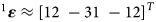 mm.
Right: Coordinate systems referred to in this work:
inertial, sensor and slope coordinate system (or
frame).
mm.
Right: Coordinate systems referred to in this work:
inertial, sensor and slope coordinate system (or
frame).

To recover the sensor unit velocity and trajectory from the recorded data (tracking), a proper calibration of IMU sensors (including magnetometers) is crucial. An overview of the standard calibration procedures applied here, can be found in Appendix A. Originally, the calibration of the three-axis accelerometer has been done on the basis of a standard six-position static test referring to earth's gravitational acceleration as a reference. To calibrate the three-axis gyrometer, constant angle rate tests have been performed utilizing a Stäubli TX2-90 industrial robot, following the methods, described by Aggarwal and others (Reference Aggarwal, Syed, Niu and El-Sheimy2008) or Stančin and Tomažič (Reference Stančin and Tomažič2014). The magnetometer calibration is performed applying Earth's magnetic field as a reference (Renaudin and others, Reference Renaudin, Afzal and Lachapelle2010). Retrospectively, it turned out that it is a certain drawback of the experimental work that the calibration procedures have not been performed in temporal and local proximity to the measurements. Since the experiment has been one of the first of its kind, a lack of appropriate experience has thus lead to some effect of misjudgement. In particular, the laboratory calibration of magnetometers proved to be inadequate: measuring Earth's magnetic field provides information about the angular orientation of the sensor unit. To this end it has to be ensured that the magnitude of the measured flux density is basically constant. If this is not the case, either (electro-) magnetic disturbances are present or the calibration of the magnetometers is wrong. Both sources of error would corrupt the evaluation of angular orientation, the knowledge of which is decisive for a proper tracking process. In the present case, an existing non-constancy of the magnetic field could be attributed to the inadequacy of the laboratory calibration and be remedied by a recalibration on the basis of the in-field data. The theoretical background and an assessment of the procedure can be found in Appendix A. The name ‘in situ calibration’ is suggested for this approach. The laboratory calibration of accelerometers also represents a source of error and can be improved by an in situ approach as well. Section 5 is dedicated to this topic.
The test site is located close to Davos in Switzerland
[46.748621$^\circ$ (N),
9.945134$^\circ$
(N),
9.945134$^\circ$ (E), WGS84]. The avalanche path is a
north-east facing slope, with an altitude difference of 600 m. Deposits of
larger avalanches typically reach a lake located at 2374 m a.s.l. at the
bottom of the slope (Fig. 2). The slope
angle ranges from
$50^\circ$
(E), WGS84]. The avalanche path is a
north-east facing slope, with an altitude difference of 600 m. Deposits of
larger avalanches typically reach a lake located at 2374 m a.s.l. at the
bottom of the slope (Fig. 2). The slope
angle ranges from
$50^\circ$ in the rock face in the upper part to
$20^\circ$
in the rock face in the upper part to
$20^\circ$ at the beginning of the run-out zone with
an average of
$30^\circ$
at the beginning of the run-out zone with
an average of
$30^\circ$ of the open slope at around 2600 m
a.s.l. The avalanche had an approximate destructive size d2 (Canadian Avalanche
Association, 2016) and was released
artificially. According to the international avalanche classification (De Quervain,
Reference De Quervain1981) avalanche 20130123 classifies as
A2B4C1D2E2F4G1H1J4, with a possible variation concerning the form of motion (mixed
type with powder part, E7).
of the open slope at around 2600 m
a.s.l. The avalanche had an approximate destructive size d2 (Canadian Avalanche
Association, 2016) and was released
artificially. According to the international avalanche classification (De Quervain,
Reference De Quervain1981) avalanche 20130123 classifies as
A2B4C1D2E2F4G1H1J4, with a possible variation concerning the form of motion (mixed
type with powder part, E7).
Overview of the test site including the main avalanche release, track and deposit, the sensor unit trajectory, as well as radar, TLS and video camera position with relative, projected distance to the avalanche.
Supplementary measurements of the avalanche event include video recordings (see
supplementary material), Doppler radar measurements, pre-event terrain
reconstruction by means of TLS and GNSS positioning of the tip of the avalanche
deposition and of the final location of the sensor unit. The Doppler radar
observations deliver a range-time diagram of the avalanche front (amongst other
information). Roughly speaking, the slope of the range-time curve equals the
velocity of the avalanche front projected onto the instantaneous radar beam (Gauer
and others, Reference Gauer2007; Rammer and others, Reference Rammer, Kern, Gruber and Tiefenbacher2007; Gauer and Kristensen, Reference Gauer and Kristensen2016). To account for the topography, radar
velocities are scaled with
$1\cos {^{-1}} \delta$ , where δ is the
angle between the slope line and the radar beam (Fischer and others, Reference Fischer, Fromm, Gauer and Sovilla2014). The range time diagram involving the
radar signal strength is presented in Figure
3. Comparing the so obtained frontal velocities with the sensor unit
velocity recovered from the IMU data helps to assess the tracking procedure and
gives further hints related to the motion of the sensor unit relatively to the
avalanche front.
, where δ is the
angle between the slope line and the radar beam (Fischer and others, Reference Fischer, Fromm, Gauer and Sovilla2014). The range time diagram involving the
radar signal strength is presented in Figure
3. Comparing the so obtained frontal velocities with the sensor unit
velocity recovered from the IMU data helps to assess the tracking procedure and
gives further hints related to the motion of the sensor unit relatively to the
avalanche front.
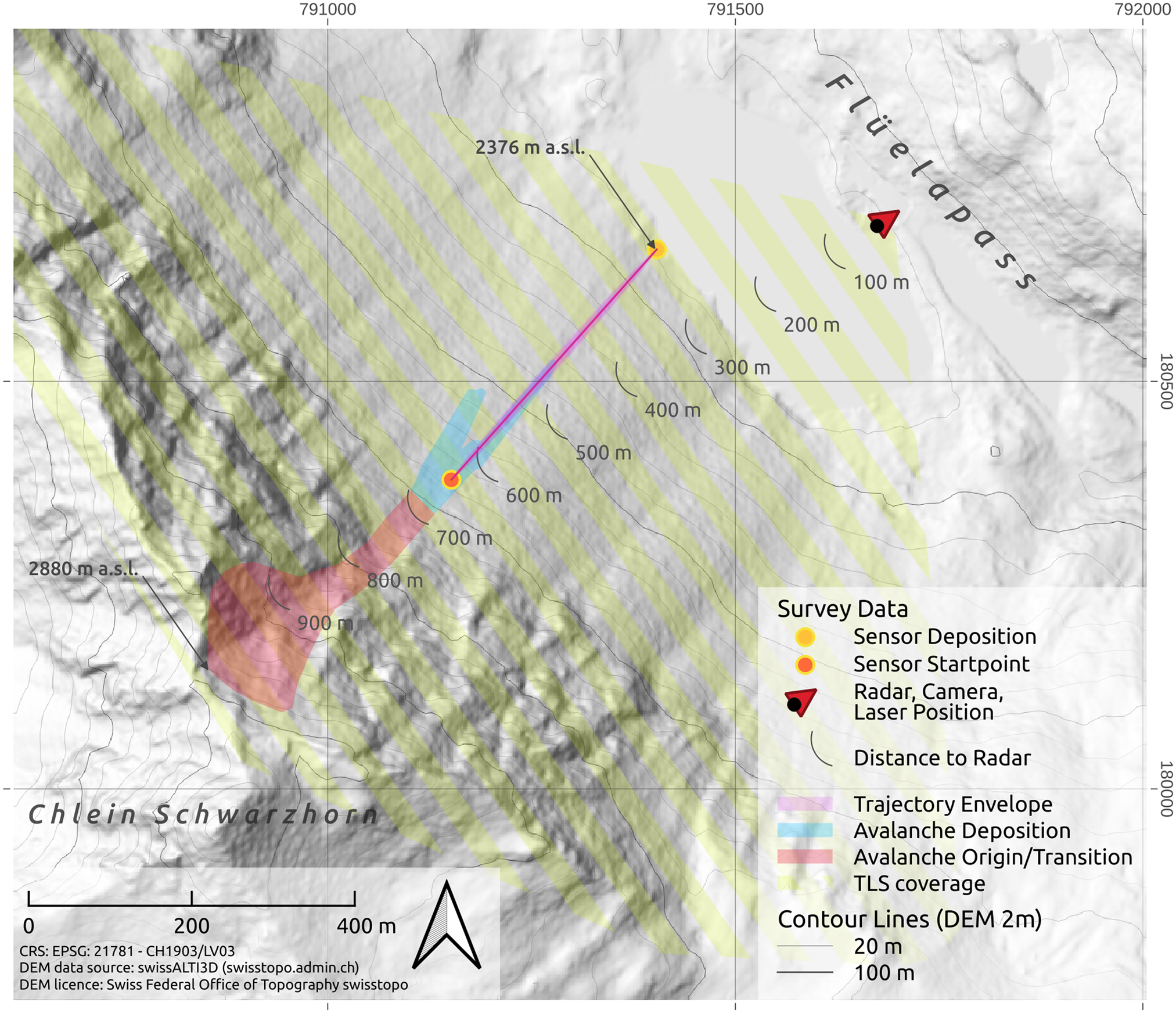
Left: Range-time diagram of the Doppler radar measurement, from which the frontal avalanche velocities can be deduced and which allows for the cross-validation of the corresponding flow regimes. The gray framed box indicates the relevant domain related to the present experiment: from entrainment of the sensor unit stillstand of the bulk of the avalanche. The signals below that box refer to individual snowballs moving further for a while. Right: The avalanche shortly before the transition from the cold-dense to the snowball regime corresponding to the steady flow phase. The sensor unit (indicated by the red circle) is about to leave the bulk of the avalanche.
After release, the avalanche quickly accelerated to velocities between 20 and 25 m s−1 and developed a small powder part. The main mass movement was characterized by a dense flow and a pronounced roll-wave activity (see Fig. 3 and the supplementary video material), showing the typical characteristics of a cold dense regime as defined in Köhler and others (Reference Köhler, McElwaine and Sovilla2018b). The sensor unit has been entrained by the avalanche in the upper part of the open avalanche track with a frontal velocity between 20 and 21 m s−1 at an approximate distance of 650–675 m from the radar device. After a steady phase, flow velocities decrease from 18 to 10 m s−1, the main avalanche body came to rest at a radar distance of 450–475 m. Up to this point (about 16 s after being entrained), the sensor unit has covered a travelling distance of 220–225 m within the dense cold regime and finally detached from the avalanche body. Together with snow fragments, remaining from the entrainment process, the sensor unit kept moving in a rolling motion within the snowball regime (Köhler and others, Reference Köhler, McElwaine and Sovilla2018b). The individual snowballs or snow wheels are visible in radar distances between 250 and 450 m, rolling down the slope with varying velocities between 7 and 13 m s−1. The rolling motion can qualitatively be reconstructed by the sensor data. The total duration of the movement was 70 s and is in accordance to the radar recordings.
The GNSS measurements were used to determine the initial and final sensor unit position with a corresponding trajectory length of ≈ 420–430 m. To obtain an estimate of the sensor unit trajectory, a straight line is assumed from the initial to the final sensor unit position, see the purple area depicted in Figure 2. The x (East) and y (North) coordinates of the starting and of the end point are obtained from the data of the GNSS module contained in the sensor housing and are averaged over a time period of several minutes. The coordinates of the tip of the avalanche deposition have been checked with the help of an external GNSS receiver. The orographic left and right boundaries of the trajectory envelope are obtained by projecting the envelope onto the terrain surface given by the TLS terrain model. The diameter of the trajectory envelope is assumed to equal the maximum width of the lower part of the avalanche deposition. The geometry of the terrain surface serves as an input for the in situ calibration and the trajectory envelope is used to assess the trajectory recovered from inertial measurements via the numerical algorithms described in this work. To account for the resolution and the accuracy of the terrain model (±0.5 m, each), the surface projection of the envelope (a rhombus, basically) is extruded (1 m in outward and 1 m in inward normal direction) to become a double wedge and is referred to as reference tube.
3. Experimental results and qualitative analysis
3.1. Overview
As already anticipated in the introduction, the measurement process has come along with some shortcomings: Firstly, the occurring angular velocities occasionally exceed the measurement range of the gyrometers and, secondly, a failure of data recording occurred approximately 9 s after the sensor unit has been entrained by the avalanche, such that reliable data are missing over a time span of about 0.5 s. The first problem can be circumvented with the help of magnetometer data. The second one strictly limits any quantitative motion analysis to the time span [0, 9] s. Nevertheless, qualitative conclusions can be drawn from the entire dataset covering the time span from start (t = 0 s) to stop (t ≈ 70 s) of the sensor unit motion.
The detailed analysis of the recorded data is subsequently carried out in three steps:
1. A qualitative motion analysis (this section) on the basis of raw data allows to identify different phases of sensor unit motion. The conclusions drawn are independent of any theoretical assumption and are not affected significantly by the recording failure at t ≈ 9 s.
2. Quantitative motion analysis (Section 4) on the basis of standard calibration of inertial sensors: in the next section, numerical methods are developed by which means estimates of rotational as well as translational motion within the time span from 0 to 9 s are obtained. The recovered evolution of the angular orientation is plausible, whereas the recovered trajectory significantly deviates from the topography. The quantitative results strongly depend on the sensor calibration.
3. Recalibration of accelerometers (Section 5) based on a topography constraint (in situ calibration) yields an improved trajectory and an improved velocity evolution.
3.2. Identification of motion phases
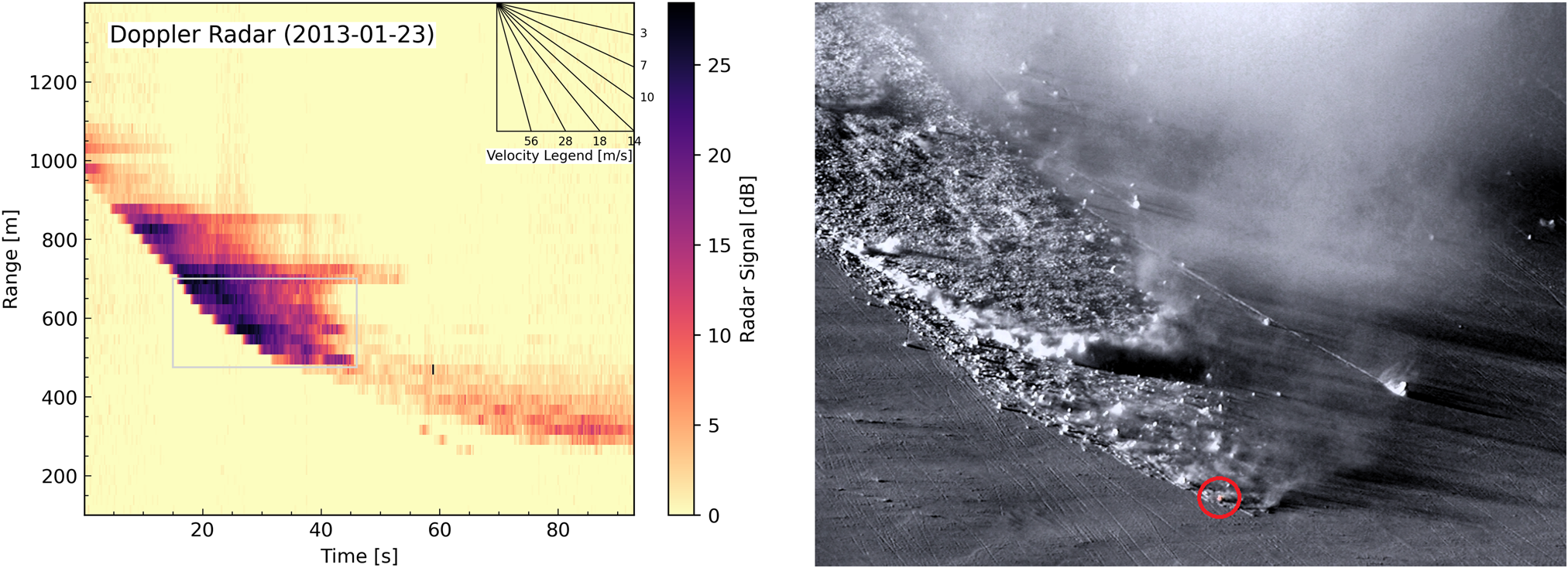
A qualitative analysis of the recorded IMU data allows to identify the main particle motion phases. The corresponding signals are depicted in Figures 4 and 5. The supplementary video serves as a visual reference.
Phase 0: Sensor unit at rest for time t < 0. Acceleration measurements correspond to the gravitational acceleration and allow (together with the magnetic field) to deduce the angular orientation of the sensor unit.
Phase 1: Entrainment at t = 0. The sensor unit is captured by the avalanche front and is heavily accelerated until t ≈ 0.6 s.
Phase 2: Ballistic motion. The sensor unit appears to be catapulted through the air. The measured acceleration signals are almost zero (i.e. inertial and gravitational forces nearly cancel each other) until t ≈ 1.4 s.
Phase 3: Impact. The sensor unit gets in contact with the dense snow again. Acceleration peak at t ≈ 1.4 s.
Phase 4: Steady flow. The sensor unit floats with the bulk of moving snow. The acceleration signal is dominated by random variations until t ≈ 15.5 s. Acceleration peaks indicate that some saltation (sequences of ballistic motion followed by impacts) takes place.
Phase 5: Rolling: The sensor unit leaves the avalanche at t ≈ 15.5 s and starts to roll downward. The fast-rolling character of the motion can be seen from high spin rates (exceeding the gyrometer measurement range) and from the oscillating behaviour of the magnetic field component (light green curves in Figs 4 and 5). The acceleration signals shift in the negative direction indicating a high centripetal acceleration due to high spin rates. At t ≈ 52 s the rotational motion starts to slow down continuously and stops at t ≈ 70 s.
Phase 6: Sensor unit at rest for $t\gtrsim 70$
 s
s

Top: Complete sequence of accelerometer (left) and gyrometer raw data (right) recorded in the course of the avalanche event (0 ≤ t ≤ 70 s). Bottom: Motion phases 0–4 (incomplete). As can be seen from the diagrams on the right-hand side, the gyrometers are saturated in a large part of the entire time span. To still be able to derive reliable information about the rotational motion, the local y component of the magnetic field is plotted in addition (light green curve).
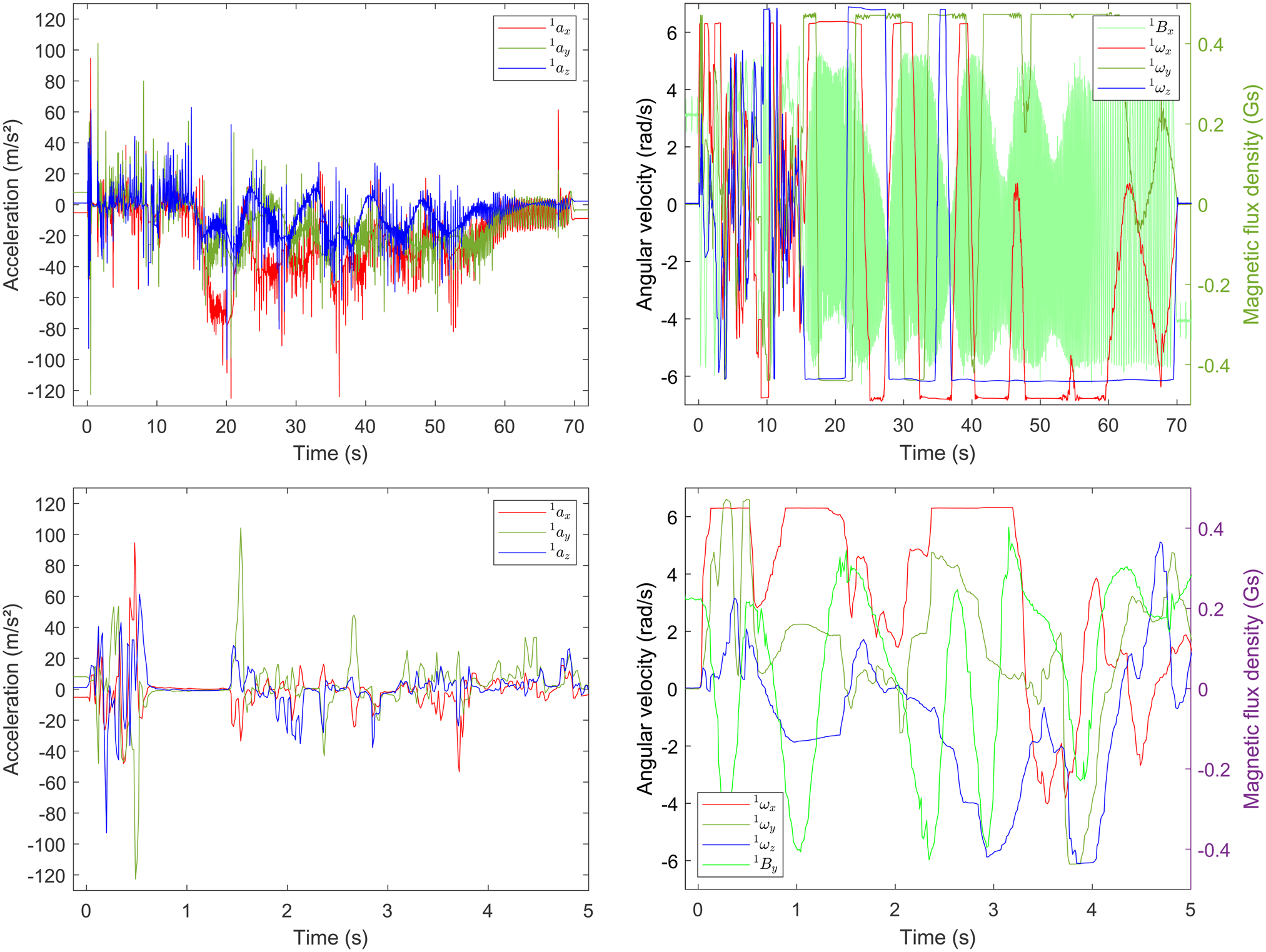
Top: Transition from motion phase 4 (steady flow) to phase 5 (rolling). Bottom: The final seconds of the rolling phase. The prominent acceleration peak (bottom-left) at t ≈ 67.7 s comes from an impact at the end of a small hill jump. The statement concerning the gyrometer data in the previous figure also applies here.

Particle motion phases 1–4 (entrainment, ballistic motion, impact, steady flow) are associated to the cold-dense flow regime, with particular emphasis on the initial rapid acceleration, which is associated with the corresponding avalanche velocities. The detachment of the main avalanche body at ≈15.5 s and subsequent transition to the snowball regime is represented by phase 5 (rolling) and followed by the final sensor unit deposition (phase 6).
4. Processing of inertial navigation data
4.1. Theory
In principle, IMUs are designed to enable the determination of angular orientation, translational velocity and position. While the reliability of angular orientation is usually high, the one of velocity and, even more, of position suffer from an unavoidable drift occurring in the course of an unavoidable integration procedure (Neurauter and Gerstmayr, Reference Neurauter and Gerstmayr2022). To obtain long-term stable results, additional information is required (GNSS data, e.g.). The Flüela experiment has revealed that the sensor unit in action has been subjected to high and strongly varying rotation rates (with a maximum of about 330 rpm ≈ 35 rad s−1 within the first 9 s) and to frequent and randomly distributed acceleration peaks, the strongest of which reaching almost 15 g (≈ 150 m s−2; see Figs 6 and 11). Considering the strongly, almost randomly, varying character of the raw data, it can be concluded that avalanche particle dynamics are dominated by stochastic rather than deterministic effects. These circumstances indicate that for the determination of velocity and position from the IMU data, standard methods of state estimation (see Crassidis and others, Reference Crassidis, Markley and Cheng2007, e.g.) are not well suited. These methods rely on the assumption that the state of a physical system is basically determined by a dynamical model and subjected to stochastic disturbances. While for simple types of motion (moving vehicles, e.g.), such models can be obtained from the trivial assumption of constant translational acceleration and constant angular velocity throughout each time interval, there is presently no concept from which an appropriate dynamical model could be derived for the translational and rotational motion of a particle driven by an avalanche. Therefore, an alternative procedure, subsequently called tracking algorithm for the evaluation of avalanche particle dynamics is proposed:
1. The angular orientation of the sensor unit is determined via an adapted integration procedure applied to the gyrometer and magnetometer data
2. At each time step, the corresponding rotation matrix is employed to transform the measured data from the local sensor frame to the global one
3. Velocity and position data are obtained from the global acceleration components via standard time integration (trapezoidal rule)
Left: Angular velocity components with respect to the corotating sensor coordinate system. Line colours red/dark green/blue refer to the measured values, magenta/green/cyan to the recovered ones. Right: Angular velocity components with respect to the global, inertial coordinate system.

4.1.1. Recovery of angular orientation
The tracking algorithm essentially relies on the knowledge of the angular orientation of the sensor system at every time step. The angular orientation at time t is uniquely determined by an orthogonal matrix

establishing an active rotation of the
inertial (global) coordinate axes
$( {\bf e}^0_x,\; \, {\bf e}^0_y,\; \, {\bf e}^0_z)$ onto the sensor-fixed (local)
coordinate frame (1ex,
1ey,
1ez), see
Figure 1. The kinematic
differential equation governing the evolution of
R(t) reads (Wittenburg, Reference Wittenburg2008)
onto the sensor-fixed (local)
coordinate frame (1ex,
1ey,
1ez), see
Figure 1. The kinematic
differential equation governing the evolution of
R(t) reads (Wittenburg, Reference Wittenburg2008)

with

being the skew-symmetric 3 × 3 matrix corresponding to the vector 0ω = [ 0ω x 0ω y 0ω z ]T of angular velocity components. To distinguish between vector components related to the corotating sensor frame and those related to the inertial frame, a left-hand superscript index is introduced, with 0 referring to the inertial and 1 to the corotating frame (compare Fig. 1). Inertial and corotating coordinates are related to each other via a passive rotation,

An efficient algorithm for the integration of (2) relies on the midpoint rule,

with Δt = t n+1 − t n being the time step size. The update scheme (5) ensures that the orthogonality of the rotation matrix is conserved.Footnote 6 An obvious choice for the mid-point angular velocities is given by

where 1ωn and 1ωn+1 are the measured, corotational angular velocity components at the n-th and (n + 1)-th time step, respectively. Equation (6) delivers an implicit definition of components 0ωn+1/2, which becomes apparent when inserting (5).
To derive additional advantage from the magnetometer data, the ansatz (6) is modified as follows. Use is made of the fact that the components of earth's magnetic field with respect to the global frame, 0B, are virtually constant in time,

In particular, Rn+1 1Bn+1 = 0B. It is important to have in mind that ||1B|| = ||0B|| = : B 0.
Inserting (5), a non-linear system of equations constraining the three components 0ωn+1/2 is obtained,

Note that the system (8) is
under-determined. Together with the three equations (6), an over-determined system
is obtained, from which the three components
${}^0{\boldsymbol \omega }^\ast _{n + {1}/{2}}$ can be determined via the least
squares method,Footnote 7
can be determined via the least
squares method,Footnote 7

Both systems, (6) and (8), have been scaled, such that they are free of any physical unit. In addition, a factor w n has been introduced, which allows to weight the two subsystems relatively to each other. This turns out to be beneficial, since the reliability of the measured magnetic field is not constant throughout the measurement period. The respective reliability can be estimated from the deviation of the norm ||1Bn|| from its expected value B 0. On the basis of numerical experiments the following weighting function has been established,

The parameter p is
determined such that the noise of the obtained global magnetic field
components is virtually the same for all three components
0B x,y,z(t),
see Figure 10, yielding a value of
p = 5. For each time step
n, the system (9) can be solved for the
ω* by means of the
Gauss–Newton method (Björck, Reference Björck1996). The rotation matrix is then updated via (5) with
${}^0{\boldsymbol \omega }_{n + {1\over 2}} = {\boldsymbol \omega }^\ast$ .
.
With the help of the updated rotation matrix Rn+1, the measured quantities 1Bn+1 (magnetic field), 1ωn+1 (angular velocity) and 1an+1 (acceleration) are transformed to the global coordinate system via a passive rotation,

To specify the initial orientation of the sensor unit, the global coordinate
system
$( {\bf e}^0_x,\; \, {\bf e}^0_y,\; \, {\bf e}^0_z)$ is defined according to the
geographic East-North-Up (ENU) convention: The global z and
y axes are upward vertical and geographic north,
respectively. At rest, the IMU measures an acceleration vector
1a0 = −1g,
with g being earth's gravitational acceleration vector
and a magnetic field 1B0, which is
considered to originate solely from earth's magnetism.
Correspondingly (Yun and others, Reference Yun, Bachmann and McGhee2008),
is defined according to the
geographic East-North-Up (ENU) convention: The global z and
y axes are upward vertical and geographic north,
respectively. At rest, the IMU measures an acceleration vector
1a0 = −1g,
with g being earth's gravitational acceleration vector
and a magnetic field 1B0, which is
considered to originate solely from earth's magnetism.
Correspondingly (Yun and others, Reference Yun, Bachmann and McGhee2008),

The vector components 1a0 and 1B0 have been determined by averaging the measured values over a time period of 0.2 s immediately before the sensor unit has been entrained by the avalanche. To be more precise, the declination D of earth's magnetic field has to be taken into account, such that

A value of
$D = 2.09705^\circ$ has been extracted according to
Schnegg (Reference Schnegg1998). Correspondingly,
the initial orientation is given by the rotation matrix
has been extracted according to
Schnegg (Reference Schnegg1998). Correspondingly,
the initial orientation is given by the rotation matrix

which is used to determine 0B = R0 1B0 and to initialize the integration procedure.
4.1.2. Recovery of translational velocity and position
It is essential to distinguish between the ‘kinematic’
acceleration vector, here denoted as
${}^0\dot {\bf v}_n$ , and the ‘dynamic’
acceleration vector 1an,
whose components are measured by the accelerometers. The former has to be
understood as negative inertial force vector per mass, and the latter as
guiding (or reaction) force per mass:Footnote 8 At rest, the kinematic acceleration is zero,
${}^0\dot {\bf v} = {\bf 0}$
, and the ‘dynamic’
acceleration vector 1an,
whose components are measured by the accelerometers. The former has to be
understood as negative inertial force vector per mass, and the latter as
guiding (or reaction) force per mass:Footnote 8 At rest, the kinematic acceleration is zero,
${}^0\dot {\bf v} = {\bf 0}$ , whereas an ideal accelerometer
triad is expected to measure the reaction to Earth's acceleration,
1a = −1g.
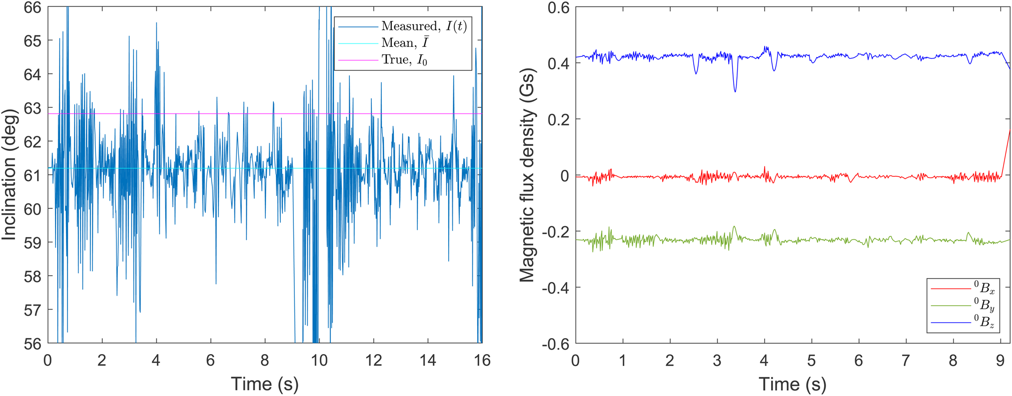
In the course of an ideal ballistic motion, the kinematic acceleration
equals Earth's acceleration,
${}^0\dot {\bf v} = {}^0{\bf g} = [ \, 0\; \; 0\; \; -g\, ] ^T$
, whereas an ideal accelerometer
triad is expected to measure the reaction to Earth's acceleration,
1a = −1g.
In the course of an ideal ballistic motion, the kinematic acceleration
equals Earth's acceleration,
${}^0\dot {\bf v} = {}^0{\bf g} = [ \, 0\; \; 0\; \; -g\, ] ^T$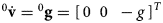 , whereas inertial forces and
earth's attraction cancel each other, such that
1a = 0.
Generally,
, whereas inertial forces and
earth's attraction cancel each other, such that
1a = 0.
Generally,

with

For a hypothetically perfect calibration of the accelerometers, one expects ||1a0|| to match the local value of Earth's gravitational acceleration (Schwartz and Lindau, Reference Schwartz and Lindau2003).
Equation (15) delivers the kinematic acceleration of the reference point, to which the measured accelerations are referred (see Fig. 1). The origin of the sensor coordinate system is arbitrarily chosen to be located at the geometric centre of the (almost) spherical housing. The respective coordinates of the reference point are

with an estimated accuracy of
±1 mm (Fig. 1). Taking
this eccentricity into account, the kinematic acceleration vector of the
centre point is obtained by compensating for the rotational inertia term,
$\dot {\boldsymbol \omega }\times {\boldsymbol \varepsilon }$ , and a centripetal acceleration,
${\boldsymbol \omega }\times ( {\boldsymbol \omega }\times {\boldsymbol \varepsilon })$
, and a centripetal acceleration,
${\boldsymbol \omega }\times ( {\boldsymbol \omega }\times {\boldsymbol \varepsilon })$ , see Wittenburg (Reference Wittenburg2008),

The angular acceleration
$\dot {\boldsymbol \omega }$ can be approximated by a
symmetric finite difference,
can be approximated by a
symmetric finite difference,

An estimate of sensor unit velocities is obtained by integrating the kinematic accelerations (18) via the trapezoidal rule with 0v0 = 0,

and, analogously, for the positions,

To understand the role of eccentricity and to quantitatively assess its
effect on velocity and position results, it is helpful to imagine what the
results of a hypothetically perfect tracking procedure (neither measurement
nor integration errors) are expected to be: such procedure would deliver the
trajectory of the centre point according to the translational motion
superimposed by the spiralling path of the accelerometer reference point
according to the rotational motion. Consequently, the trajectories of centre
and reference point, respectively, would not deviate from each other by more
than a distance of
$\Vert {}^1{\boldsymbol \varepsilon }\Vert$ . This gives rise to the
assumption, that also under realistic circumstances, the influence of a
small eccentricity on the trajectory is small, since the oscillating
disturbances related to the extra terms in (18) will largely be suppressed by the smoothing
effect of the numerical integration, as long as no parasitic aliasing occurs
related to the specific sampling rate. This assumption must, of course, be
verified on the basis of the experimental results, see the next section.
. This gives rise to the
assumption, that also under realistic circumstances, the influence of a
small eccentricity on the trajectory is small, since the oscillating
disturbances related to the extra terms in (18) will largely be suppressed by the smoothing
effect of the numerical integration, as long as no parasitic aliasing occurs
related to the specific sampling rate. This assumption must, of course, be
verified on the basis of the experimental results, see the next section.
4.2. Quantitative analysis based on standard calibration
Initially, the numerical analysis of the recorded IMU data has been applied to the time span [0, 16] s, which covers the period of avalanche motion. Correspondingly, the explications of this section refer to this time span, having in mind that the results for t > 9 s are corrupt. To not present misleading results, most diagrams are restricted to the time span [0, 9.2] s. The onset of data failure at t = 9.015 s can thus be observed at the very end of the drawn curves. Wherever a larger time span is presented, this is explicitly indicated and unreliable features are clearly identified by a dashed line style.
All results presented in this section refer to a calibration of accelerometers and gyrometers performed via conventional calibration procedures relying on laboratory experiments. Such procedures are state-of-the-art. The corresponding details are therefore postponed to Appendix A. The calibration of magnetometers is also performed by means of a state-of-the-art algorithm. The present approach, however, deviates from the standard procedure in one important aspect: to optimally account for the local conditions of Earth's magnetic field, the algorithm is supplied with magnetometer data recorded in the course of the avalanche experiment, i.e. with in situ data, rather than with laboratory data. Details can be found in Appendix A.
4.2.1. Slope coordinate system
It is a favourable circumstance that the relevant section of the terrain
which covers the first 9 s of the sensor unit motion is virtually
planar and can thus be approximated by an inclined plane with an inclination
of
$\alpha \approx 32^\circ$ . The projection of the vertical
axis
${\bf e}_z^0$
. The projection of the vertical
axis
${\bf e}_z^0$ onto this plane will be called
the slope secant. The name derives from the fact that it is
determined from the TLS terrain model and passes through the starting point
of the sensor unit and a corresponding point at the terrain surface in a
distance of 120 m, which is approximately the travelling distance
after 9 s. The (exactly straight) slope secant approximates the
(almost straight) slop line, which is the projection of the vertical axis
onto the actual terrain surface. Correspondingly, an additional Cartesian
coordinate frame
$( {\bf e}_x,\; \, {\bf e}^s_y,\; \, {\bf e}^s_z)$
onto this plane will be called
the slope secant. The name derives from the fact that it is
determined from the TLS terrain model and passes through the starting point
of the sensor unit and a corresponding point at the terrain surface in a
distance of 120 m, which is approximately the travelling distance
after 9 s. The (exactly straight) slope secant approximates the
(almost straight) slop line, which is the projection of the vertical axis
onto the actual terrain surface. Correspondingly, an additional Cartesian
coordinate frame
$( {\bf e}_x,\; \, {\bf e}^s_y,\; \, {\bf e}^s_z)$ , which is particularly useful for
the interpretation of the tracking results, can be defined in a
straight-forward manner: the first basis vector
${\bf e}^s_x$
, which is particularly useful for
the interpretation of the tracking results, can be defined in a
straight-forward manner: the first basis vector
${\bf e}^s_x$ is aligned with the slope secant.
The second basis vector
${\bf e}^s_y = {\bf e}_z^0\times {\bf e}^s_x$
is aligned with the slope secant.
The second basis vector
${\bf e}^s_y = {\bf e}_z^0\times {\bf e}^s_x$ is horizontal and tangent to the
corresponding contour line. The third one,
${\bf e}^s_z = {\bf e}^s_x\times {\bf e}^s_y$
is horizontal and tangent to the
corresponding contour line. The third one,
${\bf e}^s_z = {\bf e}^s_x\times {\bf e}^s_y$ represents the direction normal
to the terrain.Footnote 9 The so
defined basis will be called the slope coordinate system
(or frame) and its axis directions are referred to as
longitudinal
(${\bf e}^s_x$
represents the direction normal
to the terrain.Footnote 9 The so
defined basis will be called the slope coordinate system
(or frame) and its axis directions are referred to as
longitudinal
(${\bf e}^s_x$ ), lateral
(${\bf e}^s_y$
), lateral
(${\bf e}^s_y$ ) and transverse
(${\bf e}^s_z$
) and transverse
(${\bf e}^s_z$ ). The rotation tensor
transforming the inertial frame
$( {\bf e}_x^0,\; \, {\bf e}_y^0,\; \, {\bf e}_z^0)$
). The rotation tensor
transforming the inertial frame
$( {\bf e}_x^0,\; \, {\bf e}_y^0,\; \, {\bf e}_z^0)$ into the slope frame is given
by
into the slope frame is given
by

4.2.2. Rotational motion
The measurement range of the gyrometers, which has been chosen too small, has
lead to a cut-off of a few angular velocity peaks somewhat above
±6 rad s${^{-1}}$ (which is, in fact, larger than
the nominal range of
$\pm 300^\circ$
(which is, in fact, larger than
the nominal range of
$\pm 300^\circ$ s−1).
Luckily, whenever this has happened, not more than one out of the three
angular velocity components has been affected by saturation. Therefore, the
missing component can be recovered with the help of the magnetometer data.
The corresponding procedure is described in detail in Appendix B. The
results are shown in Figure 6
(left). The recovered curves provide a smooth continuation of the measured
ones.
s−1).
Luckily, whenever this has happened, not more than one out of the three
angular velocity components has been affected by saturation. Therefore, the
missing component can be recovered with the help of the magnetometer data.
The corresponding procedure is described in detail in Appendix B. The
results are shown in Figure 6
(left). The recovered curves provide a smooth continuation of the measured
ones.
An estimate Rn for the angular orientation of the sensor unit at any time step t n in the considered time interval is obtained by integrating the calibrated gyrometer data (Eqn (5)). For this purpose, the mid-point values of angular velocity components, 0ωn+1/2, are calculated by solving the overdetermined, non-linear equation system (9) via the Gauß–Newton method. The integration procedure is initialized with the starting orientation given by (14). It shall be mentioned here (and will be discussed subsequently), that the recovered angular orientation relies not only on angular rates, but also on magnetometer data and on accelerometer data (via the initial orientation). The rotational motion so obtained can be visualized and interpreted favourably via the evolution of the rotation (or Euler) vector φn, which is implicitly defined by

Wittenburg (Reference Wittenburg2008) with
Φn being the
skew-symmetric matrix composed from the components of vector
φn,
compare Eqn (3). The matrix
${\bf R}_n{\bf R}_0^T$ refers to the orientation at time
step t n relatively to the
initial orientation R0. It shall be noticed that the
components Rn and
φn
refer to the global, inertial coordinate system
$( {\bf e}_x^0,\; \, {\bf e}_y^0,\; \, {\bf e}_z^0)$
refers to the orientation at time
step t n relatively to the
initial orientation R0. It shall be noticed that the
components Rn and
φn
refer to the global, inertial coordinate system
$( {\bf e}_x^0,\; \, {\bf e}_y^0,\; \, {\bf e}_z^0)$ as well as to the local, moving
coordinate system
$( {\bf e}_x^1,\; \, {\bf e}_y^1,\; \, {\bf e}_z^1)$
as well as to the local, moving
coordinate system
$( {\bf e}_x^1,\; \, {\bf e}_y^1,\; \, {\bf e}_z^1)$ at the same time, i.e.
0Rn = 1Rn
and
0φn = 1φn
(Wittenburg, Reference Wittenburg2008).Footnote 10 For a straight-forward
interpretation of the rotational motion it is, however, beneficial to
express the rotation vector with respect to the slope frame
$( {\bf e}_x^s,\; \, {\bf e}_y^s,\; \, {\bf e}_z^s)$
at the same time, i.e.
0Rn = 1Rn
and
0φn = 1φn
(Wittenburg, Reference Wittenburg2008).Footnote 10 For a straight-forward
interpretation of the rotational motion it is, however, beneficial to
express the rotation vector with respect to the slope frame
$( {\bf e}_x^s,\; \, {\bf e}_y^s,\; \, {\bf e}_z^s)$ , indicated through the left
superscript symbol ‘s’,
, indicated through the left
superscript symbol ‘s’,

The result is drawn in Figure 7 and compared to the angular
velocity components
${}^s{\boldsymbol \omega }_n = {\bf Q}_s^T{}^0{\boldsymbol \omega }_n$ with respect to the same frame.
It can be concluded from these diagrams that in the course of the first
3.2 s the rotational motion is dominated by a fast rotation about the
horizontal
${\bf e}^s_y$
with respect to the same frame.
It can be concluded from these diagrams that in the course of the first
3.2 s the rotational motion is dominated by a fast rotation about the
horizontal
${\bf e}^s_y$ -axis at an average speed of
$7.81\, {\rm rad}\, {\rm s} {^{-1}}\approx 477^\circ \, {\rm s}\, {^{-1}}\approx 1.24$
-axis at an average speed of
$7.81\, {\rm rad}\, {\rm s} {^{-1}}\approx 477^\circ \, {\rm s}\, {^{-1}}\approx 1.24$ rounds per second. In this time
period, the sensor unit performs a number of four full twits about the
${\bf e}^s_y$
rounds per second. In this time
period, the sensor unit performs a number of four full twits about the
${\bf e}^s_y$ -axis. The first twist is the
fastest one with an average speed of
$12.36\, {\rm rad}\, s {^{-1}}\approx 708^\circ \, {\rm s} {^{-1}}\approx 1.97$
-axis. The first twist is the
fastest one with an average speed of
$12.36\, {\rm rad}\, s {^{-1}}\approx 708^\circ \, {\rm s} {^{-1}}\approx 1.97$ rounds per second and an
instantaneous velocity peak of approximately
$35\, {\rm rad}\, {\rm s} {^{-1}}\approx 2000^\circ \, {\rm s} {^{-1}}\approx 5.5$
rounds per second and an
instantaneous velocity peak of approximately
$35\, {\rm rad}\, {\rm s} {^{-1}}\approx 2000^\circ \, {\rm s} {^{-1}}\approx 5.5$ rounds per second.Footnote 11 For
t > 3.2 s, the rotational
motion continues at a lower speed and without a stable rotation axis. As
mentioned before, the results for
t > 9 s are corrupt due to a
data gap and are, thus, not displayed here. A demonstrative visualization of
the rotational motion is presented in Figure 8. For the visualization, the path
r(t) drawn there is the trajectory of a
point on a hypothetical sphere with an (arbitrarily chosen) radius of
r = 5 m which is thought to
move and rotate in the same way as the sensor unit does,
i.e.
rounds per second.Footnote 11 For
t > 3.2 s, the rotational
motion continues at a lower speed and without a stable rotation axis. As
mentioned before, the results for
t > 9 s are corrupt due to a
data gap and are, thus, not displayed here. A demonstrative visualization of
the rotational motion is presented in Figure 8. For the visualization, the path
r(t) drawn there is the trajectory of a
point on a hypothetical sphere with an (arbitrarily chosen) radius of
r = 5 m which is thought to
move and rotate in the same way as the sensor unit does,
i.e.

Rotation vector (left) and angular velocity (right) components with respect to the slope frame.

Red: Trajectory of the centre of the sensor housing, x(t), corresponding to the time interval [0, 9] s. Blue: Trajectory of a hypothetical tracing point in a constant distance of 5 m from the centre, r(t), for visualization of the rotational motion. Left: Axonometric view. Right: Top view, i.e. a normal projection of the trajectory onto a horizontal plane.
4.2.3. Magnetic field
It has been described in detail how the magnetometer data can be used to stabilize the integration of angular rates (Section 4.1.1) and to bridge short gaps with deficient gyrometer data (Appendix B). In addition, the measured magnetic flux density can give an evidence to assess the reliability of the recovered angular orientations. In this context, a proper calibration is crucial. At the absence of ferromagnetic disturbances it can be assumed that the vector of the magnetic flux density, and thus its components with respect to the inertial frame, 0B, are virtually constant in space and time. Consequently, the norm of the local components ||1B|| is expected to be constant as well,

A sufficiently accurate fulfilment of Eqn (25) is thus a necessary condition for the measured values and, in particular, for the calibration to be reliable. A significant deviation from the expected value is used to define a quantitative reliability measure according to Eqn (10), which governs the effect of the magnetometer data on the angular orientations, compare Figure 9.
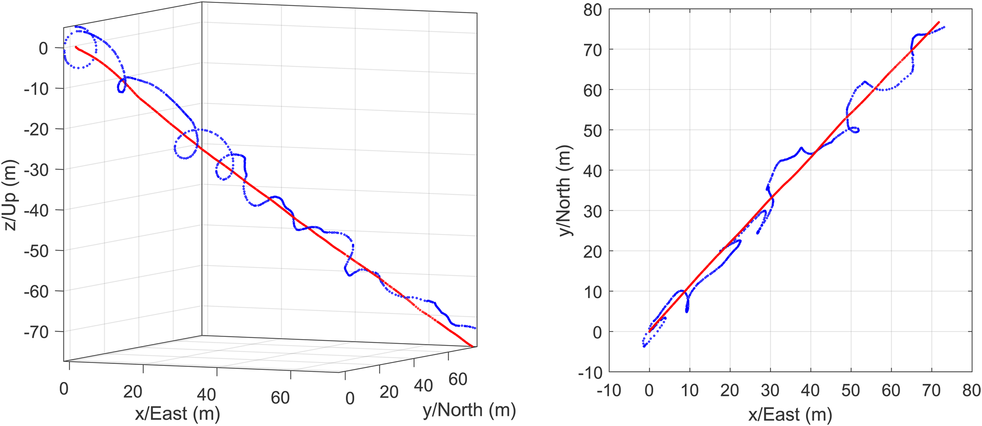
Left: Vector norm of the local components of the magnetic flux density, ‖1B‖, subjected to a calibration under laboratory conditions carried out some time after the avalanche experiment (cyan) and to an in situ calibration according to Appendix B (blue). The reliability measure (gray) is calculated from (10). Right: Local components of the magnetic flux density, 1Bk, subjected to in situ calibration.

Left: Inclination
I(t n)
calculated from
0B(t n)
via Eqn (27b),
its mean value
$\bar I$ and the true value
I 0. Right:
Global components of the magnetic flux density,
0B x,y,z.
The B components involved are subjected to in
situ calibration, whereas the initial orientation relies on
accelerometer data subjected to laboratory
calibration.
and the true value
I 0. Right:
Global components of the magnetic flux density,
0B x,y,z.
The B components involved are subjected to in
situ calibration, whereas the initial orientation relies on
accelerometer data subjected to laboratory
calibration.
A necessary condition for the reliability of the recovered orientations R(t) is given by the constancy of the global components of B,

which is illustrated in Figure 10. It is also worth to discuss
the direction of vector B specified via spherical (azimuthal
and polar) angles, φ and
$\vartheta$ . Defining these angles with
respect to the global ENU coordinate system
$( {\bf e}^0_x,\; \, {\bf e}^0_y,\; \, {\bf e}^0_z)$
. Defining these angles with
respect to the global ENU coordinate system
$( {\bf e}^0_x,\; \, {\bf e}^0_y,\; \, {\bf e}^0_z)$ , one has

with declination D and inclination I.
According to Schnegg (Reference Schnegg1998), at the
time and location of the experiment, the corresponding values are
$D_0 = 2.09705^\circ$ and
$I_0 = 62.81433^\circ$
and
$I_0 = 62.81433^\circ$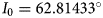 . The declination has already been
used for the specification of the starting orientation in (13) and can therefore
not serve for any further verification. The
inclination, on the other hand, has not been considered so far. Calculating
the latter from the global magnetic field components via Eqn (27b), values are obtained
which oscillate around a mean value of
$\bar I \approx 61.19^\circ$
. The declination has already been
used for the specification of the starting orientation in (13) and can therefore
not serve for any further verification. The
inclination, on the other hand, has not been considered so far. Calculating
the latter from the global magnetic field components via Eqn (27b), values are obtained
which oscillate around a mean value of
$\bar I \approx 61.19^\circ$ with a standard deviation of
$1.3^\circ$
with a standard deviation of
$1.3^\circ$ (see Fig. 10). Thus, a deviation of
$I_0-\bar I\approx 1.62^\circ$
(see Fig. 10). Thus, a deviation of
$I_0-\bar I\approx 1.62^\circ$ from the expected value
I 0 is observed. This result reveals a
moderate error in the recovered orientations.
from the expected value
I 0 is observed. This result reveals a
moderate error in the recovered orientations.
4.2.4. Translational motion
In Figure 11, at the left-hand side,
the dynamic acceleration components with respect to the sensor frame,
1a, are drawn. These are the values measured by
the accelerometers and subjected to laboratory calibration. At the
right-hand side, the kinematic acceleration components with respect to the
inertial frame,
${}^0\dot {\bf v}$ , Eqn (18), are plotted. It is
emphasized that, in contrast to the 1a, the
${}^0\dot {\bf v}$
, Eqn (18), are plotted. It is
emphasized that, in contrast to the 1a, the
${}^0\dot {\bf v}$ rely on the whole set of
measurement data, since the rotation matrix R is required for
the coordinate transformation (11).
rely on the whole set of
measurement data, since the rotation matrix R is required for
the coordinate transformation (11).
Left: Dynamic acceleration components with respect to the local coordinate system. Right: Kinematic acceleration components with respect to the global coordinate system.
The clear representation of ballistic motion is considered as a certain
evidence for the reliability of the measurements: a pronounced ballistic
phase starts at t ≈ 0.85 s and
is followed by several shorter ones, especially in the time period from
t ≈ 7.6 s to
t ≈ 9 s, during which a
sort of saltational motion occurs (short ballistic phases interrupted by
impacts; see Fig. 12). The ballistic
phases are represented by the expected values of
${}^0\dot {\bf v} = [ 0\; 0\; -g] ^T$ .
.
Kinematic acceleration components related to the global frame: selected time intervals dominated by ballistic or saltational motion.

Knowing the evolution of the kinematic acceleration, the sensor unit trajectory can be recovered according to Section 4.1.2. Projections of the obtained trajectory and of the reference tube (Section 2) are depicted in Figure 13. The plots refer to the whole time span [0, 16] s in order to demonstrate the parasitic effect of the data gap at t ≈ 9 s. Correspondingly, the second third of the path (dashed lines) might be dismissed. Note that the reference domain applying to the top view (left diagram) is also drawn in Figure 2 and recall that the reference domain for the vertical section (right diagram) is aligned with the terrain surface (including the snow cover) and has an assumed vertical span of ±1 m.
Sensor unit trajectory recovered from IMU data according to Section 4.1.2 and compared to the reference defined in Section 1. The heavy deviations from the reference in the second third of the path (dashed lines) are a result of the data gap at t ≈ 9 s and might be dismissed. Left: Top view, i.e. a normal projection onto a horizontal plane. The blue and red curves refer to an evaluation of (18) with and without consideration of eccentricity, respectively. Right: Vertical section, i.e. a normal projection onto a vertical plane passing through the slope line.

Figure 13 also demonstrates the
influence of the eccentricity
${}^1{\boldsymbol \varepsilon }$ included in Eqn (18): the blue and red curves
refer to an evaluation of (18) with and without consideration of eccentricity, i.e. with
${}^1{\boldsymbol \varepsilon }$
included in Eqn (18): the blue and red curves
refer to an evaluation of (18) with and without consideration of eccentricity, i.e. with
${}^1{\boldsymbol \varepsilon }$ given by (17) and with
${}^1{\boldsymbol \varepsilon } = {\bf 0}$
given by (17) and with
${}^1{\boldsymbol \varepsilon } = {\bf 0}$ , respectively. The small extend
of the deviation of the corresponding results indicates that the
considerations of Section 4.1.2
concerning the effect of eccentricity are applicable. In particular, the
sensitivity of the tracking results to a small change of the eccentricity
vector is negligible. Accordingly, an eccentricity given by (17) is considered for all
subsequent computations.
, respectively. The small extend
of the deviation of the corresponding results indicates that the
considerations of Section 4.1.2
concerning the effect of eccentricity are applicable. In particular, the
sensitivity of the tracking results to a small change of the eccentricity
vector is negligible. Accordingly, an eccentricity given by (17) is considered for all
subsequent computations.
A comparison of the recovered trajectory with the reference reveals a
somewhat unexpected behaviour: referring to the top view in Figure 13 (left), the numerical result
matches the reference surprisingly well. A slight but progressive lateral
movement is observed. The most likely explanation for this behaviour is a
(quadratic) numerical drift, which is expected due to the twofold
integration procedure leading to the position results. However, it cannot be
excluded, that (to a small extent) the lateral movement also reflects a
physical motion. In contrast, the vertical section in Figure 13 (right) reveals a significant deviation
from the terrain surface, which is physically impossible. This deviation is
more like an overall misalignment rather than an expected drift, since it is
present even at the beginning of the movement and is virtually constant
throughout the path (until the data gap occurs at
t ≈ 9 s). This observation is
supported by the dotted red line in the right diagram, which results from a
rotation of the solid red line by an assumed angle of
$6^\circ$ in the vertical section
plane.
in the vertical section
plane.
5. Accelerometer in situ calibration
5.1. Theory
In this section, a theory is presented, which provides an explanation for the misalignment of the recovered trajectory, addressed at the end of the previous section. In addition, the underlying assumption leads to a novel procedure to eliminate the misalignment error, for which the term ‘in situ calibration’ is suggested.
If the misalignment would originate from stochastic errors, its magnitude should be small at the beginning and should increase more or less monotonically afterwards, which is not the case. Consequently, it can be concluded that the source of error is of systematic nature. At a first glance, a wrong initial orientation R0 would deliver an obvious explanation for the misalignment. This possibility, however, can be excluded by the verification of the orientation results presented in Section 4.2.3. Instead, it is postulated that the observed deviation originates from an inaccurate calibration of accelerometers. This assumption appears realistic, since the original calibration procedure (Appendix A) has been carried out under laboratory conditions 5 years after the avalanche experiment. Subsequently, it will be explicated, how a recalibration can be obtained on the basis of the data recorded in the course of the avalanche event, i.e. on the basis of in situ data. Recall that a related approach for the recalibration of magnetometers has been addressed in Section 4.2.3. Although these two fields of application (accelerometers and magnetometers) require two fundamentally different procedures, they have one important aspect in common: the reliability of the recalibration procedures essentially relies on the characteristics of the rotational motion. To start with, this shall be demonstrated for the case of magnetometer recalibration: mathematically speaking, the subset of orientations Rn occurring in the course of the motion must be evenly distributed in the set of all possible orientations; or, less abstract, the tips of normalized vectors 1Bn/||1Bn|| must be evenly distributed on the unit sphere. The more bias occurs among this distribution (i.e. the less complex the rotational motion is), the worse is the conditioning of the equation system determining the calibration parameters and thus, the lower is the reliability of its solution (Appendix A). Although less obvious, an analogous statement holds for the accelerometer recalibration. In the present case, the orientations are spread over the whole sphere but are far from being uniformly distributed (Fig. 21). It turns out, however, that such a degree of uniformity is sufficient to achieve valuable results.
5.1.1. Accelerometer error model
The recalibration of the three-axis accelerometer based on in situ data
relies on a common, linear error model, similar to the one which has already
been used for the standard calibration procedure (Appendix A): it is assumed
that the ‘true’ acceleration values
1an are related
to the measured ones,
${}^1\tilde {\bf a}_n$ , via
, via

Here, the calibration matrix A = I + C is assumed to deviate only slightly from the identity matrix I. It allows for scaling errors, non-orthogonality and misalignment of the physical sensor axes relatively to the axes of the sensor coordinate system. The additive offset consists of a constant part (bias) g b0 and a linear drift g b1. Earth's acceleration g has been premultiplied to achieve calibration parameters which are independent of the choice of physical units. Due to the same reason, a dimensionless time parameter is used,

with N being the index of the last considered time step. The recalibration also affects 0g (Eqn (16)), which becomes

For the proposed implementation, the ‘true’ values are adopted, i.e. 0g = [ 0 0 − g ]T with g = 9.802 m/s−2 for the local region.Footnote 12 The kinematic acceleration vectors (Eqn (15)) now read

By rearranging the calibration parameters

the vectors

are obtained, by which means Eqn (31) can be given a concise shape,

Therein,

are the kinematic acceleration vectors ahead of recalibration. The (3 × 6)-matrices

impart the correction according to bias and drift, whereas the (3 × 9)-matrices

are related to the correction of scaling, non-orthogonality and misalignment. They are composed of columns

where
${\bf R}^{( n) }_{\, \colon \, , i}$ denotes the i-th
column of the rotation matrix Rn
and
${}^1\tilde a^{( n) }_j$
denotes the i-th
column of the rotation matrix Rn
and
${}^1\tilde a^{( n) }_j$ the j-th
component of vector
${}^1\tilde {\bf a}_n$
the j-th
component of vector
${}^1\tilde {\bf a}_n$ .
.
The improved kinematic accelerations (34) yield improved velocity and position vectors,


Again,
${}^0\tilde {\bf v}_n$ and
${}^0\tilde {\bf x}_n$
and
${}^0\tilde {\bf x}_n$ denote the results ahead of
recalibration, and
denote the results ahead of
recalibration, and


The integration is again performed via the trapezoidal rule. Correspondingly, the integral operations in Eqns (39)–(42) have to be understood as

5.1.2. Topography constraint
In fact, the sensor unit has moved close to the topographic surface (terrain). Consequently, the recovered trajectory is also supposed to develop close to this surface. This gives rise to postulate a soft constraint either at the velocity level,

or at the position level,

with k being the vector
normal to the topographic surface. Equations (44) and (45) claim that the component normal to the terrain either of the
velocity or of the relative position is minimum in a least squares sense. To
formulate these constraint conditions, the surface normal vector
k is required, which can, in principle, be obtained from
the TLS data. In the present case, k is almost constant and can
be approximated by
${\bf k} = {\bf e}^s_z$ (Section 4.2.1). This circumstance makes the implementation
significantly easier. It is, however, not a mandatory
requirement for the method to work properly. Inserting (39) and (40), the constraint
conditions (44) and (45) become
(Section 4.2.1). This circumstance makes the implementation
significantly easier. It is, however, not a mandatory
requirement for the method to work properly. Inserting (39) and (40), the constraint
conditions (44) and (45) become


Conditions (46) and (47) are equivalent to the overdetermined systems of equations,

respectively. For conciseness, the following (N × 1)-vectors,


as well as (N × 6)- and (N × 9)-matrices,

have been introduced. Each of Eqns (48a) and (48b) constitutes an overdetermined, linear system of N equations for the 6 + 9 = 15 unknowns contained in vectors b and c. As discussed at the beginning of Section 5, the rotational motion involved must display a certain degree of complexity, to ensure that matrices (51a) and (51b) have full rank (i.e. 6 and 9, respectively). Consequently, each of the two equation systems yields a unique solution, which will be denoted (bx, cx) for the position level constraint and (bv, cv) for the velocity level.
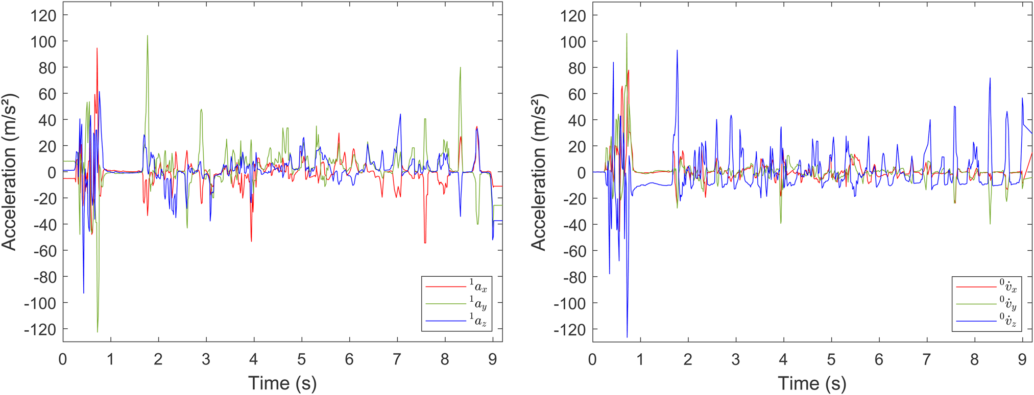
5.1.3. Regularization
Determining the calibration parameters is a sort of inverse problem. In fact, none of the solutions of systems (48) is feasible, since at least some of the calibration parameters obtained (their absolute values) are too large, i.e. in the order of 1. This contrasts the original intention to search for a small correction of pre-calibrated values. Accordingly, the minimization problem has to be reformulated to search for a compromise between minimizing the overall deviation from the topographic surface and minimizing the calibration parameters. To this end, the objective functions are enriched by regularization terms,


This approach is well known as Tychonov regularization (Strang, Reference Strang2007). The scalings involving Earth's acceleration g and the span T of the considered time interval have been introduced to provide the respective regularization term with the correct physical unit. The optimal choice for the regularization parameter is ρ = 1, which will be verified in the next section (compare Fig. 14): firstly, the smallest minimum of the objective function can be achieved for this choice. Secondly, the minimum is relatively insensitive to a variation of the parameter in a certain interval around 1 (see Fig. 14). Again, the minimization problem (52) is equivalent to an overdetermined system, namely to the system of N + 6 + 9 equations,

and analogously for (53),

Therein, I6 is the (6 × 6)-identity matrix, O9×6 the (9 × 6)-zero matrix, 06 = O6×1, etc.
Left: Local acceleration components before (red/dark green/blue) and after (magenta/green/cyan) recalibration. Right: Obtained minima of the objective functions according to the minimization problems (52) and (53), respectively, in dependence of the regularization parameter ρ. Note that the minimum objective function can be considered as a measure for the violation of the constraint condition.
5.2. Quantitative analysis based on in situ calibration
5.2.1. Determination of calibration parameters
The parameter vectors b and c of the accelerometer
error model result from the postulate that the constraint condition is
fulfilled in a least squares sense either at position level or at velocity
level (Eqns (44) and (45), respectively). To this
end, the overdetermined systems of equation (54) or (55) have to be solved. The input quantities entering this
procedure are: Rn,
${}^1\tilde {\bf a}_n$ ,
${}^0\tilde {\bf v}_n$
,
${}^0\tilde {\bf v}_n$ and
${}^0\tilde {\bf x}_n$
and
${}^0\tilde {\bf x}_n$ . The tilde refers to values based
on the laboratory calibration (prior to recalibration).
. The tilde refers to values based
on the laboratory calibration (prior to recalibration).
Applying the velocity constraint without considering the linear drift term involving b1, one obtains

whereas the position constraint yields

From a physical point of view, the two constraint conditions are expected to yield similar results. In fact, the values of corresponding parameters differ by less that ±20%,

with the relative difference being
defined as
$\delta {\bf b} = ( {\bf b}_0^{( v) }-{\bf b}_0^{( x) }) /( \Vert {\bf b}_0^{( v) }\Vert + \Vert {\bf b}_0^{( x) }\Vert )$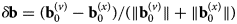 and analogously for
δ c. On a first glance, the impact
of the recalibration on the acceleration components is small (see Fig. 14, left). Its impact on the
recovered trajectories, however, is significant, as will be explicated in
detail in the next section. The recalibration also effects the determination
of the initial orientation R0 (Eqns (12)–(14)). This effect can be
quantified by identifying the rotation vector
δ φ(x)
related to the rotation matrix
$\delta {\bf R} = {\bf R}_{0, recal}{\bf R}_0^T$
and analogously for
δ c. On a first glance, the impact
of the recalibration on the acceleration components is small (see Fig. 14, left). Its impact on the
recovered trajectories, however, is significant, as will be explicated in
detail in the next section. The recalibration also effects the determination
of the initial orientation R0 (Eqns (12)–(14)). This effect can be
quantified by identifying the rotation vector
δ φ(x)
related to the rotation matrix
$\delta {\bf R} = {\bf R}_{0, recal}{\bf R}_0^T$ ,
,

Thus, the observed inclination of the magnetic field changes according to

That is, the correction of the
inclination tends in the right direction, though it is too large, such that
$I_0 - I_x\approx -1.10^\circ$ (instead of
$+ 1.62^\circ$
(instead of
$+ 1.62^\circ$ prior to recalibration). Now the
absolute error goes below the standard deviation
($1.3^\circ$
prior to recalibration). Now the
absolute error goes below the standard deviation
($1.3^\circ$ ). The given numbers refer to the
position constraint. For the velocity constraint, the angular deviation is
even more
pronounced,
). The given numbers refer to the
position constraint. For the velocity constraint, the angular deviation is
even more
pronounced,

such that the error of the observed
inclination becomes
$I_0 - I_v\approx -1.89^\circ$ , which is even (absolutely)
larger than the error prior to recalibration.
, which is even (absolutely)
larger than the error prior to recalibration.
Concluding, the influence of the regularization parameter
ρ entering the minimization problems (52) and (53), respectively, shall be
investigated (see Fig. 14, right).
For the velocity as well as for the position constraint, the smallest
minimum of the objective function is achieved for
ρ = 1. Moreover, the minimum is
relatively insensitive to a variation of the parameter in a certain interval
around 1. There is a pronounced interval of insensitivity for the position
constraint
($5\cdot 10^{-2}\lesssim \rho \lesssim 5$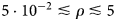 ). This is a necessary condition
for the regularization approach to be valid. For the velocity constraint,
this interval is significantly smaller, which makes the corresponding
results less robust. Note that the sensitivities of the minimum objective
function with respect to a variation of the regularization parameter are
scalar measures for the sensitivities of the position and velocity
functions, x(t) and
v(t), respectively. Referring to the
interval
5 ⋅ 10−2 ≤ ρ ≤ 5,
the variation of the minimum objective function is in the range of
±0.02. Correspondingly, the variation of the
x(t) function is of the same order of
magnitude
($\sim \pm 2\%$
). This is a necessary condition
for the regularization approach to be valid. For the velocity constraint,
this interval is significantly smaller, which makes the corresponding
results less robust. Note that the sensitivities of the minimum objective
function with respect to a variation of the regularization parameter are
scalar measures for the sensitivities of the position and velocity
functions, x(t) and
v(t), respectively. Referring to the
interval
5 ⋅ 10−2 ≤ ρ ≤ 5,
the variation of the minimum objective function is in the range of
±0.02. Correspondingly, the variation of the
x(t) function is of the same order of
magnitude
($\sim \pm 2\%$ ).
).
5.2.2. Constrained trajectory
The calibration parameters obtained from the two different types of constraint conditions (and an accelerometer error model (28) involving a constant bias but no drift) are subsequently used to recalibrate the accelerometer values, which, in turn, are applied to calculate new estimates of the sensor unit trajectory. In Figure 15, these results are compared to each other, to the original estimate of the trajectory according to standard calibration on the basis of laboratory data, and to the reference tube. According to the design of the method, the vertical projections of the constrained trajectories (right diagram in the figure) match the terrain line in an averaged sense. In contrast, dealing with the vertical projection (left diagram), the overall deviation of the constrained trajectories from the reference tube appears to become larger compared to their unconstrained counterpart. For a more detailed assessment of the new results it is beneficial to consider the position coordinates with respect to the slope coordinate system,

That is, sx (longitudinal coordinate) is the distance from the starting point of the sensor unit measured along the slope secant (Section 4.2.1); sy (lateral coordinate) and sz (transverse coordinate) are the normal distances from the slope secant measured in horizontal direction and in the slope normal direction, respectively. With other words, sx is approximately the travelling distance, sy and sz measure the deviation from the slope secant. Accordingly, Figure 16 shows the deviation of the estimated trajectories from the slope secant. The following conclusions can be drawn from the diagrams:
1. The acceleration phase ranging from sx = 0 m to sx ≈ 1 m is accompanied by a small lateral movement in the order of 0.1 m.
2. The ballistic motion phase at the beginning of the sensor unit movement is clearly represented in the trajectory plot, where it appears in the shape of a ballistic parabola ranging from sx ≈ 1 m to sx ≈ 21 m (right diagram in Fig. 16).
3. The reliability of the unconstrained trajectory is poor, since the orientation of the ballistic parabola is not plausible. (A correct starting orientation of the trajectory is considered as a necessary condition for the reliability of a tracking procedure.)
4. The starting orientations of the constraint trajectories are within an acceptable range.
5. Each of the trajectories constrained in transverse direction suffers from a severe (basically quadratic) drift in the lateral direction (left diagram), which is to be expected, given the low sampling rate applied (compared to contemporary standards).
6. The transverse deviation from the slope line (right diagram) is of the same order of magnitude as the estimated accuracy of the reference tube until it starts to diverge close to the end of the processed time interval (corresponding to a travelling distance of ≈120 m).Footnote 13
7. Based on the trajectory results, a clear preference for the position or the velocity constraint cannot be deduced. The explications of the previous section, however, assign a higher reliability to the position constraint.
Sensor unit trajectories recovered from IMU data subjected to laboratory calibration (red) and to in situ calibration based on velocity (cyan) and position constraint (blue), respectively. The projections of the reference tube are shown in grey. Left: Top view, i.e. a normal projection onto a horizontal plane. Right: Vertical section, i.e. a normal projection onto a vertical plane passing through the slope secant.

Estimates of the sensor unit trajectory drawn in the inclined x-y plane (i.e. approximately the terrain surface) of the slope coordinate system (left) and in the vertical x-z plane (right). The vertical grey lines indicates the end of the ballistic flight path. The horizontal lines passing through the origin refer to the slope secant. Correspondingly, the left and right diagrams show the lateral and transverse deviation from the slope secant. Note that the reference tube is derived from the measured terrain model and is therefore not aligned exactly with the slope secant.

The calculations have been repeated, once without considering any bias, i.e. b0 = b0 = 0 and once with all terms included in the error model (28), i.e. considering constant bias and linear drift and are referred to as
1. No bias: ${}^1{\bf a}_n = ( {\bf I} + {\bf C} ) {}^1\tilde {\bf a}_n$
2. Constant bias: ${}^1{\bf a}_n = ( {\bf I} + {\bf C} ) {}^1\tilde {\bf a}_n + g{\bf b}_0$
3. Linear drift: ${}^1{\bf a}_n = ( {\bf I} + {\bf C} ) {}^1\tilde {\bf a}_n + g{\bf b}_0 + g\tau _n{\bf b}_1$
The corresponding tracking results are summarized in Figure 17. It turns out that models (2) and (3) yield virtually identical results, whereas model (1) does not work properly. This observation holds for the velocity as well as for the position constraint. Clearly, approach (2) is to be preferred since approach (3) relies on a larger number of parameters without delivering better results. Thus, all position and velocity results presented in this section without an explicit reference to the error model rely on approach (2).
Comparison of error models (1)–(3) for the velocity (top) and position constraint (bottom).

5.2.3. Translational velocities
The recovered translational velocity components are plotted in Figure 18. In the left diagram, the
global components obtained before (cyan, green, magenta refer to global
z, x, y components,
respectively) and after recalibration (red, darkgreen, blue) are compared to
each other. Apparently, the vertical velocity component
0v z is effected
most by the recalibration. This is what has to be expected according to the
nature of the constraint condition. The divergence of the results according
to position and velocity constraints is less significant (solid vs. dotted
lines). There is also a certain deviation in the evolution of the
0v y components,
which reflects the drift observed in the horizontal projection of the
trajectory and is thus considered as a result of accumulated noise with no
physical significance. For a further interpretation of the velocity results
it is again useful to consider the components with respect to the slope
coordinate system (Section 4.2.1), i.e.
${}^s{\bf v} = {\bf Q}_s^T{}^0{\bf v}$ , which are plotted in the right
diagram of Figure 18.
Correspondingly,
sv x
refers to the direction of the slope secant (longitudinal),
sv y,
to the horizontal (lateral) direction and
0v z to the
direction normal to the terrain (transverse). As expected, the
sv y
values are relatively small. However, instead of simply oscillating around
zero, they reveal the linear drift mentioned before. The motion phases
identified within the qualitative IMU data analysis are reflected by the
velocity evolution:
, which are plotted in the right
diagram of Figure 18.
Correspondingly,
sv x
refers to the direction of the slope secant (longitudinal),
sv y,
to the horizontal (lateral) direction and
0v z to the
direction normal to the terrain (transverse). As expected, the
sv y
values are relatively small. However, instead of simply oscillating around
zero, they reveal the linear drift mentioned before. The motion phases
identified within the qualitative IMU data analysis are reflected by the
velocity evolution:
1. Acceleration phase from t ≈ 0.25 s to t ≈ 0.80 s: a strong and progressive increase of the sv x component occurs (Fig. 18, right).
2. Ballistic motion from t ≈ 0.80 s to t ≈ 1.67 s: horizontal components 0v x and 0v y are basically constant, while the vertical component −0v z is linearly increasing according to Earth's acceleration (Fig. 18, left). The evolution of the transverse component sv z indicates that a pronounced motion normal to the terrain surface occurs that changes from outward (sv z > 0) to inward (sv z < 0) orientation (Fig. 18, right).
3. Impact at t = 1.67 s: a sudden deceleration occurs in longitudinal (${\bf e}^s_x$
) as well as in
transverse direction
(${\bf e}^s_z$), see the right
diagram of Figure
18.4. ‘Steady flow’ motion starting at t ≥ 1.67 s: the motion is dominated by the longitudinal component sv x. It is slowly decelerating and is superimposed by a basically random jerking (Fig. 18, right).


Translational velocity components vs. time. Global components (left) and components with respect to the slope frame (right). Comparison of results before and after recalibration. Solid lines refer to the position constraint, dotted lines to the velocity constraint.
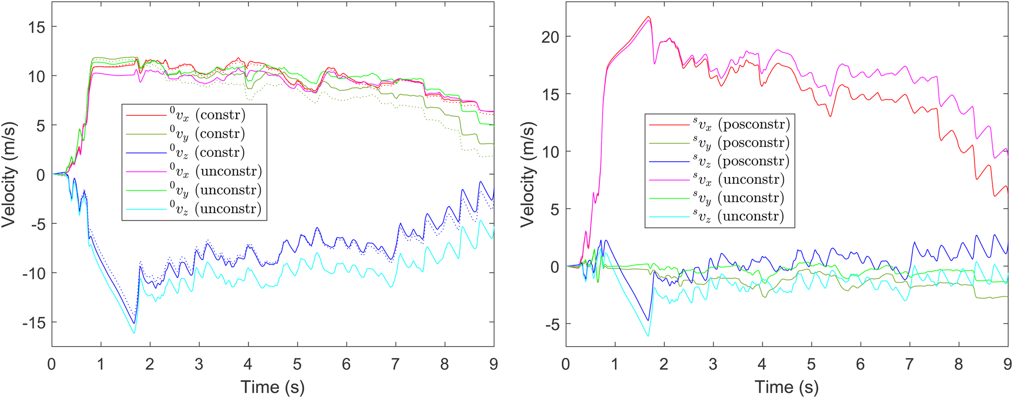
On the basis of supplementary Doppler radar measurements, the motion of the avalanche front has been determined. The observed signal is shown in the diagram in Figure 3, from which the range-time curve of the avalanche front can be deduced (as a step function), see also the right diagram of Figure 19. Accordingly, one single velocity value for each of the subsequent range gates is determined. The span of the recovered sensor unit trajectory covers five entire range gates, which are represented by black framed error boxes in the left diagram of Figure 19. The length of each box corresponds to the length of the range gate (≈25 m, each) and the width is given by the estimated accuracy of the velocity evaluation (≈±1.5 m s−1). For the representation in the diagram, position and length of each range gate as well as the measured velocity have been projected onto the slope secant.
Translational velocity components with respect to the slope frame vs. travelling distance s x (left) and the corresponding path-time diagram (right). Both diagrams provide a comparison with the Doppler radar results (gray domains): velocities (left) and range-time diagram of the avalanche front (right) projected on the terrain. The horizontal span of the error boxes and bars refers to the length of each range gate (≈25 m). The vertical span of the error boxes refers to the uncertainty of the velocity evaluation (≈±1.5 m s−1). Note that close to a travelling distance of 125 m (according to t ≈ 9 s) the data corruption occurs.

From the velocity evolution displayed in the left diagram of Figure 19, it can be seen that the
avalanche is in a decelerating phase already before the sensor unit is
entrained. It takes the sensor unit 10–20 m to reach a
velocity, which is similar to the one of the avalanche front
(≈20 m s${^{-1}}$ ), meaning that the sensor unit is
necessarily several metres (definitely less than a 25 m range gate)
behind the front at that instant. Subsequently, the sensor unit appears to
move roughly at the same decelerating speed as the avalanche front. After a
travelling distance of about 50 m, the sensor unit velocity seems to
decrease less than the frontal velocity, i.e. the sensor unit moves towards
the front, which it appears to reach after a travelling distance of
70–100 m. From then on, the sensor unit is expected to remain
close to the avalanche front for a while. This plausible scenario fits well
with the data presented in both diagrams of Figure 19. The comparison of sensor unit and frontal velocities
on the same range axis is justified by the observation that the maximum
distance between the sensor unit and the avalanche front is significantly
smaller than the length of a range gate. In addition, the diagram supports
the conclusion that the tracking procedure prior to recalibration
overestimates the longitudinal velocity significantly, whereas the
(‘constrained’) velocity according to in situ
calibration better fits to the radar data. After a travelling distance of
about 120 m (just before the onset of data corruption), the
constrained velocity drops below the radar velocity. This behaviour is
assessed to be unphysical and to originate from the escalating lateral drift
occurring close to the end of the processed time interval.
), meaning that the sensor unit is
necessarily several metres (definitely less than a 25 m range gate)
behind the front at that instant. Subsequently, the sensor unit appears to
move roughly at the same decelerating speed as the avalanche front. After a
travelling distance of about 50 m, the sensor unit velocity seems to
decrease less than the frontal velocity, i.e. the sensor unit moves towards
the front, which it appears to reach after a travelling distance of
70–100 m. From then on, the sensor unit is expected to remain
close to the avalanche front for a while. This plausible scenario fits well
with the data presented in both diagrams of Figure 19. The comparison of sensor unit and frontal velocities
on the same range axis is justified by the observation that the maximum
distance between the sensor unit and the avalanche front is significantly
smaller than the length of a range gate. In addition, the diagram supports
the conclusion that the tracking procedure prior to recalibration
overestimates the longitudinal velocity significantly, whereas the
(‘constrained’) velocity according to in situ
calibration better fits to the radar data. After a travelling distance of
about 120 m (just before the onset of data corruption), the
constrained velocity drops below the radar velocity. This behaviour is
assessed to be unphysical and to originate from the escalating lateral drift
occurring close to the end of the processed time interval.
6. Discussion
A consistent assessment of the presented results is a delicate issue since they refer to a unique dataset, which has required specific methods of evaluation, in particular, the in situ approach for sensor calibration. Suitable reference data, which could be applied for a validation of these methods, are difficult to obtain. As discussed in Section 5.1, the method of in situ calibration essentially relies on a peculiarity of the observed sensor unit motion: a sufficiently good conditioning of the equation system determining the calibration parameters is only achieved, if the ‘randomness’ of the involved rotations is sufficiently high. Accordingly, it would be extremely laborious to design and conduct a reference experiment to obtain a proper dataset for the validation procedure. The test device would have to reproduce a suitable type of rotational motion superimposed to a long-range translational motion. Moreover, the algorithms applied in the paper essentially rely on magnetometer data. To reproduce the characteristics of the field experiment, one would have to create a reference motion without inducing any (electro-)magnetic disturbances in the sensors. Under these circumstances, an automated guided motion can hardly be achieved. Simple rolling outdoors would not meet the requirements concerning the character of the rotational motion. Rotating by hand might be a possibility, however monitoring the rotational motion would require an additional measurement system, which would have to be validated itself.
Referring to these difficulties, we suggest to clearly distinguish between a conceptual validation on the one hand and an assessment of accuracy on the other. Specifically, our conceptual validation refers to the following aspects: the reliability of angular orientations is assessed by the degree of constancy of the global magnetic field components and by the reproducibility of the inclination. The conceptual integrity of the recovered trajectory is deduced form the correctly reproduced orientation of the initial motion sequence. Finally, the recovered velocity evolution is compared to the velocity of the avalanche front, which reveals a good coincidence immediately after the acceleration phase and yields a plausible interpretation of the sensor unit motion relatively to the avalanche front thereafter. Strictly speaking, the quoted criteria are necessary (but not sufficient) conditions for the integrity of the results. Arguments to further support the results are of rather qualitative nature: a closer investigation of the evolution of angular velocities and orientation in Section 4.2.2 reveals a plausible characteristic of the initial rotation sequence, which would not be expected if there is a relevant error in the angular orientations. A similar argument holds for the translational velocity components, treated in Section 5.2.3. Referring to a comment of one of the reviewers, it is mentioned that the terrain surface cannot be taken as a reference for the trajectory, since the related information is already essentially used for the in situ calibration.
Dealing with the question of accuracy, it has to be stated that the achieved long-term accuracy of the tracking procedure is rather poor. Owing to the well-discussed shortcomings of the data acquisition and, in particular, of the low sampling rate, this fits well to the expectations. It is emphasized that the heavy drift observed in the horizontal projection of the trajectory is not considered to conflict with the conceptual validation, but is rather considered a matter of low accuracy (due to the well-discussed reasons). Unfortunately, the well-known end position of the sensor unit can neither be applied to reduce the positioning error nor to provide for an assessment of the accuracy of the method, since we don't see a realistic chance to bridge the data gap (Section 3), which would allow to link the information about the initial and the final motion sequence.
A particularly interesting aspect of the recovered motion is related to the ballistic flight phases, reflected by a smooth parabolic trajectory, which proves that, in principle, the method is capable of quantitatively reproducing a transverse motion, i.e. a motion perpendicular to the terrain. In view of avalanche dynamics, this aspect is of particular interest, since no other experimental method for the observation of through-the-depth motion in an avalanche is known so far. Referring to a comment of one reviewer, it is noted that the observed transverse movement is, most likely, not directly related to the snow movement, since the sensor unit appears to be detached from the avalanche body. From a more fundamental point of view, the observation supports the underlying assumption that the constraint is not too restrictive, in the sense that it is capable of circumventing a numerical drift perpendicular to the terrain without suppressing physical motion in the same direction. This results, however, are of preliminary character until they will be reproduced by further experiments with a technologically advanced sensor equipment.
According to the nature of the tracking procedure, velocity results are more accurate than position results. At the present status of data evaluation, it appears that the information relevant for avalanche dynamics can be extracted from the recovered velocity evolution without further reference to the (less reliable) trajectory. This involves the motion of the sensor unit relatively to the avalanche front, which – in the present experiment – cannot be seen from other observations and – potentially – the detection and quantification of through-the-depth motion within the avalanche body, as well as the comparability with the results of alternative experimental methods such as radar velocity measurements, GNSS and radio ranging measurements, and, in particular, of numerical models.
7. Conclusion and outlook
The outcome of this paper is twofold: primarily, a real scale avalanche experiment is qualitatively and quantitatively analysed from different perspectives, involving in-flow measurements of inertial data, radar observations and GNSS positioning. To extract a maximum of information from the measurements, a number of ad hoc approaches were necessary to overcome several shortcomings associated with the lack of any in-field experience with the measurement set-up. From this, a secondary motivation arose, which gave rise to the development of a bundle of numerical methods for the processing of the specific inertial motion data.
It is demonstrated in principle that the applied sensor system is suited for the acquisition of in-flow data, which can be used for qualitative and quantitative motion analysis. The qualitative data analysis allows to clearly distinguish different flow phases of the sensor unit: rapid initial acceleration when being entrained at the avalanche front, steady flow movement superimposed with random jerks and short ballistic motion phases when being transported by the avalanche body, and rolling on the surface of the resting snow cover after being released from the bulk of moving snow.
The quantitative data analysis provides estimates of the evolution of the angular orientation, translational and angular velocity, as well as the trajectory of the sensor unit transported by the avalanche. To obtain plausible positioning results, a soft constraint condition is applied to recover the trajectory along the terrain surface. This approach is interpreted as a method of calibration, by which means the parameters of the accelerometer error model are determined such that the constraint condition is fulfilled in an averaged sense. The procedure is based solely on the data recorded in the course of the experiment. To account for this, the concept of in situ calibration is introduced. The constraint condition can be posed at a velocity level as well as at a position level. It turns out that both approaches yield similar results concerning position and translational velocity data. A detailed assessment regarding the numerical stability of the method suggests to prefer the position level approach.
Experiences gained from the single experiment revealed the need for further, repeated measurement campaigns with an advanced hardware. Such experiments have most recently highlighted the potential of state-of-the-art GNSS to track particle motion in snow avalanches (Neuhauser and others, Reference Neuhauser, Koehler, Neurauter, Adams and Fischer2023). As a next step, high-resolution motion tracking requires a fusion of inertial and GNSS data, where conventional methods of state estimation may benefit from the in situ calibration approach of the present work.
Supplementary material
The supplementary material for this article can be found at https://doi.org/10.1017/aog.2024.5.
Acknowledgements
This work was conducted as part of the international cooperation project ‘AvaRange - Particle Tracking in Snow Avalanches’ supported by the German Research Foundation (DFG, project No. 421446512) and the Austrian Science Fund (FWF, project No. I 4274-N29). Radar analysis was performed by Anselm Koehler, supported by the Swiss National Science Foundation (SNSF) project ‘Identify critical terrain features and flow states on surge formation in snow avalanches’ (P400P2_186687). Additional financial support came from the open Avalanche Framework AvaFrame (https://www.avaframe.org/), a cooperation between the Austrian Research Centre for Forests (BFW) and the Austrian Avalanche and Torrent Service (WLV) in conjunction with the Austrian Ministry of Agriculture, Forestry, Regions and Water Management (BML). The additional support of Christoph Hesselbach (GIS Evaluation) and particularly the avalanche experiment crew (SLF (Betty Sovilla) and Ski Patrol Davos-Klosters) is gratefully acknowledged.
Appendix A. Sensor calibration
It is a certain drawback of the present work that a proper calibration of IMU sensors has not been performed in temporal and spatial proximity of the field measurements. As it is generally the case for any measurement process, the IMU raw data are corrupted by systematic as well as stochastic sources of error. The former can be largely eliminated by standard methods of IMU sensor calibration. Assuming that the systematic errors are composed of a constant misalignment of sensor axes, constant scaling errors and constant offsets, linear calibration equations are obtained of the form

Therein,
$\tilde {\bf a} = [ \tilde a_x\; \tilde a_y\; \tilde a_z]$ is the vector of measured
acceleration components at a given time t and x
its improved counterpart, A the 3 × 3
calibration matrix and b the bias vector. Analogous error models
are assumed for angular velocity sensors (gyrometers) and magnetometers. The
calibration parameters (components of A and b) are
determined from reference measurements: for the accelerometer calibration,
earth's acceleration is taken as a reference and is measured utilizing
several different orientations of the sensor triad. While the magnitude of the
true acceleration is constant, the magnitude of the measured acceleration will
(slightly) differ from one orientation to another. An optimization procedure is
applied to determine the calibration parameters such that the deviation from the
true magnitude is minimum for all considered orientations in a least squares
sense. Details on the underlying numerical procedure can be found in, e.g.
Aggarwal and others (Reference Aggarwal, Syed, Niu and El-Sheimy2008) and
Stančin and Tomažič (Reference Stančin and Tomažič2014). Such reference measurements have been performed in 2018, i.e.
about 5 years after recording the field data at the Flüela Pass. Results
are shown at the top of Figure 20 where
raw data as well as calibrated data are drawn.
is the vector of measured
acceleration components at a given time t and x
its improved counterpart, A the 3 × 3
calibration matrix and b the bias vector. Analogous error models
are assumed for angular velocity sensors (gyrometers) and magnetometers. The
calibration parameters (components of A and b) are
determined from reference measurements: for the accelerometer calibration,
earth's acceleration is taken as a reference and is measured utilizing
several different orientations of the sensor triad. While the magnitude of the
true acceleration is constant, the magnitude of the measured acceleration will
(slightly) differ from one orientation to another. An optimization procedure is
applied to determine the calibration parameters such that the deviation from the
true magnitude is minimum for all considered orientations in a least squares
sense. Details on the underlying numerical procedure can be found in, e.g.
Aggarwal and others (Reference Aggarwal, Syed, Niu and El-Sheimy2008) and
Stančin and Tomažič (Reference Stančin and Tomažič2014). Such reference measurements have been performed in 2018, i.e.
about 5 years after recording the field data at the Flüela Pass. Results
are shown at the top of Figure 20 where
raw data as well as calibrated data are drawn.
Laboratory calibration of accelerometers (top) and gyrometers (bottom): Uncalibrated (left) versus calibrated data (right). While the effect of calibration is apparent in the case accelerometers, it is marginal in the case of gyrometers.

The calibration of gyrometers is performed on the basis of a reference motion generated by an industrial robot Stäubli TX2-90L. It can be seen from Figure 20 (bottom) that the quality of the gyrometer data is high even before the calibration, such that the effect of the calibration is marginal (but existent).
In the case of magnetometer calibration, a different strategy is pursued which is described in Renaudin and others (Reference Renaudin, Afzal and Lachapelle2010). The magnetometer data, and thus a reliable calibration of sensors, are crucial for the correct determination of angular orientation. The particular advantage of the chosen approach is that it allows to perform the calibration on the basis of the field data. This has become necessary since it turned out that the calibration of 2018, having been performed under laboratory conditions, is not valid for the field data of 2013, which can be seen from the bottom-right diagram of Figure 21: the avalanche data, subjected to the laboratory calibration, do not fit to the sphere, meaning that the magnitude of the measured magnetic field is not constant while the sensors are rotating.
Top-left, top-right, bottom-left: Magnetic field data recorded in the course of the 2013 Flüela experiment subjected to in situ calibration. Bottom-right: The same data subjected to laboratory calibration of 2018.
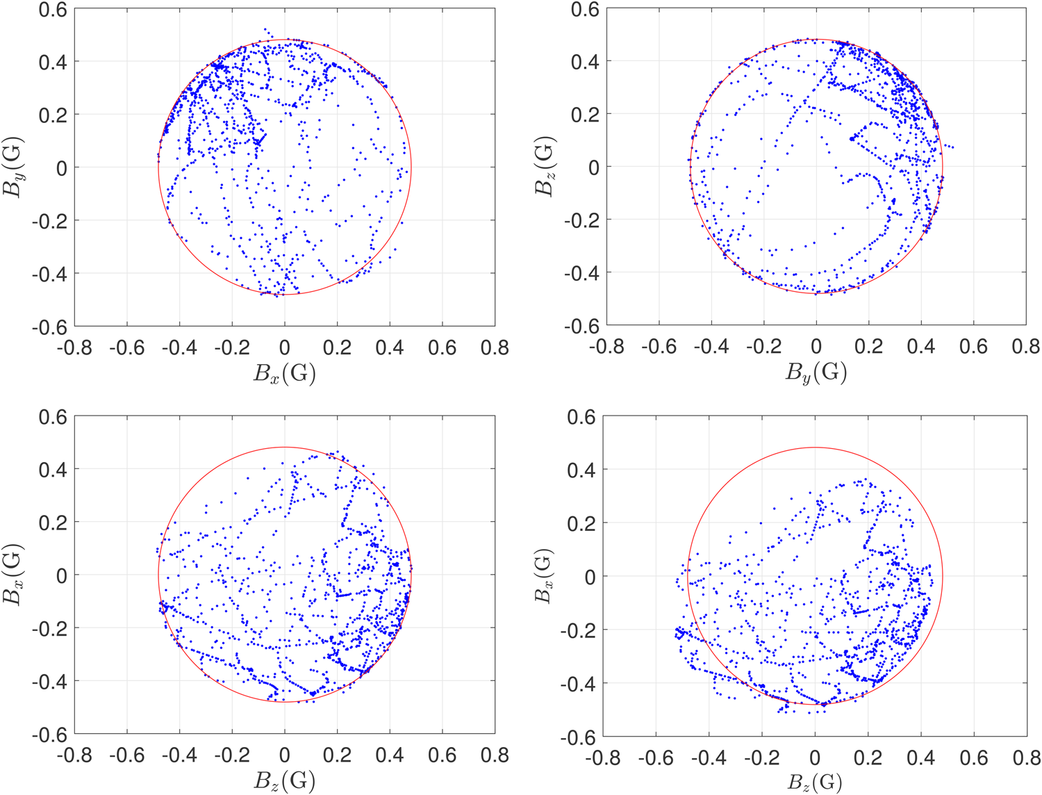
The idea of the calibration procedure is to record a time series of magnetic field vectors 1B(t n) = [ 1B x(t n) 1B y(t n) 1B z(t n) ]T while rotating the sensor triad in a more or less arbitrary way. At the absence of (electro-)magnetic disturbances and assuming that the 1B i are ideal measurements, the tips of vectors 1B lie on a sphere with a radius that corresponds to the strength of Earth's magnetic field (≈0.48 Gs). In the case of real measurements, this sphere shifts (hard iron distortion), deforms (soft iron distortion) and is superimposed by a basically random noise. Assuming that the transformation composed of a deformation and a shift is linear and constant in time, the deformed surface is an ellipsoid, and calibration equation (A.1) again applies. The calibration parameters, i.e. the components of the corresponding calibration matrix and bias vector, are obtained by fitting an ellipsoid to the measured data points. This procedure works best if the data points are uniformly distributed over the sphere/ellipsoid. This can be achieved to a certain degree in the course of laboratory calibration.Footnote 14 In the present case of in situ calibration, the data points reflect the actual rotational motion of the sensor in the course of the Flüela experiment: as can be expected, their distribution is by far not uniform. It turns out, however, that this kind of distribution is appropriate to achieve a sufficient accuracy of the calibration:
From what has been said before it can be deduced that the quality of the calibration can be assessed by the degree of non-constancy of ||1B(t)|| or by the size of the deviation of the dataset from an ideal sphere. The latter criterion is even more significant, since the spread of the data is also apparent in the corresponding diagram. Dealing with the Flüela data, the bottom-right diagram in Figure 21 demonstrates the situation according to the laboratory calibration: the deviation from spherical shape is apparent, which implies that the laboratory calibration is not consistent with the in-field data. After recalibration on the basis of the in-field data (in situ calibration), the deviation is largely reduced and dominated by basically random noise (bottom-left diagram), although the distribution of the data point is not uniform. The diagrams at the top of the figure demonstrate the same aspect but with respect to different coordinate sections. Concluding, the quality of the achieved recalibration is assessed as adequate in the sense that the low-frequency variation of ||1B(t)|| is smaller than the super-imposed random noise magnitude, which can be seen from the diagrams.
Appendix B. Replacement of deficient gyrometer data
The Flüela IMU data come along with the problem that the observed angular
velocities have occasionally exceeded the measurement range of the gyroscopes
($\pm \, 300^\circ /$ s−1,
nominally). At several instances, only two out of the three angular velocity
components 1ω 1,
1ω 2,
1ω 3 are available (Fig. 6). However, the missing component(s)
can be recovered with the help of the magnetometer data, as long as there is at
least one component available. The corresponding procedure, which has been used
in the present work, is described in the following.
s−1,
nominally). At several instances, only two out of the three angular velocity
components 1ω 1,
1ω 2,
1ω 3 are available (Fig. 6). However, the missing component(s)
can be recovered with the help of the magnetometer data, as long as there is at
least one component available. The corresponding procedure, which has been used
in the present work, is described in the following.
The three magnetometers measure the components
1B k of
earth's magnetic field B with respect to the corotational
sensor coordinate system
$( {\bf e}^1_1,\; \, {\bf e}^1_2,\; \, {\bf e}^1_3)$ . That is,

Denoting the effective angular velocity vector
by ω* (to be distinguished from the
measured one), one has
$\dot {\bf e}^1_k = {\boldsymbol \omega }\times {\bf e}^1_k$ (Wittenburg, Reference Wittenburg2008). Since B is constant,

with
$\tilde {\bf B}$ being the skew-symmetric matrix
related to the vector B. Equation (B.2), for k = 1,
2, 3, can be interpreted as a system of equations constraining
the 1ω k,
being the skew-symmetric matrix
related to the vector B. Equation (B.2), for k = 1,
2, 3, can be interpreted as a system of equations constraining
the 1ω k,
Unfortunately, this system is underdetermined, which has a simple geometric
reason: a rotation about the direction of the B vector does
not affect the corotational coordinates
${}^1\!\dot {B}_k$ . However, the three equations (B.2) can be enriched by obvious
additional equations to obtain an overdetermined system
. However, the three equations (B.2) can be enriched by obvious
additional equations to obtain an overdetermined system

To
ensure a favourable conditioning of system (B.3), the components of the magnetic field have been
normalized, i.e.
${}^1\!\hat {B}_k = {}^1\!B_k/\Vert {\bf B}\Vert$ , where ||B|| is the
constant magnitude of earth's magnetic field. If, at a certain instant,
one or two of the measured angular rates
1ω k
is/are missing, the respective line(s) in system (B.3) is/are simply eliminated. The time derivatives of
the normalized magnetic field components at time step n,
${}^1\dot {\hat {{\bf B}}}_n = [ \, {}^1\!\dot {\hat {B}}_1^{( n) }\; \; {}^1\!\dot {\hat {B}}_2^{( n) }\; \; {}^1\!\dot {\hat {B}}_3^{( n) }\, ] ^T$
, where ||B|| is the
constant magnitude of earth's magnetic field. If, at a certain instant,
one or two of the measured angular rates
1ω k
is/are missing, the respective line(s) in system (B.3) is/are simply eliminated. The time derivatives of
the normalized magnetic field components at time step n,
${}^1\dot {\hat {{\bf B}}}_n = [ \, {}^1\!\dot {\hat {B}}_1^{( n) }\; \; {}^1\!\dot {\hat {B}}_2^{( n) }\; \; {}^1\!\dot {\hat {B}}_3^{( n) }\, ] ^T$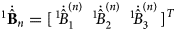 , are estimated by means of the
symmetric difference quotient
, are estimated by means of the
symmetric difference quotient

for n ≥ 1. For the first (n = 0) and the last time step the right and the left difference quotients, respectively, are used instead.


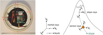

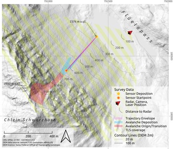
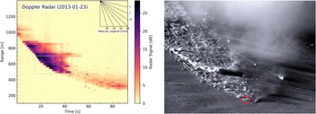


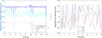
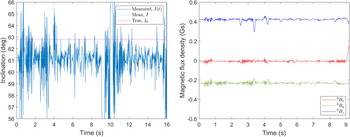

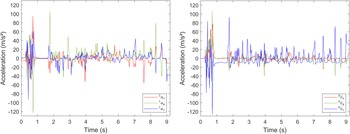

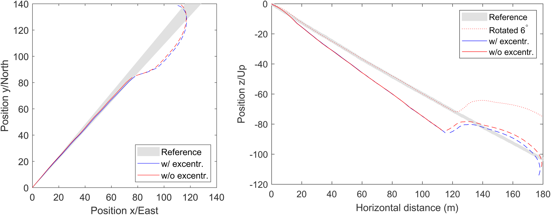
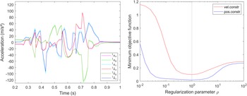

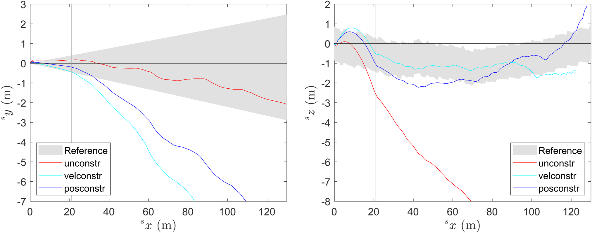


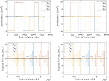


 Open access