





1 Introduction
Laser–target interactions can generate intense electromagnetic pulses (EMPs) in the GHz and THz frequency bands, which can interfere with measurements or damage components of the laser or diagnostics. This risk is partially mitigated with shielding to minimize electromagnetic interference (EMI), but EMPs remain a significant concern in many high-energy laser facilities and are poised to become an even larger issue in the next generation of ultra-high-intensity lasers.
EMPs are generated when electrons are ejected from the target by the laser[
Reference Consoli, Tikhonchuk, Bardon, Bradford, Carroll, Cikhardt, Cipriani, Clarke, Cowan, Danson, De Angelis, De Marco, Dubois, Etchessahar, Garcia, Hillier, Honsa, Jiang, Kmetik, Krása, Li, Lubrano, McKenna, Metzkes-Ng, Poyé, Prencipe, Raczka, Smith, Vrana, Woolsey, Zemaityte, Zhang, Zhang, Zielbauer and Neely
1
, Reference Dubois, Lubrano-Lavaderci, Raffestin, Ribolzi, Gazave, Compant La Fontaine, d’Humières, Hulin, Nicola, Poyé and Tikhonchuk
2
]. In a simple one-dimensional (1D) model, an expanding electron sheath of charge
$-2\sigma$
 is followed by an ion front of charge
$\sigma$
is followed by an ion front of charge
$\sigma$
 , leaving a remaining positive charge
$\sigma$
, leaving a remaining positive charge
$\sigma$
 on the target[
Reference Mora
3
]. This system can be approximated by an electric dipole with
$\sigma$
on the target[
Reference Mora
3
]. This system can be approximated by an electric dipole with
$\sigma$
 on the target and
$-\sigma$
on the target and
$-\sigma$
 in the expanding plasma, whose field determines the potential on the target. Above threshold laser intensities (typically
$\gtrsim {10}^{14}$
in the expanding plasma, whose field determines the potential on the target. Above threshold laser intensities (typically
$\gtrsim {10}^{14}$
 W/cm
${}^2$
W/cm
${}^2$
 ), ‘hot’ electrons are produced near the target surface by laser plasma instabilities (LPIs) such as two-plasmon decay (TPD) and stimulated Raman scattering (SRS). At even higher intensities (
$\gtrsim {10}^{18}$
), ‘hot’ electrons are produced near the target surface by laser plasma instabilities (LPIs) such as two-plasmon decay (TPD) and stimulated Raman scattering (SRS). At even higher intensities (
$\gtrsim {10}^{18}$
 W/cm
${}^2$
W/cm
${}^2$
 ), additional mechanisms accelerate electrons to even higher energies[
Reference Rusby, Kemp, Wilks, Miller, Sherlock, Chen, Simpson, Mariscal, Swanson, Djordjević, Link, Williams and Mackinnon
4
]. Energetic electrons produced by any of these mechanisms can easily escape the target dipole potential, and in doing so leave an additional positive charge on the target.
), additional mechanisms accelerate electrons to even higher energies[
Reference Rusby, Kemp, Wilks, Miller, Sherlock, Chen, Simpson, Mariscal, Swanson, Djordjević, Link, Williams and Mackinnon
4
]. Energetic electrons produced by any of these mechanisms can easily escape the target dipole potential, and in doing so leave an additional positive charge on the target.
On short (ps) time scales, the accelerating electric dipole moment radiates EMPs in the THz band[ Reference Consoli, Tikhonchuk, Bardon, Bradford, Carroll, Cikhardt, Cipriani, Clarke, Cowan, Danson, De Angelis, De Marco, Dubois, Etchessahar, Garcia, Hillier, Honsa, Jiang, Kmetik, Krása, Li, Lubrano, McKenna, Metzkes-Ng, Poyé, Prencipe, Raczka, Smith, Vrana, Woolsey, Zemaityte, Zhang, Zhang, Zielbauer and Neely 1 ]. On longer (ns) timescales, the remaining target potential is neutralized by a return current that is typically drawn up the structure supporting the target, typically a thin stalk[ Reference Sinenian, Manuel, Frenje, Séguin, Li and Petrasso 5 ]. For typical stalk dimensions, this current radiates EMPs in the GHz band. The magnitude of the GHz EMP should therefore be proportional to the target potential.
Recent experiments at the OMEGA Laser Facility[
Reference Cufari, Johnson, Li, Frenje, Moloney, Crilly, Heuer and Davies
6
] have demonstrated that applying a 10 T magnetic field to a spherical implosion significantly reduces the target potential (measured at the implosion bangtime). As a plasma expands into a background magnetic field, the diamagnetic current
$J=\nabla p\times B/{B}^2$
 and the
$\overrightarrow{E}\times \overrightarrow{B}$
and the
$\overrightarrow{E}\times \overrightarrow{B}$
 drift because the ambipolar field from charge separation expels the magnetic field, forming a diamagnetic cavity and a region of compressed field[
Reference Collette and Gekelman
7
, Reference Winske, Huba, Niemann and Le
8
]. The resulting magnetic field decreases away from the target surface, then increases at the edge of the cavity, creating a magnetic mirror that focuses a portion of hot electrons (generated by LPI) back onto the target where they collide and recombine, reducing the target charge. We hypothesized that the magnitude of the GHz EMP should also be reduced, and that the increasing number of electron–target collisions would also lead to an increase in hard X-ray emission on magnetized shots.
drift because the ambipolar field from charge separation expels the magnetic field, forming a diamagnetic cavity and a region of compressed field[
Reference Collette and Gekelman
7
, Reference Winske, Huba, Niemann and Le
8
]. The resulting magnetic field decreases away from the target surface, then increases at the edge of the cavity, creating a magnetic mirror that focuses a portion of hot electrons (generated by LPI) back onto the target where they collide and recombine, reducing the target charge. We hypothesized that the magnitude of the GHz EMP should also be reduced, and that the increasing number of electron–target collisions would also lead to an increase in hard X-ray emission on magnetized shots.
Applying a magnetic field to a target also constrains the expansion of the laser-produced plasma perpendicular to the field[ Reference Harilal, Tillack, O’Shay, Bindhu and Najmabadi 9 ]. The potential on the target due to the dipole field is proportional to the dipole moment, which in this case is the distance between the target and the expanding plasma. Therefore, we expect the target potential due to this dipole moment to be decreased by a magnetic field applied parallel to the target surface. In general, we hypothesize that the target potential is set by this dipole moment in the absence of hot electrons, but is dominated by the charge left by hot electrons in experiments where they are produced.
In this paper we present results from three sets of experiments. In the first (Section 2), on the OMEGA laser, we confirm that the GHz EMP generated in spherical implosion experiments in an intensity regime where hot electrons determine the target potential is indeed suppressed by an applied magnetic field. In the second experiment (Section 3, on the Peening laser at the University of California Los Angeles (UCLA) Phoenix Laser Facility), we show that this effect is also observed at much lower intensities where hot electrons are not generated, with lower field strengths and in planar geometry. In the third (Section 4), on the OMEGA EP laser, we observe that the EMP is actually enhanced by an applied magnetic field at high laser intensities (
$\sim {10}^{19}$
 W/cm
${}^2$
W/cm
${}^2$
 ) with a correspondingly hot electron population (
$\ge 1$
) with a correspondingly hot electron population (
$\ge 1$
 MeV). We conclude in Section 5.
2 Spherical implosions
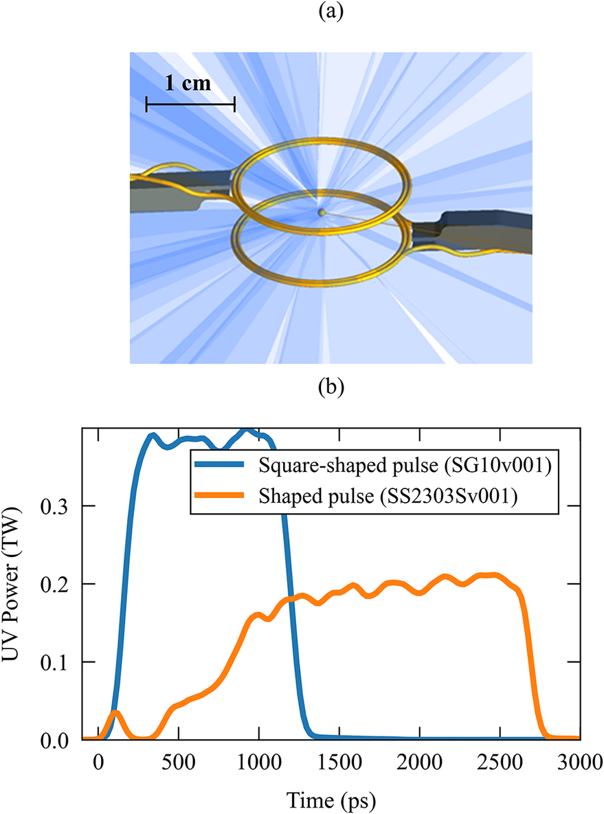
EMP measurements were collected by a magnetic flux probe on four campaigns studying magnetized spherical implosions at the OMEGA Laser Facility (Figure 1). Two shot days with the MagImp platform used 1-ns square-shaped pulses with total energies ranging from 10 to 25 kJ ((0.5–1)
$\times {10}^{15}$
 W/cm
${}^2$
W/cm
${}^2$
 ) to implode approximately 850 μm outer diameter (OD), 2.5 μm thick glass shells. Two other shot days with the MagMix and MagSDD platforms used a 20–23 kJ shaped pulse to implode 880 μm OD, 23.4 μm thick CH shells. The MagMix shot day tested both 1 ns square pulses and a shaped pulse comprising a picket followed by a flat top drive (Figure 1(b)). The MagSDD shot day used the same shaped pulse on all shots. In this regime, hot electrons are generated near the target quarter-critical surface by TPD. In all four experiments, a subset of shots was magnetized using a set of Helmholtz coils pulsed by the magneto-inertial fusion electrical discharge system (MIFEDS)[
Reference Fiksel, Agliata, Barnak, Brent, Chang, Folnsbee, Gates, Hasset, Lonobile, Magoon, Mastrosimone, Shoup and Betti
10
], providing a peak magnetic field of 10 T for the MagImp platform and 12 T for the MagMix and MagSDD platforms. The MIFEDS current pulse is sinusoidal with an approximately 1 μs rise time, so the applied field is effectively static over the duration of the experiment (several ns).
) to implode approximately 850 μm outer diameter (OD), 2.5 μm thick glass shells. Two other shot days with the MagMix and MagSDD platforms used a 20–23 kJ shaped pulse to implode 880 μm OD, 23.4 μm thick CH shells. The MagMix shot day tested both 1 ns square pulses and a shaped pulse comprising a picket followed by a flat top drive (Figure 1(b)). The MagSDD shot day used the same shaped pulse on all shots. In this regime, hot electrons are generated near the target quarter-critical surface by TPD. In all four experiments, a subset of shots was magnetized using a set of Helmholtz coils pulsed by the magneto-inertial fusion electrical discharge system (MIFEDS)[
Reference Fiksel, Agliata, Barnak, Brent, Chang, Folnsbee, Gates, Hasset, Lonobile, Magoon, Mastrosimone, Shoup and Betti
10
], providing a peak magnetic field of 10 T for the MagImp platform and 12 T for the MagMix and MagSDD platforms. The MIFEDS current pulse is sinusoidal with an approximately 1 μs rise time, so the applied field is effectively static over the duration of the experiment (several ns).
(a) Three-dimensional (3D) model of the MagSDD platform showing two MIFEDS coils in a Helmholtz configuration around a capsule illuminated by 60 beams. (b) Representative examples of the two laser pulse shapes used in the experiments.

Figure 1 Long description
Panel a shows a 3 D model. At the center is a small spherical capsule. Radiating outward from this capsule are 60 light blue beams. Surrounding the capsule are two parallel golden M I F E D S coils in a Helmholtz configuration. The coils are connected to grey and yellow electrical leads on the left and right sides. A scale bar in the top left indicates 1 cm.
Panel b is a line graph. The x-axis is Time in p s ranging from 0 to 3000. The y-axis is U V Power in T W ranging from 0.0 to 0.3. Two data series are plotted.
• The Square-shaped pulse S G 10 v 001 is a blue line that rises sharply at 100 p s, plateaus at approximately 0.38 T W with minor oscillations, and drops sharply to zero at 1300 p s.
• The Shaped pulse S S 2303 S v 001 is an orange line that shows a small initial peak at 100 p s, stays low until 400 p s, then rises in a stepped fashion to a plateau of approximately 0.2 T W between 1500 and 2600 p s before dropping to zero.
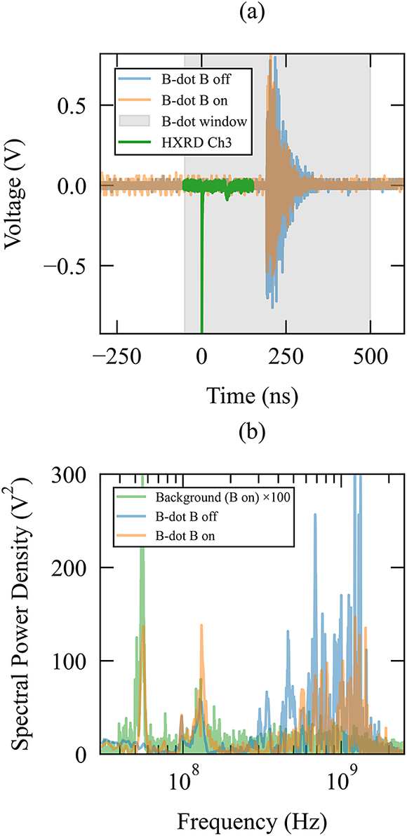
Electromagnetic waves generated by experiments on the OMEGA laser were measured by a magnetic flux or ‘B-dot’ probe routinely fielded as part of the EMP monitor (EMPMON) diagnostic. This Prodyn RB-130 B-dot probe is responsive up to 2 GHz and is inserted inside the target chamber 131 cm from the center. Several typical B-dot signals are shown in Figure 2(a). While the laser pulse is only 1 ns long, the EMP signal is longer duration, decaying away exponentially with a time constant of
$\tau =34$
 ns, which is a combination of the RC time constant of the stalk discharge current and the resonant modes of the spherical vacuum chamber.
(a) Raw B-dot (blue, orange) and hard X-ray diode (green) traces from an unmagnetized shot and a magnetized shot with the MagImp platform. The shaded region shows the time region that was included in the analysis. The X-ray data shown are from the unmagnetized shot: the magnetized signal is indistinguishable on this scale. (b) The spectral power density of the B-dot signal within the selected time range from the same two shots.

Figure 2 Long description
Panel a is a line graph with Time in n s on the x-axis from minus 250 to 500 and Voltage in V on the y-axis from minus 0.5 to 0.5. A light gray shaded region labeled B-dot window spans from approximately minus 50 to 500 n s. A green line representing H X R D Ch 3 shows a sharp negative spike at time zero. Two overlapping traces, B-dot B off in blue and B-dot B on in orange, remain flat until approximately 200 n s, where they both exhibit high-frequency oscillations peaking near 0.8 V before decaying by 400 n s.
Panel b is a semi-logarithmic plot with Frequency in H z on a log-scale x-axis from 10 super 7 to 10 super 9 and Spectral Power Density in V-squared on the y-axis from 0 to 300. Three traces are shown. Background B on times 100 in green shows a prominent peak near 5 times 10 super 7 H z. B-dot B off in blue shows multiple high-intensity peaks between 5 times 10 super 8 and 2 times 10 super 9 H z, with the highest peak reaching nearly 300 V-squared. B-dot B on in orange follows a similar profile but with significantly lower peak intensities, generally staying below 150 V-squared.
The power spectrum of the B-dot signal (Figure 2(b)) shows peaks near 0.1 GHz (
$\lambda \sim$
 3 m) and 1 GHz (
$\lambda \sim$
3 m) and 1 GHz (
$\lambda \sim$
 30 cm). We take the sum over the power spectrum from 1 MHz to 5 GHz as a metric for the total EMP energy on a shot. The background spectrum shown is taken from the portion of the magnetized signal prior to the laser shot. Based on the wavelengths, we identify the lower frequency peaks in the EMP spectrum as resonances of the target chamber (3.3 m OD) and the higher frequency peaks as emission from some portion of the target, target stalk and positioner. In the magnetized shots, the higher frequency emission is suppressed while some lower frequency modes are more strongly excited (Figure 2(b)). These peaks are due to the effect of the two MIFEDS units on the resonant modes of the chamber, as the MIFEDS units were not inserted on unmagnetized shots. Consequently, these peaks are also observed in the noise spectrum with the MIFEDS inserted (Figure 2(b)), while the noise spectrum on the unmagnetized shots without the MIFEDS (not shown) is flat.
To understand the variation in the experimental configurations, we consider the EMP generated on the unmagnetized shots across all experiments. Across all of these shots, the EMP metric varies by a factor of
$10\times$
 . Despite the variation in targets, the EMP metric varies by only a factor of
$2.5\times$
. Despite the variation in targets, the EMP metric varies by only a factor of
$2.5\times$
 for unmagnetized shots with 1 ns square-shaped pulses. Comparing shots with identical targets, the shots with the shaped pulse generated an order of magnitude fewer EMPs than those with the 1-ns square-shaped pulse. This is due to the significantly higher peak intensity of the square-shaped pulse compared to the shaped pulse (0.45 versus 0.18 TW), which results in more hot electron production.
Hard X-rays were diagnosed using the OMEGA hard X-ray detector (HXRD)[ Reference Stoeckl, Glebov, Meyerhofer, Seka, Yaakobi, Town and Zuegel 11 ], which consists of an array of four filtered channels, each with a scintillator coupled to a microchannel plate photomultiplier tube. We focused on the signals from channels 3 and 4, sensitive to more than 60 keV and more than 80 keV X-rays, respectively, which are associated with the stopping of hot electrons in the target. In these implosions X-rays produced by compression are negligible, so we assume that the entire HXRD signal is due to hot electrons and use the integral over the peak in the HXRD signal as a proxy for the number of hot electrons produced.
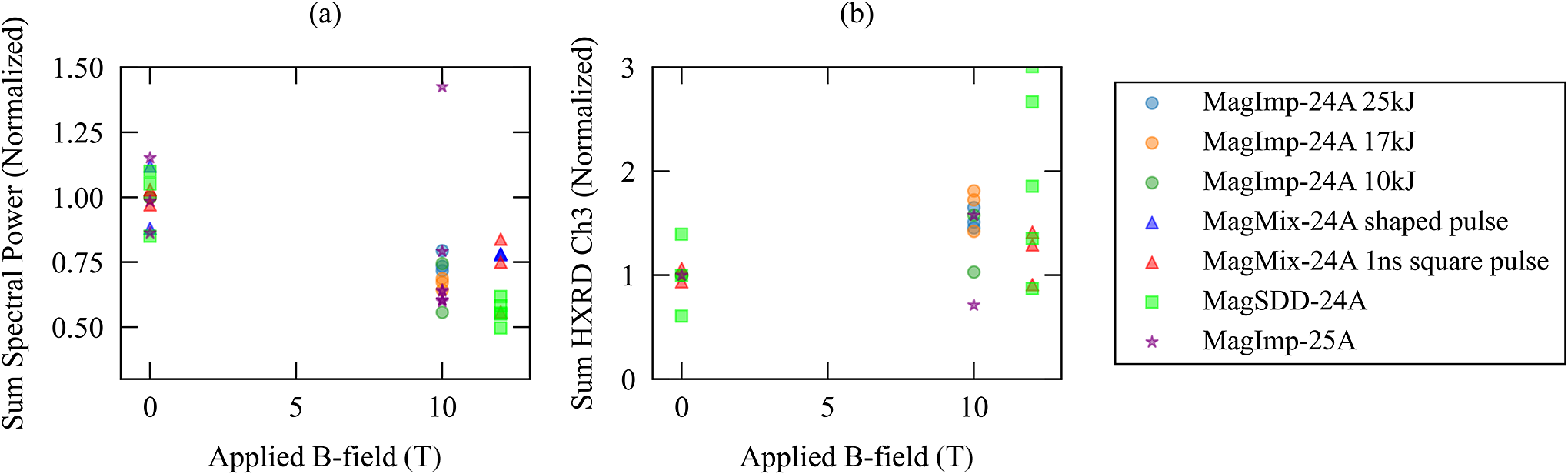
In order to compare the effect of the applied magnetic field across campaigns with different targets, laser energies and pulse shapes, we have divided the data into subsets of directly comparable shots. Within each subset, we normalized the EMP and HXRD metrics to the mean of the unmagnetized shots within that subset. The results are shown in Figure 3. By definition, the B = 0 T shots cluster around unity. The EMP metric clearly decreases with increasing magnetic field, while the HXRD metric increases.
(a) Total EMP (summed spectral power of the signal) and (b) total summed HXRD channel 3 (
$>60$
 keV) signal for each shot, each normalized to the mean of the directly comparable unmagnetized shots.

Figure 3 Long description
A two-panel scatter plot with a shared legend.
Panel a: The X-axis is labeled Applied B-field in T, with major ticks at 0, 5, and 10. The Y-axis is labeled Sum Spectral Power (Normalized), ranging from 0.50 to 1.50. Data points are clustered at 0 T and 10 T. At 0 T, most points cluster around 1.00. At 10 T, the points are generally lower, ranging between 0.50 and 0.85, with one outlier star symbol near 1.45.
Panel b: The X-axis is labeled Applied B-field in T, with major ticks at 0, 5, and 10. The Y-axis is labeled Sum H X R D Ch 3 (Normalized), ranging from 0 to 3. At 0 T, points cluster tightly around 1.0. At 10 T, there is a wider vertical spread, with most points between 1.0 and 2.0, and two green square outliers reaching near 2.7 and 3.0.
Legend on the right:
- Blue circle: MagImp-24A 25 k J
- Orange circle: MagImp-24A 17 k J
- Green circle: MagImp-24A 10 k J
- Blue triangle: MagMix-24A shaped pulse
- Red triangle: MagMix-24A 1 n s square pulse
- Green square: Mag S D D-24A
- Purple star: MagImp-25A
The mean and standard deviation of these normalized points for each magnetic field are presented in Table 1. We note that, within error, the HXRD and EMP metrics are inversely proportional, consistent with the model that electrons colliding with the target produce hard X-rays while simultaneously reducing the target charge and thus the potential energy that generates EMPs.
Mean value, standard error and sample sizes for the EMP measurement (sum spectral power) and HXRD channels 3 and 4 measurements (summed HXRD signal) normalized to the B = 0 T shots within each dataset.

Table 1 Long description
The table consists of six columns and four rows including the header.
Columns from left to right are:
1. B sub 0 (T): Magnetic field strength in Tesla.
2. E M P: Electromagnetic pulse measurement.
3. Number of E M P shots.
4. H X R D 3 (greater than 60 k e V): Hard X-ray detector channel 3.
5. H X R D 4 (greater than 80 k e V): Hard X-ray detector channel 4.
6. Number of H X R D shots.
Data rows:
- Row 1: B sub 0 is 0. E M P is 1.00 plus or minus 0.03 (13 shots). H X R D 3 is 1.00 plus or minus 0.06. H X R D 4 is 1.00 plus or minus 0.02 (9 shots).
- Row 2: B sub 0 is 10. E M P is 0.72 plus or minus 0.05 (15 shots). H X R D 3 is 1.45 plus or minus 0.10. H X R D 4 is 1.55 plus or minus 0.10 (10 shots).
- Row 3: B sub 0 is 12. E M P is 0.66 plus or minus 0.04 (11 shots). H X R D 3 is 1.67 plus or minus 0.26. H X R D 4 is 2.28 plus or minus 0.45 (8 shots).
The data shows that as B sub 0 increases, E M P values decrease while H X R D values increase.
3 Low-intensity planar targets
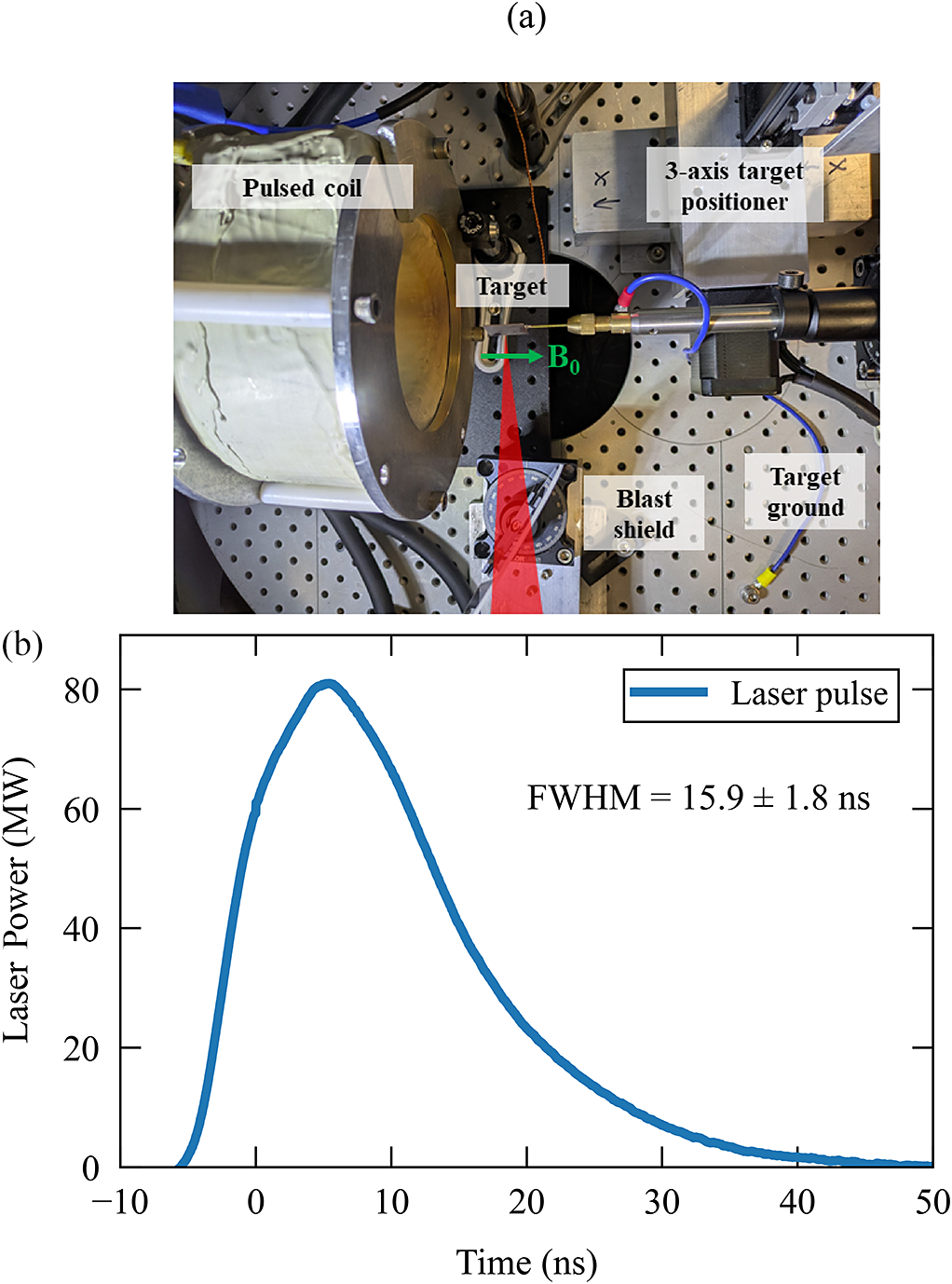
To investigate the suppression of EMPs by magnetic fields at much lower intensities, we conducted a series of shots at the Phoenix Laser Facility at the UCLA. The experimental setup is shown in Figure 4(a). The 1053 nm Peening laser[
Reference Hackel, Miller and Dane
12
] with an approximately 16 ns full width at half maximum (FWHM) Gaussian pulse shape (Figure 4(b)) was focused to a 40 μm FWHM spot on a planar 2 cm × 2 cm 500 μm thick copper target, tilted by approximately
$10{}^{\circ}$
 to avoid retro-reflection. Shots were taken with 1 and 4 J of laser energy,
$\pm$
to avoid retro-reflection. Shots were taken with 1 and 4 J of laser energy,
$\pm$
 5% ((5–20)
$\times {10}^{12}$
5% ((5–20)
$\times {10}^{12}$
 W/cm
${}^2$
W/cm
${}^2$
 ). This intensity is far below the thresholds for TPD and SRS, and so hot electrons are not generated at the target surface in this experiment.
(a) Photo of the setup with the magnetic field orientation, target position and beam path. (b) Average of the laser pulse throughout a run, as measured by a pick-off photodiode.

Figure 4 Long description
Panel a is a photo of an experimental setup on a breadboard. On the left is a large cylindrical Pulsed coil. To its right is the Target, positioned at the center of the frame. A green arrow labeled B sub 0 points right, indicating the magnetic field orientation. A red shaded cone represents the beam path hitting the target. Above the target is a 3-axis target positioner. Below the target is a Blast shield, and to the far right is the Target ground.
Panel b is a line graph titled Laser pulse. The x-axis is Time in n s, ranging from minus 10 to 50. The y-axis is Laser Power in M W, ranging from 0 to 80. A blue curve starts at 0 at approximately minus 5 n s, rises sharply to a peak of about 80 M W at 5 n s, and then decays asymptotically toward 0 by 50 n s. Text on the graph states F W H M equals 15.9 plus or minus 1.8 n s.
The target was soldered to an 8 cm long brass stalk, the base of which was connected to chamber ground by a wire. The target was mounted on a three-axis motion stage and was rastered between shots to present a fresh target surface, keeping the laser focus on the front of the target. A magnetic field of
${B}_0\sim 0.1$
 T was applied parallel to the target surface by a 40 turn coil pulsed at 2.5 kA and positioned 5 cm from the laser focus on the target. The current pulse is sinusoidal with a
$1.7$
T was applied parallel to the target surface by a 40 turn coil pulsed at 2.5 kA and positioned 5 cm from the laser focus on the target. The current pulse is sinusoidal with a
$1.7$
 ms rise time, so the field is effectively static over the duration of the experiment (tens of ns). The laser, target drive and coil pulser were operated at a 0.25 Hz repetition rate to collect datasets of several hundred shots.
On each shot, the EMP was measured with a Com-Power AH-118 double ridge guide horn antenna that was mounted on the outside of a plastic flange on the target chamber, approximately 38 cm from the center of the chamber, oriented perpendicular to the target stalk. The antenna is nominally sensitive over 0.7–18 GHz, although we measured signal down to
$0.4$
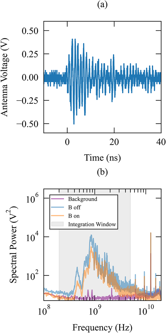
 GHz. The antenna signal was digitized with a Tektronix DPO72304SX (23 GHz, 50 GS/s) oscilloscope. Figure 5(a) shows a representative antenna signal from a single shot. No attempt is made to correct for the frequency response of the antenna or cables as these are assumed to be identical across all of the shots reported. Unlike in Section 2, the EMP signal is observed only while the laser is on.
(a) A raw single shot antenna trace from the unmagnetized run. (b) Median power spectra of the antenna signal across the magnetized and unmagnetized runs.

Figure 5 Long description
Panel a is a line graph of Antenna Voltage in Volts V on the y-axis versus Time in n s on the x-axis. The y-axis ranges from negative 0.50 to 0.50. The x-axis ranges from before 0 to 40. The trace shows a high-frequency oscillation that begins near 0 n s, reaching peak amplitudes of approximately 0.4 V before gradually decaying toward the baseline by 40 n s.
Panel b is a log-log line graph of Spectral Power in V squared on the y-axis versus Frequency in H z on the x-axis. The y-axis ranges from 10 super 0 to 10 super 6. The x-axis ranges from 10 super 8 to 10 super 10. A legend identifies four elements. A purple line for Background, a blue line for B off, an orange line for B on, and a light gray shaded region for the Integration Window. The Background remains flat near 10 super 1. Both B off and B on traces show a broad peak between 5 times 10 super 8 and 5 times 10 super 9 H z, contained within the shaded Integration Window. The B off signal is consistently higher in power than the B on signal within this window. A sharp narrow peak appears for both near 1.2 times 10 super 10 H z.
Figure 5(b) shows the median power spectra of the antenna signal during two of the runs. Again two peaks are evident: we identify the peak at approximately 0.5 GHz with resonances within the 75 cm OD spherical vacuum chamber and the peak at approximately
$0.8{-}2$
 GHz as emission from the target and stalk. Again, the background power spectrum is taken from the signal prior to the laser shot. The chamber modes are not evident in the background on this experiment, possibly because the antenna is just outside the chamber. We use the summed spectral power over the gray window marked in Figure 5(b) to represent the total EMP energy as a single scalar. Narrow peaks at more than 5 GHz do not change between shots and are evident in the background spectrum, and so these are attributed to resonances in the antenna circuit. When the magnetic field is applied, there is a clear reduction in magnitude across the spectrum, while its shape is unchanged.
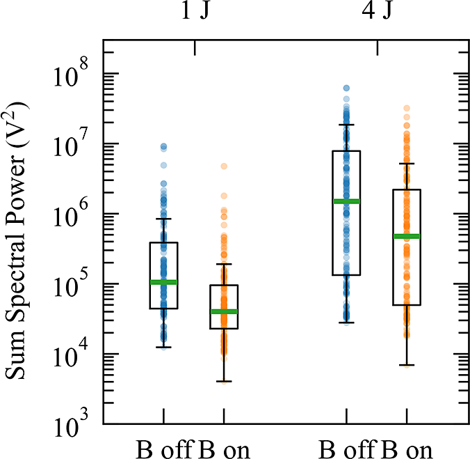
Two sequences of 100 shots each were collected both with and without the applied magnetic field, for a total of 400 shots, at each of two laser energies (1 and 4 J). A significant amount of shot-to-shot variation was observed on these runs, as evident in the distribution of the summed spectral power for each shot shown in Figure 6. This variation is likely due to fluctuations in the laser intensity on target, which have a strong impact on electron emission and consequently the EMP. The Peening laser has no beam smoothing, so hot spots of higher intensity occur randomly on each shot. It is also possible that imperfections in the target surface or the position as the target was rastered modified the intensity. However, both of these effects were stochastic, leading to similar distributions in the magnetized and unmagnetized runs.
Distribution of summed spectral powers from each shot showing that despite significant variability, there is a clear reduction in EMP power with the magnetic field applied. The boxes mark the first and third quartiles, the whiskers extend
$1.5$
 interquartile range (IQR) above and below the first and third quartiles, respectively, and the horizontal green lines mark the mean.

Figure 6 Long description
A logarithmic box and whisker plot. The vertical y-axis is labeled Sum Spectral Power in V super 2, ranging from 10 super 3 to 10 super 8. The horizontal x-axis is divided into two main categories: 1 J on the left and 4 J on the right. Each category contains two data sets: B off (blue points) and B on (orange points).
* In the 1 J category, the B off data is centered around a green mean line at approximately 10 super 5. The B on data shows a downward shift, with the mean line falling below 10 super 5 and a lower overall distribution of points.
* In the 4 J category, the B off data has a mean line slightly above 10 super 6. The B on data again shows a clear reduction, with the mean line dropping to approximately 5 times 10 super 5.
In all cases, the boxes represent the first and third quartiles, black whiskers extend to 1.5 times the I Q R, and individual data points are overlaid as semi-transparent circles showing significant vertical spread and overlap between conditions.
Comparing the distribution of the data in Figure 6 shows a clear suppression of the EMP. Using the two-sample Kolmogorov–Smirnov test, the B-on data cannot be consistent with the B-off distribution (
$p<0.1$
 %) in either the 1 or 4 J dataset. The suppression ratios are
$0.38\times$
%) in either the 1 or 4 J dataset. The suppression ratios are
$0.38\times$
 and
$0.32\times$
and
$0.32\times$
 for the 1 and 4 J datasets, respectively.
4 High-intensity planar targets
Since the magnitude of the EMP is correlated with laser intensity[
Reference Consoli, Tikhonchuk, Bardon, Bradford, Carroll, Cikhardt, Cipriani, Clarke, Cowan, Danson, De Angelis, De Marco, Dubois, Etchessahar, Garcia, Hillier, Honsa, Jiang, Kmetik, Krása, Li, Lubrano, McKenna, Metzkes-Ng, Poyé, Prencipe, Raczka, Smith, Vrana, Woolsey, Zemaityte, Zhang, Zhang, Zielbauer and Neely
1
], it is a particular threat to high-intensity (
$>{10}^{18}$
 W/cm
${}^2$
W/cm
${}^2$
 ) laser facilities, which can produce hot electrons with temperatures in the range 0.1–10 MeV[
Reference Rusby, Kemp, Wilks, Miller, Sherlock, Chen, Simpson, Mariscal, Swanson, Djordjević, Link, Williams and Mackinnon
4
]. We compared data from two shot days on two distinct platforms on OMEGA EP to assess the impact of magnetic fields on EMPs in this regime.
) laser facilities, which can produce hot electrons with temperatures in the range 0.1–10 MeV[
Reference Rusby, Kemp, Wilks, Miller, Sherlock, Chen, Simpson, Mariscal, Swanson, Djordjević, Link, Williams and Mackinnon
4
]. We compared data from two shot days on two distinct platforms on OMEGA EP to assess the impact of magnetic fields on EMPs in this regime.
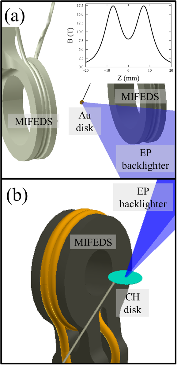
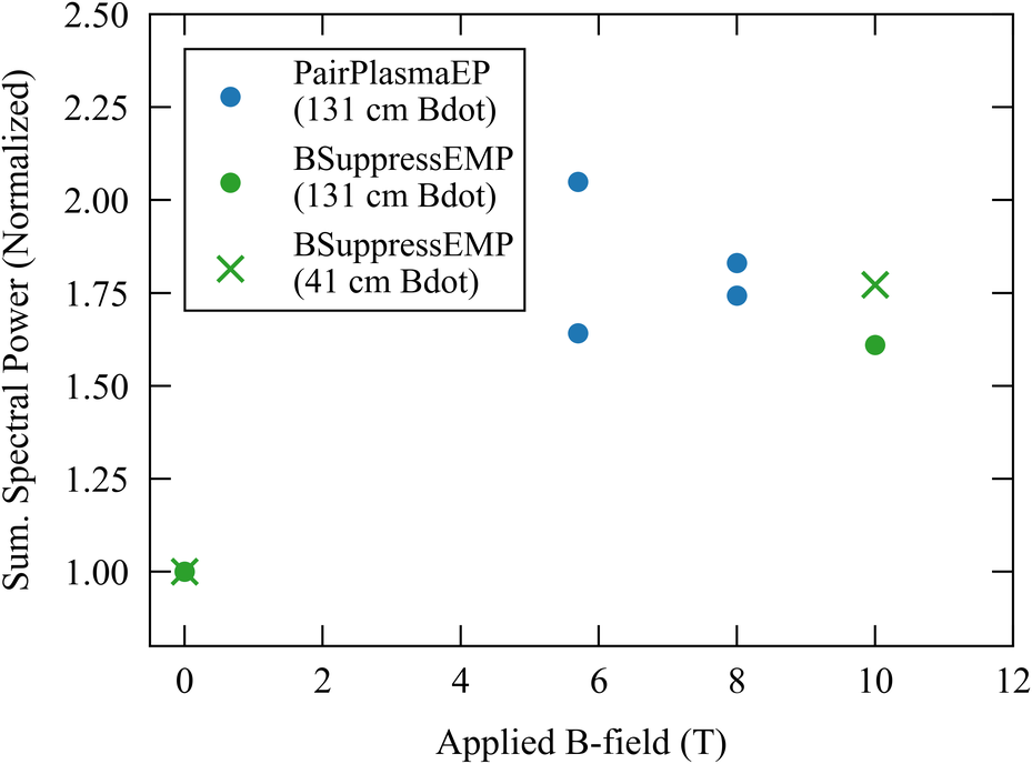
In the first experiment, named PairPlasmaEP (Figure 7(a)), the target was a 500 μm OD, 20 μm thick Au disk. The disk was shot with the OMEGA EP backlighter beam (
$\lambda =1054$
 nm) with a 10 ps FWHM pulse and an energy of 880–900 J (
$9\times {10}^{18}$
nm) with a 10 ps FWHM pulse and an energy of 880–900 J (
$9\times {10}^{18}$
 W/cm
${}^2$
W/cm
${}^2$
 ). The target was centered between a pair of MIFEDS coils, generating a field of up to 8 T parallel to the target surface. Two shots each were taken with magnetic field strengths of 5.7 and 8 T, along with one unmagnetized reference shot. The MIFEDS coils were not inserted on the unmagnetized reference shot. The intended purpose of the experiment was to trap electron–positron pairs in this magnetic mirror configuration, and particle tracing simulations and spectrometer measurements suggested that electrons and positrons up to 2.5 MeV are confined for up to 1 ns[
Reference der Linden, Fiksel, Peebles, Edwards, Willingale, Link, Mastrosimone and Chen
13
].
). The target was centered between a pair of MIFEDS coils, generating a field of up to 8 T parallel to the target surface. Two shots each were taken with magnetic field strengths of 5.7 and 8 T, along with one unmagnetized reference shot. The MIFEDS coils were not inserted on the unmagnetized reference shot. The intended purpose of the experiment was to trap electron–positron pairs in this magnetic mirror configuration, and particle tracing simulations and spectrometer measurements suggested that electrons and positrons up to 2.5 MeV are confined for up to 1 ns[
Reference der Linden, Fiksel, Peebles, Edwards, Willingale, Link, Mastrosimone and Chen
13
].
Computer-aided design (CAD) models of the (a) PairPlasmaEP and (b) BSuppressEMP experiments conducted on OMEGA EP. The inset plot in (a) shows the axial magnetic field profile.

Figure 7 Long description
Panel a shows the PairPlasmaEP setup. On the left is a grey cylindrical M I F E D S coil. To its right, a small brown A u disk is positioned. A blue cone representing the E P backlighter originates from the right and points toward the disk. Above this is an inset line graph showing the axial magnetic field profile. The x-axis is Z in millimeters from minus 20 to 20. The y-axis is B in Tesla from 0 to 17.5. The curve shows two symmetric peaks of 17.5 Tesla at approximately Z equals minus 7 and positive 7 millimeters, with a central trough of 8 Tesla at Z equals 0.
Panel b shows the BSuppressEMP setup. A larger grey M I F E D S coil with orange internal winding is on the left. To its right, a teal C H disk is held by a thin rod. A blue E P backlighter beam enters from the top right, focusing onto the surface of the C H disk.
In the second experiment, named BSuppressEMP (Figure 7(b)), the target was a 2 mm OD 30 μm thick CH disk, with a magnetic field of 10 T parallel to the target surface generated by a single MIFEDS coil. The target was again shot with the OMEGA EP backlighter beam with a 10 ps FWHM pulse, but with a lower energy of 200 J (
$2\times {10}^{18}$
 W/cm
${}^2$
W/cm
${}^2$
 ). One magnetized and one unmagnetized shot were collected. The MIFEDS coils were inserted for both shots.
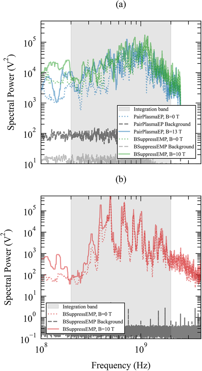
On both shot days, the EMP was measured by a Prodyn RB-130 B-dot probe (responsive to 2 GHz) positioned 131 cm from target chamber center (identical to the EMPMON used on OMEGA in Section 2). On the BSuppressEMP shot day, a second B-dot probe with a single 1 mm OD loop[ Reference Peebles, Davies, Barnak, Garcia-Rubio, Heuer, Brent, Spielman and Betti 14 ] was inserted 41 cm from chamber center. Example spectra are shown in Figure 8. As before, to compare data between the two different platforms and probes, the summed spectral power is normalized to that of the corresponding unmagnetized reference shot. Once again the background is extracted from the portion of the signal prior to the shot. In this experiment the EMP is much more intense, requiring additional attenuation on the probes, which significantly decreased the background.
Representative power spectra of the B-dot signals from shots with the OMEGA EP backlighter beam from the (a) 131 cm and (b) 41 cm B-dot probes. An enhancement in the EMP in the magnetized shots is evident at lower frequencies below 1 GHz.

Figure 8 Long description
Two vertically stacked line graphs, labeled a and b. Both share a common x-axis at the bottom representing Frequency in Hertz on a logarithmic scale from 10 super 8 to 2 times 10 super 9. The y-axis for both is Spectral Power in V-squared on a logarithmic scale.
Panel a: Top graph for the 131 cm B-dot probe. The y-axis ranges from 10 super 1 to 10 super 5. A light gray shaded region, the Integration band, spans from approximately 2 times 10 super 8 to 1.5 times 10 super 9 Hertz.
* The PairPlasmaEP B equals 0 T (dotted blue) and B equals 13 T (solid blue) lines fluctuate between 10 super 3 and 10 super 5, peaking near 8 times 10 super 8 Hertz.
* The BSuppressEMP B equals 0 T (dotted green) and B equals 10 T (solid green) lines show higher power at low frequencies, with the solid green line staying above 10 super 4 below 3 times 10 super 8 Hertz.
* Background levels (dashed gray and solid light gray) remain flat near 10 super 2 and 10 super 1 respectively.
Panel b: Bottom graph for the 41 cm B-dot probe. The y-axis ranges from 10 super minus 1 to 10 super 5. The Integration band is identical to panel a.
* The BSuppressEMP B equals 10 T (solid red) line shows a significant enhancement over the B equals 0 T (dotted red) line, particularly between 10 super 8 and 4 times 10 super 8 Hertz, where it is nearly an order of magnitude higher.
* Both red lines show sharp peaks reaching 10 super 5 near 5 times 10 super 8 and 7 times 10 super 8 Hertz.
* The BSuppressEMP Background (dashed dark gray) is significantly lower, fluctuating between 10 super minus 1 and 10 super 0.
The results are summarized in Figure 9. In stark contrast with the previous sections, we find that applying a magnetic field to these targets increases the magnitude of the EMP by approximately 75%. We hypothesize that the EMP is not mitigated in this regime because electrons that are reflected back to the target now have sufficiently high energy that they are unlikely to stop in the target. The ranges of 1 MeV electrons in gold and polyethylene are 402 and 4600 μm, respectively[ Reference Berger, Coursey, Zucker and Chang 15 ], which significantly exceeds the thickness of the target in both OMEGA EP experiments. The mechanism by which the magnetic field actually enhances the EMP is less clear. We speculate that the magnetic field may alter the profile of the expanding electrons in a way that increases the dipole moment and/or target potential and therefore the radiated EMP. Additional focused experiments are required to investigate this. However, these preliminary data indicate that the application of magnetic fields may not be an effective strategy for mitigating the EMP in intense laser facilities.
Total EMPs (summed spectral power) for each shot, each normalized to a directly comparable unmagnetized shot.

5 Conclusion
Laser–target interactions generate intense EMPs that can interfere with measurements and damage equipment. In this paper we have presented data from three series of experiments in which we investigate the effect of a magnetic field applied parallel to the target surface on the magnitude of the EMP in approximately the 1 GHz band generated by laser–target interactions. In the first experiment, spherical implosions on the OMEGA laser at approximately
${10}^{15}$
 W/cm
${}^2$
W/cm
${}^2$
 , the EMP was suppressed by a factor of
$0.65\times$
, the EMP was suppressed by a factor of
$0.65\times$
 –
$0.72\times$
–
$0.72\times$
 by a 10–12 T applied field. In this experiment, an increase in hard X-rays was also observed with the applied field, consistent with more electrons returning to the target and neutralizing the target potential.
In the second experiment in planar geometry using the Peening laser at the UCLA Phoenix Laser Laboratory with an intensity of
$5\times {10}^{13}$
 W/cm
${}^2$
W/cm
${}^2$
 , a suppression of
$0.32\times$
, a suppression of
$0.32\times$
 was observed with only a 0.1 T applied field. Since there are no hot electrons at this intensity, the mechanism of EMP generation and the effect of the magnetic field on that mechanism must be different from that of OMEGA. We hypothesize that in this regime, the EMP is emitted by the dipole moment formed between the expanding plasma and the charged target, and that by restricting the expansion, the magnetic field reduces the dipole emission and therefore the magnitude of the EMP.
In the third series of experiments, gold and plastic targets were magnetized to 6–10 T and shot on OMEGA EP at approximately
${10}^{19}$
 W/cm
${}^2$
W/cm
${}^2$
 . In this case, the applied magnetic field enhanced the EMP emitted by a factor of 1.75
$\times$
. In this case, the applied magnetic field enhanced the EMP emitted by a factor of 1.75
$\times$
 . We hypothesize that the magnetic field does not suppress the EMP in this regime because hot electrons with energies above a few 100 keV are unlikely to stop and deposit their charge in thin targets. Future experiments are necessary to test this hypothesis, and to understand the enhancement of the EMP in this regime.
It is possible that the applied magnetic field changes the directionality of the EMP emission rather than its magnitude and therefore the magnitude appears to be reduced at the limited number of detectors available. However, our data suggest that this is not the case. If expanding electrons were confined along the magnetic field we would expect the dipole moment to increase parallel to the field, increasing emission perpendicular to the field. In each of our experiments, the probes or antennas are positioned approximately perpendicular to the field, and so one should see an increase in magnitude rather than the decrease observed. On OMEGA, the correlation of the decreased EMP with the increase in hard X-rays suggests that the EMP magnitude is being suppressed. In the UCLA experiment the spherical chamber modes, which should effectively average over the EMP emission in all directions, are suppressed by the same amount as the higher frequency EMP. On OMEGA EP, the 131 and 41 cm B-dot probes were fielded at different angles to the field, but observed similar suppression of the EMP. We conclude that only suppression of the magnitude of the EMP by the applied field is consistent with these results.
Acknowledgements
This material is based upon work supported by the Department of Energy [National Nuclear Security Administration] University of Rochester ‘National Inertial Confinement Fusion Program’ under Award Number(s) DE-NA0004144. The work in Section 3 was supported by the U.S. Department of Energy’s (DOE) Office of Science (SC) Fusion Energy Sciences (FES) program under DE-SC0024549: the LaserNetUS initiative at the Phoenix Laser Laboratory.
This report was prepared as an account of work sponsored by an agency of the U.S. Government. Neither the U.S. Government nor any agency thereof, nor any of their employees, makes any warranty, express or implied, or assumes any legal liability or responsibility for the accuracy, completeness or usefulness of any information, apparatus, product or process disclosed, or represents that its use would not infringe privately owned rights. Reference herein to any specific commercial product, process or service by trade name, trademark, manufacturer or otherwise does not necessarily constitute or imply its endorsement, recommendation or favoring by the U.S. Government or any agency thereof. The views and opinions of authors expressed herein do not necessarily state or reflect those of the U.S. Government or any agency thereof.




 Open access

