





1. Introduction
Many realistic particles are non-spherical and experience a non-zero gravitational torque because their centres of mass and buoyancy are offset from the hydrodynamic centre. These offsets arise naturally in biological systems, such as erythrocytes and plankton, or in particles composed of multiple materials, such as Janus particles.
A three-dimensional position–orientation tracking system has been developed and used to investigate particle sedimentation in experiments. Roy et al. (Reference Roy, Hamati, Tierney, Koch and Voth2019), Will & Krug (Reference Will and Krug2021) and Angle, Rau & Byron (Reference Angle, Rau and Byron2024) performed measurements for non-Brownian particles with asymmetric mass distributions at finite Reynolds numbers. These studies found that even slight deviations between the centres of mass and buoyancy can dramatically alter settling dynamics. Since translational and rotational motions are generally coupled for non-spherical particles (Harvey & Garcia de la Torre Reference Harvey and Garcia de la Torre1980; Kim & Karrila Reference Kim and Karrila1991; Swan & Wang Reference Swan and Wang2016), the translation of the particles depends on orientation due to hydrodynamic anisotropy. Therefore, even in the dilute limit, the sedimentation of a non-spherical particle in viscous fluids is a complex phenomenon.
Sedimentation of a non-spherical Brownian particle in viscous fluids is also complex because the particle rotates and changes its velocity during sedimentation (Brenner & Condiff Reference Brenner and Condiff1972). This gives extra dispersion of the particle position in addition to the usual Brownian motion. Goren (Reference Goren1979) first identified this effect and predicted that the effective translational diffusion depends quadratically on the external force. Brenner (Reference Brenner1979, Reference Brenner1981) later corrected the prefactor in Goren’s result and generalised it to uniaxial and triaxial particles, naming it Taylor dispersion in sedimentation. Brenner provided a complete set of equations to compute Taylor dispersion accounting for centre offset, but explicit results have been limited to torque-free particles. Torque-free particles maintain an isotropic orientation distribution during sedimentation. For such particles, Taylor dispersion increases in proportion to the square of the sedimentation velocity and can become significantly larger than ordinary Brownian dispersion.
In subsequent work, Brenner and colleagues (Dill & Brenner Reference Dill and Brenner1983; Pagitsas et al. Reference Pagitsas, Nadim and Brenner1986a , Reference Pagitsas, Nadim and Brennerb ) applied the eigenfunction expansion technique to solve the equations in this general framework, which includes gravitational torques, and to compute the diffusivity for more detailed analysis. Furthermore, Taylor dispersion has been comprehensively reviewed in a classical monograph (Brenner & Edwards Reference Brenner and Edwards1993). Although they demonstrated how to calculate Taylor dispersion with centre offsets, they did not provide quantitative results illustrating how the dispersion depends on the magnitude of the offset or gravitational torque. Since Taylor dispersion is the result of the long-time orientation history of particles during sedimentation, the main challenge is that the torque-driven dynamical equations must be solved over long times for different strengths of gravitational torque.
In this paper, we investigate Taylor dispersion for a uniaxial particle subject to gravitational torque in a quiescent Newtonian fluid. Besides the usage of eigenfunction expansion for numerical calculations, we propose two analytical approaches to solve the dynamical equations at intermediate and large gravitational torques, respectively: an iterative procedure to yield exact solutions for an intermediate torque, and an asymptotic analysis by equating the problem to a Brownian particle trapped in a harmonic potential under large torque. These two methods complement each other and together provide a complete picture. The paper is organised as follows. In § 2.1, we analyse the hydrodynamics of an axisymmetric particle sedimenting under gravity taking into account the torque exerted on the hydrodynamic centre by gravity and buoyancy. In § 2.2, we derive the Smoluchowski equation for the distribution function of the particle incorporating these gravitational torque effects. In § 3.1, we apply the Smoluchowski equation to sedimentation–diffusion problems, where orientational dynamics must first be resolved. In § 3.2, we derive both the steady-state distribution and transient orientational dynamics. In §§ 3.3 and 3.4, we analyse the torque-affected sedimentation velocity and Taylor dispersion dynamics, respectively. In § 3.5, we compute the transient mean square displacement (MSD) to see reorientation relaxation behaviour.
2. Theoretical formulation
2.1. Hydrodynamics of an axisymmetric particle
We consider a general axisymmetric rigid particle suspended in a quiescent Newtonian fluid and undergoing Brownian motion, as illustrated in figure 1. Under Stokes flow conditions ( $Re \to 0$
), hydrodynamic forces and torques depend linearly on the translational and angular velocities of a particle. An axisymmetric particle possesses a unique point where translational and rotational motions are decoupled (Kim & Karrila Reference Kim and Karrila1991): a force applied at this point (regardless of direction) does not produce rotational motion. This unique point, known as the hydrodynamic centre
$Re \to 0$
), hydrodynamic forces and torques depend linearly on the translational and angular velocities of a particle. An axisymmetric particle possesses a unique point where translational and rotational motions are decoupled (Kim & Karrila Reference Kim and Karrila1991): a force applied at this point (regardless of direction) does not produce rotational motion. This unique point, known as the hydrodynamic centre $\boldsymbol{R}_{{h}}$
, necessarily lies on the axis of symmetry. As long as the surface geometry of the particle is fixed,
$\boldsymbol{R}_{{h}}$
, necessarily lies on the axis of symmetry. As long as the surface geometry of the particle is fixed, $\boldsymbol{R}_{{h}}$
does not vary along the axis and specifies the particle’s position. The frictional forces on particles arise from the viscosity of the surrounding fluid. Referring to
$\boldsymbol{R}_{{h}}$
does not vary along the axis and specifies the particle’s position. The frictional forces on particles arise from the viscosity of the surrounding fluid. Referring to $\boldsymbol{R}_{{h}}$
, the hydrodynamic force
$\boldsymbol{R}_{{h}}$
, the hydrodynamic force $\boldsymbol{F}_{{h}}$
and torque
$\boldsymbol{F}_{{h}}$
and torque $\boldsymbol{T}_{{h}}$
acting on an axisymmetric particle can be expressed as
$\boldsymbol{T}_{{h}}$
acting on an axisymmetric particle can be expressed as
 \begin{equation} \begin{bmatrix} \boldsymbol{F}_{{h}} \\ \boldsymbol{T}_{{h}} \end{bmatrix} =- \begin{bmatrix} \boldsymbol{\zeta }_{{t}} & \boldsymbol{0} \\ \boldsymbol{0} & \boldsymbol{\zeta }_{{r}} \end{bmatrix} \boldsymbol{\cdot }\begin{bmatrix} \boldsymbol{u} \\ \boldsymbol{\omega } \end{bmatrix}, \end{equation}
where $\boldsymbol{u}$
and
$\boldsymbol{u}$
and $\boldsymbol{\omega }$
represent the translational velocity of the hydrodynamic centre and the angular velocity of the particle, respectively. In terms of time derivatives, we have
$\boldsymbol{\omega }$
represent the translational velocity of the hydrodynamic centre and the angular velocity of the particle, respectively. In terms of time derivatives, we have $\dot {\boldsymbol{R}}_{{h}}=\boldsymbol{u}$
and
$\dot {\boldsymbol{R}}_{{h}}=\boldsymbol{u}$
and $\dot {\boldsymbol{n}}=\boldsymbol{\omega }\times \boldsymbol{n}$
, where
$\dot {\boldsymbol{n}}=\boldsymbol{\omega }\times \boldsymbol{n}$
, where $\boldsymbol{n}$
is the unit vector along the symmetry axis. Because hydrodynamic force depends on particle orientation, the translational (
$\boldsymbol{n}$
is the unit vector along the symmetry axis. Because hydrodynamic force depends on particle orientation, the translational ( $\boldsymbol{\zeta }_{{t}}$
) and rotational (
$\boldsymbol{\zeta }_{{t}}$
) and rotational ( $\boldsymbol{\zeta }_{{r}}$
) resistance matrices are expressed through parallel and transverse components relative to the symmetry axis, respectively, i.e.
$\boldsymbol{\zeta }_{{r}}$
) resistance matrices are expressed through parallel and transverse components relative to the symmetry axis, respectively, i.e.
 \begin{equation} \boldsymbol{\zeta }_{{t}}=\zeta _{{t}}^\parallel \boldsymbol{n}\boldsymbol{n}+\zeta _{{t}}^\perp (\boldsymbol{\delta }-\boldsymbol{n}\boldsymbol{n}), \qquad \boldsymbol{\zeta }_{{r}}=\zeta _{{r}}^\parallel \boldsymbol{n}\boldsymbol{n}+\zeta _{{r}}^\perp (\boldsymbol{\delta }-\boldsymbol{n}\boldsymbol{n}). \end{equation}
The four scalar resistance coefficients, $\zeta _{{t}}^\parallel$
,
$\zeta _{{t}}^\parallel$
, $\zeta _{{t}}^\perp$
,
$\zeta _{{t}}^\perp$
, $\zeta _{{r}}^\parallel$
and
$\zeta _{{r}}^\parallel$
and $\zeta _{{r}}^\perp$
, depend on the particle geometry (i.e. its size and shape) and on the fluid viscosity. Explicit expressions for the resistance coefficients for prolate and oblate spheroids are tabulated in Appendix D.
$\zeta _{{r}}^\perp$
, depend on the particle geometry (i.e. its size and shape) and on the fluid viscosity. Explicit expressions for the resistance coefficients for prolate and oblate spheroids are tabulated in Appendix D.
Illustration of an axisymmetric rigid particle, with $\boldsymbol{R}_{{h}}$
and
$\boldsymbol{R}_{{h}}$
and $\boldsymbol{R}_{{c}}$
denoting the hydrodynamic centre and force centre, respectively. Vector
$\boldsymbol{R}_{{c}}$
denoting the hydrodynamic centre and force centre, respectively. Vector $\boldsymbol{n}$
is the unit vector along the axis of symmetry, and
$\boldsymbol{n}$
is the unit vector along the axis of symmetry, and $l_{{c}}$
represents the centre offset. The force acting at the force centre is the sum of gravity (
$l_{{c}}$
represents the centre offset. The force acting at the force centre is the sum of gravity ( $M\boldsymbol{g}$
) and buoyancy (
$M\boldsymbol{g}$
) and buoyancy ( $-M_{{b}}\boldsymbol{g}$
).
$-M_{{b}}\boldsymbol{g}$
).

Figure 1. Long description
A three-dimensional diagram of an axisymmetric rigid particle. The diagram includes labeled centers: the hydrodynamic center denoted as R_h and the force center denoted as R_c. The unit vector n is shown along the axis of symmetry, and l_c represents the center offset. The force acting at the force center is depicted as the sum of gravity (M - M_b)g and buoyancy. The diagram illustrates the relationship between these components and the orientation of the particle.
Before proceeding, let us consider the properties of gravity and buoyancy for an axisymmetric particle. Sedimentation arises from density difference between particle and fluid. Gravitational forces distributed over the particle are mechanically equivalent to a force acting at the centre of mass $\boldsymbol{R}_{{m}}$
, given by
$\boldsymbol{R}_{{m}}$
, given by
 \begin{equation} \boldsymbol{R}_{{m}} = \frac {1}{M} \int _{V_{{p}}} {\rm d}\boldsymbol{r} \rho (\boldsymbol{r}) \boldsymbol{r}, \end{equation}
where $\rho (\boldsymbol{r})$
is the local density at position
$\rho (\boldsymbol{r})$
is the local density at position $\boldsymbol{r}$
within the particle,
$\boldsymbol{r}$
within the particle,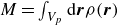 $M=\int _{V_{{p}}} {\rm d} \boldsymbol{r} \rho (\boldsymbol{r})$
is the total mass of the particle and
$M=\int _{V_{{p}}} {\rm d} \boldsymbol{r} \rho (\boldsymbol{r})$
is the total mass of the particle and $ V_{{p}}$
denotes the particle volume region. Similarly, the buoyancy forces are represented by a force acting at the centre of buoyancy
$ V_{{p}}$
denotes the particle volume region. Similarly, the buoyancy forces are represented by a force acting at the centre of buoyancy $\boldsymbol{R}_{{b}}$
, given by
$\boldsymbol{R}_{{b}}$
, given by
 \begin{equation} \boldsymbol{R}_{{b}} = \frac {1}{M_{{b}}} \int _{V_{{p}}} {\rm d}\boldsymbol{r} \rho _0 \boldsymbol{r}, \end{equation}
where $\rho _0$
is the density of the surrounding fluid and
$\rho _0$
is the density of the surrounding fluid and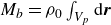 $M_{{b}}=\rho _0 \int _{V_{{p}}} {\rm d}\boldsymbol{r}$
is the total mass of the displaced fluid. Centres
$M_{{b}}=\rho _0 \int _{V_{{p}}} {\rm d}\boldsymbol{r}$
is the total mass of the displaced fluid. Centres $\boldsymbol{R}_{{m}}$
and
$\boldsymbol{R}_{{m}}$
and $\boldsymbol{R}_{{b}}$
must lie on the axis due to axisymmetry, but they are generally different because they depend on different mass distributions. Nevertheless, the two gravitational forces can be combined further. The total potential energy of the system is written as
$\boldsymbol{R}_{{b}}$
must lie on the axis due to axisymmetry, but they are generally different because they depend on different mass distributions. Nevertheless, the two gravitational forces can be combined further. The total potential energy of the system is written as
 \begin{equation} U= -\left (M \boldsymbol{g}\boldsymbol{\cdot }\boldsymbol{R}_{{m}} - M_{{b}} \boldsymbol{g} \boldsymbol{\cdot }\boldsymbol{R}_{{b}} \right ) = -(M-M_{{b}}) \boldsymbol{g}\boldsymbol{\cdot }\boldsymbol{R}_{{c}}. \end{equation}
Substituting (2.3) and (2.4) into (2.5), we can combine the effects of gravity and buoyancy acting on the particle, as shown in the second equality, which is equivalently represented by the force $(M-M_{{b}}) \boldsymbol{g}$
exerted on a point referred to as the sedimentation force centre (or simply the force centre). Even though
$(M-M_{{b}}) \boldsymbol{g}$
exerted on a point referred to as the sedimentation force centre (or simply the force centre). Even though $\boldsymbol{R}_{{m}}$
and
$\boldsymbol{R}_{{m}}$
and $\boldsymbol{R}_{{b}}$
are different, the position of the force centre is given by
$\boldsymbol{R}_{{b}}$
are different, the position of the force centre is given by
 \begin{equation} \boldsymbol{R}_{{c}} = \frac {1}{M-M_{{b}}} \int _{V_{{p}}} {\rm d}\boldsymbol{r} [\rho (\boldsymbol{r})-\rho _0] \boldsymbol{r}. \end{equation}
The force centre is defined only for particles with $M \neq M_{{b}}$
. In the following, we only consider such particles, since when
$M \neq M_{{b}}$
. In the following, we only consider such particles, since when $M=M_{{b}}$
, the particle does not sediment and therefore shows no Taylor dispersion.
$M=M_{{b}}$
, the particle does not sediment and therefore shows no Taylor dispersion.
The explicit expressions for the dispersion coefficients have been obtained for the case where the sedimentation force centre coincides with the hydrodynamic centre, $\boldsymbol{R}_{{c}} = \boldsymbol{R}_{{h}}$
. As illustrated in figure 1,
$\boldsymbol{R}_{{c}} = \boldsymbol{R}_{{h}}$
. As illustrated in figure 1, $\boldsymbol{R}_{{c}}$
generally differs from
$\boldsymbol{R}_{{c}}$
generally differs from $\boldsymbol{R}_{{h}}$
, because
$\boldsymbol{R}_{{h}}$
, because $\boldsymbol{R}_{{h}}$
is exclusively determined by surface geometry, whereas
$\boldsymbol{R}_{{h}}$
is exclusively determined by surface geometry, whereas $\boldsymbol{R}_{{c}}$
depends on the mass distribution within the particle. For an axisymmetric particle with
$\boldsymbol{R}_{{c}}$
depends on the mass distribution within the particle. For an axisymmetric particle with $\boldsymbol{R}_{{c}} \neq \boldsymbol{R}_{{h}}$
, one has
$\boldsymbol{R}_{{c}} \neq \boldsymbol{R}_{{h}}$
, one has
 \begin{equation} \boldsymbol{R}_{{c}}=\boldsymbol{R}_{{h}}+l_{{c}}\boldsymbol{n}, \end{equation}
since the two centres are on the same axis, where $l_{{c}}$
is the centre offset. One can also conduct the analyses with the separate offsets of the centres of mass
$l_{{c}}$
is the centre offset. One can also conduct the analyses with the separate offsets of the centres of mass $l_{{m}}$
and buoyancy
$l_{{m}}$
and buoyancy $l_{{b}}$
from
$l_{{b}}$
from $\boldsymbol{R}_{{h}}$
(defined by
$\boldsymbol{R}_{{h}}$
(defined by $\boldsymbol{R}_{{m}}=\boldsymbol{R}_{{h}}+l_{{m}}\boldsymbol{n}$
and
$\boldsymbol{R}_{{m}}=\boldsymbol{R}_{{h}}+l_{{m}}\boldsymbol{n}$
and $\boldsymbol{R}_{{b}}=\boldsymbol{R}_{{h}}+l_{{b}}\boldsymbol{n}$
). The offsets
$\boldsymbol{R}_{{b}}=\boldsymbol{R}_{{h}}+l_{{b}}\boldsymbol{n}$
). The offsets $l_{{m}}$
and
$l_{{m}}$
and $l_{{b}}$
are all rolled up into
$l_{{b}}$
are all rolled up into $l_{{c}}$
, which is expressed as
$l_{{c}}$
, which is expressed as
 \begin{equation} l_{{c}} = \frac {l_{{m}} M - l_{{b}} M_{{b}}}{M - M_{{b}}}. \end{equation}
Note that $l_{{c}}$
is zero even if
$l_{{c}}$
is zero even if $l_{{m}}$
and
$l_{{m}}$
and $l_{{b}}$
are non-zero when
$l_{{b}}$
are non-zero when $l_{{m}} M = l_{{b}} M_{{b}}$
. Adjustments to
$l_{{m}} M = l_{{b}} M_{{b}}$
. Adjustments to $l_{{c}}$
can be achieved by modifying either the particle’s asymmetric shape or its non-uniform mass distribution. While changes in shape also affect the friction coefficients, changes in mass distribution do not.
$l_{{c}}$
can be achieved by modifying either the particle’s asymmetric shape or its non-uniform mass distribution. While changes in shape also affect the friction coefficients, changes in mass distribution do not.
2.2. Smoluchowski equation under gravity
The configuration of the particle is entirely determined by independent variables $\boldsymbol{R}_{{h}}$
and
$\boldsymbol{R}_{{h}}$
and $\boldsymbol{n}$
. Due to the Brownian motion,
$\boldsymbol{n}$
. Due to the Brownian motion, $\boldsymbol{R}_{{h}}$
and
$\boldsymbol{R}_{{h}}$
and $\boldsymbol{n}$
evolve in a stochastic manner. Let
$\boldsymbol{n}$
evolve in a stochastic manner. Let $\psi ( \boldsymbol{R}_{{h}},\boldsymbol{n},t)$
denote the probability density function of finding the particle at position
$\psi ( \boldsymbol{R}_{{h}},\boldsymbol{n},t)$
denote the probability density function of finding the particle at position $\boldsymbol{R}_{{h}}$
and orientation
$\boldsymbol{R}_{{h}}$
and orientation $\boldsymbol{n}$
at time
$\boldsymbol{n}$
at time $t$
. The particle dynamics is governed by the hydrodynamic force (2.1) and gravitational force (gradient of (2.5)). Following Onsager’s variational principle (Appendix A), the probability density
$t$
. The particle dynamics is governed by the hydrodynamic force (2.1) and gravitational force (gradient of (2.5)). Following Onsager’s variational principle (Appendix A), the probability density $\psi$
evolves according to the Smoluchowski equation:
$\psi$
evolves according to the Smoluchowski equation:
 \begin{align} \frac {\partial \psi }{\partial t} &= D_{{r}} \frac {\partial }{\partial \boldsymbol{n}}\boldsymbol{\cdot }\left (\boldsymbol{\delta }-\boldsymbol{n}\boldsymbol{n}\right ) \boldsymbol{\cdot }\left (\frac {\partial \psi }{\partial \boldsymbol{n}} - \frac {(M-M_{{b}})l_{{c}}\boldsymbol{g}}{k_{{B}}\kern-1pt T}\psi \right ) \nonumber \\&\quad + D^\perp \frac {\partial }{\partial \boldsymbol{R}_{{h}}}\boldsymbol{\cdot }\left (\boldsymbol{\delta } + \frac {\zeta _{{t}}^\perp -\zeta _{{t}}^\parallel }{\zeta _{{t}}^\parallel } \boldsymbol{n}\boldsymbol{n}\right )\boldsymbol{\cdot }\left (\frac {\partial \psi }{\partial \boldsymbol{R}_{{h}}}-\frac {(M-M_{{b}})\boldsymbol{g}}{k_{{B}}\kern-1pt T}\psi \right )\!, \end{align}
where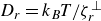 $D_{{r}} = k_{{B}}\kern-1pt T / \zeta _{{r}}^\perp$
is the rotational diffusion coefficient,
$D_{{r}} = k_{{B}}\kern-1pt T / \zeta _{{r}}^\perp$
is the rotational diffusion coefficient, $D^\perp = k_{{B}}\kern-1pt T / \zeta _{{t}}^\perp$
is the transverse diffusion coefficient,
$D^\perp = k_{{B}}\kern-1pt T / \zeta _{{t}}^\perp$
is the transverse diffusion coefficient, $k_{{B}}$
is the Boltzmann constant and
$k_{{B}}$
is the Boltzmann constant and $T$
is the temperature. We adopt the rotational relaxation time
$T$
is the temperature. We adopt the rotational relaxation time $\tau _{{r}}$
as the reference time scale:
$\tau _{{r}}$
as the reference time scale:
 \begin{equation} \tau _{{r}} = \frac {1}{D_{{r}}} = \frac {\zeta _{{r}}^\perp }{ k_{{B}}\kern-1pt T}. \end{equation}
The rotational relaxation time arises from the rotational diffusion in the absence of gravitational torque. It is the time scale beyond which correlations in the rod orientation become negligible. In the presence of gravity, the magnitude of the gravitational force and the maximum magnitude of the gravitational torque exerted on particles are given by $F_{{g}}=(M - M_{{b}})g$
and
$F_{{g}}=(M - M_{{b}})g$
and $T_{{g}}=(M - M_{{b}})gl_{{c}}$
, respectively, where
$T_{{g}}=(M - M_{{b}})gl_{{c}}$
, respectively, where $g=|\boldsymbol{g}|$
denotes the magnitude of the gravitational acceleration. The corresponding characteristic magnitudes of the translational velocity and angular velocities are
$g=|\boldsymbol{g}|$
denotes the magnitude of the gravitational acceleration. The corresponding characteristic magnitudes of the translational velocity and angular velocities are $u=F_{{g}}/\zeta _{{t}}^{\perp }$
and
$u=F_{{g}}/\zeta _{{t}}^{\perp }$
and $\omega =T_{{g}}/\zeta _{{r}}^{\perp }$
, respectively. Therefore, the system has two other characteristic time scales induced by gravitational effects. One is the reorientation time defined by
$\omega =T_{{g}}/\zeta _{{r}}^{\perp }$
, respectively. Therefore, the system has two other characteristic time scales induced by gravitational effects. One is the reorientation time defined by
 \begin{equation} \tau _{{o}} = \frac {1}{\omega } = \frac {\zeta _{{r}}^{\perp }}{ (M-M_{{b}})gl_{{c}} }, \end{equation}
which corresponds to the time scale associated with rotation caused by the gravitational torque in the absence of Brownian motion. The other is the sedimentation time, defined by
 \begin{equation} \tau _{{s}} = \frac {L}{u} = \frac {L\zeta _{{t}}^{\perp }}{ (M-M_{{b}}) g}, \end{equation}
where $L$
is the length scale of the particle, defined by its volume
$L$
is the length scale of the particle, defined by its volume $V$
as
$V$
as $L=[3V/(4\pi )]^{1/3}$
. It corresponds to the time scale for translation due to the gravitational force in the absence of Brownian motion. The ratios of rotational relaxation time to gravity-induced time scales,
$L=[3V/(4\pi )]^{1/3}$
. It corresponds to the time scale for translation due to the gravitational force in the absence of Brownian motion. The ratios of rotational relaxation time to gravity-induced time scales, $\tau _{{r}} / \tau _{{o}}$
and
$\tau _{{r}} / \tau _{{o}}$
and $\tau _{{r}} / \tau _{{s}}$
, are two key dimensionless parameters in this system. They are referred to as the reorientation Péclet number
$\tau _{{r}} / \tau _{{s}}$
, are two key dimensionless parameters in this system. They are referred to as the reorientation Péclet number $\alpha$
(also referred to as the dimensionless Langevin parameter in Brenner (Reference Brenner1979)) and the sedimentation Péclet number
$\alpha$
(also referred to as the dimensionless Langevin parameter in Brenner (Reference Brenner1979)) and the sedimentation Péclet number $\beta$
, respectively:
$\beta$
, respectively:
 \begin{equation} \alpha = \frac {\tau _{{r}}}{\tau _{{o}}} =\frac { (M-M_{{b}})gl_{{c}}}{ k_{{B}}\kern-1pt T}, \qquad \beta = \frac {\tau _{{r}}}{\tau _{{s}}} = \frac {\zeta _{{r}}^{\perp }}{\zeta _{{t}}^{\perp }} \frac {(M-M_{{b}}) g}{L k_{{B}}\kern-1pt T}. \end{equation}
For a very large $\alpha$
, the gravitational torque overwhelms rotational Brownian fluctuations, and particle rotation is dominated by gravitational torque rather than rotational diffusion. Similarly, for a very large
$\alpha$
, the gravitational torque overwhelms rotational Brownian fluctuations, and particle rotation is dominated by gravitational torque rather than rotational diffusion. Similarly, for a very large $\beta$
, particle translation is dominated by gravitational force.
$\beta$
, particle translation is dominated by gravitational force.
We adopt $\tau _{{r}}$
and
$\tau _{{r}}$
and $L$
as the unit of time and length. Introducing dimensionless time
$L$
as the unit of time and length. Introducing dimensionless time $\tilde {t} = t / \tau _{{r}}$
and position
$\tilde {t} = t / \tau _{{r}}$
and position $ \tilde {\boldsymbol{R}}_{{h}} = \boldsymbol{R}_{{h}} / L$
, the Smoluchowski equation (2.9) is non-dimensionalised to
$ \tilde {\boldsymbol{R}}_{{h}} = \boldsymbol{R}_{{h}} / L$
, the Smoluchowski equation (2.9) is non-dimensionalised to
 \begin{equation} \frac {\partial \psi }{\partial \tilde {t}} = \tilde {\mathcal{L}}\psi , \end{equation}
with
 \begin{equation} \tilde {\mathcal{L}} = \frac {\partial }{\partial \boldsymbol{n}}\boldsymbol{\cdot }\left (\boldsymbol{\delta }-\boldsymbol{n}\boldsymbol{n}\right )\boldsymbol{\cdot }\left (\frac {\partial }{\partial \boldsymbol{n}} - \alpha \hat {\boldsymbol{g}}\right ) + \frac {\partial }{\partial \tilde {\boldsymbol{R}}_{{h}}}\boldsymbol{\cdot }\left (\boldsymbol{\delta }+\chi \boldsymbol{n}\boldsymbol{n}\right )\boldsymbol{\cdot }\left (\tilde {D}^\perp \frac {\partial }{\partial \tilde {\boldsymbol{R}}_{{h}}}-\beta \hat {\boldsymbol{g}}\right )\!, \end{equation}
where $\hat {\boldsymbol{g}} = \boldsymbol{g} /g$
, and we have defined
$\hat {\boldsymbol{g}} = \boldsymbol{g} /g$
, and we have defined
 \begin{equation} \chi = \frac {\zeta _{{t}}^\perp -\zeta _{{t}}^\parallel }{ \zeta _{{t}}^\parallel }, \end{equation}
which characterises the hydrodynamic anisotropy of the particle. The dimensionless transverse diffusion coefficient $\tilde {D}^\perp$
is given by
$\tilde {D}^\perp$
is given by
 \begin{equation} \tilde {D}^\perp = \frac {D^\perp \tau _{{r}}}{L^2} = \frac {\zeta _{{r}}^\perp }{\zeta _{{t}}^\perp L^2} . \end{equation}
Using the results in Appendix D, the dimensionless friction-related quantities $\chi$
and
$\chi$
and $\tilde {D}^\perp$
depend solely on the aspect ratio
$\tilde {D}^\perp$
depend solely on the aspect ratio $r$
.
$r$
.
Let $\tilde {\varOmega }=(\tilde {\boldsymbol{R}}_{{h}},\boldsymbol{n})$
denotes the particle configuration at time
$\tilde {\varOmega }=(\tilde {\boldsymbol{R}}_{{h}},\boldsymbol{n})$
denotes the particle configuration at time $\tilde {t}$
and
$\tilde {t}$
and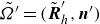 $\tilde {\varOmega }^\prime=(\tilde {\boldsymbol{R}}_{{h}}^\prime,\boldsymbol{n}^\prime)$
denotes the configuration at
$\tilde {\varOmega }^\prime=(\tilde {\boldsymbol{R}}_{{h}}^\prime,\boldsymbol{n}^\prime)$
denotes the configuration at $\tilde {t}^\prime$
. Given the initial condition
$\tilde {t}^\prime$
. Given the initial condition $\left .\psi \right |_{\tilde {t}=\tilde {t}^\prime}=\delta (\tilde {\boldsymbol{R}}_{{h}}-\tilde {\boldsymbol{R}}_{{h}}^\prime)\delta (\boldsymbol{n}-\boldsymbol{n}^\prime)$
, the solution of the Smoluchowski equation (2.14) is the Green’s function, which is denoted by
$\left .\psi \right |_{\tilde {t}=\tilde {t}^\prime}=\delta (\tilde {\boldsymbol{R}}_{{h}}-\tilde {\boldsymbol{R}}_{{h}}^\prime)\delta (\boldsymbol{n}-\boldsymbol{n}^\prime)$
, the solution of the Smoluchowski equation (2.14) is the Green’s function, which is denoted by $\mathcal{G}(\tilde {\varOmega },\tilde {t};\tilde {\varOmega }^\prime,\tilde {t}^\prime)$
. The Green’s function represents the conditional probability density of finding the particle in
$\mathcal{G}(\tilde {\varOmega },\tilde {t};\tilde {\varOmega }^\prime,\tilde {t}^\prime)$
. The Green’s function represents the conditional probability density of finding the particle in $\tilde {\varOmega }$
at time
$\tilde {\varOmega }$
at time $\tilde {t}$
, given that it was in
$\tilde {t}$
, given that it was in $\tilde {\varOmega }^\prime$
at
$\tilde {\varOmega }^\prime$
at $\tilde {t}^\prime$
. Therefore, the ensemble average of a quantity
$\tilde {t}^\prime$
. Therefore, the ensemble average of a quantity $\boldsymbol{\mathcal{F}}(\tilde {\varOmega },\tilde {\varOmega }^\prime)$
can be generally obtained using the Green’s function and initial distribution
$\boldsymbol{\mathcal{F}}(\tilde {\varOmega },\tilde {\varOmega }^\prime)$
can be generally obtained using the Green’s function and initial distribution $\psi _{\textit{in}}$
at
$\psi _{\textit{in}}$
at $\tilde {t}^\prime$
, i.e.
$\tilde {t}^\prime$
, i.e.
 \begin{equation} \left\langle \boldsymbol{\mathcal{F}}\left(\tilde {t},\tilde {t}^\prime\right)\right\rangle = \int {\rm d}\tilde {\varOmega } \int {\rm d}\tilde {\varOmega }^\prime\mathcal{G}\left(\tilde {\varOmega },\tilde {t};\tilde {\varOmega }^\prime,\tilde {t}^\prime\right)\psi _{\textit{in}}\left(\tilde {\varOmega }^\prime,\tilde {t}^\prime\right)\boldsymbol{\mathcal{F}}\left(\tilde {\varOmega },\tilde {\varOmega }^\prime\right)\!, \end{equation}
where ${\rm d}\tilde {\varOmega }^\prime={\rm d}\tilde {\boldsymbol{R}}_{{h}}^\prime {\rm d}\boldsymbol{n}^\prime$
is the volume element in the dimensionless configuration space
${\rm d}\tilde {\varOmega }^\prime={\rm d}\tilde {\boldsymbol{R}}_{{h}}^\prime {\rm d}\boldsymbol{n}^\prime$
is the volume element in the dimensionless configuration space $\tilde {\varOmega }^\prime $
.
$\tilde {\varOmega }^\prime $
.
Additionally, one can multiply both sides of the Smoluchowski equation (2.14a
) by the function $\boldsymbol{\mathcal{F}}(\tilde {\boldsymbol{R}}_{{h}},\boldsymbol{n},\tilde {\boldsymbol{R}}_{{h}}^\prime,\boldsymbol{n}^\prime)$
and use the definition of the Green’s function to obtain the following evolution equation (Doi & Edwards Reference Doi and Edwards1986; Xiong, Seto & Doi Reference Xiong, Seto and Doi2024):
$\boldsymbol{\mathcal{F}}(\tilde {\boldsymbol{R}}_{{h}},\boldsymbol{n},\tilde {\boldsymbol{R}}_{{h}}^\prime,\boldsymbol{n}^\prime)$
and use the definition of the Green’s function to obtain the following evolution equation (Doi & Edwards Reference Doi and Edwards1986; Xiong, Seto & Doi Reference Xiong, Seto and Doi2024):
 \begin{equation} \frac {\partial \left\langle \boldsymbol{\mathcal{F}}\left(\tilde {t},\tilde {t}^\prime\right)\right\rangle }{\partial \tilde {t}} = \left\langle \tilde {\mathcal{L}}^\dagger \boldsymbol{\mathcal{F}}\left(\tilde {\boldsymbol{R}}_{{h}},\boldsymbol{n},\tilde {\boldsymbol{R}}_{{h}}^\prime,\boldsymbol{n}^\prime\right)\right\rangle\! , \end{equation}
where $\tilde {\mathcal{L}}^\dagger$
is the conjugate operator of
$\tilde {\mathcal{L}}^\dagger$
is the conjugate operator of $\tilde {\mathcal{L}}$
defined by
$\tilde {\mathcal{L}}$
defined by
 \begin{equation} \tilde {\mathcal{L}}^\dagger = \left (\frac {\partial }{\partial \boldsymbol{n}} + \alpha \hat {\boldsymbol{g}}\right )\boldsymbol{\cdot }\left (\boldsymbol{\delta }-\boldsymbol{n}\boldsymbol{n}\right )\boldsymbol{\cdot }\frac {\partial }{\partial \boldsymbol{n}} + \left (\tilde {D}^\perp \frac {\partial }{\partial \tilde {\boldsymbol{R}}_{{h}}} + \beta \hat {\boldsymbol{g}}\right )\boldsymbol{\cdot }\left (\boldsymbol{\delta }+\chi \boldsymbol{n}\boldsymbol{n}\right ) \boldsymbol{\cdot }\frac {\partial }{\partial \tilde {\boldsymbol{R}}_{{h}}}. \end{equation}
The ensemble average could also be calculated via (2.18) without explicitly knowing the Green’s function.
3. Sedimentation and dispersion
3.1. Application of the Smoluchowski equation
We now examine the sedimentation behaviour of such a particle in a gravitational field. Here, we set the gravity direction as $\hat {\boldsymbol{g}}=-\boldsymbol{e}_z$
and consider the sedimentation process starting from the origin,
$\hat {\boldsymbol{g}}=-\boldsymbol{e}_z$
and consider the sedimentation process starting from the origin, $\tilde {\boldsymbol{R}}_{{h}}(0)=\boldsymbol{0}$
. The unit basis vectors along the
$\tilde {\boldsymbol{R}}_{{h}}(0)=\boldsymbol{0}$
. The unit basis vectors along the $x$
,
$x$
, $y$
and
$y$
and $z$
axes are denoted by
$z$
axes are denoted by $\boldsymbol{e}_x$
,
$\boldsymbol{e}_x$
, $\boldsymbol{e}_y$
and
$\boldsymbol{e}_y$
and $\boldsymbol{e}_z$
, respectively. Since the anisotropy in this system arises solely from gravity, the sedimentation process with horizontal motion can be statistically characterised by the mean position coordinate along the gravity direction
$\boldsymbol{e}_z$
, respectively. Since the anisotropy in this system arises solely from gravity, the sedimentation process with horizontal motion can be statistically characterised by the mean position coordinate along the gravity direction $\langle \tilde {z}_{{h}}(\tilde {t}) \rangle$
, and the MSD in the
$\langle \tilde {z}_{{h}}(\tilde {t}) \rangle$
, and the MSD in the $x$
–
$x$
– $y$
plane
$y$
plane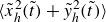 $\langle \tilde {x}_{{h}}^2(\tilde {t}) + \tilde {y}_{{h}}^2(\tilde {t})\rangle$
. They are expressed as follows:
$\langle \tilde {x}_{{h}}^2(\tilde {t}) + \tilde {y}_{{h}}^2(\tilde {t})\rangle$
. They are expressed as follows:
 \begin{align}&\quad \tilde {z}_{{h}}\big(\tilde {t}\big) =\boldsymbol{e}_z\boldsymbol{\cdot }\tilde {\boldsymbol{R}}_{{h}}\big(\tilde {t}\big)= -\hat {\boldsymbol{g}}\boldsymbol{\cdot }\left[\tilde {\boldsymbol{R}}_{{h}}\big(\tilde {t}\big)-\tilde {\boldsymbol{R}}_{{h}}(0)\right]\!, \end{align}
 \begin{align}& \tilde {x}_{{h}}^2\big(\tilde {t}\big)+\tilde {y}_{{h}}^2\big(\tilde {t}\big) = \left \{\big(\boldsymbol{\delta }-\hat {\boldsymbol{g}}\hat {\boldsymbol{g}}\big)\boldsymbol{\cdot }\left[\tilde {\boldsymbol{R}}_{{h}}\big(\tilde {t}\big)-\tilde {\boldsymbol{R}}_{{h}}(0)\right] \right \}^2. \end{align}
The mean position $\langle \tilde {z}_{{h}}(\tilde {t})\rangle$
(the drift displacement in the
$\langle \tilde {z}_{{h}}(\tilde {t})\rangle$
(the drift displacement in the $z$
direction) during sedimentation is obtained by applying (2.18a
) to (3.1a
), yielding
$z$
direction) during sedimentation is obtained by applying (2.18a
) to (3.1a
), yielding
 \begin{gather} \frac {\partial \langle \tilde {z}_{{h}}\rangle }{\partial \tilde {t}} = -\left \langle \tilde {\mathcal{L}}^\dagger \hat {\boldsymbol{g}}\boldsymbol{\cdot }\left[\tilde {\boldsymbol{R}}_{{h}}\bigl(\tilde {t}\bigr)-\tilde {\boldsymbol{R}}_{{h}}(0)\right] \right \rangle = -\beta \big ( 1+\chi \hat {\boldsymbol{g}}\boldsymbol{\cdot }\left \langle \boldsymbol{n}\boldsymbol{n} \right \rangle \boldsymbol{\cdot }\hat {\boldsymbol{g}} \big ). \end{gather}
Similarly, applying (2.18a ) to the square of (3.1a ) yields (see Appendix C for details)
 \begin{align} \frac {\partial \left\langle \left [\tilde {z}_{{h}}-\langle \tilde {z}_{{h}}\rangle \right ]^2\right\rangle }{\partial \tilde {t}} &= 2\tilde {D}^\perp \big ( 1+\chi \hat {\boldsymbol{g}}\boldsymbol{\cdot }\left \langle \boldsymbol{n}\boldsymbol{n} \right \rangle \boldsymbol{\cdot }\hat {\boldsymbol{g}} \big ) \notag \\ &\quad +2\left (\beta \chi \right )^2\int _0^{\tilde {t}}{\rm d}\tilde {t}^\prime\left [\left \langle \hat {\boldsymbol{g}}\boldsymbol{\cdot }\boldsymbol{n}\boldsymbol{n}\boldsymbol{\cdot }\hat {\boldsymbol{g}}\hat {\boldsymbol{g}}\boldsymbol{\cdot }\boldsymbol{n}^\prime\boldsymbol{n}^\prime \boldsymbol{\cdot }\hat {\boldsymbol{g}}\right \rangle -\hat {\boldsymbol{g}}\boldsymbol{\cdot }\left \langle \boldsymbol{n}\boldsymbol{n}\right \rangle \boldsymbol{\cdot }\hat {\boldsymbol{g}}\hat {\boldsymbol{g}}\boldsymbol{\cdot }\left \langle \boldsymbol{n}^\prime\boldsymbol{n}^\prime \right \rangle \boldsymbol{\cdot }\hat {\boldsymbol{g}}\right ]\!, \end{align}
where $ \langle [\tilde {z}_{{h}}-\langle \tilde {z}_{{h}}\rangle ]^2\rangle$
represents the
$ \langle [\tilde {z}_{{h}}-\langle \tilde {z}_{{h}}\rangle ]^2\rangle$
represents the $z$
-direction MSD with eliminating the drift displacement in the
$z$
-direction MSD with eliminating the drift displacement in the $z$
direction. Here
$z$
direction. Here $\boldsymbol{n}$
and
$\boldsymbol{n}$
and $\boldsymbol{n}^\prime$
denote the orientation of the particle at time
$\boldsymbol{n}^\prime$
denote the orientation of the particle at time $\tilde {t}$
and
$\tilde {t}$
and $\tilde {t}^\prime$
, respectively. The MSD in the
$\tilde {t}^\prime$
, respectively. The MSD in the $x$
–
$x$
– $y$
plane is obtained by applying (2.18a
) to (3.1b
), yielding
$y$
plane is obtained by applying (2.18a
) to (3.1b
), yielding
 \begin{align} \frac {\partial \left \langle \tilde {x}_{{h}}^2+\tilde {y}_{{h}}^2 \right \rangle }{\partial \tilde {t}} &= 2\tilde {D}^\perp \left [2+\chi \big (1- \hat {\boldsymbol{g}}\boldsymbol{\cdot }\left \langle \boldsymbol{n}\boldsymbol{n} \right \rangle \boldsymbol{\cdot }\hat {\boldsymbol{g}} \big )\right ] \notag \\ &\quad +2\left (\beta \chi \right )^2\int _0^{\tilde {t}}{\rm d}\tilde {t}^\prime\left \langle \hat {\boldsymbol{g}}\boldsymbol{\cdot }\boldsymbol{n}\boldsymbol{n}\boldsymbol{\cdot }(\boldsymbol{\delta }-\hat {\boldsymbol{g}}\hat {\boldsymbol{g}})\boldsymbol{\cdot }\boldsymbol{n}^\prime\boldsymbol{n}^\prime\boldsymbol{\cdot }\hat {\boldsymbol{g}}\right \rangle . \end{align}
3.2. Orientational distribution under gravitational torque
Note that calculation of the sedimentation velocity (from (3.2)) and diffusion (from (3.3) and (3.4)) requires first evaluating the orientation dynamics, especially calculating quantities such as $\left \langle \boldsymbol{n}\boldsymbol{n} \right \rangle$
,
$\left \langle \boldsymbol{n}\boldsymbol{n} \right \rangle$
, $\left \langle \hat {\boldsymbol{g}}\boldsymbol{\cdot }\boldsymbol{n}\boldsymbol{n}\boldsymbol{\cdot }\hat {\boldsymbol{g}}\hat {\boldsymbol{g}}\boldsymbol{\cdot }\boldsymbol{n}^\prime\boldsymbol{n}^\prime \boldsymbol{\cdot }\hat {\boldsymbol{g}}\right \rangle$
and
$\left \langle \hat {\boldsymbol{g}}\boldsymbol{\cdot }\boldsymbol{n}\boldsymbol{n}\boldsymbol{\cdot }\hat {\boldsymbol{g}}\hat {\boldsymbol{g}}\boldsymbol{\cdot }\boldsymbol{n}^\prime\boldsymbol{n}^\prime \boldsymbol{\cdot }\hat {\boldsymbol{g}}\right \rangle$
and $\left \langle \hat {\boldsymbol{g}}\boldsymbol{\cdot }\boldsymbol{n}\boldsymbol{n}\boldsymbol{\cdot }(\boldsymbol{\delta }-\hat {\boldsymbol{g}}\hat {\boldsymbol{g}})\boldsymbol{\cdot }\boldsymbol{n}^\prime\boldsymbol{n}^\prime\boldsymbol{\cdot }\hat {\boldsymbol{g}}\right \rangle$
. Since these ensemble averages depend solely on orientation, integration over
$\left \langle \hat {\boldsymbol{g}}\boldsymbol{\cdot }\boldsymbol{n}\boldsymbol{n}\boldsymbol{\cdot }(\boldsymbol{\delta }-\hat {\boldsymbol{g}}\hat {\boldsymbol{g}})\boldsymbol{\cdot }\boldsymbol{n}^\prime\boldsymbol{n}^\prime\boldsymbol{\cdot }\hat {\boldsymbol{g}}\right \rangle$
. Since these ensemble averages depend solely on orientation, integration over $\tilde {\boldsymbol{R}}_{{h}}$
can be performed directly. Defining the probability distribution of the orientation by
$\tilde {\boldsymbol{R}}_{{h}}$
can be performed directly. Defining the probability distribution of the orientation by
 \begin{equation} \psi (\boldsymbol{n},\tilde {t})=\int {\rm d}\tilde {\boldsymbol{R}}_{{h}} \psi \left( \tilde {\boldsymbol{R}}_{{h}},\boldsymbol{n},\tilde {t}\right)\!, \end{equation}
with ${\rm d}\tilde {\boldsymbol{R}}_{{h}} = {\rm d}\tilde {x}_{{h}} {\rm d}\tilde {y}_{{h}} {\rm d}\tilde {z}_{{h}}$
, the integration of (2.17) gives
${\rm d}\tilde {\boldsymbol{R}}_{{h}} = {\rm d}\tilde {x}_{{h}} {\rm d}\tilde {y}_{{h}} {\rm d}\tilde {z}_{{h}}$
, the integration of (2.17) gives
 \begin{equation} \left\langle \boldsymbol{\mathcal{F}}\big(\tilde {t}\big)\right\rangle = \int {\rm d}\tilde {\varOmega } \psi \left(\tilde {\boldsymbol{R}}_{{h}},\boldsymbol{n},\tilde {t}\right)\boldsymbol{\mathcal{F}}(\boldsymbol{n}) = \int {\rm d}\boldsymbol{n} \psi \left(\boldsymbol{n},\tilde {t}\right)\boldsymbol{\mathcal{F}}(\boldsymbol{n}). \end{equation}
The orientation vector $\boldsymbol{n}$
is expressed in spherical coordinates as
$\boldsymbol{n}$
is expressed in spherical coordinates as $\boldsymbol{n}=\sin \theta \cos \phi \boldsymbol{e}_x +\sin \theta \sin \phi \boldsymbol{e}_y +\cos \theta \boldsymbol{e}_z$
with
$\boldsymbol{n}=\sin \theta \cos \phi \boldsymbol{e}_x +\sin \theta \sin \phi \boldsymbol{e}_y +\cos \theta \boldsymbol{e}_z$
with $\theta \in [0,\pi ]$
and
$\theta \in [0,\pi ]$
and $\phi \in [0,2\pi ]$
, illustrated in figure 1. Then the orientational distribution is expressed as
$\phi \in [0,2\pi ]$
, illustrated in figure 1. Then the orientational distribution is expressed as $\psi (\boldsymbol{n},\tilde {t})=\psi (\theta ,\phi ,\tilde {t})$
, and
$\psi (\boldsymbol{n},\tilde {t})=\psi (\theta ,\phi ,\tilde {t})$
, and ${\rm d}\boldsymbol{n}=\sin \theta {\rm d}\theta {\rm d}\phi$
. The equation governing
${\rm d}\boldsymbol{n}=\sin \theta {\rm d}\theta {\rm d}\phi$
. The equation governing $\psi (\theta ,\phi ,\tilde {t})$
is obtained by integrating both sides of (2.14a
) over
$\psi (\theta ,\phi ,\tilde {t})$
is obtained by integrating both sides of (2.14a
) over $\tilde {\boldsymbol{R}}_{{h}}$
, which reads
$\tilde {\boldsymbol{R}}_{{h}}$
, which reads
 \begin{equation} \frac {\partial \psi }{\partial \tilde {t}}=\tilde {\mathcal{L}}_{{sp}}\psi = \frac {1}{\sin \theta }\frac {\partial }{\partial \theta }\left (\sin \theta \frac {\partial \psi }{\partial \theta }\right )+\frac {1}{\sin ^2\theta }\frac {\partial ^2\psi }{\partial \phi ^2}-\alpha \left (\sin \theta \frac {\partial \psi }{\partial \theta }+2\cos \theta \psi \right )\!, \end{equation}
with the periodic boundary condition $\left .\psi \right |_{\phi =0}=\left .\psi \right |_{\phi =2\pi }$
and boundedness conditions of
$\left .\psi \right |_{\phi =0}=\left .\psi \right |_{\phi =2\pi }$
and boundedness conditions of $\psi$
at
$\psi$
at $\theta =0,\pi$
. The normalisation condition is
$\theta =0,\pi$
. The normalisation condition is $\int _0^{2\pi }{\rm d}\phi \int _0^\pi {\rm d}\theta \sin \theta \psi =1$
. The steady-state orientation distribution can be obtained analytically by solving
$\int _0^{2\pi }{\rm d}\phi \int _0^\pi {\rm d}\theta \sin \theta \psi =1$
. The steady-state orientation distribution can be obtained analytically by solving $\tilde {\mathcal{L}}_{{sp}} \psi _{\textit{ss}} = 0$
, and the solution is
$\tilde {\mathcal{L}}_{{sp}} \psi _{\textit{ss}} = 0$
, and the solution is
 \begin{equation} \psi _{\textit{ss}}(\theta ,\phi ) = \frac {\alpha }{4\pi \sinh \alpha }{\rm e}^{-\alpha \cos \theta } \end{equation}
(see also Brenner Reference Brenner1979; Dill & Brenner Reference Dill and Brenner1983). Figure 2 illustrates the distribution. The orientational distribution of a sedimenting particle in a steady-state is the same as the equilibrium distribution of a particle whose hydrodynamic centre is fixed in space. Due to the rotational symmetry about the $\hat {\boldsymbol{g}}$
direction, the steady-state orientation distribution is independent of
$\hat {\boldsymbol{g}}$
direction, the steady-state orientation distribution is independent of $\phi$
. When the hydrodynamic centre coincides with the force centre (
$\phi$
. When the hydrodynamic centre coincides with the force centre ( $l_{{c}}=0$
),
$l_{{c}}=0$
), $\alpha$
becomes equal to zero, and (3.8) reduces to the uniform distribution
$\alpha$
becomes equal to zero, and (3.8) reduces to the uniform distribution $\psi _{\textit{ss}}(\theta ,\phi ) = 1/(4\pi )$
(Frankel Reference Frankel1991), which represents a uniform distribution over a unit spherical surface.
$\psi _{\textit{ss}}(\theta ,\phi ) = 1/(4\pi )$
(Frankel Reference Frankel1991), which represents a uniform distribution over a unit spherical surface.
Steady-state orientation probability distribution $\psi _{\textit{ss}}(\theta , \phi )$
for an axisymmetric Brownian particle. Inset: the distribution weighted by
$\psi _{\textit{ss}}(\theta , \phi )$
for an axisymmetric Brownian particle. Inset: the distribution weighted by $\sin \theta$
, accounting for the spherical area element associated with polar angle
$\sin \theta$
, accounting for the spherical area element associated with polar angle $\theta$
.
$\theta$
.

Figure 2. Long description
A line graph showing the steady-state orientation probability distribution for an axisymmetric Brownian particle. The main graph displays three lines representing different values of \alpha, with the x-axis labeled as theta ranging from 0 to pi and the y-axis labeled as psi subscript ss ranging from 0 to 0.3. The inset graph shows the distribution weighted by psi subscript ss sine theta, with the x-axis labeled as theta ranging from 0 to pi and the y-axis labeled as psi subscript ss sine theta ranging from 0 to 0.3. The lines in the main graph are color-coded: red for 1, blue for 2, and green for 10. The inset graph also features three lines corresponding to the same values. All values are approximated.
Using the steady-state distribution $\psi _{\textit{ss}}$
, the original (3.7) can be solved via the Green’s function
$\psi _{\textit{ss}}$
, the original (3.7) can be solved via the Green’s function $\mathcal{G}$
, determined through an eigenfunction expansion:
$\mathcal{G}$
, determined through an eigenfunction expansion:
 \begin{gather} \mathcal{G}(\theta ,\phi ,\tilde {t};\theta ^\prime,\phi ^\prime) = \psi _{\textit{ss}}^{-1}(\theta ^\prime,\phi ^\prime)\sum _{p=0}^\infty \psi _p(\theta ,\phi )\psi _p(\theta ^\prime,\phi ^\prime){\rm e}^{-\lambda _p\tilde {t}}, \end{gather}
where $\lambda _p$
and
$\lambda _p$
and $\psi _p$
(
$\psi _p$
( $p=0,1,2, \dotsc$
) are the eigenvalues and the eigenfunctions of the torque-dependent eigenvalue equation
$p=0,1,2, \dotsc$
) are the eigenvalues and the eigenfunctions of the torque-dependent eigenvalue equation
 \begin{equation} \tilde {\mathcal{L}}_{{sp}}\psi _p=-\lambda _p\psi _p. \end{equation}
The eigenfunctions satisfy the orthonormality condition $\int _0^{2\pi }{\rm d}\phi \int _0^\pi {\rm d}\theta \sin \theta \psi _{\textit{ss}}^{-1}\psi _p\psi _q=\delta _{p,q}$
with weight
$\int _0^{2\pi }{\rm d}\phi \int _0^\pi {\rm d}\theta \sin \theta \psi _{\textit{ss}}^{-1}\psi _p\psi _q=\delta _{p,q}$
with weight $\psi _{\textit{ss}}^{-1}$
. It can generally be proved that the eigenvalues
$\psi _{\textit{ss}}^{-1}$
. It can generally be proved that the eigenvalues $\lambda _p$
are all non-negative and real (Doi & Edwards Reference Doi and Edwards1986). The sole zero eigenvalue
$\lambda _p$
are all non-negative and real (Doi & Edwards Reference Doi and Edwards1986). The sole zero eigenvalue $\lambda _0=0$
is included in (3.9), indicating that
$\lambda _0=0$
is included in (3.9), indicating that $\psi (\theta ,\phi ,\tilde {t})$
ultimately converges to the steady-state distribution
$\psi (\theta ,\phi ,\tilde {t})$
ultimately converges to the steady-state distribution $\psi _0=\psi _{\textit{ss}}(\theta ,\phi )$
over time. Other eigenfunctions
$\psi _0=\psi _{\textit{ss}}(\theta ,\phi )$
over time. Other eigenfunctions $\psi _p$
(
$\psi _p$
( $p=1,2,3,\dotsc$
) are obtained numerically (see Appendix C), and they satisfy
$p=1,2,3,\dotsc$
) are obtained numerically (see Appendix C), and they satisfy $\int _0^{2\pi }{\rm d}\phi \int _0^\pi {\rm d}\theta \sin \theta \psi _p=0$
for
$\int _0^{2\pi }{\rm d}\phi \int _0^\pi {\rm d}\theta \sin \theta \psi _p=0$
for $p=1,2,3,\dotsc$
from the orthonormality. Therefore, using the Green’s function and the initial distribution of orientation
$p=1,2,3,\dotsc$
from the orthonormality. Therefore, using the Green’s function and the initial distribution of orientation $\psi _{\textit{in}}$
, the solution of (3.7) is
$\psi _{\textit{in}}$
, the solution of (3.7) is
 \begin{align} \psi (\theta ,\phi ,\tilde {t}) &= \int _0^{2\pi }{\rm d}\phi ^\prime\int _0^\pi {\rm d}\theta ^\prime\sin \theta ^\prime\mathcal{G}(\theta ,\phi ,\tilde {t};\theta ^\prime,\phi ^\prime)\psi _{\textit{in}}(\theta ^\prime,\phi ^\prime) \notag \\ &= \psi _{\textit{ss}}(\theta ,\phi ) + \sum _{p=1}^\infty c_p \psi _p(\theta ,\phi ){\rm e}^{-\lambda _p\tilde {t}}, \end{align}
where $c_p = \int _0^{2\pi }{\rm d}\phi ^\prime\int _0^\pi {\rm d}\theta ^\prime\sin \theta ^\prime\psi _{\textit{ss}}^{-1}(\theta ^\prime,\phi ^\prime)\psi _{\textit{in}}(\theta ^\prime,\phi ^\prime)\psi _p(\theta ^\prime,\phi ^\prime)$
.
$c_p = \int _0^{2\pi }{\rm d}\phi ^\prime\int _0^\pi {\rm d}\theta ^\prime\sin \theta ^\prime\psi _{\textit{ss}}^{-1}(\theta ^\prime,\phi ^\prime)\psi _{\textit{in}}(\theta ^\prime,\phi ^\prime)\psi _p(\theta ^\prime,\phi ^\prime)$
.
For example, ensemble averages $\langle n_z\rangle$
and
$\langle n_z\rangle$
and $\langle n_z^2\rangle$
are calculated using the solution (3.11). The long-time behaviour can generally be obtained from the steady-state distribution function (3.8) as
$\langle n_z^2\rangle$
are calculated using the solution (3.11). The long-time behaviour can generally be obtained from the steady-state distribution function (3.8) as
 \begin{align} \lim _{\tilde {t} \to \infty } \langle n_z\big(\tilde {t}\big)\rangle &= \langle n_z\rangle _{\textit{ss}} = \int _0^{2\pi }{\rm d}\phi \int _0^\pi {\rm d}\theta \sin \theta \psi _{\textit{ss}}(\theta ,\phi )\cos \theta =-\frac {\alpha \coth \alpha -1}{\alpha }, \end{align}
 \begin{align} \lim _{\tilde {t} \to \infty } \langle n_z^2\big(\tilde {t}\big)\rangle &= \langle n_z^2\rangle _{\textit{ss}} = \int _0^{2\pi }{\rm d}\phi \int _0^\pi {\rm d}\theta \sin \theta \psi _{\textit{ss}}(\theta ,\phi )\cos ^2\theta =1-2\frac {\alpha \coth \alpha -1}{\alpha ^2}. \end{align}
It shows that the particle develops a preferred orientation along the direction of gravity when gravitational torque exists. Similarly, the steady-state ensemble average $\langle \boldsymbol{n}\boldsymbol{n}\rangle _{\textit{ss}}$
is obtained by
$\langle \boldsymbol{n}\boldsymbol{n}\rangle _{\textit{ss}}$
is obtained by
 \begin{equation} \langle \boldsymbol{n}\boldsymbol{n}\rangle _{\textit{ss}} = \frac {1}{3}\boldsymbol{\delta }+\left (1-3\frac {\alpha \coth \alpha -1}{\alpha ^2}\right )\left (\hat {\boldsymbol{g}}\hat {\boldsymbol{g}}-\frac {1}{3}\boldsymbol{\delta }\right )\!. \end{equation}
The transient behaviour before the system reaches the steady-state can also be calculated numerically via eigenfunction expansion of the Green’s function (3.9), or analytically via perturbation expansion for the moment $\langle (\hat {\boldsymbol{g}} \boldsymbol{\cdot }\boldsymbol{n})^2\rangle$
with respect to
$\langle (\hat {\boldsymbol{g}} \boldsymbol{\cdot }\boldsymbol{n})^2\rangle$
with respect to $\alpha$
(see (B1a
)).
$\alpha$
(see (B1a
)).
For small $\alpha$
, the latter method yields the following expression for
$\alpha$
, the latter method yields the following expression for $\langle n_z(\tilde {t})\rangle$
for a particle which is distributed isotropically at
$\langle n_z(\tilde {t})\rangle$
for a particle which is distributed isotropically at $\tilde t =0$
:
$\tilde t =0$
:
 \begin{align} \left\langle n_z\big(\tilde {t}\big)\right\rangle &= \boldsymbol{e}_z\boldsymbol{\cdot }\left\langle \boldsymbol{n}\big(\tilde {t}\big)\right\rangle = -\frac {\alpha }{3} \left (1-{\rm e}^{-2\tilde {t}} \right )+o\big(\alpha ^2\big). \end{align}
Equation (3.14) approaches the asymptotic value given by (3.12a
) as $\tilde {t} \to \infty$
.
$\tilde {t} \to \infty$
.
For large $\alpha$
, the gravitational torque overwhelms rotational Brownian fluctuations, locking the particle into a nearly fixed orientation. If the particle is nearly in a gravity-aligned configuration, one has
$\alpha$
, the gravitational torque overwhelms rotational Brownian fluctuations, locking the particle into a nearly fixed orientation. If the particle is nearly in a gravity-aligned configuration, one has $n_x,n_y \ll 1$
, and
$n_x,n_y \ll 1$
, and $n_z=-[1-(n_x^2+n_y^2)]^{1/2}\approx -1+(n_x^2+n_y^2)/2$
. The equilibrium distribution (3.8) is reduced to
$n_z=-[1-(n_x^2+n_y^2)]^{1/2}\approx -1+(n_x^2+n_y^2)/2$
. The equilibrium distribution (3.8) is reduced to $\psi _{\textit{ss}} \sim {\rm e}^{-\alpha n_z} \sim {\rm e}^{-\alpha (n_x^2+n_y^2)/2} \sim {\rm e}^{-U_\alpha /(k_{{B}}\kern-1pt T)}$
. This means that the particle experiences a restoring force for a small deviation from the fixed orientation. The restoring force can be evaluated from the gradient of a harmonic potential
$\psi _{\textit{ss}} \sim {\rm e}^{-\alpha n_z} \sim {\rm e}^{-\alpha (n_x^2+n_y^2)/2} \sim {\rm e}^{-U_\alpha /(k_{{B}}\kern-1pt T)}$
. This means that the particle experiences a restoring force for a small deviation from the fixed orientation. The restoring force can be evaluated from the gradient of a harmonic potential $U_\alpha =k_{{B}}\kern-1pt T\alpha (n_x^2+n_y^2)/2$
. Therefore, analytical calculation is possible since the dynamics of
$U_\alpha =k_{{B}}\kern-1pt T\alpha (n_x^2+n_y^2)/2$
. Therefore, analytical calculation is possible since the dynamics of $\boldsymbol{n}(t)$
is the same as the Brownian motion of a particle trapped in a harmonic potential. The various time correlation functions for
$\boldsymbol{n}(t)$
is the same as the Brownian motion of a particle trapped in a harmonic potential. The various time correlation functions for $\boldsymbol{n}(t)$
are obtained analytically as follows:
$\boldsymbol{n}(t)$
are obtained analytically as follows:
 \begin{align} \left\langle n_x\big(\tilde {t}\big)n_z\big(\tilde {t}\big)n_x(0)n_z(0)\right\rangle &= \frac {1}{\alpha }{\rm e}^{-\alpha \tilde {t}}, \end{align}
 \begin{align} \langle n_z^2\big(\tilde {t}\big)n_z^2(0)\rangle - \left\langle n_z^2\right\rangle ^2 &= \frac {4}{\alpha ^2}{\rm e}^{-2\alpha \tilde {t}}, \end{align}
where the initial equilibrium distribution has been used. These orientational correlation functions are useful for calculating the dispersion coefficients later.
3.3. Velocity of a sedimenting particle
We now turn to the motion along the $z$
direction during sedimentation. This is obtained by using (3.2). The sedimentation velocity
$z$
direction during sedimentation. This is obtained by using (3.2). The sedimentation velocity $\tilde {u}_z$
is defined by
$\tilde {u}_z$
is defined by
 \begin{equation} \tilde {u}_z = \lim _{\tilde {t} \to \infty }\frac {\left |\langle \tilde {z}_{{h}}\big(\tilde {t}\big)\rangle \right |}{\tilde {t}}. \end{equation}
The long-time behaviour is given by (3.2), which then yields
 \begin{align} \tilde {u}_z &= \beta \big ( 1+\chi \hat {\boldsymbol{g}}\boldsymbol{\cdot }\langle \boldsymbol{n}\boldsymbol{n}\rangle _{\textit{ss}}\boldsymbol{\cdot }\hat {\boldsymbol{g}} \big ) \notag \\ &=\beta \left [1+\chi \left (1-2\frac {\alpha \coth \alpha -1}{\alpha ^2}\right )\right ]\!, \end{align}
where (3.13) for $\langle \boldsymbol{n}\boldsymbol{n}\rangle _{\textit{ss}}$
has been used. The sedimentation velocity depends linearly on the sedimentation Péclet number
$\langle \boldsymbol{n}\boldsymbol{n}\rangle _{\textit{ss}}$
has been used. The sedimentation velocity depends linearly on the sedimentation Péclet number $\beta$
. When
$\beta$
. When $\alpha$
is large, the sedimentation velocity approaches
$\alpha$
is large, the sedimentation velocity approaches $\lim _{\alpha \to \infty }\tilde {u}_z = \beta (1+\chi )$
, which corresponds to the sedimentation velocity of a rigid particle in a perfectly gravity-aligned configuration. The dimensional sedimentation velocity is given by
$\lim _{\alpha \to \infty }\tilde {u}_z = \beta (1+\chi )$
, which corresponds to the sedimentation velocity of a rigid particle in a perfectly gravity-aligned configuration. The dimensional sedimentation velocity is given by $u_z = \tilde {u}_z L/\tau _{{r}}$
, which reads
$u_z = \tilde {u}_z L/\tau _{{r}}$
, which reads
 \begin{align} u_z &= \frac {(M-M_{{b}}) g}{\zeta _{{t}}^{\perp }}\left [1+\chi \left (1-2\frac {\alpha \coth \alpha -1}{\alpha ^2}\right )\right ] \end{align}
 \begin{align} &= \frac {(M-M_{{b}}) g}{\zeta _{{t}}^{\perp }} \left [1+\frac {\chi }{3}\left (1+\frac {2\alpha ^2}{15}\right )\right ]+o\big(\alpha ^2\big) . \end{align}
The second equality (3.18b
) holds when $\alpha$
is relatively small, indicating that the sedimentation velocity is increasing in
$\alpha$
is relatively small, indicating that the sedimentation velocity is increasing in $\alpha ^2$
for small gravitational torque.
$\alpha ^2$
for small gravitational torque.
The sedimentation velocity $u_z$
depends on various parameters: particle shape, mass and gravitational torque
$u_z$
depends on various parameters: particle shape, mass and gravitational torque $\alpha$
. As an example, the sedimentation velocities of spheroids (defined by (D1)) of constant volume are shown in figure 3 for various aspect ratios
$\alpha$
. As an example, the sedimentation velocities of spheroids (defined by (D1)) of constant volume are shown in figure 3 for various aspect ratios $r$
and gravitational torques
$r$
and gravitational torques $\alpha$
. If the centrosymmetric spheroid density is uniform, the centre offset vanishes (thus gravitational torque
$\alpha$
. If the centrosymmetric spheroid density is uniform, the centre offset vanishes (thus gravitational torque $\alpha =0$
). For such particles, it is known that spherical particles exhibit the maximum sedimentation velocity compared with prolate and oblate particles (see the black line in figure 3
a). This is because the average friction constant
$\alpha =0$
). For such particles, it is known that spherical particles exhibit the maximum sedimentation velocity compared with prolate and oblate particles (see the black line in figure 3
a). This is because the average friction constant $[2(\zeta _{{t}}^\perp )^{-1}+(\zeta _{{t}}^\parallel )^{-1}]^{-1}$
of the spheroids is the smallest for a sphere. However, there is a very narrow band (
$[2(\zeta _{{t}}^\perp )^{-1}+(\zeta _{{t}}^\parallel )^{-1}]^{-1}$
of the spheroids is the smallest for a sphere. However, there is a very narrow band ( $1\lt r\lesssim 4$
) where the sedimentation velocity of a prolate spheroid exceeds that of a sphere for non-vanishing
$1\lt r\lesssim 4$
) where the sedimentation velocity of a prolate spheroid exceeds that of a sphere for non-vanishing $\alpha$
. The reason is that a non-vanishing
$\alpha$
. The reason is that a non-vanishing $\alpha$
leads to an orientational preference along the gravity direction. Since the friction constant
$\alpha$
leads to an orientational preference along the gravity direction. Since the friction constant $\zeta _{{t}}^\parallel$
is smaller than
$\zeta _{{t}}^\parallel$
is smaller than $\zeta _{{t}}^\perp$
for a prolate spheroid, the sedimentation velocity could be larger than that of a sphere before the average friction constant effect becomes dominant. Figure 3(b) shows that with the increase of the gravitational torque
$\zeta _{{t}}^\perp$
for a prolate spheroid, the sedimentation velocity could be larger than that of a sphere before the average friction constant effect becomes dominant. Figure 3(b) shows that with the increase of the gravitational torque $\alpha$
, the sedimentation velocity increases for prolate but decreases for oblate, which agrees with the early results of Brenner & Condiff (Reference Brenner and Condiff1972). This difference comes from the friction constant
$\alpha$
, the sedimentation velocity increases for prolate but decreases for oblate, which agrees with the early results of Brenner & Condiff (Reference Brenner and Condiff1972). This difference comes from the friction constant $\zeta _{{t}}^\parallel$
being smaller than
$\zeta _{{t}}^\parallel$
being smaller than $\zeta _{{t}}^\perp$
for prolate but being larger than that for oblate.
$\zeta _{{t}}^\perp$
for prolate but being larger than that for oblate.
Sedimentation velocity: (a) $u_z$
versus aspect ratio
$u_z$
versus aspect ratio $r$
at various reorientation Péclet numbers
$r$
at various reorientation Péclet numbers $\alpha$
; (b)
$\alpha$
; (b) $u_z$
versus reorientation Péclet number
$u_z$
versus reorientation Péclet number $\alpha$
at various aspect ratios
$\alpha$
at various aspect ratios $r$
.
$r$
.

Figure 3. Long description
The image contains two line graphs analyzing sedimentation velocity of non-spherical Brownian particles in viscous fluids. The first graph (a) plots sedimentation velocity against aspect ratio at various reorientation Peclet numbers, with curves for Peclet numbers 0, 5, 10, and 20. The second graph (b) plots sedimentation velocity against reorientation Peclet number at various aspect ratios, with curves for aspect ratios 0.01, 0.1, 1, 10, and 100. The graphs illustrate how sedimentation velocity changes with different aspect ratios and reorientation Peclet numbers, highlighting the complex behavior of non-spherical particles during sedimentation. The x-axes represent aspect ratio and reorientation Peclet number, while the y-axes represent normalized sedimentation velocity. The curves show how the velocity varies, indicating increased dispersion due to particle rotation and changes in velocity during sedimentation. All values are approximated.
To study the transient sedimentation behaviour, we compute the time evolution of $\langle \boldsymbol{n}\boldsymbol{n}\rangle$
. The ensemble average of
$\langle \boldsymbol{n}\boldsymbol{n}\rangle$
. The ensemble average of $\boldsymbol{n}\boldsymbol{n}$
can be computed directly from definition (2.17) using solution (3.11) with
$\boldsymbol{n}\boldsymbol{n}$
can be computed directly from definition (2.17) using solution (3.11) with $\boldsymbol{\mathcal{F}} = \boldsymbol{n}\boldsymbol{n}$
. Alternatively, using (2.18a
), the time evolution of the rotational correlation function is expressed as
$\boldsymbol{\mathcal{F}} = \boldsymbol{n}\boldsymbol{n}$
. Alternatively, using (2.18a
), the time evolution of the rotational correlation function is expressed as
 \begin{align} \frac {\partial \langle \boldsymbol{n}\boldsymbol{n}\rangle }{\partial \tilde {t}} = \left \langle \tilde {\mathcal{L}}^\dagger \boldsymbol{n}\boldsymbol{n} \right \rangle = -2\left (3\langle \boldsymbol{n}\boldsymbol{n}\rangle -\boldsymbol{\delta }\right ) +\alpha \left ( \hat {\boldsymbol{g}} \langle \boldsymbol{n}\rangle +\langle \boldsymbol{n}\rangle \hat {\boldsymbol{g}}-2\hat {\boldsymbol{g}} \boldsymbol{\cdot }\langle \boldsymbol{n}\boldsymbol{n}\boldsymbol{n} \rangle \right )\!. \end{align}
When the hydrodynamic centre and force centre coincide ( $\alpha =0$
), the exact solution
$\alpha =0$
), the exact solution $\langle \boldsymbol{n}\boldsymbol{n}\rangle = \boldsymbol{\delta }/3$
holds for an initially isotropic state. For
$\langle \boldsymbol{n}\boldsymbol{n}\rangle = \boldsymbol{\delta }/3$
holds for an initially isotropic state. For $\alpha \neq 0$
, we compute the time evolution of
$\alpha \neq 0$
, we compute the time evolution of $\langle \boldsymbol{n}\boldsymbol{n}\rangle$
analytically by the perturbation method for small
$\langle \boldsymbol{n}\boldsymbol{n}\rangle$
analytically by the perturbation method for small $\alpha$
(details appear in Appendix B). The perturbative expansion gives
$\alpha$
(details appear in Appendix B). The perturbative expansion gives
 \begin{equation} \left\langle \boldsymbol{n}\big(\tilde {t}\big)\boldsymbol{n}\big(\tilde {t}\big)\right\rangle = \frac {1}{3}\boldsymbol{\delta }+\frac {\alpha ^2}{15}\left (1-\frac {3}{2}{\rm e}^{-2\tilde {t}}+\frac {1}{2}{\rm e}^{-6\tilde {t}}\right )\left (\hat {\boldsymbol{g}}\hat {\boldsymbol{g}}-\frac {1}{3}\boldsymbol{\delta }\right )+o\big(\alpha ^2\big), \end{equation}
for a system with initially isotropic distribution. This gives the following perturbation solution:
 \begin{align} \langle \tilde {z}_{{h}}\big(\tilde {t}\big)\rangle &= -\tilde {u}_z\tilde {t} + \frac {4\alpha ^2}{135} \beta \chi \left (1-\frac {9}{8}{\rm e}^{-2\tilde {t}} + \frac {1}{8}{\rm e}^{-6\tilde {t}}\right ) + o\big(\alpha ^2\big), \end{align}
where $\tilde {u}_z$
is now given by (3.18b
).
$\tilde {u}_z$
is now given by (3.18b
).
3.4. Dispersion of a sedimenting particle
We now calculate the diffusion in the $x$
–
$x$
– $y$
plane and
$y$
plane and $z$
direction. As the orientational distribution approaches the steady-state distribution, the ensemble averages in (3.4) and (3.3) converge to constant values. We therefore define the horizontal diffusion coefficient
$z$
direction. As the orientational distribution approaches the steady-state distribution, the ensemble averages in (3.4) and (3.3) converge to constant values. We therefore define the horizontal diffusion coefficient $\tilde {D}_{\text{$x$-$y$}}$
and the vertical diffusion coefficient
$\tilde {D}_{\text{$x$-$y$}}$
and the vertical diffusion coefficient $\tilde {D}_z$
by
$\tilde {D}_z$
by
 \begin{align} \tilde {D}_{\text{$x$-$y$}} &= \lim _{\tilde {t} \to \infty } \frac {\left \langle \tilde {x}_{{h}}^2\big(\tilde {t}\big)+\tilde {y}_{{h}}^2\big(\tilde {t}\big)\right \rangle }{4 \tilde {t}}, \end{align}
 \begin{align} \tilde {D}_z &= \lim _{\tilde {t} \to \infty } \frac {\left\langle \left [\tilde {z}_{{h}}\big(\tilde {t}\big)-\big\langle \tilde {z}_{{h}}\big(\tilde {t}\big)\big\rangle \right ]^2\right\rangle }{2 \tilde {t}}. \end{align}
Equations (3.4) and (3.3) then yield the following expressions for the horizontal and vertical diffusion coefficients (see Appendix C):
 \begin{align} \tilde {D}_{\text{$x$-$y$}} &= \tilde {D}^\perp \left [1+\frac {\chi }{2}\big(1-\hat {\boldsymbol{g}}\boldsymbol{\cdot }\langle \boldsymbol{n}\boldsymbol{n}\rangle _{\textit{ss}}\boldsymbol{\cdot }\hat {\boldsymbol{g}}\big)\right ] +\left (\beta \chi \right )^2\lim _{\tilde {t}\to \infty }\varXi (\tilde {t};\alpha ) \notag \\ &= \tilde {D}^\perp \left (1+\chi \frac {\alpha \coth \alpha -1}{\alpha ^2}\right ) +\left (\beta \chi \right )^2\varXi _{\textit{ss}}(\alpha ) , \end{align}
 \begin{align} \tilde {D}_z &= \tilde {D}^\perp \left (1+\chi \hat {\boldsymbol{g}}\boldsymbol{\cdot }\langle \boldsymbol{n}\boldsymbol{n}\rangle _{\textit{ss}}\boldsymbol{\cdot }\hat {\boldsymbol{g}}\right ) +\left (\beta \chi \right )^2\lim _{\tilde {t}\to \infty }\varTheta (\tilde {t};\alpha ) \notag \\ &= \tilde {D}^\perp \left (1+\chi -2\chi \frac {\alpha \coth \alpha -1}{\alpha ^2}\right ) +\left (\beta \chi \right )^2\varTheta _{\textit{ss}}(\alpha ) , \end{align}
where (3.13) for $\langle \boldsymbol{n}\boldsymbol{n}\rangle _{\textit{ss}}$
has been used. Here
$\langle \boldsymbol{n}\boldsymbol{n}\rangle _{\textit{ss}}$
has been used. Here $\varXi _{\textit{ss}}(\alpha )$
and
$\varXi _{\textit{ss}}(\alpha )$
and $\varTheta _{\textit{ss}}(\alpha )$
are defined by
$\varTheta _{\textit{ss}}(\alpha )$
are defined by
 \begin{align} \varXi _{\textit{ss}}(\alpha ) &= \int _0^{\infty }{\rm d}\tilde {t} \big\langle n_x\big(\tilde {t}\big)n_z\big(\tilde {t}\big)n_x(0)n_z(0) \big\rangle , \end{align}
 \begin{align} \varTheta _{\textit{ss}}(\alpha ) &= \int _0^{\infty }{\rm d}\tilde {t} \left [\left\langle n_z^2\big(\tilde {t}\big)n_z^2(0) \right\rangle -\left\langle n_z^2 \right\rangle ^2\right ]\!, \end{align}
which can be calculated numerically by (C4a
) and (C4b
). These are the key quantities to characterise the orientational time correlation in steady-state for the dispersions. However, the analytical expressions of (3.24a
) and (3.24b
) are difficult to obtain in general and are only valid for small and large $\alpha$
. We can use the iterative method in Appendix C to obtain the expressions in series of
$\alpha$
. We can use the iterative method in Appendix C to obtain the expressions in series of $\alpha$
. For small
$\alpha$
. For small $\alpha$
, the results up to order of
$\alpha$
, the results up to order of $\alpha ^2$
are
$\alpha ^2$
are
 \begin{equation} \varXi _{\textit{ss}}(\alpha ) = \frac {1}{90}\left (1+\frac {59}{252}\alpha ^2\right )\!,\qquad \varTheta _{\textit{ss}}(\alpha ) = \frac {2}{135}\left (1+\frac {5}{14}\alpha ^2\right ) \qquad (\alpha \ll 1). \end{equation}
Notice that (3.25) reduces to the classical work of Brenner (Reference Brenner1979) in the limit of $\alpha \to 0$
.
$\alpha \to 0$
.
For large $\alpha$
, we can use (3.15). The results are
$\alpha$
, we can use (3.15). The results are
 \begin{equation} \varXi _{\textit{ss}}(\alpha ) = \frac {1}{\alpha ^2}, \qquad \varTheta _{\textit{ss}}(\alpha ) = \frac {2}{\alpha ^3} \qquad (\alpha \gg 1). \end{equation}
Figure 4 illustrates the functions $\varXi _{\textit{ss}}(\alpha )$
and
$\varXi _{\textit{ss}}(\alpha )$
and $\varTheta _{\textit{ss}}(\alpha )$
, where analytic solutions are shown in blue lines.
$\varTheta _{\textit{ss}}(\alpha )$
, where analytic solutions are shown in blue lines.
Plots of (a) $\varXi _{\textit{ss}}(\alpha )$
defined in (3.24a
) and (b)
$\varXi _{\textit{ss}}(\alpha )$
defined in (3.24a
) and (b) $\varTheta _{\textit{ss}}(\alpha )$
defined in (3.24b
). The blue curves show the analytic solutions.
$\varTheta _{\textit{ss}}(\alpha )$
defined in (3.24b
). The blue curves show the analytic solutions.

Figure 4. Long description
Two line graphs illustrate the analytic solutions for sedimentation of a non-spherical Brownian particle in viscous fluids. The left graph shows the relationship between a variable and alpha, with a peak around alpha equals 2 and a subsequent decline. The right graph depicts another variable against alpha, starting high and decreasing sharply before leveling off. Both graphs feature blue curves representing the analytic solutions, with specific mathematical expressions annotated at key points.
The apparent diffusivity $\tilde {D}_{\text{$x$-$y$}}$
(or
$\tilde {D}_{\text{$x$-$y$}}$
(or $\tilde {D}_z$
) originates from two distinct physical mechanisms. The first mechanism is normal diffusion due to Brownian motion, represented by the first term in (3.23a
) for
$\tilde {D}_z$
) originates from two distinct physical mechanisms. The first mechanism is normal diffusion due to Brownian motion, represented by the first term in (3.23a
) for $\tilde {D}_{\text{$x$-$y$}}$
or (3.23b
) for
$\tilde {D}_{\text{$x$-$y$}}$
or (3.23b
) for $\tilde {D}_z$
. The second mechanism is gravity-induced Taylor dispersion due to hydrodynamic anisotropy, corresponding to the second term in (3.23a
) for
$\tilde {D}_z$
. The second mechanism is gravity-induced Taylor dispersion due to hydrodynamic anisotropy, corresponding to the second term in (3.23a
) for $\tilde {D}_{\text{$x$-$y$}}$
or (3.23b
) for
$\tilde {D}_{\text{$x$-$y$}}$
or (3.23b
) for $\tilde {D}_z$
. The torque acting on the particle affects both normal diffusion and Taylor dispersion. When
$\tilde {D}_z$
. The torque acting on the particle affects both normal diffusion and Taylor dispersion. When $\alpha =0$
, the well-known Taylor dispersion of Brenner (Reference Brenner1979) is recovered: the diffusivities have terms proportional to
$\alpha =0$
, the well-known Taylor dispersion of Brenner (Reference Brenner1979) is recovered: the diffusivities have terms proportional to $\beta ^2$
, which can be much larger than the terms of Brownian diffusion. For finite
$\beta ^2$
, which can be much larger than the terms of Brownian diffusion. For finite $\beta$
, the diffusivities approach limiting values
$\beta$
, the diffusivities approach limiting values $\lim _{\alpha \to \infty } \tilde {D}_{\text{$x$-$y$}}=\tilde {D}^\perp$
and
$\lim _{\alpha \to \infty } \tilde {D}_{\text{$x$-$y$}}=\tilde {D}^\perp$
and $\lim _{\alpha \to \infty } \tilde {D}_z=\tilde {D}^\perp (1+\chi )$
. These limiting diffusivities correspond to the normal diffusion constants for a rigid particle in a perfectly gravity-aligned configuration.
$\lim _{\alpha \to \infty } \tilde {D}_z=\tilde {D}^\perp (1+\chi )$
. These limiting diffusivities correspond to the normal diffusion constants for a rigid particle in a perfectly gravity-aligned configuration.
Note that the original parameter $\beta$
in (2.13) depends on the aspect ratio
$\beta$
in (2.13) depends on the aspect ratio $r$
, and here we define a new parameter
$r$
, and here we define a new parameter $\beta _0=(M-M_{{b}}) gL/(k_{{B}}\kern-1pt T)$
to represent solely the magnitude of the external force. In addition, the original parameter
$\beta _0=(M-M_{{b}}) gL/(k_{{B}}\kern-1pt T)$
to represent solely the magnitude of the external force. In addition, the original parameter $\alpha$
in (2.13) depends on
$\alpha$
in (2.13) depends on $\beta _0$
as well, and here we define a new parameter
$\beta _0$
as well, and here we define a new parameter $\epsilon =l_{{c}}/L$
to represent solely the dimensionless centre offset. Therefore, we have
$\epsilon =l_{{c}}/L$
to represent solely the dimensionless centre offset. Therefore, we have
 \begin{equation} \alpha =\beta _0\epsilon , \qquad \beta =\tilde {D}^\perp \beta _0. \end{equation}
For completeness, the diffusivities with dimension ( $D_{\text{$x$-$y$}} = \tilde {D}_{\text{$x$-$y$}} L^2/\tau _{{r}}$
,
$D_{\text{$x$-$y$}} = \tilde {D}_{\text{$x$-$y$}} L^2/\tau _{{r}}$
, $D_z = \tilde {D}_z L^2/\tau _{{r}}$
; see (2.16)) are given by
$D_z = \tilde {D}_z L^2/\tau _{{r}}$
; see (2.16)) are given by
 \begin{align} D_{\text{$x$-$y$}} &= D^\perp \left (1+\chi \frac {(\beta _0\epsilon )\coth (\beta _0\epsilon )-1}{(\beta _0\epsilon )^2} +\tilde {D}^\perp \chi ^2\beta _0^2\varXi _{\textit{ss}}(\beta _0\epsilon )\right )\!,\\[-6pt]\nonumber \end{align}
 \begin{align} D_z &= D^\perp \left (1+\chi -2\chi \frac {(\beta _0\epsilon )\coth (\beta _0\epsilon )-1}{(\beta _0\epsilon )^2} +\tilde {D}^\perp \chi ^2\beta _0^2\varTheta _{\textit{ss}}(\beta _0\epsilon )\right )\!. \end{align}
(a) The horizontal diffusion coefficient $D_{\text{$x$-$y$}}$
and (b) the vertical diffusion coefficient
$D_{\text{$x$-$y$}}$
and (b) the vertical diffusion coefficient $D_z$
as functions of the gravity
$D_z$
as functions of the gravity $\beta _0=(M-M_{{b}}) gL/(k_{{B}}\kern-1pt T)$
with fixed dimensionless centre offset
$\beta _0=(M-M_{{b}}) gL/(k_{{B}}\kern-1pt T)$
with fixed dimensionless centre offset $\epsilon =l_{{c}}/L$
. The dashed lines are analytical solutions for large
$\epsilon =l_{{c}}/L$
. The dashed lines are analytical solutions for large $\beta _0$
. Coefficients (c)
$\beta _0$
. Coefficients (c) $D_{\text{$x$-$y$}}$
and (d)
$D_{\text{$x$-$y$}}$
and (d) $D_z$
as functions of
$D_z$
as functions of $\epsilon$
with fixed
$\epsilon$
with fixed $\beta _0$
.
$\beta _0$
.

Figure 5. Long description
The image contains four graphs. The first graph (a) shows the horizontal diffusion coefficient as a function of gravity with a fixed dimensionless center offset. The second graph (b) shows the vertical diffusion coefficient as a function of gravity with the same fixed dimensionless center offset. The dashed lines in both graphs represent analytical solutions for large values. The third graph (c) and the fourth graph (d) show the diffusion coefficients as functions of the dimensionless center offset with a fixed gravity value. Each graph uses a logarithmic scale for the x-axis and a linear scale for the y-axis. The colors of the lines in the graphs represent different values of the dimensionless center offset or gravity, as indicated by the labels on the lines.
For small torque $\beta _0\epsilon \ll 1$
, the first-order perturbations of diffusivities
$\beta _0\epsilon \ll 1$
, the first-order perturbations of diffusivities $D_{\text{$x$-$y$}}$
and
$D_{\text{$x$-$y$}}$
and $D_z$
with respect to
$D_z$
with respect to $(\beta _0\epsilon )^2$
are given by
$(\beta _0\epsilon )^2$
are given by
 \begin{align} D_{\text{$x$-$y$}} &= D^\perp \left [1+\frac {\chi }{3}\left (1-\frac {(\beta _0\epsilon )^2}{15}\right ) +\frac {\tilde {D}^\perp \chi ^2\beta _0^2}{90}\left (1+\frac {59(\beta _0\epsilon )^2}{252}\right )\right ]\!,\\[-6pt]\nonumber \end{align}
 \begin{align} D_z &= D^\perp \left [1+\frac {\chi }{3}\left (1+\frac {2(\beta _0\epsilon )^2}{15}\right ) +\frac {2\tilde {D}^\perp \chi ^2\beta _0^2}{135}\left (1+\frac {5(\beta _0\epsilon )^2}{14}\right )\right ]\!. \end{align}
They indicate that for small torque, the Taylor dispersion of both diffusivities increases with the dimensionless centre offset $\epsilon$
.
$\epsilon$
.
For large torque $\beta _0\epsilon \gg 1$
, the asymptotic behaviour of diffusivities
$\beta _0\epsilon \gg 1$
, the asymptotic behaviour of diffusivities $D_{\text{$x$-$y$}}$
and
$D_{\text{$x$-$y$}}$
and $D_z$
can be calculated using (3.26):
$D_z$
can be calculated using (3.26):
 \begin{align} D_{\text{$x$-$y$}} &= D^\perp \left (1+\frac {\chi }{\beta _0\epsilon } +\frac {\tilde {D}^\perp \chi ^2}{ \epsilon ^2}\right )\!, \end{align}
 \begin{align} D_z &= D^\perp \left (1+\chi -\frac {2\chi }{\beta _0\epsilon } +\frac {2\tilde {D}^\perp \chi ^2}{\beta _0\epsilon ^3}\right )\!. \end{align}
The limit behaviour of diffusivities as $\beta _0\to \infty$
with
$\beta _0\to \infty$
with $\epsilon$
fixed can be understood as follows. The diffusivity
$\epsilon$
fixed can be understood as follows. The diffusivity $D_{\text{$x$-$y$}}$
is estimated by
$D_{\text{$x$-$y$}}$
is estimated by $\langle u_x^2\rangle \tau _{{o}}$
in the ballistic regime of MSD (see figure 7 below) since the Péclet number is considerably large, where
$\langle u_x^2\rangle \tau _{{o}}$
in the ballistic regime of MSD (see figure 7 below) since the Péclet number is considerably large, where $u_x$
is the velocity in the
$u_x$
is the velocity in the $x$
direction. One has
$x$
direction. One has $u_x=un_x\sim \beta _0n_x$
since the sedimentation velocity
$u_x=un_x\sim \beta _0n_x$
since the sedimentation velocity $u$
is proportional to the magnitude of gravity
$u$
is proportional to the magnitude of gravity $\beta _0$
. Therefore, the diffusivity is given by
$\beta _0$
. Therefore, the diffusivity is given by $D_{\text{$x$-$y$}}\sim \beta _0^2\langle n_x^2\rangle \tau _{{r}}\alpha ^{-1} \sim \epsilon ^{-2}$
, where
$D_{\text{$x$-$y$}}\sim \beta _0^2\langle n_x^2\rangle \tau _{{r}}\alpha ^{-1} \sim \epsilon ^{-2}$
, where $\langle n_x^2\rangle \sim \alpha ^{-1}$
from the same procedure as in (3.12b
) and
$\langle n_x^2\rangle \sim \alpha ^{-1}$
from the same procedure as in (3.12b
) and $\alpha =\beta _0\epsilon$
from (3.27) have been used. Similarly,
$\alpha =\beta _0\epsilon$
from (3.27) have been used. Similarly, $D_z$
is estimated by
$D_z$
is estimated by $\langle [u_z-\langle u_z\rangle ]^2\rangle \tau _{{o}}$
and one has
$\langle [u_z-\langle u_z\rangle ]^2\rangle \tau _{{o}}$
and one has $u_z=un_z\sim \beta _0n_z$
. Therefore, the diffusivity is given by
$u_z=un_z\sim \beta _0n_z$
. Therefore, the diffusivity is given by $D_z\sim \beta _0^2\langle [n_z-\langle n_z\rangle ]^2\rangle \tau _{{r}}\alpha ^{-1} \sim \beta _0^{-1}\epsilon ^{-3}$
, where
$D_z\sim \beta _0^2\langle [n_z-\langle n_z\rangle ]^2\rangle \tau _{{r}}\alpha ^{-1} \sim \beta _0^{-1}\epsilon ^{-3}$
, where $\langle [n_z-\langle n_z\rangle ]^2\rangle \sim \alpha ^{-2}$
from the same procedure as in (3.12b
) has been used.
$\langle [n_z-\langle n_z\rangle ]^2\rangle \sim \alpha ^{-2}$
from the same procedure as in (3.12b
) has been used.
(a) Horizontal ( $D_{x-y}$
) and vertical (
$D_{x-y}$
) and vertical ( $D_z$
) diffusion coefficients versus aspect ratio
$D_z$
) diffusion coefficients versus aspect ratio $r$
at
$r$
at $\alpha =0$
(in the absence of gravitational torque). Here,
$\alpha =0$
(in the absence of gravitational torque). Here, $\beta _0=(M-M_{{b}}) gL/(k_{{B}}\kern-1pt T)$
. (b) Dependence of horizontal (
$\beta _0=(M-M_{{b}}) gL/(k_{{B}}\kern-1pt T)$
. (b) Dependence of horizontal ( $D_{x-y}$
) and vertical (
$D_{x-y}$
) and vertical ( $D_z$
) diffusion coefficients on reorientation Péclet number
$D_z$
) diffusion coefficients on reorientation Péclet number $\alpha$
, showing Brownian and gravity-induced contributions. The maximum diffusion coefficients
$\alpha$
, showing Brownian and gravity-induced contributions. The maximum diffusion coefficients $D_{{max}}$
are the peak values of the black lines in (b). Maximum of horizontal and vertical diffusion coefficients as functions of (c) aspect ratio
$D_{{max}}$
are the peak values of the black lines in (b). Maximum of horizontal and vertical diffusion coefficients as functions of (c) aspect ratio $r$
and (d) sedimentation Péclet number
$r$
and (d) sedimentation Péclet number $\beta _0$
.
$\beta _0$
.

Figure 6. Long description
The image contains four graphs analyzing diffusion coefficients. Graph (a) shows horizontal and vertical diffusion coefficients versus aspect ratio at zero gravitational torque, with solid and dashed lines representing different coefficients. Graph (b) illustrates the dependence of horizontal and vertical diffusion coefficients on the reorientation Peclet number, highlighting Brownian and gravity-induced contributions. Graph (c) presents the maximum diffusion coefficients as functions of aspect ratio, while graph (d) shows these coefficients as functions of the sedimentation Peclet number. Each graph uses solid and dashed lines to differentiate between horizontal and vertical diffusion coefficients.
Figures 5(a) and 5(b) illustrate, respectively, the horizontal diffusion coefficient $D_{\text{$x$-$y$}}$
in (3.28a
) and the vertical diffusion coefficient
$D_{\text{$x$-$y$}}$
in (3.28a
) and the vertical diffusion coefficient $D_z$
in (3.28b
) as functions of the sedimentation Péclet number
$D_z$
in (3.28b
) as functions of the sedimentation Péclet number $\beta _0$
with fixed dimensionless centre offset
$\beta _0$
with fixed dimensionless centre offset $\epsilon$
. The dashed lines are analytical solutions in (3.30a
) and (3.30b
) for large
$\epsilon$
. The dashed lines are analytical solutions in (3.30a
) and (3.30b
) for large $\beta _0$
. The black curves show Brenner’s results for the torque-free case. If there is a centre offset with a large
$\beta _0$
. The black curves show Brenner’s results for the torque-free case. If there is a centre offset with a large $\beta _0$
, a significant deviation from the
$\beta _0$
, a significant deviation from the $\beta _0^2$
scaling appears even for a small centre offset. For sufficiently large
$\beta _0^2$
scaling appears even for a small centre offset. For sufficiently large $\beta _0$
, the horizontal diffusion coefficients
$\beta _0$
, the horizontal diffusion coefficients $D_{\text{$x$-$y$}}$
approach a constant value which depends on the offset, while the vertical diffusion coefficients
$D_{\text{$x$-$y$}}$
approach a constant value which depends on the offset, while the vertical diffusion coefficients $D_z$
all converge to the same value. This indicates that Taylor dispersion is suppressed when the gravitational torque dominates over rotational Brownian fluctuations. Figures 5(c) and 5(d) illustrate
$D_z$
all converge to the same value. This indicates that Taylor dispersion is suppressed when the gravitational torque dominates over rotational Brownian fluctuations. Figures 5(c) and 5(d) illustrate $D_{\text{$x$-$y$}}$
and
$D_{\text{$x$-$y$}}$
and $D_z$
as functions of
$D_z$
as functions of $\epsilon$
with fixed
$\epsilon$
with fixed $\beta _0$
, respectively. The results show that for small centre offset, the Taylor dispersion effect is enhanced compared with the torque-free case, owing to orientational preference induced by the torque. However, if the centre offset is too large, the Taylor dispersion is suppressed since the particle loses the orientation variability required to generate Taylor dispersion.
$\beta _0$
, respectively. The results show that for small centre offset, the Taylor dispersion effect is enhanced compared with the torque-free case, owing to orientational preference induced by the torque. However, if the centre offset is too large, the Taylor dispersion is suppressed since the particle loses the orientation variability required to generate Taylor dispersion.
Figure 6(a) shows the results of Brenner (Reference Brenner1979) for the situation of $\alpha =0$
, i.e. the force centre is at the hydrodynamic centre. A similar graph was shown by Goren (Reference Goren1979). It is known that for particles of constant volume, the diffusivity
$\alpha =0$
, i.e. the force centre is at the hydrodynamic centre. A similar graph was shown by Goren (Reference Goren1979). It is known that for particles of constant volume, the diffusivity $D_{\text{$x$-$y$}}$
(or
$D_{\text{$x$-$y$}}$
(or $D_z$
) of neutrally buoyant (
$D_z$
) of neutrally buoyant ( $\beta _0=0$
) particles is maximised for spherical particles, since the average friction constant
$\beta _0=0$
) particles is maximised for spherical particles, since the average friction constant $[2(\zeta _{{t}}^\perp )^{-1}+(\zeta _{{t}}^\parallel )^{-1}]^{-1}$
is smallest for spherical particles. For large
$[2(\zeta _{{t}}^\perp )^{-1}+(\zeta _{{t}}^\parallel )^{-1}]^{-1}$
is smallest for spherical particles. For large $\beta _0$
, gravity-induced Taylor dispersion dominates over ordinary diffusion, but no Taylor dispersion occurs for spheres. Since the coefficient
$\beta _0$
, gravity-induced Taylor dispersion dominates over ordinary diffusion, but no Taylor dispersion occurs for spheres. Since the coefficient $D^{\perp }/(D_{{r}}L^2)$
scales as
$D^{\perp }/(D_{{r}}L^2)$
scales as $r^{4/3}$
for
$r^{4/3}$
for $r \gg 1$
and
$r \gg 1$
and $r^{-2/3}$
for
$r^{-2/3}$
for $r \ll 1$
, the diffusivity is minimised for spheres. Therefore, for sedimenting particles with intermediate
$r \ll 1$
, the diffusivity is minimised for spheres. Therefore, for sedimenting particles with intermediate $\beta _0$
, competition appears between the ordinary diffusion and the Taylor dispersion so that the minimum occurs slightly over into the prolate range. Both
$\beta _0$
, competition appears between the ordinary diffusion and the Taylor dispersion so that the minimum occurs slightly over into the prolate range. Both $D_{\text{$x$-$y$}}$
and
$D_{\text{$x$-$y$}}$
and $D_z$
exhibit similar behaviour.
$D_z$
exhibit similar behaviour.
In figure 6(b), the diffusivities of particles with gravitational torque ( $\alpha \neq 0$
) normalised by that without torque are shown as a function of
$\alpha \neq 0$
) normalised by that without torque are shown as a function of $\alpha$
, where aspect ratio
$\alpha$
, where aspect ratio $r=10$
and sedimentation Péclet number
$r=10$
and sedimentation Péclet number $\beta _0=10$
are chosen. Here contributions of the two mechanisms, the normal diffusion caused by thermal motion and the Taylor dispersion induced by gravity, are shown separately. It is seen that for small gravitational torque, the Taylor dispersion is enhanced, but as
$\beta _0=10$
are chosen. Here contributions of the two mechanisms, the normal diffusion caused by thermal motion and the Taylor dispersion induced by gravity, are shown separately. It is seen that for small gravitational torque, the Taylor dispersion is enhanced, but as $\alpha$
increases, the Taylor dispersion starts to be suppressed. This occurs because the gravitational torque overwhelms rotational Brownian fluctuations, locking the particle into a nearly fixed orientation and thereby removing the orientational variability required to generate Taylor dispersion. As a consequence both
$\alpha$
increases, the Taylor dispersion starts to be suppressed. This occurs because the gravitational torque overwhelms rotational Brownian fluctuations, locking the particle into a nearly fixed orientation and thereby removing the orientational variability required to generate Taylor dispersion. As a consequence both $D_{\text{$x$-$y$}}$
and
$D_{\text{$x$-$y$}}$
and $D_z$
show maximum at a non-zero value of
$D_z$
show maximum at a non-zero value of $\alpha$
. As
$\alpha$
. As $\alpha$
goes to infinity, the diffusivities approach their asymptotic values, i.e.
$\alpha$
goes to infinity, the diffusivities approach their asymptotic values, i.e. $D_{\text{$x$-$y$}} \to D^\perp$
and
$D_{\text{$x$-$y$}} \to D^\perp$
and $D_{\text{$z$}} \to D^\perp (1+\chi )$
.
$D_{\text{$z$}} \to D^\perp (1+\chi )$
.
The $\alpha$
dependence of the diffusivities changes when the other parameters change. The maximum diffusion coefficients
$\alpha$
dependence of the diffusivities changes when the other parameters change. The maximum diffusion coefficients $D_{{max}}$
are defined as the peak values of the black lines in figure 6(b). The maximum diffusivity takes place around the same value of
$D_{{max}}$
are defined as the peak values of the black lines in figure 6(b). The maximum diffusivity takes place around the same value of $\alpha \sim 2$
for both prolate and oblate spheroids, as well as for both horizontal and vertical diffusivities. Note that the maximum diffusivity at non-vanishing
$\alpha \sim 2$
for both prolate and oblate spheroids, as well as for both horizontal and vertical diffusivities. Note that the maximum diffusivity at non-vanishing $\alpha$
exceeds the classical Taylor dispersion (at
$\alpha$
exceeds the classical Taylor dispersion (at $\alpha =0$
) due to the orientational preference of the particles. The maximum diffusivity itself varies with aspect ratio
$\alpha =0$
) due to the orientational preference of the particles. The maximum diffusivity itself varies with aspect ratio $r$
and sedimentation Péclet number
$r$
and sedimentation Péclet number $\beta _0$
. Figures 6(c) and 6(d) show the maximum diffusivity as a function of
$\beta _0$
. Figures 6(c) and 6(d) show the maximum diffusivity as a function of $r$
and of
$r$
and of $\beta _0$
, respectively. The enhanced Taylor dispersion is larger than the Taylor dispersion without a centre offset and saturates at approximately
$\beta _0$
, respectively. The enhanced Taylor dispersion is larger than the Taylor dispersion without a centre offset and saturates at approximately $150\,\%$
of the dispersion without centre offset. This implies that one can further enhance particle dispersion by tuning
$150\,\%$
of the dispersion without centre offset. This implies that one can further enhance particle dispersion by tuning $\alpha$
to
$\alpha$
to $\sim 2$
, for example, by adjusting the mass distribution of the particles.
$\sim 2$
, for example, by adjusting the mass distribution of the particles.
3.5. Transient behaviour of mean square displacement
We now compute the transient MSD to characterise dynamic evolution. First we consider the case of $\alpha =0$
. Since the orientational distribution is isotropic when
$\alpha =0$
. Since the orientational distribution is isotropic when $\alpha =0$
, the right-hand sides of (3.4) and (3.3) can be computed exactly for a system with initially isotropic distribution. The results of the horizontal and vertical MSD are
$\alpha =0$
, the right-hand sides of (3.4) and (3.3) can be computed exactly for a system with initially isotropic distribution. The results of the horizontal and vertical MSD are
 \begin{align} \left\langle \tilde {x}_{{h}}^2\big(\tilde {t}\big)+\tilde {y}_{{h}}^2\big(\tilde {t}\big) \right\rangle &= 4\left [\tilde {D}^\perp \left (1+\frac {\chi }{3}\right ) +\frac {\left (\beta \chi \right )^2}{90}\right ] \tilde {t}- \frac {1}{15} \left (\frac {\beta \chi }{3}\right )^2\left (1-{\rm e}^{-6\tilde {t}}\right )\!,\\[-12pt]\nonumber \end{align}
 \begin{align} \left\langle \left [\tilde {z}_{{h}}\big(\tilde {t}\big)-\big\langle \tilde {z}_{{h}}\big(\tilde {t}\big)\big\rangle \right ]^2\right\rangle &= 2\left [\tilde {D}^\perp \left (1+\frac {\chi }{3}\right ) +\frac {2\left (\beta \chi \right )^2}{135} \right ] \tilde {t}- \frac {2}{45} \left (\frac {\beta \chi }{3}\right )^2\left (1-{\rm e}^{-6\tilde {t}}\right )\!. \end{align}
The transient MSD for $\alpha \neq 0$
is obtained from (C1a
) (or (C1b
)) by perturbation up to
$\alpha \neq 0$
is obtained from (C1a
) (or (C1b
)) by perturbation up to $\alpha ^2$
using Laplace transform methods (C17).
$\alpha ^2$
using Laplace transform methods (C17).
(a) The time evolution of the horizontal (solid line) and vertical (dashed line) MSD for varying sedimentation Péclet number $\beta$
(
$\beta$
( $\alpha =0$
,
$\alpha =0$
, $r=10$
). The crossover time
$r=10$
). The crossover time $\tau _{{\textit{cross}}}$
is defined by inverse of the smallest non-zero eigenvalue of (C6). (b) The scaled crossover time (by
$\tau _{{\textit{cross}}}$
is defined by inverse of the smallest non-zero eigenvalue of (C6). (b) The scaled crossover time (by $\tau _{{r}}$
) depends on
$\tau _{{r}}$
) depends on $\alpha$
for both the horizontal (solid line) and vertical (dashed line) MSD. The analytical results for large
$\alpha$
for both the horizontal (solid line) and vertical (dashed line) MSD. The analytical results for large $\alpha$
(from (3.15)) are represented by blue lines. Note that
$\alpha$
(from (3.15)) are represented by blue lines. Note that $1/\alpha =\tau _{{o}}/\tau _{{r}}$
(see (2.13)).
$1/\alpha =\tau _{{o}}/\tau _{{r}}$
(see (2.13)).

Figure 7. Long description
The image contains two graphs. The first graph on the left shows the time evolution of the horizontal and vertical mean squared displacement (MSD) for varying sedimentation Peclet numbers. The horizontal MSD is represented by solid lines, while the vertical MSD is represented by dashed lines. The graph includes different colors to denote varying Peclet numbers, with labels such as 0, 100, 300, and 1000. The x-axis is labeled with a tilde t, and the y-axis is labeled with MSD. The crossover time is defined by the inverse of the smallest non-zero eigenvalue of the eigenvalue. The second graph on the right shows the scaled crossover time divided by tau r as a function of alpha for both the horizontal and vertical MSD. The horizontal MSD is represented by a solid line, and the vertical MSD is represented by a dashed line. The analytical results for large alpha are represented by blue lines. The x-axis is labeled with alpha, and the y-axis is labeled with tau cross over tau r. The graph includes annotations indicating the relationships 1 over alpha and 1 over 2 alpha.
Figure 7(a) shows the MSD of a centrosymmetric ( $\alpha =0$
) spheroid of
$\alpha =0$
) spheroid of $r=10$
, calculated by (3.31) and the formula for the friction constants in Appendix D. For
$r=10$
, calculated by (3.31) and the formula for the friction constants in Appendix D. For $\beta =0$
, the MSD increases linearly with
$\beta =0$
, the MSD increases linearly with $t$
, showing the usual diffusion behaviour. As
$t$
, showing the usual diffusion behaviour. As $\beta$
increases (e.g.
$\beta$
increases (e.g. $100$
), the MSD starts to show distinct transient behaviour: the MSD first increases linearly with
$100$
), the MSD starts to show distinct transient behaviour: the MSD first increases linearly with $\tilde {t}$
, then increases in proportion to
$\tilde {t}$
, then increases in proportion to $\tilde {t}^2$
, and finally shows the diffusion behaviour. Such behaviour can be understood from (3.31a
). For small
$\tilde {t}^2$
, and finally shows the diffusion behaviour. Such behaviour can be understood from (3.31a
). For small $\tilde {t}$
, the right-hand side of (3.31a
) can be expanded with respect to
$\tilde {t}$
, the right-hand side of (3.31a
) can be expanded with respect to $\tilde {t}$
:
$\tilde {t}$
:
 \begin{equation} \left\langle \tilde {x}_{{h}}^2\big(\tilde {t}\big)+\tilde {y}_{{h}}^2\big(\tilde {t}\big) \right\rangle = 4\tilde {D}^\perp \left (1+\frac {\chi }{3}\right )\tilde {t} + \frac {2(\beta \chi )^2}{15}\tilde {t}^2 + o\big(\tilde {t}^2\big). \end{equation}
This gives the linear dependence for $\tilde {t} \lt \beta ^{-2}$
, and the quadratic dependence for
$\tilde {t} \lt \beta ^{-2}$
, and the quadratic dependence for $\tilde {t} \gt \beta ^{-2}$
. Therefore, the MSD crosses over from the usual diffusion scaling (
$\tilde {t} \gt \beta ^{-2}$
. Therefore, the MSD crosses over from the usual diffusion scaling ( $\sim \tilde {t}$
) to the ballistic scaling (
$\sim \tilde {t}$
) to the ballistic scaling ( $\sim \tilde {t}^2$
) around
$\sim \tilde {t}^2$
) around $\tilde {t}= \beta ^{-2}$
. For large time
$\tilde {t}= \beta ^{-2}$
. For large time $\tilde {t}$
, the right-hand side of (3.31a
) exhibits diffusive behaviour driven by both thermal diffusion and Taylor dispersion, i.e.
$\tilde {t}$
, the right-hand side of (3.31a
) exhibits diffusive behaviour driven by both thermal diffusion and Taylor dispersion, i.e. $4 [\tilde {D}^\perp (1+\chi /3 ) + (\beta \chi )^2/90 ] \tilde {t}$
. There is a crossover time
$4 [\tilde {D}^\perp (1+\chi /3 ) + (\beta \chi )^2/90 ] \tilde {t}$
. There is a crossover time $\tau _{{\textit{cross}}}$
from the ballistic behaviour to the final diffusion behaviour. The dimensionless crossover time
$\tau _{{\textit{cross}}}$
from the ballistic behaviour to the final diffusion behaviour. The dimensionless crossover time $\tau _{{\textit{cross}}}$
(scaled by
$\tau _{{\textit{cross}}}$
(scaled by $\tau _{{r}}$
) is defined by the inverse of the smallest non-zero eigenvalue of (C6) with
$\tau _{{r}}$
) is defined by the inverse of the smallest non-zero eigenvalue of (C6) with $m=1$
for horizontal dispersion and
$m=1$
for horizontal dispersion and $m=0$
for vertical dispersion.
$m=0$
for vertical dispersion.
Figure 7(b) shows the dimensionless crossover time as a function of $\alpha$
. The crossover time indicates the dynamic transition controlled by the orientation of particles, while the orientation dynamics is affected by both rotational diffusion and gravitational torque. For large
$\alpha$
. The crossover time indicates the dynamic transition controlled by the orientation of particles, while the orientation dynamics is affected by both rotational diffusion and gravitational torque. For large $\alpha$
, the rotation is governed by gravitational torque, and the crossover time
$\alpha$
, the rotation is governed by gravitational torque, and the crossover time $\tau _{{\textit{cross}}}$
approaches the reorientation time
$\tau _{{\textit{cross}}}$
approaches the reorientation time $\tau _{{o}}$
. As can be observed in figure 7(b),
$\tau _{{o}}$
. As can be observed in figure 7(b), $\tau _{{\textit{cross}}}/\tau _{{r}}$
approaches
$\tau _{{\textit{cross}}}/\tau _{{r}}$
approaches $1/\alpha$
and
$1/\alpha$
and $1/(2\alpha )$
for the horizontal and vertical MSD, respectively. Equation (3.15) clearly indicates the relevant time scales (
$1/(2\alpha )$
for the horizontal and vertical MSD, respectively. Equation (3.15) clearly indicates the relevant time scales ( $1/\alpha$
and
$1/\alpha$
and $1/(2\alpha )$
) for large
$1/(2\alpha )$
) for large $\alpha$
(note that
$\alpha$
(note that $1/\alpha =\tau _{{o}}/\tau _{{r}}$
; see (2.13)). In the absence of Brownian motion,
$1/\alpha =\tau _{{o}}/\tau _{{r}}$
; see (2.13)). In the absence of Brownian motion, $\tau _{{o}}$
diverges as
$\tau _{{o}}$
diverges as $\alpha \to 0$
, which explains why the settling behaviour of non-Brownian particles is sensitive to centre offsets. If Brownian motion is present, however, for small
$\alpha \to 0$
, which explains why the settling behaviour of non-Brownian particles is sensitive to centre offsets. If Brownian motion is present, however, for small $\alpha$
the rotation is governed by rotational diffusion and the crossover time
$\alpha$
the rotation is governed by rotational diffusion and the crossover time $\tau _{{\textit{cross}}}$
tends to
$\tau _{{\textit{cross}}}$
tends to $\tau _{{r}}/2$
. The divergence is smoothed out by rotational diffusion, which means that the settling behaviour of Brownian particles is no longer sensitive to centre offsets.
$\tau _{{r}}/2$
. The divergence is smoothed out by rotational diffusion, which means that the settling behaviour of Brownian particles is no longer sensitive to centre offsets.
As $\beta$
increases to infinity, we can recover the non-Brownian limit. To analyse the situation, we define
$\beta$
increases to infinity, we can recover the non-Brownian limit. To analyse the situation, we define $\tilde {t}_{{s}} = t / \tau _{{s}}$
(i.e.
$\tilde {t}_{{s}} = t / \tau _{{s}}$
(i.e. $\tilde {t}_{{s}} = \mathrm{\beta } \, \tilde {t}$
). Equations (C1a
) and (C8) in the limit
$\tilde {t}_{{s}} = \mathrm{\beta } \, \tilde {t}$
). Equations (C1a
) and (C8) in the limit $\beta \to \infty$
are
$\beta \to \infty$
are
 \begin{equation} \frac {\partial \left \langle \tilde {x}_{{h}}^2+\tilde {y}_{{h}}^2 \right \rangle }{\partial \tilde {t}_{{s}}} = 2\chi \mathcal{H}^1, \qquad \frac {\partial \mathcal{H}^1}{\partial \tilde {t}_{{s}}} = \frac {2\chi }{15}, \end{equation}
where the initial condition with the isotropic orientation distribution has been used. Solving (3.33) yields
 \begin{equation} \lim _{\beta \to \infty } \left \langle \tilde {x}_{{h}}^2 + \tilde {y}_{{h}}^2 \right \rangle = \frac {2\chi ^2}{15} \tilde {t}_{{s}}^2. \end{equation}
Both short-time and long-time diffusion behaviours in figure 7(a) vanish. The result demonstrates $\left \langle \tilde {x}_{{h}}^2+\tilde {y}_{{h}}^2 \right \rangle \sim \left \langle \tilde {z}_{{h}}^2 \right \rangle \sim \tilde {t}^2$
, and is valid even for a non-zero value of
$\left \langle \tilde {x}_{{h}}^2+\tilde {y}_{{h}}^2 \right \rangle \sim \left \langle \tilde {z}_{{h}}^2 \right \rangle \sim \tilde {t}^2$
, and is valid even for a non-zero value of $\alpha$
. This occurs because rotational Brownian motion is too weak to disrupt the gliding motion of the particle, yielding ballistic
$\alpha$
. This occurs because rotational Brownian motion is too weak to disrupt the gliding motion of the particle, yielding ballistic $\tilde {t}^2$
scaling.
$\tilde {t}^2$
scaling.
4. Conclusion and discussion
We studied the sedimentation of a Brownian axisymmetric particle with a centre offset by solving the Smoluchowski equation. When the hydrodynamic centre and the force centre coincide ( $l_{{c}}=0$
), we recover the Taylor dispersion of Brenner (Reference Brenner1979). When the force centre deviates from the hydrodynamic centre (
$l_{{c}}=0$
), we recover the Taylor dispersion of Brenner (Reference Brenner1979). When the force centre deviates from the hydrodynamic centre ( $l_{{c}} \neq 0$
), the symmetry axis of the particle preferentially aligns with the direction of gravity. Therefore, the sedimentation velocity increases for prolate but decreases for oblate because the friction constant
$l_{{c}} \neq 0$
), the symmetry axis of the particle preferentially aligns with the direction of gravity. Therefore, the sedimentation velocity increases for prolate but decreases for oblate because the friction constant $\zeta _{{t}}^\parallel$
is smaller than
$\zeta _{{t}}^\parallel$
is smaller than $\zeta _{{t}}^\perp$
for prolate but is larger than that for oblate. Brenner has shown that Taylor dispersion follows a
$\zeta _{{t}}^\perp$
for prolate but is larger than that for oblate. Brenner has shown that Taylor dispersion follows a $\beta _0^2$
scaling for torque-free Brownian particles, where
$\beta _0^2$
scaling for torque-free Brownian particles, where $\beta _0$
is the sedimentation Péclet number. However, a significant deviation from the
$\beta _0$
is the sedimentation Péclet number. However, a significant deviation from the $\beta _0^2$
scaling appears even for a small centre offset. Taylor dispersion is suppressed when the gravitational torque dominates over the rotational Brownian fluctuations. For sufficiently large
$\beta _0^2$
scaling appears even for a small centre offset. Taylor dispersion is suppressed when the gravitational torque dominates over the rotational Brownian fluctuations. For sufficiently large $\beta _0$
, the horizontal diffusion coefficients
$\beta _0$
, the horizontal diffusion coefficients $D_{\text{$x$-$y$}}$
approach distinct constant values depending on the offset, while the vertical diffusion coefficients
$D_{\text{$x$-$y$}}$
approach distinct constant values depending on the offset, while the vertical diffusion coefficients $D_z$
all converge to the same value. In terms of gravitational torque,
$D_z$
all converge to the same value. In terms of gravitational torque, $D_{\text{$x$-$y$}}$
and
$D_{\text{$x$-$y$}}$
and $D_z$
asymptotically converge to
$D_z$
asymptotically converge to $D^\perp$
and
$D^\perp$
and $D^\perp (1+\chi )$
as the gravitational torque goes to infinity, respectively, corresponding to a rigid particle in a gravity-aligned configuration. At intermediate gravitational torque, both the horizontal and vertical diffusion coefficients exhibit maxima. Therefore, the Taylor dispersion could be further enhanced when a centre offset exists. Additionally, we present a first-order perturbation analysis of the transient behaviour of MSD with respect to
$D^\perp (1+\chi )$
as the gravitational torque goes to infinity, respectively, corresponding to a rigid particle in a gravity-aligned configuration. At intermediate gravitational torque, both the horizontal and vertical diffusion coefficients exhibit maxima. Therefore, the Taylor dispersion could be further enhanced when a centre offset exists. Additionally, we present a first-order perturbation analysis of the transient behaviour of MSD with respect to $\alpha ^2$
. When the sedimentation Péclet number goes to infinity, ballistic behaviour
$\alpha ^2$
. When the sedimentation Péclet number goes to infinity, ballistic behaviour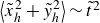 $\left \langle \tilde {x}_{{h}}^2 + \tilde {y}_{{h}}^2 \right \rangle \sim \tilde {t}^2$
appears. The crossover time reflects a dynamical transition, where rotation is governed by gravitational torque when it is large, and by rotational diffusion when the torque is small. The ballistic behaviour in MSD remains valid even when gravitational torque is present, indicating that the torque does not sufficiently alter sustained ballistic motion.
$\left \langle \tilde {x}_{{h}}^2 + \tilde {y}_{{h}}^2 \right \rangle \sim \tilde {t}^2$
appears. The crossover time reflects a dynamical transition, where rotation is governed by gravitational torque when it is large, and by rotational diffusion when the torque is small. The ballistic behaviour in MSD remains valid even when gravitational torque is present, indicating that the torque does not sufficiently alter sustained ballistic motion.
The most important feature of particles with centre offset is that they exhibit a larger sedimentation velocity (figure 3
a) than spheres and a larger diffusivity (figure 5
c,d) than those with no centre offset. The maximum diffusivity occurs around the same torque value of $\alpha \sim 2$
for both prolate and oblate spheroids, as well as for both horizontal and vertical diffusivities. The value
$\alpha \sim 2$
for both prolate and oblate spheroids, as well as for both horizontal and vertical diffusivities. The value $\alpha \sim 2$
could be frequently accessible in practice by changing the mass distribution inside the particles. Plankton, erythrocytes, micrometre-scale sediments, etc., could use this feature to accelerate their mobility (translational velocity or diffusivity) by tuning the centre offset.
$\alpha \sim 2$
could be frequently accessible in practice by changing the mass distribution inside the particles. Plankton, erythrocytes, micrometre-scale sediments, etc., could use this feature to accelerate their mobility (translational velocity or diffusivity) by tuning the centre offset.
Acknowledgements
The authors are grateful for the support of the National Natural Science Foundation of China (NSFC), Wenzhou Institute, University of Chinese Academy of Sciences and Oujiang Laboratory.
Funding
National Natural Science Foundation of China (NSFC; nos. 22403021, 12247174, 12174390 and 12150610463) and Wenzhou Institute, University of Chinese Academy of Sciences (nos. WIUCASQD2022004 and WIUCASQD2020002) and Oujiang Laboratory (no. OJQDSP2022018).
Declaration of interests
The authors report no conflict of interest.
Appendix A. Onsager’s variational principle
The probability distribution $\psi (\boldsymbol{R}_{{h}}, \boldsymbol{n}, t)$
satisfies the conservation equation (Doi & Edwards Reference Doi and Edwards1986),
$\psi (\boldsymbol{R}_{{h}}, \boldsymbol{n}, t)$
satisfies the conservation equation (Doi & Edwards Reference Doi and Edwards1986),
 \begin{equation} \frac {\partial \psi }{\partial t} = -\frac {\partial }{\partial \boldsymbol{R}_{{h}}}\boldsymbol{\cdot }\left (\boldsymbol{u}\psi \right ) -\mathcal{D}_{\boldsymbol{n}}\boldsymbol{\cdot }\left (\boldsymbol{\omega }\psi \right )\!, \end{equation}
and the normalisation condition $\int {\rm d}\varOmega \psi =1$
, where operator
$\int {\rm d}\varOmega \psi =1$
, where operator $\mathcal{D}_{\boldsymbol{n}}=\boldsymbol{n}\times \partial /\partial \boldsymbol{n}$
and
$\mathcal{D}_{\boldsymbol{n}}=\boldsymbol{n}\times \partial /\partial \boldsymbol{n}$
and ${\rm d}\varOmega ={\rm d}\boldsymbol{R}_{{h}} {\rm d}\boldsymbol{n}$
is the volume element in the configuration space
${\rm d}\varOmega ={\rm d}\boldsymbol{R}_{{h}} {\rm d}\boldsymbol{n}$
is the volume element in the configuration space $\varOmega$
.
$\varOmega$
.
The dissipation function of the system is the work done per unit time by the dissipative force (2.1). Since translation–rotation decoupling occurs at the hydrodynamic centre, the dissipation function can be expressed using the configuration distribution function $\psi$
as follows:
$\psi$
as follows:
 \begin{equation} \varPhi =\frac {1}{2}\int {\rm d}\varOmega \psi \left (\boldsymbol{u}\boldsymbol{\cdot }\boldsymbol{\zeta }_{{t}}\boldsymbol{\cdot }\boldsymbol{u}+\boldsymbol{\omega }\boldsymbol{\cdot }\boldsymbol{\zeta }_{{r}}\boldsymbol{\cdot }\boldsymbol{\omega }\right )\!. \end{equation}
The free energy of the system is $A = \int {\rm d}\varOmega \psi (U+k_{{B}}\kern-1pt T\ln \psi )$
, where
$A = \int {\rm d}\varOmega \psi (U+k_{{B}}\kern-1pt T\ln \psi )$
, where $U$
is given by (2.5) and (2.7) in terms of
$U$
is given by (2.5) and (2.7) in terms of $\boldsymbol{R}_{{h}}$
and
$\boldsymbol{R}_{{h}}$
and $\boldsymbol{n}$
. Combining the conservation equation (A1) with integration by parts over the configuration space yields the free-energy change rate (i.e. the time derivative of the free-energy):
$\boldsymbol{n}$
. Combining the conservation equation (A1) with integration by parts over the configuration space yields the free-energy change rate (i.e. the time derivative of the free-energy):
 \begin{align} \dot {A} &= \int {\rm d}\varOmega \dot {\psi }\left [-(M-M_{{b}})\boldsymbol{g}\boldsymbol{\cdot }\boldsymbol{R}_{{h}} -(M-M_{{b}})l_{{c}}\boldsymbol{g}\boldsymbol{\cdot }\boldsymbol{n}+k_{{B}}\kern-1pt T\ln \psi +k_{{B}}\kern-1pt T\right ] \notag \\ &=\int {\rm d}\varOmega \psi \left [\boldsymbol{u}\boldsymbol{\cdot }\left \{-(M-M_{{b}})\boldsymbol{g}+k_{{B}}\kern-1pt T\frac {\partial \ln \psi }{\partial \boldsymbol{R}_{{h}} }\right \}\right.\notag \\ &\quad\left. + \boldsymbol{\omega }\boldsymbol{\cdot }\big \{-(M-M_{{b}})l_{{c}} \boldsymbol{n}\times \boldsymbol{g}+k_{{B}}\kern-1pt T\mathcal{D}_{\boldsymbol{n}}\ln \psi \vphantom{\left \{-(M-M_{{b}})\boldsymbol{g}+k_{{B}}\kern-1pt T\frac {\partial \ln \psi }{\partial \boldsymbol{R}_{{h}} }\right \}}\big \} \right ]\!. \end{align}
Therefore, the velocities $\boldsymbol{u}$
and
$\boldsymbol{u}$
and $\boldsymbol{\omega }$
are obtained by minimising the Rayleighian of the system
$\boldsymbol{\omega }$
are obtained by minimising the Rayleighian of the system $\mathcal{R}=\varPhi +\dot {A}$
, i.e.
$\mathcal{R}=\varPhi +\dot {A}$
, i.e.
 \begin{align} \frac {\delta \mathcal{R}}{\delta \boldsymbol{u}} &= \left \{\boldsymbol{\zeta }_{{t}}\boldsymbol{\cdot }\boldsymbol{u} - (M-M_{{b}})\boldsymbol{g}+k_{{B}}\kern-1pt T\frac {\partial \ln \psi }{\partial \boldsymbol{R}_{{h}} }\right \}\psi = 0, \end{align}
 \begin{align} \frac {\delta \mathcal{R}}{\delta \boldsymbol{\omega }} &= \big \{ \boldsymbol{\zeta }_{{r}}\boldsymbol{\cdot }\boldsymbol{\omega } - (M-M_{{b}})l_{{c}} \boldsymbol{n}\times \boldsymbol{g}+k_{{B}}\kern-1pt T\mathcal{D}_{\boldsymbol{n}}\ln \psi \big \} \psi = 0. \end{align}
The equations can be solved using the Sherman–Morrison formula (Sherman & Morrison Reference Sherman and Morrison1950) to obtain
 \begin{align} \boldsymbol{u} &= -\frac {1}{\zeta _{{t}}^\perp }\left (\boldsymbol{\delta }+\frac {\zeta _{{t}}^\perp -\zeta _{{t}}^\parallel }{\zeta _{{t}}^\parallel }\boldsymbol{n}\boldsymbol{n}\right ) \boldsymbol{\cdot }\left \{ -(M-M_{{b}})\boldsymbol{g}+k_{{B}}\kern-1pt T\frac {\partial \ln \psi }{\partial \boldsymbol{R}_{{h}} }\right \}\!, \end{align}
 \begin{align} \boldsymbol{\omega } &= -\frac {1}{\zeta _{{r}}^\perp } \big \{-(M-M_{{b}})l_{{c}} \boldsymbol{n}\times \boldsymbol{g}+k_{{B}}\kern-1pt T\mathcal{D}_{\boldsymbol{n}}\ln \psi \big \}, \end{align}
where the contribution from the rotational component $\zeta _{{r}}^\parallel$
vanishes automatically due to the vector identity
$\zeta _{{r}}^\parallel$
vanishes automatically due to the vector identity $\boldsymbol{n} \times \boldsymbol{n} = \boldsymbol{0}$
. Therefore, combining (A1) and (A5) yields the Smoluchowski equation (2.9).
$\boldsymbol{n} \times \boldsymbol{n} = \boldsymbol{0}$
. Therefore, combining (A1) and (A5) yields the Smoluchowski equation (2.9).
Appendix B. The moments of $\boldsymbol{n}$

Because solving for the moment $\langle \boldsymbol{n}\boldsymbol{n}\rangle$
in (3.19) involves the moments
$\langle \boldsymbol{n}\boldsymbol{n}\rangle$
in (3.19) involves the moments $\langle \boldsymbol{n}\rangle$
and
$\langle \boldsymbol{n}\rangle$
and $\langle \boldsymbol{n}\boldsymbol{n}\boldsymbol{n}\rangle$
, the same procedure used in (2.18a
) can be applied to derive evolution equations for correlations
$\langle \boldsymbol{n}\boldsymbol{n}\boldsymbol{n}\rangle$
, the same procedure used in (2.18a
) can be applied to derive evolution equations for correlations $\langle \boldsymbol{n}\rangle$
,
$\langle \boldsymbol{n}\rangle$
, $\langle \boldsymbol{n}\boldsymbol{n}\boldsymbol{n}\rangle$
and
$\langle \boldsymbol{n}\boldsymbol{n}\boldsymbol{n}\rangle$
and $\langle \boldsymbol{n}\boldsymbol{n}\boldsymbol{n}\boldsymbol{n}\rangle$
. We have
$\langle \boldsymbol{n}\boldsymbol{n}\boldsymbol{n}\boldsymbol{n}\rangle$
. We have
 \begin{align} \frac {\partial \langle n_i\rangle }{\partial \tilde {t}} &= \langle \tilde {\mathcal{L}}^\dagger n_i\rangle = -2\langle n_i\rangle +\alpha \left (\hat {g}_i-\hat {g}_j\langle n_jn_i\rangle \right )\!, \end{align}
 \begin{align} \frac {\partial \langle n_in_jn_k\rangle }{\partial \tilde {t}} &= \langle \tilde {\mathcal{L}}^\dagger n_in_jn_k\rangle \notag \\ &= -2\left (6\langle n_in_jn_k\rangle -\delta _{\textit{ij}}\langle n_k\rangle -\delta _{\textit{ik}}\langle n_j\rangle -\delta _{\textit{jk}}\langle n_i\rangle \right ) \notag \\ &\quad +\alpha \left (\hat {g}_i\langle n_jn_k\rangle +\hat {g}_j\langle n_in_k\rangle +\hat {g}_k\langle n_in_j\rangle -3\hat {g}_l\langle n_ln_in_jn_k\rangle \right )\!, \end{align}
 \begin{align} \frac {\partial \langle n_in_jn_kn_l\rangle }{\partial \tilde {t}} &= \langle \tilde {\mathcal{L}}^\dagger n_in_jn_kn_l\rangle \notag \\ &= -2\left (10\langle n_in_jn_kn_l\rangle -\delta _{\textit{ij}}\langle n_kn_l\rangle -\delta _{\textit{ik}}\langle n_jn_l\rangle -\delta _{\textit{il}}\langle n_jn_k\rangle -\delta _{\textit{jk}}\langle n_in_l\rangle \right .\notag \\ &\quad - \left . \delta _{\textit{jl}}\langle n_in_k\rangle -\delta _{kl}\langle n_in_j\rangle \right ) +\alpha \left (\hat {g}_i\langle n_jn_kn_l\rangle +\hat {g}_j\langle n_in_kn_l\rangle \right . \notag \\ &\quad + \left . \hat {g}_k\langle n_in_jn_l\rangle +\hat {g}_l\langle n_in_jn_k\rangle -4\hat {g}_m\langle n_mn_in_jn_kn_l\rangle \right )\!, \end{align}
where $i,j,k,l,m \in \{x,y,z \}$
.
$i,j,k,l,m \in \{x,y,z \}$
.
We solve (B1) and (3.19) subject to initial conditions using the Laplace transform $\mathcal{T}[f(\tilde {t})]=\int _0^\infty {\rm d}\tilde {t} {\rm e}^{-\varsigma \tilde {t}}f(\tilde {t})$
. The transformed equations are
$\mathcal{T}[f(\tilde {t})]=\int _0^\infty {\rm d}\tilde {t} {\rm e}^{-\varsigma \tilde {t}}f(\tilde {t})$
. The transformed equations are
 \begin{align} \varsigma T_i &= -2T_i+\alpha \left (\frac {1}{\varsigma }\hat {g}_i-T_{\textit{ij}}\hat {g}_j\right )\!, \end{align}
 \begin{align} \varsigma T_{\textit{ij}} &= \frac {1}{3}\delta _{\textit{ij}}-2\left (3T_{\textit{ij}}-\frac {1}{\varsigma }\delta _{\textit{ij}}\right )+\alpha \left (T_i\hat {g}_j+T_j\hat {g}_i-2T_{\textit{ijk}}\hat {g}_k\right )\!, \end{align}
 \begin{align} \varsigma T_{\textit{ijk}} &= -2\left (6T_{\textit{ijk}}-\delta _{\textit{ij}}T_k-\delta _{\textit{ik}}T_j-\delta _{\textit{jk}}T_i\right ) \notag \\ &\quad +\alpha \left (T_{\textit{ij}}\hat {g}_k+T_{\textit{ik}}\hat {g}_j+T_{\textit{jk}}\hat {g}_i-3T_{\textit{ijkl}}\hat {g}_l\right )\!, \end{align}
 \begin{align} \varsigma T_{\textit{ijkl}} &= \frac {1}{15}\left (\delta _{\textit{ij}}\delta _{kl}+\delta _{\textit{il}}\delta _{\textit{jk}}+\delta _{\textit{ik}}\delta _{\textit{jl}}\right )-2\left (10T_{\textit{ijkl}}-\delta _{\textit{ij}}T_{kl}-\delta _{\textit{ik}}T_{\textit{jl}}-\delta _{\textit{il}}T_{\textit{jk}}-\delta _{\textit{jk}}T_{\textit{il}}\right .\notag \\ &\quad - \left . \delta _{\textit{jl}}T_{\textit{ik}}-\delta _{kl}T_{\textit{ij}}\right )+\alpha \left (T_{\textit{ijk}}\hat {g}_l+T_{\textit{ijl}}\hat {g}_k+T_{\textit{ikl}}\hat {g}_j+T_{\textit{jkl}}\hat {g}_i-4\hat {g}_mT_{\textit{ijklm}}\right )\!, \end{align}
where $T_i = \mathcal{T}[\langle n_i\rangle ]$
(at least order of
$T_i = \mathcal{T}[\langle n_i\rangle ]$
(at least order of $\alpha ^1$
),
$\alpha ^1$
), $T_{\textit{ij}} = \mathcal{T}[\langle n_in_j\rangle ]$
(at least order of
$T_{\textit{ij}} = \mathcal{T}[\langle n_in_j\rangle ]$
(at least order of $\alpha ^0$
),
$\alpha ^0$
), $T_{\textit{ijk}} = \mathcal{T}[\langle n_in_jn_k\rangle ]$
(at least order of
$T_{\textit{ijk}} = \mathcal{T}[\langle n_in_jn_k\rangle ]$
(at least order of $\alpha ^1$
) and
$\alpha ^1$
) and $T_{\textit{ijkl}} = \mathcal{T}[\langle n_in_jn_kn_l\rangle ]$
(at least order of
$T_{\textit{ijkl}} = \mathcal{T}[\langle n_in_jn_kn_l\rangle ]$
(at least order of $\alpha ^0$
). However, solving for any given moment invariably involves higher-order moments. Here, we retain only terms up to
$\alpha ^0$
). However, solving for any given moment invariably involves higher-order moments. Here, we retain only terms up to $\alpha ^2$
in (B2b). This implies we retain
$\alpha ^2$
in (B2b). This implies we retain $T_i$
and
$T_i$
and $T_{\textit{ijk}}$
to first order in
$T_{\textit{ijk}}$
to first order in $\alpha$
, while keeping
$\alpha$
, while keeping $T_{\textit{ij}}$
and
$T_{\textit{ij}}$
and $T_{\textit{ijkl}}$
to zeroth order in
$T_{\textit{ijkl}}$
to zeroth order in $\alpha$
. The zeroth-order expressions for
$\alpha$
. The zeroth-order expressions for $T_{\textit{ij}}$
and
$T_{\textit{ij}}$
and $T_{\textit{ijkl}}$
are given by
$T_{\textit{ijkl}}$
are given by
 \begin{align} T_{\textit{ij}} &= \frac {1}{3\varsigma }\delta _{\textit{ij}} +o\big(\alpha ^0\big), \end{align}
 \begin{align} T_{\textit{ijkl}} &= \frac {1}{15\varsigma }\left (\delta _{\textit{ij}}\delta _{kl}+\delta _{\textit{ik}}\delta _{\textit{jl}}+\delta _{\textit{il}}\delta _{\textit{jk}}\right ) +o\big(\alpha ^0\big). \end{align}
The first-order expressions for $T_i$
and
$T_i$
and $T_{\textit{ijk}}$
, derived by inserting (B3) into (B2a
) and (B2c
), are given as follows:
$T_{\textit{ijk}}$
, derived by inserting (B3) into (B2a
) and (B2c
), are given as follows:
 \begin{align} T_i &= \frac {2\alpha }{3\varsigma (\varsigma +2)}\hat {g}_i +o\big(\alpha ^1\big), \end{align}
 \begin{align} T_{\textit{ijk}} &= \frac {2\alpha }{15\varsigma (\varsigma +2)}\left (\delta _{\textit{ij}}\hat {g}_k+\delta _{\textit{ik}}\hat {g}_j+\delta _{\textit{jk}}\hat {g}_i\right ) +o\big(\alpha ^1\big). \end{align}
Therefore, the second-order expression for $T_{\textit{ij}}$
, derived by inserting (B4) into (B2b
), is given by
$T_{\textit{ij}}$
, derived by inserting (B4) into (B2b
), is given by
 \begin{equation} T_{\textit{ij}} = \frac {1}{3\varsigma }\delta _{\textit{ij}}+\frac {4\alpha ^2}{5\varsigma (\varsigma +2)(\varsigma +6)}\left (\hat {g}_i\hat {g}_j-\frac {1}{3}\delta _{\textit{ij}}\right )+o\big(\alpha ^2\big). \end{equation}
The inverse Laplace transform gives the solution (3.20).
Appendix C. The moments of
$\boldsymbol{n}$
and
$\tilde {\boldsymbol{R}}_{{h}}$


Applying (2.18a ) to (3.1b ) and to the square of (3.1a ) yields
 \begin{align} \frac {\partial \left \langle \tilde {x}_{{h}}^2+\tilde {y}_{{h}}^2 \right \rangle }{\partial \tilde {t}} &= \left \langle \tilde {\mathcal{L}}^\dagger \left \{(\boldsymbol{\delta }-\hat {\boldsymbol{g}}\hat {\boldsymbol{g}})\boldsymbol{\cdot }[\tilde {\boldsymbol{R}}_{{h}}\big(\tilde {t}\big)-\tilde {\boldsymbol{R}}_{{h}}(0)] \right \}^2 \right \rangle \notag \\ &= 2\tilde {D}^\perp \left [2+\chi \big (1- \hat {\boldsymbol{g}}\boldsymbol{\cdot }\left \langle \boldsymbol{n}\boldsymbol{n} \right \rangle \boldsymbol{\cdot }\hat {\boldsymbol{g}} \big )\right ] +2\beta \chi \mathcal{H}^1, \end{align}
 \begin{align} \frac {\partial \langle \left [\tilde {z}_{{h}}-\langle \tilde {z}_{{h}}\rangle \right ]^2\rangle }{\partial \tilde {t}} &= \left \langle \tilde {\mathcal{L}}^\dagger \left \{\hat {\boldsymbol{g}}\boldsymbol{\cdot }[\tilde {\boldsymbol{R}}_{{h}}\big(\tilde {t}\big)-\tilde {\boldsymbol{R}}_{{h}}(0)]-\hat {\boldsymbol{g}}\boldsymbol{\cdot }\left \langle \tilde {\boldsymbol{R}}_{{h}}\big(\tilde {t}\big)-\tilde {\boldsymbol{R}}_{{h}}(0)\right \rangle \right \}^2 \right \rangle \notag \\ &= 2\tilde {D}^\perp \big ( 1+\chi \hat {\boldsymbol{g}}\boldsymbol{\cdot }\left \langle \boldsymbol{n}\boldsymbol{n} \right \rangle \boldsymbol{\cdot }\hat {\boldsymbol{g}} \big )+2\beta \chi \mathcal{V}^1, \end{align}
where $\mathcal{H}^1= \langle \hat {\boldsymbol{g}}\boldsymbol{\cdot }\boldsymbol{n}\boldsymbol{n} \boldsymbol{\cdot }(\boldsymbol{\delta }-\hat {\boldsymbol{g}}\hat {\boldsymbol{g}}) \boldsymbol{\cdot }[\tilde {\boldsymbol{R}}_{{h}}(\tilde {t})-\tilde {\boldsymbol{R}}_{{h}}(0)] \rangle$
and
$\mathcal{H}^1= \langle \hat {\boldsymbol{g}}\boldsymbol{\cdot }\boldsymbol{n}\boldsymbol{n} \boldsymbol{\cdot }(\boldsymbol{\delta }-\hat {\boldsymbol{g}}\hat {\boldsymbol{g}}) \boldsymbol{\cdot }[\tilde {\boldsymbol{R}}_{{h}}(\tilde {t})-\tilde {\boldsymbol{R}}_{{h}}(0)] \rangle$
and $\mathcal{V}^1= \langle \hat {\boldsymbol{g}}\boldsymbol{\cdot }\boldsymbol{n}\boldsymbol{n} \boldsymbol{\cdot }\hat {\boldsymbol{g}}\hat {\boldsymbol{g}} \boldsymbol{\cdot }[\tilde {\boldsymbol{R}}_{{h}}(\tilde {t})- \tilde {\boldsymbol{R}}_{{h}}(0)] \rangle -\hat {\boldsymbol{g}}\boldsymbol{\cdot }\langle \boldsymbol{n}\boldsymbol{n}\rangle \boldsymbol{\cdot }\hat {\boldsymbol{g}}\hat {\boldsymbol{g}} \boldsymbol{\cdot } \langle \tilde {\boldsymbol{R}}_{{h}}(\tilde {t})-\tilde {\boldsymbol{R}}_{{h}}(0) \rangle$
.
$\mathcal{V}^1= \langle \hat {\boldsymbol{g}}\boldsymbol{\cdot }\boldsymbol{n}\boldsymbol{n} \boldsymbol{\cdot }\hat {\boldsymbol{g}}\hat {\boldsymbol{g}} \boldsymbol{\cdot }[\tilde {\boldsymbol{R}}_{{h}}(\tilde {t})- \tilde {\boldsymbol{R}}_{{h}}(0)] \rangle -\hat {\boldsymbol{g}}\boldsymbol{\cdot }\langle \boldsymbol{n}\boldsymbol{n}\rangle \boldsymbol{\cdot }\hat {\boldsymbol{g}}\hat {\boldsymbol{g}} \boldsymbol{\cdot } \langle \tilde {\boldsymbol{R}}_{{h}}(\tilde {t})-\tilde {\boldsymbol{R}}_{{h}}(0) \rangle$
.
Here, we focus on calculating the correlation $\mathcal{H}^1$
(and
$\mathcal{H}^1$
(and $\mathcal{V}^1$
) using two equivalent approaches. One approach is an integral method that uses the Green’s function to provide an approximate solution valid across the entire range of
$\mathcal{V}^1$
) using two equivalent approaches. One approach is an integral method that uses the Green’s function to provide an approximate solution valid across the entire range of $\alpha$
. The other approach is a differential method that employs an iterative procedure to yield exact solutions up to a finite order in
$\alpha$
. The other approach is a differential method that employs an iterative procedure to yield exact solutions up to a finite order in $\alpha$
.
$\alpha$
.
(1) Eigenfunction expansion method: differentiating $\mathcal{H}^1$
(and
$\mathcal{H}^1$
(and $\mathcal{V}^1$
) with respect to the past time
$\mathcal{V}^1$
) with respect to the past time $\tilde {t}^\prime$
yields
$\tilde {t}^\prime$
yields
 \begin{align} \frac {\partial \big \langle \hat {\boldsymbol{g}}\boldsymbol{\cdot }\boldsymbol{n}\boldsymbol{n}\boldsymbol{\cdot }(\boldsymbol{\delta }-\hat {\boldsymbol{g}}\hat {\boldsymbol{g}})\boldsymbol{\cdot }(\tilde {\boldsymbol{R}}_{{h}}-\tilde {\boldsymbol{R}}_{{h}}^\prime)\big \rangle }{\partial \tilde {t}^\prime}&=\left \langle \tilde {\mathcal{L}}^{\dagger \prime }\hat {\boldsymbol{g}}\boldsymbol{\cdot }\boldsymbol{n}\boldsymbol{n}\boldsymbol{\cdot }(\boldsymbol{\delta }-\hat {\boldsymbol{g}}\hat {\boldsymbol{g}})\boldsymbol{\cdot }(\tilde {\boldsymbol{R}}_{{h}}-\tilde {\boldsymbol{R}}_{{h}}^\prime)\right \rangle \notag \\ &=-\beta \chi \left \langle \hat {\boldsymbol{g}}\boldsymbol{\cdot }\boldsymbol{n}\boldsymbol{n}\boldsymbol{\cdot }(\boldsymbol{\delta }-\hat {\boldsymbol{g}}\hat {\boldsymbol{g}})\boldsymbol{\cdot }\boldsymbol{n}^\prime\boldsymbol{n}^\prime\boldsymbol{\cdot }\hat {\boldsymbol{g}}\right \rangle , \end{align}
 \begin{align} \frac {\partial \big \langle \hat {\boldsymbol{g}}\boldsymbol{\cdot }\boldsymbol{n}\boldsymbol{n}\boldsymbol{\cdot }\hat {\boldsymbol{g}}\hat {\boldsymbol{g}}\boldsymbol{\cdot }(\tilde {\boldsymbol{R}}_{{h}}-\tilde {\boldsymbol{R}}_{{h}}^\prime)\big \rangle }{\partial \tilde {t}^\prime}&=\left \langle \tilde {\mathcal{L}}^{\dagger \prime }\hat {\boldsymbol{g}}\boldsymbol{\cdot }\boldsymbol{n}\boldsymbol{n}\boldsymbol{\cdot }\hat {\boldsymbol{g}}\hat {\boldsymbol{g}}\boldsymbol{\cdot }(\tilde {\boldsymbol{R}}_{{h}}-\tilde {\boldsymbol{R}}_{{h}}^\prime)\right \rangle \notag \\ &=-\beta \hat {\boldsymbol{g}}\boldsymbol{\cdot }\left \langle \boldsymbol{n}\boldsymbol{n}\right \rangle \boldsymbol{\cdot }\hat {\boldsymbol{g}} -\beta \chi \left \langle \hat {\boldsymbol{g}}\boldsymbol{\cdot }\boldsymbol{n}\boldsymbol{n}\boldsymbol{\cdot }\hat {\boldsymbol{g}}\hat {\boldsymbol{g}}\boldsymbol{\cdot }\boldsymbol{n}^\prime\boldsymbol{n}^\prime\boldsymbol{\cdot }\hat {\boldsymbol{g}}\right \rangle , \end{align}
where $\tilde {\mathcal{L}}^{\dagger \prime }$
denotes the operator
$\tilde {\mathcal{L}}^{\dagger \prime }$
denotes the operator $\tilde {\mathcal{L}}^\dagger$
acting on functions defined over the configuration
$\tilde {\mathcal{L}}^\dagger$
acting on functions defined over the configuration $\tilde {\varOmega }^\prime$
. Integrating both sides of (C2a
) and (C2b
) yields the solutions
$\tilde {\varOmega }^\prime$
. Integrating both sides of (C2a
) and (C2b
) yields the solutions $\mathcal{H}^1 = 2\beta \chi \varXi (\tilde {t};\alpha )$
and
$\mathcal{H}^1 = 2\beta \chi \varXi (\tilde {t};\alpha )$
and $\mathcal{V}^1 = \beta \chi \varTheta (\tilde {t};\alpha )$
, respectively, with
$\mathcal{V}^1 = \beta \chi \varTheta (\tilde {t};\alpha )$
, respectively, with
 \begin{align} \varXi (\tilde {t};\alpha ) &= \frac {1}{2} \int _0^{\tilde {t}}{\rm d}\tilde {t}^\prime\left \langle \hat {\boldsymbol{g}}\boldsymbol{\cdot }\boldsymbol{n}\boldsymbol{n}\boldsymbol{\cdot }(\boldsymbol{\delta }-\hat {\boldsymbol{g}}\hat {\boldsymbol{g}})\boldsymbol{\cdot }\boldsymbol{n}^\prime\boldsymbol{n}^\prime \boldsymbol{\cdot }\hat {\boldsymbol{g}}\right \rangle\! , \end{align}
 \begin{align} \varTheta (\tilde {t};\alpha ) &= \int _0^{\tilde {t}}{\rm d}\tilde {t}^\prime\left [\left \langle \hat {\boldsymbol{g}}\boldsymbol{\cdot }\boldsymbol{n}\boldsymbol{n}\boldsymbol{\cdot }\hat {\boldsymbol{g}}\hat {\boldsymbol{g}}\boldsymbol{\cdot }\boldsymbol{n}^\prime\boldsymbol{n}^\prime \boldsymbol{\cdot }\hat {\boldsymbol{g}}\right \rangle -\hat {\boldsymbol{g}}\boldsymbol{\cdot }\left \langle \boldsymbol{n}\boldsymbol{n}\right \rangle \boldsymbol{\cdot }\hat {\boldsymbol{g}}\hat {\boldsymbol{g}}\boldsymbol{\cdot }\left \langle \boldsymbol{n}^\prime\boldsymbol{n}^\prime \right \rangle \boldsymbol{\cdot }\hat {\boldsymbol{g}}\right ]\!, \end{align}
where the solution of (3.2) has been used in (C3b ). This solution demonstrates that the particle displacement correlation can be obtained by time-integrating the translational velocity within the Langevin framework, where the velocity’s drift term scales proportionally with the translational resistance coefficients. Since translational resistance coefficients depend on particle orientation, the net displacement accumulates over the particle’s entire orientation history. Combining the solution in (C3a ) with (C1a ) yields (3.4). Similarly, combining the solution in (C3b ) with (C1b ) yields (3.3).
In particular, the orientation-history integral $\varXi (\tilde {t};\alpha )$
(or
$\varXi (\tilde {t};\alpha )$
(or $\varTheta (\tilde {t};\alpha )$
) converges to a constant
$\varTheta (\tilde {t};\alpha )$
) converges to a constant $\varXi _{\textit{ss}}(\alpha )$
(or
$\varXi _{\textit{ss}}(\alpha )$
(or $\varTheta _{\textit{ss}}(\alpha )$
) at long times for fixed
$\varTheta _{\textit{ss}}(\alpha )$
) at long times for fixed $\alpha$
, where
$\alpha$
, where $\varXi _{\textit{ss}}(\alpha )$
and
$\varXi _{\textit{ss}}(\alpha )$
and $\varTheta _{\textit{ss}}(\alpha )$
are defined by (3.24a
) and (3.24b
). Using the Green’s function from (3.9) and incorporating the spherical coordinate relationships
$\varTheta _{\textit{ss}}(\alpha )$
are defined by (3.24a
) and (3.24b
). Using the Green’s function from (3.9) and incorporating the spherical coordinate relationships $n_x=\sin \theta \cos \phi$
and
$n_x=\sin \theta \cos \phi$
and $n_z=\cos \theta$
, we derive
$n_z=\cos \theta$
, we derive
 \begin{align} \varXi _{\textit{ss}}(\alpha ) &=\sum _{p=1}^\infty \left (\int _0^{2\pi } {\rm d}\phi \int _0^\pi {\rm d}\theta \sin \theta \psi _p(\theta ,\phi )\sin \theta \cos \phi \cos \theta \right )^2 \frac {1}{\lambda _p} , \end{align}
 \begin{align} \varTheta _{\textit{ss}}(\alpha ) &=\sum _{p=1}^\infty \left (\int _0^{2\pi } {\rm d}\phi \int _0^\pi {\rm d}\theta \sin \theta \psi _p(\theta ,\phi )\cos ^2\theta \right )^2 \frac {1}{\lambda _p} . \end{align}
Note that the $p=0$
term vanishes because
$p=0$
term vanishes because $\psi _0$
is independent of
$\psi _0$
is independent of $\phi$
in (C4a
) and cancellation appears in (C4b
). For
$\phi$
in (C4a
) and cancellation appears in (C4b
). For $p \ne 0$
(
$p \ne 0$
( $p=1,2,\dots ,g$
), we assumed that each eigenfunction
$p=1,2,\dots ,g$
), we assumed that each eigenfunction $\psi _p(\theta ,\phi )$
is approximated by a linear combination of spherical harmonics
$\psi _p(\theta ,\phi )$
is approximated by a linear combination of spherical harmonics $Y_l^m(\theta ,\phi )$
with weight function
$Y_l^m(\theta ,\phi )$
with weight function $\psi _{\textit{ss}}^{1/2}(\theta )$
, truncated to
$\psi _{\textit{ss}}^{1/2}(\theta )$
, truncated to $g$
terms, i.e.
$g$
terms, i.e.
 \begin{equation} \psi _p(\theta ,\phi ) = \psi _{\textit{ss}}^{1/2}(\theta ) \sum _{l=0}^g\sum _{m=-l}^l a_{l,m}^pY_l^m(\theta ,\phi ), \end{equation}
with
 \begin{equation} Y_l^m(\theta ,\phi )=\sqrt {\frac {(2 l+1) (l-m)!}{4 \pi (l+m)!}} P_l^m(\cos \theta ) {\rm e}^{\mathrm{i} m\phi }, \end{equation}
where $P_l^m(\cos \theta )$
are the associated Legendre functions. A technical consideration is that the operator
$P_l^m(\cos \theta )$
are the associated Legendre functions. A technical consideration is that the operator $\tilde {\mathcal{L}}_{{sp}}$
in the eigenequation (3.10) is non-Hermitian. To achieve a stable numerical algorithm, the operator can be transformed into a Hermitian operator by introducing the weight function
$\tilde {\mathcal{L}}_{{sp}}$
in the eigenequation (3.10) is non-Hermitian. To achieve a stable numerical algorithm, the operator can be transformed into a Hermitian operator by introducing the weight function $\psi _{\textit{ss}}^{1/2}(\theta )$
in (C5a
) (Risken Reference Risken1989). Additionally, because
$\psi _{\textit{ss}}^{1/2}(\theta )$
in (C5a
) (Risken Reference Risken1989). Additionally, because $n_x$
depends on
$n_x$
depends on $\cos \phi$
in (C4a
), only the
$\cos \phi$
in (C4a
), only the $m=1$
term survives in the summation over
$m=1$
term survives in the summation over $m$
due to the orthogonality of trigonometric functions. However, because
$m$
due to the orthogonality of trigonometric functions. However, because $n_z$
is independent of
$n_z$
is independent of $\phi$
in (C4b
), only the
$\phi$
in (C4b
), only the $m=0$
term survives in the summation over
$m=0$
term survives in the summation over $m$
for the vertical dispersion. Therefore, by inserting the eigenfunction form from (C5a
), with
$m$
for the vertical dispersion. Therefore, by inserting the eigenfunction form from (C5a
), with $m=1$
for horizontal dispersion and
$m=1$
for horizontal dispersion and $m=0$
for vertical dispersion, into the eigenequation (3.10), we obtain the first
$m=0$
for vertical dispersion, into the eigenequation (3.10), we obtain the first $g$
approximate solutions
$g$
approximate solutions $\lambda _p^m$
and coefficients
$\lambda _p^m$
and coefficients $a_{i,m}^p$
from
$a_{i,m}^p$
from
 \begin{align} \sum _{j=1}^g \mathcal{M}_{\textit{ij}}^ma_{j,m}^p =\lambda _p^m a_{i,m}^p, \qquad (m=0,1). \end{align}
The eigenvectors $a_{i,m}^p$
are orthonormalised, i.e.
$a_{i,m}^p$
are orthonormalised, i.e. $\sum _{i=1}^ga_{i,m}^pa_{i,m}^q=\delta _{p,q}$
. Here
$\sum _{i=1}^ga_{i,m}^pa_{i,m}^q=\delta _{p,q}$
. Here $\mathcal{M}_{\textit{ij}}^m$
is the symmetric part (
$\mathcal{M}_{\textit{ij}}^m$
is the symmetric part ( $(\boldsymbol{M}+\boldsymbol{M}^T)/2$
) of the following
$(\boldsymbol{M}+\boldsymbol{M}^T)/2$
) of the following $g \times g$
matrix:
$g \times g$
matrix:
 \begin{align} M_{kl}^0&= \left [k(k+1)+\frac {(k^2+k-1)\alpha ^2}{2(2k-1)(2k+3)}\right ] \delta _{k,l}+2\alpha \sqrt {\frac {(k+1)^2}{(2k+1)(2k+3)}}\delta _{k,l-1} \notag \\ &\quad -\frac {\alpha ^2}{2}\sqrt {\frac {(k+1)^2 (k+2)^2}{(2 k+1) (2 k+3)^2 (2 k+5)}}\delta _{k,l-2}, \qquad (k,l = 0,1,2,\ldots ,g-1), \end{align}
 \begin{align} M_{kl}^1&= \left [k(k+1)+\frac {(k^2+k)\alpha ^2}{2(2k-1)(2k+3)}\right ] \delta _{k,l}+2\alpha \sqrt {\frac {k(k+2)}{(2k+1)(2k+3)}}\delta _{k,l-1}\notag \\ &\quad -\frac {\alpha ^2}{2}\sqrt {\frac {k (k+1) (k+2) (k+3)}{(2 k+1) (2 k+3)^2 (2 k+5)}}\delta _{k,l-2}, \qquad (k,l = 1,2,3,\ldots ,g), \end{align}
where $\delta _{k,l}$
is the Kronecker delta. In this work,
$\delta _{k,l}$
is the Kronecker delta. In this work, $g=35$
is sufficient to obtain numerically converged solutions.
$g=35$
is sufficient to obtain numerically converged solutions.
(2) Iterative method: the equivalent differential equation for $\mathcal{H}^1$
can be derived by directly applying (2.18a
) to the correlation function
$\mathcal{H}^1$
can be derived by directly applying (2.18a
) to the correlation function $\mathcal{H}^m=\langle (\hat {\boldsymbol{g}}\boldsymbol{\cdot }\boldsymbol{n})^m\boldsymbol{n}\boldsymbol{\cdot }(\boldsymbol{\delta }-\hat {\boldsymbol{g}}\hat {\boldsymbol{g}})\boldsymbol{\cdot }[\tilde {\boldsymbol{R}}_{{h}}(\tilde {t})-\tilde {\boldsymbol{R}}_{{h}}(0)]\rangle$
:
$\mathcal{H}^m=\langle (\hat {\boldsymbol{g}}\boldsymbol{\cdot }\boldsymbol{n})^m\boldsymbol{n}\boldsymbol{\cdot }(\boldsymbol{\delta }-\hat {\boldsymbol{g}}\hat {\boldsymbol{g}})\boldsymbol{\cdot }[\tilde {\boldsymbol{R}}_{{h}}(\tilde {t})-\tilde {\boldsymbol{R}}_{{h}}(0)]\rangle$
:
 \begin{align} \frac {\partial \mathcal{H}^m}{\partial \tilde {t}} &= (m-1)m\mathcal{H}^{m-2}-(m+1)(m+2)\mathcal{H}^m+\alpha \left [m\mathcal{H}^{m-1}-(m+1)\mathcal{H}^{m+1}\right ]\notag \\ &\quad +\beta \chi \left (\langle (\hat {\boldsymbol{g}}\boldsymbol{\cdot }\boldsymbol{n})^{m+1}\rangle -\langle (\hat {\boldsymbol{g}}\boldsymbol{\cdot }\boldsymbol{n})^{m+3}\rangle \right )\!, \end{align}
where $m=0,1,2,\dotsc$
. Therefore, the moments
$m=0,1,2,\dotsc$
. Therefore, the moments $\langle (\hat {\boldsymbol{g}}\boldsymbol{\cdot }\boldsymbol{n})^m\rangle$
govern translational diffusion. Similarly, we define
$\langle (\hat {\boldsymbol{g}}\boldsymbol{\cdot }\boldsymbol{n})^m\rangle$
govern translational diffusion. Similarly, we define $\mathcal{F}^m=\langle (\hat {\boldsymbol{g}}\boldsymbol{\cdot }\boldsymbol{n})^m\hat {\boldsymbol{g}}\boldsymbol{\cdot }[\tilde {\boldsymbol{R}}_{{h}}(\tilde {t})-\tilde {\boldsymbol{R}}_{{h}}(0)]\rangle$
. Thus,
$\mathcal{F}^m=\langle (\hat {\boldsymbol{g}}\boldsymbol{\cdot }\boldsymbol{n})^m\hat {\boldsymbol{g}}\boldsymbol{\cdot }[\tilde {\boldsymbol{R}}_{{h}}(\tilde {t})-\tilde {\boldsymbol{R}}_{{h}}(0)]\rangle$
. Thus, $\mathcal{V}^1 = \mathcal{F}^2-\langle (\hat {\boldsymbol{g}}\boldsymbol{\cdot }\boldsymbol{n})^2\rangle \mathcal{F}^0$
. Applying (2.18a
) to
$\mathcal{V}^1 = \mathcal{F}^2-\langle (\hat {\boldsymbol{g}}\boldsymbol{\cdot }\boldsymbol{n})^2\rangle \mathcal{F}^0$
. Applying (2.18a
) to $\mathcal{F}^m$
yields
$\mathcal{F}^m$
yields
 \begin{align} \frac {\partial \mathcal{F}^m}{\partial \tilde {t}} &= m\left [(m-1)\mathcal{F}^{m-2}-(m+1)\mathcal{F}^m+\alpha (\mathcal{F}^{m-1}-\mathcal{F}^{m+1})\right ]\notag \\ &\quad +\beta \left [\langle (\hat {\boldsymbol{g}}\boldsymbol{\cdot }\boldsymbol{n})^m\rangle +\chi \langle (\hat {\boldsymbol{g}}\boldsymbol{\cdot }\boldsymbol{n})^{m+2}\rangle \right ]\!, \end{align}
where $m=0,1,2,\dotsc$
.
$m=0,1,2,\dotsc$
.
In the long-time limit, we expect $\partial \mathcal{H}^m/\partial \tilde {t}=0$
. Setting
$\partial \mathcal{H}^m/\partial \tilde {t}=0$
. Setting $m=0$
in (C8) then yields an equation for
$m=0$
in (C8) then yields an equation for $\mathcal{H}^1$
. Therefore,
$\mathcal{H}^1$
. Therefore, $\varXi _{\textit{ss}}(\alpha )$
admits the alternative expression:
$\varXi _{\textit{ss}}(\alpha )$
admits the alternative expression:
 \begin{align} \varXi _{\textit{ss}}(\alpha ) &= \frac {\langle (\hat {\boldsymbol{g}}\boldsymbol{\cdot }\boldsymbol{n})^1\rangle _{\textit{ss}}-\langle (\hat {\boldsymbol{g}}\boldsymbol{\cdot }\boldsymbol{n})^3\rangle _{\textit{ss}}}{2\alpha }-\frac {f(\alpha )}{\sinh \alpha }, \end{align}
where
 \begin{align} \langle (\hat {\boldsymbol{g}}\boldsymbol{\cdot }\boldsymbol{n})^m\rangle _{\textit{ss}} = \lim _{\tilde {t} \to \infty } \langle (\hat {\boldsymbol{g}}\boldsymbol{\cdot }\boldsymbol{n})^m\rangle &= \frac {\alpha }{2\sinh \alpha } \int _{-1}^{1} {\rm d}\xi {\rm e}^{\alpha \xi }\xi ^{m}, \end{align}
 \begin{align} f(\alpha ) = \frac {\sinh \alpha }{\beta \chi \alpha }\mathcal{H}^0_{\textit{ss}} &= \sum _{i=1,\text{odd}}^\infty p_0^i \alpha ^i , \end{align}
with coefficients determined iteratively by
 \begin{align} p_m^i &= \frac {1}{(m+1)(m+2)}\left [(m-1)mp_{m-2}^i+mp_{m-1}^{i-1}-(m+1)p_{m+1}^{i-1}+c_m^i\right ]\!, \end{align}
 \begin{align} p_m^0 &= \frac {1}{3(m+2)(m+4)}, \end{align}
 \begin{align} c_m^i &= \frac {2}{i!(i+m+2)(i+m+4)}. \end{align}
The two approaches in (C4) and (C10) yield equivalent results if $g \to \infty$
.
$g \to \infty$
.
Modelling the transient behaviour of $\mathcal{H}^m$
requires the time evolution of
$\mathcal{H}^m$
requires the time evolution of $\langle (\hat {\boldsymbol{g}}\boldsymbol{\cdot }\boldsymbol{n})^m\rangle$
in (C8). Again, solving for the current moment of order
$\langle (\hat {\boldsymbol{g}}\boldsymbol{\cdot }\boldsymbol{n})^m\rangle$
in (C8). Again, solving for the current moment of order $m$
invariably involves the higher-order moment
$m$
invariably involves the higher-order moment $m+1$
. Therefore, applying the same procedure used in (B3a
)–(B4b
), the solution for
$m+1$
. Therefore, applying the same procedure used in (B3a
)–(B4b
), the solution for $\langle (\hat {\boldsymbol{g}}\boldsymbol{\cdot }\boldsymbol{n})^m\rangle$
up to order of
$\langle (\hat {\boldsymbol{g}}\boldsymbol{\cdot }\boldsymbol{n})^m\rangle$
up to order of $\alpha ^2$
can be obtained either from (B1) via contractions with
$\alpha ^2$
can be obtained either from (B1) via contractions with $\hat {\boldsymbol{g}}$
or directly from (2.18a
). The initial conditions are set to the equilibrium values corresponding to zero gravity, i.e. the equilibrium moments are
$\hat {\boldsymbol{g}}$
or directly from (2.18a
). The initial conditions are set to the equilibrium values corresponding to zero gravity, i.e. the equilibrium moments are $\langle (\hat {\boldsymbol{g}}\boldsymbol{\cdot }\boldsymbol{n})^m\rangle _{{eq}} = 1/(m+1)$
for even
$\langle (\hat {\boldsymbol{g}}\boldsymbol{\cdot }\boldsymbol{n})^m\rangle _{{eq}} = 1/(m+1)$
for even $m$
and
$m$
and $0$
for odd
$0$
for odd $m$
, which can be determined from
$m$
, which can be determined from $\left .\langle (\hat {\boldsymbol{g}}\boldsymbol{\cdot }\boldsymbol{n})^m\rangle _{\textit{ss}}\right |_{\alpha =0}$
. Using Laplace transforms, the time evolutions of
$\left .\langle (\hat {\boldsymbol{g}}\boldsymbol{\cdot }\boldsymbol{n})^m\rangle _{\textit{ss}}\right |_{\alpha =0}$
. Using Laplace transforms, the time evolutions of $\langle (\hat {\boldsymbol{g}}\boldsymbol{\cdot }\boldsymbol{n})^m\rangle$
up to the order of
$\langle (\hat {\boldsymbol{g}}\boldsymbol{\cdot }\boldsymbol{n})^m\rangle$
up to the order of $\alpha ^2$
are given by
$\alpha ^2$
are given by
 \begin{equation} \mathcal{T}\left [\langle (\hat {\boldsymbol{g}}\boldsymbol{\cdot }\boldsymbol{n})^m\rangle \right ] = \begin{cases} C_m^0(\varsigma )+C_m^2(\varsigma )\alpha ^2, & m=0,2,4,\dotsc \\[2pt] C_m^1(\varsigma )\alpha , & m=1,3,5,\dotsc ,\end{cases} \end{equation}
where
 \begin{align} C_m^0 &= \frac {1}{(m+1)\varsigma }, \end{align}
 \begin{align} C_m^1 &= \frac {2}{(m+2)\varsigma (\varsigma +2)}, \end{align}
 \begin{align} C_m^2 &= \frac {4m}{(m+1)(m+3)\varsigma (\varsigma +2)(\varsigma +6)}. \end{align}
Therefore, the transient behaviour of $\mathcal{H}^m$
can be calculated using the solution in (C13). The solution for
$\mathcal{H}^m$
can be calculated using the solution in (C13). The solution for $\mathcal{H}^m$
up to order of
$\mathcal{H}^m$
up to order of $\alpha ^2$
is obtained by
$\alpha ^2$
is obtained by
 \begin{equation} \mathcal{T}\left [\mathcal{H}^m\right ] = \begin{cases} \beta \chi P_m^1(\varsigma )\alpha , & m=0,2,4, \dotsc \\[2pt] \beta \chi \left [P_m^0(\varsigma )+P_m^2(\varsigma )\alpha ^2\right ]\!, & m=1,3,5, \dotsc .\end{cases} \end{equation}
Applying a similar procedure to $\mathcal{F}^m$
, we obtain
$\mathcal{F}^m$
, we obtain
 \begin{equation} \mathcal{T}\left [\mathcal{F}^m\right ] = \begin{cases} \beta \left [Q_m^0(\varsigma ,\chi )+Q_m^2(\varsigma ,\chi )\alpha ^2\right ]\!, & m=0,2,4,\dots \\[2pt] \beta Q_m^1(\varsigma ,\chi )\alpha , & m=1,3,5,\dots ,\end{cases} \end{equation}
where the coefficients are determined iteratively by
 \begin{align} P_m^0 &= \frac {1}{\varsigma \!+\!(m+1)(m+2)}\left [(m-1)mP_{m-2}^0+C_{m+1}^0-C_{m+3}^0\right ]\!, \end{align}
 \begin{align} P_m^1 &= \frac {1}{\varsigma \!+\!(m+1)(m+2)}\left [(m-1)mP_{m-2}^1+C_{m+1}^1-C_{m+3}^1+mP_{m-1}^0-(m+1)P_{m+1}^0\!\right ]\!, \end{align}
 \begin{align} P_m^2 &= \frac {1}{\varsigma \!+\!(m+1)(m+2)}\left [(m-1)mP_{m-2}^2+C_{m+1}^2-C_{m+3}^2+mP_{m-1}^1-(m+1)P_{m+1}^1\!\right ]\!, \end{align}
 \begin{align} Q_m^0 &= \frac {1}{\varsigma +m(m+1)}\left [(m-1)mQ_{m-2}^0+\left (C_m^0+\chi C_{m+2}^0\right )\right ]\!, \end{align}
 \begin{align} Q_m^1 &= \frac {1}{\varsigma +m(m+1)}\left [(m-1)mQ_{m-2}^1+\left (C_m^1+\chi C_{m+2}^1\right )+m\left (Q_{m-1}^0-Q_{m+1}^0\right )\right ]\!, \end{align}
 \begin{align} Q_m^2 &= \frac {1}{\varsigma +m(m+1)}\left [(m-1)mQ_{m-2}^2+\left (C_m^2+\chi C_{m+2}^2\right )+m\left (Q_{m-1}^1-Q_{m+1}^1\right )\right ]\!. \end{align}
Here, we explicitly present selected results from (C15a ) and (C15b ):
 \begin{align} \mathcal{T}\left [\mathcal{H}^0\right ] &= 2\beta \chi \frac {\varsigma +10}{15\varsigma (\varsigma +2)^2 (\varsigma +6)}\alpha , \end{align}
 \begin{align} \mathcal{T}\left [\mathcal{H}^1\right ] &= 2\beta \chi \left [\frac {1}{15\varsigma (\varsigma +6)}+\frac {-11\varsigma ^2+46\varsigma +472}{105\varsigma (\varsigma +2)^2(\varsigma +6)^2(\varsigma +12)} \alpha ^2\right ]\!, \end{align}
 \begin{align} \mathcal{T}\left [\mathcal{F}^0\right ] &= \beta \left [\frac {3+\chi }{3 \varsigma ^2} +\frac {8\chi }{15 \varsigma ^2 (\varsigma +2) (\varsigma +6)}\alpha ^2\right ]\!, \end{align}
 \begin{align} \mathcal{T}\left [\mathcal{F}^1\right ] &= 4\beta \frac {\varsigma ^2(5+2\chi )+5\varsigma (7+3\chi )+10(3+\chi )}{15 \varsigma ^2 (\varsigma +2)^2(\varsigma +6)}\alpha , \end{align}
 \begin{align} \mathcal{T}\left [\mathcal{F}^2\right ] &= \beta \left [\frac {\varsigma (5+3\chi )+10(3+\chi )}{15\varsigma ^2(\varsigma +6)}\right . \notag \\ &\quad \left .+\,8\frac {\varsigma ^3(21+8\chi )+4\varsigma ^2(91+47\chi )+4\varsigma (357+212\chi )+336(3+2\chi )}{105\varsigma ^2(\varsigma +2)^2(\varsigma +6)^2(\varsigma +12)} \alpha ^2\right ]\!. \end{align}
Appendix D. Resistance functions for the prolate and oblate spheroids
One typical application is for spheroids with the surface function
 \begin{equation} \frac {x^2}{a^2}+\frac {y^2}{b^2}+\frac {z^2}{c^2}=1. \end{equation}
Analytical resistance functions for prolate (where $a\gt b=c$
, aspect ratio
$a\gt b=c$
, aspect ratio $r= a/c$
) and oblate (where
$r= a/c$
) and oblate (where $a=b\gt c$
, aspect ratio
$a=b\gt c$
, aspect ratio $r= c/a$
) spheroids are tabulated in tables 3.4 and 3.6 of (Kim & Karrila Reference Kim and Karrila1991). Here, we maintain a constant volume, i.e.
$r= c/a$
) spheroids are tabulated in tables 3.4 and 3.6 of (Kim & Karrila Reference Kim and Karrila1991). Here, we maintain a constant volume, i.e. $abc=L^3$
. Hence, for prolate spheroids,
$abc=L^3$
. Hence, for prolate spheroids, $a=Lr^{2/3}$
, while for oblate spheroids,
$a=Lr^{2/3}$
, while for oblate spheroids, $a=Lr^{-1/3}$
. Therefore, the translational and rotational resistance coefficients depend solely on the aspect ratio. For spheres (
$a=Lr^{-1/3}$
. Therefore, the translational and rotational resistance coefficients depend solely on the aspect ratio. For spheres ( $r=1$
), the resistance coefficients are
$r=1$
), the resistance coefficients are $\zeta _{{t}}^\parallel =\zeta _{{t}}^\perp =6\pi \eta L$
and
$\zeta _{{t}}^\parallel =\zeta _{{t}}^\perp =6\pi \eta L$
and $\zeta _{{r}}^\parallel =\zeta _{{r}}^\perp =8\pi \eta L^3$
, where
$\zeta _{{r}}^\parallel =\zeta _{{r}}^\perp =8\pi \eta L^3$
, where $\eta$
is the viscosity of the surrounding Newtonian fluid. For prolate spheroids (
$\eta$
is the viscosity of the surrounding Newtonian fluid. For prolate spheroids ( $r\gt 1$
), explicit analytical expressions are
$r\gt 1$
), explicit analytical expressions are
 \begin{align} \zeta _{{t}}^\parallel (r) &= 6\pi \eta Lr^{2/3}\frac {8}{3} \big (r^2-1\big )^{3/2}\left [r \left (2r^2-1\right ) \ln \left (\frac {r+\sqrt {r^2-1}}{r-\sqrt {r^2-1}}\right )-2 r^2 \sqrt {r^2-1}\right ]^{-1}, \end{align}
 \begin{align} \zeta _{{t}}^\perp (r) &= 6\pi \eta Lr^{2/3}\frac {16}{3} \big (r^2-1\big )^{3/2}\left [r \left (2 r^2-3\right ) \ln \left (\frac {r+\sqrt {r^2-1}}{r-\sqrt {r^2-1}}\right )+2 r^2 \sqrt {r^2-1}\right ]^{-1}, \end{align}
 \begin{align} \zeta _{{r}}^\parallel (r) &= 8\pi \eta L^3r^2\frac {4}{3} \big (r^2-1\big )^{3/2}\left [2r^4 \sqrt {r^2-1}-r^3 \ln \left (\frac {r+\sqrt {r^2-1}}{r-\sqrt {r^2-1}}\right )\right ]^{-1}, \end{align}
 \begin{align} \zeta _{{r}}^\perp (r) &= 8\pi \eta L^3r^2\frac {4}{3} \big (r^2-1\big )^{3/2} \left (r^2+1\right )\left [ r^3 \left (2 r^2-1\right ) \ln \left (\frac {r+\sqrt {r^2-1}}{r-\sqrt {r^2-1}}\right )\right.\nonumber\\&\quad\left. -\,2 r^4 \sqrt {r^2-1}\vphantom{ \left (\frac {r+\sqrt {r^2-1}}{r-\sqrt {r^2-1}}\right )}\right ]^{-1}. \end{align}
For oblate spheroids ( $r\lt 1$
), explicit analytical expressions are
$r\lt 1$
), explicit analytical expressions are
 \begin{align} \zeta _{{t}}^\parallel (r) &= 6\pi \eta Lr^{-1/3}\frac {4}{3} \big (1-r^2\big )^{3/2}\left [\big (1-2 r^2\big ) \mathrm{arccot}\left (\frac {r}{\sqrt {1-r^2}}\right )+r\sqrt {1-r^2}\right ]^{-1}, \end{align}
 \begin{align} \zeta _{{t}}^\perp (r) &= 6\pi \eta Lr^{-1/3}\frac {8}{3} \big (1-r^2\big )^{3/2}\left [\left (3-2 r^2\right ) \mathrm{arccot}\left (\frac {r}{\sqrt {1-r^2}}\right )-r \sqrt {1-r^2}\right ]^{-1}, \end{align}
 \begin{align} \zeta _{{r}}^\parallel (r) &= 8\pi \eta L^3r^{-1}\frac {2}{3} \big (1-r^2\big )^{3/2}\left [ \mathrm{arccot}\left (\frac {r}{\sqrt {1-r^2}}\right )- r \sqrt {1-r^2}\right ]^{-1}, \end{align}
 \begin{align} \zeta _{{r}}^\perp (r) &= 8\pi \eta L^3r^{-1}\frac {2}{3} \big (1-r^2\big )^{3/2} \big (1+r^2\big )\left [ \big (1-2 r^2\big ) \mathrm{arccot}\left (\frac {r}{\sqrt {1-r^2}}\right )+ r\sqrt {1-r^2}\right ]^{-1}. \end{align}
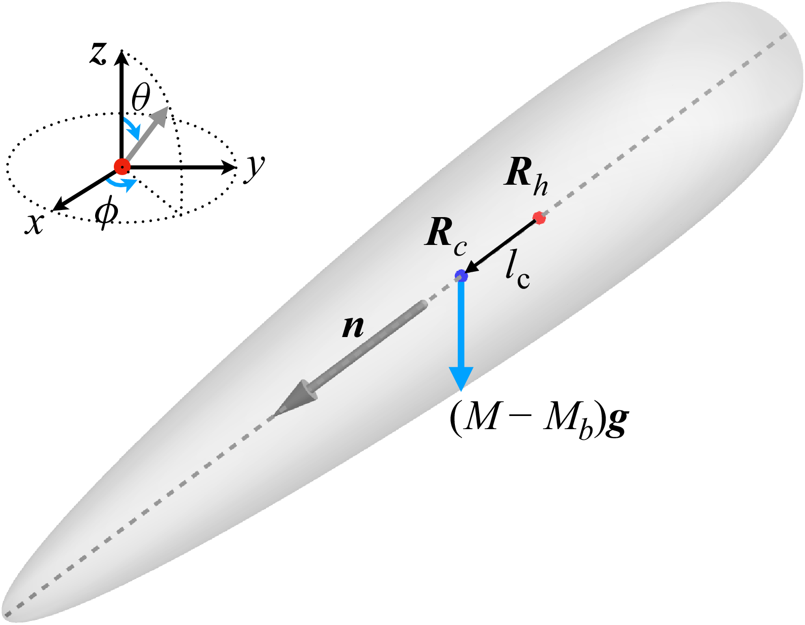
 Rh
Rh Rc
Rc n
n lc
lc Mg
Mg −Mbg
−Mbg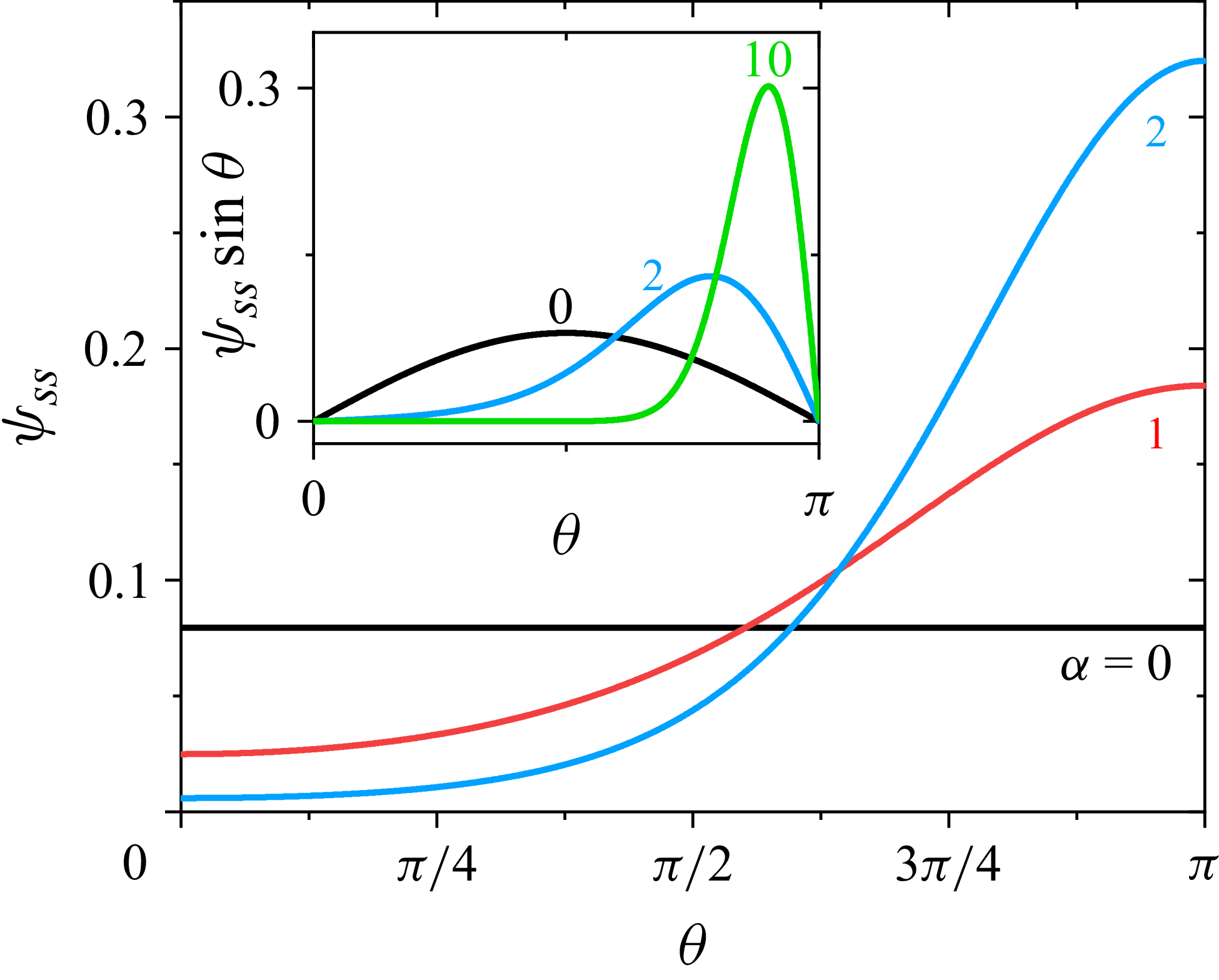
 ψss(θ,ϕ)
 sinθ
sinθ θ
θ
 uz
uz r
r α
α uz
uz α
α r
r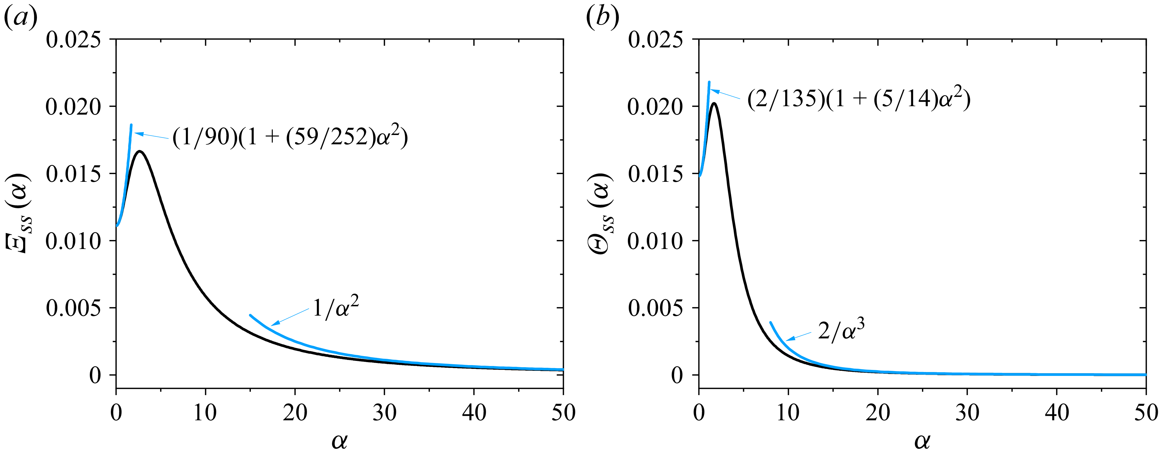
 Ξss(α)
 Θss(α)
 Dx-y
Dx-y Dz
Dz β0=(M−Mb)gL/(kBT)
 ϵ=lc/L
 β0
β0 Dx-y
Dx-y Dz
Dz ϵ
ϵ β0
β0
 Dx−y
Dx−y Dz
Dz r
r α=0
α=0 β0=(M−Mb)gL/(kBT)
 Dx−y
Dx−y Dz
Dz α
α Dmax
Dmax r
r β0
β0
 β
β α=0
α=0 r=10
r=10 τcross
 τr
τr α
α α
α 1/α=τo/τr
 Open access

