





1. Introduction
The onset of linear instability in the plane Poiseuille flow, particularly within the context of viscoelastic fluids overlying porous media, presents a multifaceted yet crucial area of investigation. While stability analyses of Newtonian flow in channels with porous walls have attracted considerable attention due to their relevance across various fields (Majdalani, Zhou & Dawson Reference Majdalani, Zhou and Dawson2002; Jiang et al. Reference Jiang, Yu, Sun and Wang2004; Bickerton, Govignon & Kelly Reference Bickerton, Govignon and Kelly2013; Berkowitz et al. Reference Berkowitz, Dror, Hansen and Scher2016), incorporating viscoelasticity introduces additional complexity that necessitates deeper exploration, with applications ranging from industrial processes to biomedical engineering. Instability analysis is pivotal in discerning the transition point flow regime, especially in scenarios where laminar-to-turbulent transition affects efficiency and performance. The insight gained from such investigations advances our fundamental understanding of fluid–porous media interactions and informs the design and optimization of a wide array of engineering systems (Skartsis, Khomami & Kardos Reference Skartsis, Khomami and Kardos1992; Talwar & Khomami Reference Talwar and Khomami1995; Khomami & Moreno Reference Khomami and Moreno1997). This study delves into the stability analysis of Oldroyd-B fluid within a plane Poiseuille flow confined by porous walls to elucidate the intricate interplay between fluid rheology and porous media characteristics on flow stability.
1.1. Stability in Newtonian channel flows overlying porous walls
Stability analysis of Newtonian flows with porous walls has received great attention numerically and experimentally due to its applications in various fields like filtration processes (Bickerton et al. Reference Bickerton, Govignon and Kelly2013), biological fluid (Majdalani et al. Reference Majdalani, Zhou and Dawson2002), sediment–water interfaces (Berkowitz et al. Reference Berkowitz, Dror, Hansen and Scher2016) and cooling systems of rocket engines (Jiang et al. Reference Jiang, Yu, Sun and Wang2004). While the laminar Newtonian flow in a pipe is linearly stable at all Reynolds numbers ( $ \textit{Re}$
), the Tollmien–Schlichting (TS) instability occurs in plane Poiseuille flow at
$ \textit{Re}$
), the Tollmien–Schlichting (TS) instability occurs in plane Poiseuille flow at $ \textit{Re} = 5772$
(Drazin & Reid Reference Drazin and Reid1981; Schmid, Henningson & Jankowski Reference Schmid, Henningson and Jankowski2002). Incorporating porous media into the channel significantly alters the fluid dynamics and impacts stability. Numerous experimental and computational studies have underscored the profound influence of porous materials on the flow physics and stability of Newtonian fluids within channels (Beavers & Joseph Reference Beavers and Joseph1967; Beavers, Sparrow & Magnuson Reference Beavers, Sparrow and Magnuson1970; Sparrow et al. Reference Sparrow, Beavers, Chen and Lloyd1973; Min & Kim Reference Min and Kim2005; Tilton & Cortelezzi Reference Tilton and Cortelezzi2006; Silin et al. Reference Silin, Converti, Dalponte and Clausse2011).
$ \textit{Re} = 5772$
(Drazin & Reid Reference Drazin and Reid1981; Schmid, Henningson & Jankowski Reference Schmid, Henningson and Jankowski2002). Incorporating porous media into the channel significantly alters the fluid dynamics and impacts stability. Numerous experimental and computational studies have underscored the profound influence of porous materials on the flow physics and stability of Newtonian fluids within channels (Beavers & Joseph Reference Beavers and Joseph1967; Beavers, Sparrow & Magnuson Reference Beavers, Sparrow and Magnuson1970; Sparrow et al. Reference Sparrow, Beavers, Chen and Lloyd1973; Min & Kim Reference Min and Kim2005; Tilton & Cortelezzi Reference Tilton and Cortelezzi2006; Silin et al. Reference Silin, Converti, Dalponte and Clausse2011).
The governing equations for porous media were first introduced by Darcy (Reference Darcy1856). Darcy’s law established a relationship between pressure drop and velocity within an unbounded porous medium, serving as a cornerstone for porous media flow modelling. However, Darcy’s law is limited in its applicability, as it neglects viscous transport effects and does not account for flow discontinuities at boundaries, making it invalid in regions where boundary effects are significant. To address these limitations, Brinkman (Reference Brinkman1949) extended Darcy’s model by incorporating viscous transport into the momentum balance equation, allowing velocities to be treated as dependent variables in various spatial directions. This modification, referred to as the Brinkman equation, provides a more comprehensive description of flow in porous media, particularly in cases where viscous shear effects cannot be ignored. Based on these developments, Beavers & Joseph (Reference Beavers and Joseph1967) formulated the first interface condition to model the interaction between a liquid and a porous medium, considering the slip velocity at the interface. Their interface condition, commonly known as the Beavers–Joseph condition, was later employed by Beavers et al. (Reference Beavers, Sparrow and Magnuson1970) in a study that was among the first to demonstrate the destabilizing effects of wall permeability on flow stability. Subsequently, Sparrow et al. (Reference Sparrow, Beavers, Chen and Lloyd1973) experimentally determined critical Reynolds numbers for a channel with a single porous wall and conducted a two-dimensional linear stability analysis using Darcy’s law in conjunction with the Beavers–Joseph interface condition. Their findings confirmed that wall permeability reduces the critical Reynolds number compared with flow in channels with impermeable walls, highlighting the destabilizing influence of porous boundaries.
A significant advancement in the modelling of porous media flow came with introducing the volume-averaged Navier–Stokes (VANS) equations by Whitaker (Reference Whitaker1996). Unlike previous models, which largely neglected inertial effects within porous media, the VANS equations incorporate additional terms to account for inertial contributions arising from the porous medium’s geometric structure and resistance function. This enhancement enables a more accurate representation of flow dynamics, particularly in high-velocity and high-porosity regimes (Tilton & Cortelezzi Reference Tilton and Cortelezzi2008). To bridge the Navier–Stokes equations governing the free-fluid region and the VANS equations governing the porous domain, Ochoa-Tapia & Whitaker (Reference Ochoa-Tapia and Whitaker1995a , Reference Ochoa-Tapia and Whitakerb ) and Alberto (Reference Alberto1998) introduced a set of momentum-transfer interface conditions. These conditions refine the shear stress balance at the interface, ensuring a more realistic representation of the momentum exchange between the fluid and the porous medium.
Later, Chang, Chen & Straughan (Reference Chang, Chen and Straughan2006) conducted one of the earliest detailed analyses by coupling the Navier–Stokes equations in the free-flow region with Darcy’s law in the porous layer through the Beavers & Joseph (Reference Beavers and Joseph1967) slip condition. Their results showed that the stability structure of the system can shift between bimodal and trimodal behaviour depending on the porous-layer properties, particularly its permeability and thickness. Building on these findings, Hill & Straughan (Reference Hill and Straughan2008) revisited the problem using the Darcy–Brinkman formulation, which incorporates viscous diffusion within the porous layer and provides a smoother transition at the interface in configurations with a single porous wall. Further advancements were made by Tilton & Cortelezzi (Reference Tilton and Cortelezzi2006), who applied Whitaker’s VANS (Whitaker Reference Whitaker1996) together with the momentum-transfer conditions of Ochoa-Tapia & Whitaker (Reference Ochoa-Tapia and Whitaker1995a
,
Reference Ochoa-Tapia and Whitakerb
). Their analysis showed that even modest wall permeability can destabilize the flow. A more systematic parametric study by Tilton & Cortelezzi (Reference Tilton and Cortelezzi2008) demonstrated that increasing permeability and decreasing porous-layer thickness lowers the critical Reynolds number, while increasing the interfacial shear-stress coefficient $\tau$
has a stabilizing effect due to enhanced momentum exchange and modified slip at the interface. More recently, Samanta (Reference Samanta2022) extended these investigations to inhomogeneous and anisotropic porous substrates, revealing that anisotropy can suppress classical shear instabilities and reduce non-modal disturbance amplification, thereby altering stability pathways in a fundamental way. Additional studies have explored related configurations (Liu & Liu Reference Liu and Liu2009; Wu & Mirbod Reference Wu and Mirbod2018, Reference Wu and Mirbod2019; Ghosh et al. Reference Ghosh, Loiseau, Breugem and Brandt2019; Samanta Reference Samanta2020; Hooshyar et al. Reference Hooshyar, Yoshikawa and Mirbod2022; Mirbod et al. Reference Mirbod, Abtahi, Bilondi, Rosti and Brandt2023, Reference Mirbod, Hooshyar, Taheri and Yoshikawa2024; Rosti, Mirbod & Brandt Reference Rosti, Mirbod and Brandt2021).
$\tau$
has a stabilizing effect due to enhanced momentum exchange and modified slip at the interface. More recently, Samanta (Reference Samanta2022) extended these investigations to inhomogeneous and anisotropic porous substrates, revealing that anisotropy can suppress classical shear instabilities and reduce non-modal disturbance amplification, thereby altering stability pathways in a fundamental way. Additional studies have explored related configurations (Liu & Liu Reference Liu and Liu2009; Wu & Mirbod Reference Wu and Mirbod2018, Reference Wu and Mirbod2019; Ghosh et al. Reference Ghosh, Loiseau, Breugem and Brandt2019; Samanta Reference Samanta2020; Hooshyar et al. Reference Hooshyar, Yoshikawa and Mirbod2022; Mirbod et al. Reference Mirbod, Abtahi, Bilondi, Rosti and Brandt2023, Reference Mirbod, Hooshyar, Taheri and Yoshikawa2024; Rosti, Mirbod & Brandt Reference Rosti, Mirbod and Brandt2021).
1.2. Stability of rectilinear viscoelastic shearing flow
Instability in viscoelastic channel flows has attracted significant interest due to its fundamental importance and broad industrial relevance, including applications in polymer processing, biomedical devices, enhanced oil recovery and food manufacturing (Larson Reference Larson1992; Kucharová et al. Reference Kucharová, Doubal, Klemera, Rejchrt and Navrátil2007; Baird & Collias Reference Baird and Collias2014; Ahmed & Basu Reference Ahmed and Basu2016; Hu et al. Reference Hu, Tang, Mpelwa, Jiang and Feng2021). Numerous experimental and numerical studies have shown that adding polymers to Newtonian flows can profoundly modify stability characteristics and influence the transition between flow regimes (Dubief, Terrapon & Soria Reference Dubief, Terrapon and Soria2013; Samanta et al. Reference Samanta, Dubief, Holzner, Schäfer, Morozov, Wagner and Hof2013; Srinivas & Kumaran Reference Srinivas and Kumaran2017; Choueiri, Lopez & Hof Reference Choueiri, Lopez and Hof2018; Chandra et al. Reference Chandra, Shankar and Das2018, Reference Chandra, Shankar and Das2020; Garg et al. Reference Garg, Chaudhary, Khalid, Shankar and Subramanian2018; Shekar et al. Reference Shekar, McMullen, Wang, McKeon and Graham2019; Khalid, Shankar & Subramanian Reference Khalid, Shankar and Subramanian2021b ).
Unlike Newtonian fluids, where instability primarily arises from fluid inertia, non-Newtonian fluids can experience instability driven by elasticity, even without significant inertia. These so-called elastic instabilities were first identified in Taylor–Couette flow, where shear thinning effects were negligible (Larson, Shaqfeh & Muller Reference Larson, Shaqfeh and Muller1990; Shaqfeh Reference Shaqfeh1996). Later, researchers discovered that elastic instabilities could also occur in other flow systems. At low inertia and high Weissenberg numbers, Sureshkumar et al. (Reference Sureshkumar, Smith, Armstrong and Brown1999) investigated the linear and nonlinear stability of viscoelastic fluids in both plane Couette flow and pressure-driven flow. Their analysis, based on the upper convected Maxwell (UCM) and Oldroyd-B constitutive models, highlighted the impact of elasticity on flow stability. In Poiseuille flow within the inertial regime, Sureshkumar & Beris (Reference Sureshkumar and Beris1995) demonstrated that elasticity significantly destabilizes UCM fluids. Building on this, Blonce (Reference Blonce1997) conducted a linear stability analysis for Giesekus fluids and found that elasticity destabilizes flows with Reynolds numbers of $O(10^3)$
.
$O(10^3)$
.
In an experimental study, Samanta et al. (Reference Samanta, Dubief, Holzner, Schäfer, Morozov, Wagner and Hof2013) discovered that at high polymer concentrations, a novel instability arises, triggering a transition from laminar to turbulent flow at significantly lower Reynolds numbers than in Newtonian fluids. This new flow regime, elasto-inertial turbulence, highlights the crucial interplay between fluid elasticity and inertia. Subsequent experiments further demonstrated that viscoelastic flow in pipes becomes unstable at Reynolds numbers as low as 800, far below the critical threshold for Newtonian turbulence (Chandra, Shankar & Das Reference Chandra, Shankar and Das2018; Choueiri et al. Reference Choueiri, Lopez and Hof2018; Chandra, Shankar & Das Reference Chandra, Shankar and Das2020). While most experimental studies on viscoelastic transitions have focused on pipe geometries, Srinivas & Kumaran (Reference Srinivas and Kumaran2017) extended this investigation to microchannel flows of dilute polymer solutions using particle image velocimetry measurements. Their study revealed that the transition occurred within a rectangular channel with a 160 μm gap width at Reynolds numbers between 100 and 300, a significantly lower threshold than Newtonian flows. These findings emphasize the profound impact of elasticity on flow stability, even in small-scale systems.
The eigenspectrum of Newtonian plane Couette, pipe and plane Poiseuille flows exhibits a characteristic ‘Y-shaped’ structure with wall, centre and highly damped branches. For plane Poiseuille flow, linear instability arises only beyond $ \textit{Re} = 5772$
through TS waves (Drazin & Reid Reference Drazin and Reid1981; Schmid et al. Reference Schmid, Henningson and Jankowski2002). Introducing elasticity substantially modifies this structure. Using the UCM model, Porteous & Denn (Reference Porteous and Denn1972) showed that viscoelastic Poiseuille flow can exhibit multiple unstable modes at high Reynolds numbers. The choice of constitutive model strongly influences stability predictions: Sureshkumar & Beris (Reference Sureshkumar and Beris1995) demonstrated that Oldroyd–B fluids are generally more stable than UCM fluids and that elasticity has a non-monotonic effect, initially reducing the critical Reynolds number but eventually stabilizing the flow at higher elasticity numbers. Further work by Zhang et al. (Reference Zhang, Lashgari, Zaki and Brandt2013) using Oldroyd–B and FENE-P (finite extensible nonlinear elastic–Peterlin) models revealed that instability is governed by the ratio of polymer relaxation time to the characteristic instability time scale – short relaxation times enhance both modal and non-modal growth, whereas longer relaxation times suppress disturbances.
$ \textit{Re} = 5772$
through TS waves (Drazin & Reid Reference Drazin and Reid1981; Schmid et al. Reference Schmid, Henningson and Jankowski2002). Introducing elasticity substantially modifies this structure. Using the UCM model, Porteous & Denn (Reference Porteous and Denn1972) showed that viscoelastic Poiseuille flow can exhibit multiple unstable modes at high Reynolds numbers. The choice of constitutive model strongly influences stability predictions: Sureshkumar & Beris (Reference Sureshkumar and Beris1995) demonstrated that Oldroyd–B fluids are generally more stable than UCM fluids and that elasticity has a non-monotonic effect, initially reducing the critical Reynolds number but eventually stabilizing the flow at higher elasticity numbers. Further work by Zhang et al. (Reference Zhang, Lashgari, Zaki and Brandt2013) using Oldroyd–B and FENE-P (finite extensible nonlinear elastic–Peterlin) models revealed that instability is governed by the ratio of polymer relaxation time to the characteristic instability time scale – short relaxation times enhance both modal and non-modal growth, whereas longer relaxation times suppress disturbances.
Recently, Garg et al. (Reference Garg, Chaudhary, Khalid, Shankar and Subramanian2018) identified a novel instability in the viscoelastic channel and pipe flows governed by the Oldroyd-B model. Unlike the classical TS instability in Newtonian plane Poiseuille flow, where disturbances are localized near the wall and associated with ‘wall modes’ (WM), their study revealed that the unstable modes in viscoelastic flows belong to the ‘centre modes,’ with phase speeds closely matching the maximum velocity of the base flow. In addition, as the Reynolds number ( $ \textit{Re}$
) increases, disturbances shift towards the pipe or channel centreline, highlighting a fundamental departure from Newtonian instability mechanisms. Expanding on these findings, Chaudhary et al. (Reference Chaudhary, Garg, Shankar and Subramanian2019) investigated wall-mode instabilities in plane Poiseuille and plane Couette flows of a UCM fluid. Their study uncovered a variety of new unstable modes arising from the combined effects of inertia and elasticity. Later, Chaudhary et al. (Reference Chaudhary, Garg, Subramanian and Shankar2021) conducted a comprehensive stability analysis of viscoelastic pressure-driven pipe flow using the Oldroyd-B model. Unlike conventional stability studies that examine instability along the
$ \textit{Re}$
) increases, disturbances shift towards the pipe or channel centreline, highlighting a fundamental departure from Newtonian instability mechanisms. Expanding on these findings, Chaudhary et al. (Reference Chaudhary, Garg, Shankar and Subramanian2019) investigated wall-mode instabilities in plane Poiseuille and plane Couette flows of a UCM fluid. Their study uncovered a variety of new unstable modes arising from the combined effects of inertia and elasticity. Later, Chaudhary et al. (Reference Chaudhary, Garg, Subramanian and Shankar2021) conducted a comprehensive stability analysis of viscoelastic pressure-driven pipe flow using the Oldroyd-B model. Unlike conventional stability studies that examine instability along the $ \textit{Wi}$
or
$ \textit{Wi}$
or $ \textit{Re}$
axes, they explored the three-dimensional
$ \textit{Re}$
axes, they explored the three-dimensional $ \textit{Re}- \textit{Wi}-\beta$
parameter space. They confirmed that both UCM and Oldroyd-B fluids remain stable at low Reynolds numbers. To establish the presence of similar centre-mode instabilities in channel flow, Khalid et al. (Reference Khalid, Chaudhary, Garg, Shankar and Subramanian2021a
) analysed the stability of plane Poiseuille flow with an Oldroyd-B fluid across a broad range of
$ \textit{Re}- \textit{Wi}-\beta$
parameter space. They confirmed that both UCM and Oldroyd-B fluids remain stable at low Reynolds numbers. To establish the presence of similar centre-mode instabilities in channel flow, Khalid et al. (Reference Khalid, Chaudhary, Garg, Shankar and Subramanian2021a
) analysed the stability of plane Poiseuille flow with an Oldroyd-B fluid across a broad range of $ \textit{Re}$
,
$ \textit{Re}$
, $ \textit{Wi}$
and
$ \textit{Wi}$
and $\beta$
. Their results confirmed the existence of instability at Reynolds numbers significantly lower than 1000, providing further insight into the similarities and differences between centre-mode instabilities in pipe and channel flows.
$\beta$
. Their results confirmed the existence of instability at Reynolds numbers significantly lower than 1000, providing further insight into the similarities and differences between centre-mode instabilities in pipe and channel flows.
More recently, Yadav, Subramanian & Shankar (Reference Yadav, Subramanian and Shankar2024) examined the linear stability of viscoelastic channel flows within the Couette–Poiseuille flow. Their study aimed to identify parameter regimes where viscoelastic Couette–Poiseuille flow exhibits instability in the inertialess limit, providing new perspectives on elastic instabilities. Additional investigations into the stability of channel and pipe flows can be found in Shekar et al. (Reference Shekar, McMullen, Wang, McKeon and Graham2019, Reference Shekar, McMullen, McKeon and Graham2020) and Page, Dubief & Kerswell (Reference Page, Dubief and Kerswell2020), further advancing the understanding of viscoelastic flow instabilities across different geometries and flow conditions.
1.3. Stability of viscoelastic flows with porous media
The dynamics of viscoelastic fluids in porous media have attracted significant attention across various disciplines, including biorheology, geophysics and the chemical and petroleum industries. In environmental and geophysical contexts, such flows are relevant to water–soil interactions and the transport of crude oil through fractured formations. Many of these scenarios involve non-Newtonian fluids, such as lava and mudflows, which exhibit both viscous and elastic properties (Khuzhayorov, Auriault & Royer Reference Khuzhayorov, Auriault and Royer2000; Khaled & Vafai Reference Khaled and Vafai2003; Joseph Reference Joseph2013; Tierra et al. Reference Tierra, Pavissich, Nerenberg, Xu and Alber2015). As discussed in the previous section, viscoelastic fluids exhibit complex rheological behaviour due to their combined elastic and viscous properties. When these fluids interact with a porous structure, the resulting flow dynamics become even more intricate due to additional constraints imposed by the pore geometry and solid–fluid interactions (Zami-Pierre et al. Reference Zami-Pierre, De Loubens, Quintard and Davit2016; De et al. Reference De, Krishnan, Van Der Schaaf, Kuipers, Peters and Padding2018b ; Kumar & Ardekani Reference Kumar and Ardekani2021).
While the stability of viscoelastic fluids in porous media has received increasing attention in recent years, the development of macroscopic mathematical models for such flows remains relatively underdeveloped compared with their Newtonian counterparts. This disparity has constrained progress in understanding and predicting the complex behaviour of viscoelastic fluids in porous structures. A detailed review of constitutive equations governing non-Newtonian fluid flow in porous media is provided by Rudraiah & Kaloni (Reference Rudraiah and Kaloni1990). Among the earliest attempts to formulate a macroscopic model for viscoelastic flow in porous media is the work of Alishaev & Mirzadjanzade (Reference Alishaev and Mirzadjanzade1975), who derived a pressure–velocity relationship for Oldroyd-B fluids, resulting in what is now referred to as the modified Darcy–Oldroyd-B model. This framework has since served as a foundation for investigating thermal instabilities in viscoelastic flows. For example, Kim et al. (Reference Kim, Lee, Kim and Chung2003) analysed the onset of thermal convection in a porous medium saturated with an Oldroyd-B fluid, using the modified Darcy–Oldroyd model to determine critical conditions for instability. Raghunatha et al. (Reference Raghunatha and Shivakumara2018) later extended this approach to examine the nonlinear stability of thermal convection, incorporating anisotropic permeability and thermal diffusivity effects.
Despite its utility, the classical Darcy-based models are limited in their applicability due to their neglect of boundary layer effects, rendering them appropriate primarily for unbounded or idealized porous domains. To address this limitation, Tan & Masuoka (Reference Tan and Masuoka2005) introduced an improved formulation for Stokes’ first problem in a porous half-space by incorporating the extra stress tensor using a local volume averaging technique (Vafai & Tien Reference Vafai and Tien1981; Masuoka & Takatsu Reference Masuoka and Takatsu2002). This enhanced model more accurately captures boundary effects in viscoelastic flows, as illustrated by Zhang, Fu & Tan (Reference Zhang, Fu and Tan2008) in their linear and nonlinear stability analyses of thermal convection in an Oldroyd-B fluid-saturated porous layer. Building on this refinement, more general models such as the modified Darcy–Brinkman–Maxwell and Darcy–Brinkman–Oldroyd formulations have been developed to incorporate both boundary-layer and viscous effects, making them suitable for highly porous or confined geometries. Tan & Masuoka (Reference Tan and Masuoka2007), for instance, employed the Darcy–Brinkman–Maxwell model to examine thermoconvective instability in a Maxwell fluid under bottom heating, while Sun et al. (Reference Sun, Wang, Zhao, Yin and Zhang2019) investigated chaotic convection in Oldroyd-B fluids under periodic thermal forcing via the Oldroyd-B model.
In a recent study, Song & Ding (Reference Song and Ding2023) investigated the linear stability of an Oldroyd-B liquid film flowing down an inclined porous substrate, incorporating the Darcy equation with classical Beavers–Joseph boundary conditions at the fluid–porous interface. It should be noted that within the porous layer, they considered a Newtonian fluid for simplification of their model. Experimental studies have provided valuable insight into viscoelastic flow behaviour in porous structures, from early investigations around isolated or periodic cylinders (Skartsis et al. Reference Skartsis, Khomami and Kardos1992; Talwar & Khomami Reference Talwar and Khomami1995; Khomami & Moreno Reference Khomami and Moreno1997) to more recent microfluidic experiments (Moss & Rothstein Reference Moss and Rothstein2010; Galindo-Rosales et al. Reference Galindo-Rosales, Campo-Deano, Pinho, Van Bokhorst, Hamersma, Oliveira and Alves2012). Using micropost arrays, Walkama, Waisbord & Guasto (Reference Walkama, Waisbord and Guasto2020) showed that geometric disorder can suppress chaotic fluctuations, whereas Haward, Hopkins & Shen (Reference Haward, Hopkins and Shen2021) reported that slight disorder may instead enhance them, depending on the distribution of stagnation points. Additional observations on pore-scale unsteadiness, instability onset and the influence of geometry are provided by De et al. (Reference De, Koesen, Maitri, Golombok, Padding and van Santvoort2018a ); Ibezim, Poole & Dennis (Reference Ibezim, Poole and Dennis2021) and Ibezim, Dennis & Poole (Reference Ibezim, Dennis and Poole2024).
Numerical approaches have likewise evolved, ranging from generalized Darcy-type continuum models (Pearson & Tardy Reference Pearson and Tardy2002) and pore-network formulations (Sochi Reference Sochi2010) to direct simulations of viscoelastic flow through idealized porous structures (Skartsis et al. Reference Skartsis, Khomami and Kardos1992; Liu et al. Reference Liu, Bornside, Armstrong and Brown1998). More advanced methods, such as the coupled finite-volume/immersed-boundary framework of De et al. (Reference De, Kuipers, Peters and Padding2017), further highlight how pore geometry and symmetry strongly influence flow organization and the onset of instability. Pore-scale viscoelastic instabilities have also been examined numerically. Using the FENE-P model, Kumar et al. (Reference Kumar, Aramideh, Browne, Datta and Ardekani2021) showed that increasing the Weissenberg number shifts porous-channel flow from boundary vortices to multiple vortical structures. Kumar & Ardekani (Reference Kumar and Ardekani2021) identified distinct instability regimes between two closely spaced cylinders driven by polymeric stress distributions, while Kumar & Ardekani (Reference Kumar and Ardekani2023) demonstrated that geometric asymmetry produces uneven flow patterns and eddies at intermediate Weissenberg numbers. Additional related studies include Gillissen (Reference Gillissen2013), De et al. (Reference De, Das, Kuipers, Peters and Padding2016) and Aramideh, Vlachos & Ardekani (Reference Aramideh, Vlachos and Ardekani2019). Nevertheless, the stability of pressure-driven viscoelastic channel flow interacting with porous walls remains insufficiently understood.
1.4. Aims of the current investigation
This study aims to address a critical gap in the stability analysis of pressure-driven viscoelastic channel flows with porous walls. While prior research has focused mainly on the convective instability of Oldroyd-B fluids inside porous media, limited attention has been given to pressure-driven flows involving free-flow and porous regions, particularly the influence of fluid–porous interfaces on flow physics and stability. Most existing studies have considered fully saturated porous media, thereby neglecting the role of fluid–porous interactions in modifying the flow stability characteristics. To bridge this gap, we perform a linear stability analysis of pressure-driven flow in a channel with rigid, homogeneous, isotropic, porous layers at the top and bottom walls. Our model couples the Oldroyd-B equations in the free-flow region with a modified Darcy–Brinkman–Oldroyd-B model (Tan & Masuoka Reference Tan and Masuoka2005) in the porous domain, incorporating key modifications and generalized boundary conditions to capture fluid–porous interactions accurately. We systematically investigate the influence of key parameters on the linear stability of viscoelastic channel flows with porous walls. The parameters of interest include the Weissenberg number ( $ \textit{Wi}$
) and the viscosity ratio (
$ \textit{Wi}$
) and the viscosity ratio ( $\beta$
) of the viscoelastic fluid, along with the permeability parameter (
$\beta$
) of the viscoelastic fluid, along with the permeability parameter ( $\alpha$
). While the momentum transfer coefficient at the fluid–porous interface,
$\alpha$
). While the momentum transfer coefficient at the fluid–porous interface, $\tau$
, plays a potentially significant role in interfacial dynamics, it is set to zero throughout this study. This simplification is motivated by the limited experimental data available on
$\tau$
, plays a potentially significant role in interfacial dynamics, it is set to zero throughout this study. This simplification is motivated by the limited experimental data available on $\tau$
in viscoelastic flows, leaving its influence an open question for future investigation. The porosity is fixed at
$\tau$
in viscoelastic flows, leaving its influence an open question for future investigation. The porosity is fixed at $\epsilon = 0.6$
, the porous layer thickness at
$\epsilon = 0.6$
, the porous layer thickness at $\delta =1$
, and the interfacial coupling at
$\delta =1$
, and the interfacial coupling at $\tau = 0$
.
$\tau = 0$
.
The paper is organized as follows. Section 2 presents the formulation of the problem, including the governing equations for the Oldroyd-B fluid, the boundary conditions and the linearization procedure. This section also includes a description of the numerical method and model validation. Sections 3.1 and 3.2 examine the eigenspectrum structure under various flow conditions. We begin with the Newtonian case, with and without porous boundaries, and then analyse the viscoelastic case for both smooth- and porous-walled channels. Particular attention is given to the emergence of a new unstable WM at high $ \textit{Wi}$
in high permeability. Section 3.3 focuses on the evolution of neutral stability curves with increasing
$ \textit{Wi}$
in high permeability. Section 3.3 focuses on the evolution of neutral stability curves with increasing $ \textit{Wi}$
at fixed
$ \textit{Wi}$
at fixed $\beta$
and varying
$\beta$
and varying $\alpha$
, while § 3.4 investigates the effect of varying
$\alpha$
, while § 3.4 investigates the effect of varying $\beta$
in porous-walled channels, including comparisons with impermeable cases. Section 3.5 concludes by comparing our numerical results with available experimental data.
$\beta$
in porous-walled channels, including comparisons with impermeable cases. Section 3.5 concludes by comparing our numerical results with available experimental data.
2. Problem formulation and mathematical model
2.1. Governing equations
Schematic diagram of the computational domain and coordinate systems.

We study pressure-driven flow of an incompressible viscoelastic fluid characterized by a constant density $\rho$
and total viscosity
$\rho$
and total viscosity $\mu$
(the sum of solvent
$\mu$
(the sum of solvent $\mu _{s}$
and polymer viscosity
$\mu _{s}$
and polymer viscosity $\mu _{p}$
) confined between two rigid, homogenous and isotropic porous layers. The gap in the free fluid region is
$\mu _{p}$
) confined between two rigid, homogenous and isotropic porous layers. The gap in the free fluid region is $2L$
, while the porous layers have a thickness of
$2L$
, while the porous layers have a thickness of $H$
, a porosity of
$H$
, a porosity of $\epsilon$
and a permeability of
$\epsilon$
and a permeability of $\kappa$
as illustrated in figure 1. To model the viscoelastic fluid, we employed the Oldroyd-B model, with
$\kappa$
as illustrated in figure 1. To model the viscoelastic fluid, we employed the Oldroyd-B model, with $\lambda _1$
representing the relaxation time of stress and
$\lambda _1$
representing the relaxation time of stress and $\lambda _2$
signifying the retardation time of deformation. The Oldroyd-B model used in this study is extensively employed for analysing elastic phenomena in dilute polymer solutions and describes polymer chains as non-interacting Hookean dumbbells (Larson Reference Larson2013). Past studies have successfully applied this model to analyse flow instabilities in various geometries (Sureshkumar & Beris Reference Sureshkumar and Beris1995; Shaqfeh Reference Shaqfeh1996; Morozov & van Saarloos Reference Morozov and van Saarloo2007; Zhang et al. Reference Zhang, Lashgari, Zaki and Brandt2013; Garg et al. Reference Garg, Chaudhary, Khalid, Shankar and Subramanian2018). We non-dimensionalized the governing equations by introducing several non-dimensional parameters as the Reynolds number (
$\lambda _2$
signifying the retardation time of deformation. The Oldroyd-B model used in this study is extensively employed for analysing elastic phenomena in dilute polymer solutions and describes polymer chains as non-interacting Hookean dumbbells (Larson Reference Larson2013). Past studies have successfully applied this model to analyse flow instabilities in various geometries (Sureshkumar & Beris Reference Sureshkumar and Beris1995; Shaqfeh Reference Shaqfeh1996; Morozov & van Saarloos Reference Morozov and van Saarloo2007; Zhang et al. Reference Zhang, Lashgari, Zaki and Brandt2013; Garg et al. Reference Garg, Chaudhary, Khalid, Shankar and Subramanian2018). We non-dimensionalized the governing equations by introducing several non-dimensional parameters as the Reynolds number ( $ \textit{Re}$
), the Weissenberg number (
$ \textit{Re}$
), the Weissenberg number ( $ \textit{Wi}$
), the ratio of solvent to total viscosity (
$ \textit{Wi}$
), the ratio of solvent to total viscosity ( $\beta$
), the permeability parameter (
$\beta$
), the permeability parameter ( $\alpha$
) and the ratio of porous thickness to half-width of the channel in free flow (
$\alpha$
) and the ratio of porous thickness to half-width of the channel in free flow ( $\delta$
). These parameters are defined as follows:
$\delta$
). These parameters are defined as follows: $ \textit{Re}={\rho U_{\textit{max}} L}/{\mu }$
,
$ \textit{Re}={\rho U_{\textit{max}} L}/{\mu }$
, $ \textit{Wi}={\lambda _1 U_{\textit{max}}}/{L}$
,
$ \textit{Wi}={\lambda _1 U_{\textit{max}}}/{L}$
, $\beta ={\mu _s}/{\mu }={\lambda _2}/{\lambda _1}$
,
$\beta ={\mu _s}/{\mu }={\lambda _2}/{\lambda _1}$
, $\alpha = {L}/{\sqrt {\kappa }}$
and
$\alpha = {L}/{\sqrt {\kappa }}$
and $\delta ={H}/{L}$
. Here,
$\delta ={H}/{L}$
. Here, $U_{\textit{max}}$
represents the maximum base state velocity. It should be noted, here,
$U_{\textit{max}}$
represents the maximum base state velocity. It should be noted, here, $\kappa$
denotes the intrinsic permeability of the porous medium, while the parameter
$\kappa$
denotes the intrinsic permeability of the porous medium, while the parameter $\alpha = L/\sqrt {\kappa }$
serves as its non-dimensional representation in the stability analysis. Thus,
$\alpha = L/\sqrt {\kappa }$
serves as its non-dimensional representation in the stability analysis. Thus, $\alpha$
varies inversely with the physical permeability: increasing
$\alpha$
varies inversely with the physical permeability: increasing $\kappa$
(a more permeable medium) corresponds to a smaller
$\kappa$
(a more permeable medium) corresponds to a smaller $\alpha$
, whereas decreasing
$\alpha$
, whereas decreasing $\kappa$
(a less permeable medium) yields a larger
$\kappa$
(a less permeable medium) yields a larger $\alpha$
. The non-dimensional continuity and momentum equations of the free flow region are given by
$\alpha$
. The non-dimensional continuity and momentum equations of the free flow region are given by
 \begin{align} \boldsymbol{\nabla }\boldsymbol{\cdot }\boldsymbol{u}=0, \\[-28pt] \nonumber \end{align}
 \begin{align} Re\left(\frac {\partial \boldsymbol{u}}{\partial t}+\boldsymbol{u}\boldsymbol{\cdot }\boldsymbol{\nabla }\boldsymbol{u}\right)=-\boldsymbol{\nabla } p+\boldsymbol{\nabla }\boldsymbol{\cdot }\boldsymbol{\tau }, \\[0pt] \nonumber \end{align}
where $\boldsymbol{u}=u_x\boldsymbol{e}_x+u_y\boldsymbol{e}_y$
represents the velocity profile and
$\boldsymbol{u}=u_x\boldsymbol{e}_x+u_y\boldsymbol{e}_y$
represents the velocity profile and $p$
indicates the pressure field in the free flow region. The total stress tensor is
$p$
indicates the pressure field in the free flow region. The total stress tensor is $\boldsymbol{\tau }=\boldsymbol{\tau }_s+\boldsymbol{\tau }_p$
where encompassing both Newtonian stress (
$\boldsymbol{\tau }=\boldsymbol{\tau }_s+\boldsymbol{\tau }_p$
where encompassing both Newtonian stress ( $\boldsymbol{\tau }_s$
) and polymer stress (
$\boldsymbol{\tau }_s$
) and polymer stress ( $\boldsymbol{\tau }_p$
) resulting from the presence of polymer additives. To model the relationship between the polymer stress and strain
$\boldsymbol{\tau }_p$
) resulting from the presence of polymer additives. To model the relationship between the polymer stress and strain $(\boldsymbol{D}= {\boldsymbol{\nabla }\boldsymbol{u}+\boldsymbol{\nabla }\boldsymbol{u}^T}/{2})$
, various models such as the Maxwell, Waters-B, FENE-P and Oldroyd-B models have been introduced (Bird, Armstrong & Hassager Reference Bird, Armstrong and Hassager1987; Joseph Reference Joseph2013; Larson Reference Larson2013; Morozov & Spagnolie Reference Morozov and Spagnolie2014). For the Oldroyd-B model that we used in this study, the non-dimensional constitutive relation between total stress and strain (Joseph Reference Joseph2013; Song & Ding Reference Song and Ding2023) is described as follows:
$(\boldsymbol{D}= {\boldsymbol{\nabla }\boldsymbol{u}+\boldsymbol{\nabla }\boldsymbol{u}^T}/{2})$
, various models such as the Maxwell, Waters-B, FENE-P and Oldroyd-B models have been introduced (Bird, Armstrong & Hassager Reference Bird, Armstrong and Hassager1987; Joseph Reference Joseph2013; Larson Reference Larson2013; Morozov & Spagnolie Reference Morozov and Spagnolie2014). For the Oldroyd-B model that we used in this study, the non-dimensional constitutive relation between total stress and strain (Joseph Reference Joseph2013; Song & Ding Reference Song and Ding2023) is described as follows:
 \begin{align} \boldsymbol{\tau } + \textit{Wi} \overset {\boldsymbol{\nabla }}{\boldsymbol{\tau }}=2 \left(\boldsymbol{D}+ \textit{Wi}\beta \overset {\boldsymbol{\nabla }}{\boldsymbol{D}} \right)\!. \end{align}
Here, the superscript sign of $\boldsymbol{\nabla}$
is the upper convective derivative (
$\boldsymbol{\nabla}$
is the upper convective derivative ( $\overset {\boldsymbol{\nabla }}{\bullet })={\partial (\bullet )}/{\partial t}+u\boldsymbol{\cdot }\boldsymbol{\nabla }(\bullet ) - (\boldsymbol{\nabla }u)^T\boldsymbol{\cdot }(\bullet )-(\bullet )\boldsymbol{\cdot }\boldsymbol{\nabla }u$
).
$\overset {\boldsymbol{\nabla }}{\bullet })={\partial (\bullet )}/{\partial t}+u\boldsymbol{\cdot }\boldsymbol{\nabla }(\bullet ) - (\boldsymbol{\nabla }u)^T\boldsymbol{\cdot }(\bullet )-(\bullet )\boldsymbol{\cdot }\boldsymbol{\nabla }u$
).
In the porous region, the flow is modelled using the generalized form of the modified Darcy–Brinkman–Oldroyd-B equations initially proposed by Tan & Masuoka (Reference Tan and Masuoka2005), which retain the full stress–strain coupling and momentum transport terms. However, their analysis invoked several simplifying assumptions, including unidirectional flow, the absence of pressure gradients, and a reduced treatment of viscous stress terms for Stokes’ first problem of an Oldroyd-B in a porous half-space. In contrast, the present work employs the full form of the modified Darcy–Brinkman–Oldroyd-B model, retaining all relevant terms in the momentum and constitutive equations. Specifically, we preserve the complete viscous stress divergence term, $\boldsymbol{\nabla }\boldsymbol{\cdot }\boldsymbol{\tau }_{m,j}$
, and evaluate it using the Oldroyd-B constitutive relation; thereby, capturing the full interplay between elastic stresses and velocity gradients within the porous layer. This formulation enables a rigorous coupling between the viscoelastic free-flow region and the porous region, accurately resolving interfacial dynamics without the need for artificial boundary conditions.
$\boldsymbol{\nabla }\boldsymbol{\cdot }\boldsymbol{\tau }_{m,j}$
, and evaluate it using the Oldroyd-B constitutive relation; thereby, capturing the full interplay between elastic stresses and velocity gradients within the porous layer. This formulation enables a rigorous coupling between the viscoelastic free-flow region and the porous region, accurately resolving interfacial dynamics without the need for artificial boundary conditions.
Moreover, our model is applicable to both steady and unsteady flows of viscoelastic fluids through isotropic, homogeneous and rigid porous media. Thus, by using the generalized form of modified Darcy–Brinkman–Oldroyd-B model (Appendix A), the governing equations for mass and momentum conservation in the porous region are written in their fully generalized form, capable of capturing transient and nonlinear effects arising from the viscoelastic nature of the fluid as
 \begin{align} \boldsymbol{\nabla }\boldsymbol{\cdot }\boldsymbol{u}_{m,j}=0,\quad j=1,2 \\[-28pt] \nonumber \end{align}
 \begin{align} Re\left(1+ \textit{Wi} \frac {\partial }{\partial t}\right)\frac {\text{d}\boldsymbol{u}_{m,j}}{\text{d}t} & =-\epsilon \left(1+\textit{Wi} \frac {\partial }{\partial t}\right)\boldsymbol{\nabla } p_{m,j} +\left(1+\textit{Wi}\beta \frac {\partial }{\partial t}\right)\boldsymbol{\nabla }\boldsymbol{\cdot }\boldsymbol{\tau }_{m,j} \nonumber \\ & \quad - \epsilon \alpha ^2\left(1+\textit{Wi}\beta \frac {\partial }{\partial t}\right)\boldsymbol{u}_{m,j}. \\[0pt] \nonumber \end{align}
In the porous regions, the velocity, pressure and total stress tensor of the viscoelastic fluid are denoted by $\boldsymbol{u}_{m,j}=u_{x_{m,j}}\boldsymbol{e}_x+{u}=u_{y_{m,j}}\boldsymbol{e}_y$
,
$\boldsymbol{u}_{m,j}=u_{x_{m,j}}\boldsymbol{e}_x+{u}=u_{y_{m,j}}\boldsymbol{e}_y$
, $p_{m,j}$
and
$p_{m,j}$
and $\tau _{m,j}$
, respectively, where the subscript
$\tau _{m,j}$
, respectively, where the subscript $m$
indicates quantities associated with the porous medium. The additional subscript
$m$
indicates quantities associated with the porous medium. The additional subscript $j=1,2$
distinguishes between the channel’s upper (
$j=1,2$
distinguishes between the channel’s upper ( $j=1$
) and lower (
$j=1$
) and lower ( $j=2$
) porous layers. To describe the viscoelastic stress within the porous regions, we adopt the Oldroyd-B constitutive relation, which relates the total stress (
$j=2$
) porous layers. To describe the viscoelastic stress within the porous regions, we adopt the Oldroyd-B constitutive relation, which relates the total stress ( $\tau _{m,j}$
) to the strain rate tensor (
$\tau _{m,j}$
) to the strain rate tensor ( ${D}_{m,j}$
), defined as
${D}_{m,j}$
), defined as $\boldsymbol{D}_{m,j}={\boldsymbol{\nabla }\boldsymbol{u}_{m,j}+\boldsymbol{\nabla }\boldsymbol{u}_{m,j}^T}/{2}$
. Following the approach of Wu & Mirbod (Reference Wu and Mirbod2019), we modify the standard constitutive model by replacing the total viscosity
$\boldsymbol{D}_{m,j}={\boldsymbol{\nabla }\boldsymbol{u}_{m,j}+\boldsymbol{\nabla }\boldsymbol{u}_{m,j}^T}/{2}$
. Following the approach of Wu & Mirbod (Reference Wu and Mirbod2019), we modify the standard constitutive model by replacing the total viscosity $\mu$
with an effective viscosity
$\mu$
with an effective viscosity ${\mu }/{\epsilon }$
, which accounts for the porosity
${\mu }/{\epsilon }$
, which accounts for the porosity $\epsilon$
of the medium and represents enhanced resistance to flow due to the porous media. As a result, the non-dimensionalized constitutive equation in the porous region takes the form
$\epsilon$
of the medium and represents enhanced resistance to flow due to the porous media. As a result, the non-dimensionalized constitutive equation in the porous region takes the form
 \begin{align} \boldsymbol{\tau }_{m,j}+\textit{Wi}\overset {\boldsymbol{\nabla }}{\boldsymbol{\tau }}_{{m,j}}=\frac {2}{\epsilon } \left(\boldsymbol{D}_{m,j}+\beta \textit{Wi} \overset {\boldsymbol{\nabla }}{\boldsymbol{D}}_{m,j}\right) \!. \end{align}
At the solid boundaries located at the top and bottom walls of the channel, we impose the standard no-slip and no-penetration boundary conditions. Accordingly, both velocity components vanish at the walls, such that
 \begin{align} \boldsymbol{u}_{m,1} = 0, \quad y = 1+\delta ; \qquad \boldsymbol{u}_{m,2} = 0, \quad y = -(1+\delta ). \end{align}
At the interfaces between the free-flow and porous regions, we impose continuity of velocity, normal stress and shear stress to ensure smooth coupling between the two domains. In this work, we adopt a zero momentum-transfer coefficient, $\tau = 0$
, to isolate the fundamental effects of viscoelasticity and wall permeability on flow stability. Introducing a non-zero
$\tau = 0$
, to isolate the fundamental effects of viscoelasticity and wall permeability on flow stability. Introducing a non-zero $\tau$
would expand the parameter space and introduce additional interfacial coupling mechanisms that are beyond the scope of the present study. Physically,
$\tau$
would expand the parameter space and introduce additional interfacial coupling mechanisms that are beyond the scope of the present study. Physically, $\tau$
governs the shear-stress jump across a permeable interface, with
$\tau$
governs the shear-stress jump across a permeable interface, with $\tau = 0$
corresponding to a fully coupled interface in which the shear stress remains continuous. Realistic values of
$\tau = 0$
corresponding to a fully coupled interface in which the shear stress remains continuous. Realistic values of $\tau$
depend on the microstructure of the porous medium and typically require experimental characterization, and existing studies primarily address Newtonian flows. For Newtonian cases, the influence of
$\tau$
depend on the microstructure of the porous medium and typically require experimental characterization, and existing studies primarily address Newtonian flows. For Newtonian cases, the influence of $\tau$
on interfacial slip and stability has been examined in our previous work (Mirbod et al. Reference Mirbod, Hooshyar, Taheri and Yoshikawa2024) and in a work by Tilton & Cortelezzi (Reference Tilton and Cortelezzi2008), where its role in modifying stress balance and flow structure is demonstrated. Moreover, we employ the general expressions for stress derived directly from the governing equations in both regions. Since the streamwise normal stress exhibits minimal variation in streamwise direction, its contribution to the interfacial stress balance is neglected for simplification. Therefore, the interfacial boundary conditions at the junctions between the free-flow and porous layers are given by
$\tau$
on interfacial slip and stability has been examined in our previous work (Mirbod et al. Reference Mirbod, Hooshyar, Taheri and Yoshikawa2024) and in a work by Tilton & Cortelezzi (Reference Tilton and Cortelezzi2008), where its role in modifying stress balance and flow structure is demonstrated. Moreover, we employ the general expressions for stress derived directly from the governing equations in both regions. Since the streamwise normal stress exhibits minimal variation in streamwise direction, its contribution to the interfacial stress balance is neglected for simplification. Therefore, the interfacial boundary conditions at the junctions between the free-flow and porous layers are given by
 \begin{align} \boldsymbol{u}_{m,1} = \boldsymbol{u}, \quad {\tau _{yym,1}}-p_{m,1}={\tau _{yy}}-p,\qquad \tau _{xym,1}=\tau _{xy}, \qquad y = 1, \\[-28pt] \nonumber \end{align}
 \begin{align} \boldsymbol{u}_{m,2} = \boldsymbol{u}, \quad \tau _{yym,2}-p_{m,2}=\tau _{yy}-p,\qquad \tau _{xym,2}=\tau _{xy}, \qquad y = -1. \\[0pt] \nonumber \end{align}
2.2. The base state
In the steady, fully developed, pressure-driven channel flow of an Oldroyd-B fluid with porous walls, the base state velocity profile in the free flow region is unidirectional and identical to that of plane Poiseuille flow of a Newtonian fluid overlying porous walls. In this scenario, the nonlinear terms of the Oldroyd-B model do not influence the base velocity profile. The non-dimensional base velocity for the free flow is then given by
 \begin{align} \overline {\boldsymbol{u}} = \left [ \begin{array}{c} U(y) \\[4pt] 0 \\[4pt] 0 \\ \end{array} \right ], \end{align}
where $U(y) = C-y^2$
, with
$U(y) = C-y^2$
, with $C$
being a coefficient as a function of permeability parameter, porosity, and depth ratio. The equation details are provided in Appendix A. Here, the overbar symbols denote base-state quantities. However, the dimensionless base-state stress tensor differs from its Newtonian counterpart. The factor
$C$
being a coefficient as a function of permeability parameter, porosity, and depth ratio. The equation details are provided in Appendix A. Here, the overbar symbols denote base-state quantities. However, the dimensionless base-state stress tensor differs from its Newtonian counterpart. The factor $(1-\beta )$
appears due to the non-dimensionalization of the Oldroyd-B constitutive equation using the total viscosity, such that the polymeric stress scales with the polymer-to-total viscosity ratio. Unlike the Newtonian case, the viscoelastic base state contains a non-zero first normal stress difference, giving rise to the
$(1-\beta )$
appears due to the non-dimensionalization of the Oldroyd-B constitutive equation using the total viscosity, such that the polymeric stress scales with the polymer-to-total viscosity ratio. Unlike the Newtonian case, the viscoelastic base state contains a non-zero first normal stress difference, giving rise to the $\tau _{xx}$
component is defined as
$\tau _{xx}$
component is defined as
 \begin{align} \overline {\boldsymbol{\tau }} = \left [ \begin{array}{ccc} \bar {\tau }_{xx} & \bar {\tau }_{xy} & 0 \\[4pt] \bar {\tau }_{yx} & \bar {\tau }_{yy} & 0 \\[4pt] 0 & 0 & 0 \end{array} \right ] = \left [ \begin{array}{ccc} 2\textit{Wi}\left (\dfrac{\partial U}{\partial y}\right )^2(1 - \beta ) & \dfrac{\partial U}{\partial y} & 0 \\[12pt] \dfrac{\partial U}{\partial y} & 0 & 0 \\[12pt] 0 & 0 & 0 \end{array} \right ]. \end{align}
By solving the equations in the porous layers, we determined that the base velocity profile within these layers is also unidirectional. Moreover, the general forms of the base stress tensor are similar to those of the free flow layer, the main distinction being the inclusion of a $1/\epsilon$
coefficient for each term in the stress tensor. The dimensionless base-state velocity and stress tensor in the porous regions are expressed as
$1/\epsilon$
coefficient for each term in the stress tensor. The dimensionless base-state velocity and stress tensor in the porous regions are expressed as
 \begin{align} \overline {\boldsymbol{u}}_{m,j} = \left [ \begin{array}{ccc} U_{m,j}(y) \\[4pt] \displaystyle 0 \\[4pt] 0 \\ \end{array} \right ], \\[-28pt] \nonumber \end{align}
 \begin{align} \overline {\boldsymbol{\tau }}_{m,j} = \left [ \begin{array}{ccc} \bar {\tau }_{xx_{m,j}} & \bar {\tau }_{xy_{m,j}} & 0 \\[4pt] \displaystyle \bar {\tau }_{yx_{m,j}} & \bar {\tau }_{yy_{m,j}} & 0 \\[4pt] \displaystyle 0 & 0 & 0 \end{array} \right ]=\left [ \begin{array}{ccc} 2 {\textit{Wi}}/{\epsilon } \left(\dfrac{\partial U_{m,j}}{\partial y} \right)^2(1-\beta ) & \frac {1}{\epsilon } \dfrac{\partial U_{m,j}}{\partial y} & 0 \\[12pt] \displaystyle \frac {1}{\epsilon } \dfrac{\partial U_{m,j}}{\partial y} & 0 & 0 \\[12pt] \displaystyle 0 & 0 & 0 \end{array} \right ]. \\[0pt] \nonumber \end{align}
Where $U_{m,j}(y) = A_j e^{\sqrt {\epsilon }\alpha y} + B_j e^{-\sqrt {\epsilon }\alpha y} + {2}/{\alpha ^2}$
, where
$U_{m,j}(y) = A_j e^{\sqrt {\epsilon }\alpha y} + B_j e^{-\sqrt {\epsilon }\alpha y} + {2}/{\alpha ^2}$
, where $A_{j}$
and
$A_{j}$
and $B_{j}$
are the coefficients as a function of permeability parameter, porosity and depth ratio (Mirbod, Wu & Ahmadi Reference Mirbod, Wu and Ahmadi2017; Kang & Mirbod Reference Kang and Mirbod2019; Wu & Mirbod Reference Wu and Mirbod2018) (details are provided in Appendix A). The base-state analysis imposes a constant and uniform pressure gradient across both the free-flow and porous regions. To examine the effect of wall permeability on the laminar velocity profile, we vary the permeability parameter (
$B_{j}$
are the coefficients as a function of permeability parameter, porosity and depth ratio (Mirbod, Wu & Ahmadi Reference Mirbod, Wu and Ahmadi2017; Kang & Mirbod Reference Kang and Mirbod2019; Wu & Mirbod Reference Wu and Mirbod2018) (details are provided in Appendix A). The base-state analysis imposes a constant and uniform pressure gradient across both the free-flow and porous regions. To examine the effect of wall permeability on the laminar velocity profile, we vary the permeability parameter ( $\alpha$
) from 500 to 50, effectively transitioning from nearly impermeable to highly permeable porous walls. The selected range of
$\alpha$
) from 500 to 50, effectively transitioning from nearly impermeable to highly permeable porous walls. The selected range of $\alpha$
values is consistent with the assumptions employed by Tilton & Cortelezzi (Reference Tilton and Cortelezzi2006), who showed that for
$\alpha$
values is consistent with the assumptions employed by Tilton & Cortelezzi (Reference Tilton and Cortelezzi2006), who showed that for $\alpha = 50$
, the velocity at the fluid–porous interface remains below
$\alpha = 50$
, the velocity at the fluid–porous interface remains below $4.55\,\%$
of the mean flow velocity (
$4.55\,\%$
of the mean flow velocity ( $U_m$
). Accordingly,
$U_m$
). Accordingly, $\alpha =50$
represents the upper bound of the permeability parameter considered in this study.
$\alpha =50$
represents the upper bound of the permeability parameter considered in this study.
Figure 2(a) presents the normalized base-state velocity profiles ( $U$
,
$U$
, $U_{m,j}$
) for various values of
$U_{m,j}$
) for various values of $\alpha$
ranging from
$\alpha$
ranging from $500$
to
$500$
to $50$
. As expected, the velocity in the free-flow region retains its parabolic character, which is typical of laminar channel flow. However, a noticeable velocity reduction is observed near the fluid–porous interface. For large
$50$
. As expected, the velocity in the free-flow region retains its parabolic character, which is typical of laminar channel flow. However, a noticeable velocity reduction is observed near the fluid–porous interface. For large $\alpha$
(i.e. low permeability), the velocity in the porous region resembles a plug flow, remaining nearly uniform except near the interface where the Brinkman layer forms. A magnified view of the bottom interface highlights how decreasing
$\alpha$
(i.e. low permeability), the velocity in the porous region resembles a plug flow, remaining nearly uniform except near the interface where the Brinkman layer forms. A magnified view of the bottom interface highlights how decreasing $\alpha$
(increasing permeability) improves the interfacial velocity and thickens the Brinkman layer, indicating greater penetration of the free fluid into the porous medium (Rosti et al. Reference Rosti, Mirbod and Brandt2021; Mirbod et al. Reference Mirbod, Hooshyar, Taheri and Yoshikawa2024). Figure 2(b) shows the corresponding normalized base state shear stress profiles in both regions (
$\alpha$
(increasing permeability) improves the interfacial velocity and thickens the Brinkman layer, indicating greater penetration of the free fluid into the porous medium (Rosti et al. Reference Rosti, Mirbod and Brandt2021; Mirbod et al. Reference Mirbod, Hooshyar, Taheri and Yoshikawa2024). Figure 2(b) shows the corresponding normalized base state shear stress profiles in both regions ( $\bar {\tau }_{xy}$
,
$\bar {\tau }_{xy}$
, $\bar {\tau }_{xy_{m,j}}$
). As porous layer permeability decreases (i.e.
$\bar {\tau }_{xy_{m,j}}$
). As porous layer permeability decreases (i.e. $\alpha$
increases), the shear stress in the porous medium approaches zero. This is due to the internal solid matrix of the porous material bearing the majority of the shear load, leaving the fluid component with very low-velocity gradients and minimal shear stress (Mirbod et al. Reference Mirbod, Wu and Ahmadi2017).
$\alpha$
increases), the shear stress in the porous medium approaches zero. This is due to the internal solid matrix of the porous material bearing the majority of the shear load, leaving the fluid component with very low-velocity gradients and minimal shear stress (Mirbod et al. Reference Mirbod, Wu and Ahmadi2017).
Normalized base-state parameters in the core region and within the porous medium for different $\alpha$
ranging from
$\alpha$
ranging from $50$
to
$50$
to $500$
: (a) streamwise velocity profile,
$500$
: (a) streamwise velocity profile, $U$
,
$U$
, $U_{m,j}$
; (b) shear stress profiles,
$U_{m,j}$
; (b) shear stress profiles, $\bar {\tau }_{xy}$
,
$\bar {\tau }_{xy}$
, $\bar {\tau }_{xy_{m,j}}$
.
$\bar {\tau }_{xy_{m,j}}$
.

2.3. Linear stability analysis
A temporal linear stability analysis is performed by introducing small-amplitude perturbations (denoted by $\sim$
) to the base state flow parameters (represented by overbars) as described by
$\sim$
) to the base state flow parameters (represented by overbars) as described by
 \begin{align} \boldsymbol{u}=\overline {\boldsymbol{u}}+\widetilde {\boldsymbol{u}}, &\quad \boldsymbol{u}_{m,j}=\overline {\boldsymbol{u}}_{m,j}+\widetilde {\boldsymbol{u}}_{m,j}, \quad p=\overline {p}+\widetilde {p}, \notag \\[4pt] p_{m,j}=\overline {p}_{m,j}+\widetilde {p}_{m,j}, &\quad \boldsymbol{\tau }=\overline {\boldsymbol{\tau }}+\widetilde {\boldsymbol{\tau }}, \quad \boldsymbol{\tau }_{m,j}=\overline {\boldsymbol{\tau }}_{m,j}+\widetilde {\boldsymbol{\tau }}_{m,j}. \end{align}
The perturbed velocities and stress tensors in both free-flow and porous regions can be given by
 \begin{align} \widetilde {\boldsymbol{u}} & = \left [ \begin{array}{ccc} \widetilde {u}_x \\[4pt] \displaystyle \widetilde {u}_y \\[4pt] 0 \end{array} \right ], \quad \widetilde {\boldsymbol{\tau }} = \left [ \begin{array}{ccc} \widetilde {\tau }_{xx} & \widetilde {\tau }_{xy} & 0 \\[4pt] \displaystyle \widetilde {\tau }_{yx} & \widetilde {\tau }_{xx} & 0 \\[4pt] \displaystyle 0 & 0 & 0 \end{array} \right ], \quad \widetilde {\boldsymbol{u}}_{m,j} = \left [ \begin{array}{ccc} \widetilde {u}_{x_{m,j}} \\[4pt] \displaystyle \widetilde {u}_{y_{m,j}} \\[4pt] 0 \end{array} \right ], \nonumber \\ \widetilde {\boldsymbol{\tau }}_{m,j} & = \left [ \begin{array}{ccc} \widetilde {\tau }_{{xx_{m,j}}} & \widetilde {\tau }_{xy_{m,j}} & 0 \\[4pt] \displaystyle \widetilde {\tau }_{yx_{m,j}} & \widetilde {\tau }_{xx_{m,j}} & 0 \\[4pt] \displaystyle 0 & 0 & 0 \end{array} \right ]. \end{align}
Since Squire’s theorem is valid for plane Poiseuille flow of an Oldroyd-B fluid (Bistagnino et al. Reference Bistagnino, Boffetta, Celani, Mazzino, Puliafito and Vergassola2007), we limit our analysis to two-dimensional perturbation. Then, the perturbation quantities mentioned above are expressed as Fourier modes along the x-axis direction, with all perturbed parameters defined accordingly. Thus, the perturbed parameters for free-flow and the porous layer are described, respectively, as follows:
 \begin{align} [\widetilde {\boldsymbol{u}},\widetilde {p},\widetilde {\boldsymbol{\tau }}]=[\hat {\boldsymbol{u}}(y),\hat {p}(y),\hat {\boldsymbol{\tau }}(y)]e^{{\text{\{}ik(x-ct)\text{\}}}}, \\[-28pt] \nonumber \end{align}
 \begin{align} \big[\widetilde {\boldsymbol{u}}_{m,j},\widetilde {p}_{m,j},\widetilde {\boldsymbol{\tau }}_{m,j} \big]= \big[\hat {\boldsymbol{u}}_{m,j}(y),\hat {p}_{m,j}(y),\hat {\boldsymbol{\tau }}_{m,j}(y) \big]e^{{\text{\{}ik(x-ct)\text{\}}}}. \\[2pt] \nonumber \end{align}
In this formulation, hatted variables denote the complex amplitudes of the perturbation fields, $k$
is the wavenumber and
$k$
is the wavenumber and $c = c_r + i c_i$
represents the complex wave speed. The sign of the imaginary component,
$c = c_r + i c_i$
represents the complex wave speed. The sign of the imaginary component, $c_i$
, determines the temporal stability of the flow: the flow is temporally stable for
$c_i$
, determines the temporal stability of the flow: the flow is temporally stable for $c_i \lt 0$
and unstable for
$c_i \lt 0$
and unstable for $c_i \gt 0$
. By substituting (2.16) and (2.17) into the perturbed form of the governing equations and boundary conditions and linearizing about the base state, we obtain the following set of linearized governing equations. The system of (2.18) to (2.23) pertains to the free-flow region:
$c_i \gt 0$
. By substituting (2.16) and (2.17) into the perturbed form of the governing equations and boundary conditions and linearizing about the base state, we obtain the following set of linearized governing equations. The system of (2.18) to (2.23) pertains to the free-flow region:
 \begin{align} ik\hat {u}_x+\mathcal{D}\hat {u}_y=0, \\[-28pt] \nonumber \end{align}
 \begin{align} Re \left\{ik(U-c)\hat {u}_x+\frac {\partial U}{\partial y}\hat {u}_y \right\}=-ik\hat {p}+ik\hat {\tau }_{xx}+\mathcal{D}\hat {\tau }_{xy}, \\[-28pt] \nonumber \end{align}
 \begin{align} Re\text{\{}ik(U-c)\hat {u}_y\text{\}}=-\mathcal{D}\hat {p}+ik\hat {\tau }_{xy}+\mathcal{D}\hat {\tau }_{yy}, \\[-28pt] \nonumber \end{align}
 \begin{align} & (1+ik\textit{Wi}(U-c))\hat {\tau }_{xx}+\textit{Wi}\frac {\partial \bar {\tau }_{xx}}{\partial y}\hat {u}_y-2\textit{Wi}(ik\bar {\tau }_{xx}+\bar {\tau }_{xy}\mathcal{D})\hat {u}_x-2\textit{Wi}\frac {\partial U}{\partial y}\hat {\tau }_{xy} \nonumber \\[5pt]& \quad = 2\left\{\left(ik+k^2c\beta \textit{Wi}-k^2\beta \textit{Wi}U-2\beta \textit{Wi}\frac {\partial U}{\partial y}\mathcal{D}\right)\hat {u}_x-ik\beta \textit{Wi}\frac {\partial U}{\partial y}\hat {u}_y\right\}, \\[-28pt] \nonumber \end{align}
 \begin{align} & (1+ik\textit{Wi}(U-c))\hat {\tau }_{xy}+\textit{Wi}\left(\frac {\partial \bar {\tau }_{xy}}{\partial y}-ik\bar {\tau }_{xx}\right)\hat {u}_y-\textit{Wi}\frac {\partial U}{\partial y}\hat {\tau }_{yy} \nonumber \\[6pt]& \quad = \left(\mathcal{D}-ik\beta \textit{Wi}\left(c\mathcal{D}-U\mathcal{D}+\frac {\partial U}{\partial y}\right)\right)\hat {u}_x \nonumber \\ & \quad +\left(ik+k^2c\beta \textit{Wi}+\beta \textit{Wi}\frac {{\partial ^2 U}}{{\partial y^2}}-k^2\beta \textit{Wi}U-3\beta \textit{Wi}\frac {{\partial U}}{{\partial y}}\mathcal{D}\right)\hat {u}_y, \\[-28pt] \nonumber \end{align}
 \begin{align} &(1+ik\textit{Wi}(U-c))\hat {\tau }_{yy}-2ik\textit{Wi}\bar {\tau }_{xy}\hat {u}_y \nonumber \\[6pt]&\quad= 2\left\{\left(\mathcal{D}-ikc\beta \textit{Wi}\mathcal{D}+ik\beta \textit{Wi}U\mathcal{D}-ik\beta \textit{Wi}\frac {\partial U}{\partial y}\right)\hat {u}_y\right\}. \\[0pt] \nonumber \end{align}
Here, the operator $\mathcal{D}$
denotes differentiation with respect to the wall-normal coordinate
$\mathcal{D}$
denotes differentiation with respect to the wall-normal coordinate $y$
(i.e.
$y$
(i.e. $\mathcal{D} = \text{d}/\text{d}y$
). The corresponding linearized governing equations for the upper and lower porous layers are provided in (2.24)–(2.29):
$\mathcal{D} = \text{d}/\text{d}y$
). The corresponding linearized governing equations for the upper and lower porous layers are provided in (2.24)–(2.29):
 \begin{align} ik\hat {u}_{x_{m,j}}+\mathcal{D}\hat {u}_{y_{m,j}}=0 , \\[-28pt] \nonumber \end{align}
 \begin{align} -ikcRe(1-ikc\textit{Wi})\hat {u}_{x_{m,j}}& =-\epsilon ik(1-ikc\textit{Wi})\hat {p}_{m,j}-\epsilon \alpha ^2(1-ikc\beta \textit{Wi})\hat {u}_{x_{m,j}}\nonumber \\[3pt] & \quad +ik(1-ikc\beta \textit{Wi})\hat {\tau }_{xx_{m,j}}+(1-ikc\beta \textit{Wi})\mathcal{D}\hat {\tau }_{xy_{m,j}}, \\[-28pt] \nonumber \end{align}
 \begin{align} -ikcRe(1-ikc\textit{Wi})\hat {u}_{y_{m,j}} & =-\epsilon (1-ikc\textit{Wi})\mathcal{D}\hat {p}_{m,j}-\epsilon \alpha ^2(1-ikc\beta \textit{Wi})\hat {u}_{y_{m,j}}\nonumber \\[4pt]& \quad +(1-ikc\beta \textit{Wi})\mathcal{D}\hat {\tau }_{yy_{m,j}}+ik(1-ikc\beta \textit{Wi})\hat {\tau }_{xy_{m,j}}, \\[-28pt] \nonumber \end{align}
 \begin{align} & \epsilon (1+ik\textit{Wi}(U_{m,j}-c))\hat {\tau }_{xx_{m,j}}+\epsilon \textit{Wi}\frac {\partial \bar {\tau }_{xx_{m,j}}}{\partial y}\hat {u}_{y_{m,j}} \nonumber \\[4pt]& -2\epsilon \textit{Wi}(ik\bar {\tau }_{xx_{m,j}}+\bar {\tau }_{xy_{m,j}}\mathcal{D})\hat {u}_{x_{m,j}}-2\epsilon \textit{Wi}\frac {\partial U_{m,j}}{\partial y}\hat {\tau }_{xy_{m,j}} \nonumber \\[4pt]& =2\left\{\left(ik+k^2c\beta \textit{Wi}-k^2\beta \textit{Wi}U_{m,j}-2\beta \textit{Wi}\frac {\partial U_{m,j}}{\partial y}\mathcal{D}\right)\hat {u}_{x_{m,j}}-ik\beta \textit{Wi}\frac {\partial U_{m,j}}{\partial y}\hat {u}_{y_{m,j}}\right\}, \\[-28pt] \nonumber \end{align}
 \begin{align} & \epsilon (1+ik\textit{Wi}(U_{m,j}-c))\hat {\tau }_{xy_{m,j}}+\epsilon \textit{Wi}\left(\frac {\partial \bar {\tau }_{xy_{m,j}}}{\partial y}-ik\bar {\tau }_{xx_{m,j}}\right)\hat {u}_{y_{m,j}}-\epsilon \textit{Wi}\frac {\partial U_{m,j}}{\partial y}\hat {\tau }_{yy_{m,j}} \nonumber \\[4pt]&=\left(\mathcal{D}-ik\beta \textit{Wi}\left(c\mathcal{D}-U_{m,j}\mathcal{D}+\frac {\partial U_{m,j}}{\partial y}\right)\right)\hat {u}_{x_{m,j}}\nonumber \\[4pt]&+ \left(ik+k^2c\beta \textit{Wi}+\beta \textit{Wi}\frac {{\partial ^2 U_{m,j}}}{{\partial y^2}}-k^2\beta \textit{Wi}U_{m,j}-3\beta \textit{Wi}\frac {{\partial U_{m,j}}}{{\partial y}}\mathcal{D}\right)\hat {u}_{y_{m,j}}, \\[-28pt] \nonumber \end{align}
 \begin{align} & \epsilon (1+ik\textit{Wi}(U_{m,j}-c))\hat {\tau }_{yy_{m,j}}-2\epsilon ik\textit{Wi}\bar {\tau }_{xy_{m,j}}\hat {u}_{y_{m,j}} \nonumber \\[4pt]& \quad =2\left\{\left(\mathcal{D}-ikc\beta \textit{Wi}\mathcal{D}+ikU_{m,j}\beta \textit{Wi}\mathcal{D}-ik\beta \textit{Wi}\frac {\partial U_{m,j}}{\partial y}\right)\hat {u}_{y_{m,j}}\right\}. \\[0pt] \nonumber \end{align}
2.4. Numerical method
Following our previous studies (Wu & Mirbod Reference Wu and Mirbod2019; Hooshyar et al. Reference Hooshyar, Yoshikawa and Mirbod2022; Mirbod et al. Reference Mirbod, Hooshyar, Taheri and Yoshikawa2024), we discretize the linearized system of governing equations and boundary conditions using the Chebyshev spectral collocation method. This approach transforms the eigenvalue problem into a generalized algebraic form, which we solve using the QZ decomposition technique. Specifically, (2.19)–(2.29), along with the associated boundary conditions, are cast into the generalized eigenvalue problem as follows:
 \begin{align} \boldsymbol{A}\boldsymbol{x}=c\boldsymbol{B}\boldsymbol{x} , \end{align}
where $\boldsymbol{A}$
contains the discretized differential operators in the wall-normal direction,
$\boldsymbol{A}$
contains the discretized differential operators in the wall-normal direction, $\boldsymbol{B}$
is a constant matrix arising from the linearization and
$\boldsymbol{B}$
is a constant matrix arising from the linearization and $\boldsymbol{x}$
is the vector of spectral coefficients evaluated at the collocation points. For detailed descriptions of the numerical procedure, we refer the reader to Wu & Mirbod (Reference Wu and Mirbod2019), Hooshyar et al. (Reference Hooshyar, Yoshikawa and Mirbod2022) and Mirbod et al. (Reference Mirbod, Hooshyar, Taheri and Yoshikawa2024). The number of collocation points required for accurate resolution depends on the parameter regime under consideration. To ensure numerical convergence and validate our implementation, we compare our computed eigenspectra with the results of Khalid et al. (Reference Khalid, Chaudhary, Garg, Shankar and Subramanian2021a
) for a benchmark case involving an Oldroyd-B fluid in an impermeable channel. In this set-up, the permeability parameter is fixed at a large value (
$\boldsymbol{x}$
is the vector of spectral coefficients evaluated at the collocation points. For detailed descriptions of the numerical procedure, we refer the reader to Wu & Mirbod (Reference Wu and Mirbod2019), Hooshyar et al. (Reference Hooshyar, Yoshikawa and Mirbod2022) and Mirbod et al. (Reference Mirbod, Hooshyar, Taheri and Yoshikawa2024). The number of collocation points required for accurate resolution depends on the parameter regime under consideration. To ensure numerical convergence and validate our implementation, we compare our computed eigenspectra with the results of Khalid et al. (Reference Khalid, Chaudhary, Garg, Shankar and Subramanian2021a
) for a benchmark case involving an Oldroyd-B fluid in an impermeable channel. In this set-up, the permeability parameter is fixed at a large value ( $\alpha =500$
), effectively suppressing the effects of the porous layer. Figure 3 displays the computed eigenspectrum for
$\alpha =500$
), effectively suppressing the effects of the porous layer. Figure 3 displays the computed eigenspectrum for $ \textit{Re} = 800$
,
$ \textit{Re} = 800$
, $k = 1.5$
,
$k = 1.5$
, $ \textit{Wi} = 0.8$
and
$ \textit{Wi} = 0.8$
and $\beta = 0.8$
, with the number of collocation points
$\beta = 0.8$
, with the number of collocation points $N$
varied from 100 to 400. The black circles represent the results reported by Khalid et al. (Reference Khalid, Chaudhary, Garg, Shankar and Subramanian2021a
). Our
$N$
varied from 100 to 400. The black circles represent the results reported by Khalid et al. (Reference Khalid, Chaudhary, Garg, Shankar and Subramanian2021a
). Our $N = 200$
results show excellent agreement with the reference solution. As discussed in their study, the eigenspectrum comprises a modified Y-structure typical of Newtonian flows, two continuous spectra (CS) lines, and a set of discrete modes forming a ‘ring’ around the CS branches, which become irregular for
$N = 200$
results show excellent agreement with the reference solution. As discussed in their study, the eigenspectrum comprises a modified Y-structure typical of Newtonian flows, two continuous spectra (CS) lines, and a set of discrete modes forming a ‘ring’ around the CS branches, which become irregular for $ \textit{Wi} = 0.8$
. Furthermore, the vertical branch connecting the CS lines corresponds to the porous mode, which remains visible even at
$ \textit{Wi} = 0.8$
. Furthermore, the vertical branch connecting the CS lines corresponds to the porous mode, which remains visible even at $\alpha =500$
, suggesting a subtle residual influence of the porous layer. A detailed analysis of this mode is presented in the following section.
$\alpha =500$
, suggesting a subtle residual influence of the porous layer. A detailed analysis of this mode is presented in the following section.
Eigenspectra for plane Poiseuille flow of an Oldroyd-B fluid at $ \textit{Re}=800$
,
$ \textit{Re}=800$
, $k=1.5$
,
$k=1.5$
, $ \textit{Wi}=0.8$
,
$ \textit{Wi}=0.8$
, $\beta =0.8$
,
$\beta =0.8$
, $\alpha$
= 500 and different numbers of collocation points
$\alpha$
= 500 and different numbers of collocation points $L$
used in the spectral method in comparison with those in Khalid et al. (Reference Khalid, Chaudhary, Garg, Shankar and Subramanian2021a
).
$L$
used in the spectral method in comparison with those in Khalid et al. (Reference Khalid, Chaudhary, Garg, Shankar and Subramanian2021a
).

To further verify the robustness of our numerical approach, we consider two classical benchmark cases: (i) Newtonian plane Poiseuille flow bounded by porous walls and (ii) Oldroyd-B plane Poiseuille flow between impermeable walls. The former is documented in Tilton & Cortelezzi (Reference Tilton and Cortelezzi2008), while the latter is drawn from Sureshkumar & Beris (Reference Sureshkumar and Beris1995). In both cases, we compute marginal stability curves in the $ \textit{Re}$
–
$ \textit{Re}$
– $k$
plane, separating unstable regions (where perturbations amplify) from stable regions (where disturbances decay). The minimum Reynolds number along each marginal curve is defined as the critical Reynolds number,
$k$
plane, separating unstable regions (where perturbations amplify) from stable regions (where disturbances decay). The minimum Reynolds number along each marginal curve is defined as the critical Reynolds number, $ \textit{Re}_{\textit{cr}}$
. Table 1 compares our computed
$ \textit{Re}_{\textit{cr}}$
. Table 1 compares our computed $ \textit{Re}_{\textit{cr}}$
values with those reported in the literature. The second column lists the values from Tilton & Cortelezzi (Reference Tilton and Cortelezzi2008) for a Newtonian fluid with
$ \textit{Re}_{\textit{cr}}$
values with those reported in the literature. The second column lists the values from Tilton & Cortelezzi (Reference Tilton and Cortelezzi2008) for a Newtonian fluid with $\alpha = 50$
,
$\alpha = 50$
, $\epsilon = 0.6$
,
$\epsilon = 0.6$
, $\delta = 2$
,
$\delta = 2$
, $\tau = 0$
and
$\tau = 0$
and $ \textit{Wi} = 0$
, where the Reynolds number is defined using the mean velocity. The third column shows the
$ \textit{Wi} = 0$
, where the Reynolds number is defined using the mean velocity. The third column shows the $ \textit{Re}_{\textit{cr}}$
from Sureshkumar & Beris (Reference Sureshkumar and Beris1995) for an Oldroyd-B fluid, characterized by elasticity number
$ \textit{Re}_{\textit{cr}}$
from Sureshkumar & Beris (Reference Sureshkumar and Beris1995) for an Oldroyd-B fluid, characterized by elasticity number $E = \textit{Wi}/\textit{Re} = 0.001$
and
$E = \textit{Wi}/\textit{Re} = 0.001$
and $\beta = 0.5$
, with sufficiently high
$\beta = 0.5$
, with sufficiently high $\alpha$
to emulate impermeable walls. Our computed values, presented in the final column, show close agreement with both reference cases, validating the accuracy of our numerical scheme.
$\alpha$
to emulate impermeable walls. Our computed values, presented in the final column, show close agreement with both reference cases, validating the accuracy of our numerical scheme.
Validation of the results: comparison of critical Reynolds numbers ( $ \textit{Re}_{\textit{cr}}$
) for (a) Newtonian fluid with porous walls on the top and bottom, based on the study by Tilton & Cortelezzi (Reference Tilton and Cortelezzi2008), and (b) viscoelastic fluid in a channel with impermeable walls, according to Sureshkumar & Beris (Reference Sureshkumar and Beris1995).
$ \textit{Re}_{\textit{cr}}$
) for (a) Newtonian fluid with porous walls on the top and bottom, based on the study by Tilton & Cortelezzi (Reference Tilton and Cortelezzi2008), and (b) viscoelastic fluid in a channel with impermeable walls, according to Sureshkumar & Beris (Reference Sureshkumar and Beris1995).

3. Results and discussion
3.1. Newtonian fluid spectra with and without porous walls
To investigate the behaviour of viscoelastic fluid in plane Poiseuille flow with porous walls, we begin by analysing the evolution of the eigenspectra with increasing viscoelastic effects. Starting with the Newtonian spectrum ( $ \textit{Wi}=0$
), we gradually introduced the effects of viscoelasticity by incrementally increasing the
$ \textit{Wi}=0$
), we gradually introduced the effects of viscoelasticity by incrementally increasing the $ \textit{Wi}$
from zero while keeping
$ \textit{Wi}$
from zero while keeping $\beta$
constant and using a high value of the permeability parameter (
$\beta$
constant and using a high value of the permeability parameter ( $\alpha = 500$
) to minimize the effect of the porous walls. We then replicated this analysis for a channel with porous walls, characterized by a low value of
$\alpha = 500$
) to minimize the effect of the porous walls. We then replicated this analysis for a channel with porous walls, characterized by a low value of $\alpha$
(i.e.
$\alpha$
(i.e. $\alpha =50$
), thereby enhancing the effect of fluid exchange with the porous layers. To further isolate the role of permeability parameter, we also examine the variation of the eigenspectrum with decreasing
$\alpha =50$
), thereby enhancing the effect of fluid exchange with the porous layers. To further isolate the role of permeability parameter, we also examine the variation of the eigenspectrum with decreasing $\alpha$
at fixed
$\alpha$
at fixed $ \textit{Wi}$
and
$ \textit{Wi}$
and $\beta$
, capturing the transition from nearly impermeable to strongly permeable walls. Throughout our analysis, we maintain a constant porosity (
$\beta$
, capturing the transition from nearly impermeable to strongly permeable walls. Throughout our analysis, we maintain a constant porosity ( $\epsilon = 0.6$
see Appendix B) and a zero momentum-transfer coefficient at the interface (
$\epsilon = 0.6$
see Appendix B) and a zero momentum-transfer coefficient at the interface ( $\tau = 0$
), ensuring continuity of tangential velocity and normal stress across the fluid–porous interface.
$\tau = 0$
), ensuring continuity of tangential velocity and normal stress across the fluid–porous interface.
The eigenspectra for Newtonian plane Poiseuille flow with both impermeable walls (high $\alpha$
value) and porous walls at
$\alpha$
value) and porous walls at $ \textit{Re} = 800$
and
$ \textit{Re} = 800$
and $k = 1.5$
are presented in figure 4. Note that the Oldroyd-B eigenspectrum reduces to the Newtonian eigenspectrum when either
$k = 1.5$
are presented in figure 4. Note that the Oldroyd-B eigenspectrum reduces to the Newtonian eigenspectrum when either $ \textit{Wi}$
= 0 (for any
$ \textit{Wi}$
= 0 (for any $\beta$
) or
$\beta$
) or $\beta$
= 1 (for any
$\beta$
= 1 (for any $ \textit{Wi}$
). The dimensionless parameters for the case with porous walls are set to
$ \textit{Wi}$
). The dimensionless parameters for the case with porous walls are set to $\alpha = 50$
and
$\alpha = 50$
and $\delta = 1$
. The Newtonian eigenspectrum for plane Poiseuille flow generally exhibits a distinct ’Y-shaped’ pattern at sufficiently high Reynolds numbers (indicated by green circles in figure 4). While the Newtonian plane Poiseuille flow with the impermeable surface is stable, when the Reynolds number exceeds 5772, an instability arises from a WM known as the TS instability (Schmid et al. Reference Schmid, Henningson and Jankowski2002), where the eigenfunctions predominantly are very near the walls. Note that the flow is stable under the parameters examined in the figure. In the case of a Newtonian fluid in channel with porous walls, permeability introduces two new WMs, labelled 3 and 4 (blue triangles in figure 4), along with a group of new eigenvalues labelled 7, referred to in this study as the ’porous mode’ (Tilton & Cortelezzi Reference Tilton and Cortelezzi2008). As described in Tilton & Cortelezzi (Reference Tilton and Cortelezzi2008), the porous modes consist of a series of repeated pairs of eigenvalues generated by the influence of permeability, approaching the real axis with small but non-zero phase speed (
$\delta = 1$
. The Newtonian eigenspectrum for plane Poiseuille flow generally exhibits a distinct ’Y-shaped’ pattern at sufficiently high Reynolds numbers (indicated by green circles in figure 4). While the Newtonian plane Poiseuille flow with the impermeable surface is stable, when the Reynolds number exceeds 5772, an instability arises from a WM known as the TS instability (Schmid et al. Reference Schmid, Henningson and Jankowski2002), where the eigenfunctions predominantly are very near the walls. Note that the flow is stable under the parameters examined in the figure. In the case of a Newtonian fluid in channel with porous walls, permeability introduces two new WMs, labelled 3 and 4 (blue triangles in figure 4), along with a group of new eigenvalues labelled 7, referred to in this study as the ’porous mode’ (Tilton & Cortelezzi Reference Tilton and Cortelezzi2008). As described in Tilton & Cortelezzi (Reference Tilton and Cortelezzi2008), the porous modes consist of a series of repeated pairs of eigenvalues generated by the influence of permeability, approaching the real axis with small but non-zero phase speed ( $c_r$
). These modes remain stable regardless of the permeability’s magnitude. However, increasing permeability (decreasing
$c_r$
). These modes remain stable regardless of the permeability’s magnitude. However, increasing permeability (decreasing $\alpha$
) while maintaining a constant Reynolds number can destabilize the two Orr–Sommerfeld WMs (Tilton & Cortelezzi Reference Tilton and Cortelezzi2008), labelled 1 and 2 (blue triangles in figure 4). Wall modes 1 and 2 become unstable at a critical permeability as reported in (Tilton & Cortelezzi Reference Tilton and Cortelezzi2008). In this figure, only WM 1 is observed to be destabilized under the parameters analysed.
$\alpha$
) while maintaining a constant Reynolds number can destabilize the two Orr–Sommerfeld WMs (Tilton & Cortelezzi Reference Tilton and Cortelezzi2008), labelled 1 and 2 (blue triangles in figure 4). Wall modes 1 and 2 become unstable at a critical permeability as reported in (Tilton & Cortelezzi Reference Tilton and Cortelezzi2008). In this figure, only WM 1 is observed to be destabilized under the parameters analysed.
Eigenspectra for Newtonian plane Poiseuille flow at $ \textit{Re}=800$
and
$ \textit{Re}=800$
and $k=1.5$
overlying porous walls for
$k=1.5$
overlying porous walls for $\alpha = 500$
(representing an impermeable channel) and
$\alpha = 500$
(representing an impermeable channel) and $\alpha = 50$
(representing channel with permeable wall).
$\alpha = 50$
(representing channel with permeable wall).

Eigenspectra for plane Poiseuille flow of an Oldroyd-B fluid at $ \textit{Re}=800$
,
$ \textit{Re}=800$
, $k=1.5$
and
$k=1.5$
and $\beta = 0.8$
, for different
$\beta = 0.8$
, for different $ \textit{Wi}$
numbers: (a)
$ \textit{Wi}$
numbers: (a) $ \textit{Wi}=0.08$
, (b)
$ \textit{Wi}=0.08$
, (b) $ \textit{Wi}=0.8$
, (c)
$ \textit{Wi}=0.8$
, (c) $ \textit{Wi}=4$
, (d)
$ \textit{Wi}=4$
, (d) $ \textit{Wi}=7.2$
, (e)
$ \textit{Wi}=7.2$
, (e) $ \textit{Wi}=40$
, (f)
$ \textit{Wi}=40$
, (f) $ \textit{Wi}=80$
. For all plots
$ \textit{Wi}=80$
. For all plots $\alpha = 500$
, representing an impermeable channel. Also,
$\alpha = 500$
, representing an impermeable channel. Also, $N$
and
$N$
and $N_{m}$
are considered
$N_{m}$
are considered $400$
.
$400$
.

3.2. Oldroyd-B viscoelastic fluid spectra with and without porous walls
We next examine the effect of viscoelasticity on the eigenspectrum of an Oldroyd-B fluid in an impermeable channel by gradually increasing the $ \textit{Wi}$
from 0.08 to 80 while keeping the viscosity ratio fixed at
$ \textit{Wi}$
from 0.08 to 80 while keeping the viscosity ratio fixed at $\beta =0.8$
,
$\beta =0.8$
, $ \textit{Re}=800$
and
$ \textit{Re}=800$
and $k=1.5$
. These parameter values are chosen to match those reported by Khalid et al. (Reference Khalid, Chaudhary, Garg, Shankar and Subramanian2021a
), enabling direct comparison with their benchmark results for Oldroyd-B fluids in impermeable channels. In all cases, to ensure minimal interference from wall permeability, a high permeability parameter (
$k=1.5$
. These parameter values are chosen to match those reported by Khalid et al. (Reference Khalid, Chaudhary, Garg, Shankar and Subramanian2021a
), enabling direct comparison with their benchmark results for Oldroyd-B fluids in impermeable channels. In all cases, to ensure minimal interference from wall permeability, a high permeability parameter ( $\alpha =500$
) is used. As shown in figure 5(a), the eigenspectrum at low Wiessenberg number (
$\alpha =500$
) is used. As shown in figure 5(a), the eigenspectrum at low Wiessenberg number ( $ \textit{Wi}=0.08$
) remains qualitatively similar to the classical Newtonian Y-shaped spectrum, with only minor perturbations. However, additional discrete modes emerge due to the presence of polymer stresses, signalling the onset of viscoelastic effects even at modest
$ \textit{Wi}=0.08$
) remains qualitatively similar to the classical Newtonian Y-shaped spectrum, with only minor perturbations. However, additional discrete modes emerge due to the presence of polymer stresses, signalling the onset of viscoelastic effects even at modest $ \textit{Wi}$
. For comparison, the Newtonian eigenspectrum for the same configuration (green circles) is included, highlighting the deviation introduced by viscoelasticity. As previously reported by Graham (Reference Graham1998), Wilson, Renardy & Renardy (Reference Wilson, Renardy and Renardy1999), Chaudhary et al. (Reference Chaudhary, Garg, Shankar and Subramanian2019) and Khalid et al. (Reference Khalid, Chaudhary, Garg, Shankar and Subramanian2021a
), the eigenspectrum of the Oldroyd-B fluid is characterized by a pair of continuous spectra (denoted CS1 and CS2), which arise due to the local nature of the polymeric stress constitutive model. These continuous spectra appear as balloon-like structures in the complex phase speed plane, around which a ring of discrete modes is typically observed. The positions of the continuous spectra can be analytically determined by identifying the locations where the coefficient of the highest-order derivative in the linear stability equations vanishes. This leads to two horizontal lines in the
$ \textit{Wi}$
. For comparison, the Newtonian eigenspectrum for the same configuration (green circles) is included, highlighting the deviation introduced by viscoelasticity. As previously reported by Graham (Reference Graham1998), Wilson, Renardy & Renardy (Reference Wilson, Renardy and Renardy1999), Chaudhary et al. (Reference Chaudhary, Garg, Shankar and Subramanian2019) and Khalid et al. (Reference Khalid, Chaudhary, Garg, Shankar and Subramanian2021a
), the eigenspectrum of the Oldroyd-B fluid is characterized by a pair of continuous spectra (denoted CS1 and CS2), which arise due to the local nature of the polymeric stress constitutive model. These continuous spectra appear as balloon-like structures in the complex phase speed plane, around which a ring of discrete modes is typically observed. The positions of the continuous spectra can be analytically determined by identifying the locations where the coefficient of the highest-order derivative in the linear stability equations vanishes. This leads to two horizontal lines in the $c_r$
–
$c_r$
– $c_i$
plane, corresponding to
$c_i$
plane, corresponding to $c_i = -1/(\textit{kWi})$
for CS1 and
$c_i = -1/(\textit{kWi})$
for CS1 and $c_i = -1/(\beta \textit{kWi})$
for CS2, where
$c_i = -1/(\beta \textit{kWi})$
for CS2, where $0 \leqslant c_r \leqslant 1$
(Wilson et al. Reference Wilson, Renardy and Renardy1999; Chokshi & Kumaran Reference Chokshi and Kumaran2009). In our analysis, we also observe an inverted Y-shaped structure emerging just above CS1 (see inset B in figure 5
a), consistent with the findings of Khalid et al. (Reference Khalid, Chaudhary, Garg, Shankar and Subramanian2021a
). Note that despite the high permeability parameter (
$0 \leqslant c_r \leqslant 1$
(Wilson et al. Reference Wilson, Renardy and Renardy1999; Chokshi & Kumaran Reference Chokshi and Kumaran2009). In our analysis, we also observe an inverted Y-shaped structure emerging just above CS1 (see inset B in figure 5
a), consistent with the findings of Khalid et al. (Reference Khalid, Chaudhary, Garg, Shankar and Subramanian2021a
). Note that despite the high permeability parameter ( $\alpha = 500$
) employed to emulate impermeable channel conditions, subtle deviations from the benchmark impermeable-wall results remain. Specifically, a faint vertical branch appears between CS1 and CS2, slightly tilted and approaching the real axis with a small but non-zero phase speed. This branch reflects the residual influence of wall permeability, highlighting the sensitivity of the viscoelastic eigenspectrum even to weak permeability.
$\alpha = 500$
) employed to emulate impermeable channel conditions, subtle deviations from the benchmark impermeable-wall results remain. Specifically, a faint vertical branch appears between CS1 and CS2, slightly tilted and approaching the real axis with a small but non-zero phase speed. This branch reflects the residual influence of wall permeability, highlighting the sensitivity of the viscoelastic eigenspectrum even to weak permeability.
Consistent with the observations of Khalid et al. (Reference Khalid, Chaudhary, Garg, Shankar and Subramanian2021a
), we find that increasing $ \textit{Wi}$
significantly alters the structure of the eigenspectrum in an impermeable channel. At low to moderate
$ \textit{Wi}$
significantly alters the structure of the eigenspectrum in an impermeable channel. At low to moderate $ \textit{Wi}$
, the discrete ‘ring’ of eigenvalues surrounding the continuous spectrum (CS1 and CS2) begins to collapse inward, progressively concentrating around the two CS branches. With further increase in
$ \textit{Wi}$
, the discrete ‘ring’ of eigenvalues surrounding the continuous spectrum (CS1 and CS2) begins to collapse inward, progressively concentrating around the two CS branches. With further increase in $ \textit{Wi}$
, this ring-like structure disintegrates and wraps around the CS modes, with only a small segment remaining near
$ \textit{Wi}$
, this ring-like structure disintegrates and wraps around the CS modes, with only a small segment remaining near $c_{r} \approx 1$
(figure 5
b). At higher
$c_{r} \approx 1$
(figure 5
b). At higher $ \textit{Wi}$
(figure 5
c), the ring fully collapses onto the CS curves. Concurrently, the vertical position of the continuous spectra shifts upward towards
$ \textit{Wi}$
(figure 5
c), the ring fully collapses onto the CS curves. Concurrently, the vertical position of the continuous spectra shifts upward towards $c_{i}=0$
, indicating a weakening of the decay rates. This collapse of discrete modes into the continuous spectrum is accompanied by a merging of the elastically modified Newtonian modes with the CS. In particular, the Newtonian centre modes (NCMs), and the WMs, namely the least stable TS mode (TSM) and a higher-order WM (WM-2), gradually coalesce with the CS curves as
$c_{i}=0$
, indicating a weakening of the decay rates. This collapse of discrete modes into the continuous spectrum is accompanied by a merging of the elastically modified Newtonian modes with the CS. In particular, the Newtonian centre modes (NCMs), and the WMs, namely the least stable TS mode (TSM) and a higher-order WM (WM-2), gradually coalesce with the CS curves as $ \textit{Wi}$
increases (figure 5
c). At
$ \textit{Wi}$
increases (figure 5
c). At $ \textit{Wi}=7.2$
(figure 5
d), the least stable eigenvalue above the CS remains the elastically modified TSM. However, as first identified by Khalid et al. (Reference Khalid, Chaudhary, Garg, Shankar and Subramanian2021a
), a new type of eigenmode, termed the elasto-inertial centre mode (ECM-1), emerges above CS1, lacking a Newtonian counterpart. Our results reproduce this behaviour: ECM-1 appears clearly above CS1, while additional ECMs (ECM-2, ECM-3 and ECM-4) form below CS1 (inset of figure 5
d). With increasing
$ \textit{Wi}=7.2$
(figure 5
d), the least stable eigenvalue above the CS remains the elastically modified TSM. However, as first identified by Khalid et al. (Reference Khalid, Chaudhary, Garg, Shankar and Subramanian2021a
), a new type of eigenmode, termed the elasto-inertial centre mode (ECM-1), emerges above CS1, lacking a Newtonian counterpart. Our results reproduce this behaviour: ECM-1 appears clearly above CS1, while additional ECMs (ECM-2, ECM-3 and ECM-4) form below CS1 (inset of figure 5
d). With increasing $ \textit{Wi}$
, ECM-1 migrates upward and ultimately becomes unstable (at
$ \textit{Wi}$
, ECM-1 migrates upward and ultimately becomes unstable (at $ \textit{Wi} = 80$
), as illustrated in figure 5(f). This instability, first reported by Garg et al. (Reference Garg, Chaudhary, Khalid, Shankar and Subramanian2018) for pipe flows and subsequently examined by Khalid et al. (Reference Khalid, Chaudhary, Garg, Shankar and Subramanian2021a
) for planar channel flows, signifies a fundamental departure from Newtonian dynamics and highlights the rich modal structure introduced by viscoelasticity. Our findings for viscoelastic flow in a channel with impermeable walls are consistent with the results reported by Khalid et al. (Reference Khalid, Chaudhary, Garg, Shankar and Subramanian2021a
).
$ \textit{Wi} = 80$
), as illustrated in figure 5(f). This instability, first reported by Garg et al. (Reference Garg, Chaudhary, Khalid, Shankar and Subramanian2018) for pipe flows and subsequently examined by Khalid et al. (Reference Khalid, Chaudhary, Garg, Shankar and Subramanian2021a
) for planar channel flows, signifies a fundamental departure from Newtonian dynamics and highlights the rich modal structure introduced by viscoelasticity. Our findings for viscoelastic flow in a channel with impermeable walls are consistent with the results reported by Khalid et al. (Reference Khalid, Chaudhary, Garg, Shankar and Subramanian2021a
).
It is important to emphasize that in our study, the linearized system governing the coupled free-flow and porous regions cannot be reduced to the smooth-wall Oldroyd–B formulation by taking the porous-layer height $\delta \to 0$
. This is because the two domains are governed by fundamentally different models: the free-flow region satisfies the Navier–Stokes–Oldroyd–B equations, while the porous layers are described by the modified Darcy–Brinkman–Oldroyd–B model, which includes additional terms (see (2.5)). These terms remain present regardless of the value of
$\delta \to 0$
. This is because the two domains are governed by fundamentally different models: the free-flow region satisfies the Navier–Stokes–Oldroyd–B equations, while the porous layers are described by the modified Darcy–Brinkman–Oldroyd–B model, which includes additional terms (see (2.5)). These terms remain present regardless of the value of $\delta$
, preventing the system from collapsing algebraically to the smooth-wall equations used by Khalid et al. (Reference Khalid, Shankar and Subramanian2021b
). Moreover, because
$\delta$
, preventing the system from collapsing algebraically to the smooth-wall equations used by Khalid et al. (Reference Khalid, Shankar and Subramanian2021b
). Moreover, because $\delta$
appears only in the boundary and interface conditions – and not in the governing equations themselves – the limit
$\delta$
appears only in the boundary and interface conditions – and not in the governing equations themselves – the limit $\delta \to 0$
alters the geometry but does not transform the porous-region model into the classical channel-flow formulation.
$\delta \to 0$
alters the geometry but does not transform the porous-region model into the classical channel-flow formulation.
To examine the impact of porous walls on flow instability, we consider a channel configuration with a relatively high permeability ( $\alpha =50$
). All other parameters (
$\alpha =50$
). All other parameters ( $ \textit{Re}$
,
$ \textit{Re}$
, $k$
and
$k$
and $\beta$
) are kept consistent with those used in the impermeable-wall case (figure 5) to enable direct comparisons. We systematically increased the
$\beta$
) are kept consistent with those used in the impermeable-wall case (figure 5) to enable direct comparisons. We systematically increased the $ \textit{Wi}$
from 0.08 to 59 and tracked the corresponding evolution of the eigenspectra. We compared the results with the Newtonian case (
$ \textit{Wi}$
from 0.08 to 59 and tracked the corresponding evolution of the eigenspectra. We compared the results with the Newtonian case ( $ \textit{Wi} = 0$
) for a channel with porous walls (
$ \textit{Wi} = 0$
) for a channel with porous walls ( $\alpha = 50$
), as shown by the purple circles in figure 6. Figure 6(a) reveals that even at small
$\alpha = 50$
), as shown by the purple circles in figure 6. Figure 6(a) reveals that even at small $ \textit{Wi}$
values, such as
$ \textit{Wi}$
values, such as $ \textit{Wi}=0.08$
, the eigenspectra exhibits significant deviations from the Newtonian case in a channel with porous walls. In particular, the structure of the spectrum differs noticeably from the viscoelastic flow with impermeable walls case, indicating a heightened sensitivity to viscoelastic effects when permeability is present. Compared with figure 5, the eigenspectrum exhibits a modified Y-shaped structure, along with two CS modes and a surrounding ring of discrete modes (hereafter referred to as ‘ring1’), features previously reported by Khalid et al. (Reference Khalid, Chaudhary, Garg, Shankar and Subramanian2021a
). However, the position of the Y-structure and the spatial extent of ‘ring1’ are both shifted in the porous-wall case, suggesting that permeability subtly alters the distribution and interaction of eigenmodes even at low
$ \textit{Wi}=0.08$
, the eigenspectra exhibits significant deviations from the Newtonian case in a channel with porous walls. In particular, the structure of the spectrum differs noticeably from the viscoelastic flow with impermeable walls case, indicating a heightened sensitivity to viscoelastic effects when permeability is present. Compared with figure 5, the eigenspectrum exhibits a modified Y-shaped structure, along with two CS modes and a surrounding ring of discrete modes (hereafter referred to as ‘ring1’), features previously reported by Khalid et al. (Reference Khalid, Chaudhary, Garg, Shankar and Subramanian2021a
). However, the position of the Y-structure and the spatial extent of ‘ring1’ are both shifted in the porous-wall case, suggesting that permeability subtly alters the distribution and interaction of eigenmodes even at low $ \textit{Wi}$
.
$ \textit{Wi}$
.
Several key features arise in the eigenspectra due to the presence of porous walls. Most importantly, the modified TSM ( $1'$
) becomes unstable (inset A in figure 6
a), and two new WMs (labelled as
$1'$
) becomes unstable (inset A in figure 6
a), and two new WMs (labelled as $3'$
and
$3'$
and $4'$
) appear alongside a vertically oriented porous mode (
$4'$
) appear alongside a vertically oriented porous mode ( $7'$
), which is consistent with the mode previously identified by Tilton & Cortelezzi (Reference Tilton and Cortelezzi2008). Two notable differences from figure 5(a) include: first, the formation of a continuum balloon-like structure at the end of the CS-1 line, where it intersects the vertical porous mode line (inset B in figure 6
a); second, a secondary ring of discrete modes (hereafter ‘ring2’) emerges, enveloping the original ring structure (‘ring1’), the two CS branches and the vertical porous mode line. This arrangement creates a distinctive
$7'$
), which is consistent with the mode previously identified by Tilton & Cortelezzi (Reference Tilton and Cortelezzi2008). Two notable differences from figure 5(a) include: first, the formation of a continuum balloon-like structure at the end of the CS-1 line, where it intersects the vertical porous mode line (inset B in figure 6
a); second, a secondary ring of discrete modes (hereafter ‘ring2’) emerges, enveloping the original ring structure (‘ring1’), the two CS branches and the vertical porous mode line. This arrangement creates a distinctive $\varphi$
-shaped spectral topology. In the Newtonian limit (
$\varphi$
-shaped spectral topology. In the Newtonian limit ( $ \textit{Wi} = 0$
), the porous mode (mode 7) extends almost vertically towards lower
$ \textit{Wi} = 0$
), the porous mode (mode 7) extends almost vertically towards lower $c_{i}$
values (figure 6, purple circles). When viscoelasticity is introduced at a small Weissenberg number (
$c_{i}$
values (figure 6, purple circles). When viscoelasticity is introduced at a small Weissenberg number ( $ \textit{Wi} = 0.08$
), the corresponding porous mode (
$ \textit{Wi} = 0.08$
), the corresponding porous mode ( $7'$
) initially traces the Newtonian branch at higher
$7'$
) initially traces the Newtonian branch at higher $c_{i}$
, as seen in inset A of figure 6(a). However, at lower
$c_{i}$
, as seen in inset A of figure 6(a). However, at lower $c_{i}$
values, it deviates from the Newtonian path and contributes to the formation of ‘ring2.’ The lower portion of ‘ring2’ connects from the opposite side to the vertical line bridging CS1 and CS2, thereby confirming the existence of the vertical linkage between the two CS modes previously observed in figure 5. This finding underscores the influence of wall permeability, even in regimes where it might otherwise appear negligible.
$c_{i}$
values, it deviates from the Newtonian path and contributes to the formation of ‘ring2.’ The lower portion of ‘ring2’ connects from the opposite side to the vertical line bridging CS1 and CS2, thereby confirming the existence of the vertical linkage between the two CS modes previously observed in figure 5. This finding underscores the influence of wall permeability, even in regimes where it might otherwise appear negligible.
With increasing $ \textit{Wi}$
, both CS modes and the associated ring structures are displaced upward in the complex phase velocity plane. Similar to the contraction observed in ‘ring1’, the outer ring structure (‘ring2’) also contracts with increasing
$ \textit{Wi}$
, both CS modes and the associated ring structures are displaced upward in the complex phase velocity plane. Similar to the contraction observed in ‘ring1’, the outer ring structure (‘ring2’) also contracts with increasing $ \textit{Wi}$
(figure 6
b). While the overall
$ \textit{Wi}$
(figure 6
b). While the overall $\varphi$
-shaped configuration of ‘ring2’ remains recognizable, its symmetry relative to ‘ring1’ is progressively lost. As ‘ring2’ collapses inward, it begins to merge with the vertical line connecting the CS1 and CS2 branches. In particular, in figure 6(b), the two modified WMs introduced by the porous walls (
$\varphi$
-shaped configuration of ‘ring2’ remains recognizable, its symmetry relative to ‘ring1’ is progressively lost. As ‘ring2’ collapses inward, it begins to merge with the vertical line connecting the CS1 and CS2 branches. In particular, in figure 6(b), the two modified WMs introduced by the porous walls ( $3'$
and
$3'$
and $4'$
) are observed to shift rightward in comparison with their Newtonian counterparts (modes 3 and 4). Simultaneously, the modified porous mode (
$4'$
) are observed to shift rightward in comparison with their Newtonian counterparts (modes 3 and 4). Simultaneously, the modified porous mode ( $7'$
), initially distinct and located above ‘ring2’ in figure 6(a), gradually descends and merges into the upper portion of ’ring2.’ By the time
$7'$
), initially distinct and located above ‘ring2’ in figure 6(a), gradually descends and merges into the upper portion of ’ring2.’ By the time $ \textit{Wi}$
reaches the value shown in figure 6(b), mode
$ \textit{Wi}$
reaches the value shown in figure 6(b), mode $7'$
is no longer distinguishable as a separate eigenmode. Nonetheless, its spectral signature persists in the lower section of ‘ring2’, suggesting the porous mode’s continued, albeit integrated, influence on the eigenspectrum dynamics.
$7'$
is no longer distinguishable as a separate eigenmode. Nonetheless, its spectral signature persists in the lower section of ‘ring2’, suggesting the porous mode’s continued, albeit integrated, influence on the eigenspectrum dynamics.
Eigenspectra for the channel with porous walls ( $\alpha = 50$
) of an Oldroyd-B fluid at
$\alpha = 50$
) of an Oldroyd-B fluid at $ \textit{Re}=800$
,
$ \textit{Re}=800$
, $k=1.5$
and
$k=1.5$
and $\beta = 0.8$
, for different
$\beta = 0.8$
, for different $ \textit{Wi}$
numbers: (a)
$ \textit{Wi}$
numbers: (a) $ \textit{Wi}=0.08$
, (b)
$ \textit{Wi}=0.08$
, (b) $ \textit{Wi}=0.4$
, (c)
$ \textit{Wi}=0.4$
, (c) $ \textit{Wi}=0.8$
, (d)
$ \textit{Wi}=0.8$
, (d) $ \textit{Wi}=2$
, (e)
$ \textit{Wi}=2$
, (e) $ \textit{Wi}=4$
, (f)
$ \textit{Wi}=4$
, (f) $ \textit{Wi}=10$
(g)
$ \textit{Wi}=10$
(g) $ \textit{Wi}=58$
, (h)
$ \textit{Wi}=58$
, (h) $ \textit{Wi}=59$
. Here,
$ \textit{Wi}=59$
. Here, $N$
and
$N$
and $N_{m}$
are considered
$N_{m}$
are considered $400$
.
$400$
.

As $ \textit{Wi}$
increases further, the ‘ring1’ structure collapses onto the two CS modes (figure 6
c), while ‘ring2’ shrinks until it only encircles the vertical connecting line between the two CS modes, maintaining its characteristic
$ \textit{Wi}$
increases further, the ‘ring1’ structure collapses onto the two CS modes (figure 6
c), while ‘ring2’ shrinks until it only encircles the vertical connecting line between the two CS modes, maintaining its characteristic $\varphi$
shape. With a continued increase in
$\varphi$
shape. With a continued increase in $ \textit{Wi}$
, ‘ring2’ also collapses onto this vertical line. As the CS modes shift upward with increasing
$ \textit{Wi}$
, ‘ring2’ also collapses onto this vertical line. As the CS modes shift upward with increasing $ \textit{Wi}$
, the modes
$ \textit{Wi}$
, the modes $3'$
and
$3'$
and $4'$
merge into the CS modes and later reappear on the opposite side. At a higher value of
$4'$
merge into the CS modes and later reappear on the opposite side. At a higher value of $ \textit{Wi} = 2$
(figure 6
d), the reemerged
$ \textit{Wi} = 2$
(figure 6
d), the reemerged $3'$
and
$3'$
and $4'$
modes are positioned above the Newtonian counterparts (modes 3 and 4). At this stage, ‘ring2’ has completely collapsed, leaving only the vertical line of a disconnected porous mode connecting CS1 and CS2, along with a vertical line near zero phase speed (
$4'$
modes are positioned above the Newtonian counterparts (modes 3 and 4). At this stage, ‘ring2’ has completely collapsed, leaving only the vertical line of a disconnected porous mode connecting CS1 and CS2, along with a vertical line near zero phase speed ( $7'$
), resembling the Newtonian case (7). Moreover, a continuum balloon shape forms at the end of the CS2 line, similar to the one observed for CS1 in inset B of figure 6(a). A few discrete modes appear above these small balloon structures but they remain stable within the examined parameter range. As
$7'$
), resembling the Newtonian case (7). Moreover, a continuum balloon shape forms at the end of the CS2 line, similar to the one observed for CS1 in inset B of figure 6(a). A few discrete modes appear above these small balloon structures but they remain stable within the examined parameter range. As $ \textit{Wi}$
increases further and the CS modes continue their upward shift, the NCMs and WMs begin merging into CS1 (figure 6
e).
$ \textit{Wi}$
increases further and the CS modes continue their upward shift, the NCMs and WMs begin merging into CS1 (figure 6
e).
A significant result is that, as $ \textit{Wi}$
increases more, the modified TSM (
$ \textit{Wi}$
increases more, the modified TSM ( $1'$
), initially located above the
$1'$
), initially located above the $c_{i}=0$
line, moves downward as
$c_{i}=0$
line, moves downward as $ \textit{Wi}$
increases. At
$ \textit{Wi}$
increases. At $ \textit{Wi}=10$
, it crosses below the
$ \textit{Wi}=10$
, it crosses below the $c_{i}=0$
line, rendering the flow stable (inset B in figure 6
f). Simultaneously, the ECM-1 mode emerges to the right of the CS1 mode (inset A in figure 6
f), consistent with previous findings reported by Khalid et al. (Reference Khalid, Chaudhary, Garg, Shankar and Subramanian2021a
). With a further increase in
$c_{i}=0$
line, rendering the flow stable (inset B in figure 6
f). Simultaneously, the ECM-1 mode emerges to the right of the CS1 mode (inset A in figure 6
f), consistent with previous findings reported by Khalid et al. (Reference Khalid, Chaudhary, Garg, Shankar and Subramanian2021a
). With a further increase in $ \textit{Wi}$
, at around
$ \textit{Wi}$
, at around $ \textit{Wi}=15$
, the modified TSM (
$ \textit{Wi}=15$
, the modified TSM ( $1'$
) merges into the CS1 mode (not shown here). When we increased
$1'$
) merges into the CS1 mode (not shown here). When we increased $ \textit{Wi}$
to higher values, and at
$ \textit{Wi}$
to higher values, and at $ \textit{Wi}=58$
, we observed the emergence of a new mode from the left-hand branch above the CS1 mode, which we refer to as elasto-inertial WM 1 (EWM-1) (inset in figure 6
g). These modes, absent in Newtonian flows and viscoelastic flows with smooth walls, shift upward as
$ \textit{Wi}=58$
, we observed the emergence of a new mode from the left-hand branch above the CS1 mode, which we refer to as elasto-inertial WM 1 (EWM-1) (inset in figure 6
g). These modes, absent in Newtonian flows and viscoelastic flows with smooth walls, shift upward as $ \textit{Wi}$
increases. Notably, the flow remains stable between
$ \textit{Wi}$
increases. Notably, the flow remains stable between $ \textit{Wi}=10$
and
$ \textit{Wi}=10$
and $ \textit{Wi}=58$
. However, at
$ \textit{Wi}=58$
. However, at $ \textit{Wi}=59$
, EWM-1 becomes unstable for the first time (inset B in figure 6
h). This significant result reveals that adding porous walls to a viscoelastic channel induces instability through a new WM (EWM-1), in contrast to viscoelastic flows in a channel with smooth walls, where instability arises from the ECM-1 mode from the right-hand branch, as reported by Khalid et al. (Reference Khalid, Chaudhary, Garg, Shankar and Subramanian2021a
).
$ \textit{Wi}=59$
, EWM-1 becomes unstable for the first time (inset B in figure 6
h). This significant result reveals that adding porous walls to a viscoelastic channel induces instability through a new WM (EWM-1), in contrast to viscoelastic flows in a channel with smooth walls, where instability arises from the ECM-1 mode from the right-hand branch, as reported by Khalid et al. (Reference Khalid, Chaudhary, Garg, Shankar and Subramanian2021a
).
Figures 7(a) and 7(b) illustrate the wall-normal velocity eigenfunction, $\hat {u}_y$
, for the least unstable mode identified in figure 6 at
$\hat {u}_y$
, for the least unstable mode identified in figure 6 at $ \textit{Wi}=0$
and
$ \textit{Wi}=0$
and $ \textit{Wi}=59$
, respectively. The unstable mode corresponds to the TSM (
$ \textit{Wi}=59$
, respectively. The unstable mode corresponds to the TSM ( $1$
) for the Newtonian case (
$1$
) for the Newtonian case ( $ \textit{Wi}=0$
). As previously discussed by Tilton & Cortelezzi (Reference Tilton and Cortelezzi2008), the perturbation velocity amplitude is influenced by the porous walls, with its magnitude at the fluid–porous interface and monotonically decreasing within the porous layers until it vanishes at the solid walls. In contrast, at
$ \textit{Wi}=0$
). As previously discussed by Tilton & Cortelezzi (Reference Tilton and Cortelezzi2008), the perturbation velocity amplitude is influenced by the porous walls, with its magnitude at the fluid–porous interface and monotonically decreasing within the porous layers until it vanishes at the solid walls. In contrast, at $ \textit{Wi}=59$
, the eigenfunction corresponds to the EWM-1, which exhibits a distinct structure characterized by sharp oscillations in the perturbation velocity near the fluid–porous interface.
$ \textit{Wi}=59$
, the eigenfunction corresponds to the EWM-1, which exhibits a distinct structure characterized by sharp oscillations in the perturbation velocity near the fluid–porous interface.
Figure 8 presents the contour plots of the eigenfunctions for wall-normal velocity ( $\hat {u}_y$
), streamwise velocity (
$\hat {u}_y$
), streamwise velocity ( $\hat {u}_x$
) and the streamwise component of total stress (
$\hat {u}_x$
) and the streamwise component of total stress ( $\hat {\tau }_{xx}$
) at these two elasticity levels. Specifically, figures 8(a), 8(c) and 8(e) correspond to
$\hat {\tau }_{xx}$
) at these two elasticity levels. Specifically, figures 8(a), 8(c) and 8(e) correspond to $ \textit{Wi}=0$
, while figures 8(b), 8(d) and 8(f) correspond to
$ \textit{Wi}=0$
, while figures 8(b), 8(d) and 8(f) correspond to $ \textit{Wi}=59$
. These contour plots emphasize the stark contrast between the two cases, particularly highlighting the pronounced oscillations near the interface for the EWM-1 mode compared with the smoother structure observed for the TSM.
$ \textit{Wi}=59$
. These contour plots emphasize the stark contrast between the two cases, particularly highlighting the pronounced oscillations near the interface for the EWM-1 mode compared with the smoother structure observed for the TSM.
Figures 9(a) and 9(b) illustrate the variation of the growth rate ( $c_i$
) and phase speed (
$c_i$
) and phase speed ( $c_r$
) with respect to
$c_r$
) with respect to $ \textit{Wi}$
for three distinct modes, the new EWM-1, the ECM-1 and the modifed TSM (
$ \textit{Wi}$
for three distinct modes, the new EWM-1, the ECM-1 and the modifed TSM ( $1'$
), at
$1'$
), at $ \textit{Re}=800$
,
$ \textit{Re}=800$
, $k=1.5$
,
$k=1.5$
, $\beta =0.8$
and
$\beta =0.8$
and $\alpha =50$
. As shown in figure 9(a), in the near-Newtonian limit (
$\alpha =50$
. As shown in figure 9(a), in the near-Newtonian limit ( $ \textit{Wi} \rightarrow 0$
), the modified TSM is the only unstable mode and it will be the dominant unstable mode until
$ \textit{Wi} \rightarrow 0$
), the modified TSM is the only unstable mode and it will be the dominant unstable mode until $ \textit{Wi} \approx 8$
. With a slight increase in
$ \textit{Wi} \approx 8$
. With a slight increase in $ \textit{Wi}$
(
$ \textit{Wi}$
( $ \textit{Wi} \approx 8$
), ECM-1 emerges from the CS1 mode and continues to grow in amplitude. The growth rate of modified TSM initially increases but then decreases until it stabilizes around
$ \textit{Wi} \approx 8$
), ECM-1 emerges from the CS1 mode and continues to grow in amplitude. The growth rate of modified TSM initially increases but then decreases until it stabilizes around $ \textit{Wi}=10$
. By approximately
$ \textit{Wi}=10$
. By approximately $ \textit{Wi}=16$
, the modified TSM completely disappears into the CS1 mode, as previously observed in figure 6(f). As
$ \textit{Wi}=16$
, the modified TSM completely disappears into the CS1 mode, as previously observed in figure 6(f). As $ \textit{Wi}$
increases further, EWM-1 emerges from CS1 at
$ \textit{Wi}$
increases further, EWM-1 emerges from CS1 at $ \textit{Wi} = 58$
and becomes unstable for the first time at approximately
$ \textit{Wi} = 58$
and becomes unstable for the first time at approximately $ \textit{Wi} = 60$
, crossing the threshold
$ \textit{Wi} = 60$
, crossing the threshold $c_i = 0$
. With a further increase in
$c_i = 0$
. With a further increase in $ \textit{Wi}$
, around
$ \textit{Wi}$
, around $ \textit{Wi}=80$
, ECM-1 also destabilizes, consistent with the findings of Khalid et al. (Reference Khalid, Chaudhary, Garg, Shankar and Subramanian2021a
). The corresponding phase speeds of these modes, shown in figure 9(b), reveal a slight increase in the phase speed of modified TSM, while ECM-1 remains nearly constant at values close to unity. In contrast, the phase speed of EWM-1 remains steady at
$ \textit{Wi}=80$
, ECM-1 also destabilizes, consistent with the findings of Khalid et al. (Reference Khalid, Chaudhary, Garg, Shankar and Subramanian2021a
). The corresponding phase speeds of these modes, shown in figure 9(b), reveal a slight increase in the phase speed of modified TSM, while ECM-1 remains nearly constant at values close to unity. In contrast, the phase speed of EWM-1 remains steady at $c_r = 0.16$
across the entire range of
$c_r = 0.16$
across the entire range of $ \textit{Wi}$
considered. Note that the dominant unstable mode depends on the Reynolds number value. We found that for lower Reynolds numbers and specific viscosity ratio, the new EWM-1 will be the dominant mode (Mirbod & Taheri Reference Mirbod and Taheri2025).
$ \textit{Wi}$
considered. Note that the dominant unstable mode depends on the Reynolds number value. We found that for lower Reynolds numbers and specific viscosity ratio, the new EWM-1 will be the dominant mode (Mirbod & Taheri Reference Mirbod and Taheri2025).
Wall normal velocity eigenfunction, $|\hat {u}_y|$
(red line),
$|\hat {u}_y|$
(red line), $\hat {u}_{y_i}$
(blue line) and
$\hat {u}_{y_i}$
(blue line) and $\hat {u}_{y_r}$
(green line) corresponding to the least unstable eigenmodes: (a) TSM at
$\hat {u}_{y_r}$
(green line) corresponding to the least unstable eigenmodes: (a) TSM at $ \textit{Wi}=0$
(
$ \textit{Wi}=0$
( $c$
=
$c$
= $0.419537$
+
$0.419537$
+ $0.007281$
i) and (b) the new EWM (EWM-1) at
$0.007281$
i) and (b) the new EWM (EWM-1) at $ \textit{Wi}=59$
(
$ \textit{Wi}=59$
( $c$
=
$c$
= $0.160793$
+
$0.160793$
+ $0.000581$
i). The parameters used are
$0.000581$
i). The parameters used are $ \textit{Re}=800$
,
$ \textit{Re}=800$
, $k=1.5$
,
$k=1.5$
, $\beta =0.8$
and
$\beta =0.8$
and $\alpha =50$
.
$\alpha =50$
.

Contour plots of leading mode for (a,b) wall-normal velocity $\hat {u}_y$
, (c,d) streamwise velocity
$\hat {u}_y$
, (c,d) streamwise velocity $\hat {u}_x$
and (e,f) streamwise component of the total stress
$\hat {u}_x$
and (e,f) streamwise component of the total stress $\hat {\tau }_{xx}$
. Results are shown for the TSM at
$\hat {\tau }_{xx}$
. Results are shown for the TSM at $ \textit{Wi}=0$
(a,c,e) and EWM (EWM-1) at
$ \textit{Wi}=0$
(a,c,e) and EWM (EWM-1) at $ \textit{Wi}=59$
(b,d,f). The parameters used are
$ \textit{Wi}=59$
(b,d,f). The parameters used are $ \textit{Re}=800$
,
$ \textit{Re}=800$
, $k=1.5$
,
$k=1.5$
, $\beta = 0.8$
and
$\beta = 0.8$
and $\alpha =50$
.
$\alpha =50$
.

Relative stability of the first three least stable eigenmodes, EWM-1, ECM-1 and TSM, at $ \textit{Re}=800$
,
$ \textit{Re}=800$
, $k=1.5$
,
$k=1.5$
, $\beta =0.8$
and
$\beta =0.8$
and $\alpha =50$
. (a) Variation of growth rate (
$\alpha =50$
. (a) Variation of growth rate ( $c_i$
) with
$c_i$
) with $ \textit{Wi}$
. (b) Variation of phase speed (
$ \textit{Wi}$
. (b) Variation of phase speed ( $c_r$
) with
$c_r$
) with $ \textit{Wi}$
.
$ \textit{Wi}$
.

(a) Variation of the growth rate ( $c_i$
) with respect to
$c_i$
) with respect to $\beta$
for EWM-1. (b) Corresponding variation of
$\beta$
for EWM-1. (b) Corresponding variation of $c_r$
with
$c_r$
with $\beta$
. Results are shown for
$\beta$
. Results are shown for $ \textit{Wi}=59$
,
$ \textit{Wi}=59$
, $ \textit{Re}=800$
,
$ \textit{Re}=800$
, $k=1.5$
and
$k=1.5$
and $\alpha =50$
.
$\alpha =50$
.

To further investigate the effect of the viscosity ratio ( $\beta$
) on the new EWM (EWM-1), we varied
$\beta$
) on the new EWM (EWM-1), we varied $\beta$
from 0.1 to 0.8 while keeping
$\beta$
from 0.1 to 0.8 while keeping $ \textit{Wi} = 59$
,
$ \textit{Wi} = 59$
, $ \textit{Re} = 800$
,
$ \textit{Re} = 800$
, $k = 1.5$
and
$k = 1.5$
and $\alpha = 50$
fixed. Figure 10(a) shows the growth rate (
$\alpha = 50$
fixed. Figure 10(a) shows the growth rate ( $c_i$
) as a function of
$c_i$
) as a function of $\beta$
. Since EWM-1 emerges at high
$\beta$
. Since EWM-1 emerges at high $ \textit{Wi}$
, the location of CS1 (given by
$ \textit{Wi}$
, the location of CS1 (given by $-1/(kWi)$
) is very close to
$-1/(kWi)$
) is very close to $c_i = 0$
. As
$c_i = 0$
. As $\beta$
decreases from the Newtonian limit (
$\beta$
decreases from the Newtonian limit ( $\beta \to 1$
), EWM-1 emerges from CS1 and rapidly becomes unstable. Further decreasing
$\beta \to 1$
), EWM-1 emerges from CS1 and rapidly becomes unstable. Further decreasing $\beta$
towards the Maxwell limit (
$\beta$
towards the Maxwell limit ( $\beta \to 0$
) leads to a further increase in the growth rate (
$\beta \to 0$
) leads to a further increase in the growth rate ( $c_i$
) of EWM-1, indicating enhanced instability. In addition, figure 10(b) illustrates the variation of the phase speed (
$c_i$
) of EWM-1, indicating enhanced instability. In addition, figure 10(b) illustrates the variation of the phase speed ( $c_r$
) with
$c_r$
) with $\beta$
, showing a clear increasing trend in
$\beta$
, showing a clear increasing trend in $c_r$
as
$c_r$
as $\beta$
decreases, suggesting that EWM-1 propagates faster in more elastic-dominated flows.
$\beta$
decreases, suggesting that EWM-1 propagates faster in more elastic-dominated flows.
We then analyse the effect of increasing permeability (by decreasing $\alpha$
from
$\alpha$
from $300$
to
$300$
to $50$
) on the eigenspectra while keeping
$50$
) on the eigenspectra while keeping $ \textit{Wi}$
constant and setting
$ \textit{Wi}$
constant and setting $\beta = 0.5$
at a high Reynolds number (
$\beta = 0.5$
at a high Reynolds number ( $ \textit{Re}$
). We selected these values of
$ \textit{Re}$
). We selected these values of $ \textit{Re}$
and
$ \textit{Re}$
and $k$
to align with one of the figures in Sureshkumar & Beris (Reference Sureshkumar and Beris1995), enabling a direct comparison with their results. Figure 11(a–d) show the eigenspectra for
$k$
to align with one of the figures in Sureshkumar & Beris (Reference Sureshkumar and Beris1995), enabling a direct comparison with their results. Figure 11(a–d) show the eigenspectra for $ \textit{Wi} = 0.5$
,
$ \textit{Wi} = 0.5$
, $2.31$
,
$2.31$
, $5$
and
$5$
and $25$
, respectively, with
$25$
, respectively, with $ \textit{Re} = 2310$
and
$ \textit{Re} = 2310$
and $k = 1.31$
. Consistent with our earlier findings (see figure 6), the eigenspectra in these figures display a vertical line corresponding to the porous modes, which have a phase speed close to zero. Also, they feature a ring-shaped structure, ‘ring2’, which arises due to the effect of porous walls in viscoelastic fluids. A comparison of these figures reveals that as permeability increases (i.e.
$k = 1.31$
. Consistent with our earlier findings (see figure 6), the eigenspectra in these figures display a vertical line corresponding to the porous modes, which have a phase speed close to zero. Also, they feature a ring-shaped structure, ‘ring2’, which arises due to the effect of porous walls in viscoelastic fluids. A comparison of these figures reveals that as permeability increases (i.e. $\alpha$
decreases), ‘ring2’ expands in size. However, for all values of
$\alpha$
decreases), ‘ring2’ expands in size. However, for all values of $\alpha$
, the size of ‘ring2’ decreases as
$\alpha$
, the size of ‘ring2’ decreases as $ \textit{Wi}$
increases. At
$ \textit{Wi}$
increases. At $ \textit{Wi} = 25$
, most of the ring structure collapses into the vertical porous mode line, indicating a significant structural transformation in the eigenspectrum. Furthermore, features associated with the Oldroyd-B fluid, including CS1, CS2 and the gradually collapsing ‘ring1’, are visible across all cases. The insets within the figures provide a magnified view of two modified WMs (labelled
$ \textit{Wi} = 25$
, most of the ring structure collapses into the vertical porous mode line, indicating a significant structural transformation in the eigenspectrum. Furthermore, features associated with the Oldroyd-B fluid, including CS1, CS2 and the gradually collapsing ‘ring1’, are visible across all cases. The insets within the figures provide a magnified view of two modified WMs (labelled $1'$
and
$1'$
and $2'$
), highlighting their evolution with permeability. It should be noted that modified WM
$2'$
), highlighting their evolution with permeability. It should be noted that modified WM $1'$
is the modified TSM that we referred to in previous figures. As reported by Tilton & Cortelezzi (Reference Tilton and Cortelezzi2008), in a channel with two porous walls, permeability can destabilize up to two Orr–Sommerfeld WMs.
$1'$
is the modified TSM that we referred to in previous figures. As reported by Tilton & Cortelezzi (Reference Tilton and Cortelezzi2008), in a channel with two porous walls, permeability can destabilize up to two Orr–Sommerfeld WMs.
For comparison with previous studies, figure 11(b) presents the eigenspectra for a viscoelastic fluid at $ \textit{Wi}=2.31$
, a case previously examined by Sureshkumar & Beris (Reference Sureshkumar and Beris1995) for a smooth-walled channel. In the presence of porous walls, we observe a distinct impact of permeability on the eigenspectrum. For higher values of
$ \textit{Wi}=2.31$
, a case previously examined by Sureshkumar & Beris (Reference Sureshkumar and Beris1995) for a smooth-walled channel. In the presence of porous walls, we observe a distinct impact of permeability on the eigenspectrum. For higher values of $\alpha$
(
$\alpha$
( $\alpha =300$
,
$\alpha =300$
, $200$
and
$200$
and $150$
), the characteristic ring structure (‘ring2’) is absent. However, as permeability increases (
$150$
), the characteristic ring structure (‘ring2’) is absent. However, as permeability increases ( $\alpha$
decreases), the formation of the ring structure begins at
$\alpha$
decreases), the formation of the ring structure begins at $\alpha =125$
. With further increases in permeability, the ring structure becomes more pronounced and expands in size. In addition, permeability significantly influences the two modified WMs (labelled
$\alpha =125$
. With further increases in permeability, the ring structure becomes more pronounced and expands in size. In addition, permeability significantly influences the two modified WMs (labelled $1'$
and
$1'$
and $2'$
) within the Y-shaped structure. Flow destabilization is first observed at
$2'$
) within the Y-shaped structure. Flow destabilization is first observed at $\alpha =200$
, where the modified WM
$\alpha =200$
, where the modified WM $1'$
(modified TSM) becomes unstable. As permeability continues to increase (
$1'$
(modified TSM) becomes unstable. As permeability continues to increase ( $\alpha$
decreases from 200 to 75), the modified WM
$\alpha$
decreases from 200 to 75), the modified WM $1'$
remains unstable. At
$1'$
remains unstable. At $\alpha =50$
, both modified WMs
$\alpha =50$
, both modified WMs $1'$
and
$1'$
and $2'$
become unstable, as highlighted in the figure’s inset.
$2'$
become unstable, as highlighted in the figure’s inset.
To examine the variation of the modified WMs shown in figures 11, 12(a) and 12(b) illustrates the growth rate $c_{i}$
as a function of
$c_{i}$
as a function of $\alpha$
for modes
$\alpha$
for modes $1'$
(modified TSM) and
$1'$
(modified TSM) and $2'$
, respectively. The non-monotonic behaviour of
$2'$
, respectively. The non-monotonic behaviour of $ \textit{Wi}$
, previously observed by Sureshkumar & Beris (Reference Sureshkumar and Beris1995), is evident in both WMs across all values of
$ \textit{Wi}$
, previously observed by Sureshkumar & Beris (Reference Sureshkumar and Beris1995), is evident in both WMs across all values of $\alpha$
. This effect is particularly pronounced for larger values of
$\alpha$
. This effect is particularly pronounced for larger values of $\alpha$
(specifically
$\alpha$
(specifically $\alpha = 75$
and above) in WM
$\alpha = 75$
and above) in WM $1'$
(figure 12
a). As
$1'$
(figure 12
a). As $ \textit{Wi}$
increases from 5 to 25, the growth rate
$ \textit{Wi}$
increases from 5 to 25, the growth rate $c_{i}$
decreases and eventually stabilizes for
$c_{i}$
decreases and eventually stabilizes for $\alpha$
values greater than
$\alpha$
values greater than $100$
when
$100$
when $ \textit{Wi} = 25$
. It is important to note that WMs
$ \textit{Wi} = 25$
. It is important to note that WMs $1'$
and
$1'$
and $2'$
merge with CS1 at
$2'$
merge with CS1 at $\alpha = 150$
and
$\alpha = 150$
and $\alpha = 75$
, respectively.
$\alpha = 75$
, respectively.
Eigenspectra of an Oldroyd-B fluid in a channel with porous walls at $ \textit{Re}=2310$
,
$ \textit{Re}=2310$
, $k=1.31$
and
$k=1.31$
and $\beta = 0.5$
for different permeability parameter (
$\beta = 0.5$
for different permeability parameter ( $\alpha$
) values: (a)
$\alpha$
) values: (a) $ \textit{Wi}=0.5$
, (b)
$ \textit{Wi}=0.5$
, (b) $ \textit{Wi}=2.31$
, (c)
$ \textit{Wi}=2.31$
, (c) $ \textit{Wi}=5$
and (d)
$ \textit{Wi}=5$
and (d) $ \textit{Wi}=25$
.
$ \textit{Wi}=25$
.

Relative stability of the elastically modified WMs (shown in 11) for permeability parameter ( $\alpha$
) and different
$\alpha$
) and different $ \textit{Wi}$
at
$ \textit{Wi}$
at $ \textit{Re}=2310$
,
$ \textit{Re}=2310$
, $k=1.31$
and
$k=1.31$
and $\beta =0.5$
: (a) modified WM
$\beta =0.5$
: (a) modified WM $1'$
, (b) modified WM
$1'$
, (b) modified WM $2'$
.
$2'$
.

3.3. Marginal stability curves and the effect of varying $ \textit{Wi}$
and
$\alpha$
at fixed
$\beta$
$ \textit{Wi}$
and
$\alpha$
at fixed
$\beta$


We examine how viscoelasticity and wall permeability influence the critical Reynolds number $ \textit{Re}_{\textit{cr}}$
, critical wavenumber
$ \textit{Re}_{\textit{cr}}$
, critical wavenumber $k_{\textit{cr}}$
and the nature of the dominant instability modes in a fluid–porous channel system. Figures 13(a) and 13(b) show the neutral stability curves for Newtonian flows (
$k_{\textit{cr}}$
and the nature of the dominant instability modes in a fluid–porous channel system. Figures 13(a) and 13(b) show the neutral stability curves for Newtonian flows ( $ \textit{Wi}=0$
) and viscoelastic Oldroyd-B fluids with increasing values of
$ \textit{Wi}=0$
) and viscoelastic Oldroyd-B fluids with increasing values of $ \textit{Wi}$
from 0.1 to 10, for a permeability parameter
$ \textit{Wi}$
from 0.1 to 10, for a permeability parameter $\alpha = 50$
for two representative viscosity ratios,
$\alpha = 50$
for two representative viscosity ratios, $\beta = 0.5$
and
$\beta = 0.5$
and $\beta = 0.8$
, respectively. The neutral curves reveal the transition boundaries separating stable and unstable flow regimes, plotted in terms of Reynolds number and wavenumber.
$\beta = 0.8$
, respectively. The neutral curves reveal the transition boundaries separating stable and unstable flow regimes, plotted in terms of Reynolds number and wavenumber.
Throughout the range of $ \textit{Wi}$
, the dominant instability corresponds to a modified TSM. For this configuration (
$ \textit{Wi}$
, the dominant instability corresponds to a modified TSM. For this configuration ( $\delta$
= 1), the neutral curves exhibit a characteristic bimodal structure, with two distinct lobes: a long-wave branch (left) and a short-wave branch (right). This bimodal behaviour is consistent with earlier observations in porous channels with moderate to high permeability (see, e.g. Chang et al. Reference Chang, Chen and Straughan2006; Camporeale, Mantelli & Manes Reference Camporeale, Mantelli and Manes2013; Wu & Mirbod Reference Wu and Mirbod2019; Samanta Reference Samanta2020). The long-wave branch, known as the porous mode, is associated with instabilities located within the porous layer, whereas the short-wave branch, called the fluid mode, is driven primarily by flow dynamics in the fluid domain. In all cases examined at
$\delta$
= 1), the neutral curves exhibit a characteristic bimodal structure, with two distinct lobes: a long-wave branch (left) and a short-wave branch (right). This bimodal behaviour is consistent with earlier observations in porous channels with moderate to high permeability (see, e.g. Chang et al. Reference Chang, Chen and Straughan2006; Camporeale, Mantelli & Manes Reference Camporeale, Mantelli and Manes2013; Wu & Mirbod Reference Wu and Mirbod2019; Samanta Reference Samanta2020). The long-wave branch, known as the porous mode, is associated with instabilities located within the porous layer, whereas the short-wave branch, called the fluid mode, is driven primarily by flow dynamics in the fluid domain. In all cases examined at $\alpha = 50$
, the fluid mode instability spectrum dominates, regardless of
$\alpha = 50$
, the fluid mode instability spectrum dominates, regardless of $ \textit{Wi}$
or
$ \textit{Wi}$
or $\beta$
. This indicates that within this moderate range of elasticity, viscoelastic effects reinforce instabilities already present in the Newtonian case, without introducing new dominant modes. We then explore the regime of significantly higher elasticity to investigate whether qualitatively different instability mechanisms emerge beyond the TS-like observed here. Figures 13(a) and 13(b) show how increasing elasticity affects the transition between instability modes for two different viscosity ratio, i.e.
$\beta$
. This indicates that within this moderate range of elasticity, viscoelastic effects reinforce instabilities already present in the Newtonian case, without introducing new dominant modes. We then explore the regime of significantly higher elasticity to investigate whether qualitatively different instability mechanisms emerge beyond the TS-like observed here. Figures 13(a) and 13(b) show how increasing elasticity affects the transition between instability modes for two different viscosity ratio, i.e. $\beta =0.5$
and
$\beta =0.5$
and $\beta =0.8$
, respectively. For
$\beta =0.8$
, respectively. For $\beta =0.5$
, increasing
$\beta =0.5$
, increasing $ \textit{Wi}$
shifts the transition point between the porous and fluid modes towards higher wavenumbers (
$ \textit{Wi}$
shifts the transition point between the porous and fluid modes towards higher wavenumbers ( $k$
). This shift significantly attenuated for
$k$
). This shift significantly attenuated for $\beta =0.8$
, indicating that a higher solvent viscosity fraction suppresses the influence of elasticity on the modal structure. For both viscosity ratios, the critical Reynolds number (
$\beta =0.8$
, indicating that a higher solvent viscosity fraction suppresses the influence of elasticity on the modal structure. For both viscosity ratios, the critical Reynolds number ( $ \textit{Re}_{\textit{cr}}$
), defined as the minimum value of Re on the neutral curve, exhibits a non-monotonic dependence on
$ \textit{Re}_{\textit{cr}}$
), defined as the minimum value of Re on the neutral curve, exhibits a non-monotonic dependence on $ \textit{Wi}$
. Initially, increasing
$ \textit{Wi}$
. Initially, increasing $ \textit{Wi}$
destabilizes the flow, leading to a decrease in
$ \textit{Wi}$
destabilizes the flow, leading to a decrease in $ \textit{Re}_{\textit{cr}}$
. Beyond a certain threshold, however, further increases in
$ \textit{Re}_{\textit{cr}}$
. Beyond a certain threshold, however, further increases in $ \textit{Wi}$
lead to flow stabilization and a rise in
$ \textit{Wi}$
lead to flow stabilization and a rise in $ \textit{Re}_{\textit{cr}}$
. This non-monotonic behaviour is consistent with previous findings in viscoelastic Poiseuille flows with impermeable boundaries (Sureshkumar & Beris Reference Sureshkumar and Beris1995; Sadanandan & Sureshkumar Reference Sadanandan and Sureshkumar2002; Khalid et al. Reference Khalid, Chaudhary, Garg, Shankar and Subramanian2021a
).
$ \textit{Re}_{\textit{cr}}$
. This non-monotonic behaviour is consistent with previous findings in viscoelastic Poiseuille flows with impermeable boundaries (Sureshkumar & Beris Reference Sureshkumar and Beris1995; Sadanandan & Sureshkumar Reference Sadanandan and Sureshkumar2002; Khalid et al. Reference Khalid, Chaudhary, Garg, Shankar and Subramanian2021a
).
Marginal stability curves in the Re–k plane for $\alpha =50$
and different
$\alpha =50$
and different $ \textit{Wi}$
for (a)
$ \textit{Wi}$
for (a) $\beta =0.5$
, and (b)
$\beta =0.5$
, and (b) $\beta =0.8$
.
$\beta =0.8$
.

(a) Marginal stability curves in the Re–k plane for $\alpha =50$
,
$\alpha =50$
, $\beta =0.8$
and high
$\beta =0.8$
and high $ \textit{Wi}$
values, (b) Eigenspectra for
$ \textit{Wi}$
values, (b) Eigenspectra for $ \textit{Wi} = 30$
,
$ \textit{Wi} = 30$
, $k = 1.5$
and
$k = 1.5$
and $ \textit{Re} = 1500$
and
$ \textit{Re} = 1500$
and $100$
shows the instability from modified TSM and EWM, respectively. (c,d) Wall normal velocity eigenfunction for
$100$
shows the instability from modified TSM and EWM, respectively. (c,d) Wall normal velocity eigenfunction for $ \textit{Wi} = 30$
,
$ \textit{Wi} = 30$
, $k = 1.5$
,
$k = 1.5$
, $|\hat {u}_y|$
(red line),
$|\hat {u}_y|$
(red line), $\hat {u}_{y_i}$
(blue line) and
$\hat {u}_{y_i}$
(blue line) and $\hat {u}_{y_r}$
(green line) corresponding to the least unstable eigenmodes: (c) modified TSM (at
$\hat {u}_{y_r}$
(green line) corresponding to the least unstable eigenmodes: (c) modified TSM (at $ \textit{Re} = 1500$
), (d) EWM (at
$ \textit{Re} = 1500$
), (d) EWM (at $ \textit{Re} = 100$
).
$ \textit{Re} = 100$
).

As the elasticity of the fluid increases, the structure of the neutral stability curve becomes increasingly complex, revealing new features that are absent in the lower $ \textit{Wi}$
. Figure 14(a) superimposes the neutral curves for
$ \textit{Wi}$
. Figure 14(a) superimposes the neutral curves for $ \textit{Wi} = 20$
and
$ \textit{Wi} = 20$
and $ \textit{Wi} = 30$
on those previously presented for lower values of
$ \textit{Wi} = 30$
on those previously presented for lower values of $ \textit{Wi}$
(
$ \textit{Wi}$
( $0 \leqslant Wi \leqslant 10$
) in figure 13(b). Although the general two-lobe structure associated with the upper branch, comprising fluid and porous instability modes, persists at higher
$0 \leqslant Wi \leqslant 10$
) in figure 13(b). Although the general two-lobe structure associated with the upper branch, comprising fluid and porous instability modes, persists at higher $ \textit{Wi}$
, a new feature emerges: an additional, lower branch of instability appears at significantly reduced Reynolds numbers over a narrow wavenumber interval. This newly formed branch is not present at lower
$ \textit{Wi}$
, a new feature emerges: an additional, lower branch of instability appears at significantly reduced Reynolds numbers over a narrow wavenumber interval. This newly formed branch is not present at lower $ \textit{Wi}$
and signifies the onset of a fundamentally different instability mechanism. As the lower branch appears at
$ \textit{Wi}$
and signifies the onset of a fundamentally different instability mechanism. As the lower branch appears at $ \textit{Re} \to 0$
indicates the presence of an instability in the inertialess limit. This behaviour is known as purely elastic instability, often associated with the onset of elastic turbulence, where the flow becomes unstable at negligible inertia due to strong elastic stresses Khalid et al. (Reference Khalid, Shankar and Subramanian2021b
). For
$ \textit{Re} \to 0$
indicates the presence of an instability in the inertialess limit. This behaviour is known as purely elastic instability, often associated with the onset of elastic turbulence, where the flow becomes unstable at negligible inertia due to strong elastic stresses Khalid et al. (Reference Khalid, Shankar and Subramanian2021b
). For $ \textit{Wi} = 20$
, the lower branch appears as a modest extension below the main neutral curve, confined to a narrow range of wavenumbers. However, at
$ \textit{Wi} = 20$
, the lower branch appears as a modest extension below the main neutral curve, confined to a narrow range of wavenumbers. However, at $ \textit{Wi} = 30$
, the lower branch expands markedly, both in Reynolds number and in wavenumber extent. It initiates at a smaller
$ \textit{Wi} = 30$
, the lower branch expands markedly, both in Reynolds number and in wavenumber extent. It initiates at a smaller $k$
and persists over a broader interval compared with its counterpart at
$k$
and persists over a broader interval compared with its counterpart at $ \textit{Wi} = 20$
, indicating that the associated instability is amplified with increasing elasticity. This behaviour suggests that the system is susceptible to a qualitatively new mode of elastic instability that is activated only beyond a certain threshold in elasticity.
$ \textit{Wi} = 20$
, indicating that the associated instability is amplified with increasing elasticity. This behaviour suggests that the system is susceptible to a qualitatively new mode of elastic instability that is activated only beyond a certain threshold in elasticity.
Closer inspection of the neutral curves confirms that this additional lower branch corresponds to an elastic instability that behaves similarly to a distinct wall-localized family of modes, which we identified as EWM-1, associated with elasto-inertial instability. This mode dominates the flow instability landscape at low Reynolds numbers in the high- $ \textit{Wi}$
regime. The eigenvalue spectrum and the structure of the corresponding eigenfunctions, presented in later sections, confirm that here also EWM is characterized by strong localization near the fluid–porous interface, with perturbations concentrated in regions adjacent to the walls. Its spatial confinement and sharp gradients distinguish it from the modified TSM that governs the upper branch. Importantly, the EWM mode governs the lower branch only within the low-
$ \textit{Wi}$
regime. The eigenvalue spectrum and the structure of the corresponding eigenfunctions, presented in later sections, confirm that here also EWM is characterized by strong localization near the fluid–porous interface, with perturbations concentrated in regions adjacent to the walls. Its spatial confinement and sharp gradients distinguish it from the modified TSM that governs the upper branch. Importantly, the EWM mode governs the lower branch only within the low- $ \textit{Re}$
regime which corresponds to elastic instability. As
$ \textit{Re}$
regime which corresponds to elastic instability. As $ \textit{Re}$
increases, the flow transitions back to being dominated by the TS-type instability along the upper branch.
$ \textit{Re}$
increases, the flow transitions back to being dominated by the TS-type instability along the upper branch.
The persistence of the upper branch structure, even at high $ \textit{Wi}$
, highlights the continuing influence of viscoelastic modifications to the TSM. In particular, the non-monotonic relationship between critical Reynolds number (
$ \textit{Wi}$
, highlights the continuing influence of viscoelastic modifications to the TSM. In particular, the non-monotonic relationship between critical Reynolds number ( $ \textit{Re}_{\textit{cr}}$
) and elasticity (
$ \textit{Re}_{\textit{cr}}$
) and elasticity ( $ \textit{Wi}$
), previously observed at lower
$ \textit{Wi}$
), previously observed at lower $ \textit{Wi}$
for the upper branch, remains present in this high-elasticity regime. This trend, wherein
$ \textit{Wi}$
for the upper branch, remains present in this high-elasticity regime. This trend, wherein $ \textit{Re}_{\textit{cr}}$
initially decreases with increasing
$ \textit{Re}_{\textit{cr}}$
initially decreases with increasing $ \textit{Wi}$
before rising again, indicates that the modified TS instability is sensitive to both elastic and viscous effects, and its stability properties are shaped by a delicate balance between these competing influences. A magnified view of the transition between the first and second lobes of the upper branch is shown in the inset of figure 14(a), revealing subtle shifts in the neutral curve topology that accompany increasing
$ \textit{Wi}$
before rising again, indicates that the modified TS instability is sensitive to both elastic and viscous effects, and its stability properties are shaped by a delicate balance between these competing influences. A magnified view of the transition between the first and second lobes of the upper branch is shown in the inset of figure 14(a), revealing subtle shifts in the neutral curve topology that accompany increasing $ \textit{Wi}$
.
$ \textit{Wi}$
.
To elucidate the distinct nature of the two instability regions observed in the neutral stability diagram at high elasticity, we examine the eigenspectra and associated eigenfunctions corresponding to the lower and upper branches at $ \textit{Wi} = 30$
. Figure 14(b) presents the eigenvalue spectra for fixed wavenumber
$ \textit{Wi} = 30$
. Figure 14(b) presents the eigenvalue spectra for fixed wavenumber $k = 1.5$
at two representative Reynolds numbers:
$k = 1.5$
at two representative Reynolds numbers: $ \textit{Re} = 100$
, which lies below the lower branch, and
$ \textit{Re} = 100$
, which lies below the lower branch, and $ \textit{Re} = 1500$
, which lies above the upper branch. These values are chosen to illustrate the dominant modes responsible for each of the two instability branches. At the lower Reynolds number,
$ \textit{Re} = 1500$
, which lies above the upper branch. These values are chosen to illustrate the dominant modes responsible for each of the two instability branches. At the lower Reynolds number, $ \textit{Re} = 100$
, the dominant eigenvalue is associated with EWM-1, a mode that emerges in the high-
$ \textit{Re} = 100$
, the dominant eigenvalue is associated with EWM-1, a mode that emerges in the high- $ \textit{Wi}$
regime and is localized near the fluid–porous interface. This eigenvalue resides closest to the imaginary axis, indicating that EWM-1 is the least stable (and therefore most influential) mode in this parameter regime. It is also worth noting that in the limit
$ \textit{Wi}$
regime and is localized near the fluid–porous interface. This eigenvalue resides closest to the imaginary axis, indicating that EWM-1 is the least stable (and therefore most influential) mode in this parameter regime. It is also worth noting that in the limit $ \textit{Re} \to 0$
, we observe the same instability discussed earlier, indicating that this branch persists as an elastic instability in the inertialess regime. In contrast, at the higher Reynolds number,
$ \textit{Re} \to 0$
, we observe the same instability discussed earlier, indicating that this branch persists as an elastic instability in the inertialess regime. In contrast, at the higher Reynolds number, $ \textit{Re} = 1500$
, the leading eigenvalue corresponds to a viscoelastic modification of the classical TSM. This mode governs the upper branch and is distributed more broadly across the channel, consistent with its inertial origin. The corresponding wall-normal velocity eigenfunctions,
$ \textit{Re} = 1500$
, the leading eigenvalue corresponds to a viscoelastic modification of the classical TSM. This mode governs the upper branch and is distributed more broadly across the channel, consistent with its inertial origin. The corresponding wall-normal velocity eigenfunctions, $\hat {u}_y$
, are plotted in figures 14(c) and 14(d) for the dominant modes at
$\hat {u}_y$
, are plotted in figures 14(c) and 14(d) for the dominant modes at $ \textit{Re} = 100$
and
$ \textit{Re} = 100$
and $ \textit{Re} = 1500$
, respectively. The spatial structure of these eigenfunctions reveals striking differences. For the EWM-1 mode (figure 14
c), the perturbation is sharply localized near the walls, with amplitude rapidly decaying away from the interface, indicating strong coupling between elasticity and wall permeability. This spatial confinement is characteristic of WMs and aligns with the structural features described earlier in figure 7. In contrast, the eigenfunction associated with the TS-like mode at
$ \textit{Re} = 1500$
, respectively. The spatial structure of these eigenfunctions reveals striking differences. For the EWM-1 mode (figure 14
c), the perturbation is sharply localized near the walls, with amplitude rapidly decaying away from the interface, indicating strong coupling between elasticity and wall permeability. This spatial confinement is characteristic of WMs and aligns with the structural features described earlier in figure 7. In contrast, the eigenfunction associated with the TS-like mode at $ \textit{Re} = 1500$
(figure 14
d) exhibits a more extended profile, with perturbation energy distributed across the channel height, reflecting the broader influence of inertia and its less localized nature.
$ \textit{Re} = 1500$
(figure 14
d) exhibits a more extended profile, with perturbation energy distributed across the channel height, reflecting the broader influence of inertia and its less localized nature.
Figure 15(a) illustrates the variation of the $ \textit{Re}_{\textit{cr}}$
with
$ \textit{Re}_{\textit{cr}}$
with $ \textit{Wi}$
over the range of 0.1–10 for three viscosity ratios:
$ \textit{Wi}$
over the range of 0.1–10 for three viscosity ratios: $\beta$
= 0.5, 0.8, 0.95, in a channel with porous walls characterized by
$\beta$
= 0.5, 0.8, 0.95, in a channel with porous walls characterized by $\alpha =50$
. A distinct non-monotonic trend is observed for
$\alpha =50$
. A distinct non-monotonic trend is observed for $\beta =0.5$
and
$\beta =0.5$
and $0.8$
: as
$0.8$
: as $ \textit{Wi}$
increases,
$ \textit{Wi}$
increases, $ \textit{Re}_{\textit{cr}}$
initially decreases, indicating destabilization, before increasing again at higher
$ \textit{Re}_{\textit{cr}}$
initially decreases, indicating destabilization, before increasing again at higher $ \textit{Wi}$
, reflecting a stabilizing effect. This behaviour becomes progressively less pronounced with increasing
$ \textit{Wi}$
, reflecting a stabilizing effect. This behaviour becomes progressively less pronounced with increasing $\beta$
. For
$\beta$
. For $\beta = 0.95$
, the non-uniform trend vanishes entirely, and
$\beta = 0.95$
, the non-uniform trend vanishes entirely, and $ \textit{Re}_{\textit{cr}}$
gradually increases with increasing
$ \textit{Re}_{\textit{cr}}$
gradually increases with increasing $ \textit{Wi}$
, approaching a Newtonian-like trend as
$ \textit{Wi}$
, approaching a Newtonian-like trend as $\beta \rightarrow 1$
, where the influence of elasticity is negligible. Another notable feature is the presence of a threshold
$\beta \rightarrow 1$
, where the influence of elasticity is negligible. Another notable feature is the presence of a threshold $ \textit{Wi}$
for each
$ \textit{Wi}$
for each $\beta$
, beyond which the stabilizing effect of elasticity dominates. Initially, increasing
$\beta$
, beyond which the stabilizing effect of elasticity dominates. Initially, increasing $ \textit{Wi}$
destabilizes the flow, causing
$ \textit{Wi}$
destabilizes the flow, causing $ \textit{Re}_{\textit{cr}}$
to decrease. However,
$ \textit{Re}_{\textit{cr}}$
to decrease. However, $ \textit{Re}_{\textit{cr}}$
starts increasing beyond this threshold. This threshold shifts to lower
$ \textit{Re}_{\textit{cr}}$
starts increasing beyond this threshold. This threshold shifts to lower $ \textit{Wi}$
values as
$ \textit{Wi}$
values as $\beta$
increases. Simultaneously, the minimum value of
$\beta$
increases. Simultaneously, the minimum value of $ \textit{Re}_{\textit{cr}}$
rises (i.e. the range of
$ \textit{Re}_{\textit{cr}}$
rises (i.e. the range of $ \textit{Wi}$
where
$ \textit{Wi}$
where $ \textit{Re}_{\textit{cr}}$
decreases) narrows with increasing
$ \textit{Re}_{\textit{cr}}$
decreases) narrows with increasing $\beta$
. These trends suggest that a higher solvent viscosity fraction suppresses the wall-mode-driven instability induced by porous walls. This behaviour contrasts with the findings of Khalid et al. (Reference Khalid, Chaudhary, Garg, Shankar and Subramanian2021a
) for plane Poiseuille flow with smooth, impermeable walls, where at high elasticity values a centre-mode instability was shown to intensify with increasing
$\beta$
. These trends suggest that a higher solvent viscosity fraction suppresses the wall-mode-driven instability induced by porous walls. This behaviour contrasts with the findings of Khalid et al. (Reference Khalid, Chaudhary, Garg, Shankar and Subramanian2021a
) for plane Poiseuille flow with smooth, impermeable walls, where at high elasticity values a centre-mode instability was shown to intensify with increasing $\beta$
, lowering
$\beta$
, lowering $ \textit{Re}_{\textit{cr}}$
, and expanding the unstable region. In the present case, the presence of permeable walls changes the dominant instability mechanism. Wall permeability amplifies the destabilizing influence of elasticity, while an increase in
$ \textit{Re}_{\textit{cr}}$
, and expanding the unstable region. In the present case, the presence of permeable walls changes the dominant instability mechanism. Wall permeability amplifies the destabilizing influence of elasticity, while an increase in $\beta$
(i.e. greater solvent contribution) counteracts this effect and stabilizes the flow. Consequently, for wall-mode instabilities in porous channels, increasing
$\beta$
(i.e. greater solvent contribution) counteracts this effect and stabilizes the flow. Consequently, for wall-mode instabilities in porous channels, increasing $\beta$
shifts the minimum of the
$\beta$
shifts the minimum of the $ \textit{Re}_{\textit{cr}}-Wi$
towards higher
$ \textit{Re}_{\textit{cr}}-Wi$
towards higher $ \textit{Re}_{\textit{cr}}$
, unlike the behaviour seen in centre-mode-dominated flows. It is worth noting that this trend is consistent with the findings of Sureshkumar & Beris (Reference Sureshkumar and Beris1995), who showed that in channels with smooth walls, the WM instability remains dominant at low to moderate elasticity, and
$ \textit{Re}_{\textit{cr}}$
, unlike the behaviour seen in centre-mode-dominated flows. It is worth noting that this trend is consistent with the findings of Sureshkumar & Beris (Reference Sureshkumar and Beris1995), who showed that in channels with smooth walls, the WM instability remains dominant at low to moderate elasticity, and $ \textit{Re}_{\textit{cr}}$
increases with increasing
$ \textit{Re}_{\textit{cr}}$
increases with increasing $\beta$
. The variation of the critical wavenumber (
$\beta$
. The variation of the critical wavenumber ( $k_{\textit{cr}}$
) with
$k_{\textit{cr}}$
) with $ \textit{Wi}$
is depicted in figure 15(b). Like
$ \textit{Wi}$
is depicted in figure 15(b). Like $ \textit{Re}_{\textit{cr}}$
,
$ \textit{Re}_{\textit{cr}}$
, $k_{\textit{cr}}$
exhibits a curve with a well-defined peak aligning closely with the threshold
$k_{\textit{cr}}$
exhibits a curve with a well-defined peak aligning closely with the threshold $ \textit{Wi}$
identified in figure 15(a). For all
$ \textit{Wi}$
identified in figure 15(a). For all $ \textit{Wi}$
, increasing
$ \textit{Wi}$
, increasing $\beta$
leads to a decrease in
$\beta$
leads to a decrease in $k_{\textit{cr}}$
, indicating that higher solvent viscosity dampens shorter-wavelength (i.e. smaller-scale) instabilities.
$k_{\textit{cr}}$
, indicating that higher solvent viscosity dampens shorter-wavelength (i.e. smaller-scale) instabilities.
Critical parameters as a function of $ \textit{Wi}$
for
$ \textit{Wi}$
for $\alpha = 50$
and different viscosity ratio (
$\alpha = 50$
and different viscosity ratio ( $\beta$
): (a) critical Reynolds number
$\beta$
): (a) critical Reynolds number $ \textit{Re}_{\textit{cr}}$
, and (b) critical wavenumber
$ \textit{Re}_{\textit{cr}}$
, and (b) critical wavenumber $k_{\textit{cr}}$
.
$k_{\textit{cr}}$
.

The effect of wall permeability on the critical parameters is examined in figure 16. Figure 16(a) shows the variation of $ \textit{Re}_{\textit{cr}}$
with
$ \textit{Re}_{\textit{cr}}$
with $ \textit{Wi}$
for
$ \textit{Wi}$
for $\beta =0.5$
and three values of the permeability parameter:
$\beta =0.5$
and three values of the permeability parameter: $\alpha = 500$
,
$\alpha = 500$
, $100$
and
$100$
and $50$
. As permeability increases (i.e.
$50$
. As permeability increases (i.e. $\alpha$
decreases from
$\alpha$
decreases from $500$
to
$500$
to $50$
),
$50$
), $ \textit{Re}_{\textit{cr}}$
decreases significantly across the range of
$ \textit{Re}_{\textit{cr}}$
decreases significantly across the range of $ \textit{Wi}$
, demonstrating the strong destabilizing effect of porous walls. This highlights the role of wall permeability in enhancing instability. Moreover, for the most permeable case (
$ \textit{Wi}$
, demonstrating the strong destabilizing effect of porous walls. This highlights the role of wall permeability in enhancing instability. Moreover, for the most permeable case ( $\alpha = 50$
), the threshold
$\alpha = 50$
), the threshold $ \textit{Wi}$
defined as the value at which
$ \textit{Wi}$
defined as the value at which $ \textit{Re}_{\textit{cr}}$
reaches the minimum, changes to lower values. This suggests that elastic effects become significant earlier in highly permeable channels. The corresponding neutral stability curves in the
$ \textit{Re}_{\textit{cr}}$
reaches the minimum, changes to lower values. This suggests that elastic effects become significant earlier in highly permeable channels. The corresponding neutral stability curves in the $ \textit{Re}_{\textit{cr}}-Wi$
plane further highlight how permeability influences the stabilizing regime (i.e. where
$ \textit{Re}_{\textit{cr}}-Wi$
plane further highlight how permeability influences the stabilizing regime (i.e. where $ \textit{Re}_{\textit{cr}}$
increases with
$ \textit{Re}_{\textit{cr}}$
increases with $ \textit{Wi}$
). In particular, the slope of the stabilizing branch is steeper for
$ \textit{Wi}$
). In particular, the slope of the stabilizing branch is steeper for $\alpha = 50$
than for
$\alpha = 50$
than for $\alpha = 100$
and
$\alpha = 100$
and $500$
, indicating that in more permeable channels, elasticity more effectively restabilizes the flow after initial destabilization. Figure 16(b) presents the corresponding variation of the critical wavenumber
$500$
, indicating that in more permeable channels, elasticity more effectively restabilizes the flow after initial destabilization. Figure 16(b) presents the corresponding variation of the critical wavenumber $k_{\textit{cr}}$
with
$k_{\textit{cr}}$
with $ \textit{Wi}$
. In contrast to the behaviour of
$ \textit{Wi}$
. In contrast to the behaviour of $ \textit{Re}_{\textit{cr}}$
, increasing permeability (decreasing
$ \textit{Re}_{\textit{cr}}$
, increasing permeability (decreasing $\alpha$
) leads to an increase in
$\alpha$
) leads to an increase in $k_{\textit{cr}}$
, indicating that more permeable walls favour the onset of shorter-wavelength instabilities. This trend underscores the role of permeability in altering the characteristic scales of the dominant unstable modes in viscoelastic flows. In the study by Khalid et al. (Reference Khalid, Chaudhary, Garg, Shankar and Subramanian2021a
), which focused on channels with smooth, impermeable walls, the instability was primarily attributed to the centre mode for the range of
$k_{\textit{cr}}$
, indicating that more permeable walls favour the onset of shorter-wavelength instabilities. This trend underscores the role of permeability in altering the characteristic scales of the dominant unstable modes in viscoelastic flows. In the study by Khalid et al. (Reference Khalid, Chaudhary, Garg, Shankar and Subramanian2021a
), which focused on channels with smooth, impermeable walls, the instability was primarily attributed to the centre mode for the range of $\beta$
and
$\beta$
and $ \textit{Wi}$
they considered. By contrast, in the present study, even for the least permeable case (
$ \textit{Wi}$
they considered. By contrast, in the present study, even for the least permeable case ( $\alpha =500$
), the dominant instability corresponds to a modified WM. While
$\alpha =500$
), the dominant instability corresponds to a modified WM. While $\alpha =500$
represents a near-impermeable limit, comparisons between our results in figure 16(a) and those of Khalid et al. (Reference Khalid, Chaudhary, Garg, Shankar and Subramanian2021a
) show that the left-hand branch of the
$\alpha =500$
represents a near-impermeable limit, comparisons between our results in figure 16(a) and those of Khalid et al. (Reference Khalid, Chaudhary, Garg, Shankar and Subramanian2021a
) show that the left-hand branch of the $ \textit{Re}_{\textit{cr}}-Wi$
curve approaches the Newtonian (Poiseuille) limit in both cases. It is important to note that Khalid et al. (Reference Khalid, Chaudhary, Garg, Shankar and Subramanian2021a
) reported critical Reynolds number (
$ \textit{Re}_{\textit{cr}}-Wi$
curve approaches the Newtonian (Poiseuille) limit in both cases. It is important to note that Khalid et al. (Reference Khalid, Chaudhary, Garg, Shankar and Subramanian2021a
) reported critical Reynolds number ( $ \textit{Re}_{\textit{cr}}$
) in terms of
$ \textit{Re}_{\textit{cr}}$
) in terms of $E(1-\beta )$
, with their minimum
$E(1-\beta )$
, with their minimum $\beta$
values being 0.65. Moreover, their analysis covered much higher values of the elasticity number
$\beta$
values being 0.65. Moreover, their analysis covered much higher values of the elasticity number $E$
than the
$E$
than the $ \textit{Wi}$
range considered in the current study. These differences in parameter regimes and wall properties further underscore the significant effect of wall permeability on the nature and structure of the instability.
$ \textit{Wi}$
range considered in the current study. These differences in parameter regimes and wall properties further underscore the significant effect of wall permeability on the nature and structure of the instability.
The critical parameters versus $ \textit{Wi}$
for
$ \textit{Wi}$
for $\beta =0.5$
and different permeability parameters (
$\beta =0.5$
and different permeability parameters ( $\alpha$
): (a) critical Reynolds number,
$\alpha$
): (a) critical Reynolds number, $ \textit{Re}_{\textit{cr}}$
, (b) critical wavenumber,
$ \textit{Re}_{\textit{cr}}$
, (b) critical wavenumber, $k_{\textit{cr}}$
.
$k_{\textit{cr}}$
.

Figure 17 explores the impact of a wider range of permeability parameters on flow stability. In figure 17(a), the eigenspectra are shown for $\alpha = 50, 100, 200, 300, 400$
and
$\alpha = 50, 100, 200, 300, 400$
and $500$
at fixed
$500$
at fixed $ \textit{Wi} = 10$
,
$ \textit{Wi} = 10$
, $\beta = 0.5$
,
$\beta = 0.5$
, $ \textit{Re} = 2310$
and
$ \textit{Re} = 2310$
and $k = 1.31$
, matching the Reynolds number and wavenumber used in figure 11 for direct comparison. These spectra reveal that for higher permeability (i.e. smaller
$k = 1.31$
, matching the Reynolds number and wavenumber used in figure 11 for direct comparison. These spectra reveal that for higher permeability (i.e. smaller $\alpha$
), a distinct ring-like structure (referred to as ‘ring2’) associated with porous wall effects emerges. At
$\alpha$
), a distinct ring-like structure (referred to as ‘ring2’) associated with porous wall effects emerges. At $\alpha = 50$
, both modified WMs (
$\alpha = 50$
, both modified WMs ( $1'$
and
$1'$
and $2'$
) become unstable, and ‘ring2’ structure fully develops, displaying a vertical alignment reminiscent of a
$2'$
) become unstable, and ‘ring2’ structure fully develops, displaying a vertical alignment reminiscent of a $\varphi$
-shape. The instability in this regime originates from the modified TSM in the viscoelastic flow. As permeability decreases (i.e.
$\varphi$
-shape. The instability in this regime originates from the modified TSM in the viscoelastic flow. As permeability decreases (i.e. $\alpha$
increases), the WMs (
$\alpha$
increases), the WMs ( $1'$
and
$1'$
and $2'$
) shift downward in the eigenspectrum and stabilize.
$2'$
) shift downward in the eigenspectrum and stabilize.
Figure 17(b) illustrates the wall-normal velocity eigenfunction magnitude, $|\hat {u}_y|$
, for the dominant mode in each spectrum, normalized by the peak streamwise velocity perturbation for comparison across cases. In all cases, the dominant mode corresponds to the modified TSM
$|\hat {u}_y|$
, for the dominant mode in each spectrum, normalized by the peak streamwise velocity perturbation for comparison across cases. In all cases, the dominant mode corresponds to the modified TSM $1'$
. The wall-normal perturbation decays monotonically into the porous region, but its magnitude at the fluid–porous interface increases as permeability increases (i.e. as
$1'$
. The wall-normal perturbation decays monotonically into the porous region, but its magnitude at the fluid–porous interface increases as permeability increases (i.e. as $\alpha$
decreases). This leads to larger centreline amplitudes, indicating that the destabilizing effect of permeability arises primarily from the increased wall-normal perturbation at the interface. This trend is most pronounced for
$\alpha$
decreases). This leads to larger centreline amplitudes, indicating that the destabilizing effect of permeability arises primarily from the increased wall-normal perturbation at the interface. This trend is most pronounced for $\alpha = 100$
and
$\alpha = 100$
and $50$
, consistent with the simultaneous instability of both WMs (
$50$
, consistent with the simultaneous instability of both WMs ( $1'$
and
$1'$
and $2'$
) observed in figure 17(a).
$2'$
) observed in figure 17(a).
Effect of permeability parameter $\alpha$
on the stability of an Oldroyd-B fluid with
$\alpha$
on the stability of an Oldroyd-B fluid with $\beta =0.5$
: (a) eigenspectra when
$\beta =0.5$
: (a) eigenspectra when $ \textit{Re}=2310$
, and
$ \textit{Re}=2310$
, and $k=1.31$
, (b) wall normal velocity eigenfunction,
$k=1.31$
, (b) wall normal velocity eigenfunction, $|\hat {u}_y|$
, (c) marginal stability curves for
$|\hat {u}_y|$
, (c) marginal stability curves for $ \textit{Wi}=10$
at different
$ \textit{Wi}=10$
at different $\alpha$
values, (d) critical Reynolds number (
$\alpha$
values, (d) critical Reynolds number ( $ \textit{Re}_{\textit{cr}}$
) versus
$ \textit{Re}_{\textit{cr}}$
) versus $\alpha$
for both Newtonian and Oldroyd-B fluids, with results shown for
$\alpha$
for both Newtonian and Oldroyd-B fluids, with results shown for $ \textit{Wi}=2$
,
$ \textit{Wi}=2$
, $4$
and
$4$
and $10$
.
$10$
.

The effect of permeability on the neutral stability curves is shown in figure 17(c) for $\alpha$
ranging from
$\alpha$
ranging from $50$
to
$50$
to $500$
at
$500$
at $\beta =0.5$
and
$\beta =0.5$
and $ \textit{Wi}=10$
. As permeability increases (i.e.
$ \textit{Wi}=10$
. As permeability increases (i.e. $\alpha$
decreases), the unstable regions expand and flatten, leading to a broader range of unstable wavenumbers (
$\alpha$
decreases), the unstable regions expand and flatten, leading to a broader range of unstable wavenumbers ( $k$
) and a reduced in
$k$
) and a reduced in $ \textit{Re}_{\textit{cr}}$
. Notably, for
$ \textit{Re}_{\textit{cr}}$
. Notably, for $\alpha = 50$
, the neutral curve exhibits a bimodal structure, reflecting the emergence of two distinct instability branches. The right-hand lobe corresponds to the fluid mode, while the left-hand lobe, induced by high permeability, represents the porous mode. This dual-branch structure signifies the growing influence of wall permeability in shaping the instability landscape, even though the instability still originates from the fluid side.
$\alpha = 50$
, the neutral curve exhibits a bimodal structure, reflecting the emergence of two distinct instability branches. The right-hand lobe corresponds to the fluid mode, while the left-hand lobe, induced by high permeability, represents the porous mode. This dual-branch structure signifies the growing influence of wall permeability in shaping the instability landscape, even though the instability still originates from the fluid side.
Figure 17(d) presents $ \textit{Re}_{\textit{cr}}$
with the permeability parameter (
$ \textit{Re}_{\textit{cr}}$
with the permeability parameter ( $\alpha$
) for several values of
$\alpha$
) for several values of $ \textit{Wi} = 0$
(Newtonian), 2, 4 and 10, with
$ \textit{Wi} = 0$
(Newtonian), 2, 4 and 10, with $\beta =0.5$
. As
$\beta =0.5$
. As $\alpha$
increases (i.e. permeability decreases),
$\alpha$
increases (i.e. permeability decreases), $ \textit{Re}_{\textit{cr}}$
rises monotonically across all cases, indicating increasing flow stability. Comparing the viscoelastic cases with the Newtonian case reveals that for
$ \textit{Re}_{\textit{cr}}$
rises monotonically across all cases, indicating increasing flow stability. Comparing the viscoelastic cases with the Newtonian case reveals that for $\alpha$ $\gt$
$\gt$ $100$
, increasing
$100$
, increasing $ \textit{Wi}$
from
$ \textit{Wi}$
from $0$
to
$0$
to $4$
destabilizes the flow, resulting in a decrease in
$4$
destabilizes the flow, resulting in a decrease in $ \textit{Re}_{\textit{cr}}$
. However, for higher elasticity (
$ \textit{Re}_{\textit{cr}}$
. However, for higher elasticity ( $ \textit{Wi} = 10$
), the trend reverses; elasticity now exerts a stabilizing effect. Interestingly, for highly permeable walls (
$ \textit{Wi} = 10$
), the trend reverses; elasticity now exerts a stabilizing effect. Interestingly, for highly permeable walls ( $\alpha$ $\lt$
$\lt$ $100$
), the critical Reynolds number for
$100$
), the critical Reynolds number for $ \textit{Wi}=10$
becomes higher than that of the Newtonian case, suggesting a transition in the dominant instability mechanism. This transition is highlighted in the zoomed-in region of figure 17(d), which shows that at high
$ \textit{Wi}=10$
becomes higher than that of the Newtonian case, suggesting a transition in the dominant instability mechanism. This transition is highlighted in the zoomed-in region of figure 17(d), which shows that at high $ \textit{Wi}$
, walls with strong permeability (e.g.
$ \textit{Wi}$
, walls with strong permeability (e.g. $\alpha = 50$
) actually stabilize the flow, contrary to the behaviour seen at lower
$\alpha = 50$
) actually stabilize the flow, contrary to the behaviour seen at lower $ \textit{Wi}$
. Finally, for the Newtonian case (
$ \textit{Wi}$
. Finally, for the Newtonian case ( $ \textit{Wi}=0$
), as permeability decreases (i.e. as
$ \textit{Wi}=0$
), as permeability decreases (i.e. as $\alpha$ $\rightarrow$ $\infty$
),
$\infty$
), $ \textit{Re}_{\textit{cr}}$
approaches the classical Poiseuille value of 5772, consistent with the threshold for plane Poiseuille flow with smooth walls (Schmid et al. Reference Schmid, Henningson and Jankowski2002). It is worth noting that Tilton & Cortelezzi (Reference Tilton and Cortelezzi2008) studied channels with two porous walls using a much higher permeability (
$ \textit{Re}_{\textit{cr}}$
approaches the classical Poiseuille value of 5772, consistent with the threshold for plane Poiseuille flow with smooth walls (Schmid et al. Reference Schmid, Henningson and Jankowski2002). It is worth noting that Tilton & Cortelezzi (Reference Tilton and Cortelezzi2008) studied channels with two porous walls using a much higher permeability ( $\alpha =5000$
), where the critical Reynolds number
$\alpha =5000$
), where the critical Reynolds number $ \textit{Re}_{\textit{cr}}$
differed by only
$ \textit{Re}_{\textit{cr}}$
differed by only $0.3\,\%$
from the classical Poiseuille value. At lower permeability values (
$0.3\,\%$
from the classical Poiseuille value. At lower permeability values ( $\alpha =50$
and 100), our computed
$\alpha =50$
and 100), our computed $ \textit{Re}_{\textit{cr}}$
values in figure 17(d) are slightly higher than those in Tilton & Cortelezzi (Reference Tilton and Cortelezzi2008), primarily due to differences in porous layer thickness: they used a depth ratio
$ \textit{Re}_{\textit{cr}}$
values in figure 17(d) are slightly higher than those in Tilton & Cortelezzi (Reference Tilton and Cortelezzi2008), primarily due to differences in porous layer thickness: they used a depth ratio $\delta =2$
, whereas we use
$\delta =2$
, whereas we use $\delta =1$
. For example, at
$\delta =1$
. For example, at $\alpha =50$
, they reported
$\alpha =50$
, they reported $ \textit{Re}_{\textit{cr}}=624$
, while our result is 664.
$ \textit{Re}_{\textit{cr}}=624$
, while our result is 664.
3.4. Neutral stability curves and the effect of varying
$\beta$
at fixed
$ \textit{Wi}$
and
$\alpha$


In the Oldroyd-B model, the viscosity ratio $\beta$
ranges from
$\beta$
ranges from $0$
to
$0$
to $1$
, with
$1$
, with $\beta = 0$
corresponding to a UCM fluid and
$\beta = 0$
corresponding to a UCM fluid and $\beta = 1$
representing the Newtonian limit. Figure 18 shows the variation of the eigenspectra for different values of
$\beta = 1$
representing the Newtonian limit. Figure 18 shows the variation of the eigenspectra for different values of $\beta$
for two wall conditions: (a) a nearly smooth channel (
$\beta$
for two wall conditions: (a) a nearly smooth channel ( $\alpha = 500$
) and (b) a highly permeable channel with porous walls (
$\alpha = 500$
) and (b) a highly permeable channel with porous walls ( $\alpha = 50$
), under fixed parameters
$\alpha = 50$
), under fixed parameters $ \textit{Wi} = 0.2$
,
$ \textit{Wi} = 0.2$
, $ \textit{Re} = 800$
and
$ \textit{Re} = 800$
and $k = 1.5$
.
$k = 1.5$
.
In the smooth/impermeable channel (figure 18
a), a viscoelastic ring structure, referred to ‘ring1’, is evident in the eigenspectrum. As $\beta$
increases from 0.5 to 0.95, the size of ‘ring1’ progressively diminishes, in agreement with earlier observations by Khalid et al. (Reference Khalid, Chaudhary, Garg, Shankar and Subramanian2021a
). Notably, as
$\beta$
increases from 0.5 to 0.95, the size of ‘ring1’ progressively diminishes, in agreement with earlier observations by Khalid et al. (Reference Khalid, Chaudhary, Garg, Shankar and Subramanian2021a
). Notably, as $\beta$
increases from the UCM limit (
$\beta$
increases from the UCM limit ( $\beta = 0$
), the previously dominant high-frequency generalized least stable branch gradually curves into a closed loop, giving rise to the formation of ‘ring1’, consistent with the findings of Chaudhary et al. (Reference Chaudhary, Garg, Shankar and Subramanian2019) and Khalid et al. (Reference Khalid, Chaudhary, Garg, Shankar and Subramanian2021a
). When porous walls are introduced (
$\beta = 0$
), the previously dominant high-frequency generalized least stable branch gradually curves into a closed loop, giving rise to the formation of ‘ring1’, consistent with the findings of Chaudhary et al. (Reference Chaudhary, Garg, Shankar and Subramanian2019) and Khalid et al. (Reference Khalid, Chaudhary, Garg, Shankar and Subramanian2021a
). When porous walls are introduced ( $\alpha = 50$
), the eigenspectrum undergoes a significant transformation (figure 18
b). In addition to the inner viscoelastic ring (‘ring1’), a larger outer ring structure, called ‘ring2’, emerges, forming a distinctive
$\alpha = 50$
), the eigenspectrum undergoes a significant transformation (figure 18
b). In addition to the inner viscoelastic ring (‘ring1’), a larger outer ring structure, called ‘ring2’, emerges, forming a distinctive $\varphi$
-shaped feature. Similar to ‘ring1’, the size of ‘ring2’ decreases with increasing
$\varphi$
-shaped feature. Similar to ‘ring1’, the size of ‘ring2’ decreases with increasing $\beta$
, gradually vanishing as the fluid approaches the Newtonian regime. Furthermore, a separate porous mode branch appears near
$\beta$
, gradually vanishing as the fluid approaches the Newtonian regime. Furthermore, a separate porous mode branch appears near $c_r \approx 0$
, which was absent in the smooth-wall case, underscoring the coupling between wall-normal perturbations and the dynamics of the porous boundary.
$c_r \approx 0$
, which was absent in the smooth-wall case, underscoring the coupling between wall-normal perturbations and the dynamics of the porous boundary.
Eigenspectra of an Oldroyd-B fluid in a channel with porous walls at $ \textit{Wi}=0.2$
,
$ \textit{Wi}=0.2$
, $ \textit{Re}=800$
and
$ \textit{Re}=800$
and $k=1.5$
at different values of
$k=1.5$
at different values of $\beta$
: (a)
$\beta$
: (a) $\alpha = 500$
, (b)
$\alpha = 500$
, (b) $\alpha = 50$
.
$\alpha = 50$
.

Neutral stability curves illustrating the effect viscosity ratio $\beta$
on the stability of an Oldroyd-B fluid with
$\beta$
on the stability of an Oldroyd-B fluid with $ \textit{Wi}=5$
, in a channel with porous walls for different permeability parameters: (a)
$ \textit{Wi}=5$
, in a channel with porous walls for different permeability parameters: (a) $\alpha = 500$
, and (b)
$\alpha = 500$
, and (b) $\alpha = 50$
.
$\alpha = 50$
.

Figures 19(a) and 19(b) shows the marginal stability curves at a fixed $ \textit{Wi}=5$
for various values of
$ \textit{Wi}=5$
for various values of $\beta$
, ranging from
$\beta$
, ranging from $0.2$
to
$0.2$
to $1$
, in channels with different permeability levels. Specifically, figure 19(a) corresponds to a nearly impermeable channel (
$1$
, in channels with different permeability levels. Specifically, figure 19(a) corresponds to a nearly impermeable channel ( $\alpha = 500$
), while figure 19(b) depicts results for a highly permeable configuration (
$\alpha = 500$
), while figure 19(b) depicts results for a highly permeable configuration ( $\alpha = 50$
). Here,
$\alpha = 50$
). Here, $\alpha$
is inversely proportional to the intrinsic permeability
$\alpha$
is inversely proportional to the intrinsic permeability $\kappa$
, with lower values of
$\kappa$
, with lower values of $\alpha$
indicating higher wall permeability. For the low-permeability case (figure 19
a), decreasing
$\alpha$
indicating higher wall permeability. For the low-permeability case (figure 19
a), decreasing $\beta$
from its Newtonian limit (
$\beta$
from its Newtonian limit ( $\beta = 1$
) leads to a systematic expansion of the unstable region in the
$\beta = 1$
) leads to a systematic expansion of the unstable region in the $(Re, k)$
plane, along with a reduction in the critical Reynolds number
$(Re, k)$
plane, along with a reduction in the critical Reynolds number $ \textit{Re}_{\textit{cr}}$
. This trend signifies enhanced instability as the fluid becomes more strongly viscoelastic, consistent with the known destabilizing influence of elasticity in confined shear flows. In contrast, the behaviour is more nuanced in the high-permeability case (figure 19
b). When
$ \textit{Re}_{\textit{cr}}$
. This trend signifies enhanced instability as the fluid becomes more strongly viscoelastic, consistent with the known destabilizing influence of elasticity in confined shear flows. In contrast, the behaviour is more nuanced in the high-permeability case (figure 19
b). When $\beta$
is reduced below approximately 0.8,
$\beta$
is reduced below approximately 0.8, $ \textit{Re}_{\textit{cr}}$
continues to decrease, indicating increased instability. However, for
$ \textit{Re}_{\textit{cr}}$
continues to decrease, indicating increased instability. However, for $\beta \gt 0.8$
, the marginal curves begin to converge, and the rate of change in
$\beta \gt 0.8$
, the marginal curves begin to converge, and the rate of change in $ \textit{Re}_{\textit{cr}}$
with
$ \textit{Re}_{\textit{cr}}$
with $\beta$
diminishes, deviating from the trend observed at lower
$\beta$
diminishes, deviating from the trend observed at lower $\beta$
values. This non-monotonic behaviour suggests a more intricate interplay between viscoelastic effects and wall permeability.
$\beta$
values. This non-monotonic behaviour suggests a more intricate interplay between viscoelastic effects and wall permeability.
Moreover, in the highly permeable case, the neutral stability curves exhibit a two-lobed structure corresponding to distinct instability mechanisms: a left-hand lobe associated with the porous mode and a right-hand lobe linked to the fluid mode. As $\beta$
decreases from the Newtonian limit, the transition between these modes shifts to higher wavenumbers. This shift indicates that increasing viscoelasticity modifies the relative prominence of the two instability branches, with the porous mode becoming more dominant at intermediate-to-high wavenumbers before eventually yielding to the fluid mode.
$\beta$
decreases from the Newtonian limit, the transition between these modes shifts to higher wavenumbers. This shift indicates that increasing viscoelasticity modifies the relative prominence of the two instability branches, with the porous mode becoming more dominant at intermediate-to-high wavenumbers before eventually yielding to the fluid mode.
Further information on the impact of the viscosity ratio $\beta$
on flow stability is provided in figure 20, which shows the variation of the critical Reynolds number
$\beta$
on flow stability is provided in figure 20, which shows the variation of the critical Reynolds number $ \textit{Re}_{\textit{cr}}$
as a function of
$ \textit{Re}_{\textit{cr}}$
as a function of $\beta$
for two levels of wall permeability:
$\beta$
for two levels of wall permeability: $\alpha = 500$
(figure 20
a) and
$\alpha = 500$
(figure 20
a) and $\alpha = 50$
(figure 20
b) when
$\alpha = 50$
(figure 20
b) when $ \textit{Wi} = 5$
and
$ \textit{Wi} = 5$
and $10$
. In the highly permeable case (
$10$
. In the highly permeable case ( $\alpha = 50$
), the relationship between
$\alpha = 50$
), the relationship between $ \textit{Re}_{\textit{cr}}$
and
$ \textit{Re}_{\textit{cr}}$
and $\beta$
is distinctly non-monotonic, and this behaviour becomes more pronounced with increasing elasticity (i.e. higher
$\beta$
is distinctly non-monotonic, and this behaviour becomes more pronounced with increasing elasticity (i.e. higher $ \textit{Wi}$
). At
$ \textit{Wi}$
). At $ \textit{Wi} = 10$
, the stability curve assumes a parabolic form: the flow initially stabilizes as
$ \textit{Wi} = 10$
, the stability curve assumes a parabolic form: the flow initially stabilizes as $\beta$
increases from low values, reaching a maximum
$\beta$
increases from low values, reaching a maximum $ \textit{Re}_{\textit{cr}}$
near
$ \textit{Re}_{\textit{cr}}$
near $\beta \approx 0.5$
, beyond which further increases in
$\beta \approx 0.5$
, beyond which further increases in $\beta$
reduce
$\beta$
reduce $ \textit{Re}_{\textit{cr}}$
, indicating a re-emergence of instability. This reversal reflects a shift in the dominant instability mechanism due to the competing influences of elasticity and solvent viscosity. At a lower Weissenberg number (
$ \textit{Re}_{\textit{cr}}$
, indicating a re-emergence of instability. This reversal reflects a shift in the dominant instability mechanism due to the competing influences of elasticity and solvent viscosity. At a lower Weissenberg number ( $ \textit{Wi} = 5$
), a similar trend is observed, but the turning point occurs at a higher value of
$ \textit{Wi} = 5$
), a similar trend is observed, but the turning point occurs at a higher value of $\beta$
(around
$\beta$
(around $\beta \approx 0.9$
), suggesting that stronger elastic effects enhance the non-monotonicity of the stability response.
$\beta \approx 0.9$
), suggesting that stronger elastic effects enhance the non-monotonicity of the stability response.
For comparison, the nearly impermeable configuration ( $\alpha = 500$
; figure 20
a) exhibits a more regular behaviour. At
$\alpha = 500$
; figure 20
a) exhibits a more regular behaviour. At $ \textit{Wi} = 5$
,
$ \textit{Wi} = 5$
, $ \textit{Re}_{\textit{cr}}$
increases monotonically with
$ \textit{Re}_{\textit{cr}}$
increases monotonically with $\beta$
, indicating a consistent stabilizing influence of increasing solvent viscosity. However, for
$\beta$
, indicating a consistent stabilizing influence of increasing solvent viscosity. However, for $ \textit{Wi} = 10$
, this trend weakens, and beyond
$ \textit{Wi} = 10$
, this trend weakens, and beyond $\beta \approx 0.8$
, the curve begins to decline, suggesting a modest destabilization at high
$\beta \approx 0.8$
, the curve begins to decline, suggesting a modest destabilization at high $\beta$
under strong elastic forcing. These results demonstrate the significant role of wall permeability in modulating the effect of
$\beta$
under strong elastic forcing. These results demonstrate the significant role of wall permeability in modulating the effect of $\beta$
on flow stability. The presence of a porous boundary amplifies the non-monotonic response of
$\beta$
on flow stability. The presence of a porous boundary amplifies the non-monotonic response of $ \textit{Re}_{\textit{cr}}$
to variations in
$ \textit{Re}_{\textit{cr}}$
to variations in $\beta$
, particularly at higher
$\beta$
, particularly at higher $ \textit{Wi}$
. This behaviour underscores the intricate interplay between viscoelasticity, solvent-to-total viscosity ratio and wall permeability in determining the onset of instability in viscoelastic channel flows. Understanding this coupling is essential for predicting and controlling flow transitions in porous-walled systems.
$ \textit{Wi}$
. This behaviour underscores the intricate interplay between viscoelasticity, solvent-to-total viscosity ratio and wall permeability in determining the onset of instability in viscoelastic channel flows. Understanding this coupling is essential for predicting and controlling flow transitions in porous-walled systems.
3.5. Comparison with experiments
To evaluate the predictive capability of our theoretical model, we compare its results with two limiting cases from experimental studies: (i) Newtonian planar Poiseuille flow in a channel with porous walls and (ii) viscoelastic planar Poiseuille flow in a channel with smooth walls. These comparisons, summarized in table 2, correspond to the experimental investigations of Sparrow et al. (Reference Sparrow, Beavers, Chen and Lloyd1973) and Srinivas & Kumaran (Reference Srinivas and Kumaran2017), respectively.
Comparison of the present theoretical predictions with experimental results from two distinct studies. (a) Newtonian fluid over a porous-walled channel, based on the study by Sparrow et al. (Reference Sparrow, Beavers, Chen and Lloyd1973). In this study, the lower wall of the channel is porous, with permeability parameter $\alpha =100$
,
$\alpha =100$
, $\epsilon =0.95$
and
$\epsilon =0.95$
and $\tau =0.878$
. (b) Viscoelastic fluid flow in a channel with impermeable walls, as investigated by Srinivas & Kumaran (Reference Srinivas and Kumaran2017). This case considers an Oldroyd-B fluid characterized by an elasticity number
$\tau =0.878$
. (b) Viscoelastic fluid flow in a channel with impermeable walls, as investigated by Srinivas & Kumaran (Reference Srinivas and Kumaran2017). This case considers an Oldroyd-B fluid characterized by an elasticity number $E=0.22$
,
$E=0.22$
, $\beta =0.92$
and
$\beta =0.92$
and $C_{p}(ppm)=30$
.
$C_{p}(ppm)=30$
.

Variation of the critical Reynolds number $ \textit{Re}_{\textit{cr}}$
as a function of the viscosity ratio
$ \textit{Re}_{\textit{cr}}$
as a function of the viscosity ratio $\beta$
for an Oldroyd-B fluid with
$\beta$
for an Oldroyd-B fluid with $ \textit{Wi}=5$
, and
$ \textit{Wi}=5$
, and $ \textit{Wi}=10$
, in a channel at (a)
$ \textit{Wi}=10$
, in a channel at (a) $\alpha = 500$
, and (b)
$\alpha = 500$
, and (b) $\alpha = 50$
.
$\alpha = 50$
.

In the first case, Sparrow et al. (Reference Sparrow, Beavers, Chen and Lloyd1973) studied Newtonian flow through a channel with a porous bottom wall and an impermeable top wall. They reported critical Reynolds numbers across a range of non-dimensional permeabilities by varying the channel’s half-height, using Foametal as the porous medium. Following Tilton & Cortelezzi (Reference Tilton and Cortelezzi2008), who numerically analysed this configuration, we adopted interface parameters $\epsilon = 0.95$
and
$\epsilon = 0.95$
and $\tau = 0.878$
to closely approximate the effective slip coefficient of Beavers and Joseph (Beavers & Joseph Reference Beavers and Joseph1967) used in that study. We selected a representative case with a non-dimensional permeability corresponding to
$\tau = 0.878$
to closely approximate the effective slip coefficient of Beavers and Joseph (Beavers & Joseph Reference Beavers and Joseph1967) used in that study. We selected a representative case with a non-dimensional permeability corresponding to $\alpha = 100$
. As shown in table 2, the critical Reynolds number predicted by our model is substantially higher than the experimental value reported by Sparrow et al. (Reference Sparrow, Beavers, Chen and Lloyd1973), consistent with the trend observed by Tilton & Cortelezzi (Reference Tilton and Cortelezzi2008). They noted that even in channels with impermeable walls, linear stability theory tends to overpredict the transition threshold relative to experiments. In addition, this discrepancy can be attributed to the neglect of inertial effects within the porous region and the potential influence of surface roughness at the porous interface, both of which can promote earlier transition to turbulence in experiments.
$\alpha = 100$
. As shown in table 2, the critical Reynolds number predicted by our model is substantially higher than the experimental value reported by Sparrow et al. (Reference Sparrow, Beavers, Chen and Lloyd1973), consistent with the trend observed by Tilton & Cortelezzi (Reference Tilton and Cortelezzi2008). They noted that even in channels with impermeable walls, linear stability theory tends to overpredict the transition threshold relative to experiments. In addition, this discrepancy can be attributed to the neglect of inertial effects within the porous region and the potential influence of surface roughness at the porous interface, both of which can promote earlier transition to turbulence in experiments.
In the second case, Srinivas & Kumaran (Reference Srinivas and Kumaran2017) examined the viscoelastic flow of polyacrylamide solutions in a rectangular microchannel. The onset of instability was identified based on the rise in the standard deviation of velocity fluctuations obtained from particle image velocimetry measurements. To compare with this study, we followed the methodology of Khalid et al. (Reference Khalid, Chaudhary, Garg, Shankar and Subramanian2021a
), who aligned theoretical predictions with experimental observations by matching the elasticity number $E$
and viscosity ratio
$E$
and viscosity ratio $\beta$
. We selected a case corresponding to a 30 p.p.m. polyacrylamide solution with
$\beta$
. We selected a case corresponding to a 30 p.p.m. polyacrylamide solution with $E = 0.22$
and
$E = 0.22$
and $\beta = 0.95$
. Our model used a large value of
$\beta = 0.95$
. Our model used a large value of $\alpha$
to approximate a smooth-walled channel. As reported in table 2, the predicted critical Reynolds number shows good agreement with experimental results in this configuration. Compared with the porous-walled Newtonian case, the improved correspondence here may be attributed to the absence of wall permeability effects and the influence of the polymer solution, which modifies the flow behaviour and likely suppresses secondary disturbances not captured in the linear framework.
$\alpha$
to approximate a smooth-walled channel. As reported in table 2, the predicted critical Reynolds number shows good agreement with experimental results in this configuration. Compared with the porous-walled Newtonian case, the improved correspondence here may be attributed to the absence of wall permeability effects and the influence of the polymer solution, which modifies the flow behaviour and likely suppresses secondary disturbances not captured in the linear framework.
4. Conclusions
In this work, we conducted a comprehensive linear stability analysis of viscoelastic plane Poiseuille flow through channels bounded by porous walls. Extending classical analyses of Newtonian and viscoelastic channel flows, we employed a modified Darcy–Brinkman–Oldroyd-B framework that captures the coupled dynamics between the polymeric fluid and the porous substrate via interface-consistent boundary conditions. While the stability of Newtonian flows in porous channels and viscoelastic flows in smooth-walled channels has been independently studied, the interplay between viscoelasticity and wall permeability remains largely unexplored. This study fills that gap, motivated by recent experimental and numerical reports of complex flow behaviour near porous and polymeric systems.
Our eigenspectral analysis reveals that even at very low $ \textit{Wi}$
values (
$ \textit{Wi}$
values ( $ \textit{Wi}=0.08$
), we begin to see modest elastic effects, and the spectra deviate significantly from Newtonian baselines. We identify the formation of two concentric rings of discrete modes, ‘ring1’ and ‘ring2’, and observe a deformed Y-shaped spectral structure, along with the appearance of porous modes absent in impermeable channels. As elasticity increases, these ring structures collapse into central spectral branches (CS modes) and localized porous modes, indicating a reorganization of instability mechanisms.
$ \textit{Wi}=0.08$
), we begin to see modest elastic effects, and the spectra deviate significantly from Newtonian baselines. We identify the formation of two concentric rings of discrete modes, ‘ring1’ and ‘ring2’, and observe a deformed Y-shaped spectral structure, along with the appearance of porous modes absent in impermeable channels. As elasticity increases, these ring structures collapse into central spectral branches (CS modes) and localized porous modes, indicating a reorganization of instability mechanisms.
At low and moderate $ \textit{Wi}$
values, the flow instability is primarily governed by a modified TSM. The corresponding neutral stability curves exhibit a characteristic two-lobe structure, reflecting the contributions from both the free-flow and porous regions. As
$ \textit{Wi}$
values, the flow instability is primarily governed by a modified TSM. The corresponding neutral stability curves exhibit a characteristic two-lobe structure, reflecting the contributions from both the free-flow and porous regions. As $ \textit{Wi}$
increases, the flow initially becomes more unstable, evidenced by a reduction in the critical Reynolds number (
$ \textit{Wi}$
increases, the flow initially becomes more unstable, evidenced by a reduction in the critical Reynolds number ( $ \textit{Re}_{\textit{cr}}$
). However, beyond a certain threshold of
$ \textit{Re}_{\textit{cr}}$
). However, beyond a certain threshold of $ \textit{Wi}$
, further increases in elasticity lead to restabilization, a non-monotonic trend that is strongly modulated by the viscosity ratio
$ \textit{Wi}$
, further increases in elasticity lead to restabilization, a non-monotonic trend that is strongly modulated by the viscosity ratio $\beta$
. In contrast to channels with permeable walls, in impermeable channels with high elasticity, where centre-mode instability is dominant, increasing
$\beta$
. In contrast to channels with permeable walls, in impermeable channels with high elasticity, where centre-mode instability is dominant, increasing $\beta$
typically expands the unstable region. In porous channels, however, wall permeability alters this trend: low
$\beta$
typically expands the unstable region. In porous channels, however, wall permeability alters this trend: low $\beta$
enhances wall-localized instabilities, while higher
$\beta$
enhances wall-localized instabilities, while higher $\beta$
suppresses them. As elasticity increases further, a distinct instability emerges, an EWM (EWM-1), which arises at high
$\beta$
suppresses them. As elasticity increases further, a distinct instability emerges, an EWM (EWM-1), which arises at high $ \textit{Wi}$
(e.g.
$ \textit{Wi}$
(e.g. $ \textit{Wi}$
= 59 when
$ \textit{Wi}$
= 59 when $\beta =0.8$
,
$\beta =0.8$
, $\alpha =50$
,
$\alpha =50$
, $ \textit{Re}=800$
and
$ \textit{Re}=800$
and $k=1.5$
), but still lower compared with the impermeable case, from the left-hand branch of the eigenspectrum. This mode is qualitatively different from the ECM (ECM-1) identified by Khalid et al. (Reference Khalid, Chaudhary, Garg, Shankar and Subramanian2021a
). The EWM-1 is highly localized near the fluid–porous interface, characterized by sharply oscillating velocity eigenfunctions and amplified stress perturbations at the fluid–porous interface, highlighting its unique wall-driven nature. At
$k=1.5$
), but still lower compared with the impermeable case, from the left-hand branch of the eigenspectrum. This mode is qualitatively different from the ECM (ECM-1) identified by Khalid et al. (Reference Khalid, Chaudhary, Garg, Shankar and Subramanian2021a
). The EWM-1 is highly localized near the fluid–porous interface, characterized by sharply oscillating velocity eigenfunctions and amplified stress perturbations at the fluid–porous interface, highlighting its unique wall-driven nature. At $ \textit{Wi}=20 {-}30$
, the neutral stability curves exhibit a secondary unstable region associated with EWM-1. This region appears at relatively low Reynolds numbers and within narrow wavenumber bands, expanding as
$ \textit{Wi}=20 {-}30$
, the neutral stability curves exhibit a secondary unstable region associated with EWM-1. This region appears at relatively low Reynolds numbers and within narrow wavenumber bands, expanding as $ \textit{Wi}$
increases. Concurrently, the upper branch of the neutral curve, initially governed by the modified TSM, evolves into a more complex three-lobe structure, indicative of rich modal interactions shaped by both viscoelasticity and wall permeability.
$ \textit{Wi}$
increases. Concurrently, the upper branch of the neutral curve, initially governed by the modified TSM, evolves into a more complex three-lobe structure, indicative of rich modal interactions shaped by both viscoelasticity and wall permeability.
We also explored the role of wall permeability by varying the permeability parameter $\alpha$
. For high permeability parameter (
$\alpha$
. For high permeability parameter ( $\alpha = 50$
), the instability region broadens and
$\alpha = 50$
), the instability region broadens and $ \textit{Re}_{\textit{cr}}$
drops, while for
$ \textit{Re}_{\textit{cr}}$
drops, while for $\alpha \leqslant 100$
, and under strong elasticity, the flow may become marginally more stable than in the Newtonian case. These results highlight a complex, non-monotonic interaction between permeability and elasticity, driven by interface dynamics. The viscosity ratio
$\alpha \leqslant 100$
, and under strong elasticity, the flow may become marginally more stable than in the Newtonian case. These results highlight a complex, non-monotonic interaction between permeability and elasticity, driven by interface dynamics. The viscosity ratio $\beta$
plays a similarly critical role. In nearly impermeable channels, increasing
$\beta$
plays a similarly critical role. In nearly impermeable channels, increasing $\beta$
causes the spectral ring (‘ring1’) to shrink, consistent with prior findings. In contrast, highly permeable channels support a second ring (‘ring2’) that forms a
$\beta$
causes the spectral ring (‘ring1’) to shrink, consistent with prior findings. In contrast, highly permeable channels support a second ring (‘ring2’) that forms a $\varphi$
-like structure and diminishes with increasing
$\varphi$
-like structure and diminishes with increasing $\beta$
. A separate porous mode branch near zero phase speed also appears, further altering the spectral landscape. Notably, in porous channels, the dependence of
$\beta$
. A separate porous mode branch near zero phase speed also appears, further altering the spectral landscape. Notably, in porous channels, the dependence of $ \textit{Re}_{\textit{cr}}$
on
$ \textit{Re}_{\textit{cr}}$
on $\beta$
becomes non-monotonic, underscoring the nonlinear coupling among
$\beta$
becomes non-monotonic, underscoring the nonlinear coupling among $\beta$
,
$\beta$
, $\alpha$
and
$\alpha$
and $ \textit{Wi}$
in shaping the instability regimes.
$ \textit{Wi}$
in shaping the instability regimes.
Our findings demonstrate that viscoelastic channel flows bounded by porous walls exhibit rich and complex instability behaviour, governed by the interplay among wall permeability, fluid elasticity and viscosity contrast. The emergence of new modes such as EWM-1, spectral reorganizations with increasing $ \textit{Wi}$
, and non-monotonic trends in critical parameters reveal a highly structured and tuneable instability landscape different from the impermeable one. These insights contribute to the broader understanding of interfacial viscoelastic flow dynamics and provide a theoretical foundation for practical applications ranging from polymer processing and biofluid transport to porous media filtration. Future directions include extending this linear analysis to three-dimensional and transitional regimes via direct numerical simulations incorporating the modified Darcy–Brinkman–Oldroyd-B model. This would help elucidate nonlinear saturation, secondary instabilities and potential transition to turbulence. The low-Reynolds-number regime also warrants further exploration, as elasticity-dominated mechanisms may play a larger role in porous systems. Experimental validation of these theoretical predictions, through measurement of interface stresses, modal structures and pressure drop, will be essential. Inspired by foundational studies on viscoelastic flow near porous substrates (Beavers & Joseph Reference Beavers and Joseph1967; Duguid & Lee Reference Duguid and Lee1977), future work should also systematically vary porosity, porous thickness and interface momentum coefficients to refine the modelling of boundary conditions and better characterize real-world materials. Our study provides a roadmap for these efforts and highlights the fertile ground that porous-walled viscoelastic flows offer for new discoveries in fluid mechanics.
$ \textit{Wi}$
, and non-monotonic trends in critical parameters reveal a highly structured and tuneable instability landscape different from the impermeable one. These insights contribute to the broader understanding of interfacial viscoelastic flow dynamics and provide a theoretical foundation for practical applications ranging from polymer processing and biofluid transport to porous media filtration. Future directions include extending this linear analysis to three-dimensional and transitional regimes via direct numerical simulations incorporating the modified Darcy–Brinkman–Oldroyd-B model. This would help elucidate nonlinear saturation, secondary instabilities and potential transition to turbulence. The low-Reynolds-number regime also warrants further exploration, as elasticity-dominated mechanisms may play a larger role in porous systems. Experimental validation of these theoretical predictions, through measurement of interface stresses, modal structures and pressure drop, will be essential. Inspired by foundational studies on viscoelastic flow near porous substrates (Beavers & Joseph Reference Beavers and Joseph1967; Duguid & Lee Reference Duguid and Lee1977), future work should also systematically vary porosity, porous thickness and interface momentum coefficients to refine the modelling of boundary conditions and better characterize real-world materials. Our study provides a roadmap for these efforts and highlights the fertile ground that porous-walled viscoelastic flows offer for new discoveries in fluid mechanics.
Acknowledgements
The authors thank Dr H.N. Yoshikawa for providing the initial version of the code and for helpful guidance on its implementation. The authors also gratefully acknowledge Professor G. Subramanian and Professor V. Shankar for insightful discussions that significantly contributed to the interpretation of the results
Funding
P.M. and E.T. were partially supported by the National Science Foundation (award no. 2335195).
Declaration of interests
The authors report no conflict of interest.
Appendix A. Non-dimensionalization of the governing equations Base state equations
A.1. Non-dimensionalization of the governing equations
Following Tan & Masuoka (Reference Tan and Masuoka2005), the dimensional momentum balance for an Oldroyd–B fluid in an isotropic, homogeneous porous medium is
 \begin{align} \rho \left ( 1 + \lambda _1 \frac {\partial }{\partial t} \right ) \frac {\text{d} \boldsymbol{u}_m}{\text{d} t} & = -\, \varepsilon \left ( 1 + \lambda _1 \frac {\partial }{\partial t} \right ) \boldsymbol{\nabla } P_m + \left ( 1 + \lambda _2 \frac {\partial }{\partial t} \right ) \boldsymbol{\nabla } \boldsymbol{\cdot }\boldsymbol{T}_m \nonumber \\[5pt] & \quad - \varepsilon \frac {\mu }{K} \left ( 1 + \lambda _2 \frac {\partial }{\partial t} \right ) \boldsymbol{u}_m, \end{align}
where $\rho$
,
$\rho$
, $\mu$
,
$\mu$
, $K$
,
$K$
, $\varepsilon$
,
$\varepsilon$
, $\lambda _1$
,
$\lambda _1$
, $\lambda _2$
,
$\lambda _2$
, $\boldsymbol{u}_m$
,
$\boldsymbol{u}_m$
, $P_m$
and
$P_m$
and $\boldsymbol{T}_m$
have their usual meanings.
$\boldsymbol{T}_m$
have their usual meanings.
We non-dimensionalize using the channel half-width $L$
and maximum velocity
$L$
and maximum velocity $U_{max }$
:
$U_{max }$
:
 \begin{align} \boldsymbol{x}^* = \frac {\boldsymbol{x}}{L}, \quad t^* = \frac {U_{max }}{L}\, t, \quad \boldsymbol{u}_m^* = \frac {\boldsymbol{u}_m}{U_{max }}, \quad p_m^* = \frac {P_m}{\mu U_{max }/L}, \quad \boldsymbol{\tau }_m^* = \frac {\boldsymbol{T}_m}{\mu U_{max }/L}, \end{align}
so that
 \begin{align} \boldsymbol{\nabla } = \frac {1}{L}\boldsymbol{\nabla }^*, \quad \frac {\partial }{\partial t} = \frac {U_{max }}{L}\frac {\partial }{\partial t^*}, \quad \frac {\text{d}}{\text{d} t} = \frac {U_{max }}{L}\frac {\text{d}}{\text{d} t^*}. \end{align}
Substituting into (A1), dividing by $\mu U_{max }/L^2$
, and introducing
$\mu U_{max }/L^2$
, and introducing
 \begin{align} Re = \frac {\rho U_{max } L}{\mu }, \quad Wi = \frac {\lambda _1 U_{max }}{L}, \quad \beta = \frac {\lambda _2}{\lambda _1}, \quad \alpha ^2 = \frac {L^2}{K}, \end{align}
we obtain, after dropping the asterisks,
 \begin{align} Re \left ( 1 + Wi \frac {\partial }{\partial t} \right ) \frac {\text{d} \boldsymbol{u}_m}{\text{d} t} & = -\, \varepsilon \left ( 1 + Wi \frac {\partial }{\partial t} \right ) \boldsymbol{\nabla } p_m + \left ( 1 + Wi\,\beta \frac {\partial }{\partial t} \right ) \boldsymbol{\nabla } \boldsymbol{\cdot }\boldsymbol{\tau }_m \nonumber \\ & \quad - \varepsilon \alpha ^2 \left ( 1 + Wi\,\beta \frac {\partial }{\partial t} \right ) \boldsymbol{u}_m, \end{align}
which corresponds to (2.5) in the main text.
For completeness, we note that Tan & Masuoka (Reference Tan and Masuoka2005), in their Stokes–first-problem illustration, applied several simplifying assumptions to their (12): (i) a unidirectional velocity field of the form $\boldsymbol{V} = u(y,t)\,\boldsymbol{i}$
, (ii) neglect of the streamwise pressure gradient and (iii) simplification of the viscous contribution
$\boldsymbol{V} = u(y,t)\,\boldsymbol{i}$
, (ii) neglect of the streamwise pressure gradient and (iii) simplification of the viscous contribution $\boldsymbol{\nabla }\boldsymbol{\cdot }\boldsymbol{S}$
due to the unidirectional flow. Under these assumptions, their model reduces to a special case of the full porous-medium Oldroyd–B equation. In the present work, however, we employ the general form of the modified Darcy–Brinkman–Oldroyd-B model, retaining all contributions from inertia, pressure gradient and the full viscoelastic stress tensor, as required for the linear stability analysis of channel flow with porous walls.
$\boldsymbol{\nabla }\boldsymbol{\cdot }\boldsymbol{S}$
due to the unidirectional flow. Under these assumptions, their model reduces to a special case of the full porous-medium Oldroyd–B equation. In the present work, however, we employ the general form of the modified Darcy–Brinkman–Oldroyd-B model, retaining all contributions from inertia, pressure gradient and the full viscoelastic stress tensor, as required for the linear stability analysis of channel flow with porous walls.
A.2. Base state coefficients
In next section, we provide the derivation and details of the base-state velocity profiles in both the free-flow and porous regions, along with the expressions for the corresponding coefficients. As presented in § 2.2, the non-dimensional base velocity in the free-flow region is given by
 \begin{align} U(y) = C- y^2, \end{align}
where $C$
is a constant that ensures continuity of velocity and shear stress at the interfaces between the free-flow and porous regions. This coefficient depends on the permeability parameter, porosity and depth ratio of the system and is determined by matching the boundary conditions across the interfaces.
$C$
is a constant that ensures continuity of velocity and shear stress at the interfaces between the free-flow and porous regions. This coefficient depends on the permeability parameter, porosity and depth ratio of the system and is determined by matching the boundary conditions across the interfaces.
In the porous regions, the base-state velocity profiles are obtained by solving the simplified momentum equations derived from the volume-averaged form of the Oldroyd-B equations. The solutions are given by
 \begin{align} U_{m,j}(y) = A_{j}e^{(\sqrt {\epsilon \alpha ^2}\, y)} + B_{j}e^{(-\sqrt {\epsilon \alpha ^2}\, y)} + \frac {2}{\alpha ^2}, \end{align}
where $ j = 1$
corresponds to the top porous layer and
$ j = 1$
corresponds to the top porous layer and $ j = 2$
to the bottom porous layer. The parameters
$ j = 2$
to the bottom porous layer. The parameters $ A_j$
and
$ A_j$
and $ B_j$
are integration constants that are also determined based on the boundary and interfacial conditions. It should be noted that a pressure gradient of
$ B_j$
are integration constants that are also determined based on the boundary and interfacial conditions. It should be noted that a pressure gradient of $-2$
was assumed for the base state in both the free-flow and porous regions. Specifically, these coefficients are obtained by enforcing the boundary conditions at the channel walls (see (2.7)) and the interfacial conditions between the free-flow and porous regions (see (2.8) and (2.9)).
$-2$
was assumed for the base state in both the free-flow and porous regions. Specifically, these coefficients are obtained by enforcing the boundary conditions at the channel walls (see (2.7)) and the interfacial conditions between the free-flow and porous regions (see (2.8) and (2.9)).
By applying the base state boundary conditions, we obtain a system of linear equations that can be solved to determine the unknown coefficients $ A_j$
,
$ A_j$
, $ B_j$
and
$ B_j$
and $ c$
in terms of the physical parameters: permeability parameter (
$ c$
in terms of the physical parameters: permeability parameter ( $\alpha$
), porosity (
$\alpha$
), porosity ( $\epsilon$
), depth ratio (
$\epsilon$
), depth ratio ( $\delta$
). The expressions for these coefficients are as follows:
$\delta$
). The expressions for these coefficients are as follows:
 \begin{align} C = A_{j}e^{(\sqrt {\epsilon \alpha ^2})} + B_{j}e^{(-\sqrt {\epsilon \alpha ^2})} + 1 + \frac {2}{\alpha ^2}, \end{align}
 \begin{align} A_{1}=B_{2} =- \frac {2 \epsilon \alpha ^{2}+ 2\sqrt {\epsilon \alpha ^2} \boldsymbol{\cdot }e^{(\sqrt {\epsilon \alpha ^2}\delta )}}{\alpha ^2\sqrt {\epsilon \alpha ^2} \boldsymbol{\cdot }\left(e^{(\sqrt {\epsilon \alpha ^2})} + e^{(\sqrt {\epsilon \alpha ^2}(1+2\delta ))}\right)}, \end{align}
 \begin{align} A_{2}=B_{1} = \frac {\epsilon \alpha ^{2} \boldsymbol{\cdot }e^{(\sqrt {\epsilon \alpha ^2}(1+\delta ))} - \sqrt {\epsilon \alpha ^2}\boldsymbol{\cdot }e^{(\sqrt {\epsilon \alpha ^2} )}}{\alpha ^2\sqrt {\epsilon \alpha ^2} \boldsymbol{\cdot }\cosh {\sqrt {\epsilon \alpha ^2}\delta }}. \end{align}
Appendix B. Effect of porosity and depth ratio
B.1. Effect of porosity
We adopt a fixed porosity value of $\varepsilon = 0.6$
because it lies within the commonly used range for isotropic porous materials and the instability characteristics show weak sensitivity to moderate variations in porosity. A similar conclusion, but for Newtonian fluid, was reported by Tilton & Cortelezzi (Reference Tilton and Cortelezzi2008), who found negligible changes in critical Reynolds numbers across materials with substantially different porosity. Motivated by these observations, we fix
$\varepsilon = 0.6$
because it lies within the commonly used range for isotropic porous materials and the instability characteristics show weak sensitivity to moderate variations in porosity. A similar conclusion, but for Newtonian fluid, was reported by Tilton & Cortelezzi (Reference Tilton and Cortelezzi2008), who found negligible changes in critical Reynolds numbers across materials with substantially different porosity. Motivated by these observations, we fix $\varepsilon = 0.6$
to reduce the parameter space and maintain clarity in the analysis.
$\varepsilon = 0.6$
to reduce the parameter space and maintain clarity in the analysis.
Effect of porosity ( $\varepsilon$
) on neutral stability curves for
$\varepsilon$
) on neutral stability curves for $\alpha = 50$
,
$\alpha = 50$
, $\delta = 1$
and
$\delta = 1$
and $\beta = 0.5$
for (a)
$\beta = 0.5$
for (a) $ \textit{Wi} = 5$
and (b)
$ \textit{Wi} = 5$
and (b) $ \textit{Wi} = 10$
.
$ \textit{Wi} = 10$
.

Here, we performed a limited parametric check on the effect of $\varepsilon$
(not included in the main text to maintain focus). We investigate the influence of porosity
$\varepsilon$
(not included in the main text to maintain focus). We investigate the influence of porosity $\epsilon$
on the linear stability characteristics of viscoelastic flow through porous-walled channels, which shows a weak effect on the critical point of the neutral curves. Figure 21 presents the neutral stability curves for (a)
$\epsilon$
on the linear stability characteristics of viscoelastic flow through porous-walled channels, which shows a weak effect on the critical point of the neutral curves. Figure 21 presents the neutral stability curves for (a) $ \textit{Wi} = 5$
and (b)
$ \textit{Wi} = 5$
and (b) $ \textit{Wi} = 10$
, comparing two porosity values:
$ \textit{Wi} = 10$
, comparing two porosity values: $\varepsilon = 0.6$
and
$\varepsilon = 0.6$
and $\varepsilon = 0.9$
. The remaining parameters are fixed as
$\varepsilon = 0.9$
. The remaining parameters are fixed as $\alpha = 50$
,
$\alpha = 50$
, $\delta = 1$
and
$\delta = 1$
and $\beta = 0.5$
. Porosity, defined as the ratio of void volume to total volume in the porous medium, determines the extent to which the porous matrix influences momentum transport. As
$\beta = 0.5$
. Porosity, defined as the ratio of void volume to total volume in the porous medium, determines the extent to which the porous matrix influences momentum transport. As $\varepsilon$
increases, the solid matrix becomes sparser, allowing enhanced fluid penetration and stronger interaction between the free flow and the porous medium. The results in figure 1 reveal a slight but consistent destabilization of the flow with increasing porosity: the minimum Reynolds number along the neutral curves (
$\varepsilon$
increases, the solid matrix becomes sparser, allowing enhanced fluid penetration and stronger interaction between the free flow and the porous medium. The results in figure 1 reveal a slight but consistent destabilization of the flow with increasing porosity: the minimum Reynolds number along the neutral curves ( $ \textit{Re}_{\textit{cr}}$
) decreases as
$ \textit{Re}_{\textit{cr}}$
) decreases as $\varepsilon$
increases from 0.6 to 0.9. This trend is more pronounced at higher elasticity levels, as shown in figure 21(b) for
$\varepsilon$
increases from 0.6 to 0.9. This trend is more pronounced at higher elasticity levels, as shown in figure 21(b) for $ \textit{Wi} = 10$
compared with the
$ \textit{Wi} = 10$
compared with the $ \textit{Wi} = 5$
case in figure 21(a). These observations suggest that the destabilizing effect of porosity becomes more significant when viscoelastic forces dominate; however, the overall sensitivity to
$ \textit{Wi} = 5$
case in figure 21(a). These observations suggest that the destabilizing effect of porosity becomes more significant when viscoelastic forces dominate; however, the overall sensitivity to $\varepsilon$
remains weak.
$\varepsilon$
remains weak.
B.2. Effect of depth ratio
Considering the already large parameter space explored, a full parametric investigation of $\delta$
was beyond the scope of the main analysis; however, because the depth ratio (
$\delta$
was beyond the scope of the main analysis; however, because the depth ratio ( $\delta = H/L$
), defined as the ratio of porous layer thickness to the half-width of the free-flow region, plays a significant role in determining the onset of instability, we briefly examine its influence in this section. Figure 22 presents the variation of the critical Reynolds number (
$\delta = H/L$
), defined as the ratio of porous layer thickness to the half-width of the free-flow region, plays a significant role in determining the onset of instability, we briefly examine its influence in this section. Figure 22 presents the variation of the critical Reynolds number ( $ \textit{Re}_{\text{cr}}$
) with Weissenberg number (
$ \textit{Re}_{\text{cr}}$
) with Weissenberg number ( $ \textit{Wi}$
) for three different values of
$ \textit{Wi}$
) for three different values of $\delta = 0.5$
,
$\delta = 0.5$
, $1$
and
$1$
and $2$
, while holding other parameters constant at
$2$
, while holding other parameters constant at $\alpha = 50$
,
$\alpha = 50$
, $\varepsilon = 0.6$
and
$\varepsilon = 0.6$
and $\beta = 0.5$
. The range of
$\beta = 0.5$
. The range of $ \textit{Wi}$
extends from 0 (Newtonian limit) to 10. For all three cases, a non-monotonic dependence of
$ \textit{Wi}$
extends from 0 (Newtonian limit) to 10. For all three cases, a non-monotonic dependence of $ \textit{Re}_{\text{cr}}$
on
$ \textit{Re}_{\text{cr}}$
on $ \textit{Wi}$
is observed, consistent with previous findings. As the depth ratio increases from 0.5 to 2,
$ \textit{Wi}$
is observed, consistent with previous findings. As the depth ratio increases from 0.5 to 2, $ \textit{Re}_{\text{cr}}$
systematically decreases over the entire range of
$ \textit{Re}_{\text{cr}}$
systematically decreases over the entire range of $ \textit{Wi}$
, indicating enhanced flow instability with increasing porous layer thickness. This trend highlights the destabilizing effect of porous walls: greater porous penetration allows stronger coupling between the free-flow and porous regions, thereby promoting instability. Notably, the reduction in
$ \textit{Wi}$
, indicating enhanced flow instability with increasing porous layer thickness. This trend highlights the destabilizing effect of porous walls: greater porous penetration allows stronger coupling between the free-flow and porous regions, thereby promoting instability. Notably, the reduction in $ \textit{Re}_{\text{cr}}$
is significantly more pronounced when
$ \textit{Re}_{\text{cr}}$
is significantly more pronounced when $\delta$
increases from 0.5 to 1 than from 1 to 2, approximately a fourfold difference. This diminishing sensitivity suggests that beyond a certain threshold, further increasing the porous layer thickness yields marginal influence, as the system behaviour becomes increasingly dominated by the porous media.
$\delta$
increases from 0.5 to 1 than from 1 to 2, approximately a fourfold difference. This diminishing sensitivity suggests that beyond a certain threshold, further increasing the porous layer thickness yields marginal influence, as the system behaviour becomes increasingly dominated by the porous media.
Effect of depth ratio ( $\delta$
) on the critical Reynolds number (
$\delta$
) on the critical Reynolds number ( $ \textit{Re}_{\text{cr}}$
) with respect to different
$ \textit{Re}_{\text{cr}}$
) with respect to different $ \textit{Wi}$
values. Here,
$ \textit{Wi}$
values. Here, $\alpha = 50$
,
$\alpha = 50$
, $\varepsilon = 0.6$
and
$\varepsilon = 0.6$
and $\beta = 0.5$
.
$\beta = 0.5$
.

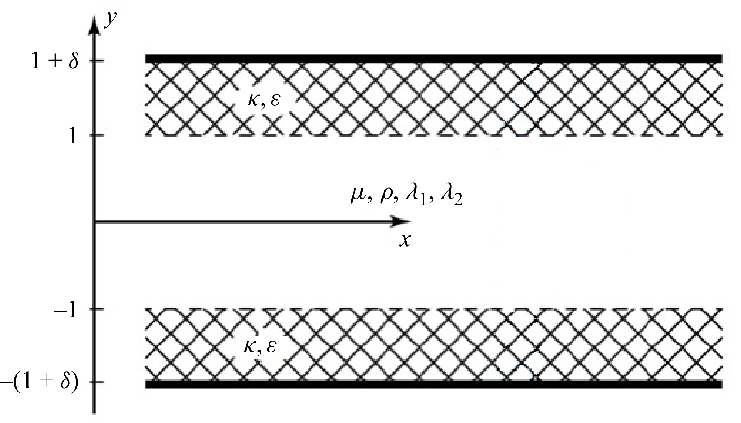


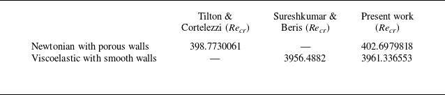

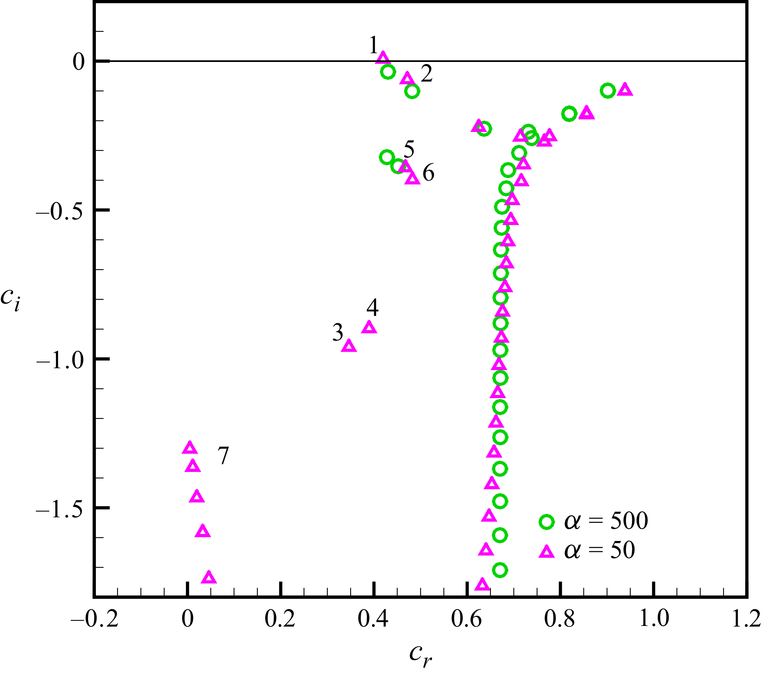


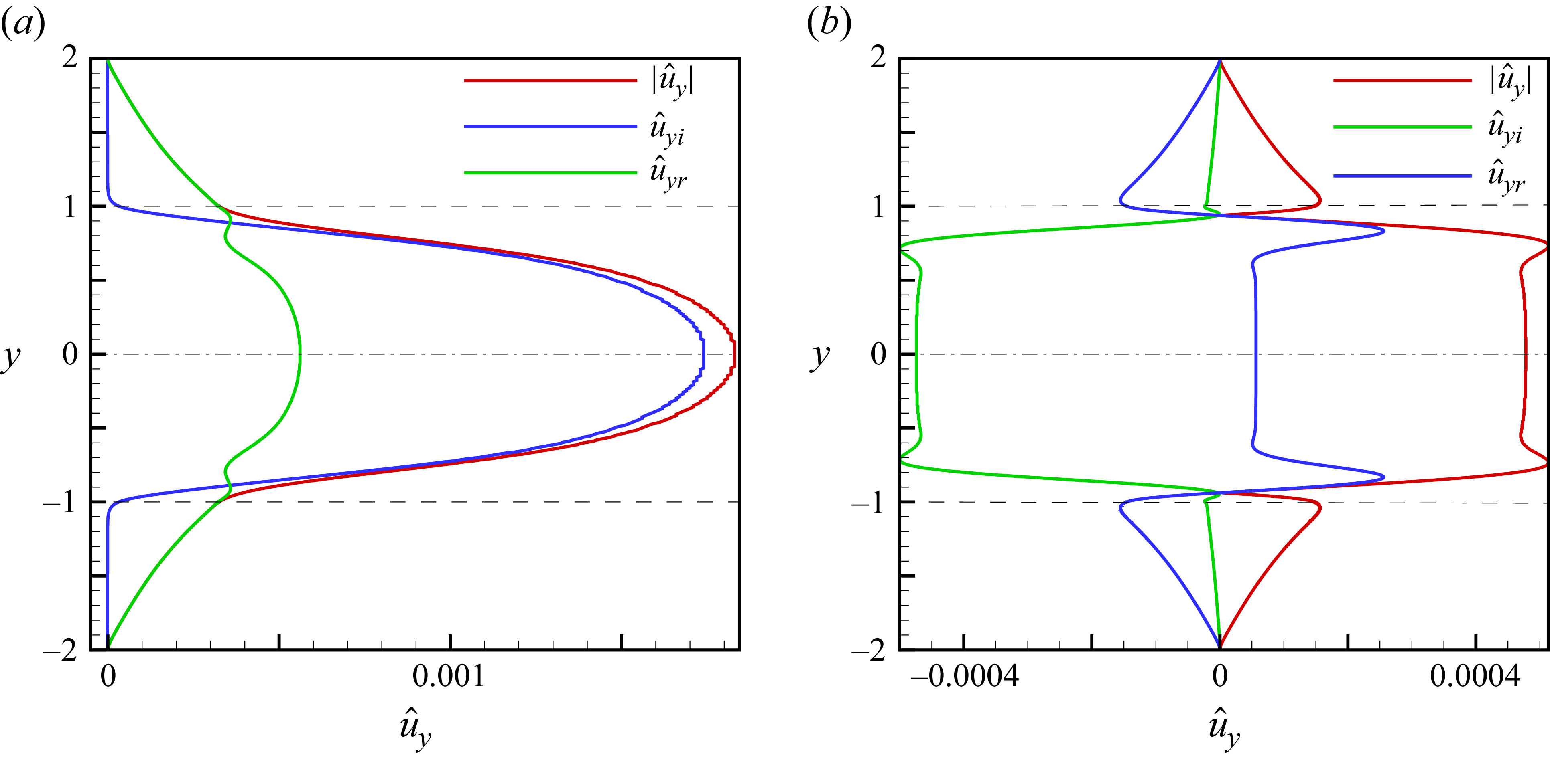


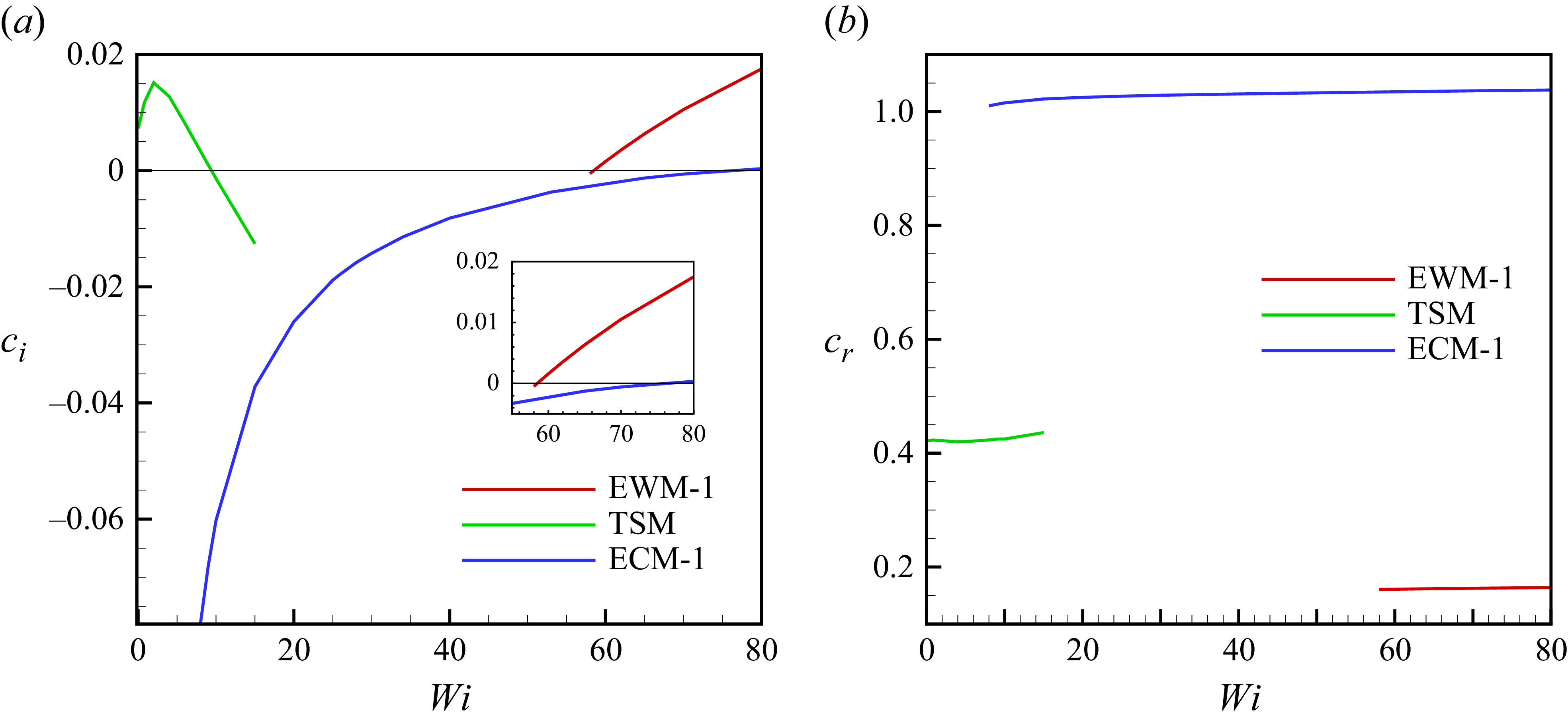


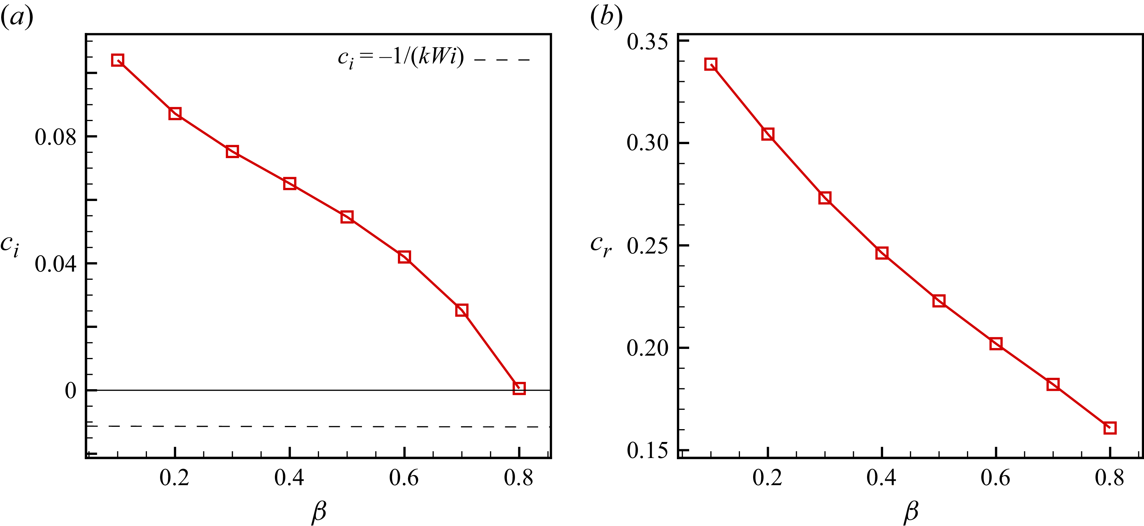


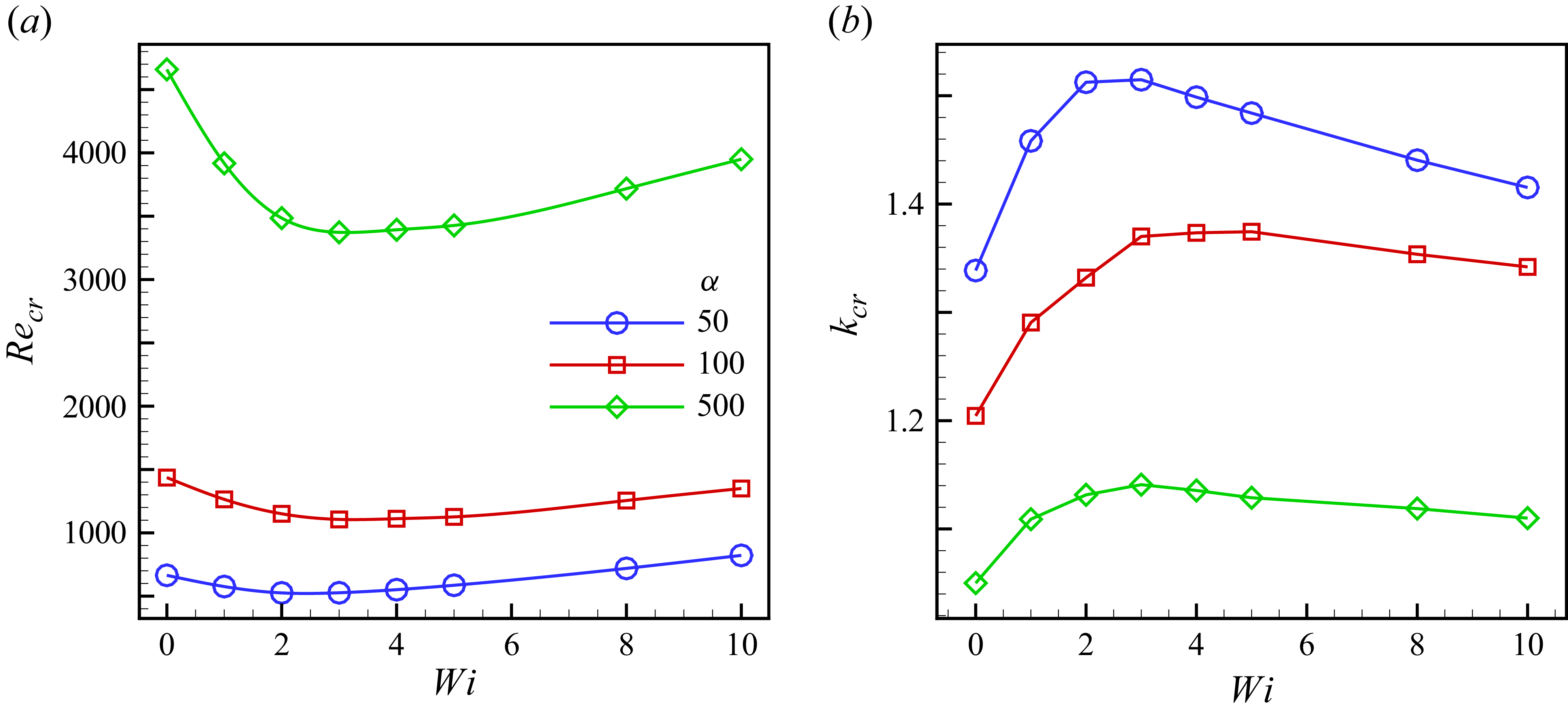


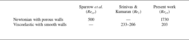


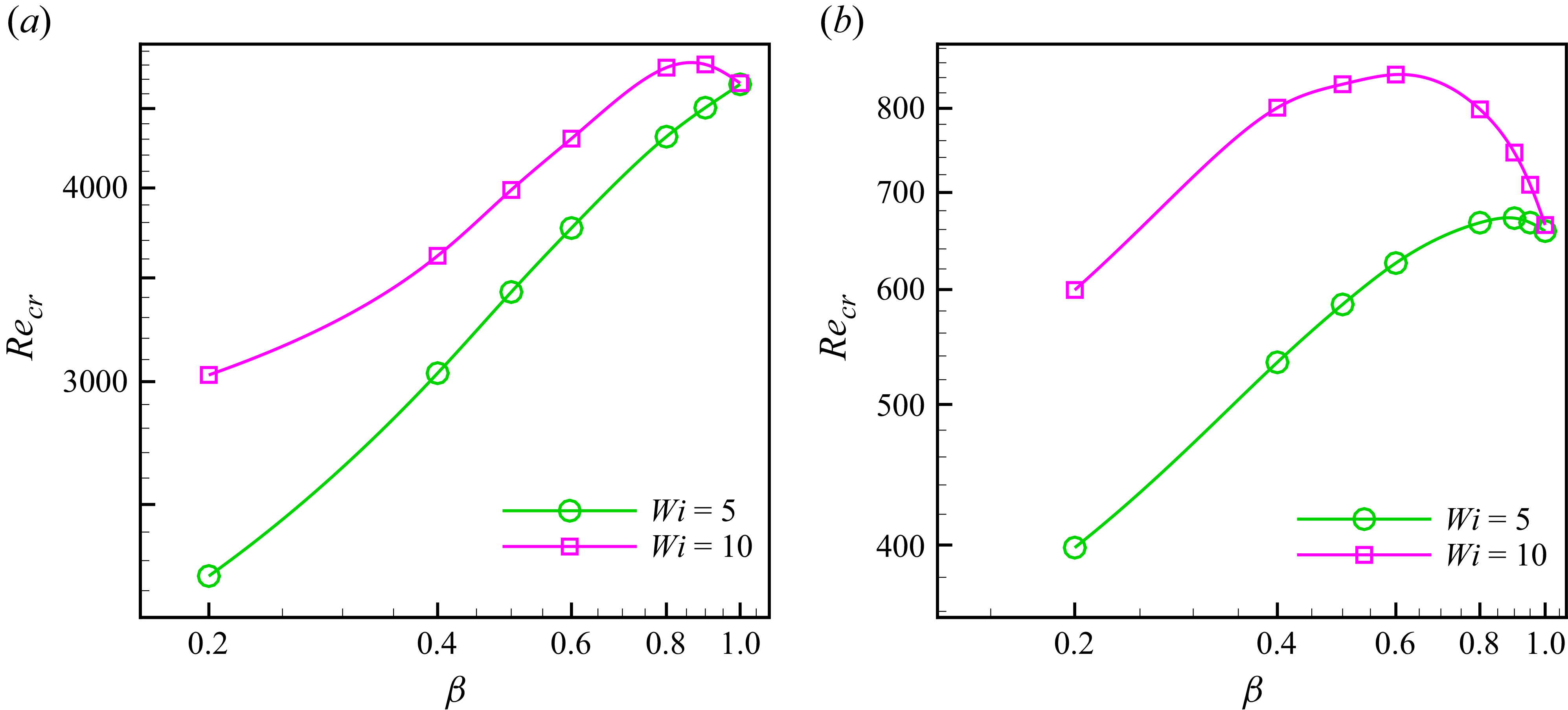


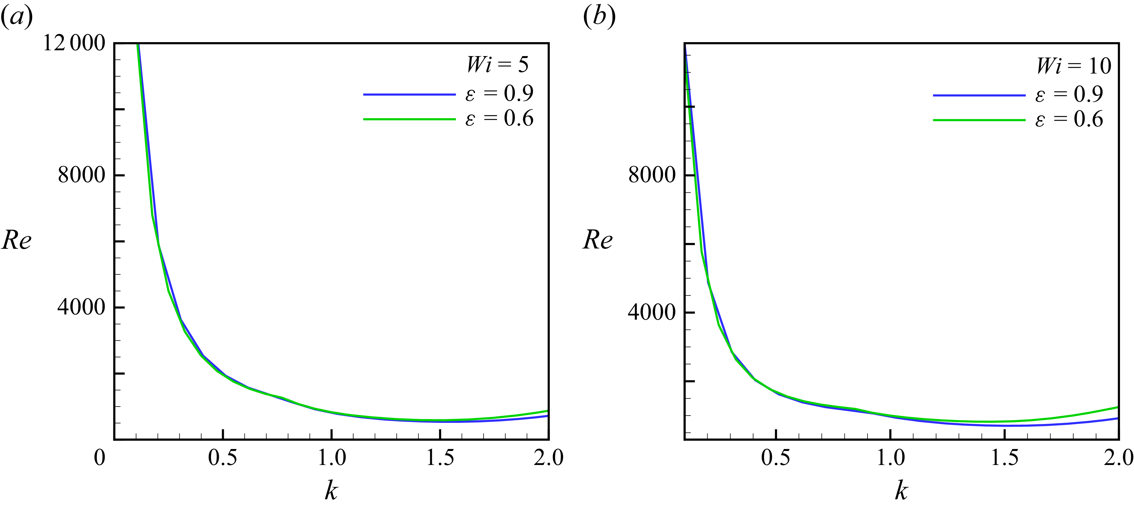


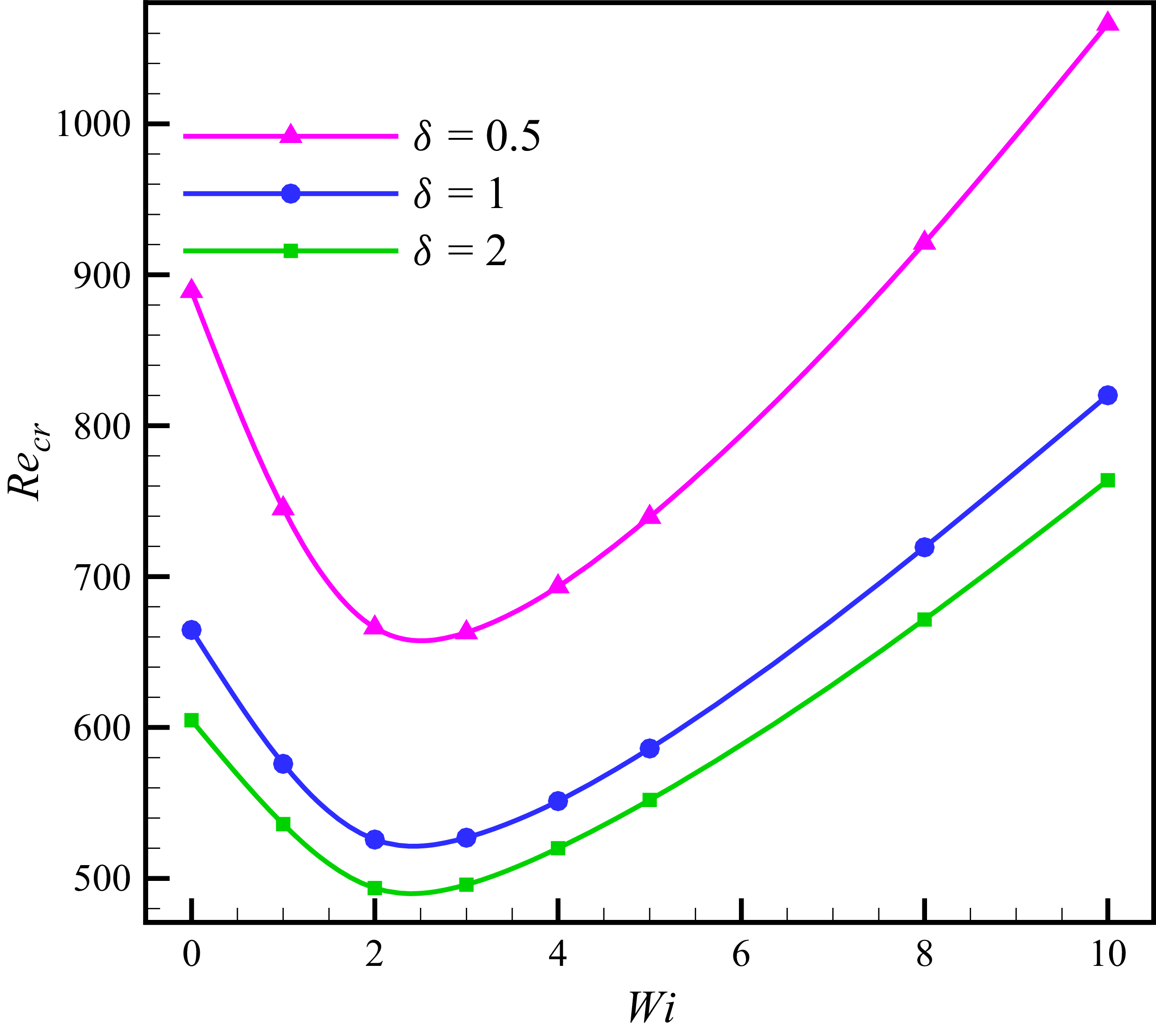


 Open access

