



1. Introduction
A branching process in a varying environment (BPVE) $(X_n)_{n\in \mathbb{N}}$
is defined as
$(X_n)_{n\in \mathbb{N}}$
is defined as
 \begin{equation} X_0 = 1, \qquad X_n = \sum_{j=1}^{X_{n-1}} \xi_{n,j}, \quad n\in\mathbb{N} = \{ 1, 2, \ldots \},\end{equation}
where $\{\xi_{n,j} \colon n,j\in\mathbb{N} \}$
are nonnegative integer-valued independent random variables such that, for each n, the variables
$\{\xi_{n,j} \colon n,j\in\mathbb{N} \}$
are nonnegative integer-valued independent random variables such that, for each n, the variables $\{ \xi_{n,j} \colon j\in\mathbb{N} \}$
are identically distributed; let
$\{ \xi_{n,j} \colon j\in\mathbb{N} \}$
are identically distributed; let $\xi_n$
denote a generic copy. Adding immigration leads to a branching process in a varying environment with immigration (BPVEI)
$\xi_n$
denote a generic copy. Adding immigration leads to a branching process in a varying environment with immigration (BPVEI) $(Y_n)_{n\in \mathbb{N}}$
, defined as
$(Y_n)_{n\in \mathbb{N}}$
, defined as
 \begin{equation} Y_0=0, \qquad Y_n=\sum_{j=1}^{Y_{n-1}}\xi_{n,j}+\varepsilon_n, \quad n\in\mathbb{N},\end{equation}
where $\{\xi_{n,j}, \varepsilon_n \colon n,j\in\mathbb{N} \}$
are nonnegative integer-valued independent random variables such that, for each n, the variables
$\{\xi_{n,j}, \varepsilon_n \colon n,j\in\mathbb{N} \}$
are nonnegative integer-valued independent random variables such that, for each n, the variables $\{\xi_{n,j} \colon j\in\mathbb{N}\}$
are identically distributed, and
$\{\xi_{n,j} \colon j\in\mathbb{N}\}$
are identically distributed, and $\xi_n$
is a generic copy.
$\xi_n$
is a generic copy.
Put $\overline{f}_n = \mathbb{E} (\xi_n)$
for the offspring mean in generation n. To exclude trivialities, we always assume that
$\overline{f}_n = \mathbb{E} (\xi_n)$
for the offspring mean in generation n. To exclude trivialities, we always assume that $\overline{f}_n \gt 0$
for all n. Let
$\overline{f}_n \gt 0$
for all n. Let $f_n(s) = \mathbb{E} (s^{\xi_n})$
,
$f_n(s) = \mathbb{E} (s^{\xi_n})$
, $s\in[0,1]$
, denote the generating function (g.f.) of the offspring distribution in the nth generation. As in [Reference Kevei and Kubatovics21], we are interested in branching processes in a nearly degenerate environment; that is, we always assume the following conditions:
$s\in[0,1]$
, denote the generating function (g.f.) of the offspring distribution in the nth generation. As in [Reference Kevei and Kubatovics21], we are interested in branching processes in a nearly degenerate environment; that is, we always assume the following conditions:
-
(C1) $\lim_{n\to\infty}\overline{f}_n = 1$
,
$\sum_{n=1}^{\infty}(1-\overline{f}_n)_+ = \infty$
, and
$\sum_{n=1}^\infty (\overline{f}_n - 1)_+ \lt \infty$
;
$\lim_{n\to\infty}\overline{f}_n = 1$
,
$\sum_{n=1}^{\infty}(1-\overline{f}_n)_+ = \infty$
, and
$\sum_{n=1}^\infty (\overline{f}_n - 1)_+ \lt \infty$
; -
(C2)
$\lim_{n\to\infty, \overline{f}_n \lt 1} {f_n''(1)}/({1-\overline{f}_n}) = \nu \in [0,\infty)$
, and the sequence
$\big({f_n''(1)}/{|1- \overline{f}_n|}\big)_{n}$
is bounded; -
(C3) if
$\nu\gt0$
, then
$\lim_{n\to \infty, \overline{f}_n \lt 1}{f_n'''(1)}/({1- \overline{f}_n}) = 0$
, and the sequence
$\big({f_n'''(1)}/{|1- \overline{f}_n|}\big)_{n}$
is bounded.








Here and later, $\lim_{n\to\infty, \overline{f}_n \lt 1}$
means that the convergence holds along the subsequence
$\lim_{n\to\infty, \overline{f}_n \lt 1}$
means that the convergence holds along the subsequence $\{n\colon \overline{f}_n \lt1\}$
. We allow
$\{n\colon \overline{f}_n \lt1\}$
. We allow $\overline{f}_n = 1$
, in which case we use the convention
$\overline{f}_n = 1$
, in which case we use the convention $0/0 = 0$
. Since by (C1) subcritical regimes dominate in the process,
$0/0 = 0$
. Since by (C1) subcritical regimes dominate in the process, $\mathbb{E} (X_n) = \prod_{j=1}^n \overline{f}_j \;=\!:\; \overline{f}_{0,n} \to 0$
as
$\mathbb{E} (X_n) = \prod_{j=1}^n \overline{f}_j \;=\!:\; \overline{f}_{0,n} \to 0$
as $n\to\infty$
, and the process dies out almost surely. Condition (C2) implies that
$n\to\infty$
, and the process dies out almost surely. Condition (C2) implies that $f_n''(1) \to 0$
, thus
$f_n''(1) \to 0$
, thus $f_n(s) \to s$
, and the branching mechanism converges to the degenerate branching.
$f_n(s) \to s$
, and the branching mechanism converges to the degenerate branching.
The theory of non-homogeneous branching processes started in [Reference Church10, Reference Fearn14]. Recent results in [Reference Kersting18, Reference Kersting and Vatutin19] have renewed interest in BPVEs. In [Reference Kersting18], a necessary and sufficient condition was obtained for almost sure extinction of regular processes; see also [Reference Bhattacharya and Perlman5, Reference Dolgopyat, Hebbar, Koralov and Perlman12] for the continuous-time and multitype cases, and [Reference Cardona-Tobón and Palau8] for a probabilistic proof. Nearly degenerate BPVEIs were introduced in [Reference Györfi, Ispány, Pap and Varga16], where it was assumed that the offspring have a Bernoulli distribution. In this case, the resulting process is a non-homogeneous first-order integer-valued autoregressive process (INAR(1)). INAR processes are important in various fields of applied probability; see the survey in [Reference Weiß29]. The setting of [Reference Györfi, Ispány, Pap and Varga16] was extended in [Reference Kevei20], and the multitype case was studied in [Reference Györfi, Ispány, Kevei and Pap15].
In [Reference Kevei and Kubatovics21] we analyzed BPVEs and BPVEIs under conditions (C1)–(C3). We showed that both BPVE processes conditioned on non-extinction and BPVEI processes without normalization converge in distribution to a geometric or a compound Poisson random variable. The results in [Reference Kevei and Kubatovics21] concern only the asymptotics of the one-dimensional distributions. In this paper, we continue the investigation of the long-term behavior of nearly degenerate BPVEs and BPVEIs and prove functional limit theorems in the Skorokhod space of càdlàg functions.
To derive convergence, it is crucial to find a proper scaling for the process. Condition (C1) implies that, for all nearly degenerate BPVEs, there is a sequence $(A(n))_{n\in\mathbb{N}}$
of natural numbers increasing to infinity such that
$(A(n))_{n\in\mathbb{N}}$
of natural numbers increasing to infinity such that
 \begin{equation} \overline{f}_{0,A(n)} \sim n^{-1} \quad \text{as $n\to\infty$},\end{equation}
which turns out to be the proper scaling. In what follows, we are interested in the processes $(X_{A(nt)})_{t\gt0}$
and
$(X_{A(nt)})_{t\gt0}$
and $(Y_{A(nt)})_{t \gt 0}$
, and to simplify the notation, A(nt) is meant as
$(Y_{A(nt)})_{t \gt 0}$
, and to simplify the notation, A(nt) is meant as $A(\lfloor nt \rfloor)$
.
$A(\lfloor nt \rfloor)$
.
The simplest example is given by
 \begin{align*} \overline{f}_n = \begin{cases} 1 - {\alpha}/{n}, & n \geq \lfloor \alpha \rfloor + 1, \\ 1, & \text{otherwise} \end{cases}\end{align*}
for some $\alpha \gt 0$
. Then there exists
$\alpha \gt 0$
. Then there exists $c \gt 0$
such that
$c \gt 0$
such that $\overline{f}_{0,n} \sim c n^{-\alpha}$
as
$\overline{f}_{0,n} \sim c n^{-\alpha}$
as $n\to\infty$
. Thus, with
$n\to\infty$
. Thus, with $A(n) = \lfloor c^{1/\alpha} n^{1 / \alpha} \rfloor$
, (3) holds.
$A(n) = \lfloor c^{1/\alpha} n^{1 / \alpha} \rfloor$
, (3) holds.
In Section 2.1, for the conditioned process we prove that $\mathcal{L}((X_{A(nt)})_{t \gt 0} \mid X_{A(n)} \gt 0)$
, the law of
$\mathcal{L}((X_{A(nt)})_{t \gt 0} \mid X_{A(n)} \gt 0)$
, the law of $(X_{A(nt)})_{t \gt 0}$
conditioned on the event
$(X_{A(nt)})_{t \gt 0}$
conditioned on the event $\{ X_{A(n)} \gt 0 \}$
, converges in distribution in the Skorokhod space of càdlàg functions to a time-transformed simple birth-and-death process conditioned on survival. We analyze the limit process and explore its relation to the quasi-stationary distribution. In Section 2.2, for the immigration process we show that
$\{ X_{A(n)} \gt 0 \}$
, converges in distribution in the Skorokhod space of càdlàg functions to a time-transformed simple birth-and-death process conditioned on survival. We analyze the limit process and explore its relation to the quasi-stationary distribution. In Section 2.2, for the immigration process we show that $(Y_{A(nt)})_{t \gt 0}$
converges to a time-transformed continuous-time Markov branching process with immigration. In both cases, we only scale in time; therefore, the limit processes are continuous-time Markov chains with state spaces
$(Y_{A(nt)})_{t \gt 0}$
converges to a time-transformed continuous-time Markov branching process with immigration. In both cases, we only scale in time; therefore, the limit processes are continuous-time Markov chains with state spaces $\mathbb{N}$
and
$\mathbb{N}$
and $\mathbb{N} \cup \{ 0 \}$
, respectively. Convergence to the Poisson process is a well-studied area; see [Reference Billingsley6, Section 3.12]. However, we are not aware of results on convergence to non-monotone Markov chains. The proof of the convergence of the finite-dimensional distributions is standard, but the proof of tightness is rather troublesome. We also note that the limit processes in both cases are naturally defined on
$\mathbb{N} \cup \{ 0 \}$
, respectively. Convergence to the Poisson process is a well-studied area; see [Reference Billingsley6, Section 3.12]. However, we are not aware of results on convergence to non-monotone Markov chains. The proof of the convergence of the finite-dimensional distributions is standard, but the proof of tightness is rather troublesome. We also note that the limit processes in both cases are naturally defined on $(0,\infty)$
, which is not common for Markov processes. For the conditioned process
$(0,\infty)$
, which is not common for Markov processes. For the conditioned process $(X_n)$
, the limit is non-homogeneous even after a natural time transformation, and its existence can be obtained via the construction of an entrance law. For the immigration process
$(X_n)$
, the limit is non-homogeneous even after a natural time transformation, and its existence can be obtained via the construction of an entrance law. For the immigration process $(Y_n)$
, the limit is a time-transformed stationary process. Stationary processes, in discrete and continuous time, are commonly defined on
$(Y_n)$
, the limit is a time-transformed stationary process. Stationary processes, in discrete and continuous time, are commonly defined on $\mathbb{Z}$
or on
$\mathbb{Z}$
or on $(-\infty, \infty)$
, respectively; see, e.g., [Reference Barndorff-Nielsen, Benth and Veraart4, Reference Brockwell and Davis7].
$(-\infty, \infty)$
, respectively; see, e.g., [Reference Barndorff-Nielsen, Benth and Veraart4, Reference Brockwell and Davis7].
Section 2 contains the main results, while proofs and auxiliary results are gathered in Section 3.
2. Main results
2.1. Nearly degenerate BPVEs
Consider a simple continuous-time birth-and-death process $(Z(u))_{u\geq -w}$
defined on the time interval
$(Z(u))_{u\geq -w}$
defined on the time interval $u \in [-w, \infty)$
for some
$u \in [-w, \infty)$
for some $w \geq 0$
, with birth rate
$w \geq 0$
, with birth rate ${\nu}/{2}$
and death rate
${\nu}/{2}$
and death rate $1 + {\nu}/{2}$
. That is, in state n, the birth and death rates are
$1 + {\nu}/{2}$
. That is, in state n, the birth and death rates are $n{\nu}/{2}$
and
$n{\nu}/{2}$
and $n (1 + {\nu}/{2})$
, respectively. Note that this is a usual birth-and-death process with a shifted time domain. The transition-generating function of Z is given (see, e.g., [Reference Athreya and Ney3, III.5], [Reference Allen1, 6.4.3]) as
$n (1 + {\nu}/{2})$
, respectively. Note that this is a usual birth-and-death process with a shifted time domain. The transition-generating function of Z is given (see, e.g., [Reference Athreya and Ney3, III.5], [Reference Allen1, 6.4.3]) as
 \begin{align} F(s,t) = \mathbb{E}\big[s^{Z(t + u)} \mid Z(u) = 1\big] & = \frac{(1 + {\nu}/{2})(s-1) - {\mathrm{e}}^{t}(s{\nu}/{2} - (1 + {\nu}/{2}))} {{\nu}(s-1)/2 - {\mathrm{e}}^{t}(s{\nu}/{2} - (1 + {\nu}/{2}))} \nonumber \\ & = 1 - {\mathrm{e}}^{-t}\bigg(\frac{1}{1-s} + \frac{\nu}{2}(1 - {\mathrm{e}}^{-t})\bigg)^{-1}, \end{align}
where $s \in [0,1]$
,
$s \in [0,1]$
, $u \geq -w$
, and
$u \geq -w$
, and $t \geq 0$
.
$t \geq 0$
.
Let $a, b \in\mathbb{R}$
with
$a, b \in\mathbb{R}$
with $a\lt b$
. The Skorokhod spaces of real-valued càdlàg functions on [a, b] and
$a\lt b$
. The Skorokhod spaces of real-valued càdlàg functions on [a, b] and $[a,\infty)$
with the usual metric are denoted by D([a, b]) and
$[a,\infty)$
with the usual metric are denoted by D([a, b]) and $D([a,\infty))$
respectively, and
$D([a,\infty))$
respectively, and $\stackrel{\mathcal{D}}{\longrightarrow}$
represents convergence in distribution in the Skorokhod space. A random variable Y has a geometric distribution with parameter
$\stackrel{\mathcal{D}}{\longrightarrow}$
represents convergence in distribution in the Skorokhod space. A random variable Y has a geometric distribution with parameter $p \in (0,1]$
, written
$p \in (0,1]$
, written $Y \sim \operatorname{Geom}(p)$
, if
$Y \sim \operatorname{Geom}(p)$
, if $\mathbb{P} ( Y = k) = (1- p)^{k-1} p$
for
$\mathbb{P} ( Y = k) = (1- p)^{k-1} p$
for $k = 1, 2, \ldots$
Theorem 1. Let $(X_n)_{n\in\mathbb{N}}$
be a BPVE satisfying conditions (C1)–(C3). Then, for any
$(X_n)_{n\in\mathbb{N}}$
be a BPVE satisfying conditions (C1)–(C3). Then, for any $\varepsilon \in (0,1]$
,
$\varepsilon \in (0,1]$
,
 \begin{align*} \mathcal{L}\big((X_{A(nt)})_{t\geq\varepsilon} \mid X_{A(n)} \gt 0\big) \stackrel{\mathcal{D}}{\longrightarrow} \mathcal{L}\big(({Z}(\log t))_{t\geq\varepsilon} \mid Z(0) \gt 0\big) \end{align*}
as $n \to \infty$
, where
$n \to \infty$
, where $(Z(u))_{u\geq\log\varepsilon}$
is a simple birth-and-death process with the initial distribution
$(Z(u))_{u\geq\log\varepsilon}$
is a simple birth-and-death process with the initial distribution $Z(\log\varepsilon) \sim \operatorname{Geom}({2}/({2+\nu}))$
, birth rate
$Z(\log\varepsilon) \sim \operatorname{Geom}({2}/({2+\nu}))$
, birth rate ${\nu}/{2}$
, and death rate
${\nu}/{2}$
, and death rate $1 + {\nu}/{2}$
.
$1 + {\nu}/{2}$
.
Note that if $\nu = 0$
, Z(u) is a simple death process with death rate 1 and the initial distribution
$\nu = 0$
, Z(u) is a simple death process with death rate 1 and the initial distribution $Z( \log \varepsilon ) = 1$
.
$Z( \log \varepsilon ) = 1$
.
Since the limit process $(Z(\log t))_{t \geq \varepsilon}$
is conditioned on non-extinction at
$(Z(\log t))_{t \geq \varepsilon}$
is conditioned on non-extinction at $t=1$
, it is no surprise that the limit behaves differently for
$t=1$
, it is no surprise that the limit behaves differently for $t\in[\varepsilon, 1)$
and
$t\in[\varepsilon, 1)$
and $t\geq 1$
. In fact, for
$t\geq 1$
. In fact, for $t\geq 1$
, the limit reduces to
$t\geq 1$
, the limit reduces to $(Z(\log t))_{t\geq 1}$
with initial distribution
$(Z(\log t))_{t\geq 1}$
with initial distribution $\operatorname{Geom}({2}/({2 + \nu}))$
.
$\operatorname{Geom}({2}/({2 + \nu}))$
.
Note that Theorem 1 holds for any $\varepsilon \gt 0$
; however, we cannot take
$\varepsilon \gt 0$
; however, we cannot take $\varepsilon = 0$
because the limit process is not defined on (0,1]. That is, Z is not defined on
$\varepsilon = 0$
because the limit process is not defined on (0,1]. That is, Z is not defined on $(-\infty, \infty)$
. To see the behavior on (0, 1], we first show that the limit process can be extended to (0,1]. To do that, we need some properties of the limit process.
$(-\infty, \infty)$
. To see the behavior on (0, 1], we first show that the limit process can be extended to (0,1]. To do that, we need some properties of the limit process.
For $a \in [0,1]$
,
$a \in [0,1]$
, $\nu \geq 0$
, we introduce the notation
$\nu \geq 0$
, we introduce the notation
 \begin{equation*} h_a(s) = 1 - a\bigg(\frac{1}{1-s} + \frac{\nu}{2}(1-a)\bigg)^{-1},\end{equation*}
that is, $h_a$
is the generating function of a linear fractional distribution with mean a. Linear fractional distributions are an important class of offspring distributions because of the possible explicit calculations; see [Reference Athreya and Ney3, Chapter I.4], with
$h_a$
is the generating function of a linear fractional distribution with mean a. Linear fractional distributions are an important class of offspring distributions because of the possible explicit calculations; see [Reference Athreya and Ney3, Chapter I.4], with
 $$p = \frac{\nu (1-a)}{2 + \nu (1-a)}, \qquad b = \frac{4 a}{(2 + \nu (1-a))^2}.$$
We stress that $h_a$
depends on both a and
$h_a$
depends on both a and $\nu$
; however, since the latter parameter is fixed in our setup, it is suppressed in our notation. Note that we also allow the degenerate case
$\nu$
; however, since the latter parameter is fixed in our setup, it is suppressed in our notation. Note that we also allow the degenerate case $\nu=0$
, when
$\nu=0$
, when $h_a(s)$
is the g.f. of a Bernoulli-distributed variable with parameter a. Recall the important property of linear fractional distributions that
$h_a(s)$
is the g.f. of a Bernoulli-distributed variable with parameter a. Recall the important property of linear fractional distributions that $h_a ( h_b(s)) = h_{ab}(s)$
for all
$h_a ( h_b(s)) = h_{ab}(s)$
for all $a,b \in [0,1]$
. With this notation, the function F defined in (4) can be expressed as
$a,b \in [0,1]$
. With this notation, the function F defined in (4) can be expressed as $F(s,t) = h_{{\mathrm{e}}^{-t}}(s)$
.
$F(s,t) = h_{{\mathrm{e}}^{-t}}(s)$
.
Let us define the time-changed process
 \begin{equation} U(t) = Z(\log t), \quad t \geq \varepsilon.\end{equation}
Then, for $\varepsilon \leq u \lt t$
and
$\varepsilon \leq u \lt t$
and $x_0 \in \{1, 2, \ldots \}$
,
$x_0 \in \{1, 2, \ldots \}$
,
 \begin{align} \mathbb{E} \big[s^{{U}(t)} \mid {U}(u) = x_0\big] & = \mathbb{E}\big[s^{Z(\log t)} \mid Z(\log u) = x_0\big] \nonumber \\[5pt] & = \big(\mathbb{E}\big[s^{Z(\log t)} \mid Z(\log u) = 1\big]\big)^{x_0} \nonumber \\[5pt] & = \big(h_{{\mathrm{e}}^{-(\log t - \log u)}}(s)\big)^{x_0} = (h_{u/t}(s))^{x_0}. \end{align}
We analyze the limit process defined in (5). Put $p = {2}/({2+\nu})$
,
$p = {2}/({2+\nu})$
, $q = 1-p$
. Define the generating function for
$q = 1-p$
. Define the generating function for $t \in (0,1]$
as
$t \in (0,1]$
as
 \begin{equation*} g_t(s)= \frac{ps}{1-qs} \,\frac{t^{-1} (1 - h_{t}(0) )}{1 - h_{t}(0) q s}= \sum_{x=1}^\infty p q^{x-1} t^{-1} ( 1 - h_{t}(0)^x) s^x.\end{equation*}
Note that $t^{-1} (1 - h_{t}(0)) = {p}/({1 - q t})\to p$
as
$t^{-1} (1 - h_{t}(0)) = {p}/({1 - q t})\to p$
as $t \downarrow 0$
. Furthermore,
$t \downarrow 0$
. Furthermore, $g_t$
is the generating function of
$g_t$
is the generating function of $V + W_t$
, where
$V + W_t$
, where $V \sim \operatorname{Geom}(p)$
,
$V \sim \operatorname{Geom}(p)$
, $W_t + 1 \sim \operatorname{Geom}({p}/({1 - q t}))$
, and V and
$W_t + 1 \sim \operatorname{Geom}({p}/({1 - q t}))$
, and V and $W_t$
are independent. Let
$W_t$
are independent. Let $\mathbb{P}_\varepsilon$
denote the law of the process
$\mathbb{P}_\varepsilon$
denote the law of the process $(U(t)_{t \in [\varepsilon, 1]})$
under the initial distribution
$(U(t)_{t \in [\varepsilon, 1]})$
under the initial distribution $U(\varepsilon) \sim \operatorname{Geom}(p)$
.
$U(\varepsilon) \sim \operatorname{Geom}(p)$
.
The distribution $\operatorname{Geom}(p)$
is the extremal quasi-stationary distribution of the birth-and-death process Z; see [Reference Collet, Martnez and San Martn11, p. 106]. This means that
$\operatorname{Geom}(p)$
is the extremal quasi-stationary distribution of the birth-and-death process Z; see [Reference Collet, Martnez and San Martn11, p. 106]. This means that
 \begin{align*}\mathbb{E}_\varepsilon \big[ s^{U(1)} \mid U(1) \gt 0\big] = \frac{ps}{1-qs}= \mathbb{E}_\varepsilon \big(s^{U(\varepsilon)}\big),\end{align*}
i.e., conditioned on non-extinction, the distribution of U(1) is the same as the initial distribution. The second statement below is an extension of the quasi-stationary property, which corresponds to $t = 1$
.
$t = 1$
.
The limit process as $\varepsilon \downarrow 0$
is defined on (0,1] (or on
$\varepsilon \downarrow 0$
is defined on (0,1] (or on $(0,\infty)$
), which means that there is no initial distribution for the Markov process. The existence of the process in this case can be handled via entrance laws. That is, if we start the process at time
$(0,\infty)$
), which means that there is no initial distribution for the Markov process. The existence of the process in this case can be handled via entrance laws. That is, if we start the process at time $\varepsilon \gt 0$
with the initial law given by
$\varepsilon \gt 0$
with the initial law given by $g_\varepsilon$
and run it up to time
$g_\varepsilon$
and run it up to time $t \gt \varepsilon$
according to the non-homogeneous transition probabilities given by
$t \gt \varepsilon$
according to the non-homogeneous transition probabilities given by $k_{\varepsilon, t; x_0}$
, then the process at time t has the distribution given by
$k_{\varepsilon, t; x_0}$
, then the process at time t has the distribution given by $g_{t}$
.
$g_{t}$
.
Lemma 1. Fix $\varepsilon \in (0,1)$
arbitrarily. Then, for
$\varepsilon \in (0,1)$
arbitrarily. Then, for $\varepsilon \leq u \lt t \leq 1$
and
$\varepsilon \leq u \lt t \leq 1$
and $x_0 \in \mathbb{N}$
, the generating function of the conditional transition probabilities is given by
$x_0 \in \mathbb{N}$
, the generating function of the conditional transition probabilities is given by
 \begin{equation} \mathbb{E}\big[s^{U(t)} \mid U(u) = x_0, U(1) \gt 0 \big] = \frac{(h_{u/t}(s))^{x_0} - (h_{u/t}(h_{t}(0)s))^{x_0}}{1 - (h_{u}(0))^{x_0}} \;=\!:\; k_{u,t;x_0}(s). \end{equation}
The family of laws with generating functions $(g_t)_{t \in (0,1]}$
is an entrance law for the transition-generating functions
$(g_t)_{t \in (0,1]}$
is an entrance law for the transition-generating functions $k_{u,t;x}$
; that is, for
$k_{u,t;x}$
; that is, for $\varepsilon \in (0,1]$
and for any
$\varepsilon \in (0,1]$
and for any $t \in [\varepsilon, 1]$
,
$t \in [\varepsilon, 1]$
,
 \begin{align*} \mathbb{E}_\varepsilon\big[s^{U(t)} \mid U(1) \gt 0 \big] = g_t(s). \end{align*}
Entrance laws for homogeneous Markov chains were treated in [Reference Chung9, Definition I.1.1], [Reference Rogers and Williams26, III.5.39], and [Reference Sharpe28, Chapters I.1 and V]. In [Reference Rogers and Williams26], the existence of a càdlàg Markov process on $(0,\infty)$
with the given transition probabilities and entrance laws was proved. In the general non-homogeneous setup, the problem was already investigated in 1936 in [Reference Kolmogoroff22] (for the English translation see [Reference Kolmogorov23]), where entrance laws are called absolute probabilities. In our setup, the transition probabilities are non-homogeneous even after the time transformation to
$(0,\infty)$
with the given transition probabilities and entrance laws was proved. In the general non-homogeneous setup, the problem was already investigated in 1936 in [Reference Kolmogoroff22] (for the English translation see [Reference Kolmogorov23]), where entrance laws are called absolute probabilities. In our setup, the transition probabilities are non-homogeneous even after the time transformation to $(-\infty,0]$
due to the conditioning at 0.
$(-\infty,0]$
due to the conditioning at 0.
The existence of an entrance law, together with Kolmogorov’s consistency theorem, implies that there exists a Markov process $\widetilde U$
on (0, 1] with the given marginals and transition probabilities. For any
$\widetilde U$
on (0, 1] with the given marginals and transition probabilities. For any $\varepsilon \gt 0$
, the process
$\varepsilon \gt 0$
, the process $\widetilde U$
on
$\widetilde U$
on $[\varepsilon, 1]$
is a time-transformed birth-and-death process conditioned on non-extinction; thus, it has a càdlàg version. To show the existence of a càdlàg version on the whole of (0, 1], we have to demonstrate that we can glue the process together backwards in time in a consistent way. This can be done using time reversal, as the reversed process is also Markov, which can be continued forward in time; see the proof for the details.
$[\varepsilon, 1]$
is a time-transformed birth-and-death process conditioned on non-extinction; thus, it has a càdlàg version. To show the existence of a càdlàg version on the whole of (0, 1], we have to demonstrate that we can glue the process together backwards in time in a consistent way. This can be done using time reversal, as the reversed process is also Markov, which can be continued forward in time; see the proof for the details.
Corollary 1. There exists a càdlàg Markov process $(\widetilde U(t))_{t \in (0,1]}$
such that its transition probabilities are given by the generating functions
$(\widetilde U(t))_{t \in (0,1]}$
such that its transition probabilities are given by the generating functions $ k_{u,t;x}(s) = \mathbb{E}[s^{\widetilde U(t)} \mid \widetilde U(u) = x]$
, and
$ k_{u,t;x}(s) = \mathbb{E}[s^{\widetilde U(t)} \mid \widetilde U(u) = x]$
, and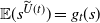 $\mathbb{E}(s^{\widetilde U(t)}) = g_t(s)$
for each
$\mathbb{E}(s^{\widetilde U(t)}) = g_t(s)$
for each $t \in (0,1]$
.
$t \in (0,1]$
.
As we noted earlier,
 $$\lim_{t \downarrow 0} g_t(s) = \frac{ps}{1-qs} \frac{p}{1-qs},$$
that is,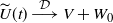 $\widetilde U(t) \stackrel{\mathcal{D}}{\longrightarrow} V + W_0$
as
$\widetilde U(t) \stackrel{\mathcal{D}}{\longrightarrow} V + W_0$
as $t \downarrow 0$
where
$t \downarrow 0$
where $V, W_0$
are independent,
$V, W_0$
are independent, $V, W_0 + 1 \sim \operatorname{Geom}(p)$
. However, contrary to the homogeneous case, see [Reference Rogers and Williams26, III.39],
$V, W_0 + 1 \sim \operatorname{Geom}(p)$
. However, contrary to the homogeneous case, see [Reference Rogers and Williams26, III.39], $\widetilde U(t)$
as
$\widetilde U(t)$
as $t \downarrow 0$
does not converge in probability. Indeed, a short calculation shows that, for
$t \downarrow 0$
does not converge in probability. Indeed, a short calculation shows that, for $\alpha \in (0,1)$
, as
$\alpha \in (0,1)$
, as $t \downarrow 0$
,
$t \downarrow 0$
,
 \begin{align*} k_{\alpha t, t; x_0}(s) = \frac{(h_\alpha(s))^{x_0} - (h_\alpha(h_t(0)s))^{x_0}}{1 - (h_{\alpha t}(0))^{x_0}} \longrightarrow \frac{s}{\alpha} (h_{\alpha}(s))^{x_0 -1} h_{\alpha}'(s), \quad s \in [0,1],\end{align*}
that is, the transition probabilities around 0 converge to a nontrivial distribution.
As a consequence of the existence result above and Theorem 1, we can extend the convergence to (0, 1]. The theory of Skorokhod spaces of càdlàg functions on noncompact domains other than $[0,\infty)$
is not well established. In [Reference Whitt30, Section 12.9], convergence on D(I) with I being an interval of
$[0,\infty)$
is not well established. In [Reference Whitt30, Section 12.9], convergence on D(I) with I being an interval of $\mathbb{R}$
is defined as the convergence on all compact subintervals [a, b] of I, where both a and b are either continuity points of the limit or boundary points of I. However, the results in [Reference Whitt30] are only spelled out for
$\mathbb{R}$
is defined as the convergence on all compact subintervals [a, b] of I, where both a and b are either continuity points of the limit or boundary points of I. However, the results in [Reference Whitt30] are only spelled out for $I = [0,\infty)$
and for the strong
$I = [0,\infty)$
and for the strong $M_1$
topology. In [Reference Iksanov, Marynych and Meiners17, Section 2.2], the authors consider convergence in
$M_1$
topology. In [Reference Iksanov, Marynych and Meiners17, Section 2.2], the authors consider convergence in $D(\mathbb{R})$
. Therefore, instead of claiming convergence on (0, 1], with a simple transformation we prove convergence in the more common function space
$D(\mathbb{R})$
. Therefore, instead of claiming convergence on (0, 1], with a simple transformation we prove convergence in the more common function space $D([1,\infty))$
.
$D([1,\infty))$
.
Corollary 2. Under the assumptions of Theorem 1,
 \begin{align*} \mathcal{L}((X_{A({n}/{t})-})_{t \geq 1} \mid X_{A(n)} \gt 0) \stackrel{\mathcal{D}}{\longrightarrow} \mathcal{L}((\widetilde U(({1}/{t})-))_{t \geq 1}) \quad \text{as $n\to\infty$}. \end{align*}
2.2. Nearly degenerate BPVEIs
Consider a BPVEI $(Y_n)_{n\in\mathbb{N}}$
as defined in (2), and introduce the notation
$(Y_n)_{n\in\mathbb{N}}$
as defined in (2), and introduce the notation
 \begin{align*}m_{n,k} \;:\!=\; \mathbb{E}[\varepsilon_n (\varepsilon_n - 1) \cdots (\varepsilon_n - k +1)], \quad k\in \mathbb{N},\end{align*}
for the factorial moments of the immigration in generation n. In what follows, we suppose that $(Y_n)_{n\in\mathbb{N}}$
is a nearly degenerate BPVEI; that is, its offspring distribution satisfies (C1)–(C3). We further assume that one of the following conditions holds:
$(Y_n)_{n\in\mathbb{N}}$
is a nearly degenerate BPVEI; that is, its offspring distribution satisfies (C1)–(C3). We further assume that one of the following conditions holds:
-
(C4)
$\lim_{n\to\infty, \overline{f}_n \lt 1}{m_{n,k}}/({k!(1-\overline{f}_n)}) = \lambda_k$
,
$k = 1,2,\ldots, K$
, for some
$K \geq 2$
, such that
$\lambda_K=0$
and the sequences
$({m_{n,k}}/({k!|1-\overline{f}_n|}))_{n}$
are bounded for each
$k\leq K$
; -
(C4′)
$\lim_{n\to\infty, \overline{f}_n \lt 1}{m_{n,k}}/({k!(1-\overline{f}_n)}) = \lambda_k$
,
$k = 1,2,\ldots$
, such that
$\limsup_{n\to\infty}\lambda_n^{1/n} \leq 1$
and the sequences
$({m_{n,k}}/({k!|1-\overline{f}_n|}))_{n}$
are bounded for all k.










For BPVEIs, the limit processes are continuous-time Markov branching processes with immigration, defined as follows. Each individual has an exponentially distributed lifetime with parameter $\alpha$
, and upon death it leaves a random number of offspring
$\alpha$
, and upon death it leaves a random number of offspring $\xi$
. Furthermore, a random number of immigrants
$\xi$
. Furthermore, a random number of immigrants $\varepsilon$
arrive at random times determined by a Poisson process of intensity
$\varepsilon$
arrive at random times determined by a Poisson process of intensity $\beta$
. All the quantities involved are independent. The offspring- and immigration-generating functions are
$\beta$
. All the quantities involved are independent. The offspring- and immigration-generating functions are $f(s) = \sum_{k=0}^\infty \mathbb{P}(\xi = k) s^k$
and
$f(s) = \sum_{k=0}^\infty \mathbb{P}(\xi = k) s^k$
and $h(s) = \sum_{k=1}^\infty \mathbb{P} (\varepsilon = k) s^k$
,
$h(s) = \sum_{k=1}^\infty \mathbb{P} (\varepsilon = k) s^k$
, $|s|\leq 1$
, where we may and do assume that
$|s|\leq 1$
, where we may and do assume that $\mathbb{P} (\xi = 1) = 0$
and
$\mathbb{P} (\xi = 1) = 0$
and $\mathbb{P}(\varepsilon = 0) = 0$
.
$\mathbb{P}(\varepsilon = 0) = 0$
.
When there is no immigration, we obtain the well-known class of continuous-time Markov branching processes; see [Reference Athreya and Ney3, Chapter III]. In particular, a birth-and-death process is a special continuous-time branching process with $\alpha = 1 + \nu$
and
$\alpha = 1 + \nu$
and
 \begin{align*} f(s) = \frac{1}{1 + \nu}\bigg( 1 + \frac{\nu}{2} + \frac{\nu}{2} s^2 \bigg).\end{align*}
Continuous-time Markov branching processes with immigration are less studied, though they were introduced in [Reference Sevast’yanov27] in 1957. Simple birth-and-death processes with immigration are discussed in detail in [Reference Allen1, Section 6.4.4], where immigrants arrive one by one. For some recent references, see [Reference Li, Chen and Pakes24, Reference Li and Li25].
Let $(W(t))_{t\geq - w}$
denote the resulting continuous-time branching process with immigration on the time interval
$(W(t))_{t\geq - w}$
denote the resulting continuous-time branching process with immigration on the time interval $t \in [\!-w, \infty)$
,
$t \in [\!-w, \infty)$
, $w \geq 0$
, and introduce the notation
$w \geq 0$
, and introduce the notation $G(s,t) = \mathbb{E}(s^{W(t+u)} \mid$ $W(u) =0)$
,
$W(u) =0)$
, $t \geq 0$
,
$t \geq 0$
, $u \geq -w$
,
$u \geq -w$
, $s \in [0,1]$
. Then G(s, t) satisfies the Kolmogorov forward equation (see [Reference Li, Chen and Pakes24, (2.5)])
$s \in [0,1]$
. Then G(s, t) satisfies the Kolmogorov forward equation (see [Reference Li, Chen and Pakes24, (2.5)])
 \begin{equation*} \frac{\partial}{\partial t} G(s,t) = a(s) \frac{\partial}{\partial s} G(s,t) + b(s) G(s,t)\end{equation*}
with boundary condition $G(s,0) = 1$
, where
$G(s,0) = 1$
, where
 \begin{equation}a(s) = \alpha(f(s) - s), \qquad b(s) = \beta(h(s) - 1).\end{equation}
Theorem 2. Assume that the BPVEI $(Y_n)_{n\in\mathbb{N}}$
defined in (2) satisfies conditions (C1)–(C3), and either (C4) or (C4′
) holds. Then, for any
$(Y_n)_{n\in\mathbb{N}}$
defined in (2) satisfies conditions (C1)–(C3), and either (C4) or (C4′
) holds. Then, for any $0\lt\varepsilon \leq 1$
,
$0\lt\varepsilon \leq 1$
,
 \begin{align*} \mathcal{L}\big((Y_{A(nt)})_{t \geq \varepsilon}\big) \stackrel{\mathcal{D}}{\longrightarrow} \mathcal{L}\big((W(\log t))_{t \geq \varepsilon}\big) \end{align*}
as $n\to \infty$
, where
$n\to \infty$
, where $(W(u))_{u\geq \log \varepsilon}$
is a continuous-time Markov branching process with immigration, with the initial distribution having g.f.
$(W(u))_{u\geq \log \varepsilon}$
is a continuous-time Markov branching process with immigration, with the initial distribution having g.f.
 \begin{align*} \log f_Y(s) = \begin{cases} -\displaystyle\sum_{k=1}^{\kappa}\dfrac{2^k\lambda_k}{\nu^k}\Bigg(\log\bigg(1+\frac{\nu}{2}(1-s)\bigg) + \displaystyle\sum_{i=1}^{k-1}\dfrac{\nu^i}{i2^i}(s-1)^i\Bigg), & \nu \gt 0, \\[9pt] \hphantom{-}\displaystyle\sum_{k=1}^{\kappa}\dfrac{\lambda_k}{k}(s-1)^k, & \nu = 0, \end{cases} \end{align*}
with parameters $\alpha = 1+\nu$
,
$\alpha = 1+\nu$
, $\beta = \sum_{k=1}^{\kappa}(-1)^{k+1}\lambda_k$
, and
$\beta = \sum_{k=1}^{\kappa}(-1)^{k+1}\lambda_k$
, and
 \begin{align*} f(s) = (1+\nu)^{-1}\bigg(1+\frac{\nu}{2} + \frac{\nu}{2}s^2\bigg), \qquad h(s) = 1 + \beta^{-1}\sum_{k=1}^{\kappa}\lambda_k(s-1)^k \end{align*}
offspring- and immigration-generating functions, where $\kappa=K-1$
or
$\kappa=K-1$
or $\kappa=\infty$
depending on whether condition (C4) or (C4′
) holds. The transition-generating function of W is given by
$\kappa=\infty$
depending on whether condition (C4) or (C4′
) holds. The transition-generating function of W is given by
 \begin{equation*} G_y(s, t) = \mathbb{E}\big[s^{W(t + u)} \mid W(u) = y\big] = \frac{f_Y(s)}{f_Y(h_{{\mathrm{e}}^{-t}}(s))}(h_{{\mathrm{e}}^{-t}}(s))^y. \end{equation*}
Similarly to Theorem 1, if $\nu = 0$
, reproduction occurs according to a simple death process with parameter
$\nu = 0$
, reproduction occurs according to a simple death process with parameter $\mu = 1$
.
$\mu = 1$
.
If $K=2$
, the limit process is a simple birth-and-death process with immigration, with birth, death, and immigration rates
$K=2$
, the limit process is a simple birth-and-death process with immigration, with birth, death, and immigration rates ${\nu}/{2}$
,
${\nu}/{2}$
, $1+{\nu}/{2}$
, and
$1+{\nu}/{2}$
, and $\lambda_1$
, respectively; see [Reference Allen1, Section 6.4.4].
$\lambda_1$
, respectively; see [Reference Allen1, Section 6.4.4].
As in the conditional setup, we cannot choose $\varepsilon = 0$
in the limit theorem. However, the situation is simpler. Contrary to the conditional setup, the limit process is stationary. Indeed,
$\varepsilon = 0$
in the limit theorem. However, the situation is simpler. Contrary to the conditional setup, the limit process is stationary. Indeed,
 \begin{align*} \sum_{k=0}^\infty\mathbb{E}\big[s^{W(t)} \mid W(\log\varepsilon) = k\big]f_Y[k] & = \sum_{k=0}^\infty\frac{f_Y(s)}{f_Y(h_{{\mathrm{e}}^{-(t-\log \varepsilon)}}(s))}(h_{{\mathrm{e}}^{-(t-\log\varepsilon)}}(s))^{k}f_Y[k] \\[5pt] & = \frac{f_Y(s)}{f_Y(h_{{\mathrm{e}}^{-(t-\log\varepsilon)}}(s))}f_Y(h_{{\mathrm{e}}^{-(t-\log\varepsilon)}}(s)) = f_Y(s).\end{align*}
Therefore, the existence of the process W(t) on $(-\infty,\infty)$
follows directly from Kolmogorov’s consistency theorem. The càdlàg version can be constructed as in Corollary 1. For an explicit probabilistic construction of the limit process on
$(-\infty,\infty)$
follows directly from Kolmogorov’s consistency theorem. The càdlàg version can be constructed as in Corollary 1. For an explicit probabilistic construction of the limit process on $\mathbb{R}$
, we refer to [Reference Iksanov, Marynych and Meiners17, Section 2.1 and Example 4.1.b].
$\mathbb{R}$
, we refer to [Reference Iksanov, Marynych and Meiners17, Section 2.1 and Example 4.1.b].
Corollary 3. Let $(W(u))_{u \in \mathbb{R}}$
be a stationary continuous-time Markov branching process with immigration, as in Theorem 2. Under the assumptions of Theorem 2,
$(W(u))_{u \in \mathbb{R}}$
be a stationary continuous-time Markov branching process with immigration, as in Theorem 2. Under the assumptions of Theorem 2,
 \begin{align*} \mathcal{L}\big((Y_{A({n}/{t})-})_{t \geq 1}\big) \stackrel{\mathcal{D}}{\longrightarrow} \mathcal{L}\big((W(-\log t-))_{t \geq 1}\big) \quad \text{as $n\to \infty$}. \end{align*}
3. Proofs
3.1. Preparation
Recall that $f_n(s) = \mathbb{E} (s^{\xi_n})$
denotes the offspring-generating function in generation n, and
$f_n(s) = \mathbb{E} (s^{\xi_n})$
denotes the offspring-generating function in generation n, and $\overline{f}_n = \mathbb{E} (\xi_n)$
. For
$\overline{f}_n = \mathbb{E} (\xi_n)$
. For $j\lt n$
, we introduce notation for the composite generating functions and for the corresponding means:
$j\lt n$
, we introduce notation for the composite generating functions and for the corresponding means:
 \begin{align*} f_{n,n}(s) = s, \qquad f_{j,n}(s) = f_{j+1} \circ \dots \circ f_n(s), \qquad \overline{f}_{n,n} = 1, \qquad \overline{f}_{j,n} = \overline{f}_{j+1} \cdots \overline{f}_n.\end{align*}
We analyze the g.f. of the underlying processes. For a given g.f. f with mean $\overline{f}$
and
$\overline{f}$
and $f''(1) \lt \infty$
, define the shape function (see, e.g., [Reference Kersting18]) as
$f''(1) \lt \infty$
, define the shape function (see, e.g., [Reference Kersting18]) as
 \begin{equation} \varphi(s) = \frac{1}{1-f(s)} - \frac{1}{\overline{f}(1-s)}, \quad 0\leq s\lt 1, \qquad \varphi(1) = \frac{f''(1)}{2\overline{f}^2}.\end{equation}
Let $\varphi_j$
be the shape function of
$\varphi_j$
be the shape function of $f_j$
. Iteration yields (see [Reference Kersting18, Lemma 5] and [Reference Kersting and Vatutin19, Proposition 1.3])
$f_j$
. Iteration yields (see [Reference Kersting18, Lemma 5] and [Reference Kersting and Vatutin19, Proposition 1.3])
 \begin{equation} \frac{1}{1 - f_{j,n} (s)} = \frac{1}{\overline{f}_{j,n}(1 - s)} + \varphi_{j,n}(s), \qquad \varphi_{j,n}(s) \;:\!=\; \sum_{k=j+1}^{n}\frac{\varphi_k(f_{k,n}(s))}{\overline{f}_{j,k-1}}.\end{equation}
The following lemmas from [Reference Kevei and Kubatovics21] are frequently used in our proofs. The first one is a consequence of the Silverman–Toeplitz theorem, while the second one follows from a straightforward calculation.
Lemma 2. ([Reference Kevei and Kubatovics21, Lemma 2].) Let $(\overline{f}_n)_{n\in\mathbb{N}}$
be a sequence of positive real numbers satisfying (C1), and define
$(\overline{f}_n)_{n\in\mathbb{N}}$
be a sequence of positive real numbers satisfying (C1), and define $a_{n,j}^{(k)}=(1-\overline{f}_j)\prod_{i=j+1}^{n}\overline{f}_i^k=(1-\overline{f}_j)\overline{f}_{j,n}^k$
,
$a_{n,j}^{(k)}=(1-\overline{f}_j)\prod_{i=j+1}^{n}\overline{f}_i^k=(1-\overline{f}_j)\overline{f}_{j,n}^k$
, $n,j,k\in\mathbb{N}$
,
$n,j,k\in\mathbb{N}$
, $j\leq n-1$
, and
$j\leq n-1$
, and $a_{n,n}^{(k)} =$ $1 - \overline{f}_n$
. If
$1 - \overline{f}_n$
. If $(x_n)_{n\in\mathbb{N}}$
is bounded and
$(x_n)_{n\in\mathbb{N}}$
is bounded and $\lim_{n\to\infty,\overline{f}_n \lt 1} x_n = x \in \mathbb{R}$
, then, for all
$\lim_{n\to\infty,\overline{f}_n \lt 1} x_n = x \in \mathbb{R}$
, then, for all $k\in\mathbb{N}$
,
$k\in\mathbb{N}$
,
 \begin{equation*} \lim_{n \to \infty}\sum_{j=1}^n a_{n,j}^{(k)} x_j = \frac{x}{k}, \qquad \lim_{n \to \infty}\sum_{j=1}^n \big| a_{n,j}^{(k)}\big| x_j = \frac{x}{k}. \end{equation*}
Lemma 3. ([Reference Kevei and Kubatovics21, Lemma 3].) Let $\varphi_n$
be the shape function of
$\varphi_n$
be the shape function of $f_n$
. Then, under the conditions (C1)–(C3) with
$f_n$
. Then, under the conditions (C1)–(C3) with $\nu \gt 0$
,
$\nu \gt 0$
,
 \begin{align*} \lim_{n\to\infty, \overline{f}_n \lt 1}\sup_{s \in [0,1]}\frac{|\varphi_n(1)-\varphi_n(s)|}{1-\overline{f}_n} = 0, \end{align*}
and the sequence $\sup_{s \in [0,1]}{|\varphi_n(1)-\varphi_n(s)|}/{|1-\overline{f}_n|}$
is bounded.
$\sup_{s \in [0,1]}{|\varphi_n(1)-\varphi_n(s)|}/{|1-\overline{f}_n|}$
is bounded.
3.2. Proofs for subsection 2.1
Lemma 4. Assume that conditions (C1)–(C3) are satisfied for a BPVE $(X_n)_{n\in\mathbb{N}}$
as defined in (1). Then, for any
$(X_n)_{n\in\mathbb{N}}$
as defined in (1). Then, for any $0 \lt u \leq t$
,
$0 \lt u \leq t$
,
 \begin{align*} \lim_{n \to \infty}\mathbb{E}\big[s^{X_{A(nt)}} \mid X_{A(nu)} = 1 \big] = 1 - \frac{u}{t}\bigg(\frac{1}{1-s} + \frac{\nu}{2}\bigg(1 - \frac{u}{t}\bigg)\bigg)^{-1} = h_{u/t}(s), \end{align*}
that is, $\mathcal{L}(X_{A(nt)} \mid X_{A(nu)} = 1 )$
converges in distribution to a linear fractional distribution with generating function
$\mathcal{L}(X_{A(nt)} \mid X_{A(nu)} = 1 )$
converges in distribution to a linear fractional distribution with generating function $h_{u/t}(s)$
.
$h_{u/t}(s)$
.
Proof. By (10), we have
 \begin{align*} (1 - f_{j,n}(s))^{-1} & = \frac{1}{\overline{f}_{j,n}}\Bigg(\frac{1}{1-s}+\sum_{k=j+1}^n\overline{f}_{k-1,n}\varphi_k(f_{k,n}(s))\Bigg) \\[5pt] & = \frac{1}{\overline{f}_{j,n}}\Bigg(\frac{1}{1-s}+\sum_{k=j+1}^n\overline{f}_{k-1,n}\varphi_k(1) - \sum_{k=j+1}^n\overline{f}_{k-1,n}(\varphi_k(1) - \varphi_k(f_{k,n}(s)))\Bigg). \end{align*}
By Lemmas 2 and 3, for the third term we obtain
 \begin{equation*} \Bigg|\sum_{k=j+1}^{n}\overline{f}_k\frac{\varphi_k(1) - \varphi_k(f_{k,n}(s))} {1-\overline{f}_k}a_{n,k}^{(1)}\Bigg| \leq \sum_{k=j+1}^{n} \bigg|\frac{\varphi_k(1) - \varphi_k(f_{k,n}(s))}{1-\overline{f}_k}\bigg| \big|a_{n,k}^{(1)}\big| \to 0. \end{equation*}
Here and later, all unspecified limit relations are meant as $n \to \infty$
. Recalling from (9) that
$n \to \infty$
. Recalling from (9) that $\varphi_k(1) = f_k''(1) / (2 \overline f_k^2)$
, we get by (C2) that
$\varphi_k(1) = f_k''(1) / (2 \overline f_k^2)$
, we get by (C2) that
 \begin{align*} \Bigg|\sum_{k=j+1}^{n}\frac{1}{\overline{f}_k}\frac{f_k''(1)}{1-\overline{f}_k}a_{n,k}^{(1)} - \nu\sum_{k=j+1}^{n}a_{n,k}^{(1)}\Bigg| & = \Bigg|\sum_{k=j+1}^{n}a_{n,k}^{(1)}\bigg(\frac{1}{\overline{f}_k} \frac{f_k''(1)}{1-\overline{f}_k}-\nu\bigg)\Bigg| \\[5pt] & \leq \sum_{k=1}^{n}\big|a_{n,k}^{(1)}\big|\bigg|\frac{1}{\overline{f}_k} \frac{f_k''(1)}{1-\overline{f}_k} - \nu\bigg| \to 0, \end{align*}
where $\sum_{k=j+1}^{n}a_{n,k}^{(1)}=\sum_{k=j+1}^{n}(\overline{f}_{k,n}-\overline{f}_{k-1,n})=(1-\overline{f}_{j,n})$
. By the definition in (3) of A(nt),
$\sum_{k=j+1}^{n}a_{n,k}^{(1)}=\sum_{k=j+1}^{n}(\overline{f}_{k,n}-\overline{f}_{k-1,n})=(1-\overline{f}_{j,n})$
. By the definition in (3) of A(nt),
 \begin{equation} \overline f_{A(nu), A(nt)} \to \frac{u}{t} \end{equation}
as $n\to\infty$
. Thus, substituting
$n\to\infty$
. Thus, substituting $j = A(nu)$
and
$j = A(nu)$
and $n = A(nt)$
, by (11),
$n = A(nt)$
, by (11),
 \begin{align*} \big(1 - f_{A(nu), A(nt)}(s)\big)^{-1} \to \frac{t}{u}\bigg(\frac{1}{1-s} + \frac{\nu}{2}\bigg(1-\frac{u}{t}\bigg)\bigg). \end{align*}
Since $\mathbb{E}[s^{X_{A(nt)}} \mid X_{A(nu)} = 1] = f_{A(nu),A(nt)}(s)$
, the desired result follows after a simple rearrangement.
$\mathbb{E}[s^{X_{A(nt)}} \mid X_{A(nu)} = 1] = f_{A(nu),A(nt)}(s)$
, the desired result follows after a simple rearrangement.
Now we prove the properties of the limit process.
Proof of Lemma 1. First, we calculate the conditional transition-generating functions. Using the Markov property and (6),
 \begin{align*} \mathbb{E}\big[s^{U(t)} \mid U(u) = x_0, U(1) \gt 0\big] & = \sum_{x=1}^\infty s^x\mathbb{P}(U(t) = x \mid U(u) = x_0, U(1) \gt 0) \\ & = \sum_{x=1}^\infty s^{x}\frac{\mathbb{P}(U(t)=x,U(u)=x_0,U(1)\gt0)}{\mathbb{P}(U(u)=x_0,U(1)\gt0)} \\ & = \sum_{x=1}^\infty s^{x}\frac{\mathbb{P}(U(t)=x\mid U(u)=x_0)\mathbb{P}(U(1)\gt0\mid U(t)=x)} {\mathbb{P}(U(1)\gt0\mid U(u)=x_0)} \\ & = \sum_{x=1}^\infty s^{x}\frac{\mathbb{P}(U(t)=x\mid U(u)=x_0)[1-(h_t(0))^x]}{1-(h_{u}(0))^{x_0}} \\ & = \frac{(h_{u/t}(s))^{x_0} - (h_{u/t}(h_{t} (0) s))^{x_0}}{1 - (h_{u}(0))^{x_0}}. \end{align*}
Recall that $p = {2}/({2+\nu}) = 1 - q$
. In the calculations below, we use the identity
$p = {2}/({2+\nu}) = 1 - q$
. In the calculations below, we use the identity
 \begin{equation} \frac{ph_a(s)}{1 - qh_a(s)} = 1 - \frac{a(1 + {\nu}/{2})}{(1-s)^{-1} + {\nu}/{2}}, \quad a \in [0,1],\, s \in [0,1]. \end{equation}
The proof of (12) is a straightforward calculation. By the law of total probability, (6), and (12), we have
 \begin{align} \mathbb{P}_\varepsilon(U(1) \gt 0) & = \sum_{x=1}^\infty\mathbb{P}(U(\varepsilon) = x)\,\mathbb{P}(U(1) \gt 0 \mid U(\varepsilon ) = x) \nonumber \\ & = \sum_{x=1}^\infty pq^{x-1}(1 - (h_{\varepsilon}(0))^x) = 1 - \frac{ph_{\varepsilon}(0)}{1 - qh_{\varepsilon}(0)} = \varepsilon. \end{align}
Note that this means that the distribution of the extinction time of the birth-and-death process Z is exponential; see, e.g., [Reference Collet, Martnez and San Martn11, (3.3)].
Using (13), (7), and (12) again, we obtain
 \begin{align*} \mathbb{E}_\varepsilon\big[s^{U(t)} \mid U(1) \gt 0 \big] & = \sum_{x=1}^\infty\mathbb{P}_\varepsilon(U(\varepsilon) = x \mid U(1) \gt 0)\, \mathbb{E}\big[s^{U(t)} \mid U(\varepsilon) = x, U(1) \gt 0 \big] \\ & = \sum_{x=1}^\infty\frac{\mathbb{P}_\varepsilon(U(\varepsilon)=x,U(1)\gt0)}{\mathbb{P}_\varepsilon(U(1)\gt0)} k_{\varepsilon,t;x}(s) \\ & = \varepsilon^{-1}\sum_{x=1}^\infty pq^{x-1}\big[(h_{\varepsilon/t}(s))^x - (h_{\varepsilon/t}(h_{t}(0)s))^x\big] \\ & = \varepsilon^{-1}\bigg[\frac{ph_{\varepsilon/t}(s)}{1 - qh_{\varepsilon/t}(s)} - \frac{ph_{\varepsilon/t}(h_{t}(0)s)}{1 - qh_{\varepsilon/t}(h_{t}(0)s)}\bigg] \\ & = \frac{ps}{1 - qs}\,\frac{t^{-1}(1 - h_{t}(0))}{1 - h_{t}(0)qs} = g_t(s), \end{align*}
proving the statement.
Next, we prove the existence of a càdlàg version of the limit process on (0, 1].
Proof of Corollary
1. For each $\varepsilon \in (0,1)$
the existence of a càdlàg version on
$\varepsilon \in (0,1)$
the existence of a càdlàg version on $[\varepsilon, 1]$
follows from the representation in Theorem 1. Our aim is to continue the process backwards in a consistent way.
$[\varepsilon, 1]$
follows from the representation in Theorem 1. Our aim is to continue the process backwards in a consistent way.
The existence of a Markov process $\widetilde U$
on the product space
$\widetilde U$
on the product space $\mathbb{N}^{(0,1]}$
with the prescribed distribution follows from Kolmogorov’s consistency theorem. Using time reversal
$\mathbb{N}^{(0,1]}$
with the prescribed distribution follows from Kolmogorov’s consistency theorem. Using time reversal $\overline U(s) = \widetilde U(1-s)$
,
$\overline U(s) = \widetilde U(1-s)$
, $s \in [0,1)$
, the transition probabilities are
$s \in [0,1)$
, the transition probabilities are
 \begin{align} \mathbb{P}(\overline U(t) = y \mid \overline U(u) = x) & = \frac{g_{1-t}[y]}{g_{1-u}[x]}\mathbb{P}(\widetilde U(1-u) = x \mid \widetilde U(1-t) = y) \nonumber \\[5pt] & = \frac{g_{1-t}[y]}{g_{1-u}[x]}k_{1-t, 1-u;y}[x] \nonumber \\[5pt] & \;=\!:\; \overline k_{u,t;x}[y], \quad x,y \in \mathbb{N},\, 0 \leq u \lt t \lt 1. \end{align}
Thus, we have transition probabilities $\overline k_{u,t; x}[y]$
, and the corresponding Markov chain has a càdlàg version on any
$\overline k_{u,t; x}[y]$
, and the corresponding Markov chain has a càdlàg version on any $[t_1, t_2] \subset [0,1)$
.
$[t_1, t_2] \subset [0,1)$
.
The process $\overline U$
has a càdlàg version on the interval
$\overline U$
has a càdlàg version on the interval $\big[0,\frac12\big]$
, and can be continued in a càdlàg way to
$\big[0,\frac12\big]$
, and can be continued in a càdlàg way to $\big[\frac12, \frac34\big]$
from the random initial condition
$\big[\frac12, \frac34\big]$
from the random initial condition $\overline U\big(\frac12\big)$
according to the transition probabilities
$\overline U\big(\frac12\big)$
according to the transition probabilities $\overline k_{u,t;x}[y]$
in (14). Next, we continue to
$\overline k_{u,t;x}[y]$
in (14). Next, we continue to $\big[\frac34,\frac78\big]$
, etc. Concatenating these processes we obtain a càdlàg version on [0,1). From
$\big[\frac34,\frac78\big]$
, etc. Concatenating these processes we obtain a càdlàg version on [0,1). From $\overline U$
a time reversal provides the required version of
$\overline U$
a time reversal provides the required version of $\widetilde U$
.
$\widetilde U$
.
The first step towards the proof of Theorem 1 is to show the convergence of the finite-dimensional distributions.
Proposition 1. Assume that the BPVE $(X_n)_{n\in \mathbb{N}}$
satisfies conditions (C1)–(C3), and for
$(X_n)_{n\in \mathbb{N}}$
satisfies conditions (C1)–(C3), and for $k \geq 0$
,
$k \geq 0$
, $\ell \geq 0$
, let
$\ell \geq 0$
, let $0 \lt t_{-k} \lt t_{-k+1} \lt \cdots \lt t_{-1} \lt t_0 = 1 \lt t_{1} \lt \cdots \lt t_{\ell} \lt \infty$
, and
$0 \lt t_{-k} \lt t_{-k+1} \lt \cdots \lt t_{-1} \lt t_0 = 1 \lt t_{1} \lt \cdots \lt t_{\ell} \lt \infty$
, and $x_i \in \mathbb{N}$
,
$x_i \in \mathbb{N}$
, $i = -k, \ldots, \ell$
. Then
$i = -k, \ldots, \ell$
. Then
 \begin{align*} \lim_{n \to \infty}\mathbb{P}\big(X_{A(nt_i)} = x_i, i=-k,\ldots,\ell \mid X_{A(n)} \gt 0\big) = \mathbb{P}_{t_{-k}}\big(U(t_i) = x_i, i = -k, \ldots, \ell \mid U(1) \gt 0\big), \end{align*}
where $\mathbb{P}_{t_{-k}}$
denotes the law of the Markov process
$\mathbb{P}_{t_{-k}}$
denotes the law of the Markov process $(U(t))_{t \geq t_{-k}}$
with initial distribution
$(U(t))_{t \geq t_{-k}}$
with initial distribution $U(t_{-k}) \sim \operatorname{Geom}({2}/({2+\nu}))$
.
$U(t_{-k}) \sim \operatorname{Geom}({2}/({2+\nu}))$
.
Proof. Recall the notation $p = {2}/({2 + \nu}) = 1-q$
. First, we show that
$p = {2}/({2 + \nu}) = 1-q$
. First, we show that
 \begin{multline} \lim_{n \to \infty}\mathbb{P}\big(X_{A(n t_i)} = x_i, i = -k, \ldots, \ell \mid X_{A(n)} = x_0\big) \\[5pt] = q^{x_{-k} - x_0}(t_{-k})^{-1}\,\mathbb{P}\big({U}(t_i)=x_i,i=-k,\ldots,\ell \mid {U}(t_{-k})=x_{-k}\big). \end{multline}
By the Markov property,
 \begin{align*} \mathbb{P}\big(X_{A(n t_i)} = x_i, i &= -k, \ldots, \ell \mid X_{A(n)} = x_0\big) \\[5pt] &= \frac{\mathbb{P}(X_{A(nt_{-k})} = x_{-k})}{\mathbb{P}(X_{A(n)} = x_0)} \prod_{i=-k+1}^\ell\mathbb{P}(X_{A(nt_i)}=x_i \mid X_{A(nt_{i-1})}=x_{i-1}). \end{align*}
 \begin{align*} \lim_{n\to\infty}\mathbb{P}\big(X_{A(nt_i)}=x_i \mid X_{A(nt_{i-1})}=x_{i-1}\big) = \mathbb{P}\big({U}(t_i) = x_i \mid {U}(t_{i-1}) = x_{i-1}\big). \end{align*}
Furthermore, by [Reference Kevei and Kubatovics21, Theorem 1], for all $x \in \mathbb{N}$
,
$x \in \mathbb{N}$
,
 \begin{equation} \lim_{n\to\infty}\mathbb{P}\big(X_{n} = x \mid X_n\gt0\big) = pq^{x-1}, \end{equation}
and by [Reference Kevei and Kubatovics21, Lemma 4],
 \begin{align*} \frac{\mathbb{P}(X_{A(ns)} \gt 0)}{\mathbb{P}(X_{A(n)} \gt 0 )} = \frac{1 - f_{0,A(ns)}(0)}{1 - f_{0,A(n)}(0)} \sim \frac{\overline f_{0,A(ns)}}{\overline f_{0,A(n)}} \sim s^{-1}, \end{align*}
where the last asymptotic equality follows from (3). Hence,
 \begin{align*} \lim_{n\to\infty}\frac{\mathbb{P}(X_{A(nt_{-k})} = x_{-k})}{\mathbb{P}(X_{A(n)} = x_0)} & = \lim_{n\to\infty}\frac{\mathbb{P}(X_{A(nt_{-k})} = x_{-k})}{\mathbb{P}(X_{A(nt_{-k})} \gt 0)} \cdot \frac{\mathbb{P}(X_{A(nt_{-k})} \gt 0)}{\mathbb{P}(X_{A(n)} \gt 0)} \cdot \frac{\mathbb{P}(X_{A(n)} \gt 0)}{\mathbb{P}(X_{A(n)} = x_0)} \\[5pt] & = q^{x_{-k}-x_0}(t_{-k})^{-1}, \end{align*}
and thus (15) follows.
Using (15), (16), and (13), we have
 \begin{align*} \lim_{n \to \infty}\mathbb{P}\big(X_{A(nt_i)} &= x_i, i =-k,\ldots, \ell \mid X_{A(n)} \gt 0\big) \\[5pt] & = \lim_{n \to \infty}\frac{\mathbb{P}( X_{A(n)} = x_0)}{\mathbb{P} ( X_{A(n)} \gt 0) } \mathbb{P}\big( X_{A(nt_i)} = x_i, i = -k,\ldots, \ell \mid X_{A(n)} = x_0\big) \\[5pt] & = pq^{x_{-k}-1}(t_{-k})^{-1}\mathbb{P}\big({U}(t_i)=x_i,i=-k,\ldots,\ell\mid{U}(t_{-k}) = x_{-k}\big) \\[5pt] & = \mathbb{P}_{t_{-k}}\big( { U}(t_i) = x_i, i = -k, \ldots, \ell \mid U(1) \gt 0\big) \frac{pq^{x_{-k}-1}\mathbb{P}_{t_{-k}} ( U(1) \gt 0)}{ t_{-k} \mathbb{P}_{t_{-k}} ( U(t_{-k} ) = x_{-k} )} \\[5pt] & = \mathbb{P}_{t_{-k}}\big( { U}(t_i) = x_i, i = -k, \ldots, \ell \mid U(1) \gt 0\big), \end{align*}
proving the statement.
Proof of Theorem 1. The convergence of the finite-dimensional distributions follows from Proposition 1. Therefore, by [Reference Ethier and Kurtz13, Theorem 3.7.8], it is enough to prove tightness.
We verify the classical tightness criteria given in [Reference Billingsley6, Theorem 16.8] and in the Corollary following it. First, we recall the standard notation from [Reference Billingsley6]. For $x \in D[0,\infty)$
,
$x \in D[0,\infty)$
, $T \subset [0,\infty)$
let
$T \subset [0,\infty)$
let $w(x, T) = \sup_{s,t \in T} |x(t) - x(s)|$
, and for
$w(x, T) = \sup_{s,t \in T} |x(t) - x(s)|$
, and for $m \gt 0$
,
$m \gt 0$
, $\delta \gt 0$
,
$\delta \gt 0$
, $w_m'(x,\delta) = \inf \max_{1\leq i\leq v} w(x,[t_{i-1},t_i))$
, where the infimum extends over all partitions
$w_m'(x,\delta) = \inf \max_{1\leq i\leq v} w(x,[t_{i-1},t_i))$
, where the infimum extends over all partitions $[t_{i-1}, t_i)$
,
$[t_{i-1}, t_i)$
, $i = 1,\ldots, v$
, of [0, m) such that
$i = 1,\ldots, v$
, of [0, m) such that $t_i - t_{i-1} \gt \delta$
for all i.
$t_i - t_{i-1} \gt \delta$
for all i.
We have to show that (condition (i) in [Reference Billingsley6, Corollary of Theorem 16.8])
 \begin{equation} \lim_{a\to\infty}\limsup_{n\to\infty}\mathbb{P}\big(|X_{A(nt)}| \geq a \mid X_{A(n)} \gt 0\big) = 0 \quad \text{for all}\ t \geq \varepsilon, \end{equation}
and that (condition (ii) in [Reference Billingsley6, Theorem 16.8]), for all $m \gt \varepsilon$
and
$m \gt \varepsilon$
and $\eta \gt 0$
,
$\eta \gt 0$
,
 \begin{equation} \lim_{\delta \to 0}\limsup_{n\to\infty}\mathbb{P}\big(w_m'((X_{A(nt)})_{t\in[\varepsilon,m]},\delta) \geq \eta \mid X_{A(n)} \gt 0\big) = 0. \end{equation}
Equation (17) follows immediately from the convergence of the finite-dimensional distributions.
We prove (18). For $\varepsilon \lt 1$
, we have
$\varepsilon \lt 1$
, we have $\{X_{A(n\varepsilon)}\gt0\}\supset\{X_{A(n)}\gt0\}$
, and by (11) and [Reference Kevei and Kubatovics21, Lemma 4],
$\{X_{A(n\varepsilon)}\gt0\}\supset\{X_{A(n)}\gt0\}$
, and by (11) and [Reference Kevei and Kubatovics21, Lemma 4], ${\mathbb{P}(X_{A(n\varepsilon)}\gt0)}/{\mathbb{P}(X_{A(n)}\gt0)} \to \varepsilon^{-1}$
. Thus, for any event F,
${\mathbb{P}(X_{A(n\varepsilon)}\gt0)}/{\mathbb{P}(X_{A(n)}\gt0)} \to \varepsilon^{-1}$
. Thus, for any event F,
 \begin{align*} \limsup_{n\to\infty}\mathbb{P}(F \mid X_{A(n)} \gt 0) & \leq \limsup_{n\to\infty}\frac{\mathbb{P}\big(F \cap \{X_{A(n\varepsilon)} \gt 0\}\big)} {\mathbb{P}(X_{A(n\varepsilon)} \gt 0)}\frac{\mathbb{P}(X_{A(n\varepsilon)} \gt 0)}{\mathbb{P}(X_{A(n)} \gt 0)} \\[5pt] & \leq \varepsilon^{-1}\limsup_{n\to\infty}\mathbb{P}(F \mid X_{A(n\varepsilon)} \gt 0). \end{align*}
Therefore, it is enough to prove (18) under the condition $X_{A(n\varepsilon)} \gt 0$
.
$X_{A(n\varepsilon)} \gt 0$
.
Next, we show that we can restrict ourselves to bounded sample paths. [Reference Kevei and Kubatovics21, Lemma 4] and (11) imply that
 \begin{align} \lim_{n\to\infty}\mathbb{E}[ X_{A(nm)} \mid X_{A(n\varepsilon)} \gt 0] & = \lim_{n \to \infty}\frac{\overline f_{0,A(nm)}}{1 - f_{0,A(n\varepsilon)}(0)} \nonumber \\[5pt] & = \lim_{n \to \infty}\frac{\overline f_{0,A(n\varepsilon)}}{1 - f_{0,A(n\varepsilon)}(0)} \frac{\overline f_{0,A(nm)}}{ \overline f_{0,A(n\varepsilon)}} = \frac{2+\nu}{2}\frac{\varepsilon}{m}. \end{align}
Fix $K \gt 0$
large and define the stopping time (with respect to the natural filtration)
$K \gt 0$
large and define the stopping time (with respect to the natural filtration) $\tau = \min\{k\colon A(n\varepsilon) \leq k \leq A(nm), \, X_k \gt K\}$
, with the convention
$\tau = \min\{k\colon A(n\varepsilon) \leq k \leq A(nm), \, X_k \gt K\}$
, with the convention $\min \emptyset = \infty$
. By the law of total expectation and the branching property, we have
$\min \emptyset = \infty$
. By the law of total expectation and the branching property, we have
 \begin{align*} & \mathbb{E}[X_{A(nm)}\mathbf{1}_{\{A(n\varepsilon)\leq\tau\leq A(nm)\}} \mid X_{A(n\varepsilon)} \gt 0 ] \\[5pt] & \qquad = \sum_{k=A(n\varepsilon)}^{A(nm)}\mathbb{E}[X_{A(nm)} \mid \tau = k] \mathbb{P}(\tau = k \mid X_{A(n\varepsilon)} \gt 0) \\[5pt] & \qquad \geq \sum_{k=A(n\varepsilon)}^{A(nm)}K\overline{f}_{k, A(nm)}\mathbb{P}(\tau = k \mid X_{A(n\varepsilon)} \gt 0) \\[5pt] & \qquad \geq \frac{K}{C_0}\overline{f}_{A(n\varepsilon), A(nm)} \mathbb{P}\Big(\max_{A(n\varepsilon)\leq k \leq A(nm)} X_k \gt K \mid X_{A(n\varepsilon)} \gt 0 \Big), \end{align*}
where
 \begin{equation} C_0 \;:\!=\; \prod_{n=1, \overline f_n \gt 1}^\infty \overline f_n \lt \infty. \end{equation}
In the last inequality, we used that typically $\overline f_n \lt 1$
, and for those n for which the converse inequality holds, the contribution is bounded by
$\overline f_n \lt 1$
, and for those n for which the converse inequality holds, the contribution is bounded by $C_0$
. The finiteness of
$C_0$
. The finiteness of $C_0$
follows from condition (C1). Thus, by (19) and (11), for any
$C_0$
follows from condition (C1). Thus, by (19) and (11), for any $m \gt \varepsilon \gt 0$
,
$m \gt \varepsilon \gt 0$
,
 \begin{equation} \lim_{K\to\infty}\limsup_{n\to\infty}\mathbb{P}\Big(\max_{A(n\varepsilon) \leq k \leq A(nm)} X_k \gt K \mid X_{A(n\varepsilon)} \gt 0 \Big) = 0. \end{equation}
This means that we can indeed consider bounded sample paths.
Since each jump has size at least 1, if $w'_m((X_{A(nt)})_{t \in [\varepsilon, m]}, \delta) \gt 0$
then the process has either at least
$w'_m((X_{A(nt)})_{t \in [\varepsilon, m]}, \delta) \gt 0$
then the process has either at least $N = \lfloor ({m-\varepsilon})/{\delta} \rfloor + 1$
jumps, where
$N = \lfloor ({m-\varepsilon})/{\delta} \rfloor + 1$
jumps, where $\lfloor \cdot \rfloor$
denotes the lower integer part, or at least two jumps on an interval
$\lfloor \cdot \rfloor$
denotes the lower integer part, or at least two jumps on an interval $[A(nt_0), A(n(t_0 + \delta))]$
for some
$[A(nt_0), A(n(t_0 + \delta))]$
for some $t_0 \in (\varepsilon, m)$
. Fix a large
$t_0 \in (\varepsilon, m)$
. Fix a large $K \gt 0$
and introduce the events
$K \gt 0$
and introduce the events
 \begin{align*} B_n & = \Big\{\max_{A(n\varepsilon) \leq k \leq A(nm)}X_k \leq K\Big\}, \\ C_n & = \big\{(X_{A(nt)})_{t\in[\varepsilon, m]}\text{ has at least} \, {\textit{N}} \, {jumps}\big\}, \\ D_n & = \big\{\text{there exists}\ t_0\in[\varepsilon,m]\text{ such that } (X_{t})\text{ has at least two jumps in $[A(nt_0), A(n(t_0 + \delta))]$}\big\}. \end{align*}
Then, for any $\eta \in (0,1)$
,
$\eta \in (0,1)$
,
 \begin{align} & \mathbb{P}\big(w'((X_{A(nt)})_{t\in [\varepsilon,m]}, \delta) \geq \eta \mid X_{A(n \varepsilon)} \gt 0\big) \nonumber \\[5pt]&\qquad\quad \leq \mathbb{P}(C_{n} \cap B_{n} \mid X_{A(n\varepsilon)} \gt 0) + \mathbb{P}(D_{n} \cap B_{n} \mid {X}_{A(n\varepsilon)} \gt 0) + \mathbb{P}\big(B_{n}^{\mathrm{c}} \mid X_{A(n \varepsilon)} \gt 0\big). \end{align}
For the third term, it follows from (21) that
 \begin{equation} \lim_{K \to \infty} \limsup_{n \to \infty}\mathbb{P} \big( B_n^{\mathrm{c}} \mid X_{A(n\varepsilon)} \gt 0 \big) = 0. \end{equation}
To handle the first two terms in (22), we have to understand the jump probabilities. For a discrete-time process, a jump means that $X_k \neq X_{k+1}$
. Since
$X_k \neq X_{k+1}$
. Since ${f_n''(1)}/{|1-\overline{f}_n|}$
is bounded by (C2), with
${f_n''(1)}/{|1-\overline{f}_n|}$
is bounded by (C2), with $f_n[1] = \mathbb{P}(\xi_n = 1)$
, we have, with some
$f_n[1] = \mathbb{P}(\xi_n = 1)$
, we have, with some $s \in (0,1)$
,
$s \in (0,1)$
,
 \begin{equation} 1 - f_n[1] = 1 - f_n'(0) = f_n'(1) - f_n'(0) + 1 - f_n'(1) = f_n''(s) + 1 - f_n'(1) \leq c | 1 - f_n'(1)| \end{equation}
for some $c \gt 0$
and for n large enough. Here and later, c stands for a positive constant whose value does not depend on relevant quantities and can change from line to line. Thus, for
$c \gt 0$
and for n large enough. Here and later, c stands for a positive constant whose value does not depend on relevant quantities and can change from line to line. Thus, for $0 \lt x_k \leq K$
, by (24) we have
$0 \lt x_k \leq K$
, by (24) we have
 \begin{align} \mathbb{P}(X_{k+1} \neq X_k \mid X_k = x_k) & \leq 1 - (f_{k+1}[1])^{x_k} \nonumber \\ & = 1 - (1 - (1 - f_{k+1}[1]))^{x_k} \nonumber \\ & \leq 1 - ( 1 - 2 x_k (1 - f_{k+1}[1])) \leq c K |1-\overline{f}_{k+1}|. \end{align}
Next, consider the event $C_n \cap B_n$
. Note that for any
$C_n \cap B_n$
. Note that for any $k_1 \lt k_2 \lt \cdots \lt k_N$
,
$k_1 \lt k_2 \lt \cdots \lt k_N$
,
 \begin{align*} \{X_{k_i} \neq X_{k_i+1}, i=1,\dots, N\} \subset \{X_{k_i} \gt 0, i=1,\dots, N\} = \{X_{k_N} \gt 0\}, \end{align*}
and hence
 \begin{align*} & \mathbb{P}(B_n \cap C_n \mid X_{A(n\varepsilon)} \gt 0) \\ & \qquad = \mathbb{P}\big(\text{there exist}\ A(n\varepsilon) \leq k_1 \lt \cdots \lt k_N \lt A(nm) \\ & \qquad\qquad\quad \colon X_{k_i} \neq X_{k_i+1}, i = 1,\ldots, N,\, B_n \mid X_{A(n\varepsilon)} \gt 0\big) \\ & \qquad\leq \sum_{A(n\varepsilon) \leq k_1 \lt \cdots \lt k_N \lt A(nm)} \mathbb{P}\big(X_{k_i} \neq X_{k_i + 1}, i=1,\ldots, N, B_n \mid X_{A(n\varepsilon)} \gt 0\big). \end{align*}
For $A(n \varepsilon) \leq k_1 \lt \cdots \lt k_N \lt A(nm)$
,
$A(n \varepsilon) \leq k_1 \lt \cdots \lt k_N \lt A(nm)$
,
 \begin{align*} & \mathbb{P}\big(X_{k_i} \neq X_{k_i + 1}, i=1,\dots, N, B_n \mid X_{A(n\varepsilon)} \gt 0\big) \\ & \qquad \leq \mathbb{P}\big(X_{k_i} \neq X_{k_i + 1}, X_{k_i}, X_{k_i+1}\leq K, i=1,\dots, N \mid X_{A(n\varepsilon)} \gt 0\big) \\ & \qquad = \sum_{\substack{1\leq x_{k_1},\dots,x_{k_N} \leq K, \\ x_{k_i} \neq x_{k_i+1}}} \mathbb{P}\big(X_{k_i} = x_{k_i}, X_{k_i + 1} = x_{k_i+1}, i=1,\dots, N \mid X_{A(n\varepsilon)} \gt 0\big). \end{align*}
Now, let us compute the above expression for a given $1\leq x_{k_i} \leq K$
satisfying the condition
$1\leq x_{k_i} \leq K$
satisfying the condition $x_{k_i} \neq x_{k_i + 1}$
. By the Markov property and (25), we have
$x_{k_i} \neq x_{k_i + 1}$
. By the Markov property and (25), we have
 \begin{align*} & \mathbb{P}\big(X_{k_i} = x_{k_i}, X_{k_i + 1} = x_{k_i+1}, i=1,\dots, N \mid X_{A(n\varepsilon)} \gt 0\big) \\ & \qquad = \mathbb{P}(X_{k_1} = x_{k_1} \mid X_{A(n\varepsilon)} \gt 0) \mathbb{P}(X_{k_1 + 1} = x_{k_1+1} \mid X_{k_1} = x_{k_1}) \\ & \qquad\quad\cdots \\ & \qquad\quad \times \mathbb{P}(X_{k_N + 1} = x_{k_N + 1} \mid X_{k_N} = x_{k_N}) \\ & \qquad \leq 1\cdot cK |1 -\overline{f}_{k_1}| \cdot 1 \cdot c K |1-\overline{f}_{k_2}| \cdots c K |1-\overline{f}_{k_N}|. \end{align*}
Hence,
 \begin{align} & \mathbb{P}\big(X_{k_i} \neq X_{k_i+1}, i=1,\dots,N, \max_{n\varepsilon \leq k \leq n m} X_k \leq K \mid X_{A(n\varepsilon)} \gt 0\big) \nonumber \\ & \;\;\quad\qquad \leq \sum_{\substack{1\leq x_{k_1},\dots,x_{k_N} \leq K, \\ x_{k_i} \neq x_{k_i+1}}} \mathbb{P}\big(X_{k_i} = x_{k_i}, X_{k_i + 1} = x_{k_i+1}, i=1,\dots,N \mid X_{A(n\varepsilon)} \gt 0\big) \nonumber \\ & \;\;\quad\qquad \leq (cK^2(K-1))^N |1-\overline{f}_{k_1}| \cdots |1-\overline{f}_{k_N}|, \end{align}
and thus
 \begin{align*} & \mathbb{P}(B_n \cap C_n \mid X_{A(n\varepsilon)} \gt 0) \\ & \qquad \leq \sum_{A(n\varepsilon) \leq k_1 \lt \ldots \lt k_N \leq A(nm)} \mathbb{P}\big(X_{k_i} \neq X_{k_i + 1}, i=1,\ldots, N, B_n \mid X_{A(n\varepsilon)} \gt 0\big) \\ & \qquad \leq (cK^3)^N \sum_{A(n\varepsilon) \leq k_1 \lt \ldots \lt k_N \leq A(nm)} |1-\overline{f}_{k_1}| \cdots |1-\overline{f}_{k_N}| \\ & \qquad \leq (cK^3)^N\frac{1}{N!}\Bigg(\sum_{k=A(n\varepsilon)}^{A(nm)}|1-\overline{f}_k|\Bigg)^N \leq \frac{C(K)^N}{N!}, \end{align*}
where, here and later, C(K) stands for a positive constant whose actual value is not important and depends only on K, $\varepsilon$
, and m. In the last inequality, we used that
$\varepsilon$
, and m. In the last inequality, we used that
 \begin{align} \sum_{k=A(n\varepsilon)}^{A(nm)} |1-\overline{f}_k| & = \sum_{k=A(n\varepsilon)}^{A(nm)}(1-\overline{f}_k)+2\sum_{k=A(n\varepsilon)}^{A(nm)}(1-\overline{f}_k)_- \nonumber \\ & \leq -\log\overline{f}_{A(n\varepsilon) - 1, A(nm)} + 2\sum_{k=A(n\varepsilon)}^\infty(1-\overline{f}_k)_-, \end{align}
where the first term tends to $\log m - \log\varepsilon$
by (3) and the second to 0 by (C1) as
$\log m - \log\varepsilon$
by (3) and the second to 0 by (C1) as $n\to\infty$
. Since
$n\to\infty$
. Since $N = N(\delta) \to \infty$
as
$N = N(\delta) \to \infty$
as $\delta \to 0$
, we obtain
$\delta \to 0$
, we obtain
 \begin{equation} \lim_{\delta \to 0}\limsup_{n \to \infty} \mathbb{P} (C_n \cap B_n \mid X_{A(n \varepsilon)} \gt 0) = 0. \end{equation}
Finally, we bound the probability of two close jumps. Consider a fixed $t_0$
, and bound the probability of having at least two jumps in
$t_0$
, and bound the probability of having at least two jumps in $[t_0, t_0 + 2 \delta]$
. Let
$[t_0, t_0 + 2 \delta]$
. Let $E_{t_0}$
denote the latter event; that is,
$E_{t_0}$
denote the latter event; that is,
 \begin{align*} E_n(t_0) = \big\{(X_k)_{A(n t_0) \leq k \leq A(n(t_0+2\delta))} \text{ has at least two jumps}\big\}. \end{align*}
Similarly to the previous case, by (26) and (27) we have
 \begin{align*} & \mathbb{P}(E_n(t_0) \cap B_n \mid X_{A(n \varepsilon)} \gt 0) \\[5pt] & \qquad \leq \sum_{A(nt_0) \leq k_1 \lt k_2 \leq A(n (t_0+2 \delta))} \mathbb{P}\big(X_{k_i} \neq X_{k_i + 1}, i=1,2, B_n \mid X_{A(n \varepsilon)} \gt 0\big) \\[5pt] & \qquad \leq (cK^3)^2\sum_{A(nt_0) \leq k_1 \lt k_2 \leq A(n(t_0+2\delta))}|1-\overline{f}_{k_1}||1-\overline{f}_{k_2}| \\[5pt] & \qquad \leq \frac{(cK^3)^2}{2}\Bigg(\sum_{k=A(n t_0)}^{A(n (t_0+2 \delta))}|1-\overline{f}_k|\Bigg)^2 \\[5pt] & \qquad \leq \frac{(cK^3)^2}{2}\Bigg({-}\log\overline{f}_{A(n t_0)-1,A(n(t_0+ 2 \delta))} + 2\sum_{k=A(n t_0)}^{A(n(t_0+ 2 \delta))}(1-\overline{f}_k)_-\Bigg)^2, \end{align*}
where the first term in the parentheses tends to $\log(1 + {2\delta}/{t_0}) \leq {2\delta}/{t_0}$
and the second to 0 as
$\log(1 + {2\delta}/{t_0}) \leq {2\delta}/{t_0}$
and the second to 0 as $n\to\infty$
by (C1) and the fact that
$n\to\infty$
by (C1) and the fact that $A(n) \to\infty$
. Therefore, uniformly in
$A(n) \to\infty$
. Therefore, uniformly in $t_0$
,
$t_0$
,
 \begin{equation} \limsup_{n \to \infty} \mathbb{P}(E_n(t_0) \cap B_n \mid X_{A(n \varepsilon)} \gt 0) \leq C(K)\delta^2. \end{equation}
Since $D_n \subset \cup_{\ell = 0}^{\lfloor(m-\varepsilon)/\delta\rfloor}E_n(\varepsilon + \ell\delta)$
, we have, by a simple union bound combined with (29), that
$D_n \subset \cup_{\ell = 0}^{\lfloor(m-\varepsilon)/\delta\rfloor}E_n(\varepsilon + \ell\delta)$
, we have, by a simple union bound combined with (29), that
 \begin{equation} \limsup_{n\to\infty}\mathbb{P}(D_n \cap B_n \mid X_{A(n\varepsilon)} \gt 0) \leq C(K)\delta. \end{equation}
By (23), we can choose K large enough to make the limit superior (in n) of the third term in (22) arbitrarily small. Then, with this fixed K, we can apply (28) and (30). Summarizing, we obtain that (18) holds; thus, the proof is complete.
Proof of Corollary
2. Since, by Theorem 1, we have convergence on $D([\varepsilon,\infty))$
for arbitrary
$D([\varepsilon,\infty))$
for arbitrary $\varepsilon \gt 0$
and the limit is almost surely continuous at
$\varepsilon \gt 0$
and the limit is almost surely continuous at $t=1$
, [Reference Billingsley6, Theorem 16.2] implies that the convergence also holds on
$t=1$
, [Reference Billingsley6, Theorem 16.2] implies that the convergence also holds on $D([\varepsilon, 1])$
.
$D([\varepsilon, 1])$
.
Let $\psi_m\colon D([1, m]) \to D([1,m])$
be such that
$\psi_m\colon D([1, m]) \to D([1,m])$
be such that
 \begin{align*} (\psi_m x)(t) = \begin{cases} x(t) & \text{if $1 \leq t\leq m-1$}, \\[5pt] (m-t) \, x(t) & \text{if $m-1\leq t \leq m$}, \end{cases} \end{align*}
and define $\phi_\varepsilon\colon D([\varepsilon, 1]) \to D([1,{1}/{\varepsilon}])$
such that
$\phi_\varepsilon\colon D([\varepsilon, 1]) \to D([1,{1}/{\varepsilon}])$
such that $(\phi_\varepsilon x)(t) = x(({1}/{t})-\!)$
, where
$(\phi_\varepsilon x)(t) = x(({1}/{t})-\!)$
, where $x(u-\!)$
represents the left limit in u. It can easily be proved that
$x(u-\!)$
represents the left limit in u. It can easily be proved that $\psi_m$
and
$\psi_m$
and $\phi_\varepsilon$
are continuous. Thus, the statement follows from [Reference Billingsley6, Lemma 3 of Section 16] after applying the mapping theorem with
$\phi_\varepsilon$
are continuous. Thus, the statement follows from [Reference Billingsley6, Lemma 3 of Section 16] after applying the mapping theorem with $\psi_{{1}/{\varepsilon}} \circ \phi_\varepsilon$
.
$\psi_{{1}/{\varepsilon}} \circ \phi_\varepsilon$
.
3.3. Proofs for subsection 2.2
Recall that $h_n(s) = \sum_{k=0}^\infty h_n[k] s^k$
denotes the g.f. of the immigration distribution,
$h_n(s) = \sum_{k=0}^\infty h_n[k] s^k$
denotes the g.f. of the immigration distribution, $g_n(s) = \mathbb{E} s^{Y_n}$
is the g.f. of the population size, and let
$g_n(s) = \mathbb{E} s^{Y_n}$
is the g.f. of the population size, and let $g_{j,n} (s) = \mathbb{E}[s^{Y_n} \mid Y_j = 0]$
denote the conditional g.f. of the process
$g_{j,n} (s) = \mathbb{E}[s^{Y_n} \mid Y_j = 0]$
denote the conditional g.f. of the process $(Y_n)_{n\in\mathbb{N}}$
.
$(Y_n)_{n\in\mathbb{N}}$
.
The following result ensures that the limit process is an honest, standard, continuous-time Markov branching process with immigration. For general definitions of continuous-time Markov chains, see [Reference Anderson2], and for continuous-time Markov branching processes, see [Reference Li, Chen and Pakes24].
Lemma 5. Assume that conditions (C1)–(C3) and either (C4) or (C4′
) holds. Then, for the BPVEI $(Y_n)$
defined in (2) and for any
$(Y_n)$
defined in (2) and for any $0 \lt u \lt t$
,
$0 \lt u \lt t$
,
 \begin{align*} \lim_{n \to \infty} g_{A(nu),A(nt)}(s) = \frac{f_Y(s)}{f_Y(h_{u/t}(s))}, \end{align*}
and for any $y \in \mathbb{N}$
,
$y \in \mathbb{N}$
,
 \begin{align*} \lim_{n\to\infty}\mathbb{E}\big[s^{Y_{A(nt)}} \mid Y_{A(nu)} = y\big] = \frac{f_Y(s)}{f_Y(h_{u/t}(s))}(h_{u/t}(s))^y. \end{align*}
Furthermore, the transition-generating functions
 \begin{equation*} G_y(s, t) = \frac{f_Y(s)}{f_Y(h_{{\mathrm{e}}^{-t}}(s))}(h_{{\mathrm{e}}^{-t}}(s))^y \end{equation*}
define a homogeneous standard honest transition function of a Markov branching process with immigration.
Proof. By the branching property (see, e.g., the proof of [Reference Kevei and Kubatovics21, Theorem 2]),
 \begin{align*} g_{j,n}(s) = \prod_{l=j+1}^n h_l(f_{l,n}(s)) = \frac{g_n(s)}{g_j(f_{j,n}(s))}. \end{align*}
Therefore, by [Reference Kevei and Kubatovics21, Theorem 2 or 3] and Lemma 4,
 \begin{align*} \lim_{n \to \infty} g_{A(nu), A(nt)}(s) = \lim_{n \to \infty} \frac{g_{A(nt)}(s)}{g_{A(nu)}(f_{A(nu), A(nt)}(s))} = \frac{f_Y(s)}{f_Y(h_{u/t}(s))}. \end{align*}
The second statement follows similarly, upon noting that $\mathbb{E}[s^{Y_k} \mid Y_\ell = y] = g_{\ell, k}(s) (f_{\ell, k}(s))^{y}$
for
$\mathbb{E}[s^{Y_k} \mid Y_\ell = y] = g_{\ell, k}(s) (f_{\ell, k}(s))^{y}$
for $\ell \lt k$
.
$\ell \lt k$
.
Since $G_y(\cdot,t)$
is a limit of generating functions and
$G_y(\cdot,t)$
is a limit of generating functions and $G_y(1,t) = 1$
, it is clear that
$G_y(1,t) = 1$
, it is clear that $G_y(\cdot, t)$
is a generating function. Thus, it determines the transition functions via
$G_y(\cdot, t)$
is a generating function. Thus, it determines the transition functions via
 \begin{align*} G_y(s, t) = \sum_{j=0}^\infty p_{y,j}(t) s^j, \end{align*}
where $p_{y,j}(t) \in [0,1]$
,
$p_{y,j}(t) \in [0,1]$
, $\sum_{j=0}^\infty p_{y,j}(t) \equiv 1$
,
$\sum_{j=0}^\infty p_{y,j}(t) \equiv 1$
, $p_{y,j} (0) = \delta_{y,j}$
. Furthermore, it satisfies the Chapman–Kolmogorov equation since it is a limit of generating functions of a discrete-time Markov process. The branching property follows from the explicit form of
$p_{y,j} (0) = \delta_{y,j}$
. Furthermore, it satisfies the Chapman–Kolmogorov equation since it is a limit of generating functions of a discrete-time Markov process. The branching property follows from the explicit form of $G_y(s,t)$
; see [Reference Li, Chen and Pakes24, (1.1) and (2.1)].
$G_y(s,t)$
; see [Reference Li, Chen and Pakes24, (1.1) and (2.1)].
By [Reference Li, Chen and Pakes24, Theorem 2.1] (see the displayed equation after (2.2) there),
 \begin{align*} a(s) = \lim_{t \downarrow 0}\frac{\partial}{\partial t} h_{{\mathrm{e}}^{-t}}(s) = (1-s)\bigg( 1 + \frac{\nu}{2} (1-s) \bigg),\end{align*}
while
 \begin{align*} b(s) = \lim_{t \downarrow 0} \frac{\partial}{\partial t}\frac{f_Y(s)}{f_Y(h_{e^{-t}}(s))} = \sum_{k=1}^\kappa \lambda_k (s-1)^k,\end{align*}
where the second equality follows from a straightforward calculation. Recall that under (C4) $\kappa = K -1$
and under (C4′
)
$\kappa = K -1$
and under (C4′
) $\kappa = \infty$
. From (8) we find that the offspring and immigration rates and generating functions are given by
$\kappa = \infty$
. From (8) we find that the offspring and immigration rates and generating functions are given by
 \begin{align*} \alpha = 1 + \nu, \qquad f(s) = \frac{1+{\nu}/{2}}{1+\nu} + \frac{{\nu}/{2}}{1+\nu} s^2, \qquad \beta = - b(0), \qquad h(s) = 1 + \frac{b(s)}{\beta}.\end{align*}
Proof of Theorem 2. The proof is similar to the proof of Theorem 1, so we only sketch it, emphasizing the differences.
The convergence of the finite-dimensional distributions follows from the convergence of one-dimensional marginals and the convergence of the transition probabilities. The first statement is [Reference Kevei and Kubatovics21, Theorem 2 or 3]; the second is Lemma 5.
We prove the tightness of $(Y_{A(nt)})_{t\geq \varepsilon}$
for all
$(Y_{A(nt)})_{t\geq \varepsilon}$
for all $\varepsilon \gt 0$
fixed. Similarly to the proof of Theorem 1, it is enough to check that
$\varepsilon \gt 0$
fixed. Similarly to the proof of Theorem 1, it is enough to check that
 \begin{equation} \lim_{K\to\infty}\limsup_{n\to\infty}\mathbb{P}\Big(\max_{A(n\varepsilon) \leq k \leq A(nm)}Y_k \gt K \Big) = 0 \end{equation}
and
 \begin{equation} \lim_{\delta\to0}\limsup_{n\to\infty}\mathbb{P}\big(w'((Y_{A(nt)})_{t\in[\varepsilon,m]},\delta) \geq \eta\big) = 0 \end{equation}
for all $\eta \gt 0$
. By Lemma 2,
$\eta \gt 0$
. By Lemma 2,
 \begin{align*} \lim_{n\to\infty} \mathbb{E}(Y_{A(nm)}) = \lim_{n \to \infty}\sum_{j=1}^{A(nm)} \frac{m_{j,1}}{1 - \overline{f}_j}(1 - \overline{f}_j)\overline{f}_{j,A(nm)} = \lambda_1 \lt \infty. \end{align*}
Let $\tau = \min\{k \colon A(n\varepsilon) \leq k \leq A(nm), Y_k \gt K \}$
, and with
$\tau = \min\{k \colon A(n\varepsilon) \leq k \leq A(nm), Y_k \gt K \}$
, and with $C_0$
defined in (20),
$C_0$
defined in (20),
 \begin{align*} \mathbb{E}(Y_{A(nm)}\mathbf{1}_{\{A(n\varepsilon) \leq \tau \leq A(nm)\}}) & \geq \sum_{k=A(n\varepsilon)}^{A(nm)}\Bigg[K\overline{f}_{k,A(nm)} + \sum_{j=k+1}^{A(nm)}m_{j,1}\overline{f}_{j,A(nm)}\Bigg]\mathbb{P}(\tau = k) \\[5pt] & \geq \frac{K}{C_0}\overline{f}_{A(n\varepsilon), A(nm)} \mathbb{P}\Big(\max_{A(n\varepsilon) \leq k \leq A(nm)}Y_k \gt K \Big), \end{align*}
and thus (31) follows as in the proof of Theorem 1. Again, to prove (32) we need to bound the probability of having many jumps, or at least two close jumps. As in (24) and (25), for any $y_k \leq K$
, with
$y_k \leq K$
, with $h_{k+1}[0] = \mathbb{P}(\varepsilon_{k+1} = 0)$
,
$h_{k+1}[0] = \mathbb{P}(\varepsilon_{k+1} = 0)$
,
 \begin{align*} \mathbb{P}(Y_{k+1} \neq Y_k \mid Y_k = y_k) \leq 1 - (f_{k+1}[1])^K h_{k+1}[0] \leq cK|1-\overline{f}_{k+1}|, \end{align*}
since, by our assumptions, $h_{k+1}[0] = h_{k+1}(0) \geq 1 - m_{k+1,1} \geq 1 - c |1-\overline{f}_{k+1}|$
. The rest follows exactly as in the proof of Theorem 1.
$h_{k+1}[0] = h_{k+1}(0) \geq 1 - m_{k+1,1} \geq 1 - c |1-\overline{f}_{k+1}|$
. The rest follows exactly as in the proof of Theorem 1.
Acknowledgements
We thank the anonymous referee for useful comments and remarks.
Funding information
This research was supported by the Ministry of Culture and Innovation of Hungary from the National Research, Development and Innovation Fund, project no. TKP2021-NVA-09. The research of the second author was also supported by the University Research Scholarship Program of the Ministry of Culture and Innovation, funded by the National Research, Development and Innovation Fund.
Competing interests
There were no competing interests to declare which arose during the preparation or publication process of this article.



