


1. Introduction
Rotating thermal convection is a widespread natural phenomenon that also plays a crucial role in various industrial applications. For example, the development of Rossby waves in oceans (Chelton & Schlax Reference Chelton and Schlax1996) and the flow structures of the atmosphere on Jupiter (Heimpel, Aurnou & Wicht Reference Heimpel, Aurnou and Wicht2005; Reuter et al. Reference Reuter2007) are caused by Coriolis forces acting on fluid motion, which itself is driven by temperature differences between the poles, the equatorial regions and the planet's interior (Zhang & Schubert Reference Zhang and Schubert1996). In particular, highly turbulent flows involving many different length scales – such as, for example, inside the Sun – are far from being understood and cannot be resolved sufficiently well by state of the art numerical simulations. Thus we rely mostly on simple scaling models that we hope also hold for large-scale systems.
For decades, Rayleigh–Bénard convection (RBC) has been widely used as an idealized model system to investigate convection and its underlying physical phenomena. In this system, a fluid is confined between two horizontal plates at distance  $H$ apart from each other, with the lower one at a temperature difference $\varDelta$ warmer than the upper one. The underlying equations depend only on two dimensionless control parameters, namely
 \begin{equation} \textit{Ra} = \frac{g\alpha\varDelta H^3}{\nu\kappa}, \quad \text{the Rayleigh number}, \end{equation}
and
 \begin{equation} \textit{Pr} = \frac{\nu}{\kappa},\quad \text{the Prandtl number}. \end{equation}
Here,  $g$ denotes the gravitational acceleration, $\alpha$ the isobaric expansion coefficient, $\nu$ the kinematic viscosity, and $\kappa$ the thermal diffusivity. For a laterally extended system, convection sets in above a critical Rayleigh number $\textit {Ra}_c\approx 1708$ in the form of steady laminar convection rolls, which become unsteady with increasing $\textit {Ra}$, and the flow eventually becomes turbulent for very large $\textit {Ra}$.
For turbulent convection, one is usually interested in the vertical heat transport, which is expressed by the non-dimensional Nusselt number
 \begin{equation} \textit{Nu} = \frac{qH}{\lambda \varDelta}. \end{equation}
Here,  $q$ is the time averaged heat flux from the bottom to the top plate, and $\lambda$ is the heat conduction coefficient. Experiments and simulations have been conducted and theoretical models have been proposed to find the correct exponents $b$ and $c$ in the power-law relations $\textit {Nu} \propto \textit {Ra}^b\,\textit {Pr}^c$ (see e.g. Malkus Reference Malkus1954; Grossmann & Lohse Reference Grossmann and Lohse2000, Reference Grossmann and Lohse2002; Ahlers, Grossmann & Lohse Reference Ahlers, Grossmann and Lohse2009; Zhong & Ahlers Reference Zhong and Ahlers2010; He et al. Reference He, Funfschilling, Bodenschatz and Ahlers2012). Due to rotational symmetry, most experiments and many numerical investigations have been conducted in upright cylinders, hence the aspect ratio $\varGamma =D/H$ between cylinder diameter $D=2R$ and height $H$ is a parameter quantifying the geometrical constraints. The height $H$ is a good length scale in RBC only for sufficiently large $\varGamma$ because only then is $\textit {Nu}$ independent of $\varGamma$ (Ahlers et al. Reference Ahlers2022; Zwirner et al. Reference Zwirner, Emran, Schindler, Singh, Eckert, Vogt and Shishkina2021). Nevertheless, most experiments are conducted in cylinders of $\varGamma$ close to 1 in order to maximize $H$, and in this way $\textit {Ra}$. In such cases, the turbulent flow organizes itself in a large-scale circulation (LSC), which, depending on the aspect ratio, spans the entire domain (Krishnamurti & Howard Reference Krishnamurti and Howard1981; Sano, Wu & Libchaber Reference Sano, Wu and Libchaber1989; Ciliberto, Cioni & Laroche Reference Ciliberto, Cioni and Laroche1996) so that warm fluid rises along one side and cold fluid sinks on the opposite side.
Rotation is usually assumed to be around the vertical axis with rotation rate  $\varOmega$. This leads to additional dimensionless control parameters. When the buoyancy should be compared to the Coriolis forces, one usually considers the Rossby number
 \begin{equation} \textit{Ro}=\frac{\sqrt{g\alpha\varDelta/H}}{2\varOmega}. \end{equation}
If one is, rather, interested in the ratio between viscous and Coriolis forces, then the Ekman number (Ek) is more appropriate. These numbers are related by
 \begin{equation} Ek=\frac{\nu}{H^2\varOmega}=2\textit{Ro}\sqrt{\frac{\textit{Pr}}{\textit{Ra}}}. \end{equation}
We note that the definition of Ek sometimes differs by a factor of two in the literature. The influence of rotation on the flow field and the heat transport is non-trivial because multiple different mechanisms become important, hence making it complicated to deduce simple scaling laws of the form  $\textit {Nu} \propto \textit {Ek}^a\,\textit {Ra}^b\,\textit {Pr}^c$. Finding such scaling laws, however, is vital for understanding rotating turbulent convection, in particular in geophysical and astrophysical systems with Ra and Ek being out of reach for lab experiments or numerical simulations.
When rotation is applied to a fully turbulent RBC flow, multiple different regimes have been observed as a function of the rotation rate. For low rotation rates, i.e. small  $1/\textit {Ro}$, Coriolis forces barely affect the flow, and the LSC still exists and transports the majority of the heat. This regime is referred to as the rotation-unaffected regime.
With increasing rotation rate, the LSC breaks down and is replaced by vortices that start to form from rising (sinking) warm (cold) plumes emerging from the bottom (top) boundary layer. Within these vortices, Ekman pumping occurs, where warm (cold) fluid is efficiently pumped across the thermal boundary layer, leading to an enhancement in the global heat transport for fluids with  $\textit {Pr}>1$, which sets in with a rather sharp transition at $1/\textit {Ro}_c$ (see e.g. Rossby Reference Rossby1969; Zhong, Ecke & Steinberg Reference Zhong, Ecke and Steinberg1993; Julien et al. Reference Julien, Legg, Mcwilliams and Werne1996; Liu & Ecke Reference Liu and Ecke1997; Kunnen, Clercx & Geurts Reference Kunnen, Clercx and Geurts2006; Weiss & Ahlers Reference Weiss and Ahlers2011a). This enhancement is absent for $\textit {Pr}<1$ (Rossby Reference Rossby1969; Zhong et al. Reference Zhong, Stevens, Clercx, Verzicco, Lohse and Ahlers2009; Horn & Shishkina Reference Horn and Shishkina2015; Weiss, Wei & Ahlers Reference Weiss, Wei and Ahlers2016; Wedi et al. Reference Wedi, van Gils, Bodenschatz and Weiss2021). The regime is often called the rotation-affected regime (see e.g. Kunnen Reference Kunnen2020). We note that the global heat transport within this regime exhibits, under certain conditions, rather sharp changes (see e.g. Wei, Weiss & Ahlers Reference Wei, Weiss and Ahlers2015), suggesting that there the interplay of multiple different mechanisms leads to various sub-regimes with different functional relations between Nu, Ro and Ra.
With increasing  $1/\textit {Ro}$, the vortices extend and eventually form vertical columns spanning the entire cell (Stellmach et al. Reference Stellmach, Lischper, Julien, Vasil, Cheng, Ribeiro, King and Aurnou2014; Plumley et al. Reference Plumley, Julien, Marti and Stellmach2016). In this so-called rotation-dominated regime, the global heat transport decreases with increasing rotation rates due to the Taylor–Proudman (Taylor Reference Taylor1921; Proudman Reference Proudman1916) theorem, which states that vertical gradients and therefore also the vertical velocity, are suppressed by Coriolis forces. Hence for sufficiently fast rotation, convection is suppressed entirely. Then buoyancy is too weak to overcome the damping Coriolis forces, and Ra needs to be raised above a threshold value $\textit {Ra}_c$ for convection to occur. For a laterally infinite system, this critical Rayleigh number is $\textit {Ra}_c\approx 3({\rm \pi} ^2/2)^{2/3}\textit {Ek}^{-4/3}$ (Chandrasekhar Reference Chandrasekhar1961), independent of Pr.
However, in laterally confined cylinders, convection occurs close to the sidewall already for smaller Ra, namely above  $\textit {Ra}_w\approx {\rm \pi}^2(6\sqrt {3})^{1/2}\textit {Ek}^{-1}$. The flow then takes the form of azimuthal wall modes (see e.g. Rossby Reference Rossby1969; Buell & Catton Reference Buell and Catton1983; Zhong, Ecke & Steinberg Reference Zhong, Ecke and Steinberg1991; Ecke, Zhong & Knobloch Reference Ecke, Zhong and Knobloch1992; Goldstein et al. Reference Goldstein, Knobloch, Mercader and Net1993; Herrmann & Busse Reference Herrmann and Busse1993; Kuo & Cross Reference Kuo and Cross1993; Zhong et al. Reference Zhong, Ecke and Steinberg1993; Zhang & Liao Reference Zhang and Liao2009; Favier & Knobloch Reference Favier and Knobloch2020). While the influence of these wall modes on the heat transport and the flow field is significant close to $\textit {Ra}_w$, it was expected that the sidewall influence is negligible for larger Ra, when the flow is turbulent. Then the relevant horizontal length scales are small and the sidewall was thought to effect the flow in its direct vicinity only via a thin viscous boundary layer. This assumption has been shown to be false with the recent discovery of the boundary zonal flow (BZF), a new flow state that occurs in rotating RBC (de Wit et al. Reference de Wit, Guzmán, Madonia, Cheng, Clercx and Kunnen2020; Zhang et al. Reference Zhang, van Gils, Horn, Wedi, Zwirner, Ahlers, Ecke, Weiss, Bodenschatz and Shishkina2020). The BZF occurs close to the lateral sidewall and plays an important role for the global heat transport in confined systems (see § 2). Although sparse pointwise temperature measurements (Wedi et al. Reference Wedi, van Gils, Bodenschatz and Weiss2021) agree with simulations (Shishkina Reference Shishkina2020; de Wit et al. Reference de Wit, Guzmán, Madonia, Cheng, Clercx and Kunnen2020; Zhang et al. Reference Zhang, van Gils, Horn, Wedi, Zwirner, Ahlers, Ecke, Weiss, Bodenschatz and Shishkina2020), the BZF has so far not been observed directly experimentally. The goal of this paper is to close this gap. Thanks to particle image velocimetry (PIV) measurements of the azimuthal velocity along a horizontal cross-section at mid-height, the thickness and maximum velocity of the BZF could be measured and analysed.
The paper is organized as follows. In the next section we will explain some properties of the BZF in more detail, and we will also reinterpret previous experimental measurements in light of this newly found flow structure. Then, in § 3, we explain the experimental set-up, followed by a section about the measurement results (§ 4). The paper finishes with a conclusion (§ 5).
2. The boundary zonal flow
The BZF is observed as a region close to the sidewall, with a positive time-averaged azimuthal velocity  $\langle u_{\phi }\rangle$ (cyclonic motion), and a central region of negative azimuthal velocity (anticyclonic motion). In the same region, there is also a strong vertical flow that transports warm fluid from the bottom to the top, and cold fluid towards the bottom. The warm (up) and cold (down) regions are periodic in azimuthal direction, with wavenumber $k=1$ for aspect ratios $\varGamma =1/5$ (de Wit et al. Reference de Wit, Guzmán, Madonia, Cheng, Clercx and Kunnen2020) and $\varGamma =1/2$ (Zhang et al. Reference Zhang, van Gils, Horn, Wedi, Zwirner, Ahlers, Ecke, Weiss, Bodenschatz and Shishkina2020), whereas $k=2\varGamma$ was observed for $\varGamma =1$ and $\varGamma =2$ cylinders (Shishkina Reference Shishkina2020; Zhang, Ecke & Shishkina Reference Zhang, Ecke and Shishkina2021a). This periodic temperature structure drifts in the retrograde direction and can be detected by temperature probes inside the cylinder sidewall (Wedi et al. Reference Wedi, van Gils, Bodenschatz and Weiss2021). Although similar, whether the BZF is a remnant of the wall modes above onset is still unclear. A recent study by Favier & Knobloch (Reference Favier and Knobloch2020) suggests that the BZF's origin is in a nonlinear evolution of the wall modes with increasing Ra.
Even though the BZF has just recently been discovered in numerical simulations, some of its features can be seen in older measurements. We show in figure 1 data from Weiss & Ahlers (Reference Weiss and Ahlers2011b) and Zhong & Ahlers (Reference Zhong and Ahlers2010), taken in rotating cylinders with  $\varGamma =0.5$ (figures 1a,c) and $\varGamma =1$ (figures 1b,d), filled with water ( $\textit {Pr}=4.38$) as the working fluid. For a better orientation, we mark with vertical black lines the critical inverse Rossby number ( $1/\textit {Ro}_c$) for the onset of heat transport enhancement due to rotation at a constant Ra. One can roughly state that $1/\textit {Ro}_c$ is the rotation rate at which rotation starts to influence the flow and the heat transport, but where buoyancy is still significantly stronger than Coriolis forces, i.e. the rotation-affected regime.
(a,b) Relative energy in the first four Fourier modes of the azimuthal temperature signal at mid-height of the cell. (c,d) Relative azimuthal drift of the temperature structure at mid-height normalized by the rotation rate of the convection cell. The solid blue lines in (c,d) mark power laws  $\propto (1/\textit {Ro})^{-5/3}$ as suggested by Zhang, Ecke & Shishkina (Reference Zhang, Ecke and Shishkina2021b). The insets in (c,d) show only a subsection of the same data (large $1/\textit {Ro}$), but multiplied by ( $-1$) and on a log-log plot. (a,c) Data from experiments with cylindrical $\varGamma =0.5$ containers ( $\textit {Ra}=1.8\times 10^{10}$, $\textit {Pr}=4.38$). (b,d) Data from experiments with cylindrical $\varGamma =1$ containers ( $\textit {Ra}=2.25\times 10^9$, $\textit {Pr}=4.38$). The vertical solid lines mark the onset of heat transport enhancement at $1/\textit {Ro}_c=0.8$ (a,c) and $1/\textit {Ro}_c=0.4$ (b,d). Plots adapted from figures 4 and 13 of Weiss & Ahlers (Reference Weiss and Ahlers2011b), and figure 19 of Zhong & Ahlers (Reference Zhong and Ahlers2010).

Figures 1(a,b) show the energies in the first four azimuthal Fourier modes of the temperature signal in the sidewall at mid-height, calculated based on temperature measurements of 8 thermistors. The first mode represents a state where warm fluid rises along one side and cold fluid sinks at the opposite side. The second mode represents a state with two zones where warm fluid rises (on opposite sides), separated by two zones where cold fluid sinks towards the bottom plate. Let us first have look at figure 1(b), which shows data from measurements in  $\varGamma =1$ cylinders. When it was first published, the plot was interpreted as showing that for small rotation rates ( $1/\textit {Ro} < 1/\textit {Ro}_c$), the LSC consists of a single convection role with warm upflow along one side and cold downflow along the other. As a result, the first Fourier mode is significantly stronger than the others. However, at around $1/\textit {Ro}_c$, the energy in the first Fourier mode decreases drastically with increasing rotation rates, which is interpreted as the disappearance of the LSC. This decrease of $E_1/E_{tot}$ is accompanied with an increase in particular of the second harmonic. While it was not clear at the time, we now believe that this increase of the second harmonic shows the occurrence of the BZF, which in $\varGamma =1$ cylinders consists of two warm upflow regions separated by two regions where cold fluid sinks near the sidewall.
Similarly, we interpret the data in figure 1(a). The LSC starts to disappear at around  $1/\textit {Ro}_c$, however the energy of the first Fourier mode is still large even beyond $1/\textit {Ro}_c$ since now the BZF appears, which for $\varGamma =0.5$ has a wave number $k=1$. Note that in both cases ( $\varGamma =1/2$ and $\varGamma =1$), the Fourier energy in the BZF mode decreases with increasing rotation rate. This means not that the BZF disappears, but rather that the temperature difference between warm and cold areas decreases, which to some extent is caused by the finite heat conductivity of the sidewall and a subsequent heat loss. Note that in these experiments, temperatures were measured inside the sidewall with probes not in direct contact with the fluid.
Figure 1(c) shows the azimuthal drift rate of the LSC (for small  $1/\textit {Ro}$) or the BZF (for larger $1/\textit {Ro}$), normalized by the rotation rate of the convection cylinder as a function of $1/\textit {Ro}$. For $\varGamma =0.5$ (figure 1c), the change of direction from positive (prograde) to negative (retrograde as observed for the BZF) above $1/\textit {Ro}_c$ is visible. For $\varGamma =1$ (figure 1d), the drift rate is always negative but nevertheless shows a monotonic behaviour similar to that for $\varGamma =0.5$, in particular beyond $1/\textit {Ro}_c$. For sufficiently large $1/\textit {Ro}$, the drift rate increases asymptotically to zero. The solid blue line in figures 1(c,d) is a power law $\propto (1/\textit {Ro})^{5/3}$ as suggested by Zhang et al. (Reference Zhang, Ecke and Shishkina2021b) based on numerical observation. We see that data for $\varGamma =0.5$ (figure 1c) start to follow this power law only at the largest $1/\textit {Ro}$, while for $\varGamma =1$ (figure 1d), data follow this power law rather well for $1/\textit {Ro}>0.6$ or so. We also remind the reader that in temperature measurements at small Pr, i.e. where no heat transport enhancement is observed, the onset of the BFZ can be determined from the temperature distribution close to the sidewall, which changes from a unimodal (no BZF) to a bimodal distribution (BZF exists) close to $1/\textit {Ro}=1$, i.e. just when Coriolis forces start to influence the turbulent flow (Zhang et al. Reference Zhang, van Gils, Horn, Wedi, Zwirner, Ahlers, Ecke, Weiss, Bodenschatz and Shishkina2020; Wedi et al. Reference Wedi, van Gils, Bodenschatz and Weiss2021).
The above observations constitute evidence that the BZF starts to form (at least for moderate and larger Pr) already above  $1/\textit {Ro}_c$ in the rotation-affected regime. However, it is unclear at which rotation rates the BZF is fully developed such that its properties (width, strength, drift rate) follow strict power laws in Ek, Ra and Pr over large parameter ranges. Looking at figures 1(c,d), one can see that a maximal negative drift is reached at $\approx 2/\textit {Ro}_c$ ( $1.5/\textit {Ro}_c$ for $\varGamma =1$), above which the (negative) drift rate decreases monotonically with $1/\textit {Ro}$, suggesting that only then is the BZF fully developed.
It is unclear at this point whether scaling relations of characteristic BZF properties – such as its width or the maximal azimuthal velocity – and the dimensionless control parameters are affected by changes in the bulk flow morphologies (turbulence, plumes, columns, cells). In this context, we also want to point out that even at moderate rotation rates, in the rotation-affected regime, multiple different smaller regimes exist, which were observed in heat flux measurements at large Ra (Wei et al. Reference Wei, Weiss and Ahlers2015; Weiss et al. Reference Weiss, Wei and Ahlers2016), and which are unexplained to date. One might speculate that these regimes occur from an interplay of heat transport enhancement due to Ekman pumping, heat transport reduction due to the suppression of vertical velocity (Taylor–Proudman), and additional pumping of heat within the BZF. Understanding the BZF hence also helps us to better understand the seemingly sharp changes in the slope of  $\partial \textit {Nu}/\partial \textit {Ro}$ for small rotation rates. In this context, it is also important to quantify how much of the heat transport enhancement is due to the Ekman pumping within vortices in the radial bulk, and how much stems from the BZF.
Some features of the BZF, such as the positive azimuthal velocity close to the sidewall, have been observed before (Kunnen et al. Reference Kunnen, Stevens, Overkamp, Sun, van Heijst and Clercx2011) and were attributed to Stewartson layers in which fluid is pumped from the Ekman layers at the bottom and the top towards the mid-height of the cell. This explanation is, however, incompatible with the observation of the BZF, in particular since Stewartson layers form when fluid is pumped from the vertical boundaries towards the vertical cell centre. This is in contrast to the long vertical structures observed for the BZF, in which fluid is pumped from the bottom to the top, and vice versa. Furthermore, the Stewartson mechanism assumes a flow towards the sidewalls that is independent of the azimuthal orientation and is not in accordance with the azimuthally periodic, vertical flow structures of the BZF. In addition, simulations at rather small Ek suggest that the thickness of the BZF ( $\delta _0$) varies with Ek and Ra as $\delta _0 \sim \textit {Ek}^{2/3}$ (Zhang et al. Reference Zhang, van Gils, Horn, Wedi, Zwirner, Ahlers, Ecke, Weiss, Bodenschatz and Shishkina2020), which is not compatible with the known Stewartson layer scalings $\delta _s\sim \textit {Ek}^{1/3}$ and $\delta _s\sim \textit {Ek}^{1/4}$ (Stewartson Reference Stewartson1957, Reference Stewartson1966; Kunnen et al. Reference Kunnen, Stevens, Overkamp, Sun, van Heijst and Clercx2011) that form due to Ekman pumping. While in measurements presented in this paper, taken in the rotation-affected (buoyancy-dominated) regime, we find a lower exponent for the thickness close to $\delta _0\sim \textit {Ek}^{1/2}$, this is still significantly larger than what is expected for Stewartson layers.
3. Set-up
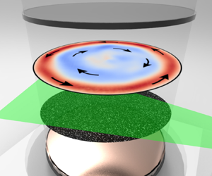
Our experimental set-up (figure 2a) consists of a cylindrical cell with height equal to the diameter 196 mm resulting in an aspect ratio of  $\varGamma =1$. The cell is cut out of a block of acrylic glass and is thus transparent from all sides. A 15 mm thick copper plate with heat conductivity 394 W m $^{-1}$ K $^{-1}$ serves as the bottom plate. It is heated via an electrical wire that is embedded in grooves at its bottom. Neighbouring grooves are 6 mm apart to enable uniform heating. Two thermistors are installed into the plate approximately 3 mm below the fluid interface. As a top plate of the convection cell, we use a 5 mm thick high-conductive sapphire plate, which is cooled by a temperature-controlled water bath. The water temperature is measured with a single thermistor and kept at a desired temperature to within $\pm 0.02$ K via a computer-controlled feedback loop.
(a) Schematic of the experimental set-up. The copper bottom plate is shown in orange; the sapphire top plate is shown in blue. (b) Investigated parameter space in an Ra–Ek plot. Different colours of the symbols show different Pr (see legend). Closed symbols mark measurements taken at  $\textit {Ra}={\rm const.}$ (datasets R1, R2, R3), while open symbols mark measurements at $\textit {Ek}={\rm const.}$ (datasets E1, E2, E3). The black solid line marks the onset of bulk convection according to Chandrasekhar (Reference Chandrasekhar1961). The solid red and blue lines mark Ra below which Coriolis forces affect the flow for the two smallest Pr. These lines are calculated based on $1/\textit {Ro}_c$ for onset of heat transport enhancement reported by Weiss et al. (Reference Weiss, Wei and Ahlers2016). Dashed lines mark Ra below which Coriolis forces become dominant over buoyancy and are estimated from the $1/\textit {Ro}_{max}$ where heat transport is maximal (Weiss et al. Reference Weiss, Wei and Ahlers2016).

The cooling water bath on top of the top plate consists of PVC sides and has a transparent top cover of acrylic glass. This transparent set-up allows optical access from the top for particle image velocimetry (PIV). For this, a Dantec RayPower 2000 laser with cylindrical lens optics is attached inside the rotating structure of the set-up as shown in figure 2(a). To measure a horizontal cross-section of the cell, the light sheet is redirected using a mirror from the side and in this way illuminates a horizontal cross-section of the cell at mid-height ( $z=H/2$). A high-speed camera (Phantom VEO4K 590-L) is mounted inside the rotating frame above the cell. For illumination, the fluid is seeded with silver-coated hollow glass spheres of diameter 10 $\mathrm {\mu }$m. Two-dimensional velocity fields were calculated from the cross-correlation of two consecutive camera snapshots, taken 20 ms apart in most cases, but this value was adapted depending on the free-fall time $\tau _{ff}$. Images were taken until the RAM of the camera (72 GB) was filled, which in all cases ensured a minimum recording time of $100\,\tau _{ff}$ (typically about 10 min). The PIV algorithm was performed with ParaPIV within MATLAB (Wang Reference Wang2018). The resulting velocity field had a resolution of $240 \times 240$ velocity points.
The entire set-up was mounted on a rotating table with a frame built on top of it and driven by a Nanotec PD4-C stepper motor. All necessary electrical connections from the lab into the rotating frame were achieved via sliprings at the top and bottom of the rotating frame. At the top, water feed-throughs were installed to supply water to the cooling water bath. The stainless steel feed-throughs were connected with bolts to the rotating frame on one side and to a non-rotating aluminum framework on the other in such a way that it kept the rotating axis fixed in space in order to avoid any precession of the set-up.
As working fluid we used mixtures of deionized water with glycerol. For most experiments, we kept the temperature constant at  $T_{m}=(T_{bot}+T_{top})/2=22.5\,^{\circ }{\rm C}$, i.e. close to room temperature, in order to minimize heat flux to or from the sides. Different Pr were achieved by using different mass concentrations of glycerol in water, which however also changes the accessible Ra and Ek ranges for a given Pr. In this paper, we focus mostly on the three cases $\textit {Pr}=6.55$ (pure water), $\textit {Pr}=12.0$ (20 % glycerol) and $\textit{Pr} \approx 76$ (60 % glycerol). By changing the temperature difference $\varDelta$ and the rotation rate $\varOmega$, we control Ra and Ek. Figure 2(b) and table 1 show an overview of the performed experiments. For each Pr, we performed measurement at fixed Ek and various Ra (E1, E2, E3) as well as measurements with one fixed Ra and varying Ek (R1, R2, R3). Due to experimental constraints, different combinations of Ek and Ra were chosen for different Pr. For two experimental runs, P1 and P2, we explored the Pr dependency of the BZF, and there we also changed $T_m$ to easily adjust Pr.
Overview of the conducted experiments.

In all measurements, we are far away from the onset of convection ( $\textit {Ra}\gg \textit {Ra}_c$), as shown in figure 2(b). Hence the observed structures close to the walls are results of strongly nonlinear interactions, in contrast to the linear wall modes close to $1/\textit {Ro}_w$. We also note that most of our measurements are not conducted in the geostrophic regime. Although it is not clear at which Ek the geostrophic regime starts, we can compare our data with heat flux measurements presented in Weiss et al. (Reference Weiss, Wei and Ahlers2016). There, the onset of heat transport enhancement was found to scale like $1/\textit {Ro}_{c1}\approx 0.75\textit {Pr}^{-0.41}$, and it presents a critical rotation rate above which Coriolis forces have a significant influence on the flow. These functions are shown as solid lines in figure 2(b). We see that all our measurements are in this regime. However, we also show as dashed lines the rotation rates $1/\textit {Ro}_{max}\approx 21.4\,\textit {Pr}^{1.37}\,\textit {Ra}^{-0.18}$, at which the heat transport was maximal (Weiss et al. Reference Weiss, Wei and Ahlers2016). Only for larger rotation rates did the Coriolis forces cause a clear suppression of the heat flux. We therefore believe that the geostrophic regime must be to the left of the dashed lines. We see that our data are in the rotation-affected regime but not in the rotation-dominated regime.
4. Results
4.1. Radial velocity profile
The horizontal velocity in Cartesian coordinates  $(u,v)$ is first transformed into polar coordinates $u_r=u\cos (\phi )+v\sin (\phi )$ and $u_{\phi }=-u\sin (\phi )+v\cos (\phi )$. Here, $r$ is the radial distance from the cell centre, and $\phi$ is the polar angle. We show in figures 3(a–d) time-averaged azimuthal velocity fields $\langle u_{\phi }(r,\phi )\rangle _t$ for different $\textit {Ek}$.
(a–d) Time-averaged  $u_{\phi }$ measured at mid-height for $\textit {Ra}=4\times 10^8$ and $\textit {Pr} \approx 76$, and $\textit {Ek}=\infty$ (a), $\textit {Ek}=6.2\times 10^{-4}$ (b), $\textit {Ek}=1.5\times 10^{-4}$ (c), and $\textit {Ek}=1.0\times 10^{-4}$ (d). (e) Red circles show the azimuthal average of (c), in physical units (left-hand $y$-axis) and normalized by the free-fall time (right-hand $y$-axis). The blue solid line is a fit of a polynomial of 10th order. The dashed vertical line marks the BZF thickness $\delta _0$, at which $\langle u_{\phi }\rangle$ crosses 0; the arrow points to the maximum velocity $u_{\phi }^{max}$ within the BZF. The inset shows results from direct numerical simulations (DNS) of the azimuthal velocity normalized by the free-fall velocity, $\langle u_{\phi }\rangle /u_{ff}$, for $\textit {Ra}=10^8$, $1/\textit {Ro}=10$, $\textit {Pr}=0.8$.

One can see how the structure of the flow changes qualitatively. In the non-rotating case ( $\textit {Ek}=\infty$), the flow field does not show a clear difference between the radial centre and the regions close to the sidewall. Instead, the distribution of the red ( $\langle u_\phi \rangle _t>0$) and blue ( $\langle u_\phi \rangle _t <0$) is orderless. In fact one would expect in this case that due to the turbulent motion, the time-averaged azimuthal velocity would be very small. This is, however, not the case, since there is a rather persistent large-scale motion, i.e. the LSC, that is steady over the time duration of our measurement. Under rotation (figures 3b–d), the characteristic features of the BZF become clearly visible, namely a red ring ( $\langle u_\phi \rangle _t >0$) surrounding a blue central region ( $\langle u_\phi \rangle _t <0$). It can be observed that with increasing rotation rates, the width of the red cyclonic zone decreases as well as the strength of the flow.
For a more quantitative analysis, we average the velocity in the azimuthal direction. For this, we sum over all velocity vectors at radial distances between  $r$ and $r+\mathrm {d}r$ away from the centre, and divide this sum by the number of voxels in this range ( $N_r$):
 \begin{equation} \langle u_{\phi}\rangle(r) = \frac{1}{N_r}\sum_{r}^{r+\mathrm{d}r}\langle u_{\phi}\rangle_t. \end{equation}
As an example, we show in figure 3(e)  $\langle u_{\phi }\rangle$ calculated from the field in figure 3(c). The red points show the calculated velocities. The blue line is a polynomial fit of degree 10 to these points that allows quantitative analysis. We also show for comparison, in the inset of figure 3(e), results from simulations at very similar $\textit {Ra}$ and $\textit {Ro}$ but smaller $\textit {Pr}=0.8$ (Zhang et al. Reference Zhang, Ecke and Shishkina2021a). At first glance, our radial profile of $\langle u_\phi \rangle$ looks very similar qualitatively to the results from direct numerical simulations (DNS). But on a closer look, quantitative differences become visible. The most obvious is the width of the BZF, i.e. the distance $\delta _0$ from the wall, where $\langle u_{\phi }\rangle$ switches sign, is much smaller in the DNS than in our case. This discrepancy is most likely due to the difference in Ek ( $1.8\times 10^{-5}$ compared to $1.5\times 10^{-4}$ for our measurement). While DNS were conducted within the rotation-dominated regime, our measurements were acquired in the rotation-affected regime. Even though Pr is different between DNS and our simulation by a factor of 10, from Zhang et al. (Reference Zhang, Ecke and Shishkina2021a) we expect no, or only a very small Pr dependency of $\delta _0$ in the investigated Pr range.
In the following, we will analyse some features of the radial profile as functions of the dimensionless control parameters. One of these features is the radial position  $r_0$, where $\langle u_{\phi }\rangle$ switches sign, i.e. where the BZF and the bulk flow separate. To be in agreement with previous publications (Zhang et al. Reference Zhang, van Gils, Horn, Wedi, Zwirner, Ahlers, Ecke, Weiss, Bodenschatz and Shishkina2020, Reference Zhang, Ecke and Shishkina2021a), we define the width of the BZF as $\delta _0=(R-r_0)/R$.
Figure 4 shows various time- and azimuthally-averaged velocity profiles for different control parameters. To compare with DNS, the velocity profiles are normalized by the free-fall velocity  $u_{ff}=\sqrt {\alpha gH\varDelta }$. In figures 4(a,c), Ra was kept constant and Ek was changed. The azimuthal velocity amplitude inside the BZF decreases with increasing rotation rate (decreasing Ek). This decrease with decreasing Ek is by no means obvious. On one hand, we know that increasing rotation suppresses fluid motion, hence a reduced velocity is expected. While this is certainly true for sufficiently fast rotation rates, for moderate rotation rates and Pr discussed here, the heat flux (Nu) is enhanced, which suggests at least a faster flow in the $z$-direction. Also note that the rate with which potential energy is converted into kinetic energy, and finally dissipated into heat, is proportional to Nu i.e. $\varepsilon _u = ({\nu ^3}/{H^4})(\textit {Nu}-1)\,\textit {Ra}\,\textit {Pr}^{-2}$. Therefore, the total kinetic energy in the fluid is expected to increase with increasing rotation rates first.
Radial profiles of  $\langle u_{\phi }\rangle$ for $\textit {Ra}={\rm const.}$ and changing Ek (a,c), and changing Ra at $\textit {Ek}={\rm const.}$ (b,d), as in the legends. (a,b) $\textit {Pr}=6.55$; (c,d) $\textit {Pr}=76$. Green dashed lines are guides to the eye and connect the velocity maxima inside the BZF measuring $\delta _{u_{\phi }^{max}}$ (see also figure 7).

The fact that we nevertheless see a decrease here for all rotation rates might be because the additional kinetic energy is contributing mostly to vertical velocity. In addition, the width of the BZF becomes smaller, hence also viscous drag would lead to a further reduction of the maximal azimuthal velocity inside the BZF.
In figures 4(b,d), Ek is kept constant and plots are shown for different Ra. The maximal velocities increase with increasing Ra, which can be explained with the enhanced thermal driving. However, we want to remind the reader that here, we show the azimuthal velocity normalized by the free-fall velocity  $u_{ff} = \sqrt {g\alpha \varDelta H} = \textit {Ra}^{1/2}(\nu \kappa )^{1/2}/H$. In fact, the Reynolds number $\textit {Re}=UH/\nu$, and hence also the typical velocity scale $U$ in non-rotating RBC, scales as $\textit {Re}\sim \textit {Ra}^{\zeta }$, with $\zeta$ determined experimentally to be in the range $\zeta \approx {0.42 \ldots 0.5}$ (see e.g. Sun & Xia Reference Sun and Xia2005; Brown, Funfschilling & Ahlers Reference Brown, Funfschilling and Ahlers2007), which would lead to $U/u_{ff}\propto \textit {Ra}^{-0.08 \,\ldots\, 0}$, i.e. a decrease with increasing Ra. Hence the azimuthal velocity in the BZF increases significantly faster with Ra than for non-rotating RBC.
In the following, we will analyse these profiles quantitatively. Most importantly, we look at the width  $\delta _0$, as well as the maximal velocity $u_\phi ^{max}$ and its location $\delta _{max}$, as functions of the control parameters Ek, Ra and Pr.
4.2. BZF width  $\delta _0$

We begin by calculating the zero-crossing and hence the thickness  $\delta _0$ as functions of the rotation rate. These results are presented in figure 5. In figure 5(a), we show $\delta _0$ as a function of $1/\textit {Ro}$ for three different $\textit {Ra}$. Note that here we have chosen to plot $1/\textit {Ro}$ on the $x$-axis, because as was shown in previous studies, different features of the heat transport seem to depend predominantly on $1/\textit {Ro}$ and depend only weakly on Ra, such as the onset of heat transport enhancement in large Pr fluids (Weiss et al. Reference Weiss, Wei and Ahlers2016) or the decrease of Nu in small Pr fluids (Wedi et al. Reference Wedi, van Gils, Bodenschatz and Weiss2021).
BZF width  $\delta _0$ as a function of the rotation rate for datasets E1 (blue circles), E2 (red squares) and E3 (green diamonds). Open symbols mark data with $1/\textit {Ro}<1/\textit {Ro}_c$. Closed symbols mark data with $1/\textit {Ro} \geq 1/\textit {Ro}_c$ (see text for further information). The error bars were estimated from the scatter of the data points around the fitted polynomial close to $\delta _0$. Panel (a) shows $\delta _0$ as a function of $1/\textit {Ro}$ on a log-log plot. The dashed lines are power-law fits to the solid symbols ( $1/\textit {Ro}\geq 1/\textit {Ro}_c$). Panel (b) shows the same data plotted against Ek. The black line is a power law $\propto \textit {Ek}^{2/3}$ as suggested by Zhang et al. (Reference Zhang, Ecke and Shishkina2021a). The purple line is a power law $\propto \textit {Ek}^{1/2}$.

We see in figure 5(a) that  $\delta _0$ decreases with increasing $1/\textit {Ro}$ for all three datasets. We have seen in figure 2(b) that our data are in the rotation-affected regime but not in the rotation-dominated regime, and that we are particularly far from the geostrophic regime for $\textit {Pr}=76$. Also considering the trend of the green data points, we decide to set a somehow arbitrary threshold for the rotation rate, which is $1/\textit {Ro}_t=1$ for $\textit {Pr}=6.55$ and $\textit {Pr}= 12.0$, and $1/\textit {Ro}_t=3$ for $\textit {Pr}=76$. In the following, we will mark data points at small and larger $1/\textit {Ro}\geq 1/\textit {Ro}_t$ with open and closed symbols, respectively, and will use only the closed symbols for scaling analysis. While this decision is somewhat arbitrary, we will see below that solid symbols often follow certain scaling relations from which the open symbols diverge. Now we fit power laws of the form $\delta _0\sim (1/\textit {Ro})^{-\alpha }$ to the data for which $1/\textit {Ro} \geq 1/\textit {Ro}_t$ (solid symbols in figure 5).
The resulting power laws are shown as dashed lines in figure 5(a) and have exponents  $\alpha _{6.55}=0.52\pm 0.03$, $\alpha _{12}=0.30\pm 0.02$ and $\alpha _{75}=0.07\pm 0.03$, with the subscript being Pr. At first glance, these three different power laws suggest that the exponent $\alpha$ is itself dependent on Ra and/or Pr, and that no simple scaling law of the form
 \begin{equation} \delta_0 =A\,\textit{Ek}^\alpha\,\textit{Ra}^\beta\,\textit{Pr}^\gamma = 2^{\alpha}A\,\textit{Ro}^\alpha\, \textit{Ra}^{\beta-\alpha/2}\,\textit{Pr}^{\gamma+\alpha/2}, \end{equation}
can be found, even though such simple scalings have been suggested recently based on numerical simulations (Zhang et al. Reference Zhang, Ecke and Shishkina2021a), namely (for  $\textit {Pr} >1$)
 \begin{equation} \delta_0 \propto \varGamma^{0}\,\textit{Pr}^{0}\,\textit{Ra}^{1/4}\,\textit{Ek}^{2/3}. \end{equation}
 For comparison with data from simulations, we plot in figure 5(b) the same measured data but now as functions of their respective Ek. Now the data for very different Ra and Pr overlap surprisingly well, for a given Ek. The black solid line in figure 5(b) is  $\propto \textit {Ek}^{2/3}$ as found in simulations by Zhang et al. (Reference Zhang, Ecke and Shishkina2021a), but is ignoring the Ra-dependency. We also show by a purple line a scaling $\propto \textit {Ek}^{1/2}$ for comparison. Here, our data seem to agree better with the purple line ( $\propto \textit {Ek}^{1/2}$), in particular for larger Ek. However, we also note that the data scatter significantly and have rather large error bars, in particular for small Ek, where the influence of buoyancy is small. Deviations from either power law occur mostly for larger Ek, where also the buoyancy becomes more important. A firm conclusion on which exponent represents the data better cannot be drawn from these data.
Clearly, there is either a simple power-law relation as in (4.2), or something more complicated as figure 5(a) suggests. In the case of a simple power-law relation (as in (4.2)), we can at least state from figure 5(b) that  $\delta _0$ might depend predominantly on Ek, but is otherwise at most very weakly dependent on Ra and Pr, at least in the range of our investigation.
Observations from DNS (see (4.3)) indeed suggest an independence from Pr, but also found an Ra-dependency  $\delta _0\propto \textit {Ra}^{1/4}$. Let us have a closer look at what our data have to say. Figure 6(a) shows $\delta _0$ as function of Ra for three different Pr and different but constant Ek. While the data with $\textit {Pr}=76$ (largest Ek) suggest a scaling of the BZF width $\delta _0\sim \textit {Ra}^\beta$ with $\beta = -{0.19\pm 0.01}$, for smaller Pr (and also smaller Ek), $\delta _0$ seems to be unaffected by Ra, i.e. $\beta \approx 0$. As before, the error bars are estimates from the scatter of the velocity data points around the fitted polynomial close to $\delta _0$. Again here, it seems that the exponent $\beta$ is a function of $\textit {Pr}$. Note in particular that for $\textit {Pr}=76$, $\delta _0$ decreases with increasing Ra, which is in disagreement with the results of DNS.
(a) Thickness  $\delta _0$ as a function of Ra for three different datasets: E1 ( $\textit {Pr}=6.55$, $\textit {Ek}=2.5\times 10^{-5}$, blue circles), E2 ( $\textit {Pr}=12.0$, $\textit {Ek}=5\times 10^{-5}$, red squares) and E3 ( $\textit {Pr}=76$, $\textit {Ek}=2\times 10^{-4}$, green diamonds). The error bars were estimated from the scatter of the data points around the fitted polynomial close to $\delta _0$. The green dashed line is a power law with exponent $\gamma =-0.19\pm 0.01$. The red and blue horizontal lines are constants with $\delta _0=0.18$ and 0.12. (b) Thickness $\delta _0$ as a function of Pr for $\textit {Ra}=6\times 10^8$ and $1/\textit {Ro}=5$ (dataset P2). The red dashed line is a power-law fit with $\sim \textit {Pr}^{0.20\pm 0.05}$. (c) Thickness $\delta _0$ as a function of Pr for $\textit {Ra}=6\times 10^8$ and $\textit {Ek}=10^{-4}$ (dataset P1). The red, orange and green lines are functions $A_1\textit {Pr}^{\gamma }$ with the values listed in table 2. The dashed blue line marks a power law $\propto \textit {Pr}^{0.1}$.

In figures 6(b,c), we show  $\delta _0$ as a function of Pr for constant Ra. Experimentally, Pr was varied by changing either $T_m$ or the concentration of glycerol in the aqueous working fluid. While it is trivial to set the system to the desired Ra by changing $\varDelta$ accordingly, the rotation rate $\varOmega$ needed to be adjusted to keep either $\textit {Ek}$ or $\textit {Ro}$ constant. We did both.
Let us first have a look at figure 6(b), where  $1/\textit {Ro}=5$. As can be seen, the data are rather noisy and do not increase strictly monotonically with Pr. There is, however, a clear trend that $\delta _0$ increases with increasing Pr, as suggested by the previous measurements. Fitting a power law of the form $\delta _0\sim \textit {Pr}^{\gamma _1}$ to the data yields $\gamma _1 =0.2\pm 0.05$.
We show in figure 6(c) values of  $\delta _0$ that were acquired at constant $\textit {Ra}$, constant $\textit {Ek}$ and varying Pr. The data scatter significantly, and no clear trend is obvious. Here, $\delta _0$ looks rather constant for small Pr, and seems to increase for larger Pr. While the red squares in figure 6(b) and the blue circles in figure 6(c) show different datasets, the data are related via (4.2). In particular, we see from (4.2) that $\gamma _1=\gamma +\alpha /2$.
We assume for a moment that  $\delta _0$ can be represented by power laws as in (4.2), but that the exponents $\alpha$, $\beta$ and $\gamma$ are different for the three different Pr ranges, as observed in figures 5(a) and 6(a). We list in table 2 the fitted parameters from figure 5(a) as well as figures 6(a,b). With this, we can calculate the expected power laws $A_1\,\textit {Pr}^{\gamma }$, with $A_1=A\,\textit {Ek}^\alpha \,\textit {Ra}^\beta$, for all three Pr ranges, which we show in figure 6(c) as solid lines. Due to the different exponents $\alpha$ for different Pr, we also get different exponents $\gamma$, which would explain the somewhat non-monotonic behaviour of the data points in figure 6(c). Indeed, the lines represent somehow the non-monotonic behaviours of the data points. Of course, assuming a power law with a varying exponent means that there is no real power law in the investigated range. However, this approach shows that the two different datasets are consistent with each other. We note that one could have also fitted a power law through the blue points in figure 6(c), resulting in a single exponent $\propto \textit {Pr}^{0.1\pm 0.03}$ (blue dashed line) over the entire range. One could then represent the data in figure 6(b) with different power laws for different Pr ranges. In any case, we have learned from figure 6(c) that (i) the Pr dependency is rather small when Ek is kept constant, and (ii) the Ra, Pr and Ek dependencies of $\delta _0$ cannot be written by simple power laws in the parameter range that we are investigating here (i.e. the rotation-affected regime).


So far we have analysed  $\delta _0$, the width of the BZF, as it can be measured easily in the time-averaged two-dimensional velocity field shown in figures 3(a–d). However, the strength of the flow, represented by the maximal averaged azimuthal velocity $u_\phi ^{max}$, is another quantity characteristic for the BZF, which can help to reveal the mechanisms leading to this zonal flow. Therefore, we show in figures 7(a,b) the compensated time-averaged maximal velocity $u^*_{max} = u_\phi ^{max}\,\textit {Ra}\,\textit {Pr}^{0.8}$, and in figures 7(c,d) its location measured as the distance from the sidewall $\delta _{max}$. These data are plotted against $\textit {Ra}\,\textit {Ek}$ on the $x$-axis, as this represents the Rayleigh number compared to its critical value for the onset of wall modes ( $\textit {Ra}_w\propto \textit {Ek}^{-1}$). We show in figures 7(a,c) data that were acquired at constant $\textit {Ek}$ for a given Pr and varying Ra, whereas figure 7(b,d) show data with constant Ra and different Ek.
(a,b) Compensated maximal averaged azimuthal velocity  $u_{\phi }^{max}\,\textit {Ra}\,\textit {Pr}^{0.8}$ as a function of Ek Ra. (a) Data acquired at constant Ek (datasets E1, E2, E3). (b) Data acquired at constant Ra (datasets R1, R2, R3). The solid black lines in (a) and (b) mark the same power law $\propto (\textit {Ek}\,\textit {Ra})^{3/2}$. (c,d) Distance between the sidewall and the location of the azimuthal velocity maximum $\delta _{u_{\phi }^{max}}$. (c) Datasets E1, E2, E3 with constant Ek. (d) Datasets R1, R2, R3 taken at constant Ra. Open symbols in (b) and (d) mark data with $1/\textit {Ro}<1/\textit {Ro}_t$ (see text). The inset in (c) shows the same data but plotted without the normalization $\textit {Ek}^{-1/2}$. One sees that the data do not collapse on top of each other. The blue arrow in (c) marks the estimated location of the maximal heat transport for dataset E1.

Let us first have a look at the compensated maximal averaged azimuthal velocity  $u^*_{max}$ shown in figure 7(a). Note that the definition of $u^*_{max}$ is not based on scaling arguments, but is rather an empirical relation that provides a very good collapse of data onto a single power law for all three Pr, with each having a different Ek. The black solid line marks $u^*_{max}= 4.7(\textit {Ek}\,\textit {Ra})^{3/2}$ (or equivalently $u_\phi ^{max} = 4.7\,\textit {Ek}^{3/2}\,\textit {Ra}^{1/2}\,\textit {Pr}^{-0.8}$), which represents the data fairly well. We show the same function as a black line also in figure 7(b), but now compare it with measurements that were acquired at constant Ra but varying Ek. We see that data for small values of Ek Ra follow this law, but data for large values of Ek Ra diverge from the straight line. For a better visual separation, data with $1/\textit {Ro}\geq 1/\textit {Ro}_t$ were plotted with solid symbols, whereas data for which $1/\textit {Ro}<1/\textit {Ro}_t$ were plotted with open symbols. As mentioned previously, we assumed $1/\textit {Ro}_t=1$ for the two smaller Pr, and $1/\textit {Ro}_t=3$ for $\textit {Pr}=76$. Since data for varying Ra follow the mentioned power law for nearly two decades, we are confident that this power law also holds for smaller $\textit {Ek}$, at least as long as buoyancy plays a significant role. Whether this scaling holds even in the rotation-dominated regime, however, remains unclear.
Figures 7(c,d) show the distance from the wall to the maximal velocity  $\delta _{max}$, normalized by $\sqrt {\textit {Ek}}$ and plotted against $\textit {Ek}\,\textit {Ra}$. Measurements are the same as for figures 7(a,b), which means constant $\textit {Ek}$ for figure 7(c), and constant Ra for figure 7(d). We see that the data collapse fairly well on a constant $\delta _{max}/\sqrt {\textit {Ek}}\approx 10$ or so. The inset in figure 7(c) shows that data do not collapse on top of each other without this normalization. However, the green data points ( $\textit {Pr}=76$) seem to decrease slightly for larger Ek Ra, which might hint at the fact that buoyancy becomes too strong compared to Coriolis forces.
In figure 7(d), the same quantity is plotted but from data where Ra was constant (for a given Pr) and Ek was varied. We again plot with solid symbols data with  $1/\textit {Ro} \geq 1/\textit {Ro}_t$, and use open symbols for data with $1/\textit {Ro}<1/\textit {Ro}_t$. Clearly, the overlap of data with different Pr is rather good only for sufficiently large $1/\textit {Ro}$ (solid symbols), and less good for the open symbols.
Data plotted as  $\delta _{max}/\sqrt {\textit {Ek}}$ (see figures 7c,d) collapse onto a single flat line, suggesting that $\delta _{max} \propto \textit {Ek}^{1/2}$ and $\delta _{max}$ otherwise independent of Ra and Pr. We have already seen above (figure 5) that a similar scaling might also be visible in the data for $\delta _0$, the thickness of the BZF. In fact, in figure 5(b), we have plotted already a purple line marking a power law $\delta _0\propto \textit {Ek}^{1/2}$. Now, for a better comparison, we plot in figure 8(a) both $\delta _{max}/\sqrt {\textit {Ek}}$ and $\delta _0/\sqrt {\textit {Ek}}$ as open and solid symbols inside the same graph. Clearly, the scatter of the data for $\delta _0$ is much larger, but both follow straight lines over more than a decade in Ek Ra. However, in both cases, the green data ( $\textit {Pr}=76$) for the largest Ek Ra clearly decrease.
(a) Normalized length scales  $\delta _0/\sqrt {\textit {Ek}}$ (closed symbols) and $\delta _{max}/\sqrt {\textit {Ek}}$ (open symbols) as functions of $\textit {Ek}\,\textit {Ra}$. Note that data are presented for datasets E1, E2 and E3, where in fact only Ra was varied. The straight black lines mark $\delta _0/\sqrt {\textit {Ek}}=24.0$ and $\delta _{max}/\sqrt {\textit {Ek}}=9.2$. (b) Ratio $\delta _0/\delta _{max}$ as function of $\textit {Ek}\,\textit {Ra}$. Here, the open (closed) symbols are datasets with constant (varying) Ra and varying (constant) Ek. The different colours denote the different Prandtl numbers $\textit {Pr}=6.55$ (blue circles), 12 (red squares), 76 (green diamonds). The straight black line marks $\delta _0/\delta _{max}=2.6$.

Figure 8(b) shows the ratio  $\delta _0/\delta _{max}$ as a function of Ek Ra. For this we have used all available data, and show data with constant Ek as open symbols, and data with constant Ra as solid symbols. The colour marks Pr. It becomes evident that the ratio $\delta _0/\delta _{max}\approx 2.6$ is a constant, therefore both $\delta _0$ and $\delta _{max}$ should exhibit the same scaling relations with the control parameters. However, we note that due to the rather large scattering of the data, small differences in the scaling exponents cannot be ruled out.
5. Conclusion
In this paper, we have presented measurements of the horizontal velocity at mid-height in a rotating Rayleigh–Bénard cell of aspect ratio  $\varGamma =1$ for various Ra, Ek and Pr using planar PIV. In these measurements, we could observe the boundary zonal flow (BZF) for the first time in an experiment, as a ring with positive average azimuthal velocity $\langle u_{\phi }\rangle > 0$ (cyclonic motion) surrounding a central region with $\langle u_{\phi }\rangle < 0$ (anticyclonic motion) as reported in Zhang et al. (Reference Zhang, van Gils, Horn, Wedi, Zwirner, Ahlers, Ecke, Weiss, Bodenschatz and Shishkina2020, Reference Zhang, Ecke and Shishkina2021a).
We studied the thickness of this zone ( $\delta _0$) as a function of Ek, Ra and Pr. Interpretation of the measured data is a somewhat difficult task, because on the one hand, the available parameter ranges cover no more than a decade, but also because we cover mainly small rotation rates, where the system is in the rotation-affected regime, where buoyancy is small compared to Coriolis forces. Hence it is unclear whether simple scaling laws are even expected in this regime and whether they will hold also in the rotation-dominated (geostrophic) regime. For example, for sufficiently large rotation rates (i.e. $1/\textit {Ro} > 1/\textit {Ro}_t$), $\delta _0$ seems to follow $\propto 1/\textit {Ro}^{\alpha }$, with $\alpha (\textit {Pr})$ being a function of Pr. While such a relation is possible (see e.g. Grossmann & Lohse Reference Grossmann and Lohse2000, Reference Grossmann and Lohse2001), finding the correct function $\alpha (\textit {Pr})$ is a difficult task for which many more data points over a much larger range need to be acquired to get reliable results.
Furthermore, we know that the rotation-affected regime as well as the rotation-dominated regime consists of smaller sub-regimes with transitions between them, as has been observed in measurements of the vertical heat flux (see e.g. Zhong & Ahlers Reference Zhong and Ahlers2010; Wei et al. Reference Wei, Weiss and Ahlers2015) and the flow configuration in the bulk (e.g. Stellmach et al. Reference Stellmach, Lischper, Julien, Vasil, Cheng, Ribeiro, King and Aurnou2014; Plumley et al. Reference Plumley, Julien, Marti and Stellmach2016). In which way these regimes affect properties of the BZF is currently unclear. While it is somehow expected that transitions in the bulk from one regime to another also change how the BZF properties depend on Ra, Ek and Pr, it is also possible that the BZF is decoupled from the dynamics in the bulk for sufficiently large rotation rates. As a result, scaling relations of its properties could hold in both the rotation-affected and rotation-dominated regimes. In this context, we want to remind the reader that data for  $\textit {Pr}=6.55$ (datasets E1 and R1) cover not only parameter ranges, where a heat transport enhancement has been observed, but also ranges where a heat transport reduction is expected (see Zhong & Ahlers Reference Zhong and Ahlers2010; Weiss et al. Reference Weiss, Wei and Ahlers2016). In fact, the location of maximal heat transport enhancement for dataset E1 is marked with a blue arrow in figure 7(c). The trends of both $u_{\phi }^{max}$ and $\delta _{max}$ do not show significant differences at the left (Nu reduction) and the right (Nu enhancement) of this arrow.
Under the assumption of a simple power-law relationship of the form  $\delta _0\propto \textit {Ek}^\alpha \textit {Ra}^\beta \textit {Pr}^{\gamma }$, our data suggest $\beta \approx 0$ or close by. In fact, only for the largest number, $\textit {Pr}=76$, do we find a slight decrease of $\delta _0$ with increasing Ra, which might be due to insufficient rotation rates. This exponent is in contrast to $\beta =1/4$, as found in numerical simulations by Zhang et al. (Reference Zhang, Ecke and Shishkina2021a). The exponent $\gamma$ is around zero, or at least very small, which is in agreement with the scaling found in DNS, at least in the same Pr range (Zhang et al. Reference Zhang, Ecke and Shishkina2021a). Regarding the $\textit {Ek}$ scaling, our data suggest $\alpha \approx {1/2}$, again in contrast to DNS (Zhang et al. Reference Zhang, Ecke and Shishkina2021a), where $\alpha =2/3$ was suggested. A possible explanation for the difference between DNS and our experiment is the different parameter ranges. In fact, Zhang et al. (Reference Zhang, Ecke and Shishkina2021a) report results for $\textit {Pr}>1$ only for cylinders of aspect ratio $\varGamma =1/2$. However, probably more important for the datasets of comparable Pr is that Ek in DNS is at least an order of magnitude smaller, and therefore Coriolis forces are much stronger compared to buoyancy in the simulation. It is indeed possible that the scaling relations that we find change for faster rotation and converge towards the findings in DNS.
In this respect, we note that in DNS, different scaling relations were found for  $\delta _0$ and $\delta _{max}$, i.e. the distance from the sidewall at which the averaged azimuthal velocity is maximal. Here we find that both scale similarly $\propto \textit {Ek}^{1/2}$. The maximal azimuthal velocity itself is found in our measurements to scale as $u_\phi ^{max}\propto \textit {Ek}^{3/2}\,\textit {Ra}^{1/2}\,\textit {Pr}^{-0.8}$. It is interesting that both $\delta _{max}$ and $\delta _0$ are independent of Ra, but $u_\phi ^{max}$ is not, suggesting that different mechanisms play a role here. In particular, the width is not just a result of a self-adjusting wall shear stress. Note in this respect that in this system, $\textit {Ek}\,\textit {Ra}$ represents the amount of thermal driving, compared to the minimal buoyancy that is necessary to initiate wall modes. On the other hand, $\delta _{max}$ and $\delta _0$ are self-adjusting purely by Coriolis forces. To investigate this problem further, more measurements and simulations are necessary that indeed cover the entire range from the onset of wall modes up to the buoyancy-dominated regime.
Acknowledgements
We thank Olga Shishkina and Xuan Zhang for fruitful discussions. We also acknowledge support by Eberhard Bodenschatz for providing technical and administrative infrastructure for this project.
Funding
We acknowledge financial support by the Deutsche Forschungsgemeinschaft (DFG) through grant WE 5011/4-1, and from the European High-Performance Infrastructure in Turbulence programme (EuHIT). D.F. received a travel grant from the Deutscher Akademischer Austauschdienst (DAAD).
Declaration of interests
The authors report no conflict of interests.


 Open access