


1. Introduction
Collisionless shocks are one of the most ubiquitous phenomena in space plasmas, and one of the most studied nonlinear plasma systems during the last seventy years. While the primary interest in collisionless shocks is related to their being among the most powerful accelerators of charged particles in remote astrophysical objects, like supernova remnants, or at the large scale of clusters of galaxies, the heliosphere is the only natural laboratory where these shocks can be studied in detail with in situ measurements. All mentioned shocks are non-relativistic magnetized fast shocks, in which the magnetic field plays a major role and the shock speed exceeds the fast magnetosonic speed. The shock structure, that is, the magnetic field inside the shock transition, and the corresponding particle motion and distributions, are the focus of the heliospheric shock studies. It is well known that the magnetic profile of fast shocks evolves with the increase of the Mach number. The concept of a shock has been born within magnetohydrodynamics (MHD), where it is treated as a discontinuity. In what follows we shall extensively use the normal incidence frame (NIF). The NIF is the frame in which a shock discontinuity stands and the plasma flow enters the shock along the shock normal with the velocity $V_u$ (the upstream NIF velocity). Hereafter, subscript $u$
 means ‘upstream’ and subscript $d$
 means ‘downstream’, in the shock frame. In MHD, fast shocks are typically characterized by the angle $\theta _{Bn}$
 between the upstream magnetic field vector $\boldsymbol {B}_u$
 and the normal to the shock front $\hat {\boldsymbol {n}}$
 . The latter will be assumed to point from the upstream to the downstream. A shock is also characterized by the parameter $\beta _u=8{\rm \pi} p_u/B_u^2$
 , where $p_u$
 is the upstream kinetic plasma pressure. The most important shock parameter is the Mach number. The Alfvénic Mach number is $M_A$
 and the fast Mach number $M_F$
 are defined as follows:


where $n_u$ is the upstream proton number density, $m_p$
 is the proton mass and $v_s$
 is the sound speed. For simplicity, the plasma is considered to consist of protons and electrons, while possible admixtures of $\alpha$
 -particles are ignored. The sound speed $v_s^2=\gamma T_u/m_p$
 , where $T_u=p_u/n_u$
 is the upstream temperature, and $\gamma =5/3$
 in isotropic plasmas. For fast shocks $M_A>M_F>1$
 . The magnetic profile of a shock depends on all three parameters, $M_A$
 , $\theta _{Bn}$
 and $\beta _u$
 . Magnetic profiles or quasi-perpendicular shocks, $\theta _{Bn}>45^\circ$
 , are typically more regular than that of quasiparallel shocks, $\theta _{Bn}<45^\circ$
 (Bale et al. Reference Bale, Balikhin, Horbury, Krasnoselskikh, Kucharek, Möbius, Walker, Balogh, Burgess and Lembège2005; Burgess et al. Reference Burgess, Lucek, Scholer, Bale, Balikhin, Balogh, Horbury, Krasnoselskikh, Kucharek and Lembège2005; Krasnoselskikh et al. Reference Krasnoselskikh, Balikhin, Walker, Schwartz, Sundkvist, Lobzin, Gedalin, Bale, Mozer and Soucek2013). Low $\beta _u$
 shocks are typically less structured than high $\beta _u$
 shocks (Greenstadt et al. Reference Greenstadt, Scarf, Russell, Formisano and Neugebauer1975, Reference Greenstadt, Russell, Formisano, Hedgecock, Scarf, Neugebauer and Holzer1977, Reference Greenstadt, Russell, Gosling, Bame, Paschmann, Parks, Anderson, Scarf, Anderson and Gurnett1980; Russell et al. Reference Russell, Hoppe, Livesey, Gosling and Bame1982b; Farris, Russell & Thomsen Reference Farris, Russell and Thomsen1993). However, the Mach number is usually considered the main parameter related to structural changes of the collisionless shock front. The Alfvénic Mach number has a simple physical meaning: the ratio of the kinetic energy flux along the shock normal $n_um_pV_u^3$
 to the Poynting flux $c(\boldsymbol {E}\times \boldsymbol {B})\boldsymbol {\cdot }\hat {\boldsymbol {n}}/4{\rm \pi} =V_uB_u^2/4{\rm \pi}$
 is $M_A^2$
 . The fast Mach number does not have such a simple energetic meaning, so we usually use $M_A$
 . Low $M_A$
 low $\beta _u$
 shocks are laminar, with nearly monotonically increasing magnetic field magnitude. The dissipative MHD relates changes in the structure to the absence of shock solutions with resistivity and thermal conduction alone above the so-called critical Mach number, at which the downstream flow velocity along the shock normal drops below the downstream sound speed (Kennel Reference Kennel1987, Reference Kennel1988). Above the critical Mach number, viscosity is necessary. This critical Mach number is often considered to mark the onset of ion reflection. However, theoretically, ion reflection and the accompanying appearance of overshoot and downstream magnetic oscillations were predicted for dispersive shocks, where above some critical Mach number a soliton solution is not possible (Sagdeev Reference Sagdeev1966). The two critical Mach numbers are different, the dissipative one being smaller than the dispersive one (Forslund & Freidberg Reference Forslund and Freidberg1971; Manheimer & Spicer Reference Manheimer and Spicer1985). Yet, traditionally deviation from the monotonic shape and onset of ion reflection was attributed to crossing the dissipative critical Mach number (Livesey, Kennel & Russell Reference Livesey, Kennel and Russell1982; Russell, Hoppe & Livesey Reference Russell, Hoppe and Livesey1982a), and up to now shocks are often classified as subcritical or supercritical (Zhou & Smith Reference Zhou and Smith2015). It was found observationally that ion reflection and overshoot occur in subcritical shocks as well (Farris et al. Reference Farris, Russell and Thomsen1993). It has been shown, observationally, theoretically and in simulations, that even in very low Mach number shocks overshoot and downstream magnetic oscillations develop due to the transmitted ion gyration and slow gyrophase mixing and kinematic collisionless relaxation (Balikhin et al. Reference Balikhin, Zhang, Gedalin, Ganushkina and Pope2008; Ofman et al. Reference Ofman, Balikhin, Russell and Gedalin2009; Gedalin Reference Gedalin2015; Gedalin, Friedman & Balikhin Reference Gedalin, Friedman and Balikhin2015). Overshoots are stronger in higher Mach number shocks (Livesey et al. Reference Livesey, Kennel and Russell1982; Russell et al. Reference Russell, Hoppe and Livesey1982a; Tatrallyay, Luhmann & Research Reference Tatrallyay, Luhmann and Research1984; Scudder et al. Reference Scudder, Aggson, Aggson, Mangeney, Lacombe and Harvey1986; Mellott & Livesey Reference Mellott and Livesey1987; Tatrallyay et al. Reference Tatrallyay, Gevai, Apathy, Schwingenschuh, Zhang, Kotova, Verigin, Livi and Rosenbauer1997; Masters et al. Reference Masters, Slavin, Dibraccio, Sundberg, Winslow, Johnson, Anderson and Korth2013), which was thought, until recently, due to reflected ions. Low Mach number shocks are planar and time stationary, to a very good approximation. Even at rather high Mach numbers, a shock may be planar and time stationary (Scudder et al. Reference Scudder, Aggson, Aggson, Mangeney, Lacombe and Harvey1986). It was shown that, in moderately supercritical shocks, the magnetic profile is consistent with the kinematic collisionless relaxation and may be only weakly non-planar or time-dependent (Gedalin Reference Gedalin2019a,Reference Gedalinb,Reference Gedalinc). At sufficiently high Mach numbers, shocks become rippled (Moullard et al. Reference Moullard, Burgess, Horbury and Lucek2006; Lobzin et al. Reference Lobzin, Krasnoselskikh, Musatenko and Dudok de Wit2008; Ofman & Gedalin Reference Ofman and Gedalin2013; Johlander et al. Reference Johlander, Schwartz, Vaivads, Khotyaintsev, Gingell, Peng, Markidis, Lindqvist, Ergun and Marklund2016; Gingell et al. Reference Gingell, Schwartz, Burgess, Johlander, Russell, Burch, Ergun, Fuselier, Gershman and Giles2017; Johlander et al. Reference Johlander, Vaivads, Khotyaintsev, Gingell, Schwartz, Giles, Torbert and Russell2018) or reforming (Lobzin et al. Reference Lobzin, Krasnoselskikh, Bosqued, Pinçon, Schwartz and Dunlop2007; Lefebvre et al. Reference Lefebvre, Seki, Schwartz, Mazelle and Lucek2009; Tiu et al. Reference Tiu, Cairns, Yuan and Robinson2011; Sundberg et al. Reference Sundberg, Boardsen, Slavin, Uritsky, Anderson, Korth, Gershman, Raines, Zurbuchen and Solomon2013; Dimmock et al. Reference Dimmock, Russell, Sagdeev, Krasnoselskikh, Walker, Carr, Dandouras, Escoubet, Ganushkina and Gedalin2019; Liu et al. Reference Liu, Hao, Wilson III, Turner and Zhang2021). It was suggested that onset of time dependence occurs when the so-called whistler critical Mach number is exceeded (see, e.g. Krasnoselskikh et al. Reference Krasnoselskikh, Balikhin, Walker, Schwartz, Sundkvist, Lobzin, Gedalin, Bale, Mozer and Soucek2013), and the upstream whistler waves can no longer stand in the shock frame.
All the above approaches, striving to explain the observed structural changes in the magnetic profile with the increase of the Mach number, focus on nonlinear wave features or details of the ion dynamics. Indeed, ions carry most of mass, momentum and energy, and therefore ions shape the profile. However, we suggest that the kind of shock structure (laminar, planar and stationary structured, rippled, reforming or whatever else will be observed in the future) is independent of the exact mechanism causing the structure, and is determined by the necessity to ensure stable transfer of mass, momentum and energy across the shock. By stable we mean that on average the fluxes of the above-mentioned conserved quantities should be constant and there should be no large disruptions in the transfer. We suggest that a collisionless shock is a self-regulatory system, and the shock structure is the one that ensures the stability of the mass, momentum and energy fluxes, for given upstream parameters. Within this approach, the focus is shifted from reason to purpose: more than one microscopic process may lead to the same type of collisionless shock structure, which is determined solely by the requirement of stable fluxes. In other words, this means that if the conservation laws can be fulfilled with a laminar profile, the shock will be laminar. With the increase of the Mach number, this is no longer possible, and the shock develops a structure, no matter what it is the mechanism of the structure generation. It has been shown that, in higher Mach number shocks, necessary ion heating requires stronger ion reflection, which in turn requires the development of an overshoot (Gedalin et al. Reference Gedalin, Dimmock, Russell, Pogorelov and Roytershteyn2023a). The mechanism of the overshoot formation is due to the deceleration of the transmitted ion flow, while the reflected ions limit overshoot growth, thus ensuring stability (Gedalin & Sharma Reference Gedalin and Sharma2023; Sharma & Gedalin Reference Sharma and Gedalin2023). Here, we show that, at even higher Mach numbers, a planar stationary structure cannot ensure stable mass, momentum and energy conservation, which means that the shock front becomes rippled.
2. Observations
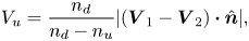
In this section, we describe observations of a shock which is modelled in the rest of the paper. Figure 1 shows the magnitude and three components of the magnetic field, measured by MMS1 on 22 April 2020 at 16:43:50 UTC. The resolution corresponds to the FGM survey mode (Russell et al. Reference Russell, Anderson, Baumjohann, Bromund, Dearborn, Fischer, Le, Leinweber, Leneman and Magnes2016; Torbert et al. Reference Torbert, Russell, Magnes, Ergun, Lindqvist, Le Contel, Vaith, Macri, Myers and Rau2016). The fields are rotated into the shock coordinates, as follows: the $x$ -coordinate is along the model shock normal (Farris & Russell Reference Farris and Russell1994), $\hat {\boldsymbol {n}}=(0.6720, -0.7152, 0.1921)$
 in the GSE coordinates, pointing toward downstream, the $z$
 -coordinate is along the difference between the downstream and upstream magnetic field vectors $\Delta \boldsymbol {B}=\boldsymbol {B}_d-\boldsymbol {B}_u$
 and the non-coplanarity direction is $\hat {\boldsymbol {y}}=\hat {\boldsymbol {z}}\times \hat {\boldsymbol {x}}$
 . The upstream region is chosen visually as $-166 < t <-86$
 (in seconds from the crossing), and the downstream region is $212< t<447$
 . The angle between the upstream magnetic field and the shock normal $\theta _{Bn}=115^\circ$
 . The magnetic compression ${B_d/B_u=2.9}$
 . The upstream and downstream ions and electron number densities $n_{iu}=3.0$
 cm$^{-3}$
 , $n_{eu}=2.3$
 cm$^{-3}$
 , $n_{id}=9.7$
 cm$^{-3}$
 and $n_{ed}=9.8$
 cm$^{-3}$
 are taken from plasma measurements by FPI (Pollock et al. Reference Pollock, Moore, Jacques, Burch, Gliese, Omoto, Avanov, Barrie, Coffey and Dorelli2016). The upstream densities differ, although quasi-neutrality is supposed to hold. The Alfvén speed, the shock speed and the upstream plasma velocity in NIF are calculated as


where $\boldsymbol {V}_1$ and $\boldsymbol {V}_2$
 are the plasma velocities in the upstream and downstream regions, as measured by the spacecraft. When using the electron velocities $\boldsymbol {V}_{e1}\boldsymbol {\cdot }\hat {\boldsymbol {n}}=301.5\,\text {km}\,\text {s}^{-1}$
 , $\boldsymbol {V}_{e2}\boldsymbol {\cdot }\hat {\boldsymbol {n}}=76.0\,\text {km}\,\text {s}^{-1}$
 and densities in (2.1)–(2.3), the shock speed has a wrong sign, so we use the ion velocities $\boldsymbol {V}_{i1}\boldsymbol {\cdot }\hat {\boldsymbol {n}}=291.0\,\text {km}\,\text {s}^{-1}$
 , $\boldsymbol {V}_{i2}\boldsymbol {\cdot }\hat {\boldsymbol {n}}=76.5\,\text {km}\,\text {s}^{-1}$
 , which give $v_A\approx 38\,\text {km}\,\text {s}^{-1}$
 , $V_u\approx 308\,\text {km}\,\text {s}^{-1}$
 and $M_A=V_u/v_A\approx 8$
 . The upstream $\beta _{iu}=7.8$
 and $\beta _{eu}=6.1$
 , as calculated onboard. For $\beta _u\approx 10$
 the fast Mach number $M_F\approx 2.5$
 . In what follows we use the upstream ion gyrofrequency $\varOmega _u=eB_u/m_pc$
 and the ion inertial length $c/\omega _{pi}$
 , $\omega _{pi}^2=4{\rm \pi} n_ue^2/m_p$
 .
.
The magnitude and three components of the magnetic field, measured by MMS1 on 22 April 2020 at 16:43:50 UTC. The components are given in the shock frame, see details in the text.
The non-coplanar component of the magnetic field $B_y$ makes excursion toward negative values inside the central part of the transition, in qualitative agreement with the theoretically derived relation $B_y\propto \cos \theta _{Bn}({\rm d} B_z/{\rm d} z)$
 (see, e.g. Gedalin et al. Reference Gedalin, Golbraikh, Russell and Dimmock2022). On the other hand, the strong fluctuations of $B_x$
 inside the central part clearly indicate the non-planarity of the shock front (Gedalin & Ganushkina Reference Gedalin and Ganushkina2022). The maximum magnetic field is $B_m/B_u\approx 6.7$
 . The tangential components of the upstream plasma velocity in the spacecraft frame are $V_{y}\approx 130$
 km s$^{-1}$
 and $V_{z}\approx -260$
 km s$^{-1}$
 . The shock speed in the spacecraft frame is $V_{sh}\approx -17$
 km s$^{-1}$
 . This means that the spacecraft crosses the shock tangentially, at an angle ${\approx }87^\circ$
 to the shock normal, and at an angle ${\approx }27^\circ$
 to $z$
 -direction.
3. Modelling
The principles of the approach are as follows: we numerically trace ions across a model shock front, derive the total pressure $p_{xx}=m_p\langle \int v_x^2f(\boldsymbol {r},\boldsymbol {v},t)\,{\rm d}^3\boldsymbol {v} \rangle$ of the generated ion distribution and analyse whether this pressure is consistent with the model shock profile used for the tracing. Here, $f(\boldsymbol {r},\boldsymbol {v},t)$
 is the ion distribution function, and $\langle (\cdots )\rangle$
 denotes proper spatial and temporal averaging, if such is needed. In this approach, mass conservation is fulfilled automatically. We restrict ourselves to one component of the pressure only. A more sophisticated approach, taking into account also $p_{yx}$
 , $p_{zx}$
 and the energy flux, would be beyond any possible precision of the model. Initially, ions are distributed according to the Maxwellian distribution with the thermal speed $v_T=V_u\sqrt {\beta _{iu}/2}/M_A$
 . The method was described in detail by Gedalin (Reference Gedalin2016). The electron pressure is taken into account in the adiabatic approximation $p_e/n^{5/3}=\text {const}$
 . Note that we are not going to reproduce the profile or any of the details of the shock described in § 2. Given the uncertainties of measurements and errors in the determination of the shock parameters, this task would be impossible. The objective of the present study is to analyse whether a shock with the parameters in the observed range, that is, a quasi-perpendicular high Mach number, high-$\beta$
 shock can be laminar or structured planar stationary, or the stability of the fluxes of the conserved quantities dictate non-planarity and dependence on time (rippling).
3.1. Non-structured profile
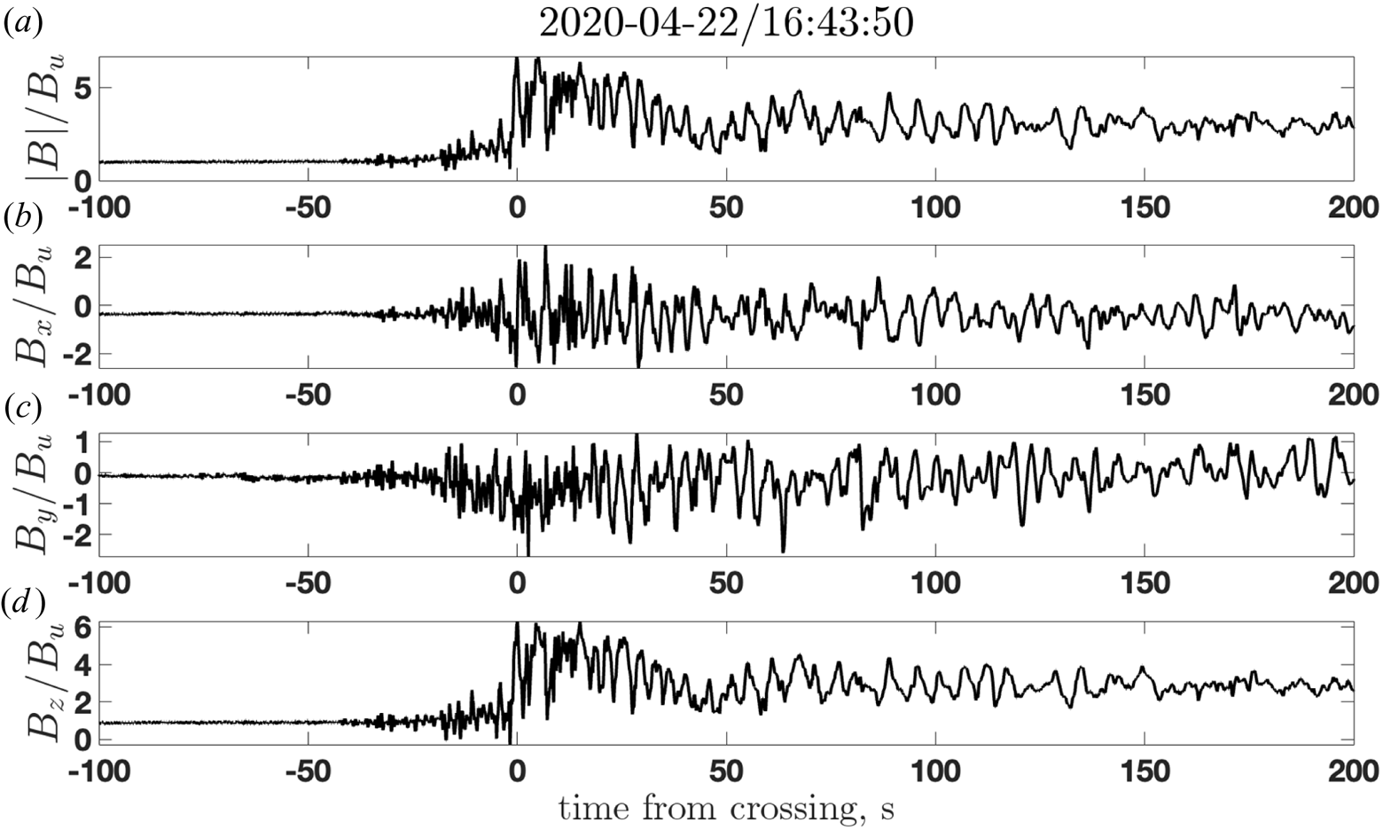
We start with the attempt to model the observed shock with a laminar profile with the calculated magnetic compression of $B_d/B_u=2.9$ . Figure 2 presents the magnetic compression $B_d/B_u$
 as a function of the Alfvénic Mach number $M_A$
 , obtained by solving the Rankine–Hugoniot relations (Kennel et al. Reference Kennel, Edmiston and Hada1985) for various upstream $\beta _u$
 . For a given $B_d/B_u$
 , higher $\beta _u$
 requires higher $M_A$
 . It is seen that the measured $B_d/B_u$
 and $\beta _u$
 are inconsistent with the derived Mach number. Since the Rankine–Hugoniot relations are nothing but conservation laws and must be fulfilled, we will choose $B_d/B_u=2.8$
 , $\beta _u=12$
 and $M_A=10$
 for the modelling.
The magnetic compression $B_d/B_u$ as a function of the Alfvénic Mach number $M_A$
 , for various $\beta _u$
 , as obtained from the solution of the Rankine–Hugoniot relations (Kennel, Edmiston & Hada Reference Kennel, Edmiston and Hada1985).
We start with a monotonic magnetic field given by the expressions


The expression (3.3) has been derived within a two-fluid study of stationary nonlinear waves (Gedalin Reference Gedalin1998). These expressions should be completed with the electric field, which takes the form: $E_z=0$ , $E_y=V_uB_u\sin \theta _{Bn}/c$
 and $E_x=-K_E B_y$
 . The coefficient $K_E$
 is determined by the value of the cross-shock potential

where $s$ is one of the varied parameters of modelling. The ramp width is chosen as ${D=c/\omega _{pi}}$
 .
.
Figure 3 presents the reduced distribution function $f(x,v_x)=\int f(x,\boldsymbol {v})\,{\rm d} v_y\,{\rm d} v_z$ . Heating occurs mainly due to the downstream gyration of the directly transmitted ions. Reflected ions contribute a small part. The kinematic collisionless relaxation due to the gyrophase mixing is seen very clearly. The decisive step is the calculation of the magnetic field from the conservation law

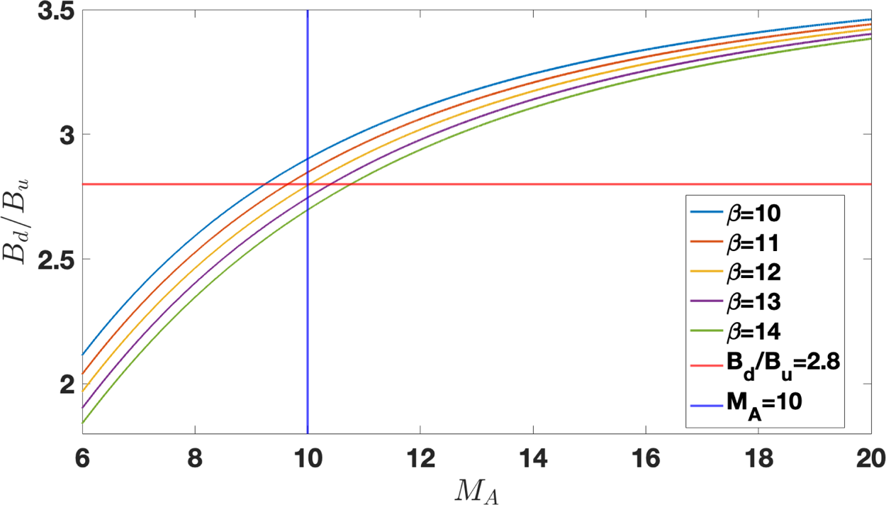
where $n=\int f(x,v_x)\,{\rm d} v_x$ . This magnetic field is shown in figure 4. It is seen that the calculated magnetic field approaches the model magnetic field well behind the shock transition. It should be mentioned that the result is sensitive to the value of $s$
 . At first sight, the model is successful. However, in a planar stationary shock the equation (3.6) should be valid throughout the shock, for each position $x$
 . However, figure 4 shows that (3.6) requires that the shock profile be structured. In particular, the shock structure should include a large overshoot. We, therefore, move on to modelling a structured planar stationary shock. Such shocks were shown to exist (Scudder et al. Reference Scudder, Aggson, Aggson, Mangeney, Lacombe and Harvey1986).


The magnetic field calculated from (3.6).
3.2. A structured planar stationary shock model
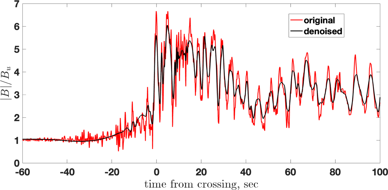
Our objective is to model a structured shock profile, which would include at least a foot and an overshoot and would be similar to the observed shock profile, but not necessarily reproduce the latter. Such modelling requires first denoising the magnetic profile, that is, removing oscillations that are supposed not to be a part of the shock structure but, possibly, transient waves or observed due to the tangential crossing of the shock by the spacecraft. Figure 4 makes the impression that at least one magnetic maximum corresponds to the overshoot, after which the magnetic field drops to the downstream value or below it. The position of the overshoot corresponds to the position of the maximal deceleration of the directly transmitted ions in figure 3. Figure 3 also shows that the reflected ions appear as far as approximately $0.5(V_u/\varOmega _u)$ from the ramp. This distance should approximately correspond to the foot length of a structured shock. Figure 5 compares the original profile with a denoised one. The latter is obtained by applying Daubechies 10 wavelet transform, reducing the smaller scale 9 levels, and applying the inverse transform (WaveShrink procedure of the WaveLab 850 package).
The original magnetic field magnitude truncated to $2^{13}$ points (red) and the denoised magnetic field. The denoising is done by applying Daubechies 10 wavelet transform, reducing the smaller scale 9 levels, and applying the inverse transform.
An overshoot is added as follows:


For the run below the following parameters are chosen: $a=1$ , $w_l=0.3(V_u/\varOmega _u)$
 , $w_r=1.87(V_u/\varOmega _u)$
 , $x_l=0.1(V_u/\varOmega _u)$
 , $x_r=0.15(V_u/\varOmega _u)$
 . Because of the overshoot, the cross-shock potential has to be modified, so the downstream value $s_d=0.2$
 while ${s_{\max }=0.35}$
 .
.
Figure 6 shows the reduced distribution function $f(x,v_x)$ , in the format similar to figure 3. It has been shown that an overshoot enhances ion reflection (Gedalin et al. Reference Gedalin, Dimmock, Russell, Pogorelov and Roytershteyn2023a). This enhancement is easily seen comparing figures 3 and 6. Ion reflection is strong because of the large $v_T/v_u=0.17$
 (Sharma & Gedalin Reference Sharma and Gedalin2023). The much larger fraction of the reflected ions in the structured shock reverses the behaviour of the total ion pressure $p_{xx}$
 across the shock from decreasing, as required by the conservation laws, to increasing, which is impossible in a stable shock. Although figure 7 shows this behaviour for one set of parameters but it has been found that no variation of parameters can reduce the far downstream $p_{xx}$
 to below the upstream value. Thus, the observed profile (figures 1 and 5) cannot belong to a planar stationary shock. Namely, rippling should be explored as the next viable possibility.
The reduced distribution function $f(x,v_x)=\int f(x,\boldsymbol {v})\,{\rm d} v_y\,{\rm d} v_z$ obtained by tracing 80 000 ions through the structured shock profile. The black line shows the magnetic field magnitude.
Ion $p_{xx}$ throughout the shock. Black line: the non-structured shock. Red line: the planar stationary structured shock.

3.3. A rippled shock: simulations
A self-consistent two-dimensional (2-D) hybrid kinetic simulation was performed in order to provide a reference configuration for the modelling effort. In the hybrid simulation model, the ions are treated kinetically, while electrons are modelled as a massless fluid with a prescribed equation of state (e.g. Winske et al. Reference Winske, Karimabadi, Le, Omidi, Roytershteyn and Stanier2023). The simulation was performed in a 2-D domain of size $L_x \times L_y = (1024 \times 256)(c/\omega _{pi})$ , covered by a uniform grid with $8192 \times 2048$
 cells. The upstream parameters are $\theta _{Bn}=115^\circ$
 and $\beta _e= \beta _i = 6$
 , where the distribution function for the ions is a drifting Maxwellian. The upstream magnetic field is in the $x$
 –$y$
–$y$ plane. Note that the $y$
 -coordinate in the simulation corresponds to the $z$
 -coordinate in the data and test particle analyses. The plasma is injected from $x=0$
 of a 2-D simulation domain with the speed $V_0 = 7 V_A$
 . Reflecting boundary conditions are used at $x=L_x$
 , and the shock is formed by the interaction between the incoming and reflecting flows. In the simulation frame of reference, the shock propagates in the negative $x$
 direction with the average speed $V_{sh} \approx 3.35 V_A$
 , resulting in total upstream flow in the NIF $V_u \approx 10.35 V_A$
 . The simulation was performed using a version of the H3D code (Karimabadi et al. Reference Karimabadi, Vu, Krauss-Varban and Omelchenko2006) adapted for shock simulations. An adiabatic equation of state with adiabatic index $\gamma =5/3$
 was used for the electrons. Ion distribution is sampled by computational particles with a uniform and constant statistical weight, such that in the upstream region the number of particles per cell is $N_{{\rm ppc}} = 100$
 . The time step used in the simulation is $\delta t \varOmega _u = 1.25 \times 10^{-3}$
 . In the discussion below, coordinates are normalized to upstream ion inertial length $c/\omega _{pi}$
 , while time is normalized to $\varOmega _u$
 .
.
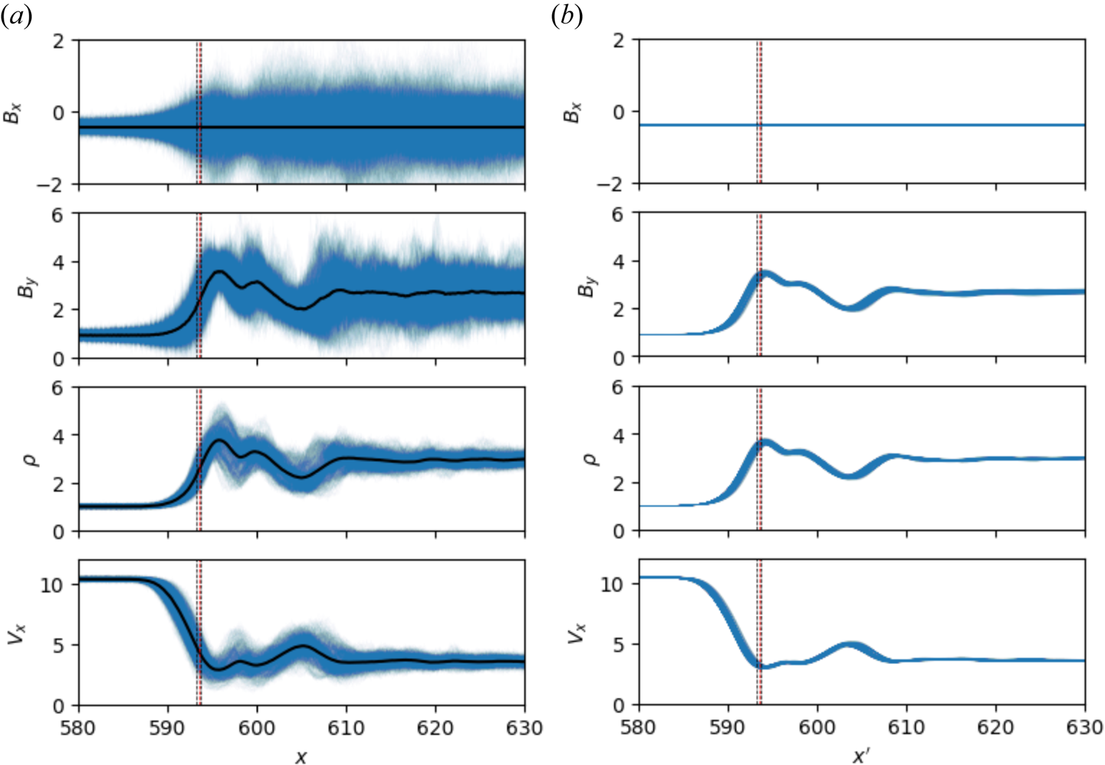
The basic properties of the shock are summarized in figure 8, which shows $x$ -profiles of the magnetic field components $B_x(x',y=\text {const}, t\varOmega _u=125)/B_u$
 , $B_y(x',y=\text {const}, t\varOmega _u=125)/B_u$
 , normal component of the velocity $V_x'(x',y=\text {const}, t\varOmega _u=125)/V_u$
 and density $\rho (x',y=\text {const}, t\varOmega _u=125)/\rho _u$
 , taken at various values of $y=\text {const}$
 (left column). Here, $V_x'=V_x+V_{sh}$
 is the velocity in NIF. There is substantial variance of the above variables. The right column shows the $y$
 -averaged profiles

where $X=B_x,B_y,V_x,\rho$ , for various moments in the time interval $125< t\varOmega _u <220$
 , and $x' = x + V_u(t-t_0)$
 is the NIF coordinate. The $y$
 -average profiles are stationary in NIF.
Profiles of (top to bottom) $B_x$ , $B_y$
 , $\rho$
 and $V_x$
 in the hybrid simulation. The left column shows $y=\text {const}$
 cuts taken at each cell, i.e. there are 2048 cuts, and a single instance of time $t\varOmega _{u}=125$
 . In each panel, each blue line is the single profile, e.g. $B_y(x, y=const, t=\text {const})$
 , while the black line corresponds to the $y$
 -average. The vertical dash lines mark the region used in the analysis of shock front perturbations and distribution function below. The right column shows $\langle B_x\rangle _y(x',t)$
 , $\langle B_y\rangle _y(x',t)$
 , $\langle V_x'\rangle _y(x',t)$
 and $\langle \rho \rangle _y(x',t)$
 , for various moments in the time interval $125< t\varOmega _u <220$
 . Here, $x' = x + V_u(t-t_0)$
 is the NIF coordinate, with $t_0\varOmega _u = 125$
 , and $V_x=V_x'+V_{sh}$
 .
.
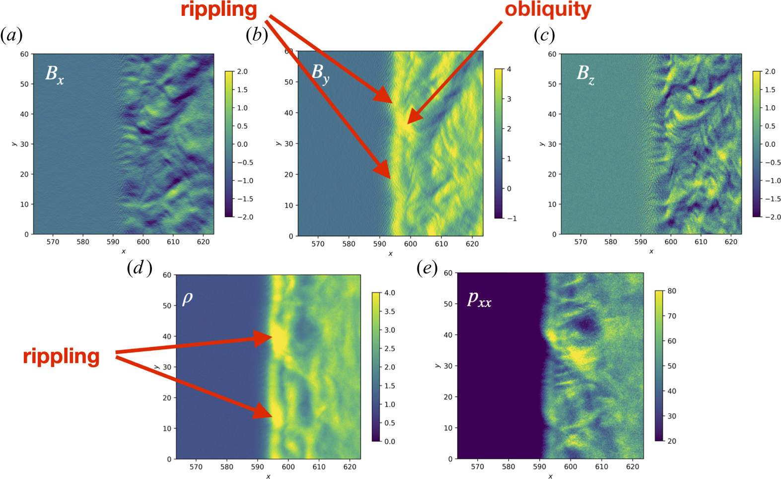
The structure of the shock front perturbations is further illustrated in figure 9, which shows a section of the simulation domain of size $(60 \times 60) c/\omega _{pi}$ near the shock front. Several distinct types of perturbations are present, with different wavelengths and polarization properties. We identify the shock rippling by the enhancements at the shock front, shown in the figure by red arrows. The wavelength of these fluctuations is approximately $25 c/\omega _{pi}$
 . These perturbations propagate in the negative $y$
 -direction, with the velocity $V_y \approx -6 V_A$
 . Note that the fronts of the rippling wave are not perpendicular to the shock front but are oblique. One of these fronts is along a red arrow in the figure. Figure 10 illustrates the frequency spectrum of $B_y$
 fluctuations along the shock front in the NIF. The spectrum is obtained by performing the fast Fourier transform of $B_y$
 collected in a narrow region around $x' = 593.5 c/\omega _{pi}$
 (see figure 8). The spectrum shows the existence of perturbations with wavenumbers in the range $k_y \lesssim 0.6$
 , propagating roughly with the same phase speed in the negative $y$
 direction. Further, there appears to exist a second class of weaker fluctuations, propagating in the opposite direction with a somewhat smaller phase speed.
Two-dimensional profiles of (clockwise) $B_x$ , $B_y$
 , $B_z$
 , $\rho$
 and pressure tensor $\hat p_{xx}$
 in a hybrid simulation at $t\varOmega _u=125$
 .
.
Frequency–wavenumber spectrum of $B_y$ fluctuations along the shock front.

The reduced ion distribution function collected in the same narrow region of $x$ is shown in figure 11. The same rippling as in figure 9 is seen in the reduced distribution function and is marked by red arrows. The rippling seems to be closely related to the non-locality of the reflection process is also seen (Gedalin Reference Gedalin2023).
Reduced distribution function at the shock front (left to right): $f(y,v_x)$ , $f(y,v_y)$
 , $f(y,v_z)$
 . The rightmost panel shows $B_y(y)$
 at the same $x$
 -location. The distributions are shown in the NIF.

Despite the spatial and time variability of the shock structure, the shock maintains stable average fluxes of the conserved quantities, as expected. This is shown in figure 12, which shows fluxes of mass $F_m$ , total momentum $F_p$
 and total energy $F_\epsilon$
 in the simulation, normalized to their corresponding upstream values. Omitting resistivity terms, the conserved fluxes take the following form in the hybrid model:


where

is the ion kinetic pressure tensor in the co-moving frame, and

is the ion heat flux. The fluxes in (3.10)–(3.12) are further $y$ -averaged. We observe that time-averaged fluxes of mass and momentum are conserved to approximately 0.5 % or better between the upstream and downstream regions. The average energy flux shows somewhat greater variation, a little over 1 %, across the region included in figure 12. This is likely due to a combination of numerical dissipation in the simulation and slight time variability of the upstream conditions (which could be traced to numerical dissipation in the upstream region).
Fluxes of (top to bottom) mass, momentum and energy in the hybrid simulation. In each panel, the coloured lines show flux computed at an instance of time as indicated by the colour bar. The black lines show time-averaged fluxes. Each flux is normalized by its upstream value.

3.4. A rippled shock: modelling
We model a rippled shock front assuming that the shock is approximately stationary in the frame moving with the ripples along the shock front with the ripple velocity $V_u(V_{ry},V_{rz})$ . We assume that the residual time dependence seen in the simulations is of secondary importance and may be ignored when modelling the shock structure. In what follows we exploit the principles proposed by Gedalin & Ganushkina (Reference Gedalin and Ganushkina2022). In the rippling frame, the upstream plasma velocity is $V_u(1,- V_{ry},-V_{rz})$
 , so that the electric field would be


if the shock were planar, which is denoted by the superscript ${(0)}$ . We introduce the scalar and vector potentials


where $\boldsymbol {B}^{(0)}$ is given by (3.1)–(3.3). Rippling is added by replacing the dependence on $x$
 with the dependence on


The shape (3.22) is a generalization of waveform proposed by Gedalin & Ganushkina (Reference Gedalin and Ganushkina2022) and is inspired by the above simulation showing that the front of the wave is not perpendicular to the shock front. Thus, rippling is a nonlinear wave propagating at an angle to the shock front. This wave damps into the downstream region and seems to not propagate into the upstream region. This behaviour is modelled using the localization function $g$ . The replacement $x\rightarrow X$
 is to be done in the vector potential and scalar potential. Then


where $B_z^{(0)}=B_z^{(0)}(X)$ , $B_y^{(0)}=B_y^{(0)}(X)$
 and $\psi _\xi =\partial \psi /\partial \xi$
 . For the present analysis, we add rippling to the non-structured shock profile (3.1). The parameters chosen to make the model resemble the simulated shock are


The three components of the magnetic of the rippled shock model are shown in figure 13 (central part only). Figure 14 further illustrates the structure of the magnetic field of the model, showing two families of the magnetic field magnitude cuts. The model was used to trace 160 000 ions. The incident distribution was the same Maxwellian as above. The initial $x$ and $y$
 were the same for all ions, while the initial $z$
 were randomly distributed along the wavelength $0\leq z<3$
 . Figure 15 presents the results of the tracing as a 2-D distribution of the ion pressure $p_{i,xx}$
 , where

The distribution function $f(\boldsymbol {v},x,z)$ is obtained by counting particles appearing in $500\times 50$
 cells of the size $\Delta x=0.018$
 and $\Delta y=0.06$
 . During the tracing $z$
 -coordinate of an ion may leave the stripe $0\leq z<3$
 . In this case, it is counted with $z$
 -coordinate shifted toward the stripe by adding an integer number of wavelengths. Each ion count is multiplied with the weight $|v_{0x}|$
 (Gedalin, Pogorelov & Roytershteyn Reference Gedalin, Pogorelov and Roytershteyn2023b). Figure 16 shows the reduced distribution function $f(x,v_x)=\int f(\boldsymbol {v},x,z) \,{\rm d} v_y\,{\rm d} v_z\,{\rm d} z$
 .
.
The three components of the magnetic of the rippled shock model. Three wavelengths along the shock front are shown.

(a) Value of $|B|/B_u$ as a function of $x$
 for various $z$
 . (b) Value of $|B|/B_u$
 as a function of $z$
 for various $x$
 .
.

(a) Value of $p_{i,xx}$ as a function of $x$
 and $z$
 . (b) Value of $B_x$
 as a function of $x$
 and $z$
 .
.

The reduced distribution function $f(x,v_x)$ .
.

The behaviour of ions is further illustrated by the cuts at $x=0$ . Figure 17 shows the distribution function $f(z,v_x)$
 at $x=0$
 . Figure 18 shows $z$
 -integrated distributions $f(v_x,v_y)$
 and $f(v_x,v_z)$
 for $x=0$
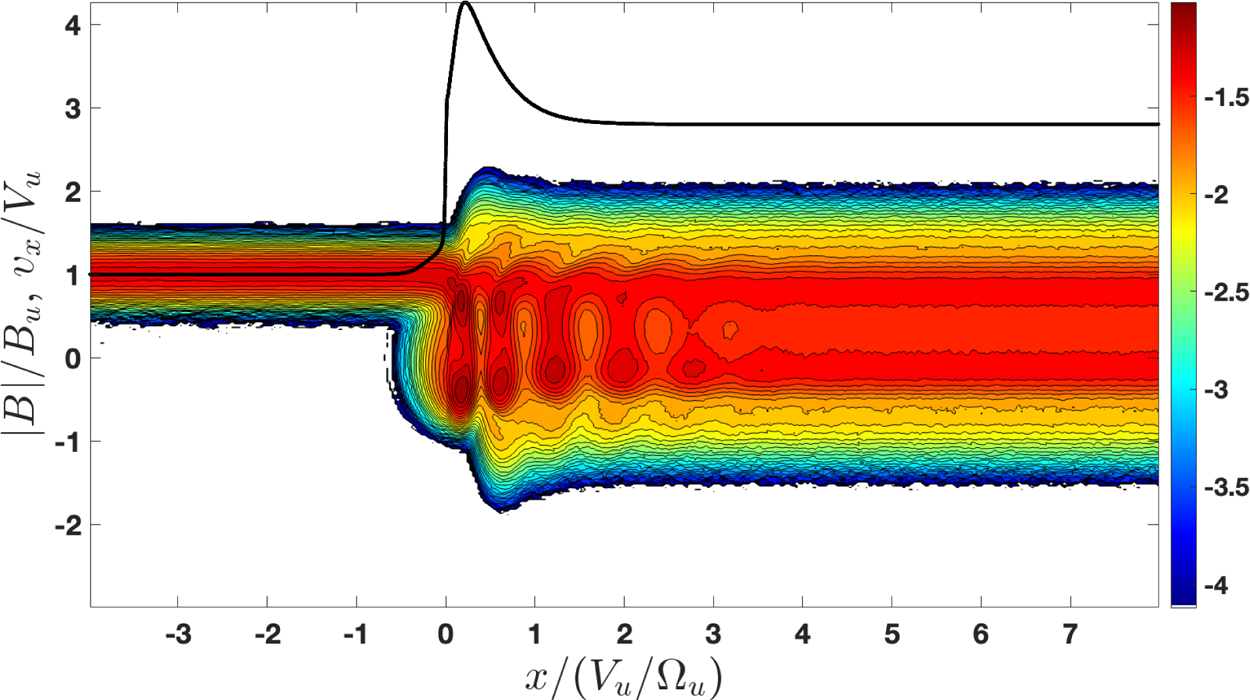
 . Finally, figure 19 shows the magnetic field magnitude calculated using the planar stationary momentum balance (3.6). Only the values far upstream and downstream have physical sense since in the region, where rippling is still noticeable, (3.6) is not valid and should be replaced with a more complicated version (Gedalin & Ganushkina Reference Gedalin and Ganushkina2022). The downstream value of $|B|/B_u$
 is rather close to $B_d/B_u$
 chosen in the model.
The distribution function $f(z,v_x)$ at $x=0$
 .
.

(a) Value of $f(v_x,v_y)$ at $x=0$
 . (b) Value of $f(v_x,v_z)$
 at $x=0$
 .
.

The magnetic field magnitude calculated using the planar stationary momentum balance (3.6). The derived downstream magnetic field is consistent with the chosen model magnetic field. The conversion to the downstream value starts rather quickly, less than three ion upstream convective gyroradii.

4. Discussion and conclusions
To remind a reader, the main objective of the present study was to analyse whether parameters similar to those of the observed shock crossing are consistent with a planar stationary shock profile, either non-structured or structured or non-planarity, and time dependence, e.g. in the form of ripples propagating along the shock front, are required to maintain the conservation laws. Starting with the upstream shock parameters, namely, the Alfvénic Mach number, shock angle and upstream temperature, we have shown that the magnetic compression, predicted by the Rankine–Hugoniot relations, cannot be achieved in a planar stationary shock without breaking the momentum conservation (3.6) throughout the shock. Using hybrid simulations, we found that the shock with parameters similar to those of the observed shock is rippled. In the NIF, this rippling is a large-amplitude nearly monochromatic wave propagating with a constant speed along the shock front. The amplitude of the ripples is the largest in the vicinity of the ramp and overshoot, sharply dropping toward upstream and slowly decaying in the downstream region. In the frame moving with the speed of ripples along the shock front, the overall pattern of shock transition layer and the downstream region is spatially non-uniform but nearly time-independent. In NIF, where the ripples are moving, the pattern is significantly time-dependent. Observations (Johlander et al. Reference Johlander, Schwartz, Vaivads, Khotyaintsev, Gingell, Peng, Markidis, Lindqvist, Ergun and Marklund2016; Gingell et al. Reference Gingell, Schwartz, Burgess, Johlander, Russell, Burch, Ergun, Fuselier, Gershman and Giles2017; Johlander et al. Reference Johlander, Vaivads, Khotyaintsev, Gingell, Schwartz, Giles, Torbert and Russell2018) support the numerically established picture of ripples propagating in NIF. It is not known at present whether ripples can stand in NIF. The mass, momentum and energy fluxes significantly vary in space and time but the averaged fluxes are constant throughout the shock. The 2-D simulation allowed us to determine the plausible rippling parameters which were further used for modelling the rippled shock and test particle analysis of the ion motion in this model. The far downstream magnetic field, derived from ion tracing in the model, is consistent with the magnetic field chosen in the model. We interpret the results of the study as an indication of a ‘phase transition’ from a planar stationary regime to a rippled regime, in a way similar to the transition from an almost monotonic profile in subcritical shocks to a well-structured profile in supercritical shocks. Such a ‘phase transition’ should occur simply because of the necessity to maintain stable fluxes of mass, momentum and energy, and would occur whatever is a specific mechanism of rippling onset. At present, we do not know what are thresholds in the parameter range required to be crossed for such a transition.
Acknowledgements
This work was partially supported by the International Space Science Institute (ISSI) in Bern, through International Team project #23-575. V.R. was partially supported by NASA grant 80NSSC21K1680 and by NSF grant 2010144. Computational resources were provided by the NASA High-End Computing (HEC) Program through the NASA Advanced Supercomputing (NAS) Division at Ames Research Center.
Editor Luís O. Silva thanks the referees for their advice in evaluating this article.
Declaration of interests
The authors report no conflict of interest.


 Open access