

I. INTRODUCTION
A major research pursuit in the area of signal processing on graphs [Reference Shuman, Narang, Frossard, Ortega and Vandergheynst1,Reference Sandryhaila and Moura2] has been to design multiscale wavelet and vertex-frequency transforms [Reference Crovella and Kolaczyk3–Reference Shuman, Faraji and Vandergheynst24]. Objectives of these transforms are to sparsely represent different classes of graph signals and/or efficiently reveal relevant structural properties of high-dimensional data on graphs. As we move forward, it is important to test both of these transforms on myriad applications, as well as to develop additional theory to help answer the question of which transforms are best suited to which types of data.
Uncertainty principles such as the ones presented in [Reference Matolcsi and Szücs25–Reference Ricaud and Torrésani32] are an important tool in designing and evaluating linear transforms for processing “classical” signals such as audio signals, time series, and images residing on Euclidean domains. It is desirable that the dictionary atoms are jointly localized in time and frequency, and uncertainty principles characterize the resolution tradeoff between these two domains. Moreover, while “the uncertainty principle is [often] used to show that certain things are impossible”, Donoho and Stark [Reference Donoho and Stark26] present “examples where the generalized uncertainty principle shows something unexpected is possible; specifically, the recovery of a signal or image despite significant amounts of missing information”. In particular, uncertainty principles can provide guarantees that if a signal has a sparse decomposition in a dictionary of incoherent atoms, this is indeed a unique representation that can be recovered via optimization [Reference Donoho and Huo27,Reference Elad and Bruckstein28]. This idea underlies the recent wave of sparse signal processing techniques, with applications such as denoising, source separation, inpainting, and compressive sensing. While there is still limited theory showing that different mathematical classes of graph signals are sparsely represented by the recently proposed transforms (see [Reference Ricaud, Shuman and Vandergheynst33] for one preliminary work along these lines), there is far more empirical work showing the potential of these transforms to sparsely represent graph signals in various applications.
Many of the multiscale transforms designed for graph signals attempt to leverage intuition from signal processing techniques designed for signals on Euclidean data domains by generalizing fundamental operators and transforms to the graph setting (e.g., by checking that they correspond on a ring graph). While some intuition, such as the notion of filtering with a Fourier basis of functions that oscillate at different rates (see, e.g., [Reference Shuman, Narang, Frossard, Ortega and Vandergheynst1]) carries over to the graph setting, the irregular structure of the graph domain often restricts our ability to generalize ideas. One prime example is the lack of a shift-invariant notion of translation of a graph signal. As shown in [Reference McGraw and Menzinger34,Reference Saito and Woei35] and discussed in [Reference Shuman, Ricaud and Vandergheynst23, Section 3.2], the concentration of the Fourier basis functions is another example where the intuition does not carry over directly. Complex exponentials, the basis functions for the classical Fourier transform, have global support across the real line. On the other hand, the eigenvectors of the combinatorial or normalized graph Laplacians, which are most commonly used as the basis functions for a graph Fourier transform, are sometimes localized to small regions of the graph. Because the incoherence between the Fourier basis functions and the standard normal basis underlies many uncertainty principles, we demonstrate this issue with a short example.
Motivating Example (Part I: Laplacian eigenvector localization)
Let us consider the two manifolds (surfaces) embedded in  ${\open R^3}$ and shown in the first row of Fig. 1. The first one is a flat square. The second is identical except for the center where it contains a spike. We sample both of these manifolds uniformly across the x-y plane and create a graph by connecting the 8 nearest neighbors with weights depending on the distance (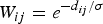 $W_{ij}=e^{-d_{ij}/\sigma}$). The energy of each Laplacian eigenvector of the graph arising from the first manifold is not concentrated on any particular vertex; i.e.,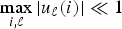 $\max_{i\comma \ell}\vert u_{\ell}\lpar i\rpar \vert \ll 1$, where uℓ is the eigenvector associated with eigenvalue $\lambda_{\ell}$. However, the graph arising from the second manifold does have a few eigenvectors, such as eigenvector 3 shown in the middle row Fig. 1, whose energy is highly concentrated on the region of the spike; i.e: $\max_{i\comma \ell}\vert u_{\ell}\lpar i\rpar \vert \approx 1$. Yet, the Laplacian eigenvectors of this second graph whose energy resides primarily on the flatter regions of the manifold, such as eigenvector 17 shown in the bottom row of Fig. 1, are not too concentrated on any single vertex. Rather, they more closely resemble some of the Laplacian eigenvectors of the graph arising from the first manifold.
Concentration of graph Laplacian eigenvectors. We discretize two different manifolds by sampling uniformly across the x-y plane. Due to its bumpy central part, the graph arising from manifold 2 has a graph Laplacian eigenvector (shown in the middle row of the right column) that is highly concentrated in both the vertex and graph spectral domains. However, the eigenvectors of this graph whose energy primarily resides in the flatter parts of the manifold (such as the one shown in the bottom row of the right column) are less concentrated, and some closely resemble the Laplacian eigenvectors of the graph arising from the flat manifold 1 (such as the corresponding eigenvector shown in the bottom row of the left column.

Below we discuss three different families of uncertainty principles, and their extensions to the graph setting, both in prior work and in this contribution.
• The first family of uncertainty principles measure the spreading around some reference point, usually the mean position of the energy contained in the signal. The well-known Heisenberg uncertainty principle [Reference Folland and Sitaram36,Reference Mallat37] belongs to this family. It views the modulus square of the signal in both the time and Fourier domains as energy probability density functions, and takes the variance of those energy distributions as measures of the spreading in each domain. The uncertainty principle states that the product of variances in the time and in the Fourier domains cannot be arbitrarily small. The generalization of this uncertainty principle to the graph setting is complex since there does not exist a simple formula for the mean value or the variance of graph signals, in either the vertex or the graph spectral domains. For unweighted graphs, Agaskar and Lu [Reference Agaskar and Lu38–Reference Agaskar and Lu40] also view the square modulus of the signal in the vertex domain as an energy probability density function and use the geodesic graph distance (shortest number of hops) to define the spread of a graph signal around a given center vertex. For the spread of a signal f in the graph spectral domain, Agaskar and Lu use the normalized variation $\lpar {f^{\top}{\cal L} f}\rpar /{\Vert f\Vert _{2}^{2}}$, which captures the smoothness of a signal. They then specify uncertainty curves that characterize the tradeoff between the smoothness of a graph signal and its localization in the vertex domain. This idea is generalized to weighted graphs in [Reference Pasdeloup, Alami, Gripon and Rabbat41]. As pointed out in [Reference Agaskar and Lu40], the tradeoff between smoothness and localization in the vertex domain is intuitive as a signal that is smooth with respect to the graph topology cannot feature values that decay too quickly from the peak value. However, as shown in Fig. 1 (and subsequent examples in Table 1), graph signals can indeed be simultaneously highly localized or concentrated in both the vertex domain and the graph spectral domain. This discrepancy is because the normalized variation used as the spectral spread in [Reference Agaskar and Lu40] is one method to measure the spread of the spectral representation around the eigenvalue 0, rather than around some mean of that signal in the graph spectral domain. In fact, using the notion of spectral spread presented in [Reference Agaskar and Lu40], the graph signal with the highest spectral spread on a graph ${\cal G}$ is the graph Laplacian eigenvector associated with the highest eigenvalue. The graph spectral representation of that signal is a Kronecker delta whose energy is completely localized at a single eigenvalue. One might argue that its spread should in fact be zero. So, in summary, while there does exist a tradeoff between the smoothness of a graph signal and its localization around any given center vertex in the vertex domain, the classical idea that a signal cannot be simultaneously localized in the time and frequency domains does not always carry over to the graph setting. While certainly an interesting avenue for continued investigation, we do not discuss uncertainty principles based on spreads in the vertex and graph spectral domains any further in this paper.
• The second family of uncertainty principles involve the absolute sparsity or concentration of a signal. The key quantities are typically either support measures counting the number of non-zero elements, or concentration measures, such as ℓp-norms. An important distinction is that these sparsity and concentration measures are not localization measures. They can give the same values for different signals, independent of whether the predominant signal components are clustered in a small region of the vertex domain or spread across different regions of the graph. An example of a recent work from the graph signal processing literature that falls into this family is [Reference Tsitsvero, Barbarossa and Di Lorenzo42], in which Tsitsvero et al. propose an uncertainty principle that characterizes how jointly concentrated graph signals can be in the vertex and spectral domains. Generalizing prolate spheroidal wave functions [Reference Slepian and Pollak43], their notion of concentration is based on the percentage of energy of a graph signal that is concentrated on a given set of vertices in the vertex domain and a given set of frequencies in the graph spectral domain. Another example of graph uncertainty principle is presented in Theorems 5.1 and 5.2 of [Reference Pesenson44]. It is a trade-off between the Poincare constant ΛS that measures the size (capacity) of a set S and the bandlimit frequency w of the functions living on that space.
Since we can interpret signals defined on graphs as finite-dimensional vectors with well-defined ℓp-norms, we can also apply directly the results of existing uncertainty principles for finite dimensional signals. As one example, the Elad–Bruckstein uncertainty principle of [Reference Elad and Bruckstein28] states that if α and β are the coefficients of a vector
$f \in {\open R}^{N}$ in two different orthonormal bases, then
(1)where μ is the maximum magnitude of the inner product between any vector in the first basis with any vector in the second basis. In Section III-A, we apply (1) to graph signals by taking one basis to be the canonical basis of Kronecker delta functions in the graph vertex domain and the other to be a Fourier basis of graph Laplacian eigenvectors. We also apply other such finite dimensional uncertainty principles from [Reference Ricaud and Torrésani32,Reference Folland and Sitaram36,Reference Maassen and Uffink45] to the graph setting. In Section III-B, we adapt the Hausdorff–Young inequality [Reference Reed and Simon46, Section IX.4], a classical result for infinite dimensional signals, to the graph setting. These results typically depend on the mutual coherence between the graph Laplacian eigenvectors and the canonical basis of deltas. For the special case of shift-invariant graphs with circulant graph Laplacians [Reference Grady and Polimeni47, Section 5.1], such as ring graphs, these bases are incoherent, and we can attain meaningful uncertainty bounds. However, for less homogeneous graphs (e.g., a graph with a vertex with a much higher or lower degree than other vertices), the two bases can be more coherent, leading to weaker bounds. Moreover, as we discuss in Section II, the bounds are global bounds, so even if the majority of a graph is for example very homogenous, inhomogeneity in one small area can prevent the result from informing the behavior of graph signals across the rest of the graph.$${\Vert\alpha\Vert_0 + \Vert\beta\Vert_0 \over 2} \geq \sqrt{\Vert\alpha\Vert_0 \cdot \Vert\beta\Vert_0} \geq {1 \over \mu}\comma$$• The third family of uncertainty principles characterize a single joint representation of time and frequency. The short-time Fourier transform (STFT) is an example of a time-frequency representation that projects a function f onto a set of translated and modulated copies of a function g. Usually, g is a function localized in the time-frequency plane, for example a Gaussian, vanishing away from some known reference point in the joint time and frequency domain. Hence this transformation reveals local properties in time and frequency of f by separating the time–frequency domain into regions where the translated and modulated copies of g are localized. This representation obeys an uncertainty principle: the STFT coefficients cannot be arbitrarily concentrated. This can be shown by estimating the different ℓp-norms of this representation (note that the concentration measures of the second family of uncertainty principles are used). For example, Lieb [Reference Lieb48] proves a concentration bound on the ambiguity function (e.g., the STFT coefficients of the STFT atoms). Lieb's approach is more general than the Heisenberg uncertainty principle, because it handles the case where the signal is concentrated around multiple different points (see, e.g., the signal f 3 in Fig. 2).
In Section V, we generalize Lieb's uncertainty principle to the graph setting to provide upper bounds on the concentration of the transform coefficients of any graph signal under (i) any frame of dictionary atoms, and (ii) a special class of dictionaries called localized spectral graph filter frames, whose atoms are of the form T i g k, where T i is a localization operator that centers on vertex i a pattern described in the graph spectral domain by the kernel
$\widehat{g_{k}}$.
Fig. 2.The concentration s p(·) of four different example signals (all with 2-norm equal to 1), for various values of p.Note that the position of the signal coefficients does not matter for this concentration measure. Different values of p lead to different notions of concentration; for example, f 2 is more concentrated than f 3 if p = ∞ (it has a larger maximum absolute value), but less concentrated if p = 1.
Table 1.Numerical values of the uncertainty bound maxi,k∥T ig k∥2 of Example 5 for various graphs of 64 nodes.



While the second family of uncertainty principles above yields global uncertainty principles, we can generalize the third family to the graph setting in a way that yields local uncertainty principles. In the classical Euclidean setting, the underlying domain is homogenous, and thus uncertainty principles apply to all signals equally, regardless of where on the real line they are concentrated. However, in the graph setting, the underlying domain is irregular, and a change in the graph structure in a single small region of the graph can drastically affect the uncertainty bounds. For instance, the second family of uncertainty principles all depend on the coherence between the graph Laplacian eigenvectors and the standard normal basis of Kronecker deltas, which is a global quantity in the sense that it incorporates local behavior from all regions of the graph. To see how this can limit the usefulness of such global uncertainty principles, we return to the motivating example from above.
Motivating Example (Part II: Global versus local uncertainty principles)
In Section III-A, we show that a direct application of a result from [Reference Ricaud and Torrésani32] to the graph setting yields the following uncertainty relationship, which falls into the second family described above, for any signal  $f \in {\open R}^{N}$:
 $$\left({\Vert f \Vert_2 \over \Vert f \Vert_1}\right)\left({\Vert \hat{f} \Vert_2 \over \Vert \hat{f} \Vert_1}\right)\leq {\max_{i\comma \ell}\vert u_\ell\lpar i\rpar \vert }.$$
Each fraction in the left-hand side of (2) is a measure of concentration that lies in the interval  $\lsqb \lpar {1}/{\sqrt{N}\rpar }\comma \; 1\rsqb $ (N is the number of vertices), and the coherence between the graph Laplacian eigenvectors and the Kronecker deltas on the right-hand side lies in the same interval. On the graph arising from manifold 1, the coherence is close to ${1}/{\sqrt{N}}$, and (2) yields a meaningful uncertainty principle. However, on the graph arising from manifold 2, the coherence is close to 1 due to the localized eigenvector 3 in Fig. 1. In this case, (2) is trivially true for any signal in ${\open R}^{N}$ from the properties of vector norms, and thus the uncertainty principle is not particularly useful. Nevertheless, far away from the spike, signals should behave similarly on manifold 2 to how they behave on manifold 1. Part of the issue here is that the uncertainty relationship holds for any graph signal f, even those concentrated on the spike, which we know can be jointly localized in both the vertex and graph spectral domains. An alternative approach is to develop a local uncertainty principle that characterizes the uncertainty in different regions of the graph on a separate basis. Then, if the energy of a given signal is concentrated on a more homogeneous part of the graph, the concentration bounds will be tighter.
In Section VI, we generalize the approach of Lieb to build a local uncertainty principle that bounds the concentration of the analysis coefficients of each atom of a localized graph spectral filter frame in terms of quantities that depend on the local structure of the graph around the center vertex of the given atom. Thus, atoms localized to different regions of the graph feature different concentration bounds. Such local uncertainty principles also have constructive applications, and we conclude with an example of non-uniform sampling for graph inpainting, where the varying uncertainty levels across the graph suggest a strategy of sampling more densely in areas of higher uncertainty. For example, if we were to take M measurements of a smooth signal on manifold 2 in Fig. 1, this method would lead to a higher probability of sampling signal values near the spike, and a lower probability of sampling signal values in the more homogenous flat parts of the manifold, where reconstruction of the missing signal values is inherently easier.
II. NOTATION AND GRAPH SIGNAL CONCENTRATION
In this section, we introduce some notation and illustrate further how certain intuition from signal processing on Euclidean spaces does not carry over to the graph setting.
A) Notation
Throughout the paper, we consider signals residing on an undirected, connected, and weighted graph  ${\cal G} = \lcub {\cal V}\comma \; {\cal E}\comma \; {\bf W\rcub }$, where ${\cal V}$ is a finite set of N vertices ( $\vert {\cal V}\vert = N$), ${\cal E}$ is a finite set of edges, and W is the weight or adjacency matrix. The entry W ij of W represents the weight of an edge connecting vertices i and j. We denote the complement of a set S by S c. A graph signal $f\colon {\cal V} \rightarrow {\open C}$ is a function assigning one value to each vertex. Such a signal f can be written as a vector of size N with the n th component representing the signal value at the n th vertex. The generalization of Fourier analysis to the graph setting requires a graph Fourier basis $\lcub u_{\ell}\rcub _{\ell \in \lcub 0\comma 1\comma \ldots\comma N-1\rcub }$. The most commonly used graph Fourier bases are the eigenvectors of the combinatorial (or non-normalized) graph Laplacian, which is defined as ${\cal L} = {\bf D} - {\bf W}$, where D is the diagonal degree matrix with diagonal entries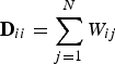 ${\bf D}_{ii}=\sum_{j=1}^{N} W_{ij}$, and $i \in {\cal V}$, or the eigenvectors of the normalized graph Laplacian $\tilde{\cal L}={\bf D}^{-\lpar {1}/{2}\rpar } {\cal L} {\bf D}^{-\lpar {1}/{2}\rpar }$. However, the eigenbases (or Jordan eigenbases) of other matrices such as the adjacency matrix have also been used as graph Fourier bases [Reference Sandryhaila and Moura2,Reference Sandryhaila and Moura49]. All of our results in this paper hold for any choice of the graph Fourier basis. For concreteness, we use the combinatorial Laplacian, which has a complete set of orthonormal eigenvectors $\lcub u_{l}\rcub _{l \in \lcub 0\comma 1\comma \ldots\comma N-1\rcub }$ associated with the real eigenvalues $0=\lambda_{0} \lt \lambda_{1} \leq \lambda_{2} \leq \cdots \leq \lambda_{N-1} = \lambda_{\rm max}$. We denote the entire Laplacian spectrum by $\sigma\lpar \L\rpar =\lcub \lambda_{0}\comma \; \ldots\comma \; \lambda_{N-1}\rcub $. The graph Fourier transform $\hat{f}\in {\open C}^{N}$ of a function $f \in {\open C}^{N}$ defined on a graph $\cal G$ is the projection of the signal onto the orthonormal graph Fourier basis $\lcub u_{\ell}\rcub _{\ell=0\comma 1\comma \ldots\comma N-1}$, which we take to be the eigenvectors of the graph Laplacian associated with ${\cal G}$:
 $$\eqalign{ &\hat{f}\lpar \lambda_\ell\rpar =\langle f\comma \; u_{\ell} \rangle= \sum_{n=1}^N f\lpar n\rpar \overline{u_{\ell}\lpar n\rpar }\comma \; \cr & \quad \quad \ell \in \lcub 0\comma \; 1\comma \; \ldots\comma \; N-1\rcub .}$$
See, for example, [Reference Chung50] for more details on spectral graph theory, and [Reference Shuman, Narang, Frossard, Ortega and Vandergheynst1] for more details on signal processing on graphs.
B) Concentration measures
In order to discuss uncertainty principles, we must first introduce some concentration/sparsity measures. Throughout the paper, we use the terms sparsity and concentration somewhat interchangeably, but we reserve the term spread to describe the spread of a function around some mean or center point, as discussed in the first family of uncertainty principles in Section I. The first concentration measure is the support measure of f, denoted ‖f‖0, which counts the number of non-zero elements of f. The second concentration measure is the Shannon entropy, which is used often in information theory and physics:
 $$H\lpar f\rpar =-\displaystyle\sum_{n} \vert f\lpar n\rpar \vert ^2\ln\vert f\lpar n\rpar \vert ^2\comma \;$$
where the variable n has values in {1,2,…,N} for functions on graphs and  $\lcub 0\comma \; 1\comma \; \ldots\comma \; N-1\rcub $ in the graph Fourier representation. Another class of concentration measures is the ℓp-norms, with $p\in\lsqb 1\comma \; \infty\rsqb $. For p ≠ 2, the sparsity of f may be measured using the following quantity:
 $$s_p\lpar f\rpar = \left\{\matrix{\displaystyle{\Vert f\Vert_2 \over \Vert f\Vert_p}\comma \; &\hbox{if } 1 \leq p \leq 2 \cr \displaystyle{\Vert f\Vert_p \over \Vert f\Vert_2}\comma \; &\hbox{if } 2 \lt p \leq \infty }\right..$$
For any vector  $f \in {\open C}^{N}$ and any $p \in \lsqb 1\comma \; \infty\rsqb $, $s_{p}\lpar f\rpar \in \lsqb N^{-\vert \lpar {1}/{p}\rpar -\lpar {1}/{2}\rpar \vert }\comma \; 1\rsqb $. If s p(f) is high (close to 1), then f is sparse, and if s p(f) is low, then f is not concentrated. Figure 2 uses some basic signals to illustrate this notion of concentration, for different values of p. In addition to sparsity, one can also relate ℓp-norms to the Shannon entropy via Renyi entropies (see, e.g., [Reference Rényi51,Reference Ricaud and Torrésani52] for more details).
C) Concentration of the graph Laplacian eigenvectors
The spectrum of the graph Laplacian replaces the frequencies as coordinates in the Fourier domain. For the special case of shift-invariant graphs with circulant graph Laplacians [Reference Grady and Polimeni47, Section 5.1], the Fourier eigenvectors can still be viewed as pure oscillations. However, for more general graphs (i.e., all but the most highly structured), the oscillatory behavior of the Fourier eigenvectors must be interpreted more broadly. For example, [1, Fig. 3] displays the number of zero crossings of each eigenvector; that is, for each eigenvector, the number of pairs of connected vertices where the signs of the values of the eigenvector at the connected vertices are opposite. It is generally the case that the graph Laplacian eigenvectors associated with larger eigenvalues contain more zero crossings, yielding a notion of frequency to the graph Laplacian eigenvalues. However, despite this broader notion of frequency, the graph Laplacian eigenvectors are not always globally-supported, pure oscillations like the complex exponentials. In particular, they can feature sharp peaks, meaning that some of the Fourier basis elements can be much more similar to an element of the canonical basis of Kronecker deltas on the vertices of the graph. As we will see, uncertainty principles for signals on graphs are highly affected by this phenomenon.
Coherence between the graph Fourier basis and the canonical basis for the graphs described in Example 1. Top left: Comet graphs with k = 6 and k = 12 branches, all of length one except for one of length ten. Top right: Evolution of the graph Fourier coherence  $\mu_{\cal G}$ with respect to k. Bottom left: Example of a modified path graph with 10 nodes. Bottom right: Evolution of the coherence of the modified path graph with respect to the distance between nodes 1 and 2. As the degree of the comet's center vertex increases or the first node of the modified path is pulled away, the coherence $\mu_{\cal G}$ tends to the limit value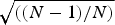 $\sqrt{\lpar \lpar {N-1}\rpar /{N}\rpar }$.

One way to compare a graph Fourier basis to the canonical basis is to compute the coherence between these two representations.
Definition 1 (Graph Fourier Coherence $\mu_{\cal G}$)

Let  ${\cal G}$ be a graph of N vertices. Let $\lcub \delta_{i}\rcub _{i\in \lcub 1\comma 2\comma \ldots\comma N\rcub }$ denote the canonical basis of $\ell^{2}\lpar {\open C}^{N}\rpar $ of Kronecker deltas and let $\lcub u_{\ell}\rcub _{\ell\in \lcub 0\comma 1\comma \ldots\comma N-1\rcub }$ be the orthonormal basis of eigenvectors of the graph Laplacian of ${\cal G}$. The graph Fourier coherence is defined as:
 $$\mu_{\cal G}=\mathop {\max }\limits_{i\comma \ell }\vert \langle \delta_i\comma \; u_{\ell}\rangle\vert =\mathop {\max }\limits_{i\comma \ell }\vert u_{\ell}\lpar i\rpar \vert =\mathop {\max }\limits_{\ell } s_{\infty}\lpar u_{\ell}\rpar .$$
 This quantity measures the similarity between the two sets of vectors. If the sets possess a common vector, then  $\mu_{\cal G}=1$ (the maximum possible value for $\mu_{\cal G}$). If the two sets are maximally incoherent, such as the canonical and Fourier bases in the standard discrete setting, then $\mu_{\cal G}=1/\sqrt{N}$ (the minimum possible value).
Because the graph Laplacian matrix encodes the weights of the edges of the graph, the coherence  $\mu_{\cal G}$ clearly depends on the structure of the underlying graph. It remains an open question exactly how structural properties of weighted graphs such as the regularity, clustering, modularity, and other spectral properties can be linked to the concentration of the graph Laplacian eigenvectors. For certain classes of random graphs [Reference Dekel, Lee and Linial53–Reference Tran, Vu and Wang55] or large regular graphs [Reference Brooks and Lindenstrauss56], the eigenvectors have been shown to be non-localized, globally oscillating functions (i.e., $\mu_{\cal G}$ is low). Yet, empirical studies such as [Reference McGraw and Menzinger34] show that graph Laplacian eigenvectors can be highly concentrated (i.e., $\mu_{\cal G}$ can be close to 1), particularly when the degree of a vertex is much higher or lower than the degrees of other vertices in the graph. The following example illustrates how $\mu_{\cal G}$ can be influenced by the graph structure.
Example 1
In this example, we discuss two classes of graphs that can have high graph Fourier coherences. The first, called comet graphs, are studied in [Reference Saito and Woei35,Reference Nakatsukasa, Saito and Woei57]. They are composed of a star with k vertices connected to a center vertex, and a single branch of length greater than one extending from one neighbor of the center vertex (see Fig. 3, top). If we fix the length of the longest branch (it has length 10 in Fig. 3), and increase k, the number of neighbors of the center vertex, the graph Laplacian eigenvector associated with the largest eigenvalue approaches a Kronecker delta centered at the center vertex of the star. As a consequence, the coherence between the graph Fourier and the canonical bases approaches 1 as k increases.
The second class are the modified path graphs, which we use several times in this contribution. We start with a standard path graph of 10 nodes equally spaced (all edge weights are equal to one) and we move the first node out to the left; i.e., we reduce the weight between the first two nodes (see Fig. 3, bottom). The weight is related to the distance by W12 = 1/d(1, 2) with d(1, 2) being the distance between nodes 1 and 2. When the weight between nodes 1 and 2 decreases, the eigenvector associated with the largest eigenvalue of the Laplacian becomes more concentrated, which increases the coherence  $\mu_{\cal G}$. These two examples of simple families of graphs illustrate that the topology of the graph can impact the graph Fourier coherence, and, in turn, uncertainty principles that depend on the coherence.
In Fig. 4, we display the eigenvector associated with the largest graph Laplacian eigenvalue for a modified path graph of 100 nodes, for several values of the weight W12. Observe that the shape of the eigenvector has a sharp local change at node 1.
Eigenvectors associated with the largest graph Laplacian eigenvalue of the modified path graph with 100 nodes, for different values of W 12. As the distance between the first two nodes increases, the eigenvector becomes sharply peaked.

Example 1 demonstrates an important point to keep in mind. A small local change in the graph structure can greatly affect the behavior of one eigenvector, and, in turn, a global quantity such as  $\mu_{\cal G}$. However, intuitively, a small local change in the graph should not drastically change the processing of signal values far away, for example in a denoising or inpainting task. For this reason, in Section VI, we introduce a notion of local uncertainty that depicts how the graph is behaving locally.
Note that not only special classes of graphs or pathological graphs yield highly localized graph Laplacian eigenvectors. Rather, graphs arising in applications such as sensor or transportation networks, or graphs constructed from sampled manifolds (such as the graph sampled from manifold 2 in Fig. 1) can also have graph Fourier coherences close to 1 (see, e.g., [Reference Shuman, Ricaud and Vandergheynst23, Section 3.2] for further examples).
III. GLOBAL UNCERTAINTY PRINCIPLES RELATING THE CONCENTRATION OF GRAPH SIGNALS IN TWO DOMAINS
In this section, we derive basic uncertainty principles using concentration measures and highlight the limitations of those uncertainty principles.
A) Direct applications of uncertainty principles for discrete signals
We start by applying five known uncertainty principles for discrete signals to the graph setting.
Theorem 1
Let  $f \in {\open C}^{N}$ be a non-zero signal defined on a connected, weighted, undirected graph ${\cal G}$, let $\lcub u_{\ell}\rcub _{\ell=0\comma 1\comma \ldots\comma N-1}$ be a graph Fourier basis for ${\cal G}$, and let $\mu_{\cal G}=\max_{i\comma \ell}\vert \langle\delta_{i}\comma \; u_{\ell}\rangle\vert $. We have the following five uncertainty principles:
(i) the support uncertainty principle [Reference Elad and Bruckstein28]
(4)$${{\Vert {f}\Vert}_0+{\Vert{\hat f}\Vert}_0 \over 2}\ge\sqrt{{\Vert {f}\Vert}_0{\Vert{\hat f}\Vert}_0}\ge{1 \over \mu_{\cal G}}.$$(ii) The ℓp-norm uncertainty principle [Reference Ricaud and Torrésani32]
(5)$$\Vert f\Vert _{p}\Vert {\hat f}\Vert _{p}\geq \mu_{\cal G}^{1-\lpar {2}/{p}\rpar }\Vert f\Vert _{2}^2 \comma \; \qquad p\in\lsqb 1\comma \; 2\rsqb .$$(iii) The entropic uncertainty principle [Reference Maassen and Uffink45]
(6)$$H\lpar f\rpar +H\lpar {\hat f}\rpar \ge -2\ln\mu_{\cal G}.$$(iv) The “local” uncertainty principle [Reference Folland and Sitaram36]
(7)$$\sum_{i\in {\cal V}_S}\vert f\lpar i\rpar \vert ^2\leq \vert {\cal V}_S\vert \Vert f\Vert _\infty^2 \le\vert {\cal V}_S\vert \mu_{\cal G}^2\Vert {\hat f}\Vert _1^2$$for any subset
${\cal V}_S$ of the vertices ${\cal V}$ in the graph ${\cal G}$.(v) The strong annihilating pair uncertainty principle [Reference Ghobber and Jaming31]
(8)$$\eqalign{ &\sqrt{\sum_{i \in {\cal V}_S^c} \vert f\lpar i\rpar \vert ^2 } + \sqrt{\sum_{\lambda_{\ell} \in \Lambda_T^c} \vert \hat{f}\lpar \lambda_{\ell}\rpar \vert ^2 } \cr &\quad\geq \left(1+{1 \over 1-\mu_{\cal G}\sqrt{\vert {\cal V}_S\vert \vert \Lambda_T\vert }}\right)^{-1} \Vert f\Vert _2\comma \; }$$for any subsets
$\cal V_S$ of the vertices $\cal V$ in the graph $\cal G$ and ΛT of the graph Laplacian spectrum σ($\cal L$) of $\cal G$ satisfying
$$\vert \cal V_S\vert \vert \Lambda_T\vert \lt \displaystyle{1 \over \mu_{\cal G}^2}.$$


The first uncertainty principle is given by a direct application of the Elad–Bruckstein inequality [Reference Elad and Bruckstein28]. It states that the sparsity of a function in one representation limits the sparsity in a second representation. As displayed in (1), the work of [Reference Elad and Bruckstein28] holds for representations in any two bases. As we have seen, if we focus on the canonical basis  $\lcub \delta_{i}\rcub _{i=1\comma \dots\comma N}$ and the graph Fourier basis $\lcub u_{\ell}\rcub _{\ell=0\comma \dots\comma N-1}$, the coherence $\mu_{\cal G}$ depends on the graph topology. For the ring graph, $\mu_{\cal G}={1}/{\sqrt{N}}$, and we recover the result from the standard discrete case (regular sampling, periodic boundary conditions). However, for graphs where $\mu_{\cal G}$ is closer to 1, the uncertainty principle (4) is much weaker and therefore less informative. For example, $\Vert \hat{f}\Vert _{0} \Vert f\Vert _{0} \geq \lpar {1}/{\mu_{\cal G}^{2}}\rpar \approx 1$ is trivially true of non-zero signals. The same caveat applies to (5), (6), and (8), the first two of which follow directly from [Reference Ricaud and Torrésani32,Reference Maassen and Uffink45], respectively, by once again specifying the canonical and graph Fourier bases.
The inequality (7) is an adaptation of [36, Eq. (4.1)] to the graph setting, using the Hausdorff–Young inequality of Theorem 2 (see next section). It states that the energy of a function in a subset of the domain is bounded from above by the size of the selected subset and the sparsity of the function in the Fourier domain. If the subset  ${\cal V}_S$ is small and the function is sparse in the graph Fourier domain, this uncertainty principle limits the amount of energy of f that fits inside of the subset of $\cal V_S$. Because $\cal V_S$ can be chosen to be a local region of the domain (the graph vertex domain in our case), Folland and Sitaram [Reference Folland and Sitaram36] refer to such principles as “local uncertainty inequalities”. However, the term $\mu_{\cal G}$ in the uncertainty bound is not local in the sense that it depends on the whole graph structure and not just on the topology of the subgraph containing vertices in $\cal V_S$. The last inequality (8), a direct application of the Ghobber–Jaming inequality [31, Theorem A], also limits the extent to which a signal can be simultaneously compressed in two different bases; specifically, if a graph signal's energy is concentrated heavily enough on vertices $\cal V_S$ in the vertex domain and frequencies ΛT in the spectral domain, then these sets cannot both be small.
The following example illustrates the relation between the graph, the concentration of a specific graph signal, and one of the uncertainty principles from Theorem 1. We return to this example in Section III-C to discuss further the limitations of these uncertainty principles featuring  $\mu_{\cal G}$.
Example 2
Figure 5 shows the computation of the quantities involved in (5), with p = 1 and different  ${\cal G}$'s taken to be the modified path graphs of Example 1, with different distances between the first two vertices. We show the left-hand side of (5) for two different Kronecker deltas, one centered at vertex 1, and one centered at vertex 10. We have seen in Fig. 3 that as the distance between the first two vertices increases, the coherence increases, and therefore the lower bound on the right-hand side of (5) decreases. For δ1, the uncertainty quantity on the left-hand side of (5) follows a similar pattern. The intuition behind this is that as the weight between the first two vertices decreases, a few of the eigenvectors start to have local jumps around the first vertex (see Fig. 4). As a result, we can sparsely represent δ1 as a linear combination of those eigenvectors and $\Vert \widehat{\delta_{1}}\Vert _{1}$ is reduced. However, since there are not any eigenvectors that are localized around the last vertex in the path graph, we cannot find a sparse linear combination of the graph Laplacian eigenvectors to represent δ10. Therefore, its uncertainty quantity on the left-hand side of (5) does not follow the behavior of the lower bound.
Numerical illustration of the ℓp-norm uncertainty principle on a sequence of modified path graphs with different mutual coherences between the canonical basis of deltas and the graph Laplacian eigenvectors. For each modified path graph, the weight W 12 of the edge between the first two vertices is the reciprocal of the distance shown on the horizontal axis. The black crosses show the lower bound on the right-hand side of (5), with p = 1. The blue and red lines show the corresponding uncertainty quantity on the left-hand side of (5), for the graph signals δ1 and δ10, respectively.

B) The Hausdorff–Young inequalities for signals on graphs
The classical Hausdorff–Young inequality [Reference Reed and Simon46, Section IX.4] is a fundamental harmonic analysis result behind the intuition that a high degree of concentration of a signal in one domain (time or frequency) implies a low degree of concentration in the other domain. This relation is used in the proofs of the entropy and ℓp-norm uncertainty principles in the continuous setting. In this section, as we continue to explore the role of  $\mu_{\cal G}$ and the differences between the Euclidean and graph settings, we extend the Hausdorff–Young inequality to graph signals.
Theorem 2
Let  $\mu_{\cal G}$ be the coherence between the graph Fourier and canonical bases of a graph $\cal G$. Let p, q > 0 be such that $\lpar {1}/{p}\rpar +\lpar {1}/{q}\rpar =1$. For any signal $f \in {\open C}^{N}$ defined on $\cal G$ and 1 ≤ p ≤ 2, we have
 $$\Vert \hat f \Vert _q \leq \mu_{\cal G}^{1-\lpar {2}/{q}\rpar } \Vert f \Vert _p.$$
 Conversely, for  $2 \leq p \leq \infty$, we have
 $$\Vert \hat f \Vert _q \geq \mu_{\cal G}^{1-\lpar {2}/{q}\rpar } \Vert f \Vert _p.$$
 The proof of Theorem 2, given in the Appendix, is an extension of the classical proof using the Riesz–Thorin interpolation theorem. In the classical (infinite dimensional) setting, the inequality only depends on p and q [Reference Beckner58]. On a finite graph, it depends on  $\mu_{\cal G}$ and hence on the structure of the graph. On a ring graph with N vertices, substituting $\mu_{\cal G}={1}/{\sqrt{N}}$ into (9) coincides with the bound on the norm of the DFT that is calculated by Gilbert and Rzeszotnik in [Reference Gilbert and Rzeszotnik59].
Dividing both sides of each inequality in Theorem 2 by |f|2 leads to bounds on the concentrations (or sparsity levels) of a graph signal and its graph Fourier transform.
Corollary 1
Let p, q > 0 be such that  $\lpar {1}/{p}\rpar +\lpar {1}/{q}\rpar =1$. For any signal $f \in {\open C}^{N}$ defined on the graph $\cal G$, we have
 $$\eqalign{s_p\lpar f\rpar s_q\lpar \hat{f}\rpar \leq {\mu_{\cal G}^{\vert 1-\lpar {2}/{q}\rpar \vert }}.}$$
 Theorem 2 and Corollary 1 assert that the concentration or sparsity level of a graph signal in one domain (vertex or graph spectral) limits the concentration or sparsity level in the other domain. However, once again, if the coherence  $\mu_{\cal G}$ is close to 1, the result is not particularly informative as $s_{p}\lpar f\rpar s_{q}\lpar \hat{f}\rpar $ is trivially upper bounded by 1. The following numerical experiment illustrates the quantities involved in the Hausdorff–Young inequalities for graph signals. We again see that as the graph Fourier coherence increases, signals may be simultaneously concentrated in both the vertex domain and the graph spectral domain.
Example 3
Continuing with the modified path graphs of Examples 1 and 2, we illustrate the bounds of the Hausdorff–Young inequalities for graph signals in Fig. 6. For this example, we take the signal f to be δ1, a Kronecker delta centered on the first node of the modified path graph. As a consequence,  $\Vert \delta_{1}\Vert _{p}=1$ for all p, which makes it easier to compare the quantities involved in the inequalities. For this example, the bounds of Theorem 2 are fairly close to the actual values of $\Vert \hat{\delta_{1}}\Vert _{q}$.


Finally, we briefly examine the sharpness of these graph Hausdorff–Young inequalities. For p = q = 2, (9) and (10) becomes equalities. Moreover, for p = 1 or p = ∞, there is always at least one signal for which the inequalities (9) and (10) become equalities, respectively. Let i 1 and i 1 satisfy  $\mu_{\cal G}=\max_{i\comma \ell}\vert{u_{\ell}\lpar i\rpar }\vert=\vert{u_{\ell_{1}}\lpar i_{1}\rpar }\vert$. For p = 1, let $f=\delta_{i_{1}}$. Then ||f||1 = 1, and ${\Vert{\hat f}\Vert}_{\infty}=\max_{\ell} \vert\langle \delta_{i_{1}}\comma \; u_{\ell}\rangle\vert=\mu_{\cal G}$, and thus (9) is tight. For p = ∞, let $f=u_{\ell_{1}}$. Then $\Vert{f}\Vert_{\infty}=\mu_{\cal G}$, ${\Vert{\hat f}\Vert}_{1}=\Vert\widehat{u_{\ell_{1}}}\Vert_{1}=1$, and thus (10) is tight. The red curve and its bound in Fig. 6 show the tight case for p = 1 and q = ∞.
C) Limitations of global concentration-based uncertainty principles in the graph setting
The motivation for this section was twofold. First, we wanted to derive the uncertainty principles for graph signals analogous to some of those that are so fundamental for signal processing on Euclidean domains. However, we also want to highlight the limitations of this approach (the second family of uncertainty principles described in Section I) in the graph setting. The graph Fourier coherence is a global parameter that depends on the topology of the entire graph. Hence, it may be greatly influenced by a small localized change in the graph structure. For example, in the modified path graph examples above, a change in a single edge weight leads to an increased coherence, and in turn significantly weakens the uncertainty principles characterizing the concentrations of the graph signal in the vertex and spectral domains. Such examples call into question the ability of such global uncertainty principles for graph signals to accurately describe phenomena in inhomogeneous graphs. This is the primary motivation for our investigation into local uncertainty principles in Section VI. However, before getting there, we consider global uncertainty principles from the third family of uncertainty principles described in Section I that bound the concentration of the analysis coefficients of a graph signal in a time-frequency transform domain.
IV. GRAPH SIGNAL PROCESSING OPERATORS AND DICTIONARIES
As mentioned in Section I, uncertainty principles can inform dictionary design. In the next section, we present uncertainty principles characterizing the concentration of the analysis coefficients of graph signals in different transform domains. We focus on three different classes of dictionaries for graph signal analysis: (i) frames, (ii) localized spectral graph filter frames, and (iii) graph Gabor filter bank frames. Localized spectral graph filter frames are a subclass of frames, and graph Gabor filter bank frames are a subclass of localized spectral graph filter frames. In this section, we define these different classes of dictionaries, and highlight some of their mathematical properties. Note that our notation uses dictionary atoms that are double indexed by i and k, but these could be combined into a single index j for the most general case.
Definition 2 (Frame)
A dictionary  ${\cal D} = \lcub g_{i\comma k}\rcub $ is a frame if there exist constants A and B called the lower and upper frame bounds such that for all $f \in {\open C}^{N}$:
 $$A\Vert f\Vert _2^2\le\displaystyle\sum_{i\comma k}\vert \langle f\comma \; g_{i\comma k}\rangle\vert ^2\le B\Vert f\Vert _2^2.$$
If A = B, the frame is said to be a tight frame.
For more properties of frames, see, e.g., [Reference Christensen60–Reference Kovačević and Chebira62]. Most of the recently proposed dictionaries for graph signals are either orthogonal bases (e.g., [Reference Coifman and Maggioni6,Reference Narang and Ortega15,Reference Sakiyama and Tanaka20]), which are a subset of tight frames, or overcomplete frames (e.g., [1322,Reference Shuman, Ricaud and Vandergheynst23]).
In order to define localized spectral graph filter frames, we need to first recall one way to generalize the translation operator to the graph setting.
Definition 3 (Generalized localization/translation operator on graphs [Reference Hammond, Vandergheynst and Gribonval13,Reference Shuman, Ricaud and Vandergheynst23])
We localize (or translate) a kernel ĝ to center vertex  $i\in\lcub 1\comma \; 2\comma \; \ldots\comma \; N\rcub $ by applying the localization operator T i, whose action is defined as
 $$T_ig\lpar n\rpar = \sqrt{N} \displaystyle\sum_{\ell=0}^{N-1} \hat{g}\lpar \lambda_\ell\rpar \overline{u_{\ell}\lpar i\rpar }u_{\ell}\lpar n\rpar .$$
 Note that this generalized localization operator applies to a kernel defined in the graph spectral domain. It does not translate an arbitrary signal defined in the vertex domain to different regions of the graph, but rather localizes a pattern defined in the graph spectral domain to be centered at different regions of the graph. The smoothness of the kernel  ${\hat g}\lpar{\cdot}\rpar $ to be localized can be used to bound the localization of the translated kernel around a center vertex i; i.e., if a smooth kernel ${\hat g}\lpar{\cdot}\rpar $ is localized to center vertex i, then the magnitude of T i g(n) decays as the distance between i and n increases [Reference Hammond, Vandergheynst and Gribonval13, Section 5.2], [Reference Shuman, Ricaud and Vandergheynst23, Section 4.4]. Except for special cases such as when $\cal G$ is a circulant graph with $\mu_{\cal G}={1 \over \sqrt{N}}$ and the Laplacian eigenvectors are the discrete Fourier transform (DFT) basis, the generalized localization operator of Definition 3 is not isometric. Rather, the following lemma provides bounds on ||T i g||2.
Lemma 1 ([Reference Shuman, Ricaud and Vandergheynst23], Lemma 1)
For any  $g \in {\open C}^{N}$,
 $$\vert \hat{g}\lpar 0\rpar \vert \leq \Vert T_i g\Vert _2 \leq \sqrt{N} \nu_i \Vert \hat{g}\Vert _2 \leq \sqrt{N} \mu_{\cal G} \Vert \hat{g}\Vert _2\comma$$
which yields the following upper bound on the operator norm of Ti:
 $$\eqalign{\Vert T_i \Vert _{op} = \sup_{g \in \open C^N} {\Vert T_i g\Vert _2 \over \Vert \hat{g}\Vert _2}\leq \sqrt{N} \nu_i \leq \sqrt{N} \mu_{\cal G}\comma \; }$$
 where 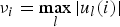 $\nu_{i}=\max_{\l} \vert u_{\l}\lpar i\rpar \vert $.
It is interesting to note that although the norm is not preserved when a kernel is localized on an arbitrary graph, it is preserved on average when translated to separately to every vertex on the graph:
 $$\eqalign{ {1 \over N}\sum_{i=1}^{N}\Vert T_{i}g\Vert _{2}^{2} & = \sum_{i=1}^{N}\sum_{\ell=0}^{N-1}\vert \hat{g}\lpar \lambda_{\ell}\rpar \bar{u}_{{\ell}}\lpar i\rpar \vert ^{2} \cr &= \sum_{\ell=0}^{N-1}\vert \hat{g}\lpar \lambda_{\ell}\rpar \vert ^{2}\sum_{i=1}^{N}\vert \bar{u}_{{\ell}}\lpar i\rpar \vert ^{2} = \Vert \hat{g}\Vert _{2}^{2}. }$$
The following example presents more precise insights on the interplay between the localization operator, the graph structure, and the concentration of localized functions.
Example 4
Figure 7 illustrates the effect of the graph structure on the norms of localized functions. We take the kernel to be localized to be a heat kernel of the form  $\hat{g}\lpar \lambda_{\ell}\rpar = e^{-\tau \lambda_{\ell}}$, for some constant τ > 0. We localize the kernel ĝ to be centered at each vertex i of the graph with the operator Ti, and we compute and plot their ℓ2-norms |Tig|2. The figure shows that when a center node i and its surrounding vertices are relatively weakly connected, the ℓ2-norm of the localized heat kernel is large, and when the nodes are relatively well connected, the norm is smaller. Therefore, the norm of the localized heat kernel may be seen as a measure of vertex centrality.Footnote 1 Moreover, in the case of the heat kernel, we can relate the ℓ2-norm of Ti g to its concentration s1(T1 g). Localized heat kernels are comprised entirely of non-negative components; i.e., $T_{i}g\lpar n\rpar \ge0$ for all i and n. This property comes from (i) the fact that $T_{i}g\lpar n\rpar =\lpar {\hat g}\lpar \cal L\rpar \rpar _{in}$ (see [Reference Hammond, Vandergheynst and Gribonval13]), and (ii) the non-trivial property that the entries of ${\hat g}\lpar {\cal}\rpar $ are always non-negative for the heat kernel [Reference Metzger and Stollmann63]. Since $T_{i}g\lpar n\rpar \ge 0$ for all i and n, we have
The heat kernel  ${\hat g}\lpar \lambda_{\ell}\rpar = e^{-10\lpar {\lambda_{\ell}}/{\lambda_{\rm max}\rpar } }$ (upper left), and the norms of the localized heat kernels, $\lcub \Vert T_{i}{g}\Vert _{2}\rcub _{i=1\comma 2\comma \ldots\comma N}$, on various graphs. For each graph and each center node i, the color of vertex i is proportional to the value of ‖Tig‖2. Within each graph, nodes i that are relatively less connected to their neighborhood seem to yield a larger norm ‖Tig‖2.

 $$\Vert T_ig\Vert _1= \sum_{n=1}^N T_i g\lpar n\rpar =\sqrt{N}\hat{g}\lpar 0\rpar =\sqrt{N}\comma$$
where the second equality follows from [23, Corollary 1]. Thus, recalling that a large value for s1(Ti g) means that Ti g is concentrated, we can combine (11) and (13) to derive an upper bound on the concentration of Ti g:
 $$s_1\lpar T_i g\rpar = \displaystyle{\Vert T_i g\Vert _2 \over \Vert T_i g\Vert _1}={\Vert T_i g\Vert _2 \over \sqrt{N}} \leq \nu_i \Vert \hat{g}\Vert _2.$$
Thus, ||Ti g||2 serves as a measure of concentration, and according to the numerical experiments of Fig. 7, localized heat kernels centered on the relatively well-connected regions of a graph tend to be less concentrated than the ones centered on relatively less well-connected areas. Intuitively, the values of the localized heat kernels can be linked to the diffusion of a unit of energy from the center vertex to surrounding vertices over a fixed time. In the well-connected regions of the graph, energy diffuses faster, making the localized heat kernels less concentrated.
The main class of dictionaries for graph signals that we consider is localized spectral graph filter frames.
Definition 4 (Localized spectral graph filter frame)
Let  $g=\lcub \widehat{g_{0}}\lpar{\cdot}\rpar \comma \; \widehat{g_{1}}\lpar{\cdot}\rpar \comma \; \ldots\comma \; \widehat{g_{K-1}}\lpar{\cdot}\rpar \rcub $ be a sequence of kernels (or filters), where each ${\hat g}_{k}\colon \sigma\lpar \cal L\rpar \to {\open C}$ is a function defined on the graph Laplacian spectrum $\sigma\lpar {\cal L}\rpar $ of a graph $\cal G$. Define the quantity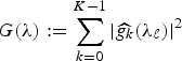 $G\lpar \lambda\rpar :=\sum_{k=0}^{K-1}\vert \widehat{g_{k}}\lpar \lambda_{\ell}\rpar \vert ^{2}$. Then ${\cal D}_{g}=\lcub g_{i\comma k}\rcub =\lcub T_{i} g_{k}\rcub $ is a localized spectral graph filter dictionary, and it forms a frame if $G\lpar \lambda\rpar \gt0$ for all $\lambda \in \sigma\lpar \cal L\rpar $.
In practice, each filter  $\widehat{g_{k}}\lpar{\cdot}\rpar $ is often defined as a continuous function over the interval $\lsqb 0\comma \; \lambda_{\max}\rsqb $ and then applied to the discrete set of eigenvalues in $\sigma\lpar \cal L\rpar $. The following lemma characterizes the frame bounds for a localized spectral graph filter frame.
Lemma 2 ([Reference Shuman, Wiesmeyr, Holighaus and Vandergheynst22], Lemma 1)
Let  ${\cal D}_{\rm g}=\lcub g_{i\comma k}\rcub =\lcub T_{i} g_{k}\rcub $ be a localized spectral graph filter frame of atoms on a graph $\cal G$ generated from the sequence of filters $\hbox{g}=\lcub \widehat{g_{0}}\lpar{\cdot}\rpar \comma \; \widehat{g_{1}}\lpar{\cdot}\rpar \comma \; \ldots\comma \; \widehat{g_{K-1}}\lpar{\cdot}\rpar \rcub $. The lower and upper frame bounds for ${\cal D}_{\rm g}$ are given by $A=N\cdot \min_{\lambda \in \sigma\lpar \cal L\rpar } G\lpar \lambda\rpar $ and $B=N\cdot \max_{\lambda \in \sigma\lpar \cal L\rpar } G\lpar \lambda\rpar $, respectively. If G(λ) is constant over $\sigma\lpar {\cal L}\rpar $, then ${\cal D}_{\rm g}$ is a tight frame.
Examples of localized spectral graph filter frames include the spectral graph wavelets of [Reference Hammond, Vandergheynst and Gribonval13], the Meyer-like tight graph wavelet frames of [Reference Leonardi and Van De Ville16,Reference Leonardi and Van De Ville64], the spectrum-adapted wavelets and vertex-frequency frames of [Reference Shuman, Wiesmeyr, Holighaus and Vandergheynst22], and the learned parametric dictionaries of [Reference Thanou, Shuman and Frossard65]. The dictionary constructions in [Reference Hammond, Vandergheynst and Gribonval13,Reference Shuman, Wiesmeyr, Holighaus and Vandergheynst22] choose the filters so that their energies are localized in different spectral bands. Different choices of filters lead to different tilings of the vertex-frequency space, and can for example lead to wavelet-like frames or vertex-frequency frames (analogous to classical windowed Fourier frames). The frame condition that G(λ) > 0 for all  $\lambda \in \sigma\lpar \L\rpar $ ensures that these filters cover the entire spectrum, so that no band of information is lost during analysis and reconstruction.
In this paper, in order to generalize classical windowed Fourier frames, we often use a localized graph spectral filter bank where the kernels are uniform translates, which we refer to as a graph Gabor filter bank.
Definition 5 (Graph Gabor filter bank)
When the K kernels used to generate the localized graph spectral filter frame are uniform translates of each otherFootnote 2, we refer to the resulting dictionary as a graph Gabor filter bank or a graph Gabor filter frame. If we use the warping technique of [Reference Shuman, Wiesmeyr, Holighaus and Vandergheynst22] on these uniform translatesFootnote 3, we refer to the resulting dictionary as a spectrum-adapted graph Gabor filter frame.
Graph Gabor filter banks are generalizations of the short time Fourier transform. When ĝ is smooth, the atoms are localized in the vertex domain [23, Theorem 1 and Corollary 2]. In this contribution, for all graph Gabor filter frames, we use the following mother window:  $\hat{g}\lpar t\rpar = \sin \lpar 0.5 \pi \cos \lpar \pi \lpar t-0.5\rpar \rpar^{2} \rpar \comma \; $ for $t\in \lsqb -0.5\comma \; 0.5\rsqb $ and 0 elsewhere. A few desirable properties of this choice of window are (a) it is perfectly localized in the spectral domain in [−0.5, 0.5], (b) it is smooth enough to be approximated by a low order polynomial, and (c) the frame formed by uniform translates (with an even overlap) is tight.
Definition 6 (Analysis operator)
The analysis operator of a dictionary  ${\cal D}=\lcub g_{i\comma k}\rcub $ to a signal $f \in {\cal C}^N$ is given by
 $${\cal A}_{\cal D} f\lpar i\comma \; k\rpar = \langle f\comma \; g_{i\comma k}\rangle.$$
 When  ${\cal D}=\lcub g_{i\comma k}\rcub =\lcub T_{i} g_{k}\rcub $ is a localized spectral graph filter frame, we denote it with ${\cal A}_{\rm g}$. In all cases, we view $A_{\cal D}$ as a function from ${\open C}^{N}$ to ${\open C}^{\vert {\cal D}\vert }$, and thus we use $\Vert{\cal A}_{\cal D} f\Vert_{p}$ (or $\Vert{\cal A}_{\rm g} f\Vert_{p}$) to denote a vector norm of the analysis coefficients.
V. GLOBAL UNCERTAINTY PRINCIPLES BOUNDING THE CONCENTRATION OF THE ANALYSIS COEFFICIENTS OF A GRAPH SIGNAL IN A TRANSFORM DOMAIN
Lieb's uncertainty principle in the continuous one- dimensional setting [Reference Lieb48] states that the cross-ambiguity function of a signal cannot be too concentrated in the time-frequency plane. In this section, we transpose these statements to the discrete periodic setting, and then generalize them to frames and signals on graphs.
A) Discrete version of Lieb's uncertainty principle
The following discrete version of Lieb's uncertainty principle is partially presented in [66, Proposition 2].
Theorem 3
Define the discrete Fourier transform (DFT) as
 $$\hat{f}\lsqb k\rsqb =\displaystyle{1 \over \sqrt{N}}\displaystyle\sum_{n=0}^{N-1}f\lsqb n\rsqb \exp\bigg({-i2\pi k n \over N}\bigg)\comma \;$$
and the discrete windowed Fourier transform (or discrete cross-ambiguity function) as (see, e.g., [Reference Mallat37, Section 4.2.3])
 $${{\cal A}_{\cal D}}_{DWFT} f\lsqb u\comma \; k\rsqb = \sum\limits_{n = 0}^{N - 1} f \lsqb n\rsqb \overline {g\lsqb n - u\rsqb } \exp \left({\displaystyle{{ - i2\pi kn} \over N}} \right).$$
For two discrete signals of period N, we have for  $2 \le p \lt \infty$
 $$\eqalign{ \Vert {{\cal A}_{\cal D}}_{DWFT} f \Vert _p &= \left(\sum_{u=1}^N \sum_{k=0}^{N-1} \vert {{\cal A}_{\cal D}}_{DWFT} f \lsqb u\comma \; k\rsqb \vert^p\right)^{{1 \over p}} \cr &\leq N^{1 \over p}\Vert f \Vert _2 \Vert g\Vert _2\comma \; }$$
and for 1 ≤ p ≤ 2
 $$\eqalign{ \Vert {{\cal A}_{\cal D}}_{DWFT} f \Vert _p &= \left(\sum_{u=1}^N \sum_{k=0}^{N-1} \vert {{\cal A}_{\cal D}}_{DWFT} f \lsqb u\comma \; k\rsqb \vert^p\right)^{{1 \over p}} \cr &\geq N^{1}/{p}\Vert f \Vert _2 \Vert g\Vert _2. }$$
These inequalities are proven in the Appendix. Note that the minimizers of this uncertainty principle are the so-called “picket fence” signals, trains of regularly spaced diracs.
B) Generalization of Lieb's uncertainty principle to frames
Theorem 4
Let  ${\cal D}=\lcub g_{i\comma k}\rcub $ be a frame of atoms in ${\open C}^{N}$, with lower and upper frame bounds A and B, respectively. For any signal $f \in {\open C}^{N}$ and any p ≥ 2, we have
 $$\Vert {\cal A}_{\cal D}f\Vert _{p}\leq B^{{1}/{p}}\lpar \max_{i\comma k}\Vert g_{i\comma k}\Vert_{2}\rpar ^{1-\lpar {2}/{p}\rpar }\Vert f\Vert _{2}.$$
For any signal  $f \in {\open C}^{N}$ and any 1 ≤ p ≤ 2, we have
 $$\Vert {\cal A}_{\cal D}f\Vert _{p}\geq A^{{1}/{p}}\lpar \max_{i\comma k}\Vert g_{i\comma k}\Vert_{2}\rpar ^{1-\lpar {2}/{p}\rpar }\Vert f\Vert _{2}.$$
Combining (16) and (17), for any  $p\in \lsqb 1\comma \; \infty\rsqb $, we have
 $$s_p\lpar {\cal A}_{\cal D}f\rpar \leq{B^{\min\lcub \lpar {1}/{2}\rpar \comma \lpar {1}/{p}\rpar \rcub } \over A^{\max\lcub {1}/{2}\comma {1}/{p}\rcub }}\lpar \max_{i\comma k}\Vert g_{i\comma k}\Vert_{2}\rpar ^{\vert 1-\lpar {2}/{p}\rpar \vert }.$$
When  $\cal D$ is a tight frame with frame bound A, (18) reduces to
 $$s_p\lpar {\cal A}_{\cal D}f\rpar \leq A^{-\vert \displaystyle\lpar {1}/{2}\rpar -\lpar {1}/{p}\rpar \vert }\lpar \max_{i\comma k}\Vert g_{i\comma k}\Vert _{2}\rpar ^{\vert 1-\lpar {2}/{p}\rpar \vert }.$$
A proof is included in the Appendix. The proof of Theorem 3 in the Appendix also demonstrates that this uncertainty principle is indeed a generalization of the discrete periodic variant of Lieb's uncertainty principle.
C) Lieb's uncertainty principle for localized spectral graph filter frames
Lemma 1 implies that
 $$\max_{i\comma k} {\Vert T_i g_k\Vert}_2 \leq \sqrt{N} \mu_{\cal G} \max_k {\Vert\widehat{g_k}\Vert}_2.$$
Therefore the following is a corollary to Theorem 4 for the case of localized spectral graph filter frames.
Theorem 5
Let  ${\cal D}_{\rm g}=\lcub g_{i\comma k}\rcub =\lcub T_{i} g_{k}\rcub $ be a localized spectral graph filter frame of atoms on a graph $\cal G$ generated from the sequence of filters $\hbox{g}=\lcub \widehat{g_{0}}\lpar{\cdot}\rpar \comma \; \widehat{g_{1}}\lpar{\cdot}\rpar \comma \; \ldots\comma \; \widehat{g_{K-1}}\lpar{\cdot}\rpar \rcub $. For any signal $f \in {\open C}^{N}$ on $\cal G$ and for any $p\in \lsqb 1\comma \; \infty\rsqb $, we have
 $$\eqalign{ s_p\lpar {\cal A}_{\rm g}f\rpar & \leq {B^{\min\lcub \lpar {1}/{2}\rpar \comma \lpar {1}/{p}\rpar \rcub } \over A^{\max\lcub \lpar {1}/{2}\rpar \comma \lpar {1}/{p}\rpar \rcub }}\lpar \max_{i\comma k}\Vert g_{i\comma k}\Vert_{2}\rpar ^{\vert 1-\lpar {2}/{p}\rpar \vert } \cr &\leq {B^{\min\lcub \lpar {1}/{2}\rpar \comma \lpar {1}/{p}\rpar \rcub } \over A^{\max\lcub \lpar {1}/{2}\rpar \comma \lpar {1}/{p}\rpar \rcub }}\left(\sqrt{N}\mu_{\cal G} \max_{k}\Vert \widehat{g_k}\Vert_{2}\right)^{\vert 1-\lpar {2}/{p}\rpar \vert }\comma \; }$$
where 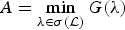 $A=\min_{\lambda \in \sigma\lpar \cal L\rpar } G\lpar \lambda\rpar $ is the lower frame bound and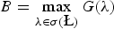 $B=\max_{\lambda \in \sigma\lpar \L\rpar } G\lpar \lambda\rpar $ is the upper frame bound. When $\cal D$ is a tight frame with frame bound A, (19) reduces to
 $$\eqalign{ s_p\lpar {\cal A}_{\rm g}f\rpar &\leq A^{-\vert \lpar {1}/{2}\rpar -\lpar {1}/{p}\rpar \vert }\lpar \max_{i\comma k}\Vert g_{i\comma k}\Vert_{2}\rpar ^{\vert 1-\lpar {2}/{p}\rpar \vert } \cr &\leq A^{-\vert \lpar {1}/{2}\rpar -\lpar {1}/{p}\rpar \vert }\left(\sqrt{N}\mu_{\cal G} \max_{k}\Vert \widehat{g_k}\Vert_{2}\right)^{\vert 1-\lpar {2}/{p}\rpar \vert }. }$$
 The bounds depend on the frame bounds A and B, which are fixed with the design of the filter bank. However, in the tight frame case, we can choose the filters in a manner such that the bound A does not depend on the graph structure. For example, if the  ${\hat g}_k$ are defined continuously on the interval $\lsqb 0\comma \; \lambda_{\rm max}\rsqb $ and $\sum_{k=0}^{M-1}\vert {\hat g}_{k}\lpar \lambda\rpar \vert ^{2}$ is equal to a constant for all λ, A is not affected by a change in the values of the Laplacian eigenvalues, e.g., from a change in the graph structure. The second quantity, $\max_{i\comma k}\Vert g_{i\comma k}\Vert _{2}$, reveals the influence of the graph. The maximum ℓ2-norm of the atoms depends on the filter design, but also, as discussed previously in Section IV, on the graph topology. However, the bound is not local as it depends on the maximum |g i, k|2 over all localizations i and filters k, which takes into account the entire graph structure.
The second bounds in (19) and (20) also suggest how the filters can be designed so as to improve the uncertainty bound. The quantity  $\Vert \widehat{g_{k}}\Vert _{2} = \lpar \sum_{\ell} \vert {\hat g}_{k}\lpar \lambda_{\ell}\rpar \vert ^{2} \rpar $ depends on the distribution of the eigenvalues $\lambda_{\ell}$, and, as a consequence, on the graph structure. However, the distribution of the eigenvalues can be taken into account when designing the filters in order to reduce or cancel this dependency [Reference Shuman, Wiesmeyr, Holighaus and Vandergheynst22].
In the following example, we compute the first uncertainty bound in (20) for different types of graphs and filters. It provides some insight on the influence of the graph topology and filter bank design on the uncertainty bound.
Example 5
We use the techniques of [Reference Shuman, Wiesmeyr, Holighaus and Vandergheynst22] to construct four tight localized spectral graph filter frames for each of eight different graphs. Figure 8 shows an examples of the four sets of filters for a 64 node sensor network. For each graph, two of the sets of filters (b and d in Fig. 8) are adapted via warping to the distribution of the graph Laplacian eigenvalues so that each filter contains an appropriate number of eigenvalues (roughly equal in the case of translates and roughly logarithmic in the case of wavelets). The warping avoids filters containing zero or very few eigenvalues at which the filter has a non-zero value. These tight frames are designed such that A = N, and thus Theorem 5 yields
Four different filter bank designs of [22], shown for a random sensor network with 64 nodes. Each colored curve is a filter defined continuously on  $\lsqb 0\comma \; \lambda_{\rm max}\rsqb $, and each filter bank has 16 such filters. They are designed such that $G\lpar \lambda\rpar =1$ for all λ (black line), and thus all four designs yield tight localized spectral graph filter frames. The frame bounds here are A = B = N.

 $$\eqalign{ s_{\infty}\lpar {\cal A}_{\rm g}f\rpar ={\Vert {\cal A}_{\rm g}f\Vert _\infty \over \Vert {\cal A}_{\rm g}f\Vert _2} & \leq { N^{-\lpar {1}/{2}\rpar }} \max_{i\comma k}\Vert T_ig_k\Vert _2 \cr &\leq \mu_{\cal G}\max_k \Vert \widehat{g_k}\Vert _2.}$$
Table 1 displays the values of the first concentration bound  $\max_{i\comma k}\Vert T_{i}g_{k}\Vert _{2}$ for each graph and frame pair. The uncertainty bound is largest when the graph is far from a regular lattice (ring or path). As expected, the worst cases are for highly inhomogeneous graphs like the comet graph or a modified path graph with one isolated vertex. {Note also that the coherence $\mu_{\cal G}$ is very large (0.90) for the random sensor network. Because of randomness, there is a high probability that one node will be isolated, hence creating a large coherence. The choice of the filter bank may also decrease or increase the bound, depending on the graph.
The uncertainty principle in Theorem 5 bounds the concentration of the graph Gabor transform coefficients. In the next example, we examine these coefficients for a series of signals with different vertex and spectral domain localization properties.
Example 6 (Concentration of the graph Gabor coefficients for signals with varying vertex and spectral domain concentrations.)
In Fig. 9, we analyze a series of signals on a random sensor network of 100 vertices. Each signal is created by localizing a kernel  $\widehat{h_{\tau}}\lpar \lambda\rpar = e^{-\lpar {\lambda^{2}}/{\lambda_{\rm max}^{2}} \rpar \tau^{2}}$ to be centered at vertex 1 (circled in black). To generate the four different signals, we vary the value of the parameter τ in the heat kernel. We plot the four localized kernels in the graph spectral and vertex domains in the first two columns, respectively. The more we “compress” ĥ in the graph spectral domain (i.e. we reduce its spectral spreading by increasing τ), the less concentrated the localized atom becomes in the vertex domain. The joint vertex-frequency representation $\vert {\cal A}_{\rm g} T_{1}h_{\tau}\lpar i\comma \; k\rpar \vert $ of each signal is shown in the third column, which illustrates the trade-off between concentration in the vertex and the spectral domains. The concentration of these graph Gabor transform coefficients is the quantity bounded by the uncertainty principle presented in Theorem 5. In the last row of the Fig. 9, τ = ∞ which leads to a Kronecker delta for the kernel and a constant on the vertex domain. On the contrary, when the kernel is constant, with τ = 0 (top row), the energy of the graph Gabor coefficients stays concentrated around one vertex but spreads along all frequencies.
Graph Gabor transform of four different signals  $f_{\tau}=T_{1} h_{\tau}$, with each row corresponding to a signal with a different value of the parameter τ. Each of the signals is a kernel localized to vertex 1, with the kernel to be localized equal to $\widehat{h_{\tau}}\lpar \lambda\rpar =e^{-\lpar {\lambda^{2}}/{\lambda_{{\rm max}}^{2}\rpar } \tau^{2}}$. The underlying graph is a random sensor network of 100 vertices. First column: the kernel $h_{\tau}\lpar \lambda\rpar $ is shown in red and the localized kernel $\widehat{f_{\tau}}$ is shown in blue, both in the graph spectral domain. Second column: the signal fτ in the vertex domain (the center vertex 1 is circled). Third column: $\vert {\cal A}_{\rm g} T_{1}h_{\tau} \lpar i\comma \; k\rpar \vert $, the absolute value of the Gabor transform coefficients for each vertex i and each of the 20 frequency bands k. Fourth column: since it is hard to see where on the graph the transform coefficients are concentrated when the nodes are placed on a line in the third column, we display the value $\sum_{k=0}^{19} \vert {\cal A}_{\rm g} T_{1}h_{\tau} \lpar i\comma \; k\rpar \vert $ on each vertex i in the network. This figure illustrates the tradeoff between the vertex and the frequency concentration.

VI. LOCAL UNCERTAINTY PRINCIPLES FOR SIGNALS ON GRAPHS
In the previous section, we defined a global bound for the concentration of the localized spectral graph filter frame analysis coefficients. In the classical setting, such a global bound is also local in the sense that each part of the domain has the same structure, due to the regularity of the underlying domain. However, this is not the case for the graph setting where the domain is irregular. Example 1 shows that a “bad” structure (a weakly connected node) in a small region of the graph reduces the uncertainty bound even if the rest of the graph is well behaved. Functions localized near the weakly connected node can be highly concentrated in both the vertex and frequency domains, whereas functions localized away from it are barely impacted. Importantly, the worst case determines the global uncertainty bound. As another example, suppose one has two graphs G 1 and G 2 with two different structures, each of them having a different uncertainty bound. The uncertainty bound for the graph  $\cal G$ that is the union of these two disconnected graphs is the minimum of the uncertainty bounds of the two disconnected graphs, which is suboptimal for one of the two graphs.
In this section, we ask the following questions. Where does this worse case happen? Can we find a local principle that more accurately characterizes the uncertainty in other parts of the graph? In order to answer this question, we investigate the concentration of the analysis coefficients of the frame atoms, which are localized signals in the vertex domain. This technique is used in the classical continuous case by Lieb [Reference Lieb48], who defines the (cross-) ambiguity function, the STFT of a short-time Fourier atom. The result is a joint time-frequency uncertainty principle that does not depend on the localization in time or in frequency of the analyzed atom.
Thus, we start by generalizing to the graph setting the definition of ambiguity (or cross-ambiguity) functions from time-frequency analysis of one-dimensional signals.
Definition 7 (Ambiguity function)
The ambiguity function of a localized spectral frame  ${\cal D}=\lcub g_{i\comma k}\rcub =\lcub T_{i} g_{k}\rcub $ is defined as:
 $${\open A}_{\rm g}\lpar i_0\comma \; k_0\comma \; i\comma \; k\rpar = {\cal A}_{\rm g} T_{i_0} g_{k_0} \lpar i\comma \; k\rpar = \langle T_{i_0} g_{k_0} \comma \; T_i g_k \rangle$$
 When the kernels  $\lcub \widehat{g_{k}}\rcub _{k=0\comma 1\comma \ldots\comma M-1}$ are appropriately warped uniform translates, the operator ${\open A}_{\rm g}$ becomes a generalization of the short-time Fourier transform. Additionally, the ambiguity function assesses the degree of coherence (linear dependence) between the atoms $T_{i_{0}} g_{k_{0}}$ and T i g k. In the following, we use this ambiguity function to probe locally the structure of the graph, and derive local uncertainty principles.
A) Local uncertainty principle
In order to probe the local uncertainty of a graph, we take a set of localized kernels in the graph spectral domain and center them at different local regions of the graph in the vertex domain. The atoms resulting from this construction are jointly localized in both the vertex and graph spectral domains, where “localized” means that the values of the function are zero or close to zero away from some reference point. By ensuring that the atoms are localized or have support within a small region of the graph, we focus on the properties of the graph in that region. In order to get a local uncertainty principle, we apply the frame operator to these localized atoms, and analyze the concentration of the resulting coefficients. In doing so, we develop an uncertainty principle relating these concentrations to the local graph structure.
To prepare for the theorem, we first state a lemma that gives a hint to how the scalar product of two localized functions depends on the graph structure and properties. In the following, we multiply two kernels ĝ and ĥ in the graph spectral domain. For notation, we represent the product of these two kernels in vertex domain as g·h.
Lemma 3
For two kernels ĝ, ĥ and two nodes i, j, the localization operator satisfies
 $$\langle T_{i}g\comma \; T_{j}h\rangle = \sqrt{N}T_{i}\lpar g\cdot h\rpar \lpar j\rpar \comma$$
and
 $$\bigg(\sum_{i}\vert \langle T_{i}g\comma \; T_{j}h \rangle \vert ^{p}\bigg)^{{1}/{p}}=\sqrt{N}\Vert T_{j}\lpar g\cdot h\rpar \Vert _{p}.$$
 Equation (21) shows more clearly the conditions on the kernels and nodes under which the scalar product is small. Let us take two examples. First, suppose  ${\hat g}$ and ${\hat h}$ have a compact support on the spectrum and do not overlap (kernels localized in different places), then ${\hat g} \cdot\semicolon \; {\hat h}$ is zero everywhere on the spectrum, and therefore the scalar product on the left-hand side of (21) is also equal to zero. Second, assume i and j are distant from each other. Then $\vert T_{i}\lpar g\cdot h\rpar \lpar j\rpar \vert $ is small if ĝ and ĥ are reasonably smooth. In other words, the two atoms T i g and T j h must be localized both in the same area of graph in the vertex domain and the same spectral region in order for the scalar product to be large. This localization depends on the atoms, but also on the graph structure.
Proof of Lemma 3:
 $$\eqalign{ &\langle T_{i}g\comma \; T_{j}h \rangle \cr &\quad= \langle \widehat{T_{i}g}\comma \; \widehat{T_{j}h} \rangle = N\sum_{\ell=0}^{N-1}\hat{g}\lpar \lambda_{\ell}\rpar u_{\ell}\lpar i\rpar \bar{\hat{h}}\lpar \lambda_{\ell}\rpar \bar{u}_{\ell}\lpar j\rpar \cr &\quad= N\sum_{\ell=0}^{N-1}\lpar \hat{g}\cdot \hat{h}\rpar \lpar \lambda_{\ell}\rpar u_{\ell}\lpar i\rpar \bar{u}_{\ell}\lpar j\rpar = \sqrt{N}T_{i}\lpar g\cdot h\rpar \lpar j\rpar .}$$
Moreover, a direct computation shows
 $$\eqalign{&\bigg(\sum_{i}\vert \langle T_{i}g\comma \; T_{j}h \rangle \vert ^{p}\bigg)^{{1}/{p}} \cr &\quad=\bigg(\sum_{i}\left\vert \sqrt{N}T_{j}\lpar g\cdot h\rpar \lpar i\rpar \right\vert ^{p}\bigg)^{{1}/{p}}=N^{{1}/{2}}\Vert T_{j}\lpar g\cdot h\rpar \Vert _{p}. \square}$$
 The inequalities in the following theorem constitute a local uncertainty principle. The local bound depends on the localization of the atom  $T_{i_{0}}g_{k_{0}}$ in the vertex and spectral domains. The center vertex i 0 and kernel $\hat{g}_{k_{0}}$ can be chosen to be any vertex and kernel; however, the locality property of the uncertainty principle appears when $T_{i_{0}}g_{k_{0}}$ is concentrated around node i 0 in the vertex domain and around a small portion of the spectrum in the graph spectral domain. We again measure the concentration with ℓp-norms.
Theorem 6 (Local uncertainty)
Let  $\lcub T_{i}g_{k} \rcub _{\lcub i\in\lsqb 1\comma N\rsqb \comma k\in\lsqb 0\comma M-1\rsqb \rcub }$ be a localized spectral graph filter frame with lower frame bound A and upper frame bound B. For any $i_{0}\in\lsqb 1\comma \; N\rsqb \comma \; k_{0}\in\lsqb 0\comma \; M-1\rsqb $ such that $\Vert T_{i_{0}}g_{k_{0}}\Vert _{2}>0$, the quantity
 $$\eqalign{ \Vert {\cal A}_{\rm g}T_{i_0}g_{k_0}\Vert _{p} &= \bigg(\sum_{k=1}^{M}\sum_{i=1}^{N}\vert \langle T_{i}g_{k}\comma \; T_{i_{0}}g_{k_{0}} \rangle \vert ^{p}\bigg)^{{1}/{p}} \cr &= \sqrt{N}\bigg(\sum_{k=1}^{M}\Vert T_{i_0}\lpar g_{k_0}\cdot g_{k}\rpar \Vert _{p}^{p}\bigg)^{{1}/{p}}\comma \; }$$
satisfies for  $p \in \lsqb 1\comma \; \infty\rsqb $
 $$\eqalign{ & s_p\lpar {\cal A}_{\rm g}T_{i_0}g_{k_0}\rpar \cr &\quad \leq{B^{\min\lcub \lpar {1}/{p}\rpar \comma 1-\lpar {1}/{p}\rpar \rcub }\Vert T_{\tilde{i}_{i_0\comma k_0}}g_{\tilde{k}_{i_0\comma k_0}}\Vert _{2}^{\vert 1-\lpar {2}/{p}\rpar \vert } \over A^{{1}/{2}}} \cr &\quad \leq { B^{\min\lcub \lpar {1}/{p}\rpar \comma 1-\lpar {1}/{p}\rpar \rcub } \lpar \sqrt{N}\nu_{\tilde{i}_{i_0\comma k_0}} \Vert g_{\tilde{k}_{i_0\comma k_0}} \Vert _2 \rpar ^{\vert 1-\lpar {2}/{p}\rpar \vert } \over A^{{1}/{2}}}\comma \; }$$
where νi is defined in Lemma 1,
 $$\eqalign{\tilde{k}_{i_0\comma k_0}&=\arg\, \max_{k}\Vert T_{i_0}\lpar g_{k_0}\cdot g_{k}\rpar \Vert _{\infty}\comma \; \hbox{and} \cr \tilde{i}_{i_0\comma k_0}&=\arg\, \max_{i}\vert T_{i_0}\lpar g_{k_0}\cdot g_{\tilde{k}_{i_0\comma k_0}}\rpar \lpar i\rpar \vert .}$$
 The bound in (24) is local, because we get a different bound for each i 0, k 0 pair. For each such pair, the bound depends on the quantities  $\tilde{i}_{i_{0}\comma k_{0}}\comma \; \tilde{k}_{i_{0}\comma k_{0}}$, which are maximizers over a set of all vertices and kernels, respectively; however, as we discuss in Example 7 below, $\tilde{i}_{i_{0}\comma k_{0}}$ is typically close to i 0, and $\tilde{k}_{i_{0}\comma k_{0}}$ is typically close to k 0. For this reason, this bound typically depends only on local quantities.
Proof [Proof of Theorem 6] For notational brevity in this proof, we omit the indices i 0, k 0 for the quantities ĩ and  $\tilde{k}$. First, note that
 $$\eqalign{\Vert {\cal A}_{\rm g}T_{i_0}g_{k_0}\Vert _{\infty} &= \max_{k}\sqrt{N}\Vert T_{i_0}\lpar g_{k_0}\cdot g_{k}\rpar \Vert _{\infty} \cr &\leq\Vert T_{\tilde{i}}g_{\tilde{k}}\Vert _{2}\Vert T_{i_0}g_{k_0}\Vert _{2}\comma \; }$$
where  $\tilde{k}_{i_{0}\comma k_{0}}\, =\, \hbox{arg max}_{k}\, \Vert T_{i_{0}}\lpar g_{k_{0}}\, {\cdot}\, g_{k}\rpar \Vert _{\infty}$ and $\tilde{i}_{i_{0}\comma k_{0}}\, = \hbox{arg min}_{i} \vert T_{i_{0}}\lpar g_{k_{0}}\cdot g_{\tilde{k}}\rpar \lpar i\rpar \vert $. Let us then interpolate the two following expressions:
 $$\Vert {\cal A}_{\rm g}T_{i_0}g_{k_0}\Vert _{2}\leq B^{{1 \over 2}}\Vert T_{i_0}g_{k_0}\Vert _{2}$$
 $$\hbox{and} \quad \Vert {\cal A}_{\rm g}T_{i_0}g_{k_0}\Vert _{\infty}\le\Vert T_{\tilde{i}}g_{\tilde{k}}\Vert _{2}\Vert T_{i_0}g_{k_0}\Vert _{2}.$$
We use the Riesz–Thorin Theorem (Theorem 8) with  $p_{1}=q_{1}=p_{2}=2$, q 2 = ∞, $M_{p}=B^{{1 \over 2}}$ and $M_{q}=\Vert T_{\tilde{i}}g_{\tilde{k}}\Vert _{2}$. Note that ${\cal A}_{\rm g}$ is a bounded operator from the Hilbert space spanned by $T_{i_{0}}g_{k_{0}}$ (isomorphic to a one-dimensional Hilbert space) to the one spanned by $\lcub T_{i_{0}}g_{k_{0}}\rcub _{i\comma k}$. We take t = 2/r 2 and find r 1 = 2, leading to
 $$\Vert {\cal A}_{\rm g}T_{i_0}g_{k_0}\Vert _{r_{2}}\le B^{{1}/{r_{2}}}\Vert T_{\tilde{i}}g_{\tilde{k}}\Vert _{2}^{1-\lpar {2}/{r_{2}\rpar }}\Vert T_{i_0}g_{k_0}\Vert _{2}.$$
 Since  ${\cal A}_{\rm g}$ is a frame, we also have $\Vert {\cal A}_{\rm g}T_{i_{0}}g_{k_{0}}\Vert _{2}\ge A^{{1 \over 2}}\Vert T_{i_{0}} g_{k_{0}}\Vert _{2}$, which yields:
 $${\Vert {\cal A}_{\rm g}T_{i_0}g_{k_0}\Vert _{2} \over \Vert {\cal A}_{\rm g}T_{i_0}g_{k_0}\Vert _{p}}\ge{A^{{1}/{2}} \over B^{{1 \over p}}\Vert T_{\tilde{i}}g_{\tilde{k}}\Vert _{2}^{1-\lpar {2}/{p}\rpar }}.$$
 Finally, thanks to Hölder's inequality, we have for p ≤ 2 and  $\lpar {1}/{p}\rpar +\lpar {1}/{q}\rpar =1$
 $$\eqalign{{\Vert {\cal A}_{\rm g}T_{i_0}g_{k_0}\Vert _{2} \over \Vert {\cal A}_{\rm g}T_{i_0}g_{k_0}\Vert _{p}} &\leq {\Vert {\cal A}_{\rm g}T_{i_0}g_{k_0}\Vert _{q} \over \Vert {\cal A}_{\rm g}T_{i_0}g_{k_0}\Vert _{2}} \cr &\leq {B^{{1}/{q}}\Vert T_{\tilde{i}}g_{\tilde{k}}\Vert _{2}^{1-\lpar {2}/{p}\rpar } \over A^{{1}/{2}}} \cr &\leq {B^{1-\lpar {1}/{p}\rpar }\Vert T_{\tilde{i}}g_{\tilde{k}}\Vert _{2}^{\lpar {2}/{p}\rpar -1} \over A^{{1 \over 2}}} \cr &\leq { B^{1-\lpar {1}/{p}\rpar } \lpar \sqrt{N}\nu_{\tilde{i}} \Vert g_{\tilde{k}} \Vert _2 \rpar ^{\lpar {2}/{p}\rpar -1} \over A^{{1}/{2}}}. \square}$$
 The next corollary shows that in many cases, the local uncertainty inequality (24) is sharp (becomes an equality). To obtain this, we require that the frame  ${\cal A}_{\rm g}$ is tight and $\vert \langle T_{i}g_{k}\comma \; T_{i_{0}}g_{k_{0}} \rangle\vert $ is maximized when k = k 0 and i = i 0.
Corollary 2
Under the assumptions of Theorem 6 and, assuming additionally
(i)
${\cal A}_{\rm g}$ is a tight frame with frame-bound A,(ii)
$k_{0} = \hbox{arg max}_{k} \Vert T_{i_{0}}\lpar g_{k}\cdot g_{k_{0}}\rpar \Vert _{\infty}$, and(iii)
$i_{0} = \hbox{arg max}_{j} \vert T_{i_{0}}g_{k_{0}}^{2}\lpar j\rpar \vert $,



we have
 $$s_\infty\lpar {\cal A}_{\rm g}T_{i_0}g_{k_0}\rpar = {\Vert {\cal A}_{\rm g}T_{i_0}g_{k_0}\Vert _{\infty} \over \Vert {\cal A}_{\rm g}T_{i_0}g_{k_0} \Vert _{2}} = {\Vert T_{i_0} g_{k_0} \Vert _{2} \over A^{{1 \over 2}}}.$$
Proof The proof follows directly from the two following equalities. For the denominators, since the frame is tight, we have:
 $$\Vert {\cal A}_{\rm g}T_{i_0}g_{k_0}\Vert _{2} = A^{{1 \over 2}}\Vert T_{i_0}g_{k_0}\Vert _{2}.$$
For the numerators, we have
 $$\eqalign{ {\rm \Vert }A_{\rm g}T_{i_0}g_{k_0}{\rm \Vert }_\infty &= \max _{i\comma k}\vert \langle{T_ig_kT_{i_0}g_{k_0}} \rangle \vert \cr &= \sqrt N \max _{i\comma k}\vert T_{i_0}\lpar g_k\cdot g_{k_0}\rpar \lpar i\rpar \vert }$$
 $$\eqalign{ &= \sqrt{N}\max_{k} \Vert T_{i_0}\lpar g_{k}\cdot g_{k_0}\rpar \Vert _\infty \cr &= \sqrt{N}\Vert T_{i_0} g_{k_0}^2\Vert _\infty }$$
 $$= \sqrt{N}\vert T_{i_0}g_{k_0}^2\lpar i_0\rpar \vert$$
 $$\eqalign{ &= \langle{T_{i_0}g_{k_0} }\comma \; {T_{i_0} g_{k_0} }\rangle \cr &= \Vert {T_{i_0}g_{k_0}\Vert _{2}^{2} }}$$
where (28) and (31) follow from (21), (29) follows from the second hypothesis, and (30) follows from the third hypothesis.□
Corollary 3
Under the assumptions of Theorem 6, we have
 $$\eqalign{ s_\infty\lpar {\cal A}_{\rm g}T_{i_{0}}g_{k_{0}}\rpar = {\Vert {\cal A}_{\rm g}T_{i_{0}}g_{k_{0}}\Vert _{\infty} \over \Vert {\cal A}_{\rm g}T_{i_{0}}g_{k_{0}}\Vert _{2}}\geq {\Vert T_{i_{0}}g_{k_{0}}\Vert _{2} \over B^{{1 \over 2}}} \comma \; }$$
which is a lower bound on the concentration measure.
Proof We have
 $$\eqalign{ \Vert {\cal A}_{\rm g}T_{i_{0}}g_{k_{0}}\Vert _{\infty}&= \max_{i\comma k} \vert \langle{T_{i}g_{k}}{T_{i_0}g_{k_0}}\rangle \vert \cr & \geq \vert \langle{T_{i_{0}}g_{k_{0}}}{T_{i_{0}}g_{k_{0}}}\rangle\vert = \Vert T_{i_{0}}g_{k_{0}}\Vert _{2}^{2}. }$$
 Additionally, because  $\lcub T_{i} g_{k}\rcub _{i=1\comma 2\comma \ldots\comma N\semicolon k=0\comma 1\comma \ldots\comma M-1}$ is a frame, we have
 $$\eqalign{ \Vert {\cal A}_{\rm g}T_{i_{0}}g_{k_{0}}\Vert _{2}\leq B^{{1}/{2}}\Vert T_{i_{0}}g_{k_{0}}\Vert _{2}. }$$
Combining (33) and (34) yields the desired inequality in (32). □
Together, Theorem 6 and Corollary 3 yield lower and upper bounds on the local sparsity levels  $s_{\infty}\lpar {\cal A}_{\rm g}T_{i_{0}}g_{k_{0}}\rpar $:
 $$\eqalign{\displaystyle{{\Vert T_{\tilde{i}}g_{\tilde{k}}\Vert _{2}}\over{A^{\displaystyle{{1}\over{2}}}}} & \ge s_\infty\lpar {\cal A}_{\rm g}T_{i_{0}}g_{k_{0}}\rpar \cr & = \displaystyle{{\Vert {\cal A}_{\rm g}T_{i_{0}}g_{k_{0}}\Vert _{\infty}}\over{\Vert {\cal A}_{\rm g}T_{i_{0}}g_{k_{0}}\Vert _{2}}}\ge \displaystyle{{\Vert T_{i_{0}}g_{k_{0}}\Vert _{2}}\over{B^{\displaystyle{{1}\over{2}}}}}.}$$
B) Illustrative examples
In order to better understand this local uncertainty principle, we illustrate it with some examples.
Example 7 [Local uncertainty on a sensor network]
Let us concentrate on the case where p = ∞. Theorem 6 tells us that
 $$\eqalign{\displaystyle{{\Vert {\cal A}_{\rm g}T_{i_0}g_{k_0}\Vert _{\infty}}\over{\Vert {\cal A}_{\rm g}T_{i_0}g_{k_0}\Vert _{2}}} & \leq \displaystyle{{\Vert T_{\tilde{i}_{i_0\comma k_0}}g_{\tilde{k}_{i_0\comma k_0}}\Vert _{2}}\over{A^{\displaystyle{{1}\over{2}}}}} \cr & \leq \displaystyle{{ \lpar \sqrt{N}\nu_{\tilde{i}_{i_0\comma k_0}} \Vert g_{\tilde{k}_{i_0\comma k_0}} \Vert _2 \rpar }\over{A^{\displaystyle{{1}\over{2}}}}}\comma \; }$$
meaning that the concentration of  ${\cal A}_{\rm g}T_{i_{0}}g_{k_{0}}$ is limited by ${1}/{\Vert T_{\tilde{i}}g_{\tilde{k}_{i_{0}\comma k_{0}}}\Vert _{2}}$. One question is to what extent this quantity is local or reflects the local behavior of the graph. As a general illustration for this discussion, we present in Fig. 10 quantities related to the local uncertainty of a random sensor network of 100 nodes evaluated for two different values of k (one in each column) and all nodes i.
Illustration of Theorem 6 and related variables ĩ and  $\tilde{k}$ for a random sensor graph of 100 nodes. Top figure: the 8 uniformly translated kernels $\lcub \widehat{g_{k}}\rcub _{k}$ (in 8 different colors) defined on the spectrum and giving a tight frame. Each row corresponds to quantities related to the local uncertainty principle. The first column concerns the kernel (filter) in blue on the top figure, the second is associated with the orange one. On a sensor graph, the local uncertainty level (inversely proportional to the local sparsity level plotted here) is far from constant from one node to another or from one frequency band to another.

The first row (not counting the top figure) shows the local sparsity levels of  ${\cal A}_{\rm g}T_{i_{0}}g_{k_{0}}$ in terms of the ℓ∞-norm (left hand side of (35)) at each node of the graph. The second row shows the values of the upper bound on local sparsity for each node of the graph (middle term of (35)). The values of both rows are strikingly close. Note that for this type of graph, local sparsity/concentration is lowest where the nodes are well connected.
We focus now on the values of  $\tilde{k}$ and ĩ as they are crucial in Theorem 6. We also give insights that explain when a tight bound is obtained, as stated in Corollary 2. There is not a simple way to determine the value of $\tilde{k}$, because it depends not only on the node i0 and the filters $\widehat{g_{k}}$, but also on the graph Fourier basis. However, the definition $\tilde{k} = {argmax}_{k} \Vert T_{i_{0}}\lpar g_{k}\cdot g_{k_{0}}\rpar \Vert _{\infty}$ implies that the two kernels $\widehat{g_{\tilde{k}}}$ and $\widehat{g_{k_{0}}}$ have to overlap “as much as possible” in the graph Fourier domain in order to maximize the infinity-norm. In the case of a Gabor filter bank like the one presented in the first line of Fig. 10, $k_0={\tilde{k}}$ for most of the nodes. This happens because the filters $\widehat{g_{k}}$ and $\widehat{g_{k_{0}}}$ do not overlap much if k ≠ k0, i.e when
 $$\eqalign{\Vert \widehat{g_{k_{0}}}^{2}\Vert _{2}^{2} & =\sum_{\ell}\lpar \widehat{g_{k_{0}}}^{2}\lpar \lambda_\ell\rpar \rpar ^{2} \cr & \gg \sum_{\ell}\lpar \widehat{g_{k_{0}}}\lpar \lambda_\ell\rpar \widehat{g_{k}}\lpar \lambda_\ell\rpar \rpar ^{2}=\Vert \widehat{g_{k}}\cdot \widehat{g_{k_{0}}}\Vert _{2}^{2}.}$$
 In fact, in the case of Fig. 10,  $\tilde{k}$ is bounded between k0 − 1 and k0 + 1 because there is no overlap with the other filters. In Fig. 10, we plot ${\tilde{k}}(i)$ for k0 = 0 and k0 = 1. For the first filter, we have $\tilde{k}_{i_{0}\comma k_{0}} = k_{0}$ for all vertices i0. The second filter follows the same rule except for two nodes. The isolated node on the north east is less connected to the rest and there is a Laplacian eigenvector well localized on it. As a consequence, the localization on the graph is affected in a counter-intuitive manner.
Let us now concentrate on the second important variable: ĩ. Under the assumption that the kernels  $\widehat{g_{k}}$ are smooth, the energy of localized atoms $T_{i_{0}}g_{k}$ reside inside a ball centered at i0 [Reference Shuman, Ricaud and Vandergheynst23]. Thus, the node j maximizing $\vert T_{i_{0}}\lpar g_{k_{0}} g_{\tilde{k}}\rpar \lpar j\rpar \vert$ cannot be far from the node i0. Let us define the hop distance $h_{\cal G}\lpar i\comma \; j\rpar $ as the length of the shortest pathFootnote 4 between nodes i and j. If the kernels $\widehat{g_{k}}$ are polynomial functions of order K, the localization operator $T_{i_{0}}$ concentrates all of the energy of $T_{i_{0}}g_{k}$ inside a K-radius ball centered in i0. Since the resulting kernel $\widehat{g_{k_{0}}} \widehat{g_{\tilde{k}}}$ is a polynomial of order 2K, ĩ will be at a distance of at most of 2K hops from the node i0. In general, ĩ is close to i0. In fact, the distance $h_{\cal G}\lpar i\comma \; \tilde{i}\rpar$ is related to the smoothness of the kernel $\widehat{g_{k_{0}}}\widehat{g_{\tilde{k}}}$ [Reference Shuman, Ricaud and Vandergheynst23]. To illustrate this effect, we present in Fig. 11 the average and maximum hop distance $h_{\cal G}\lpar i\comma \; \tilde{i}\rpar $. In this example, we control the concentration of a kernel ${\hat g}$ with a dilation parameter a: $\widehat{g_{a}}\lpar x\rpar = {\hat g}\lpar ax\rpar $. Increasing the factor a compresses the kernel in the Fourier domain and increases the spread of the localized atoms in the vertex domain. Note that even for high spectral compression, the hop distance $h_{\cal G}\lpar i\comma \; \tilde{i}\rpar$ remains low. Additionally, we also compute the mean relative error between $\Vert T_{i} g^{2} \Vert _{\infty}$ and $\vert T_{i} g^{2}\lpar i\rpar \vert $. This quantity asserts how well $\Vert T_{i} g \Vert _{2}^{2}$ estimates $\Vert T_{i} g^{2} \Vert _{\infty}$.Footnote 5 Returning to Fig. 10, the fourth row shows the hop distance between i0 and ĩ. It never exceeds 3 for both the first and the second filter, so $\tilde{i}_{k_{0}\comma i_{0}}$ is close to i0.
Localization experiment using the sensor graph of Fig. 10. The heat kernel (top) is defined as 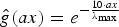 ${\hat g}\lpar ax\rpar = e^{-{{10 \cdot ax}\over{\lambda_{\rm max}}}}$ and the wavelet kernel (middle) is defined as ${\hat g}\lpar ax\rpar = \sqrt{40} \cdot ax \cdot e^{-{{40\cdot ax}\over{\lambda {\rm max}}}}$. For a smooth kernel ${\hat g}$, the hop distance $h_{\cal G}$ between i and $\tilde{i} =\hbox{arg max}_{j} \vert T_{i}g\lpar j\rpar \vert $ is small.

In practice we cannot always determine the values of  $\tilde{k}$ and ĩ, but as we have seen, the quantity $B^{-{{1}\over{2}}}\Vert T_{i}g_{k_{0}}\Vert _{2}$ may still be a good estimate of the local sparsity level. Row 5 of Fig. 10 shows these estimates, and the last row shows the relative error between these estimates and the actual local sparsity levels. We observe that for the first kernel, the estimate gives a sufficiently rough approximation of the local sparsity levels. For the second kernel, the approximation error is low for most of the nodes, but not all.
In the next example, we compare the local and global uncertainty principles on a modified path graph.
Example 8
On a 64 node modified path graph (see Example 1 for details), we compute the graph Gabor transform of the signals f1 = T1 g0 and f2 = T64g0. In Fig. 12, we show the evolution of the graph Gabor transforms of the two signals with respect to the distance d = 1/W12 from the first to the second vertex in the graph. As the first node is pulled away, a localized eigenvector appears centered on the isolated vertex. Because of this, as this distance increases, the signal f1 becomes concentrated in both the vertex and graph spectral domains, leading to graph Gabor transform coefficients that are highly concentrated (see the top right plot in Fig. 12). However, since the graph modification is local, it does not drastically affect the graph Gabor transform coefficients of the signal f2 (middle row of Fig. 12), whose energy is concentrated on the far end of the path graph.
Graph Gabor transforms of f1 = T1g0 and f2 = T64g0 for 5 different distances between vertices 1 and 2 of the modified path graph. The distance d = 1/W12 is the inverse of the weight of the edge connecting the first two vertices in the path. The node 64 is not affected by the change in the graph structure, because its energy is concentrated on the opposite side of the path graph. The graph Gabor coefficients of f1, however, become highly concentrated as a graph Laplacian eigenvector becomes localized on vertex 1 as the distance increases. The bottom row shows that as the distance between the first two vertices increases, the atom T1 g0 also converges to a Kronecker delta centered on vertex 1.

In Fig. 13, we plot the evolution of the uncertainty bounds as well as the concentration of the Gabor transform coefficients of f1 and f2. The global uncertainty bound from Theorem 5 tells us that
Concentration of the graph Gabor coefficients of f1 = T1g0 and f2 = T64g0 with respect to the distance between the first two vertices in the modified path graph, along with the upper bounds on this concentration from Theorem 5 (global uncertainty) and Theorem 6 (local uncertainty). Each bump of the global bound corresponds to a local bound of a given spectral band of node 1. For clarity, we plot only bands  $\widehat{g_{0}}$ and $\widehat{g_{2}}$ for node 1. For node 64, the local bound is barely affected by the change in graph structure, and the sparsity levels of the graph Gabor transform coefficients of T64g0 also do not change much.

 $$s_1\lpar {\cal A}_{g}f\rpar \le \hbox{max}_{i\comma k} \Vert T_i g_k\Vert _2\comma \; \hbox{for any signal }f.$$
The local uncertainty bound from Theorem 6 tells us that
 $$s_1\lpar {\cal A}_{g} T_{i_0} g_{k_0}\rpar \leq \Vert T_{\tilde{i}_{i_0\comma k_0}}g_{\tilde{k}_{i_0\comma k_0}}\Vert _2\comma \; \hbox{for all}\; i_0\; \hbox{and}\; k_0.$$
Thus, we can view the global uncertainty bound as an upper bound on all of the local uncertainty bounds. In fact the bumps in the global uncertainty bound in Fig. 13 correspond to the local bound with i0 = 1 and different frequency bands k0. We plot the local bounds for i0 = 1 and k0 = 0 and k0 = 2.
C) Single kernel analysis
Let us focus on the case where we analyze a single kernel  ${\hat g}$. Such an analysis is relevant when we model the signal as a linear combination of different localizations of a single kernel:
 $$f\lpar n\rpar = \displaystyle\sum_{i=1}^N w_i T_ig\lpar n\rpar$$
This model has been proposed in different contributions [Reference Perraudin and Vandergheynst67–Reference Zhang, Florêncio and Chou69], and has also been used as an interpolation model, e.g., in [Reference Pesenson70] and [Reference Shuman, Faraji and Vandergheynst24, Section V.C]. In this case, we could ask the following question. If we measure the signal value at node j, how much information do we get about w j? We can answer this by looking at the overlap between the atom T jg and the other atoms. When T jg has a large overlap with the other atoms, the value of f(j) does not tell us much about w j. However, in the case where T jg has a very small overlap with the other atoms (an isolated node for example), knowing f(j) gives an excellent approximation for the value of w j. The following theorem uses the sparsity level of g(ℓ)T jg to analyze the overlap between the atom T jg and the other atoms.
Theorem 7
For a kernel  ${\hat g}$, the overlap between the atom localized to center vertex j and the other atoms satisfies
 $$\eqalign{O_{p}\lpar j\rpar & = {{\lpar \sum_{i}\vert \langle T_{i}g\comma \; T_{j}g \rangle \vert ^{p}\rpar ^{{1}/{p}}}\over{\lpar \sum_{i}\vert \langle T_{i}g\comma \; T_{j}g \rangle \vert ^{2}\rpar ^{{1}/{2}}}} \cr & = {{\Vert g\lpar {\cal L}\rpar T_{j}g\Vert _{p}}\over{\Vert g\lpar {\cal L}\rpar T_{j}g\Vert _{2}}} = {{\Vert T_{j}g^{2}\Vert _{p}}\over{\Vert T_{j}g^{2}\Vert _{2}}}}$$
Proof This result follows directly from the application of (22) in Lemma 3. □
D) Application: non-uniform sampling
Example 9 (Non-uniform sampling for graph inpainting)
In order to motivate Theorem 7 from a practical signal processing point of view, we use it to optimize the sampling of a signal over a graph. To asses the quality of the sampling, we solve a small inpainting problem where only a part of a signal is measured and the goal is to reconstruct the entire signal. Assuming that the signal varies smoothly in the vertex domain, we can formulate the inverse problem as:
 $$\hbox{arg} \mathop {\min }\limits_{x}\; x^T {\cal L}x \quad \hbox{s. t.}\quad y = Mx\comma$$
where y is the observed signal, M the inpainting masking operator and  $x^{T} {\cal L} x$ the graph Tikhonov regularizer ( ${\cal L}$ being the Laplacian). In order to generate the original signal, we filter Gaussian noise on the graph with a low pass kernel ${\hat h}$. The frequency content of the resulting signal will be close to the shape of the filter ${\hat h}$. For this example, we use the low pass kernel ${\hat h}\lpar x\rpar = {1}/{\lpar 1+\lpar {100}/{\lambda}_{\rm max}\rpar x\rpar }$ to generate the smooth signal.
For a given number of measurements, the traditional idea is to randomly sample the graph. Under that strategy, the measurements are distributed across the network. Alternatively, we can use our local uncertainty principles to create an adapted mask. The intuitive idea that nodes with less uncertainty (higher local sparsity values) should be sampled with higher probability because their value can be inferred less easily from other nodes. Another way to picture this fact is the following. Imagine that we want to infer a quantity over a random sensor network. In the more densely populated parts of the network, the measurements are more correlated and redundant. As result, a lower sampling rate is necessary. On the contrary, in the parts where there are fewer sensors, the information has less redundancy and a higher sampling rate is necessary. The heat kernel  $\hat{g}\lpar x\rpar =e^{-\tau x}$ is a convenient choice to probe the local uncertainty of a graph, because $\widehat{g^{2}}\lpar x\rpar =e^{-2\tau x}$ is also a heat kernel, resulting in a sparsity level depending only on $\Vert T_{j}g^{2}\Vert _{2}$. Indeed we have $\Vert T_{j}g^{2}\Vert _{1}=\sqrt{N}$. The local uncertainty bound of Theorem 7 becomes:
 $$O_{1}\lpar j\rpar ={{\Vert T_{j}g^{2}\Vert _{1}}\over{\Vert T_{j}g^{2}\Vert _{2}}} = {{\sqrt{N}}\over{\Vert T_{j}g^{2}\Vert _{2}}}.$$
 Based on this measure, we design a second random sampled mask with a probability proportional to  $\Vert T_{i}g^{2}\Vert _{2}$; that is, the higher the overlap level at vertex j, the smaller the probability that vertex j is chosen as a sampling point, and vice-versa. For each sampling ratio, we performed 100 experiments and averaged the results. For each experiment, we also randomly generated new graphs. The experiment was carried out using open-source code: the UNLocBoX [Reference Perraudin, Shuman, Puy and Vandergheynst71] and the GSPBox [Reference Perraudin, Paratte, Shuman, Kalofolias, Vandergheynst and Hammond72]. Figure 14 presents the result of this experiment for a sensor graph and a community graph. In the sensor graph, we observe that our local measure of uncertainty varies smoothly on the graph and is higher in the more dense part. Thus, the likelihood of sampling poorly connected vertices is higher than the likelihood of sampling well connected vertices. In the community graph, we observe that the uncertainty is highly related to the size of the community. The larger the community, the larger the uncertainty (or, equivalently, the smaller the local sparsity value). In both cases, the adapted, non-uniform random sampling performs better than random uniform sampling.
Comparison of random uniform sampling and random non-uniform sampling according to a distribution based on the local sparsity values. Top row: (a)-(b) The random non-uniform sampling distribution is proportional to  $\Vert T_{i}g^{2}\Vert _{2}$ (for different values of i), which is shown here for sensor and community graphs with 300 vertices. (c)-(d) the errors resulting from using the different sampling methods on each graph, with the reconstruction in (36). Bottom row: an example of a single inpainting experiment. (e) the smooth signal, (f)-(g) the locations selected randomly according to the uniform and non-uniform sampling distributions, (h)-(i) the reconstructions resulting from the two different sets of samples.

Other works are also starting to use uncertainty principles to develop sampling theory for signals on graphs. In [Reference Puy, Tremblay, Gribonval and Vandergheynst73] and in [74, Algorithm 2], the cumulative coherence is used to optimize the sampling distribution. This can be seen as sampling proportionally to  $\Vert T_{i}g\Vert _{2}^{2}$, where ${\hat g}$ is a specific rectangular kernel, in order to minimize the cumulative coherence of band-limited signals. In [Reference Tsitsvero, Barbarossa and Di Lorenzo42], Tsitsvero et al. make a link between uncertainty and sampling to obtain a non-probabilistic sampling method. Non-uniform random sampling is only an illustrative example in this paper. However, for the curious reader, they exists many contributions addressing the slightly different problem of active sampling [Reference Anis, Gadde and Ortega75,Reference Chen, Varma, Singh and }ević76].
VII. CONCLUSION
The global uncertainty principles discussed in Section III may be less informative when applied to signals residing on inhomogeneous graphs, because the structure of a specific area of the graph can affect global quantities such as the coherence  $\mu_{\cal G}$, which play a key role in the uncertainty bounds. Our main contribution was to suggest a new way of considering uncertainty by incorporating a notion of locality; specifically, we focused on the concentration of the analysis coefficients under a linear transform whose dictionary atoms are generated by localizing kernels defined in the graph spectral domain to different areas of the graph. The equivalent physical approach would be to say that the uncertainty on the measurements depends on the medium where the particle is located. Comparing the first inequality in (24) from the local uncertainty Theorem 6 with the first inequality in (19) from the global uncertainty Theorem 5, we see that the latter global bound can be viewed as the maximum of the local bounds over all regions of the graph and all regions of the spectrum.Footnote 6 This supports our view that the benefit of the global uncertainty principle is restricted to the behavior in the region of the graph with the least favorable structure. The local uncertainty principle, on the other hand, provides information about each region of the graph separately.
The key quantities  $\lcub \Vert T_{i} g_{k}\Vert _{2}\rcub _{i\comma k}$ appear in both the global and local uncertainty principles. While we know that smoother kernels $\widehat{g_{k}}$ lead to atoms of the form T ig k being more concentrated in the vertex domain, further study of the norms of these atoms is merited, as they seem to carry some notions of both uncertainty and centrality.
Finally, we showed in Example 9 how this local notion of uncertainty can be used constructively in the context of a sampling and interpolation experiment. The uncertainty quantities suggest to sample non-uniformly, often with higher weight given to less connected vertices. We envision future work applying these local uncertainty principles to other signal processing tasks, as well as extending the notion of local uncertainty to other types of dictionaries for graph signals.
ACKNOWLEDGMENT
This work has been supported by the Swiss National Science Foundation research project Towards Signal Processing on Graphs, grant number: 2000_21/154350/1.
Nathanael Nerraudin after finishing his Master in electrical engineering at the Ecole Fédérale de Lausanne (EPFL), Nathanaël Perraudin worked as a researcher in the Acoustic Research Institute (ARI) in Vienna. In 2013, he came back to EPFL for a PhD. He specialized himself in different fields of signal processing, graph theory, machine learning, data science and audio processing. He graduated in 2017 and since then has been working as a senior data scientist at the Swiss Data Science Center (SDSC), where he focuses on deep neural networks and generative models.
Benjamin Ricaud has a Ph.D. in mathematical physics from the University of Toulon, France. From 2007 to 2016 he has been a research scientist at CNRS, at the University of Marseilles, France, and at EPFL, Switzerland. His interests range from theoretical to applied signal processing. He has designed and applied new methods to extract information from datasets in different research areas such as audio, radar or bio-medical signals. Recently, he has focused on graph signal processing and data science.
David I Shuman received the B.A. degree in economics and the M.S. degree in engineering-economic systems and operations research from Stanford University, Stanford, CA, in 2001 and the M.S. degree in electrical engineering: systems, the M.S. degree in applied mathematics, and the Ph.D. degree in electrical engineering: systems from the University of Michigan, Ann Arbor, in 2006, 2009, and 2010, respectively. He is currently an Assistant Professor in the Department of Mathematics, Statistics, and Computer Science, Macalester College, St. Paul, Minnesota, which he joined in January 2014. From 2010 to 2013, he was a Postdoctoral Researcher at the Institute of Electrical Engineering, Ecole Polytechnique Fédérale de Lausanne (EPFL), Lausanne, Switzerland. His research interests include signal processing on graphs, computational harmonic analysis, and stochastic scheduling and resource allocation problems. Dr. Shuman is an Associate Editor for the IEEE Signal Processing Letters (2017-), and has served on the Technical Program Committee for the IEEE Global Conference on Signal and Information Processing (2015–2017). He received the 2016 IEEE Signal Processing Magazine Best Paper Award.
Pierre Vandergheynst is Professor of Electrical Engineering at the Ecole Polytechnique Fédérale de Lausanne (EPFL) and Director of the Signal Processing Laboratory (LTS2). A theoretical physicist by training, Pierre is a renown expert in the mathematical modelling of complex data. His current research focuses on data processing with graph-based methods with a particular emphasis on machine learning and network science. Pierre Vandergheynst has served as associate editor of multiple flagship journals, such as the IEEE Transactions on Signal Processing or SIAM Imaging Sciences. He is the author or co-author of more than 100 published technical papers and has received several best paper awards from technical societies. He was awarded the Apple ARTS award in 2007 and the De Boelpaepe prize of the Royal Academy of Sciences of Belgium in 2010. As of January 1st 2017, Prof. Vandergheynst is EPFL's Vice-President for Education.
APPENDIX A: HAUSDORFF– YOUNG INEQUALITIES FOR GRAPH SIGNALS
To prove the Hausdorff–Young inequalities for graph signals, we start by restating the Riesz–Thorin interpolation theorem, which can be found in [Section IX.4]. This theorem is valid for any measure spaces with σ-finite measures, and hence in the finite dimensional case.
Theorem 8 (Riesz–Thorin)
Assume  ${\cal T}$ is a bounded linear operator from $\ell^{p_{1}}$ to $\ell^{p_{2}}$ and from $\ell^{q_{1}}$ to $\ell^{q_{2}}$; i.e., there exist constants Mp and Mq such that
 $$\Vert {\cal T} f \Vert_{p_2} \leq M_p \Vert f \Vert_{p_1}\; \; and \; \; \Vert {\cal T} f \Vert_{q_2} \leq M_q \Vert f \Vert_{q_1}.$$
then for any t between 0 and 1,  ${\cal T}$ is also a bounded operator from $\ell^{r_{1}}$ to $\ell^{r_{2}}$:
 $$\Vert {\cal T} f \Vert_{r_2} \leq M_r \Vert f \Vert_{r_1}\comma \;$$
with
 $${1 \over r_1}= {t \over p_1} + {1-t \over q_1}\comma \; \quad {1 \over r_2} = {t \over p_2} + {1-t \over q_2}\comma \;$$
and
 $$M_r = M_p^t M_q^{1-t}.$$
We shall also need the following reverse form of the result:
Corollary 4
Assume  ${\cal T}$ is a bounded invertible linear operator from $\ell^{p_{1}}$ to $\ell^{p_{2}}$ and from $\ell^{q_{1}}$ to $\ell^{q_{2}}$, with bounded left-inverse from $\ell^{p_{2}}$ to $\ell^{p_{1}}$ and from $\ell^{q_{2}}$ to $\ell^{q_{1}}$; i.e., there exist constants Np and Nq such that
 $$\Vert {\cal T}^{-1} g \Vert_{p_1} \leq N_p \Vert g \Vert_{p_2} \; \; and \; \; \Vert {\cal T}^{-1}g \Vert_{q_1} \leq N_q \Vert g \Vert_{q_2}\comma$$
or, equivalently, there exist constants Mp and Mq such that
 $$\Vert {\cal T} f \Vert_{p_2} \geq M_p \Vert f \Vert_{p_1}\; \; and \; \; \Vert {\cal T} f \Vert_{q_2} \geq M_q \Vert f \Vert_{q_1}. $$
Then for any t between 0 and 1,
 $$\Vert {\cal T} f \Vert_{r_2} \geq M_r \Vert f \Vert_{r_1}\comma$$
with
 $${1 \over r_1}= {t \over p_1} + {1-t \over q_1}\comma \; \quad {1 \over r_2} = {t \over p_2}+{1-t \over q_2}\comma \;$$
and
 $$M_r = M_p^t M_q^{1-t}.$$
 Proof If  ${\cal T}$ is invertible and has a left-inverse ${\cal T}^{-1}$ that satisfies ${\cal T}^{-1}{\cal T} f = f$ for all f, then the equivalence of (A.1) and (A.2) follows from taking $g = {\cal T} f$, $f = {\cal T}^{-1} g$, $M_{p}=N_{p}^{-1}$, and $M_{q}=N_{q}^{-1}$. The proof of (A.3) follows from the application of Theorem 8, with ${\cal T}$ replaced by ${\cal T}^{-1}$ and f by ${\cal T} f$. □
Proof of Theorem 2 (Hausdorff–Young inequalities for graph signals): First, we have the Parseval equality  $\Vert f \Vert_{2}^{2} = \Vert \hat{f} \Vert _{2}^{2}$. Second, we have
 $$\eqalign{\Vert \hat{f} \Vert_{\infty} &= \max_\ell \left\vert \sum_{n=1}^N u_\ell^{\ast} \lpar n\rpar f\lpar n\rpar \right\vert \cr & \leq \max_\ell \sum_{n=1}^N \vert u_\ell^{\ast}\lpar n\rpar f\lpar n\rpar \vert \cr & \leq \mu_{\cal G} \sum_{n=1}^N \vert f\lpar n\rpar \vert = \mu_{\cal G} \Vert f \Vert _1.}$$
 Applying the Riesz–Thorin theorem with p 1 = 2, p 2 = 2, M p = 1, q 1 = 1, q 2 = ∞, M q =  $\mu_{\cal G}$, t = 2/q, r 1 = p, and r 2 = q leads to the first inequality (9). The proof of the converse is similar, as we have
 $$\eqalign{\Vert f \Vert_{\infty} &= \max_i \left\vert \sum_{\ell = 0}^{N - 1} u_\ell\lpar i\rpar \hat{f}\lpar \ell\rpar \right\vert \cr &\leq \max_i \sum_{\l=0}^{N-1} \vert u_\ell\lpar i\rpar \hat{f}\lpar \ell\rpar \vert \cr &\leq \mu_{\cal G} \sum_{\l=0}^{N-1} \vert \hat{f}\lpar \ell\rpar \vert = \mu_{\cal G} \Vert \hat{f} \Vert _1.}$$
The graph Fourier transform is invertible, so (10) then follows from Corollary 4, with p 1 = ∞, p 2 = 1,  $M_{p}= \mu_{\cal G}^{-1}$, q 1 = 2, q 2 = 2, M q = 1, t = (2/q) − 1, r 1 = p, and r 2 = q. □
APPENDIX B: VARIATIONS OF LIEB'S UNCERTAINTY PRINCIPLE
B.1 Generalization of Lieb's uncertainty principle to frames
Proof of Theorem 4: Let  ${\cal D}=\lcub g_{i\comma k}\rcub $ be a frame of atoms in ${\open C}^{N}$, with lower and upper frame bounds A and B, respectively. We show the following two inequalities, which together yield (18). First, for any signal $f \in {\open C}^{N}$ and any p ≥ 2,
 $$s_p\lpar {\cal A}_{\cal D}f\rpar = {\Vert {\cal A}_{\cal D}f \Vert_{p} \over \Vert {\cal A}_{\cal D}f\Vert_{2}} \leq {B^{1/p} \over A^{1/2}}\lpar \max_{i\comma k}\Vert g_{i\comma k} \Vert_{2}\rpar ^{1-\lpar 2/p\rpar }.$$
 Second, for any signal  $f \in {\open C}^{N}$ and any 1 ≤ p ≤ 2,
 $${1 \over s_p\lpar {\cal A}_{\cal D}f\rpar } = {\Vert {\cal A}_{\cal D}f\Vert _{p} \over \Vert {\cal A}_{\cal D}f\Vert _{2}} \geq {A^{\lpar 1/p\rpar }\over B^{1/2}}\lpar \max_{i\comma k}\Vert g_{i\comma k}\Vert _{2}\rpar ^{1-\lpar 2/p\rpar }.$$
 For any f, the frame  ${\cal D}$ satisfies
 $$\sqrt{A}\Vert f\Vert _{2}\le \Vert {\cal A}_{\cal D} f \Vert_{2}\le \sqrt{B}\Vert f\Vert_{2}.$$
The computation of the sup-norm gives
 $$\Vert {\cal A}_{\cal D} f \Vert_{\infty} = \max_{i\comma k} \vert \langle f\comma \; g_{i\comma k} \rangle \vert \le \Vert f\Vert_{2}\max_{i\comma k} \Vert g_{i\comma k}\Vert_{2}.$$
 From (B.3),  ${\cal A}_{\cal D}$ is a linear bounded operator form $\ell_2$ to $\ell_2$ by $\sqrt{B}$. Similarly, from (B.4), this operator is also bounded from $\ell_2$ to $\ell_{\infty}$ by $\max_{i\comma k} \Vert g_{i\comma k}\Vert_{2}$. Interpolating between $\ell_2$ and $\ell_{\infty}$ with the Riesz–Thorin theorem leads to
 $$\Vert {\cal A}_{\cal D} f \Vert_{p} \leq B^{1/p} \lpar \max_{i\comma k} \Vert g_{i\comma k} \Vert_{2}\rpar ^{1-\lpar 2/p\rpar } \Vert f\Vert_{2}.$$
We combine (B.3) and (B.5) to obtain (B.1). The second inequality (B.2) is obtained using the following instance of Hölder's inequality:
 $$\Vert {\cal A}_{\cal D}f \Vert_{2}^{2} \le \Vert {\cal A}_{\cal D} f \Vert_{\infty} \Vert {\cal A}_{\cal D} f \Vert_{1}\comma \;$$
which implies that
 $$\Vert {\cal A}_{\cal D}f\Vert_{1} \geq {\Vert {\cal A}_{\cal D} f \Vert_{2}^{2} \over \Vert {\cal A}_{\cal D} f \Vert_{\infty}} \geq {A \Vert f \Vert _{2} \over \max_{i\comma k} \Vert g_{i\comma k} \Vert{2}}.$$
We then use Corollary 4, the converse of Riesz–Thorin, to interpolate between (B.6) and (B.3), and we find for p ∈ [1, 2]:
 $$\Vert {\cal A}_{\cal D}f\Vert_{p} \geq A^{1/p} \lpar \max_{i\comma k} \Vert g_{i\comma k}\Vert_{2} \rpar ^{1-\lpar 2/p\rpar } \Vert f\Vert_{2}.$$
Combining (B.7) with the second inequality in (B.3) yields (B.2). □
B.2 Discrete version of Lieb's uncertainty principle
Proof of Theorem 3: Theorem 3 is actually a particular case of Theorem 4. To see why, we need to understand the transformation between the graph framework used in this contribution and the classical discrete periodic case. The DFT basis vectors  $\lcub u_{k}\lpar n\rpar = \lpar {1}/{\sqrt{N}}\rpar \exp\lpar \lpar {i2\pi k n}\rpar /{N}\rpar \rcub _{k=0\comma 1\comma \ldots\comma N-1}$ can also be chosen as the eigenvectors of the graph Laplacian for a ring graph with N vertices [77]. The frequencies of the DFT, which correspond up to a sign to the inverse of the period of the eigenvectors, are not the same as the graph Laplacian eigenvalues on the ring graph, which are all positive. We can, however, form a bijection between the set $\sigma \lpar {\cal L}\rpar $ of graph Laplacian eigenvalues and the set of N frequencies of the DFT, by associating one member from each set sharing the same eigenvector. At this point, instead of considering graph filters as continuous functions evaluated on the Laplacian eigenvalues, we can define a graph filter as a mapping from each individual eigenvalue to a complex number. Note that an eigenvalue with multiplicity 2 can have two different outputs (e.g., $\lambda_{3} = \lambda_{4} = 1$, but the filter has different values at λ3 and λ4). With this bijection and view of the graph spectral domain, we can recover the classical discrete periodic setting by forming a ring graph with N vertices. Because the classical translation and modulation preserve 2-norms, the discrete windowed Fourier atoms of the form
 $$g_{u\comma k}\lsqb n\rsqb = g\lsqb n-u\rsqb \exp \left(\displaystyle{i2\pi k n \over N}\right)$$
all have the same norm ||g||2. Together these N 2 atoms comprise a tight frame on the ring graph with frame bounds  $A =B= N \Vert g \Vert _{2}^{2}$. Inserting these values into (16) and (17) yields (14) and (15). □
for the case of p ≥ 2, we also provide an alternative direct proof following similar ideas to those used in Lieb's proof for the continuous case [48]. The arguments below follow the sketch of the proof of Proposition 2 in [66] and supporting personal communication from Bruno Torrésani. We need two lemmas. The first one is a direct application of Theorem 2, where here  $\mu_{\cal G} = 1/\sqrt{N}$.
Lemma 4
Let  $f\in {\open C}^N$ and p be the Hölder conjugate of p′ $\lpar \lpar 1/p\rpar +\lpar 1/p^{\prime}\rpar = 1\rpar $. Then for 1 ≤ p ≤ 2, we have
 $$\Vert \hat{f} \Vert _{p^{\prime}} \leq N^{\displaystyle\lpar 1/p^{\prime}\rpar - \lpar 1/2\rpar } \Vert f \Vert_{p}.$$
 Conversely, for  $2 \leq p \leq \infty$, we have
 $$\Vert \hat{f} \Vert _{p^{\prime}} \geq N^{\displaystyle\lpar 1/p^{\prime}\rpar - \lpar {1}/{2}\rpar } \Vert f \Vert_{p}.$$
 The second lemma is an equivalent of Young's inequality in the discrete case. We denote the circular convolution between two discrete signals f, g by f* g. The circular convolution satisfies 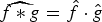 $\widehat{f \ast g} = \hat{f}\cdot \hat{g}$.
Lemma 5
Let f ∈ Lp, g ∈ Lq, where  $1 \leq p\comma \; q\comma \; r \leq \infty$ satisfy $1+\lpar {1}/{r}\rpar =\lpar {1}/{p}\rpar +\lpar {1}/{q}\rpar $. then
 $$\Vert f \ast g \Vert_r \leq \Vert f \Vert_p \Vert g \Vert_q.$$
Proof: The proof is based on the following inequalities [78, p. 174]
 $$\Vert f \ast g \Vert _1 \leq \Vert f\Vert_1 \Vert g\Vert_1\comma$$
 $$\Vert f \ast g \Vert_{\infty} \leq \Vert f\Vert_{\infty} \Vert g\Vert_1\comma$$
 $$\Vert f \ast g \Vert _{\infty} \leq \Vert f\Vert _p \Vert g\Vert _{p^{\prime}}\comma$$
where  $\lpar {1}/{p}\rpar +\lpar {1}/{p^{\prime}\rpar } = 1$. For a fixed function g ∈ L q, we define an operator ${\cal T}_g$ by $\lpar {\cal T}_{g}f\rpar \lpar n\rpar = \lpar f \ast g\rpar \lpar n\rpar $. Using (B.8) and (B.9), we observe that this operator is bounded from L 1 to L 1 by |g|1 and from L ∞ to L ∞ by |g|1. Thus, we can apply the Riesz–Thorin theorem to this operator to get
 $$\Vert f \ast g \Vert_p \leq \Vert f \Vert _p \Vert g \Vert _1.$$
 Similarly, for a fixed function f ∈ L p, we define another operator T f by  $\lpar T_{f}g\rpar \lpar n\rpar = \lpar f \ast g\rpar \lpar n\rpar $. From (B.11) and (B.10), we observe that this new operator is bounded from L 1 to L p by | f |p and from $L^{p^{\prime}}$ to L ∞ by | f |p. One more application of the Riesz–Thorin theorem leads to the desired result:
 $$\Vert f \ast g \Vert _r \leq \Vert f\Vert _p \Vert g\Vert_q\comma \;$$
where  $1+\lpar {1}/{r}\rpar =\lpar {1}/{p}\rpar +\lpar {1}/{q}\rpar $. □
Alternative proof of Theorem 3 for the case p ≥ 2: Suppose p > 2 and let  $\lpar {1}/{p}\rpar +\lpar {1}/{p^{\prime}\rpar }=1$. We denote the DFT by ${\cal F}$. Noting that $\lpar {p}/{p^{\prime}\rpar } \gt 1$, we have
 $$\eqalign{& \Vert {\cal A}_{{\cal D}_{DWFT}} f \Vert _p^p \cr &\quad = \sum_{u=1}^N \sum_{k=0}^{N-1} \vert {\cal A}_{{\cal D}_{DWFT}} f \lsqb u\comma \; k\rsqb \vert^p \cr &\quad= N^{{p}/{2}} \sum_{u=1}^N \sum_{k=0}^{N-1} \vert {\cal F} \lcub f\lsqb \cdot\rsqb g\lsqb u-\cdot\rsqb \rcub \lsqb k\rsqb \vert ^p \cr &\quad= N^{{p}/{2}} \sum_{u=1}^N \Vert {\cal F}\lcub f\lsqb \cdot\rsqb g\lsqb u-\cdot\rsqb \rcub \Vert _p^p \cr &\quad \leq N^{p/ 2} \sum_{u=1}^N N^{{p \over 2} - {p \over p^{\prime}}} \Vert f\lsqb \cdot\rsqb g\lsqb u-\cdot\rsqb \Vert _{p^{\prime}}^p \cr &\quad= N^{p-\lpar p/p^{\prime}\rpar } \sum_{u=1}^N \left(\sum_{n=1}^N \vert f\lsqb n\rsqb g\lsqb u-n\rsqb \vert^{p^{\prime}} \right)^{p/p^{\prime}}\cr &\quad = N^{p-\lpar p/p^{\prime}\rpar } \sum_{u=1}^N \left(\sum_{n=1}^N \vert f^{p^{\prime}}\lsqb n\rsqb \vert \vert g^{p^{\prime}}\lsqb u-n\rsqb \vert \right)^{p/p^{\prime}}}$$
 $$\eqalign{&\quad= N^{p-\lpar p/p^{\prime}\rpar } \sum_{u=1}^N \lpar \lpar \vert f^{p^{\prime}}\vert \ast \vert g^{p^{\prime}}\vert\rpar \lsqb u\rsqb \rpar ^{p/p^{\prime}} \cr &\quad= N^{p-\lpar p/p^{\prime}\rpar } \Vert \vert f^{p^{\prime}}\vert \ast \vert g^{p^{\prime}}\vert \Vert _{p/p^{\prime}}^{p/p^{\prime}} \cr &\quad \leq N^{p - \lpar p/p^{\prime}\rpar } \Vert f^{p^{\prime}} \Vert_{\alpha}^{p/p^{\prime}} \Vert g^{p^{\prime}} \Vert_{\beta}^{p/p^{\prime}} \cr &\quad=N \Vert f^{p^{\prime}} \Vert_{\alpha}^{p/p^{\prime}} \Vert g^{p^{\prime}}\Vert_{\beta}^{p/p^{\prime}}\comma \; }$$
for any  $1\leq \alpha\comma \; \beta \leq \infty$ satisfying $\lpar 1/\alpha\rpar + \lpar 1/\beta\rpar =p^{\prime}$. Equation (B.12) follows from the Hausdorff–Young inequality given in Lemma 4 and (B.13) follows from the Young inequality given in Lemma 5 with $r= p/p^{\prime}$. Now we can perform a change variable $a = \alpha p^{\prime}$ and $b = \beta p^{\prime}$ so that $\lpar 1/a\rpar +\lpar 1/b\rpar = 1$, and (B.13) becomes
 $$\Vert {\cal A}_{{\cal D}_{DWFT}} f \Vert_p^p \leq N \Vert f^{p^{\prime}}\Vert_{\alpha}^{p/p^{\prime}} \Vert g^{p^{\prime}} \Vert_\beta^{p/p^{\prime}} = N \Vert f\Vert_a^p \Vert g\Vert_b^p.$$
Finally, we take a = b = 2 and take the p th root of (B.14) to show the first half of Theorem 3. Note that we cannot follow the same line of logic for the case 1 ≤ p ≤ 2 without a converse of the Young's inequality in Lemma 5. □







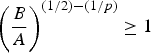


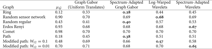


 Open access

