


1. Introduction
Linear logic (Girard 1987) can be viewed as a language of constructions in the operators
 \begin{equation*} \oplus , \otimes , \multimap , !\,. \end{equation*}
Most of these have meanings that are familiar from tensor algebra:
 $\oplus$
has the semantics of “direct sum,”
$\oplus$
has the semantics of “direct sum,”
 $\otimes$
is “tensor product” and
$\otimes$
is “tensor product” and
 $\multimap$
is “space of linear maps.” The exception is the exponential
$\multimap$
is “space of linear maps.” The exception is the exponential
 $!$
which has the semantics of a cofree coalgebra (Hyland and Schalk Reference Hyland and Schalk2003; Murfet 2014, 2015). The upshot is that linear logic gives a formal language for constructions in a canonical nonlinear extension of tensor algebra. While these operators are familiar to mathematicians, the fact that the structural maps associated to their universal properties can be used to encode algorithms is less familiar, and quite remarkable. This is a variant on the Curry–Howard–Lambek correspondence (Howard Reference Howard, Curry, Hindley, Seldin and Jonathan1980; Lambek and Scott Reference Lambek and Scott1988) and a consequence of the fact that proofs in intuitionistic linear logic can be interpreted as algorithms.
$!$
which has the semantics of a cofree coalgebra (Hyland and Schalk Reference Hyland and Schalk2003; Murfet 2014, 2015). The upshot is that linear logic gives a formal language for constructions in a canonical nonlinear extension of tensor algebra. While these operators are familiar to mathematicians, the fact that the structural maps associated to their universal properties can be used to encode algorithms is less familiar, and quite remarkable. This is a variant on the Curry–Howard–Lambek correspondence (Howard Reference Howard, Curry, Hindley, Seldin and Jonathan1980; Lambek and Scott Reference Lambek and Scott1988) and a consequence of the fact that proofs in intuitionistic linear logic can be interpreted as algorithms.
In particular, this means that we can translate algorithms into any category of mathematical objects where
 $\oplus , \otimes , \multimap , !$
can be interpreted. While the class of algorithms that can be encoded in (first-order, intuitionistic) linear logic is limited, it does include the execution of a Turing machine for a finite number of steps (Girard Reference Girard1994; Clift and Murfet Reference Clift and Murfet2020) and the interpretation of linear logic in vector spaces (Murfet 2015) has been used to make connections between Turing machines, the Ehrhard–Regnier derivative (Ehrhard and Regnier Reference Ehrhard and Regnier2003) and statistical learning theory (Clift and Murfet Reference Clift and Murfet2019; Clift et al. Reference Clift, Murfet and Wallbridge2021).
$\oplus , \otimes , \multimap , !$
can be interpreted. While the class of algorithms that can be encoded in (first-order, intuitionistic) linear logic is limited, it does include the execution of a Turing machine for a finite number of steps (Girard Reference Girard1994; Clift and Murfet Reference Clift and Murfet2020) and the interpretation of linear logic in vector spaces (Murfet 2015) has been used to make connections between Turing machines, the Ehrhard–Regnier derivative (Ehrhard and Regnier Reference Ehrhard and Regnier2003) and statistical learning theory (Clift and Murfet Reference Clift and Murfet2019; Clift et al. Reference Clift, Murfet and Wallbridge2021).
In this paper, we continue a project initiated in Murfet and Troiani (Reference Murfet and Troiani2022), which aims to find new interpretations of linear logic using algebraic geometry. At a conceptual level, the motivation is the simple idea that the structure of a proof lies in the pattern of repeated occurrences of some atomic degrees of freedom, which are somewhat implicit in sequent calculus or proof net presentations, but which are made explicit as “variables” in presentations like the lambda calculus (Murfet and Troiani 2020). We can think of such a pattern as constructed from a set of atoms
 $x,y,z,w,\ldots$
by a set of equations
$x,y,z,w,\ldots$
by a set of equations
 $x = y, y = z, z = w, \ldots$
and in that case, why not model these equations by an ideal
$x = y, y = z, z = w, \ldots$
and in that case, why not model these equations by an ideal
 $(x - y, y - z, z - w, \ldots )$
and then by a scheme? In this perspective, the role of sequents in a proof tree (or edges in a proof net) is to introduce the atomic degrees of freedom
$(x - y, y - z, z - w, \ldots )$
and then by a scheme? In this perspective, the role of sequents in a proof tree (or edges in a proof net) is to introduce the atomic degrees of freedom
 $x,y,z,w,\ldots$
and the role of deduction rules is to bind these atoms to each other by equations (Murfet and Troiani Reference Murfet and Troiani2022), which determine a geometric object.
$x,y,z,w,\ldots$
and the role of deduction rules is to bind these atoms to each other by equations (Murfet and Troiani Reference Murfet and Troiani2022), which determine a geometric object.
This idea is already mildly interesting in the case of multiplicative linear logic (MLL) proofs (those involving only
 $\otimes , \multimap$
) but the really interesting question is: what kind of equations, and thus geometry, represent the deduction rules in linear logic associated to the exponential?
$\otimes , \multimap$
) but the really interesting question is: what kind of equations, and thus geometry, represent the deduction rules in linear logic associated to the exponential?
In this paper, we give an answer to this question for a set of proof nets
 $\pi$
which we call shallow, for linear logic with the connectives
$\pi$
which we call shallow, for linear logic with the connectives
 $\otimes , \multimap , !$
(known as MELL), using the Hilbert scheme, which is the new ingredient necessary to interpret the exponential connective. To each shallow proof
$\otimes , \multimap , !$
(known as MELL), using the Hilbert scheme, which is the new ingredient necessary to interpret the exponential connective. To each shallow proof
 $\pi$
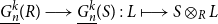
, we associate a closed immersion
$\pi$
, we associate a closed immersion
 \begin{equation} \mathbb{X}(\pi ) \longrightarrow \mathbb{S}(\pi ) \end{equation}
of schemes (Definition 3.0.6). Schemes are how we think about sets of solutions of polynomial equations in modern algebraic geometry. Here
 $\mathbb{S}(\pi )$
, which we refer to as the ambient scheme of
$\mathbb{S}(\pi )$
, which we refer to as the ambient scheme of
 $\pi$
, is a disjoint union of projective spaces
$\pi$
, is a disjoint union of projective spaces
 $\mathbb{P}^n_{\mathbb{k}}$
over the base field
$\mathbb{P}^n_{\mathbb{k}}$
over the base field
 $\mathbb{k}$
for various
$\mathbb{k}$
for various
 $n$
. The ambient scheme depends only on the formulas labelling the edges of the proof net (or equivalently the formulas appearing in sequents in the proof tree, if we think in terms of sequent calculus), whereas the full structure of
$n$
. The ambient scheme depends only on the formulas labelling the edges of the proof net (or equivalently the formulas appearing in sequents in the proof tree, if we think in terms of sequent calculus), whereas the full structure of
 $\pi$
is reflected in the closed subscheme
$\pi$
is reflected in the closed subscheme
 $\mathbb{X}(\pi )$
. As a closed subscheme of a locally projective scheme,
$\mathbb{X}(\pi )$
. As a closed subscheme of a locally projective scheme,
 $\mathbb{X}(\pi )$
is itself locally projective. In the conceptual picture introduced above,
$\mathbb{X}(\pi )$
is itself locally projective. In the conceptual picture introduced above,
 $\mathbb{S}(\pi )$
introduces the atomic degrees of freedom (the coordinates in the projective spaces) and
$\mathbb{S}(\pi )$
introduces the atomic degrees of freedom (the coordinates in the projective spaces) and
 $\mathbb{X}(\pi )$
says how the structure of
$\mathbb{X}(\pi )$
says how the structure of
 $\pi$
dictates that these degrees of freedom should be related to one another so that the geometry reflects the proof.
$\pi$
dictates that these degrees of freedom should be related to one another so that the geometry reflects the proof.
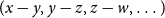
Our main theorem (Theorem3.1.3) says that the locally projective pair (1) is an invariant of proof nets, in the sense that we associate to any cut-reduction step
 $\gamma : \pi \longrightarrow \pi '$
a commutative diagram
$\gamma : \pi \longrightarrow \pi '$
a commutative diagram

in the category of schemes, where the bottom row is an isomorphism. This is the sense in which we mean that our construction is an interpretation of a (fragment of) linear logic. We expect that these ideas extend to arbitrary proof nets, but since this seems to require more sophisticated algebraic geometry, we feel it is worthwhile presenting the simple fragment separately (see Section 4).
While understanding the details about Hilbert schemes in this paper requires some nontrivial background in algebraic geometry, the geometry that is associated to the deduction rules involving exponentials is ultimately an expression of a simple idea. Promoting multiplicative proofs, which geometrically are interpreted by linear polynomials
 $x - y, y - z, z - w, \ldots$
, introduces additional atomic degrees of freedom
$x - y, y - z, z - w, \ldots$
, introduces additional atomic degrees of freedom
 $\theta , \phi , \psi , \ldots$
, which we can think of as parametrising a space of equations
$\theta , \phi , \psi , \ldots$
, which we can think of as parametrising a space of equations
 \begin{equation} x - \theta y - \phi z, \, y - \psi w - \kappa t, \ldots \end{equation}
in the sense that the point
 $\theta = 1, \phi = 0, \psi = 1, \kappa = 0$
in this parameter space stands for the system of equations
$\theta = 1, \phi = 0, \psi = 1, \kappa = 0$
in this parameter space stands for the system of equations
 $x = y, y = w$
, while the point
$x = y, y = w$
, while the point
 $\theta = 0, \phi = 1, \psi = 1, \kappa = 0$
stands for
$\theta = 0, \phi = 1, \psi = 1, \kappa = 0$
stands for
 $x = z, y = w$
. The deduction rules, like the contraction rule, which operate on exponentiated formulas, introduce equations between these parameters such as
$x = z, y = w$
. The deduction rules, like the contraction rule, which operate on exponentiated formulas, introduce equations between these parameters such as
 $\theta = \psi$
, which bind the identity of some equations to that of other equations (see Remark 3.2.1). In this way, our interpretation of shallow proof nets in locally projective pairs of schemes realises the exponential as having the semantics of a space of proofs and the geometric content of the deduction rules involving exponentiated formulas as equations between equations.
$\theta = \psi$
, which bind the identity of some equations to that of other equations (see Remark 3.2.1). In this way, our interpretation of shallow proof nets in locally projective pairs of schemes realises the exponential as having the semantics of a space of proofs and the geometric content of the deduction rules involving exponentiated formulas as equations between equations.
2. Shallow proofs and the Hilbert scheme
Proofs in MLL can be modelled by systems of linear equations between occurrences of formulas, and computation of a programme is in turn modelled by the elimination of variables appearing in these systems (Murfet and Troiani Reference Murfet and Troiani2022). This paper proves that shallow proofs (Definition 2.0.2) can be modelled by locally projective schemes. Algebraically, these locally projective schemes describe equations between formulas along with equations between these equations, as made precise in Remark 3.2.1.
Definition 2.0.1.
Let
 $A$
be a formula. We define the
depth of
$A$
be a formula. We define the
depth of
 $A$
,
$A$
,
 $\operatorname {Depth}(A)$
, by induction on the structure of
$\operatorname {Depth}(A)$
, by induction on the structure of
 $A$
as follows:
$A$
as follows:
-
• If
 $A$
is atomic, then
$\operatorname {Depth}(A) = 0$
.
$A$
is atomic, then
$\operatorname {Depth}(A) = 0$
. -
• If
$A = A_1 \boxtimes A_2$
, where
$\boxtimes \in \{\otimes , \unicode{x214B}\}$
, then
$\operatorname {Depth}(A) = \operatorname {max}\{\operatorname {Depth}(A_1), \operatorname {Depth}(A_2)\}$
. -
• If
$A = \neg A'$
, then
$\operatorname {Depth}(A) = \operatorname {Depth}(A')$
. -
• If
$A = \square A'$
, where
$\square \in \{!,?\}$
, then
$\operatorname {Depth}(A) = \operatorname {Depth}(A') + 1$
.


Definition 2.0.2.
A formula
 $A$
is
linear
if
$A$
is
linear
if
 $\operatorname {Depth}(A) = 0$
and is
shallow
if
$\operatorname {Depth}(A) = 0$
and is
shallow
if
 $\operatorname {Depth}(A) \leq 1$
. A proof
$\operatorname {Depth}(A) \leq 1$
. A proof
 $\pi$
is
linear
if all its formulas are.
$\pi$
is
linear
if all its formulas are.
Definition 2.0.3.
A proof
 $\pi$
is
pre-nearly linear
if the following hold:
$\pi$
is
pre-nearly linear
if the following hold:
-
• All conclusions to all Axiom-links are atomic.
-
• The conclusions of
$\pi$
are of the following form:
$?A_1, \ldots , ?A_n, B$
(where we allow for the possibility that
$n = 0$
), with
$A_1, \ldots , A_n, B$
linear.
-
• All edges of
$\pi$
are labelled by shallow formulas.
-
• There are no Weakening-links and there are no Promotion-links in
$\pi$
.


The
linear part
of a pre-nearly linear proof net
 $\pi$
is given by removing all Dereliction-links from
$\pi$
is given by removing all Dereliction-links from
 $\pi$
along with everything beneath these Dereliction-links and attaching the premises of these Dereliction-links to Conclusion-links.
$\pi$
along with everything beneath these Dereliction-links and attaching the premises of these Dereliction-links to Conclusion-links.
A proof net
 $\pi$
is
nearly linear
if it is pre-nearly linear and all persistent paths of the linear part of
$\pi$
is
nearly linear
if it is pre-nearly linear and all persistent paths of the linear part of
 $\pi$
go through
$\pi$
go through
 $B$
.
$B$
.
Definition 2.0.4. A proof is shallow if it satisfies the following:
-
• All of its edges are labelled by shallow formulas.
-
• There are no nested boxes.
-
• The interior of all boxes is nearly linear proof nets.
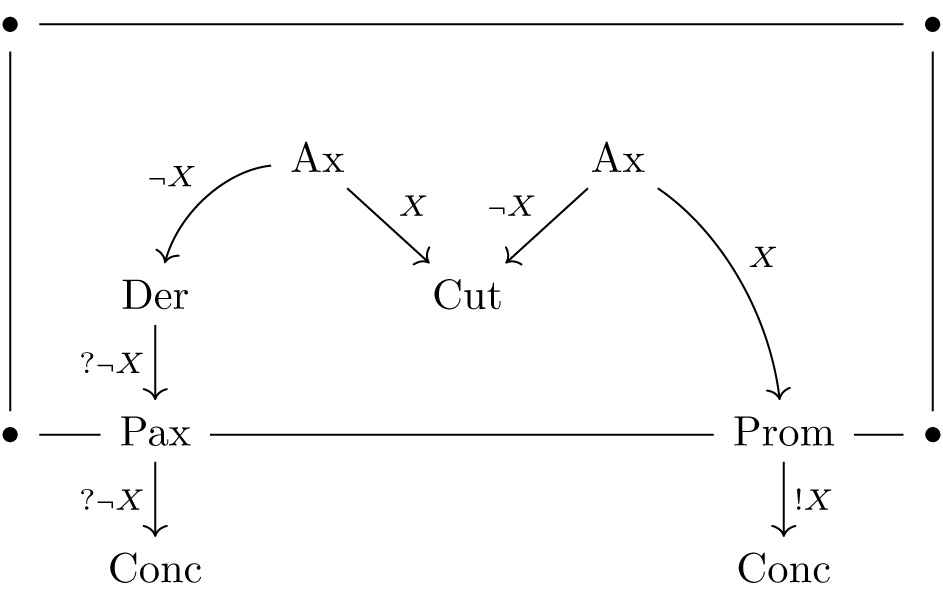
Example 2.0.5. Let
 $X$
be atomic. The following proof net is shallow:
$X$
be atomic. The following proof net is shallow:

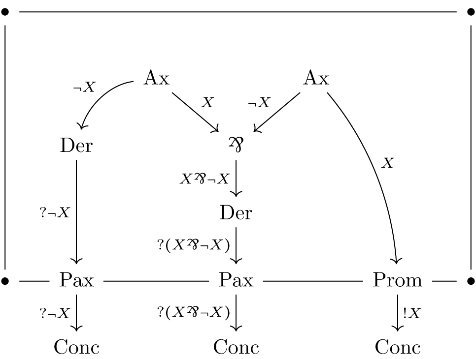
The following proof net is not shallow even though all of its formulas are:
It is cut-equivalent to the following proof net, which is shallow:
The following is not shallow because the linear part of the interior of the box fails to satisfy the property that all the persistent paths go through the premise of the Promotion-link:
Remark 2.0.6. The
 $\operatorname {Prom}/\operatorname {Pax}$
-reduction step involves nesting a box within another, and so necessarily involves proof nets which are not shallow. As a result, we do not consider this reduction step in this paper. In fact, it is possible to have a shallow proof net whose cut-elimination process necessarily involves a proof net which is not shallow (Example 4 is such a proof net). Thus, strong normalisation does not hold for the class of shallow proof nets. However, we do obtain normalisation for many algorithms of interest, for instance addition of Church numerals admits normalisation where all proof nets involved are shallow proof nets.
$\operatorname {Prom}/\operatorname {Pax}$
-reduction step involves nesting a box within another, and so necessarily involves proof nets which are not shallow. As a result, we do not consider this reduction step in this paper. In fact, it is possible to have a shallow proof net whose cut-elimination process necessarily involves a proof net which is not shallow (Example 4 is such a proof net). Thus, strong normalisation does not hold for the class of shallow proof nets. However, we do obtain normalisation for many algorithms of interest, for instance addition of Church numerals admits normalisation where all proof nets involved are shallow proof nets.
In Section 4, we give a research proposal for extending this model to all of MELL using a more general version of the Hilbert scheme.
2.1 The projective schemes associated to the algebraic model
In Murfet and Troiani (Reference Murfet and Troiani2022), we associated a coordinate ring
 $R_\pi$
to every MLL proof net
$R_\pi$
to every MLL proof net
 $\pi$
, defined as a quotient
$\pi$
, defined as a quotient
 $R_\pi = P_\pi /I_\pi$
, where
$R_\pi = P_\pi /I_\pi$
, where
 $P_\pi$
is a polynomial ring and
$P_\pi$
is a polynomial ring and
 $I_\pi$
is an ideal. While this algebraic construction is suitable for MLL proof nets, it is more natural to consider the associated schemes for shallow proofs. This shift in perspective is particularly helpful when working with the Hilbert scheme, as the Hilbert scheme lacks a straightforward algebraic counterpart.
$I_\pi$
is an ideal. While this algebraic construction is suitable for MLL proof nets, it is more natural to consider the associated schemes for shallow proofs. This shift in perspective is particularly helpful when working with the Hilbert scheme, as the Hilbert scheme lacks a straightforward algebraic counterpart.
In this section, we give an introduction to the Hilbert scheme, and in particular does not involve any novel content whatsoever.
2.2 The Hilbert functor
The construction of the Hilbert scheme begins with the Hilbert functor. Recall that for
 $R$
a ring,
$R$
a ring,
 $M$
an
$M$
an
 $R$
-module, and
$R$
-module, and
 $k \gt 0$
an integer,
$k \gt 0$
an integer,
 $M$
is locally free of rank
$M$
is locally free of rank
 $k$
if there exists
$k$
if there exists
 $n\gt 0$
and elements
$n\gt 0$
and elements
 $f_1, \ldots , f_n \in R$
such that for all
$f_1, \ldots , f_n \in R$
such that for all
 $i = 1 , \ldots , n$
,
$i = 1 , \ldots , n$
,
 $M_{f_i}$
is a free
$M_{f_i}$
is a free
 $R_{f_i}$
-module of rank
$R_{f_i}$
-module of rank
 $k$
. If
$k$
. If
 $T$
is a graded
$T$
is a graded
 $\mathbb{k}$
-algebra, and
$\mathbb{k}$
-algebra, and
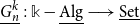
 $h: \mathbb{N} \longrightarrow \mathbb{N}$
is a function, then the Hilbert functor of
$h: \mathbb{N} \longrightarrow \mathbb{N}$
is a function, then the Hilbert functor of
 $T$
with respect to
$T$
with respect to
 $h$
is a functor
$h$
is a functor
 $\underline {H_T^h}: \mathbb{k}-\underline {\operatorname {Alg}} \longrightarrow \underline {\operatorname {Set}}$
, where
$\underline {H_T^h}: \mathbb{k}-\underline {\operatorname {Alg}} \longrightarrow \underline {\operatorname {Set}}$
, where
 $\underline {\operatorname {Set}}$
is the category of sets and functions. This functor maps a
$\underline {\operatorname {Set}}$
is the category of sets and functions. This functor maps a
 $\mathbb{k}$
-algebra
$\mathbb{k}$
-algebra
 $R$
to the following set, where
$R$
to the following set, where
 $R \otimes T$
denotes
$R \otimes T$
denotes
 $\bigoplus _{d \geq 0}R \otimes T_a$
:
$\bigoplus _{d \geq 0}R \otimes T_a$
:
 \begin{align*} \underline {H_T^h}(R) = \{I \subseteq R \otimes T &\mid I\text{ is homogeneous and } \forall d \geq 0,\\ &(R \otimes T_d)/I_d\text{ is a locally free }R\text{-module }\\ &\text{of rank }h(d)\}. \end{align*}
It was first proved by Grothendieck (Reference Grothendieck1961) that there exists a scheme
 $H_T^h$
representing this functor. That is, there is a natural isomorphism for each
$H_T^h$
representing this functor. That is, there is a natural isomorphism for each
 $R \in \mathbb{k}-\underline {\operatorname {Alg}}$
:
$R \in \mathbb{k}-\underline {\operatorname {Alg}}$
:
 \begin{equation} \underline {H_T^h}(R) \cong \operatorname {Hom}_{\underline {\operatorname {Sch}}_{\mathbb{k}}}\big(\!\operatorname {Spec}R, H_T^h\big) \end{equation}
where
 $\underline {\operatorname {Sch}}_{\mathbb{k}}$
is the category of schemes
$\underline {\operatorname {Sch}}_{\mathbb{k}}$
is the category of schemes
 $X \longrightarrow \operatorname {Spec}\mathbb{k}$
over
$X \longrightarrow \operatorname {Spec}\mathbb{k}$
over
 $\operatorname {Spec}\mathbb{k}$
and morphisms of schemes commuting over
$\operatorname {Spec}\mathbb{k}$
and morphisms of schemes commuting over
 $\operatorname {Spec}\mathbb{k}$
. We provide a detailed definition of this scheme in Section 2.3.2, and its construction has been reproduced in Troiani (Reference Troiani2024, Appendix D.6). This particular version of the Hilbert scheme along with its construction was first written down in Haiman and Sturmfels (Reference Haiman and Sturmfels2002).
$\operatorname {Spec}\mathbb{k}$
. We provide a detailed definition of this scheme in Section 2.3.2, and its construction has been reproduced in Troiani (Reference Troiani2024, Appendix D.6). This particular version of the Hilbert scheme along with its construction was first written down in Haiman and Sturmfels (Reference Haiman and Sturmfels2002).
2.3 Properties of the Hilbert scheme
Section 3 differs from the original Geometry of Interaction paper (Girard Reference Girard, Ferro, Bonotto, Valentini and Zanardo1989), where rather than interpreting exponentials using the Hilbert scheme, Girard interpreted exponentials using the Hilbert hotel. To understand the geometry of our model, one need not first acquire a knowledge of the Hilbert scheme’s construction, but one must understand some of its properties. We have organised this paper so that the minimal theory of the Hilbert scheme required to understand our model is presented, and then the algebraic geometry involving the construction of the Hilbert scheme can be found in Troiani (Reference Troiani2024).
2.3.1 The Grassmann scheme
Definition 2.3.1.
Let
 $X$
be a scheme. We denote the following functor by
$X$
be a scheme. We denote the following functor by
 $h_X$
, which acts on objects as
$h_X$
, which acts on objects as
 \begin{align*} h_X: \mathbb{k}-\underline {\operatorname {Alg}} &\longrightarrow \underline {\operatorname {Set}}\\ R &\longmapsto \operatorname {Hom}_{\underline {\operatorname {Sch}}_{\mathbb{k}}}(\!\operatorname {Spec}R, X) \end{align*}
and which maps a homomorphism of
 $\mathbb{k}$
-algebras
$\mathbb{k}$
-algebras
 $f: R \longrightarrow T$
to the composition map
$f: R \longrightarrow T$
to the composition map
 \begin{align*} \hat {f} \circ ({-}): \operatorname {Hom}(\!\operatorname {Spec}R, X) &\longrightarrow \operatorname {Hom}(\!\operatorname {Spec}T, X)\\ g &\longmapsto \hat {f} \circ g \end{align*}
where
 $\hat {f}: \operatorname {Spec}T \longrightarrow \operatorname {Spec}R$
is induced by
$\hat {f}: \operatorname {Spec}T \longrightarrow \operatorname {Spec}R$
is induced by
 $f$
.
$f$
.
Definition 2.3.2.
If
 $F: \mathbb{k}-\underline {\operatorname {Alg}} \longrightarrow \underline {\operatorname {Set}}$
is a functor and there exists a scheme
$F: \mathbb{k}-\underline {\operatorname {Alg}} \longrightarrow \underline {\operatorname {Set}}$
is a functor and there exists a scheme
 $X$
such that
$X$
such that
 $F \cong h_X$
, then
$F \cong h_X$
, then
 $F$
is
representable
and is
represented
by
$F$
is
representable
and is
represented
by
 $X$
.
$X$
.
Let
 $R$
be a
$R$
be a
 $\mathbb{k}$
-algebra. Let
$\mathbb{k}$
-algebra. Let
 $n \gt 0$
,
$n \gt 0$
,
 $0 \lt k \lt n$
, and define the following set:
$0 \lt k \lt n$
, and define the following set:
 \begin{align*} \underline {G_n^k}(R) = \{ L \subseteq R^n &\mid L\text{ is an }R\text{ submodule, and }\\ &R^n/L\text{ is a locally free }R\text{-module of rank }k\}. \end{align*}
Given an element
 $L \in \underline {G_n^k}(R)$
and a
$L \in \underline {G_n^k}(R)$
and a
 $\mathbb{k}$
-algebra homomorphism
$\mathbb{k}$
-algebra homomorphism
 $\phi : R \longrightarrow S$
, we can tensor the short exact sequence
$\phi : R \longrightarrow S$
, we can tensor the short exact sequence

by
 $S$
over
$S$
over
 $R$
and obtain a new short exact sequence, which is isomorphic to the following:
$R$
and obtain a new short exact sequence, which is isomorphic to the following:
It follows that
 $S^n/(S \otimes _{\mathbb{k}}L)$
is locally free of rank
$S^n/(S \otimes _{\mathbb{k}}L)$
is locally free of rank
 $k$
if
$k$
if
 $R^n/L$
is. Thus we have a well defined map
$R^n/L$
is. Thus we have a well defined map
 $\underline {G_n^k}(R) \longrightarrow \underline {G_n^k}(S): L \longmapsto S \otimes _R L$
, which is denoted
$\underline {G_n^k}(R) \longrightarrow \underline {G_n^k}(S): L \longmapsto S \otimes _R L$
, which is denoted
 $\underline {G_n^k}(\phi )$
. This extends
$\underline {G_n^k}(\phi )$
. This extends
 $\underline {G_n^k}$
to a functor.
$\underline {G_n^k}$
to a functor.
Definition 2.3.3.
The functor
 $\underline {G_n^k}: \mathbb{k}-\underline {\operatorname {Alg}} \longrightarrow \underline {\operatorname {Set}}$
is the
Grassmann Functor
.
$\underline {G_n^k}: \mathbb{k}-\underline {\operatorname {Alg}} \longrightarrow \underline {\operatorname {Set}}$
is the
Grassmann Functor
.
Example 2.3.4. Consider the
 $\mathbb{C}$
-algebra
$\mathbb{C}$
-algebra
 $\mathbb{C}^2$
. Then, for any
$\mathbb{C}^2$
. Then, for any
 $\mathbb{C}$
-algebra
$\mathbb{C}$
-algebra
 $R$
, we have
$R$
, we have
 $R \otimes _{\mathbb{C}}\mathbb{C}^2 \cong R^2$
. Let
$R \otimes _{\mathbb{C}}\mathbb{C}^2 \cong R^2$
. Let
 $e_1, e_2$
be the standard
$e_1, e_2$
be the standard
 $R$
-basis for
$R$
-basis for
 $R^2$
and consider a short exact sequence
$R^2$
and consider a short exact sequence

then
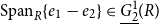 $\operatorname {Span}_R\{e_1 - e_2\} \in \underline {G_2^1}(R)$
.
$\operatorname {Span}_R\{e_1 - e_2\} \in \underline {G_2^1}(R)$
.
Let
 $\{ e_1, \ldots , e_n \}$
be the standard basis vectors for
$\{ e_1, \ldots , e_n \}$
be the standard basis vectors for
 $R^n$
and
$R^n$
and
 $B = \{e_{i_1}, \ldots , e_{i_k}\} \subseteq \{ e_1, \ldots , e_n \}$
be a size
$B = \{e_{i_1}, \ldots , e_{i_k}\} \subseteq \{ e_1, \ldots , e_n \}$
be a size
 $k$
subset with
$k$
subset with
 $i_1 \lt \ldots \lt i_k$
. Among the elements of
$i_1 \lt \ldots \lt i_k$
. Among the elements of
 $\underline {G_n^k}(R)$
are the modules
$\underline {G_n^k}(R)$
are the modules
 $L \in \underline {G_n^k}(R)$
such that
$L \in \underline {G_n^k}(R)$
such that
 $R^n/L$
has basis
$R^n/L$
has basis
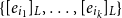 $\{ [e_{i_1}]_L, \ldots , [e_{i_k}]_L \}$
, where for
$\{ [e_{i_1}]_L, \ldots , [e_{i_k}]_L \}$
, where for
 $i_1, \ldots , i_k$
the notation
$i_1, \ldots , i_k$
the notation
 $[e_{i_j}]_L$
denotes the image of
$[e_{i_j}]_L$
denotes the image of
 $e_i \in R^n$
under the standard quotient map
$e_i \in R^n$
under the standard quotient map
 $R^n \longrightarrow R^n/L$
. We will denote by
$R^n \longrightarrow R^n/L$
. We will denote by
 $[B]_{L}$
the set
$[B]_{L}$
the set
 $\{ [e_{i_1}]_L, \ldots , [e_{i_k}]_L \}$
.
$\{ [e_{i_1}]_L, \ldots , [e_{i_k}]_L \}$
.
Definition 2.3.5. Define the following subset
 \begin{equation} \underline {G^k_{n\backslash B}}(R) := \{ L \in \underline {G^k_n}(R) \mid R^n/L\text{ is free with }R\text{-basis }[B]_L \} \subseteq \underline {G^k_n}(R). \end{equation}
This extends to a full subfunctor of
 $\underline {G_n^k}$
.
$\underline {G_n^k}$
.
Lemma 2.3.6.
The functor
 $\underline {G^k_{n\backslash B}}$
is represented by
$\underline {G^k_{n\backslash B}}$
is represented by
 \begin{equation} \operatorname {Spec}\mathbb{k}\left[\left\{z_i^j \mid 1 \leq i \leq k, 1 \leq j \leq n - k\right\}\right]. \end{equation}
Proof.
Fix a
 $\mathbb{k}$
-algebra
$\mathbb{k}$
-algebra
 $R$
. If
$R$
. If
 $L \in \underline {G_{n\backslash B}^k}$
, then for each
$L \in \underline {G_{n\backslash B}^k}$
, then for each
 $e_{m} \not \in B$
we have
$e_{m} \not \in B$
we have
 \begin{equation} [e_{m}] = \sum _{i = 1}^k \alpha _{i}^j[e_{i_j}] \end{equation}
for some coefficients
 $\{\alpha _{i}^j\}_{1 \leq i \leq k, 1 \leq j \leq n-k} \subseteq R$
. The data of these coefficients are equivalent to the data of a
$\{\alpha _{i}^j\}_{1 \leq i \leq k, 1 \leq j \leq n-k} \subseteq R$
. The data of these coefficients are equivalent to the data of a
 $\mathbb{k}$
-algebra morphism
$\mathbb{k}$
-algebra morphism
 \begin{equation} \mathbb{k}\big[\big\{z_i^j\big\}\big] \longrightarrow R \end{equation}
which in turn is equivalent to the data of a morphism
 $\operatorname {Spec}R \longrightarrow \operatorname {Spec}\mathbb{k}[\{z_i^j\}]$
.
$\operatorname {Spec}R \longrightarrow \operatorname {Spec}\mathbb{k}[\{z_i^j\}]$
.
Proposition 2.3.7.
For all
 $n \gt k \gt 0$
, the functor
$n \gt k \gt 0$
, the functor
 $\underline {G_n^k}$
is represented by a closed subscheme of
$\underline {G_n^k}$
is represented by a closed subscheme of
 $\mathbb{P}^{\binom {n}{k}-1}$
.
$\mathbb{P}^{\binom {n}{k}-1}$
.
Proof.
The representing scheme can be constructed by gluing together the schemes 8 ranging over all
 $B$
, see Troiani (Reference Troiani2024, Appendix D.5).
$B$
, see Troiani (Reference Troiani2024, Appendix D.5).
Definition 2.3.8.
We denote the projective scheme representing the functor
 $\underline {G_n^k}$
by
$\underline {G_n^k}$
by
 $G_n^k$
. This is the
Grassmann scheme
.
$G_n^k$
. This is the
Grassmann scheme
.
2.3.2 The Hilbert scheme
We follow Haiman and Sturmfels (Reference Haiman and Sturmfels2002).
Definition 2.3.9.
A
graded
 $\mathbb{k}$
-module with operators
is a pair
$\mathbb{k}$
-module with operators
is a pair
 $(T,F)$
consisting of a graded
$(T,F)$
consisting of a graded
 $\mathbb{k}$
-module
$\mathbb{k}$
-module
 \begin{equation} T = \bigoplus _{d \in \mathbb{N}}T_d \end{equation}
and a family of operators
 \begin{equation} F = \bigcup _{d,e \in \mathbb{N}}F_{d,e} \end{equation}
where for all
 $d,e \in \mathbb{N}, F_{d,e} \subseteq \operatorname {Hom}(T_d, T_e)$
.
$d,e \in \mathbb{N}, F_{d,e} \subseteq \operatorname {Hom}(T_d, T_e)$
.
Definition 2.3.10.
Let
 $(T,F)$
be a graded
$(T,F)$
be a graded
 $\mathbb{k}$
-module with operators. A graded submodule
$\mathbb{k}$
-module with operators. A graded submodule
 \begin{equation} L = \bigoplus _{d \in \mathbb{N}}L_d \subseteq T \end{equation}
is an
 $F$
-submodule
if
$F$
-submodule
if
 $F_{d,e}(L_d) \subseteq L_e$
for all
$F_{d,e}(L_d) \subseteq L_e$
for all
 $d, e \in \mathbb{N}$
.
$d, e \in \mathbb{N}$
.
Example 2.3.11. If
 $T$
is a graded
$T$
is a graded
 $\mathbb{k}$
-algebra, then for
$\mathbb{k}$
-algebra, then for
 $a,b \in \mathbb{N}$
, define:
$a,b \in \mathbb{N}$
, define:
 \begin{equation} F_{a,b} = \begin{cases} \text{The set of multiplications by monomials of degree }e - d,& d \geq e\\ \varnothing ,&d\lt e \end{cases} \end{equation}
then any homogeneous ideal is a homogeneous
 $F$
-module, where
$F$
-module, where
 $F = \{F_{d,e}\}_{d,e \in \mathbb{N}}$
.
$F = \{F_{d,e}\}_{d,e \in \mathbb{N}}$
.
Definition 2.3.12.
If
 $(T,F)$
is a graded
$(T,F)$
is a graded
 $\mathbb{k}$
-module with operators and
$\mathbb{k}$
-module with operators and
 $D \subseteq \mathbb{N}$
is a subset of the degrees, we denote by
$D \subseteq \mathbb{N}$
is a subset of the degrees, we denote by
 $(T_D, F_D)$
the graded
$(T_D, F_D)$
the graded
 $\mathbb{k}$
-module with operators, where
$\mathbb{k}$
-module with operators, where
 \begin{equation} T_D = \bigoplus _{d \in D}T_d,\quad F_D = \{F_{d,e} \in F\mid d,e \in D\operatorname \}. \end{equation}
Let
 $R$
be a commutative
$R$
be a commutative
 $\mathbb{k}$
-algebra. Notice that if
$\mathbb{k}$
-algebra. Notice that if
 $(T,F)$
is a graded
$(T,F)$
is a graded
 $\mathbb{k}$
-module with operators, then so is
$\mathbb{k}$
-module with operators, then so is
 \begin{equation} R \otimes T := \bigoplus _{d \in \mathbb{N}}R \otimes T_d \end{equation}
when paired with the operators
 $\hat {F} = \{\operatorname {id}_R \otimes F_{d,e}\}_{d,e \in \mathbb{N}}$
. Given a function
$\hat {F} = \{\operatorname {id}_R \otimes F_{d,e}\}_{d,e \in \mathbb{N}}$
. Given a function
 $h: \mathbb{N} \longrightarrow \mathbb{N}$
, we define the set
$h: \mathbb{N} \longrightarrow \mathbb{N}$
, we define the set
 \begin{align*} \underline {H_T^h}(R) = \{ F-\text{submodules } L \subseteq R \otimes T &\mid \forall d \in \mathbb{N}, (R \otimes T_d)/L_d\text{ is }\\ &\text{ locally free of rank }h(d)\}. \end{align*}
Let
 $\phi : R \longrightarrow S$
be a
$\phi : R \longrightarrow S$
be a
 $\mathbb{k}$
-algebra homomorphism and let
$\mathbb{k}$
-algebra homomorphism and let
 $f_1, \ldots , f_n \in R$
be a set of elements generating the unit ideal. Then for any
$f_1, \ldots , f_n \in R$
be a set of elements generating the unit ideal. Then for any
 $d \in \mathbb{N}$
and any
$d \in \mathbb{N}$
and any
 $i = 1, \ldots , n$
, there is a short exact sequence
$i = 1, \ldots , n$
, there is a short exact sequence
By tensoring with
 $S$
over
$S$
over
 $R$
, we obtain a similar short exact sequence. The function
$R$
, we obtain a similar short exact sequence. The function
 $\underline {H_T^h}(R) \longrightarrow \underline {H_T^h}(S), L \longrightarrow S \otimes L$
is denoted
$\underline {H_T^h}(R) \longrightarrow \underline {H_T^h}(S), L \longrightarrow S \otimes L$
is denoted
 $\underline {H_T^h}(\phi )$
. It is easy to see that
$\underline {H_T^h}(\phi )$
. It is easy to see that
 $\underline {H_T^h}: \mathbb{k}-\underline {\operatorname {Alg}} \longrightarrow \underline {\operatorname {Set}}$
is a functor.
$\underline {H_T^h}: \mathbb{k}-\underline {\operatorname {Alg}} \longrightarrow \underline {\operatorname {Set}}$
is a functor.
Definition 2.3.13.
The functor
 $\underline {H_T^h}$
is the
Hilbert functor
.
$\underline {H_T^h}$
is the
Hilbert functor
.
Definition 2.3.14.
Let
 $D \subseteq \mathbb{N}$
. The
restriction
is the following natural transformation
$D \subseteq \mathbb{N}$
. The
restriction
is the following natural transformation
 $\operatorname {Res}_{T_D}: \underline {H_T^h} \longrightarrow \underline {H_{T_D}^h}$
which maps an element
$\operatorname {Res}_{T_D}: \underline {H_T^h} \longrightarrow \underline {H_{T_D}^h}$
which maps an element
 $L \in \underline {H_T^h}(R)$
to the restriction
$L \in \underline {H_T^h}(R)$
to the restriction
 $L_D = \bigoplus _{d \in D}L_d$
.
$L_D = \bigoplus _{d \in D}L_d$
.
Theorem 2.3.15.
Let
 $(T,F)$
be a graded
$(T,F)$
be a graded
 $\mathbb{k}$
-module with operators. Let
$\mathbb{k}$
-module with operators. Let
 $h: \mathbb{N} \longrightarrow \mathbb{N}$
be a function such that
$h: \mathbb{N} \longrightarrow \mathbb{N}$
be a function such that
 $\sum _{d \in \mathbb{N}}h(d) \lt \infty$
. Suppose
$\sum _{d \in \mathbb{N}}h(d) \lt \infty$
. Suppose
 $M \subseteq N \subseteq T$
are homogeneous
$M \subseteq N \subseteq T$
are homogeneous
 $\mathbb{k}$
-submodules satisfying:
$\mathbb{k}$
-submodules satisfying:
-
•
$N$
is a finitely generated
$\mathbb{k}$
-module.
-
•
$N$
generates
$T$
as an
$F$
-module.
-
• For every field
$K \in \mathbb{k}-\underline {\operatorname {Alg}}$
and every
$L \in \underline {H_T^h(K)}$
,
$M$
generates
$(K \otimes T)/L$
as a
$K$
-module.
-
• There is a subset
$G \subseteq F$
so that
$G$
is the closure of
$F$
under composition and
$G$
is such that
$GM \subseteq N$
.


Then
 $\underline {H_T^h}$
is represented by a quasiprojective scheme
$\underline {H_T^h}$
is represented by a quasiprojective scheme
 $H_T^h$
.
$H_T^h$
.
Proof. See Haiman and Sturmfels (Reference Haiman and Sturmfels2002, Theorem 2.2). We also reproduced this proof in Troiani (Reference Troiani2024, Section D.6).
Theorem2.3.15 only holds when
 $h$
is such that
$h$
is such that
 $\sum _{d \in \mathbb{N}}h(d) \lt \infty$
because we construct
$\sum _{d \in \mathbb{N}}h(d) \lt \infty$
because we construct
 $H_T^h$
as a subscheme of
$H_T^h$
as a subscheme of
 $G^r_n$
for some
$G^r_n$
for some
 $r \gt \sum _{d \in \mathbb{N}}h(d)$
. We wish to apply Theorem2.3.15 in the setting where
$r \gt \sum _{d \in \mathbb{N}}h(d)$
. We wish to apply Theorem2.3.15 in the setting where
 $h$
is the Hilbert function (recalled in Definition 2.3.16) of a homogeneous ideal of
$h$
is the Hilbert function (recalled in Definition 2.3.16) of a homogeneous ideal of
 $\mathbb{k}[x_0, \ldots , x_n]$
(given with respect to the standard grading). This function in general is not of finite support. To mitigate this, we follow Haiman and Sturmfels (Reference Haiman and Sturmfels2002) and construct a subset
$\mathbb{k}[x_0, \ldots , x_n]$
(given with respect to the standard grading). This function in general is not of finite support. To mitigate this, we follow Haiman and Sturmfels (Reference Haiman and Sturmfels2002) and construct a subset
 $D \subseteq \mathbb{N}$
to exhibit the Hilbert functor
$D \subseteq \mathbb{N}$
to exhibit the Hilbert functor
 $\underline {H_T^h}$
as a subfunctor of
$\underline {H_T^h}$
as a subfunctor of
 $\underline {H_{T_D}^h}$
. We then relate to this a closed immersion of schemes
$\underline {H_{T_D}^h}$
. We then relate to this a closed immersion of schemes
 $H_T^h \longrightarrow H_{T_D}^h$
.
$H_T^h \longrightarrow H_{T_D}^h$
.
Definition 2.3.16.
Let
 $S$
be a graded
$S$
be a graded
 $\mathbb{k}$
-algebra and
$\mathbb{k}$
-algebra and
 $I \subseteq S$
a homogeneous ideal. The
Hilbert function
of
$I \subseteq S$
a homogeneous ideal. The
Hilbert function
of
 $I$
is the function
$I$
is the function
 \begin{align*} \mathbb{N} &\longrightarrow \mathbb{N}\\ n &\longmapsto \operatorname {dim}_{\mathbb{k}}(S_n/I_n). \end{align*}
Proposition 2.3.17.
Let
 $d \gt 0, c \gt 0$
. There exists a unique expression
$d \gt 0, c \gt 0$
. There exists a unique expression
 \begin{equation} c = \binom {k_d}{d} + \binom {k_{d-1}}{d-1} + \cdots + \binom {k_\delta }{\delta } \end{equation}
where
 $k_d \gt k_{d-1} \gt \cdots \gt k_\delta \geq \delta \gt 0$
.
$k_d \gt k_{d-1} \gt \cdots \gt k_\delta \geq \delta \gt 0$
.
Proof.
We proceed by induction on
 $c$
.
$c$
.
Say
 $c = 1$
. Then for any
$c = 1$
. Then for any
 $d \gt 0$
 \begin{equation} 1 = \binom {d}{d}. \end{equation}
Since for all
 $a\gt d$
we have
$a\gt d$
we have
 $\binom {a}{d} \gt 1$
, it is clear that (19) is the unique such expression.
$\binom {a}{d} \gt 1$
, it is clear that (19) is the unique such expression.
Say
 $c \gt 1$
. First, we prove existence of such an expression. Let
$c \gt 1$
. First, we prove existence of such an expression. Let
 $k_d$
denote the largest integer such that
$k_d$
denote the largest integer such that
 \begin{equation} c \geq \binom {k_d}{d}. \end{equation}
If (20) holds to equality, then we are done, so assume
 $c - \binom {k_d}{d} \gt 0$
which by the inductive hypothesis implies there exists unique
$c - \binom {k_d}{d} \gt 0$
which by the inductive hypothesis implies there exists unique
 $k_{d-1} \gt \cdots \gt k_{\delta } \gt 0$
such that
$k_{d-1} \gt \cdots \gt k_{\delta } \gt 0$
such that
 \begin{equation} c - \binom {k_d}{d} = \binom {k_{d-1}}{d-1} + \cdots + \binom {k_{\delta }}{\delta }. \end{equation}
We must show that
 $k_d \gt k_{d-1}$
. Suppose to the contrary that
$k_d \gt k_{d-1}$
. Suppose to the contrary that
 $k_d \leq k_{d-1}$
. Then
$k_d \leq k_{d-1}$
. Then
 \begin{equation} \binom {k_d}{d-1} \leq \binom {k_{d-1}}{d-1} \end{equation}
and so, using (21), we have
 \begin{equation} c \geq \binom {k_{d-1}}{d-1} + \binom {k_d}{d} \geq \binom {k_{d}}{d-1} + \binom {k_d}{d} = \binom {k_{d}+1}{d} \end{equation}
which contradicts maximality of
 $k_d$
.
$k_d$
.
Now we prove uniqueness. Assume there were two expressions:
 \begin{align*} c &= \binom {k_d}{d} + \binom {k_{d-1}}{d-1} + \cdots + \binom {k_\delta }{\delta }\\ c &= \binom {k_d'}{d} + \binom {k_{d-1}'}{d-1} + \cdots + \binom {k_{\delta '}'}{\delta '} \end{align*}
with
 $k_d \gt k_{d-1} \gt \cdots \gt k_\delta \gt 0, k_d' \gt k_{d-1}' \gt \cdots \gt k_{\delta '}' \gt 0$
. Let
$k_d \gt k_{d-1} \gt \cdots \gt k_\delta \gt 0, k_d' \gt k_{d-1}' \gt \cdots \gt k_{\delta '}' \gt 0$
. Let
 $s \leq d$
be the greatest integer such that
$s \leq d$
be the greatest integer such that
 $k_s \neq k_s'$
. By considering
$k_s \neq k_s'$
. By considering
 $c - \sum _{i = s}^d \binom {k_{i}}{i}$
in place of
$c - \sum _{i = s}^d \binom {k_{i}}{i}$
in place of
 $c$
, we may assume
$c$
, we may assume
 $s = d$
.
$s = d$
.
Assume without loss of generality that
 $k_d' \lt k_d$
. Since
$k_d' \lt k_d$
. Since
 $k_d'$
is an integer, we have
$k_d'$
is an integer, we have
 $k_d' \leq k_d - 1$
. By the inductive hypothesis, the expression
$k_d' \leq k_d - 1$
. By the inductive hypothesis, the expression
 \begin{equation} c - \binom {k_d'}{d} = \binom {k_{d-1}'}{d-1} + \cdots + \binom {k_{\delta '}'}{\delta '} \end{equation}
is the unique such, and so
 $k_{d-1}'$
is the maximal integer such that
$k_{d-1}'$
is the maximal integer such that
 \begin{equation} c - \binom {k_d'}{d} \geq \binom {k_{d-1}'}{d-1}. \end{equation}
Since
 $k_d \gt k_d'$
, we have:
$k_d \gt k_d'$
, we have:
 \begin{equation} c - \binom {k_d'}{d} \gt c - \binom {k_d}{d} = \binom {k_{d}-1}{d-1} + \cdots + \binom {k_\delta }{\delta } \geq \binom {k_d-1}{d-1} \end{equation}
and so
 $k_d - 1 \leq k_{d-1}'$
. Thus,
$k_d - 1 \leq k_{d-1}'$
. Thus,
 $k_d' \leq k_{d-1}'$
, which is a contradiction.
$k_d' \leq k_{d-1}'$
, which is a contradiction.
Definition 2.3.18.
The
 $d$
-binomial expansion of
$d$
-binomial expansion of
 $c$
is the unique expansion given by (
18
). The
$c$
is the unique expansion given by (
18
). The
 $d^{\text{th}}$
Macaulay difference set of
$d^{\text{th}}$
Macaulay difference set of
 $c$
,
$c$
,
 $M_d(c)$
is defined as the tuple
$M_d(c)$
is defined as the tuple
 \begin{equation} M_d(c) = (k_d - d, d_{d-1} - (d-1), \ldots , k_\delta - \delta ). \end{equation}
We note that the data of the
 $d$
-binomial expansion of
$d$
-binomial expansion of
 $c$
are equivalent to that of the
$c$
are equivalent to that of the
 $d^{\text{th}}$
Macaulay difference set of
$d^{\text{th}}$
Macaulay difference set of
 $c$
.
$c$
.
Example 2.3.19. The following is the 4-binomial expansion of
 $27$
:
$27$
:
 \begin{equation} 27 = \binom {6}{4} + \binom {5}{3} + \binom {2}{2} + \binom {1}{1}. \end{equation}
The
 $4^{\text{th}}$
Macaulay difference set of 27 is
$4^{\text{th}}$
Macaulay difference set of 27 is
 $(2,2,0,0)$
.
$(2,2,0,0)$
.
Definition 2.3.20.
Let
 $c \gt 0, d \gt 0$
, and let
$c \gt 0, d \gt 0$
, and let
 $k_d \gt k_{d-1} \gt \cdots \gt k_\delta \geq \delta \gt 0$
be the integers involved in the
$k_d \gt k_{d-1} \gt \cdots \gt k_\delta \geq \delta \gt 0$
be the integers involved in the
 $d$
-binomial expansion of
$d$
-binomial expansion of
 $c$
as in Proposition 2.3.17
. Define the following natural number:
$c$
as in Proposition 2.3.17
. Define the following natural number:
 \begin{equation} c^{\langle d \rangle } = \binom {k_d + 1}{d+ 1} + \binom {k_{d-1} + 1}{d} + \cdots + \binom {k_{\delta } + 1}{\delta + 1}. \end{equation}
Remark 2.3.21. The
 $d^{\text{th}}$
Macaulay difference set of
$d^{\text{th}}$
Macaulay difference set of
 $c$
and the
$c$
and the
 $(d+1)^{\text{th}}$
Macaulay difference set of
$(d+1)^{\text{th}}$
Macaulay difference set of
 $c^{\langle d \rangle }$
are equal.
$c^{\langle d \rangle }$
are equal.
Proposition 2.3.22.
Fix
 $n \gt 0$
and a homogeneous ideal
$n \gt 0$
and a homogeneous ideal
 $I \subseteq \mathbb{k}[x_0, \ldots , x_n]$
. Let
$I \subseteq \mathbb{k}[x_0, \ldots , x_n]$
. Let
 $h$
be the Hilbert function of
$h$
be the Hilbert function of
 $I$
. There exists an integer
$I$
. There exists an integer
 $j$
such that for all
$j$
such that for all
 $d \geq j$
we have
$d \geq j$
we have
 \begin{equation} h(d+1) = h(d)^{\langle d \rangle }. \end{equation}
Proof. See Ahn et al. (Reference Ahn, Geramita and Shin2009, Section 2).
Corollary 2.3.23.
Let
 $I \subseteq \mathbb{k}[x_0, \ldots , x_n]$
be homogeneous with Hilbert function
$I \subseteq \mathbb{k}[x_0, \ldots , x_n]$
be homogeneous with Hilbert function
 $h$
. Let
$h$
. Let
 $j$
be the integer such that for all
$j$
be the integer such that for all
 $d \geq j$
we have (
30
). Then for all
$d \geq j$
we have (
30
). Then for all
 $d \geq j$
, the
$d \geq j$
, the
 $d^{\text{th}}$
Macaulay difference set of
$d^{\text{th}}$
Macaulay difference set of
 $h(d)$
is equal to the
$h(d)$
is equal to the
 $j^{\text{th}}$
Macaulay difference set of
$j^{\text{th}}$
Macaulay difference set of
 $h(j)$
.
$h(j)$
.
Proof.
For
 $d \geq j$
, we have
$d \geq j$
, we have
 \begin{equation} M_{d+1}(h(d+1)) = M_{d+1}(h(d)^{\langle d \rangle }) = M_{d}(h(d)) \end{equation}
where the first equality holds by Proposition 2.3.22 and the second by Remark 2.3.21.
Definition 2.3.24.
Let
 $I \subseteq \mathbb{k}[x_0, \ldots , x_n]$
be a homogeneous ideal. The
Gotzmann number
$I \subseteq \mathbb{k}[x_0, \ldots , x_n]$
be a homogeneous ideal. The
Gotzmann number
 $G(I)$
of
$G(I)$
of
 $I \subseteq \mathbb{k}[x_0, \ldots , x_n]$
is the number of elements in the eventually constant
$I \subseteq \mathbb{k}[x_0, \ldots , x_n]$
is the number of elements in the eventually constant
 $d^{\text{th}}$
Macaulay difference set of
$d^{\text{th}}$
Macaulay difference set of
 $h(d)$
.
$h(d)$
.
Example 2.3.25. Consider the Segre embedding (see Corollary (Troiani Reference Troiani2024, Corollary 3.7) for a reminder)
 $\operatorname {Seg}: \mathbb{P}^1 \times \mathbb{P}^1 \longrightarrow \mathbb{P}^3$
and the canonical closed immersion of the diagonal
$\operatorname {Seg}: \mathbb{P}^1 \times \mathbb{P}^1 \longrightarrow \mathbb{P}^3$
and the canonical closed immersion of the diagonal
 $\iota : \Delta \longrightarrow \mathbb{P}^1 \times \mathbb{P}^1$
. Since these are both closed immersions, so is their composite
$\iota : \Delta \longrightarrow \mathbb{P}^1 \times \mathbb{P}^1$
. Since these are both closed immersions, so is their composite
 $\operatorname {Seg}\iota : \Delta \longrightarrow \mathbb{P}^3$
. The image of this closed immersion corresponds uniquely to a saturated homogeneous ideal
$\operatorname {Seg}\iota : \Delta \longrightarrow \mathbb{P}^3$
. The image of this closed immersion corresponds uniquely to a saturated homogeneous ideal
 $I \subseteq S = \mathbb{k}[Z_{00}, Z_{01}, Z_{10}, Z_{11}]$
. This ideal
$I \subseteq S = \mathbb{k}[Z_{00}, Z_{01}, Z_{10}, Z_{11}]$
. This ideal
 $I$
is
$I$
is
 \begin{equation} I = (Z_{01} - Z_{10}, Z_{00}Z_{11} - Z_{01}Z_{10}). \end{equation}
We calculate the Gotzmann number of
 $I \subseteq S$
. First, we calculate the Hilbert function. We can calculate the Hilbert function of
$I \subseteq S$
. First, we calculate the Hilbert function. We can calculate the Hilbert function of
 $I \subseteq S$
directly using a minimal free graded resolution of
$I \subseteq S$
directly using a minimal free graded resolution of
 $S/I$
. Let
$S/I$
. Let
 $f = Z_{01} - Z_{10}, g = Z_{00}Z_{11} - Z_{01}Z_{10}$
. Then we have the following minimal graded free resolution, where for
$f = Z_{01} - Z_{10}, g = Z_{00}Z_{11} - Z_{01}Z_{10}$
. Then we have the following minimal graded free resolution, where for
 $d \gt 0$
the notation
$d \gt 0$
the notation
 $S(d)$
denotes the graded
$S(d)$
denotes the graded
 $\mathbb{k}$
-algebra
$\mathbb{k}$
-algebra
 $S$
with degree shifted by
$S$
with degree shifted by
 $d$
:
$d$
:

Thus for any
 $d \geq 0$
:
$d \geq 0$
:
 \begin{align*} 0 &= \operatorname {dim}S({-}3)_d - \operatorname {dim}S({-}1)_d - \operatorname {dim}S({-}2)_d + \operatorname {dim}S_d - \operatorname {dim}(S/I)_d\\ &= \operatorname {dim}S_{d-3} - \operatorname {dim}S_{d-1} - \operatorname {dim}S_{d-2} + \operatorname {dim}S_d - \operatorname {dim}(S/I)_d. \end{align*}
In general, if
 $S' = \mathbb{k}[x_1, \ldots , x_n]$
, then the dimension of
$S' = \mathbb{k}[x_1, \ldots , x_n]$
, then the dimension of
 $S'_d$
is the number of monomials in
$S'_d$
is the number of monomials in
 $n$
variables of degree
$n$
variables of degree
 $d$
. This number is
$d$
. This number is
 \begin{equation} \operatorname {dim}S'_d = \binom {n + d - 1}{d}. \end{equation}
Here,
 $n = 4$
, so:
$n = 4$
, so:
 \begin{equation} \operatorname {dim}(S/I)_d = \binom {d}{d-3} - \binom {d+2}{d-1} - \binom {d+1}{d-2} + \binom {d+3}{d} \end{equation}
which is equal to
 $2d+1$
. So, the Hilbert function of
$2d+1$
. So, the Hilbert function of
 $I$
is
$I$
is
 $h: \mathbb{N} \longrightarrow \mathbb{N}, h(d) = 2d+1$
. Notice that
$h: \mathbb{N} \longrightarrow \mathbb{N}, h(d) = 2d+1$
. Notice that
 \begin{equation} 2d + 1 = \binom {d + 1}{d} + \binom {d}{d-1}. \end{equation}
By uniqueness of such expressions (Proposition 2.3.17), it follows that the Macaulay difference set is
 $(1,1)$
and the Gotzmann number
$(1,1)$
and the Gotzmann number
 $G(I)$
of
$G(I)$
of
 $I$
is 2.
$I$
is 2.
Definition 2.3.26.
Let
 $D \subseteq \mathbb{N}$
. We say that
$D \subseteq \mathbb{N}$
. We say that
 $D$
is
supportive
if the canonical morphism
$D$
is
supportive
if the canonical morphism
 $H_S^h \longrightarrow H_{S_D}^h$
is a closed immersion. It is
$H_S^h \longrightarrow H_{S_D}^h$
is a closed immersion. It is
 $\textbf {very supportive}$
if
$\textbf {very supportive}$
if
 $H_S^h \longrightarrow H_{S_D}^h$
is an isomorphism (see Haiman and Sturmfels (Reference Haiman and Sturmfels2002, Corollary 3.4)).
$H_S^h \longrightarrow H_{S_D}^h$
is an isomorphism (see Haiman and Sturmfels (Reference Haiman and Sturmfels2002, Corollary 3.4)).
For the remainder of this Section, let
 $S = \mathbb{k}[x_0, \ldots , x_n]$
for some fixed
$S = \mathbb{k}[x_0, \ldots , x_n]$
for some fixed
 $n \gt 0$
.
$n \gt 0$
.
Proposition 2.3.27.
Let
 $I \subseteq S$
be a homogeneous ideal with Hilbert function
$I \subseteq S$
be a homogeneous ideal with Hilbert function
 $h$
. Let
$h$
. Let
 $G(I)$
denote the Gotzmann number of
$G(I)$
denote the Gotzmann number of
 $I \subseteq S$
. Then the set
$I \subseteq S$
. Then the set
 $\{G(I)\}$
is supportive and the set
$\{G(I)\}$
is supportive and the set
 $\{G(I),G(I)+1\}$
is very supportive.
$\{G(I),G(I)+1\}$
is very supportive.
Proof. See Haiman and Sturmfels (Reference Haiman and Sturmfels2002, Proposition 4.2).
Corollary 2.3.28.
Let
 $I \subseteq S$
be a homogeneous ideal with Hilbert function
$I \subseteq S$
be a homogeneous ideal with Hilbert function
 $h$
. Let
$h$
. Let
 $G(I)$
denote the Gotzmann number of
$G(I)$
denote the Gotzmann number of
 $I \subseteq S$
and let
$I \subseteq S$
and let
 $D = \{G(I)\}$
. Denote by
$D = \{G(I)\}$
. Denote by
 $r,s$
the following integers
$r,s$
the following integers
 \begin{equation} r = \binom {n + G(I) - 1}{G(I)},\quad s = \binom {r}{h(G(I))}. \end{equation}
Then there exists a sequence of closed immersions
 \begin{equation} H_S^h \longrightarrow H_{S_{D}}^h \longrightarrow G_{r}^{h(G(I))} \longrightarrow \mathbb{P}^{s-1}. \end{equation}
In particular,
 $H_S^h$
is projective.
$H_S^h$
is projective.
In Section 3, we will need to fixed a choice of closed immersion of the Hilbert scheme
 $H_S^h$
into projective space
$H_S^h$
into projective space
 $\mathbb{P}^{s-1}$
, for each polynomial ring
$\mathbb{P}^{s-1}$
, for each polynomial ring
 $S = \mathbb{k}[x_0, \ldots , x_n]$
and Hilbert function
$S = \mathbb{k}[x_0, \ldots , x_n]$
and Hilbert function
 $h: \mathbb{N} \longrightarrow \mathbb{N}$
, where
$h: \mathbb{N} \longrightarrow \mathbb{N}$
, where
 $s$
is as defined in Corollary 2.3.28. We fix once and for all such a choice and refer to this as the Grothendieck immersion.
$s$
is as defined in Corollary 2.3.28. We fix once and for all such a choice and refer to this as the Grothendieck immersion.
Remark 2.3.29. We only consider shallow proofs in this paper, for which the details of the immersion (37) are not necessary, though we will use that
 $H_S^h$
is projective. In order to extend the model of Section 3 to all of MELL, it seems necessary to prove certain properties of at least one of the sets of equations which define an ideal
$H_S^h$
is projective. In order to extend the model of Section 3 to all of MELL, it seems necessary to prove certain properties of at least one of the sets of equations which define an ideal
 $I$
such that
$I$
such that
 $\operatorname {Proj}(S/I) \cong H_S^h$
.
$\operatorname {Proj}(S/I) \cong H_S^h$
.
3. Exponentials
Definition 3.0.1.
Let
 $\mathcal{H}$
denote the set of all Hilbert functions
$\mathcal{H}$
denote the set of all Hilbert functions
 $h: \mathbb{N} \longrightarrow \mathbb{N}$
.
$h: \mathbb{N} \longrightarrow \mathbb{N}$
.
Definition 3.0.2.
Let
 $A$
be a shallow formula. The
scheme of
$A$
be a shallow formula. The
scheme of
 $A$
,
$A$
,
 $\mathbb{S}(A)$
, is defined inductively to be a disjoint union of projective spaces as follows:
$\mathbb{S}(A)$
, is defined inductively to be a disjoint union of projective spaces as follows:
-
• Say
$A = (X,x)$
is atomic. Then
$\mathbb{S}(A) = \mathbb{P}^1$
. -
• Say
$A = A_1 \otimes A_2$
and
$\mathbb{S}(A_1) = \coprod _{i \in I} \mathbb{P}^{r_i}, \mathbb{S}(A_2) = \coprod _{j \in J} \mathbb{P}^{s_j}$
. Recall that for each pair
$(i,j) \in$
$I \times J$
, there is the Segre embedding:
$\mathbb{P}^{r_i} \times \mathbb{P}^{s_j} \longrightarrow \mathbb{P}^{(r_i+1)(s_j+1)-1}$
, see Troiani (Reference Troiani2024, Corollary 3.7) for a reminder. Define
(38)
\begin{equation} \mathbb{S}(A) = \coprod _{i \in I}\coprod _{j \in J}\mathbb{P}^{(r_i + 1)(s_j + 1) - 1}. \end{equation}
-
• Say
$A = !B$
with
$A$
linear. Recall that for each
$h \in \mathcal{H}$
, we have the Grothendieck immersion
$H_S^h \longrightarrow \mathbb{P}^{s_h}$
, for some integer
$s_h$
. Define
(39)
\begin{equation} \mathbb{S}(A) = \coprod _{h \in \mathcal{H}} \mathbb{P}^{s_h}. \end{equation}


Definition 3.0.3.
Let
 $e$
be an edge in a proof net. We denote by
$e$
be an edge in a proof net. We denote by
 $A_e$
the formula labelling
$A_e$
the formula labelling
 $e$
.
$e$
.
Definition 3.0.4.
The
ambient scheme of
 $\pi$
, denoted
$\pi$
, denoted
 $\mathbb{S}(\pi )$
, is the product of all schemes of formulas ranging over all edges
$\mathbb{S}(\pi )$
, is the product of all schemes of formulas ranging over all edges
 $e$
in
$e$
in
 $\pi$
. That is, let
$\pi$
. That is, let
 $\mathcal{E}_\pi$
denote the set of edges of
$\mathcal{E}_\pi$
denote the set of edges of
 $\pi$
then
$\pi$
then
 \begin{equation} \mathbb{S}(\pi ) = \prod _{e \in \mathcal{E}_\pi } \mathbb{S}(A_e). \end{equation}
We now define for each shallow proof
 $\pi$
an associated scheme
$\pi$
an associated scheme
 $\mathbb{X}(\pi )$
, along with a morphism of schemes
$\mathbb{X}(\pi )$
, along with a morphism of schemes
 $\iota _\pi : \mathbb{X}(\pi ) \longrightarrow \mathbb{S}(\pi )$
which when restricted to any connected component of
$\iota _\pi : \mathbb{X}(\pi ) \longrightarrow \mathbb{S}(\pi )$
which when restricted to any connected component of
 $\mathbb{X}(\pi )$
is a closed immersion. The scheme
$\mathbb{X}(\pi )$
is a closed immersion. The scheme
 $\mathbb{X}(\pi )$
will be defined by associating to each link
$\mathbb{X}(\pi )$
will be defined by associating to each link
 $l$
of
$l$
of
 $\pi$
a set of edges
$\pi$
a set of edges
 $\mathcal{L}_l$
of
$\mathcal{L}_l$
of
 $\pi$
and a locally closed subscheme
$\pi$
and a locally closed subscheme
 $\mathbb{X}(l)$
of
$\mathbb{X}(l)$
of
 $\prod _{e \in \mathcal{L}_l}\mathbb{S}(A_e)$
.
$\prod _{e \in \mathcal{L}_l}\mathbb{S}(A_e)$
.
Definition 3.0.5.
For every pair of formulas
 $A,B$
, write
$A,B$
, write
 $\mathbb{S}(A) = \coprod _{i \in I}\mathbb{P}^{r_i}, \mathbb{S}(B) = \coprod _{j \in J}\mathbb{P}^{s_j}$
and fix an isomorphism
$\mathbb{S}(A) = \coprod _{i \in I}\mathbb{P}^{r_i}, \mathbb{S}(B) = \coprod _{j \in J}\mathbb{P}^{s_j}$
and fix an isomorphism
 \begin{equation} \phi _{\operatorname {M}}: \mathbb{S}(A) \times \mathbb{S}(B) \longrightarrow \coprod _{i \in I}\coprod _{j \in J}(\mathbb{P}^{r_i} \times \mathbb{P}^{s_j}). \end{equation}
For any Hilbert function
 $h \in \mathcal{H}$
, let
$h \in \mathcal{H}$
, let
 $s_{h} \gt 0$
be such that
$s_{h} \gt 0$
be such that
 $\mathbb{S}(?A) = \coprod _{h \in \mathcal{H}}\mathbb{P}^{s_h}$
, fix an isomorphism
$\mathbb{S}(?A) = \coprod _{h \in \mathcal{H}}\mathbb{P}^{s_h}$
, fix an isomorphism
 \begin{equation} \phi _{\operatorname {D}}: \mathbb{S}(?A) \times \mathbb{S}(A) \longrightarrow \coprod _{h \in \mathcal{H}}\big (\mathbb{P}^{s_{h}} \times \mathbb{S}(A)\big ). \end{equation}
For every sequence
 $i = 1, \ldots , n$
, every set of formulas
$i = 1, \ldots , n$
, every set of formulas
 $?A_1, \ldots , ?A_n$
, with
$?A_1, \ldots , ?A_n$
, with
 $\mathbb{S}(?A_i) = \coprod _{h_i \in \mathcal{H}}\mathbb{P}^{s_{h_i}}$
, and every linear formula
$\mathbb{S}(?A_i) = \coprod _{h_i \in \mathcal{H}}\mathbb{P}^{s_{h_i}}$
, and every linear formula
 $B$
, we fix an isomorphism
$B$
, we fix an isomorphism
 \begin{equation} \phi _{\operatorname {P}^1}: \prod _{i = 1}^n \mathbb{S}(?A_i) \times \mathbb{S}(B) \longrightarrow \coprod _{\textbf{h} \in \mathcal{H}^n}\Bigg (\prod _{i=1}^n\mathbb{P}^{s_{h_i}} \times \mathbb{S}(B)\Bigg ). \end{equation}
For
 $\mathbb{S}(!B) = \coprod _{h \in \mathcal{H}}\mathbb{P}^{s_h}$
, we fix an isomorphism
$\mathbb{S}(!B) = \coprod _{h \in \mathcal{H}}\mathbb{P}^{s_h}$
, we fix an isomorphism
 \begin{equation} \phi _{\operatorname {P}^2}: \prod _{i = 1}^n \mathbb{S}(?A_i) \times \mathbb{S}(!B) \longrightarrow \coprod _{\textbf{h} \in \mathcal{H}^n}\coprod _{h \in \mathcal{H}}\Bigg (\prod _{i=1}^n\mathbb{P}^{s_{h_i}} \times \mathbb{P}^{s_h}\Bigg ). \end{equation}
The
 $\operatorname {M}, \operatorname {D}, \operatorname {P}$
stand, respectively, for “Multiplicative,” “Dereliction,” and “Promotion.”
$\operatorname {M}, \operatorname {D}, \operatorname {P}$
stand, respectively, for “Multiplicative,” “Dereliction,” and “Promotion.”
Let
 $l$
be a link of a shallow proof net
$l$
be a link of a shallow proof net
 $\pi$
. If
$\pi$
. If
 $l$
is not a Promotion-link, then let
$l$
is not a Promotion-link, then let
 $\mathcal{L}_l$
denote the set of edges incident to
$\mathcal{L}_l$
denote the set of edges incident to
 $l$
. If
$l$
. If
 $l$
is a Promotion-link, then let
$l$
is a Promotion-link, then let
 $\mathcal{L}_l$
denote the set of edges, which are conclusions to the Promotion-link and all associated Pax-links. We define a closed subscheme
$\mathcal{L}_l$
denote the set of edges, which are conclusions to the Promotion-link and all associated Pax-links. We define a closed subscheme
 $\mathbb{X}(l)$
of
$\mathbb{X}(l)$
of
 $\prod _{e \in \mathcal{L}_l}\mathbb{S}(A_e)$
along with a morphism
$\prod _{e \in \mathcal{L}_l}\mathbb{S}(A_e)$
along with a morphism
 \begin{equation} \iota _l: \mathbb{X}(l) \longrightarrow \prod _{e \in \mathcal{L}_l}\mathbb{S}(A_e). \end{equation}
Conclusion-link
We define
 $\mathbb{X}(l)$
to be the full subscheme
$\mathbb{X}(l)$
to be the full subscheme
 $\mathbb{S}(A)$
of
$\mathbb{S}(A)$
of
 $\mathbb{S}(A)$
and take
$\mathbb{S}(A)$
and take
 $\iota _l$
to be the identity morphism
$\iota _l$
to be the identity morphism
 \begin{equation} \iota _{l}: \mathbb{X}(l) = \mathbb{S}(A) \longrightarrow \mathbb{S}(A). \end{equation}
Axiom- or Cut-link.
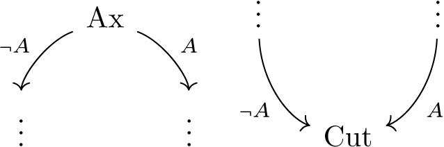
In both cases, we use the fact that
 $\mathbb{S}(\neg A) = \mathbb{S}(A)$
. We define
$\mathbb{S}(\neg A) = \mathbb{S}(A)$
. We define
 $\mathbb{X}(l)$
to be the diagonal
$\mathbb{X}(l)$
to be the diagonal
 $\Delta _{\mathbb{S}(A)}$
and define
$\Delta _{\mathbb{S}(A)}$
and define
 $\iota _l$
to be the canonical morphism
$\iota _l$
to be the canonical morphism
 \begin{equation} \iota _l: \mathbb{X}(l) = \Delta _{\mathbb{S}(A)} \longrightarrow \mathbb{S}(\neg A) \times \mathbb{S}(A). \end{equation}
Tensor- or Par-link .
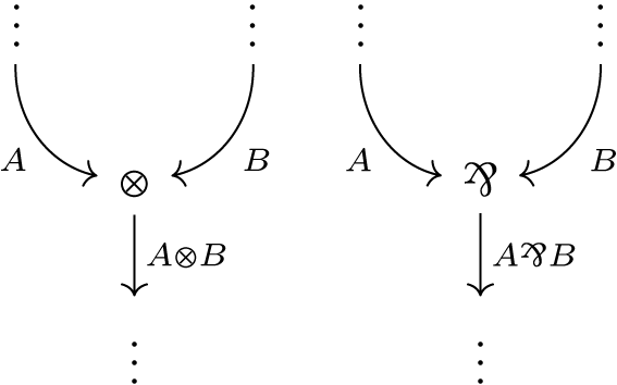
Let
 $\boxtimes \in \{\otimes , \unicode{x214B}\}$
. Write
$\boxtimes \in \{\otimes , \unicode{x214B}\}$
. Write
 $\mathbb{S}(A) = \coprod _{i \in I}\mathbb{P}^{r_i}, \mathbb{S}(B) = \coprod _{j \in J}\mathbb{P}^{s_j}$
. For each pair
$\mathbb{S}(A) = \coprod _{i \in I}\mathbb{P}^{r_i}, \mathbb{S}(B) = \coprod _{j \in J}\mathbb{P}^{s_j}$
. For each pair
 $(i,j) \in I \times J$
, there exists the Segre embedding
$(i,j) \in I \times J$
, there exists the Segre embedding
 \begin{equation} \mathbb{P}^{r_i} \times \mathbb{P}^{s_j} \longrightarrow \mathbb{P}^{(r_i + 1)(s_j + 1) - 1}. \end{equation}
We compose with the canonical inclusion morphism to obtain
 \begin{equation} \mathbb{P}^{r_i} \times \mathbb{P}^{s_j} \longrightarrow \coprod _{i \in I}\coprod _{j \in J}\mathbb{P}^{(r_i + 1)(s_j + 1) - 1} = \mathbb{S}(A \boxtimes B). \end{equation}
By the universal property of the coproduct, this induces a morphism
 \begin{equation} \coprod _{i \in I}\coprod _{j \in J}\mathbb{P}^{r_i} \times \mathbb{P}^{s_j} \longrightarrow \mathbb{S}(A \boxtimes B) \end{equation}
which we pre-compose with
 $\phi _{\operatorname {M}}^{-1}$
to obtain
$\phi _{\operatorname {M}}^{-1}$
to obtain
 \begin{equation} f: \mathbb{S}(A) \times \mathbb{S}(B) \longrightarrow \mathbb{S}(A \boxtimes B). \end{equation}
We take the graph
 $\Gamma _f$
of
$\Gamma _f$
of
 $f$
to be
$f$
to be
 $\mathbb{X}(l)$
and the canonical inclusion to be
$\mathbb{X}(l)$
and the canonical inclusion to be
 $\iota _l$
:
$\iota _l$
:
 \begin{equation} \iota _l: \mathbb{X}(l) = \Gamma _f \longrightarrow \mathbb{S}(A) \times \mathbb{S}(B) \times \mathbb{S}(A \boxtimes B). \end{equation}
Dereliction-link .
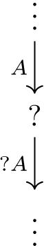
We have assumed that
 $\pi$
is shallow and so
$\pi$
is shallow and so
 $A$
is linear. Thus if
$A$
is linear. Thus if
 $m$
denotes the number of unoriented atoms of
$m$
denotes the number of unoriented atoms of
 $A$
, then
$A$
, then
 $\mathbb{S}(A) = \mathbb{P}^{2^m - 1}$
. Let
$\mathbb{S}(A) = \mathbb{P}^{2^m - 1}$
. Let
 $S$
denote the graded
$S$
denote the graded
 $\mathbb{k}$
-algebra
$\mathbb{k}$
-algebra
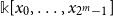 $\mathbb{k}[x_0, \ldots , x_{2^m - 1}]$
. For each
$\mathbb{k}[x_0, \ldots , x_{2^m - 1}]$
. For each
 $h \in \mathcal{H}$
, there exists an integer
$h \in \mathcal{H}$
, there exists an integer
 $s_h$
such that
$s_h$
such that
 $\mathbb{S}(?A) = \coprod _{h \in \mathcal{H}}\mathbb{P}^{s_h}$
. Fix
$\mathbb{S}(?A) = \coprod _{h \in \mathcal{H}}\mathbb{P}^{s_h}$
. Fix
 $h \in \mathcal{H}$
. Let
$h \in \mathcal{H}$
. Let
 $U = \operatorname {Spec}R$
denote an open affine of the Hilbert scheme
$U = \operatorname {Spec}R$
denote an open affine of the Hilbert scheme
 $H_{S}^h \subseteq \mathbb{P}^{r_s}$
, and consider the bijection
$H_{S}^h \subseteq \mathbb{P}^{r_s}$
, and consider the bijection
 \begin{equation} \psi : \underline {H_{S}^h}(R) \cong \operatorname {Hom}_{\underline {\operatorname {Sch}}_{\mathbb{k}}}(U, H_S^h) \end{equation}
coming from representability of the functor
 $\underline {H_{S}^h}$
(Theorem
2.3.15
).
$\underline {H_{S}^h}$
(Theorem
2.3.15
).
Associated to the inclusion
 $U \longrightarrow \underline {H_{S}^h}$
is an element
$U \longrightarrow \underline {H_{S}^h}$
is an element
 $I \in H_S^h(R)$
. This is a homogeneous ideal of
$I \in H_S^h(R)$
. This is a homogeneous ideal of
 $R \otimes S$
with Hilbert function
$R \otimes S$
with Hilbert function
 $h$
. This in turn corresponds to a closed immersion
$h$
. This in turn corresponds to a closed immersion
 \begin{equation} \mathbb{U}_{U }= \operatorname {Proj}((R \otimes S)/I) \longrightarrow \operatorname {Proj}(R \otimes S) \cong \operatorname {Spec}R \times \mathbb{S}(A). \end{equation}
By gluing along all open affines
 $U \subseteq H_{S}^h$
, we obtain a closed subscheme
$U \subseteq H_{S}^h$
, we obtain a closed subscheme
 \begin{equation} \iota : \mathbb{U}_h \longrightarrow H_S^h \times \mathbb{S}(A). \end{equation}
We post-compose with the product of the Grothendieck embedding
 $H_S^h \longrightarrow \mathbb{P}^{s_h}$
and the identity
$H_S^h \longrightarrow \mathbb{P}^{s_h}$
and the identity
 $\operatorname {id}: \mathbb{S}(A) \longrightarrow \mathbb{S}(A)$
:
$\operatorname {id}: \mathbb{S}(A) \longrightarrow \mathbb{S}(A)$
:
 \begin{equation} \mathbb{U}_h \longrightarrow \mathbb{P}^{s_h} \times \mathbb{S}(A). \end{equation}
We post-compose with the canonical inclusion:
 \begin{equation} \mathbb{U}_h \longrightarrow \coprod _{h \in \mathcal{H}}\big (\mathbb{P}^{s_h} \times \mathbb{S}(A)\big ). \end{equation}
We post-compose with
 $\phi ^{-1}_{\operatorname {D}}$
:
$\phi ^{-1}_{\operatorname {D}}$
:
 \begin{equation} \mathbb{U}_h \longrightarrow \mathbb{S}(?A) \times \mathbb{S}(A). \end{equation}
We take
 $\mathbb{X}(l)$
to be
$\mathbb{X}(l)$
to be
 $\coprod _{h \in \mathcal{H}}\mathbb{U}_h$
. By the universal property of the coproduct, this induces a morphism, which we take to be
$\coprod _{h \in \mathcal{H}}\mathbb{U}_h$
. By the universal property of the coproduct, this induces a morphism, which we take to be
 $\iota _l$
:
$\iota _l$
:
 \begin{equation} \iota _l: \mathbb{X}(l) = \coprod _{h \in \mathcal{H}}\mathbb{U}_h \longrightarrow \mathbb{S}(?A) \times \mathbb{S}(A). \end{equation}
Promotion-link .

Let
 $\zeta$
denote the proof net in the interior of the box. That is, let
$\zeta$
denote the proof net in the interior of the box. That is, let
 $\zeta$
be the proof net given by the interior of the box and replacing all Pax-links and the Promotion-link by Conclusion-links. Let
$\zeta$
be the proof net given by the interior of the box and replacing all Pax-links and the Promotion-link by Conclusion-links. Let
 $\mathcal{L}_\zeta$
denote the set of links of
$\mathcal{L}_\zeta$
denote the set of links of
 $\zeta$
. For each link
$\zeta$
. For each link
 $l \in \mathcal{L}_\zeta$
, the scheme
$l \in \mathcal{L}_\zeta$
, the scheme
 $\mathbb{X}(l)$
is a subscheme of some product of schemes associated to some edges of
$\mathbb{X}(l)$
is a subscheme of some product of schemes associated to some edges of
 $\zeta$
. Let
$\zeta$
. Let
 $E_l^c$
denote the edges of
$E_l^c$
denote the edges of
 $\zeta$
which are not in
$\zeta$
which are not in
 $\mathcal{L}_l$
, and let
$\mathcal{L}_l$
, and let
 $A_e$
denote the formula labelling an edge
$A_e$
denote the formula labelling an edge
 $e$
. Then there is a closed subscheme:
$e$
. Then there is a closed subscheme:
 \begin{equation} \prod _{e \in E_l^c}\mathbb{S}(A_e) \times \mathbb{X}(l) \longrightarrow \mathbb{S}(\zeta ). \end{equation}
We identify
 $\mathbb{X}(l)$
with this subscheme. The intersection of the subschemes associated to link
$\mathbb{X}(l)$
with this subscheme. The intersection of the subschemes associated to link
 $l \in \mathcal{L}_\zeta$
gives a subscheme
$l \in \mathcal{L}_\zeta$
gives a subscheme
 $\mathbb{X}(\zeta ) = \bigcap _{l \in \mathcal{L}_\zeta }\mathbb{X}(l) \longrightarrow \mathbb{S}(\zeta )$
.
$\mathbb{X}(\zeta ) = \bigcap _{l \in \mathcal{L}_\zeta }\mathbb{X}(l) \longrightarrow \mathbb{S}(\zeta )$
.
For each
 $i = 1, \ldots , n$
, let
$i = 1, \ldots , n$
, let
 $\{s_{h_i}\}_{h_i \in \mathcal{H}}$
denote the set of integers so that
$\{s_{h_i}\}_{h_i \in \mathcal{H}}$
denote the set of integers so that
 $\mathbb{S}(?A_i) = \coprod _{h_i \in \mathcal{H}} \mathbb{P}^{s_{h_i}}$
. We fix an element
$\mathbb{S}(?A_i) = \coprod _{h_i \in \mathcal{H}} \mathbb{P}^{s_{h_i}}$
. We fix an element
 $\textbf {h} = (h_1, \ldots , h_{n}) \in \mathcal{H}^n$
. For each
$\textbf {h} = (h_1, \ldots , h_{n}) \in \mathcal{H}^n$
. For each
 $i = 1, \ldots , n$
, we let
$i = 1, \ldots , n$
, we let
 $U_{i} = \operatorname {Spec}R_{i}$
be an open affine chart of
$U_{i} = \operatorname {Spec}R_{i}$
be an open affine chart of
 $H_{S_i}^{h_i}$
, where if
$H_{S_i}^{h_i}$
, where if
 $m_i$
denotes the number of unoriented atoms of (necessarily linear)
$m_i$
denotes the number of unoriented atoms of (necessarily linear)
 $A_i$
, then
$A_i$
, then
 $S_i = \mathbb{k}[x_0, \ldots , x_{2^{m_i}-1}]$
. Post-compose this with the inclusions
$S_i = \mathbb{k}[x_0, \ldots , x_{2^{m_i}-1}]$
. Post-compose this with the inclusions
 $H_{S_i}^{h_i} \longrightarrow \mathbb{P}^{h_{s_i}}$
, take the product with
$H_{S_i}^{h_i} \longrightarrow \mathbb{P}^{h_{s_i}}$
, take the product with
 $\operatorname {id}: \mathbb{S}(B) \longrightarrow \mathbb{S}(B)$
and take the product over all
$\operatorname {id}: \mathbb{S}(B) \longrightarrow \mathbb{S}(B)$
and take the product over all
 $i = 1, \ldots , n$
to obtain
$i = 1, \ldots , n$
to obtain
 \begin{equation} \prod _{i = 1}^n U_i \times \mathbb{S}(B) \longrightarrow \prod _{i = 1}^n\mathbb{P}^{h_{s_i}} \times \mathbb{S}(B). \end{equation}
We post-compose this with the canonical inclusion morphisms of the coproduct to obtain
 \begin{equation} \prod _{i = 1}^{n}U_{i} \times \mathbb{S}(B) \longrightarrow \coprod _{\textbf{h} \in \mathcal{H}^n} \Bigg (\prod _{i = 1}^{n} \mathbb{P}^{s_{h_i}} \times \mathbb{S}(B)\Bigg ) \end{equation}
which we post-compose with
 $\phi ^{-1}_{\operatorname {P}^1}$
to obtain
$\phi ^{-1}_{\operatorname {P}^1}$
to obtain
 \begin{equation} \prod _{i = 1}^n U_i \times \mathbb{S}(B) \longrightarrow \prod _{i = 1}^n \mathbb{S}(?A_i) \times \mathbb{S}(B). \end{equation}
We prove in Lemma 3.0.10 below that composing
 $\iota _\zeta : \mathbb{X}(\zeta ) \longrightarrow \mathbb{S}(\zeta )$
with the projection
$\iota _\zeta : \mathbb{X}(\zeta ) \longrightarrow \mathbb{S}(\zeta )$
with the projection
 $\rho _{\operatorname {Conc}}: \mathbb{S}(\zeta ) \longrightarrow \prod _{i = 1}^n \mathbb{S}(?A_i) \times \mathbb{S}(B)$
is a closed immersion
$\rho _{\operatorname {Conc}}: \mathbb{S}(\zeta ) \longrightarrow \prod _{i = 1}^n \mathbb{S}(?A_i) \times \mathbb{S}(B)$
is a closed immersion

We next consider the scheme
 $\mathbb{Y}_{\textbf {h}}$
such that the following is a pullback diagram:
$\mathbb{Y}_{\textbf {h}}$
such that the following is a pullback diagram:

Let
 $R = \bigotimes _{i = 1}^n R_i$
and fix a choice of isomorphism
$R = \bigotimes _{i = 1}^n R_i$
and fix a choice of isomorphism
 \begin{equation} \delta : \prod _{i = 1}^n U_i \longrightarrow \operatorname {Spec}R. \end{equation}
Let
 $m$
denote the number of unoriented atoms of
$m$
denote the number of unoriented atoms of
 $B$
and let
$B$
and let
 $S$
denote the graded
$S$
denote the graded
 $\mathbb{k}$
-module
$\mathbb{k}$
-module
 $\mathbb{k}[x_0, \ldots , x_{2^m - 1}]$
. Consider the closed immersion
$\mathbb{k}[x_0, \ldots , x_{2^m - 1}]$
. Consider the closed immersion

There exists a homogeneous saturated ideal
 $I \subseteq R \otimes S$
such that
$I \subseteq R \otimes S$
such that
 $\operatorname {Proj}((R \otimes S)/I) \cong \mathbb{Y}_{\textbf {h}}$
. It follows from the proof of Lemma 3.0.10 below that for all
$\operatorname {Proj}((R \otimes S)/I) \cong \mathbb{Y}_{\textbf {h}}$
. It follows from the proof of Lemma 3.0.10 below that for all
 $d \geq 0$
, the
$d \geq 0$
, the
 $R$
-module
$R$
-module
 $(R \otimes S/I)_d$
is locally free of rank
$(R \otimes S/I)_d$
is locally free of rank
 $h(d)$
, where
$h(d)$
, where
 $h$
is the Hilbert function of
$h$
is the Hilbert function of
 $I \subseteq R \otimes S$
. Thus
$I \subseteq R \otimes S$
. Thus
 $I \in \underline {H_{S}^h}(R)$
. Since the Hilbert functor is represented by the scheme
$I \in \underline {H_{S}^h}(R)$
. Since the Hilbert functor is represented by the scheme
 $H_S^h$
, the ideal
$H_S^h$
, the ideal
 $I$
corresponds to a morphism
$I$
corresponds to a morphism
 \begin{equation} \operatorname {Spec}R \longrightarrow H_S^h. \end{equation}
We pre-compose this with
 $\delta$
to obtain
$\delta$
to obtain
 \begin{equation} \prod _{i =1}^{n} U_i \longrightarrow H_{S}^h. \end{equation}
This is a morphism depending on choices of open affines
 $U_{1}, \ldots , U_{n}$
of
$U_{1}, \ldots , U_{n}$
of
 $H_{S_1}^{h_1}, \ldots , H_{S_n}^{h_n}$
, respectively. By ranging over all such choices, we obtain a family of morphisms which we can glue to obtain the following:
$H_{S_1}^{h_1}, \ldots , H_{S_n}^{h_n}$
, respectively. By ranging over all such choices, we obtain a family of morphisms which we can glue to obtain the following:
 \begin{equation} f_{\textbf {h}}: \prod _{i = 1}^{n}H_{S_i}^{h_i} \longrightarrow H_{S}^h. \end{equation}
We consider the graph of this:
 \begin{equation} \Gamma _{f_{\textbf {h}}} \longrightarrow \prod _{i = 1}^n H_{S_i}^{h_i} \times H_S^h. \end{equation}
For each
 $i = 1, \ldots , n$
, there is the Grothendieck immersion
$i = 1, \ldots , n$
, there is the Grothendieck immersion
 $H_{S_i}^{h_i}\longrightarrow \mathbb{P}^{s_{h_i}}$
. Similarly, for each
$H_{S_i}^{h_i}\longrightarrow \mathbb{P}^{s_{h_i}}$
. Similarly, for each
 $h \in \mathcal{H}$
, there is the Grothendieck immersion
$h \in \mathcal{H}$
, there is the Grothendieck immersion
 $H_S^h \longrightarrow \mathbb{P}^{s_h}$
for some
$H_S^h \longrightarrow \mathbb{P}^{s_h}$
for some
 $s_h$
. We post-compose with the product of these to obtain
$s_h$
. We post-compose with the product of these to obtain
 \begin{equation} \Gamma _{f_{\textbf {h}}} \longrightarrow \prod _{i = 1}^n \mathbb{P}^{s_{h_i}} \times \mathbb{P}^{s_h}. \end{equation}
We then post-compose with the canonical inclusion morphisms to obtain
 \begin{equation} \Gamma _{f_{\textbf {h}}} \longrightarrow \coprod _{\boldsymbol{h} \in \mathcal{H}^n}\coprod _{h \in \mathcal{H}} \Bigg (\prod _{i = 1}^n \mathbb{P}^{h_i} \times \mathbb{P}^{s_h}\Bigg ). \end{equation}
Ranging over all
 $\textbf {h}$
, we get a disjoint union, which we denote
$\textbf {h}$
, we get a disjoint union, which we denote
 $\Gamma _f$
 \begin{equation} \Gamma _f = \coprod _{\textbf {h} \in H^n}\Gamma _{f_{\textbf {h}}} \longrightarrow \coprod _{\boldsymbol{h} \in \mathcal{H}^n}\coprod _{h \in \mathcal{H}} \Bigg (\prod _{i = 1}^n \mathbb{P}^{h_i} \times \mathbb{P}^{s_h}\Bigg ). \end{equation}
We post-compose with
 $\phi _{\operatorname {P}^2}^{-1}$
. We take
$\phi _{\operatorname {P}^2}^{-1}$
. We take
 $\mathbb{X}(l)$
to be
$\mathbb{X}(l)$
to be
 $\Gamma _f$
and take
$\Gamma _f$
and take
 $\iota _l$
to be:
$\iota _l$
to be:
 \begin{equation} \iota _l: \mathbb{X}(l) = \Gamma _f \longrightarrow \prod _{i = 1}^n\mathbb{S}(?A_i) \times \mathbb{S}(!B). \end{equation}
Weakening-link.
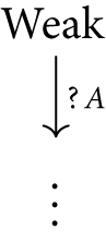
We take the empty subscheme
 $\varnothing$
for
$\varnothing$
for
 $\mathbb{X}(l)$
and the unique morphism
$\mathbb{X}(l)$
and the unique morphism
 $\varnothing \longrightarrow \mathbb{S}(!A)$
for
$\varnothing \longrightarrow \mathbb{S}(!A)$
for
 $\iota _l$
:
$\iota _l$
:
 \begin{equation} \iota _l: \mathbb{X}(l) = \varnothing \longrightarrow \mathbb{S}(?A). \end{equation}
Contraction-link.
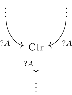
Let
 $\Gamma _{\Delta }$
be the graph of the diagonal
$\Gamma _{\Delta }$
be the graph of the diagonal
 $\Delta : \mathbb{S}(?A) \longrightarrow \mathbb{S}(?A) \times \mathbb{S}(?A)$
. We take this to be
$\Delta : \mathbb{S}(?A) \longrightarrow \mathbb{S}(?A) \times \mathbb{S}(?A)$
. We take this to be
 $\mathbb{X}(l)$
, and
$\mathbb{X}(l)$
, and
 $\iota _l$
to be the canonical inclusion:
$\iota _l$
to be the canonical inclusion:
 \begin{equation} \iota _l: \mathbb{X}(l) = \Gamma _\Delta \longrightarrow \mathbb{S}(?A) \times \mathbb{S}(?A) \times \mathbb{S}(?A). \end{equation}
Pax-link .
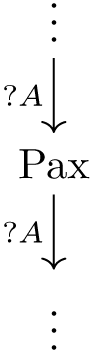
We define
 $\mathbb{X}(l)$
to be the diagonal
$\mathbb{X}(l)$
to be the diagonal
 $\Delta _{\mathbb{S}(?A)}$
and define
$\Delta _{\mathbb{S}(?A)}$
and define
 $\iota _l$
to be the canonical morphism:
$\iota _l$
to be the canonical morphism:
 \begin{equation} \iota _l: \mathbb{X}(l) = \Delta _{\mathbb{S}(?A)} \longrightarrow \mathbb{S}(?A) \times \mathbb{S}(?A). \end{equation}
Definition 3.0.6.
Let
 $\pi$
be a proof net with set of links
$\pi$
be a proof net with set of links
 $\mathcal{L}_\pi$
. For each link
$\mathcal{L}_\pi$
. For each link
 $l \in \mathcal{L}_\pi$
, the scheme
$l \in \mathcal{L}_\pi$
, the scheme
 $\mathbb{X}(l)$
is a subscheme of some product of schemes associated to some edges of
$\mathbb{X}(l)$
is a subscheme of some product of schemes associated to some edges of
 $\pi$
associated with
$\pi$
associated with
 $l$
. Let
$l$
. Let
 $E_l^c$
denote the edges of
$E_l^c$
denote the edges of
 $\pi$
, which are not incident to
$\pi$
, which are not incident to
 $l$
, and let
$l$
, and let
 $A_e$
denote the formula labelling an edge
$A_e$
denote the formula labelling an edge
 $e$
. Then there is a closed subscheme
$e$
. Then there is a closed subscheme
 \begin{equation} \prod _{e \in E_l^c}\mathbb{S}(A_e) \times \mathbb{X}(l) \longrightarrow \mathbb{S}(\pi ). \end{equation}
We identify
 $\mathbb{X}(l)$
with this subscheme. The
scheme associated to
$\mathbb{X}(l)$
with this subscheme. The
scheme associated to
 $\pi$
is the intersection of all schemes associated to the links:
$\pi$
is the intersection of all schemes associated to the links:
 \begin{equation} \mathbb{X}(\pi ) = \bigcap _{l \in \mathcal{L}_\pi }\mathbb{X}(l). \end{equation}
To prove the prerequisite lemmas used in Definition 3.0.5, we will make use of the Cartesian product, which is the algebraic equivalent to the product in the category of projective schemes.
Definition 3.0.7.
Let
 $S,T$
be graded
$S,T$
be graded
 $\mathbb{k}$
-algebras. We define their
Cartesian product
, denoted
$\mathbb{k}$
-algebras. We define their
Cartesian product
, denoted
 $S \times _{\mathbb{k}} T$
, to be the following graded
$S \times _{\mathbb{k}} T$
, to be the following graded
 $\mathbb{k}$
-algebra: as a
$\mathbb{k}$
-algebra: as a
 $\mathbb{k}$
-module it is the sum of the images of the
$\mathbb{k}$
-module it is the sum of the images of the
 $\mathbb{k}$
-module morphisms
$\mathbb{k}$
-module morphisms
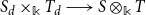 $S_d \times _{\mathbb{k}} T_d \longrightarrow S \otimes _{\mathbb{k}}T$
for all
$S_d \times _{\mathbb{k}} T_d \longrightarrow S \otimes _{\mathbb{k}}T$
for all
 $d \geq 0$
. This is a
$d \geq 0$
. This is a
 $\mathbb{k}$
-subalgebra of
$\mathbb{k}$
-subalgebra of
 $S \otimes _{\mathbb{k}} T$
, which is a graded
$S \otimes _{\mathbb{k}} T$
, which is a graded
 $\mathbb{k}$
-algebra with grading
$\mathbb{k}$
-algebra with grading
 $(S \times _{\mathbb{k}} T)_d \cong S_d \otimes _{\mathbb{k}} T_d$
for
$(S \times _{\mathbb{k}} T)_d \cong S_d \otimes _{\mathbb{k}} T_d$
for
 $d \geq 0$
.
$d \geq 0$
.
Proposition 3.0.8.
Let
 $S,T$
be graded
$S,T$
be graded
 $\mathbb{k}$
-algebras, and suppose that
$\mathbb{k}$
-algebras, and suppose that
 $S$
is generated by
$S$
is generated by
 $S_1$
as an
$S_1$
as an
 $S_0$
-algebra and that
$S_0$
-algebra and that
 $T$
is generated by
$T$
is generated by
 $T_1$
as a
$T_1$
as a
 $T_0$
-algebra. Then
$T_0$
-algebra. Then
 $\operatorname {Proj}(S \times _{\mathbb{k}} T) \cong \operatorname {Proj}S \times \operatorname {Proj}T$
.
$\operatorname {Proj}(S \times _{\mathbb{k}} T) \cong \operatorname {Proj}S \times \operatorname {Proj}T$
.
Proof. See Hartshorne (Reference Hartshorne1977, Exercise 5.11).
Lemma 3.0.9.
Let
 $\zeta$
be an MLL proof net with conclusions
$\zeta$
be an MLL proof net with conclusions
 $A_1, \ldots , A_n$
. If
$A_1, \ldots , A_n$
. If
 $\rho _{\text{Conc}}: \mathbb{S}(\zeta ) \longrightarrow \prod _{i = 1}^n \mathbb{S}(A_i)$
denotes the standard projection, then the composite
$\rho _{\text{Conc}}: \mathbb{S}(\zeta ) \longrightarrow \prod _{i = 1}^n \mathbb{S}(A_i)$
denotes the standard projection, then the composite

is a closed immersion.
Moreover, if
 $m_i$
is the number of unoriented atoms of
$m_i$
is the number of unoriented atoms of
 $A_i$
,
$A_i$
,
 $S$
denotes the graded
$S$
denotes the graded
 $\mathbb{k}$
-algebra
$\mathbb{k}$
-algebra
 \begin{equation} S = \mathbb{k}[x_0,\ldots , x_{2^{m_1}-1}] \times _{\mathbb{k}} \ldots \times _{\mathbb{k}} \mathbb{k}[x_0,\ldots , x_{2^{m_n}-1}] \end{equation}
and
 $I \subseteq S$
is the unique saturated homogeneous ideal such that
$I \subseteq S$
is the unique saturated homogeneous ideal such that
 \begin{equation} \operatorname {Proj}(S/I) \cong \mathbb{X}(\zeta ) \end{equation}
then for all
 $d \geq 0$
,
$d \geq 0$
,
 $(S/I)_d$
is locally free.
$(S/I)_d$
is locally free.
Proof.
We prove the
 $n = 1$
case where
$n = 1$
case where
 $\zeta$
has a unique conclusion
$\zeta$
has a unique conclusion
 $A = A_1$
.
$A = A_1$
.
Since
 $\zeta$
is a proof net,
$\zeta$
is a proof net,
 $m = 2m'$
is even. The proof net
$m = 2m'$
is even. The proof net
 $\zeta$
admits
$\zeta$
admits
 $m'$
persistent paths which begin with a positively oriented formula. We prove the
$m'$
persistent paths which begin with a positively oriented formula. We prove the
 $m' = 1$
case.
$m' = 1$
case.
Let
 $Z_1, \ldots , Z_s$
denote the persistent path which begins with a positively oriented formula. For each formula
$Z_1, \ldots , Z_s$
denote the persistent path which begins with a positively oriented formula. For each formula
 $B_j$
in
$B_j$
in
 $\pi$
, there is an integer
$\pi$
, there is an integer
 $t_j \geq 1$
and a sequence of atoms
$t_j \geq 1$
and a sequence of atoms
 $\textbf {X}_j = X_j^1, \ldots , X_j^{t_j}$
such that the concatenation
$\textbf {X}_j = X_j^1, \ldots , X_j^{t_j}$
such that the concatenation
 $\textbf {X}_1, \ldots , \textbf {X}_l$
of these sequences is the persistent path
$\textbf {X}_1, \ldots , \textbf {X}_l$
of these sequences is the persistent path
 $Z_1, \ldots , Z_s$
, with
$Z_1, \ldots , Z_s$
, with
 $s = \sum _{j = 1}^l t_j$
.
$s = \sum _{j = 1}^l t_j$
.
We have commutativity of the following diagram, where the diagonal arrow is a closed immersion:
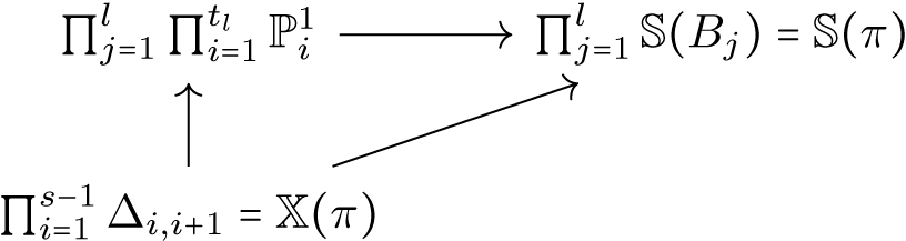
where
 $\mathbb{P}^1_i$
denotes the copy of
$\mathbb{P}^1_i$
denotes the copy of
 $\mathbb{P}^1$
pertaining to
$\mathbb{P}^1$
pertaining to
 $Z_i$
.
$Z_i$
.
Now consider the following commutative diagram, where the left and middle vertical arrows are induced by the right-most vertical arrow
 $\rho _{\text{conc}}$
:
$\rho _{\text{conc}}$
:

The first claim follows from the observation that the left-most vertical morphism in (84) is an isomorphism, and the bottom horizontal morphisms are closed immersions.
We have computed
 $\mathbb{X}(\zeta )$
as
$\mathbb{X}(\zeta )$
as
 $\Delta _{1,s} \longrightarrow \mathbb{P}^3$
, so we can write down generators for
$\Delta _{1,s} \longrightarrow \mathbb{P}^3$
, so we can write down generators for
 $I$
explicitly:
$I$
explicitly:
 \begin{equation} I = (Z_{00}Z_{11} - Z_{01}Z_{10}, Z_{01} - Z_{10})\subseteq \mathbb{k}[Z_{00}, Z_{01}, Z_{10}, Z_{11}]. \end{equation}
For each
 $d \geq 0$
, the module
$d \geq 0$
, the module
 $(\mathbb{k}[Z_{00}, Z_{01}, Z_{10}, Z_{11}]/I)_d$
is a free
$(\mathbb{k}[Z_{00}, Z_{01}, Z_{10}, Z_{11}]/I)_d$
is a free
 $\mathbb{k}$
-module.
$\mathbb{k}$
-module.
The following lemma is used in Definition 3.0.4, in the Promotion-link clause. There, we used the fact that the interior of a box inside a shallow proof net corresponds to an ideal of the right from to induce a morphism into the projective scheme representing the Hilbert scheme. Since we only consider shallow proofs, we do not allow for Weakening-links to appear inside boxes (as nested boxes are forbidden), so we may assume in the following lemma that
 $\zeta$
admits no Weakening-links.
$\zeta$
admits no Weakening-links.
Lemma 3.0.10.
Let
 $\zeta$
be a nearly linear proof with conclusions
$\zeta$
be a nearly linear proof with conclusions
 $?A_1, \ldots , ?A_n, B$
. For each
$?A_1, \ldots , ?A_n, B$
. For each
 $i = 1, \ldots , n$
, let
$i = 1, \ldots , n$
, let
 $\{s_{h_i}\}_{h_i \in \mathcal{H}}$
denote the set of integers so that
$\{s_{h_i}\}_{h_i \in \mathcal{H}}$
denote the set of integers so that
 $\mathbb{S}(?A_i) = \coprod _{h_i \in \mathcal{H}} \mathbb{P}^{s_{h_i}}$
. Let
$\mathbb{S}(?A_i) = \coprod _{h_i \in \mathcal{H}} \mathbb{P}^{s_{h_i}}$
. Let
 $\textbf{h} = (h_1, \ldots , h_n)$
be an element of
$\textbf{h} = (h_1, \ldots , h_n)$
be an element of
 $\mathcal{H}^n$
. Let
$\mathcal{H}^n$
. Let
 $\rho _{\textbf {Conc}}: \mathbb{S}(\zeta ) \longrightarrow \prod _{i = 1}^n \mathbb{S}(?A_i) \times \mathbb{S}(B)$
denote the standard projection. Consider the following pullback diagram:
$\rho _{\textbf {Conc}}: \mathbb{S}(\zeta ) \longrightarrow \prod _{i = 1}^n \mathbb{S}(?A_i) \times \mathbb{S}(B)$
denote the standard projection. Consider the following pullback diagram:
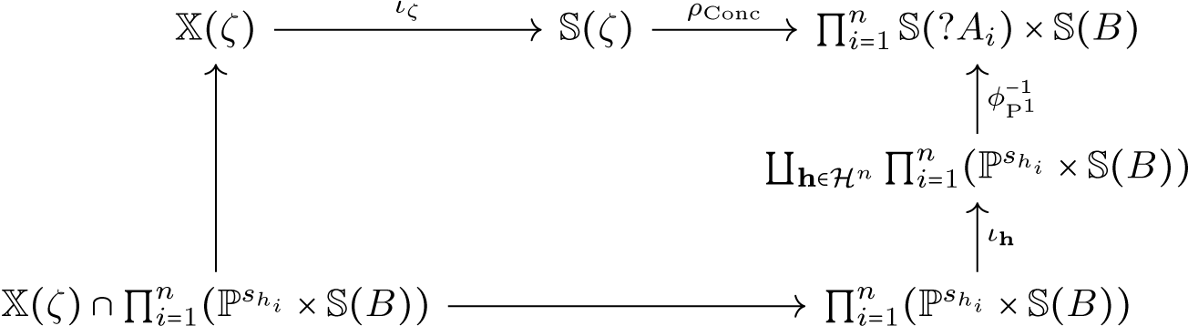
where
 $\iota _{\textbf {h}}$
is the standard inclusion and
$\iota _{\textbf {h}}$
is the standard inclusion and
 $\phi ^{-1}_{\operatorname {P}^1}$
is the isomorphism of (
43
). Then the composite
$\phi ^{-1}_{\operatorname {P}^1}$
is the isomorphism of (
43
). Then the composite

is a closed immersion. Moreover, if
 $m$
denotes the number of unoriented atoms in
$m$
denotes the number of unoriented atoms in
 $B$
and
$B$
and
 $S$
denotes the graded
$S$
denotes the graded
 $\mathbb{k}$
-algebra
$\mathbb{k}$
-algebra
 \begin{equation} S = \mathbb{k}[x_0, \ldots , x_{s_{h_1}}] \times _{\mathbb{k}} \ldots \times _{\mathbb{k}} \mathbb{k}[x_0, \ldots , x_{s_{h_n}}] \times _{\mathbb{k}} \mathbb{k}[x_0, \ldots , x_{m}] \end{equation}
and
 $I$
the unique saturated homogeneous ideal such that
$I$
the unique saturated homogeneous ideal such that
 \begin{equation} \operatorname {Proj}(S/I) \cong \mathbb{X}(\zeta ) \end{equation}
then for all
 $d \geq 0$
,
$d \geq 0$
,
 $(S/I)_d$
is locally free.
$(S/I)_d$
is locally free.
Proof.
Contraction-links trivially introduce isomorphisms, which may be ignored, and so we assume that
 $\zeta$
is Contraction-free. Thus,
$\zeta$
is Contraction-free. Thus,
 $\zeta$
is of the following form:
$\zeta$
is of the following form:
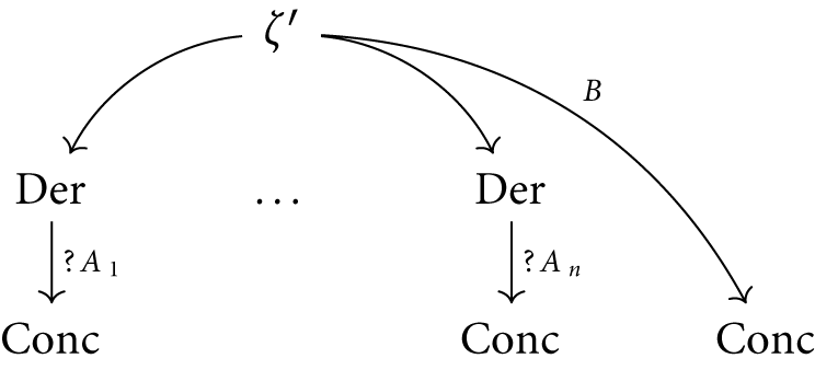
where
 $\zeta '$
is the linear part (Definition 2.0.3) of the nearly linear proof
$\zeta '$
is the linear part (Definition 2.0.3) of the nearly linear proof
 $\zeta$
.
$\zeta$
.
By Lemma 3.0.9, we have that the canonical projection
 \begin{equation} \mathbb{X}(\zeta ') \longrightarrow \prod _{i = 1}^n\mathbb{S}(A_i) \times \mathbb{S}(B) \end{equation}
is a closed immersion. For each
 $i = 1, \ldots , n$
, let
$i = 1, \ldots , n$
, let
 $\mathbb{U}_{h_i} \longrightarrow \mathbb{P}^{s_{h_i}} \times \mathbb{S}(A_i)$
be the closed immersion of the universal closed subscheme as given in (56). Then
$\mathbb{U}_{h_i} \longrightarrow \mathbb{P}^{s_{h_i}} \times \mathbb{S}(A_i)$
be the closed immersion of the universal closed subscheme as given in (56). Then
is a closed immersion (being the pullback of two closed immersions).
Each
 $A_i$
as well as
$A_i$
as well as
 $B$
is linear. Let
$B$
is linear. Let
 $m_1, \ldots , m_n,m$
, respectively, denote the number of unoriented atoms of
$m_1, \ldots , m_n,m$
, respectively, denote the number of unoriented atoms of
 $A_1, \ldots , A_n, B$
. Let
$A_1, \ldots , A_n, B$
. Let
 $f: \mathbb{N} \longrightarrow \mathbb{N}$
denote the function given by the equation
$f: \mathbb{N} \longrightarrow \mathbb{N}$
denote the function given by the equation
 $f(n) \longmapsto$
 $2^n-1$
, then
$2^n-1$
, then
 \begin{equation} \mathbb{S}(A_i) = \mathbb{P}^{f(m_i)},\quad \mathbb{S}(B) = \mathbb{P}^{f(m)}. \end{equation}
The integer
 $\sum _{i=1}^nm_i + m$
is the number of unoriented atoms in the conclusions of a MLL proof net, and thus is necessarily even. Let
$\sum _{i=1}^nm_i + m$
is the number of unoriented atoms in the conclusions of a MLL proof net, and thus is necessarily even. Let
 $p$
denote half this number. We saw in the proof of Lemma 3.0.9 that there is a factorisation:
$p$
denote half this number. We saw in the proof of Lemma 3.0.9 that there is a factorisation:
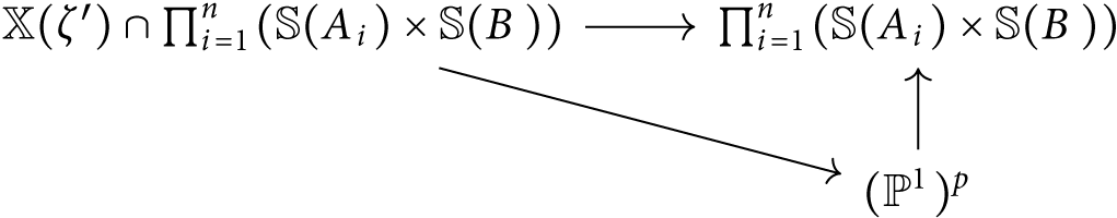
This implies that there exists the following factorisation:
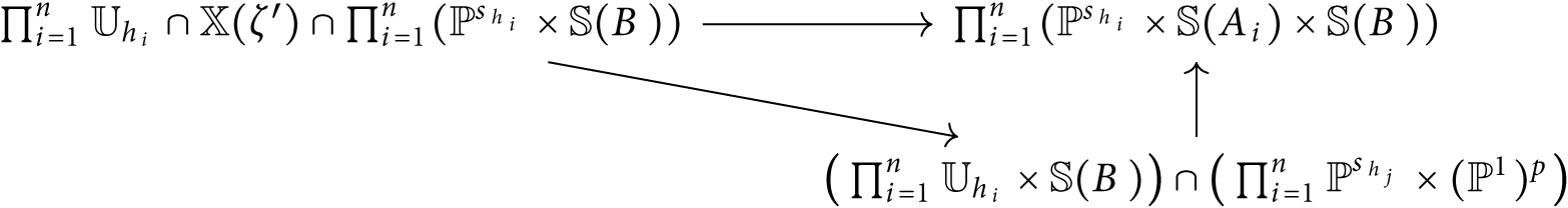
We have assumed that
 $\zeta$
is shallow, and so all persistent paths of
$\zeta$
is shallow, and so all persistent paths of
 $\zeta '$
go through
$\zeta '$
go through
 $B$
. This implies that
$B$
. This implies that
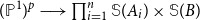 $(\mathbb{P}^1)^p \longrightarrow \prod _{i = 1}^n\mathbb{S}(A_i) \times \mathbb{S}(B)$
can be realised as a closed subscheme of
$(\mathbb{P}^1)^p \longrightarrow \prod _{i = 1}^n\mathbb{S}(A_i) \times \mathbb{S}(B)$
can be realised as a closed subscheme of
 $\mathbb{S}(B)$
. We thus have the following factorisation:
$\mathbb{S}(B)$
. We thus have the following factorisation:
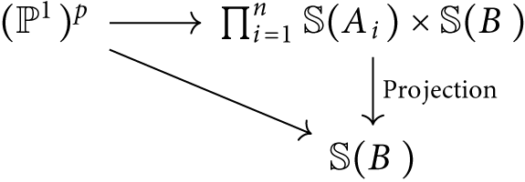
where the diagonal arrow is a closed immersion. This implies the existence of the following factorisation:
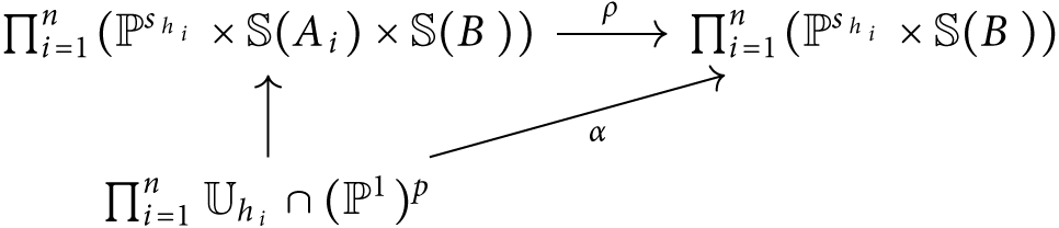
where
 $\rho$
is a product of projections and
$\rho$
is a product of projections and
 $\alpha$
is a closed immersion.
$\alpha$
is a closed immersion.
The final claim follows from the fact that
 $\prod _{i = 1}^n \mathbb{U}_{h_i} \cap (\mathbb{P}^1)^p \longrightarrow \prod _{i = 1}^n\mathbb{S}(?A_i) \times \mathbb{S}(B)$
is an intersection of closed subschemes of the right form.
$\prod _{i = 1}^n \mathbb{U}_{h_i} \cap (\mathbb{P}^1)^p \longrightarrow \prod _{i = 1}^n\mathbb{S}(?A_i) \times \mathbb{S}(B)$
is an intersection of closed subschemes of the right form.
Remark 3.0.11. We remark that Lemma 3.0.10 is the main hurdle in extending our model beyond shallow proofs and to all MELL proofs. We commented on this already in Remark 2.3.29 and we will again in Section 4.
3.1 Invariance under cut-elimination
Now that we have defined the locally closed subscheme
 $\mathbb{X}(\pi )$
of
$\mathbb{X}(\pi )$
of
 $\mathbb{S}(\pi )$
to each shallow proof net
$\mathbb{S}(\pi )$
to each shallow proof net
 $\pi$
, we now move onto considering how the schemes
$\pi$
, we now move onto considering how the schemes
 $\mathbb{X}(\pi )$
and
$\mathbb{X}(\pi )$
and
 $\mathbb{X}(\pi ')$
are related if
$\mathbb{X}(\pi ')$
are related if
 $\pi '$
is a shallow proof net obtained from
$\pi '$
is a shallow proof net obtained from
 $\pi$
via single step cut-reduction. The main result of this paper is Theorem3.1.3, which extends (Murfet and Troiani Reference Murfet and Troiani2022, Proposition 4.6).
$\pi$
via single step cut-reduction. The main result of this paper is Theorem3.1.3, which extends (Murfet and Troiani Reference Murfet and Troiani2022, Proposition 4.6).
Definition 3.1.1.
For each reduction
 $\gamma : \pi \longrightarrow \pi '$
, we define a closed subscheme
$\gamma : \pi \longrightarrow \pi '$
, we define a closed subscheme
 $\mathbb{Y}(\pi ') \subseteq \mathbb{S}(\pi ')$
and a pair of morphisms of schemes
$\mathbb{Y}(\pi ') \subseteq \mathbb{S}(\pi ')$
and a pair of morphisms of schemes
 $S_\gamma : \mathbb{S}(\pi ) \longrightarrow \mathbb{S}(\pi ')$
,
$S_\gamma : \mathbb{S}(\pi ) \longrightarrow \mathbb{S}(\pi ')$
,
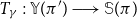 $T_\gamma : \mathbb{Y}(\pi ') \longrightarrow \mathbb{S}(\pi )$
.
$T_\gamma : \mathbb{Y}(\pi ') \longrightarrow \mathbb{S}(\pi )$
.
Let
 $\gamma : \pi \longrightarrow \pi '$
be a reduction. Let
$\gamma : \pi \longrightarrow \pi '$
be a reduction. Let
 $\mathcal{E}_\pi$
denote the set of edges of
$\mathcal{E}_\pi$
denote the set of edges of
 $\pi$
, and
$\pi$
, and
 $\mathcal{E}_{\pi '}$
that of
$\mathcal{E}_{\pi '}$
that of
 $\pi '$
.
$\pi '$
.
 $\gamma : \pi \longrightarrow \pi '$
is an
$\gamma : \pi \longrightarrow \pi '$
is an
 $\operatorname {Ax}/\operatorname {Cut}$
-reduction.
We set
$\operatorname {Ax}/\operatorname {Cut}$
-reduction.
We set
 $\mathbb{Y}(\pi ') = \mathbb{S}(\pi ')$
. Consider the following reduction where the labels
$\mathbb{Y}(\pi ') = \mathbb{S}(\pi ')$
. Consider the following reduction where the labels
 $a,b,c,d$
are artificial:
$a,b,c,d$
are artificial:

For the edge
 $e$
of
$e$
of
 $\pi '$
labelled
$\pi '$
labelled
 $\neg A_d$
in (
90
), let
$\neg A_d$
in (
90
), let
 $\rho _e$
denote the projection
$\rho _e$
denote the projection
 $\rho _e: \mathbb{S}(\pi ) \longrightarrow \mathbb{S}(\neg A_c)$
. For every edge
$\rho _e: \mathbb{S}(\pi ) \longrightarrow \mathbb{S}(\neg A_c)$
. For every edge
 $e$
of
$e$
of
 $\pi '$
which is not displayed in (
90
), there is a corresponding edge
$\pi '$
which is not displayed in (
90
), there is a corresponding edge
 $e'$
of
$e'$
of
 $\pi$
. For these, set
$\pi$
. For these, set
 $\rho _e$
to be the projection
$\rho _e$
to be the projection
 $\rho _e: \mathbb{S}(\pi ) \longrightarrow \mathbb{S}(A_{e'})$
. We define
$\rho _e: \mathbb{S}(\pi ) \longrightarrow \mathbb{S}(A_{e'})$
. We define
 $S_{\gamma }: \mathbb{S}(\pi ) \longrightarrow \mathbb{S}(\pi ')$
to be the morphism induced by the universal property of the product and the set
$S_{\gamma }: \mathbb{S}(\pi ) \longrightarrow \mathbb{S}(\pi ')$
to be the morphism induced by the universal property of the product and the set
 $\{\rho _e\}_{e \in \mathcal{E}_{\pi '}}$
.
$\{\rho _e\}_{e \in \mathcal{E}_{\pi '}}$
.
For the edges
 $e$
of
$e$
of
 $\pi$
displayed in (
90
) labelled
$\pi$
displayed in (
90
) labelled
 $\neg A_a, A_b, \neg A_c$
, let
$\neg A_a, A_b, \neg A_c$
, let
 $\tau _e$
denote the projection
$\tau _e$
denote the projection
 $\mathbb{S}(\pi ') \longrightarrow \mathbb{S}(\neg A_d)$
. For every edge
$\mathbb{S}(\pi ') \longrightarrow \mathbb{S}(\neg A_d)$
. For every edge
 $e$
of
$e$
of
 $\pi$
which is not displayed in (
91
), there is a corresponding edge
$\pi$
which is not displayed in (
91
), there is a corresponding edge
 $e'$
of
$e'$
of
 $\pi '$
. For these set
$\pi '$
. For these set
 $\tau _e$
to be the projection
$\tau _e$
to be the projection
 $\tau _e: \mathbb{S}(\pi ') \longrightarrow \mathbb{S}(A_{e'})$
. We define
$\tau _e: \mathbb{S}(\pi ') \longrightarrow \mathbb{S}(A_{e'})$
. We define
 $T_{\gamma }: \mathbb{S}(\pi ') \longrightarrow \mathbb{S}(\pi )$
to be the morphism induced by the universal property of the product and the set
$T_{\gamma }: \mathbb{S}(\pi ') \longrightarrow \mathbb{S}(\pi )$
to be the morphism induced by the universal property of the product and the set
 $\{\tau _e\}_{e \in \mathcal{E}_{\pi }}$
.
$\{\tau _e\}_{e \in \mathcal{E}_{\pi }}$
.
 $\gamma : \pi \longrightarrow \pi '$
is a
$\gamma : \pi \longrightarrow \pi '$
is a
 $\otimes /\unicode{x214B}$
-reduction.
We set
$\otimes /\unicode{x214B}$
-reduction.
We set
 $\mathbb{Y}(\pi ') = \mathbb{S}(\pi ')$
. Consider the following reduction where the labels are artificial:
$\mathbb{Y}(\pi ') = \mathbb{S}(\pi ')$
. Consider the following reduction where the labels are artificial:

For the edges of
 $\pi '$
displayed in (
91
), define a morphism
$\pi '$
displayed in (
91
), define a morphism
 $\rho _e$
to be a projection according to the following table:
$\rho _e$
to be a projection according to the following table:
| Edge label |
 $\rho _e$
|
|---|---|
 $B_h$
$B_h$
|
 $\mathbb{S}(\pi ) \longrightarrow \mathbb{S}(B_b)$
|
 $\neg B_i$
|
 $\mathbb{S}(\pi ) \longrightarrow \mathbb{S}(\neg B_c)$
|
 $A_j$
$A_j$
|
 $\mathbb{S}(\pi ) \longrightarrow \mathbb{S}(A_a)$
|
 $\neg A_k$
|
 $\mathbb{S}(\pi ) \longrightarrow \mathbb{S}(\neg A_d)$
|

For every edge
 $e$
of
$e$
of
 $\pi '$
which is not displayed in (
91
), there is a corresponding edge
$\pi '$
which is not displayed in (
91
), there is a corresponding edge
 $e'$
of
$e'$
of
 $\pi$
. For these, set
$\pi$
. For these, set
 $\rho _e$
to be the projection
$\rho _e$
to be the projection
 $\mathbb{S}(\pi ) \longrightarrow \mathbb{S}(A_{e'})$
. We define
$\mathbb{S}(\pi ) \longrightarrow \mathbb{S}(A_{e'})$
. We define
 $S_{\gamma }: \mathbb{S}(\pi ) \longrightarrow \mathbb{S}(\pi ')$
to be the morphism induced by the universal property of the product and the set
$S_{\gamma }: \mathbb{S}(\pi ) \longrightarrow \mathbb{S}(\pi ')$
to be the morphism induced by the universal property of the product and the set
 $\{\rho _e\}_{e \in \mathcal{E}_{\pi '}}$
.
$\{\rho _e\}_{e \in \mathcal{E}_{\pi '}}$
.
For the following edges of
 $\pi$
displayed in (
91
), define a morphism
$\pi$
displayed in (
91
), define a morphism
 $\tau _e$
to be a projection according to the following table:
$\tau _e$
to be a projection according to the following table:
| Edge label |
 $\tau _e$
|
|---|---|
 $A_a$
$A_a$
|
 $\mathbb{S}(\pi ') \longrightarrow \mathbb{S}(A_j)$
|
 $B_b$
$B_b$
|
 $\mathbb{S}(\pi ') \longrightarrow \mathbb{S}(B_h)$
|
 $\neg B_c$
|
 $\mathbb{S}(\pi ') \longrightarrow \mathbb{S}(\neg B_i)$
|
 $\neg A_d$
|
 $\mathbb{S}(\pi ') \longrightarrow \mathbb{S}(\neg A_k)$
|

For the edge
 $e$
labelled
$e$
labelled
 $(A \otimes B)_f$
, say
$(A \otimes B)_f$
, say
 $\mathbb{S}(A) = \coprod _{i \in I}\mathbb{P}^{r_i}, \mathbb{S}(B) = \coprod _{j \in J}\mathbb{P}^{s_j}$
. For each pair
$\mathbb{S}(A) = \coprod _{i \in I}\mathbb{P}^{r_i}, \mathbb{S}(B) = \coprod _{j \in J}\mathbb{P}^{s_j}$
. For each pair
 $(i,j) \in I \times J$
, we consider the Segre embedding
$(i,j) \in I \times J$
, we consider the Segre embedding
 \begin{equation} \operatorname {Seg}: \mathbb{P}^{r_i} \times \mathbb{P}^{s_j} \longrightarrow \mathbb{P}^{(r_i + 1)(s_j + 1)-1}. \end{equation}
We post-compose this with the canonical inclusion to obtain
 \begin{equation} \mathbb{P}^{r_i} \times \mathbb{P}^{s_j} \longrightarrow \coprod _{i \in I}\coprod _{j \in J}\mathbb{P}^{(r_i + 1)(s_j + 1)-1} = \mathbb{S}(A \otimes B). \end{equation}
By the universal property of the coproduct, we obtain
 \begin{equation} \coprod _{i \in I}\coprod _{j \in J}\mathbb{P}^{r_i} \times \mathbb{P}^{s_j} \longrightarrow \mathbb{S}(A \otimes B) \end{equation}
which we pre-compose with
 $\phi _{\operatorname {M}}$
of Definition 3.0.4 to obtain
$\phi _{\operatorname {M}}$
of Definition 3.0.4 to obtain
 \begin{equation} \mathbb{S}(A) \times \mathbb{S}(B) \longrightarrow \mathbb{S}(A \otimes B). \end{equation}
We set this to be
 $\tau _e$
. We define
$\tau _e$
. We define
 $\tau _e$
similarly when
$\tau _e$
similarly when
 $e$
is the edge labelleing
$e$
is the edge labelleing
 $(\neg B \unicode{x214B} \neg A)_g$
. We define
$(\neg B \unicode{x214B} \neg A)_g$
. We define
 $T_\gamma : \mathbb{S}(\pi ') \longrightarrow \mathbb{S}(\pi )$
to be the morphism induced by the universal property of the product and the set
$T_\gamma : \mathbb{S}(\pi ') \longrightarrow \mathbb{S}(\pi )$
to be the morphism induced by the universal property of the product and the set
 $\{\tau _e\}_{e \in \mathcal{E}_{\pi }}$
.
$\{\tau _e\}_{e \in \mathcal{E}_{\pi }}$
.
 $\gamma : \pi \longrightarrow \pi '$
is a
$\gamma : \pi \longrightarrow \pi '$
is a
 $!/?$
-reduction.
Consider the following reduction:
$!/?$
-reduction.
Consider the following reduction:

Say
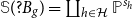 $\mathbb{S}(?B_g) = \coprod _{h \in \mathcal{H}} \mathbb{P}^{s_h}$
. Then there exists a graded
$\mathbb{S}(?B_g) = \coprod _{h \in \mathcal{H}} \mathbb{P}^{s_h}$
. Then there exists a graded
 $\mathbb{k}$
-algebra
$\mathbb{k}$
-algebra
 $S$
, such that for each Hilbert function
$S$
, such that for each Hilbert function
 $h \in \mathcal{H}$
, there is a fixed choice of closed immersion
$h \in \mathcal{H}$
, there is a fixed choice of closed immersion
 $H_S^h \longrightarrow \mathbb{P}^{s_h}$
. We set
$H_S^h \longrightarrow \mathbb{P}^{s_h}$
. We set
 $\mathbb{Y}(\pi ') = \coprod _{h \in \mathcal{H}}H_S^{h_s} \cap \mathbb{S}(\pi ')$
.
$\mathbb{Y}(\pi ') = \coprod _{h \in \mathcal{H}}H_S^{h_s} \cap \mathbb{S}(\pi ')$
.
For the edges
 $e$
of
$e$
of
 $\pi '$
displayed in (
91
), define a morphism
$\pi '$
displayed in (
91
), define a morphism
 $\rho _e$
to be a projection according to the following table:
$\rho _e$
to be a projection according to the following table:
| Edge label |
 $\rho _e$
|
|---|---|
 $\neg A_h$
|
 $\mathbb{S}(\pi ) \longrightarrow \mathbb{S}(\neg A_a)$
|
 $A_i$
$A_i$
|
 $\mathbb{S}(\pi ) \longrightarrow \mathbb{S}(A_b)$
|
 $?B_j$
|
 $\mathbb{S}(\pi ) \longrightarrow \mathbb{S}(?B_c)$
|

For every edge
 $e$
of
$e$
of
 $\pi '$
which is not displayed in (
96
), there is a corresponding edge
$\pi '$
which is not displayed in (
96
), there is a corresponding edge
 $e'$
of
$e'$
of
 $\pi$
. For these, we set
$\pi$
. For these, we set
 $\rho _e$
to be the projection
$\rho _e$
to be the projection
 $\mathbb{S}(\pi ) \longrightarrow \mathbb{S}(A_{e'})$
. We define
$\mathbb{S}(\pi ) \longrightarrow \mathbb{S}(A_{e'})$
. We define
 $S_{\gamma }: \mathbb{S}(\pi ) \longrightarrow \mathbb{S}(\pi ')$
to be the morphism given by the universal property of the product and the set
$S_{\gamma }: \mathbb{S}(\pi ) \longrightarrow \mathbb{S}(\pi ')$
to be the morphism given by the universal property of the product and the set
 $\{\rho _e\}_{e \in \mathcal{E}_{\pi '}}$
.
$\{\rho _e\}_{e \in \mathcal{E}_{\pi '}}$
.
For the following edges
 $e$
of
$e$
of
 $\pi$
displayed in (
96
), we define a morphism
$\pi$
displayed in (
96
), we define a morphism
 $\tau _e$
to be a projection according to the following table:
$\tau _e$
to be a projection according to the following table:
| Edge label |
 $\tau _e$
|
|---|---|
 $\neg A_a$
|
 $\mathbb{S}(\pi ') \longrightarrow \mathbb{S}(\neg A_h)$
|
 $A_b$
$A_b$
|
 $\mathbb{S}(\pi ') \longrightarrow \mathbb{S}(A_i)$
|
 $?B_c$
|
 $\mathbb{S}(\pi ') \longrightarrow \mathbb{S}(?B_j)$
|
 $?B_g$
|
 $\mathbb{S}(\pi ') \longrightarrow \mathbb{S}(?B_j)$
|

Let
 $\zeta$
denote the proof net in the interior of the displayed box. We have already seen in Definition 3.0.4 that if
$\zeta$
denote the proof net in the interior of the displayed box. We have already seen in Definition 3.0.4 that if
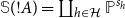 $\mathbb{S}(!A) = \coprod _{h \in \mathcal{H}}\mathbb{P}^{s_h}$
and if we are given an element
$\mathbb{S}(!A) = \coprod _{h \in \mathcal{H}}\mathbb{P}^{s_h}$
and if we are given an element
 $h_1 \in \mathcal{H}$
, we can construct graded
$h_1 \in \mathcal{H}$
, we can construct graded
 $\mathbb{k}$
-algebras
$\mathbb{k}$
-algebras
 $S_1, S$
along with a morphism
$S_1, S$
along with a morphism
 \begin{align} f: H_{S_1}^{h_1} \longrightarrow H_S^h \end{align}
as in ( 70 ). We post-compose with the canonical inclusion to obtain
 \begin{align} H_{S_1}^{h_1} \longrightarrow \coprod _{h \in \mathcal{H}} H_S^h \cong \mathbb{S}(!A). \end{align}
By the universal property of the disjoint union, we obtain
 \begin{align} \coprod _{h_1 \in \mathcal{H}}H_{S_1}^{h_1} \longrightarrow \mathbb{S}(!A) \end{align}
which we pre-compose with
 $(\phi _{\operatorname {P}^2}\vert _{\coprod _{h_1 \in \mathcal{H}}H_{S_1}^{h_1}})^{-1}$
, which is the inverse of a restriction of
$(\phi _{\operatorname {P}^2}\vert _{\coprod _{h_1 \in \mathcal{H}}H_{S_1}^{h_1}})^{-1}$
, which is the inverse of a restriction of
 $\phi _{\operatorname {P}^2}$
of Definition 3.0.4 in order to obtain
$\phi _{\operatorname {P}^2}$
of Definition 3.0.4 in order to obtain
 \begin{equation} \coprod _{h_1 \in \mathcal{H}}H_{S_1}^{h_1} \cap (\mathbb{S}(?B_j) \times \mathbb{S}(A_i)) \longrightarrow \mathbb{S}(!A). \end{equation}
We take
 $\tau _e$
, for
$\tau _e$
, for
 $e$
the edges labelled
$e$
the edges labelled
 $!A_f, ?\neg A_d$
, to be the result of pre-composing this with (the restriction of) the projection
$!A_f, ?\neg A_d$
, to be the result of pre-composing this with (the restriction of) the projection
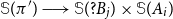 $\mathbb{S}(\pi ') \longrightarrow \mathbb{S}(?B_j) \times \mathbb{S}(A_i)$
:
$\mathbb{S}(\pi ') \longrightarrow \mathbb{S}(?B_j) \times \mathbb{S}(A_i)$
:
 \begin{equation} \tau _e: \mathbb{Y}(\pi ') \longrightarrow \mathbb{S}(!A). \end{equation}
We define
 $T_\gamma : \mathbb{Y}(\pi ') \longrightarrow \mathbb{S}(\pi )$
to be the morphism induced by the universal property of the product and the set
$T_\gamma : \mathbb{Y}(\pi ') \longrightarrow \mathbb{S}(\pi )$
to be the morphism induced by the universal property of the product and the set
 $\{\tau _e\}_{e \in \mathcal{E}_{\pi }}$
.
$\{\tau _e\}_{e \in \mathcal{E}_{\pi }}$
.
 $\gamma : \pi \longrightarrow \pi '$
is a
$\gamma : \pi \longrightarrow \pi '$
is a
 $\operatorname {Weak}/!$
-reduction.
$\operatorname {Weak}/!$
-reduction.

Let
 $\varnothing _g \longrightarrow \mathbb{S}(?B_g)$
denote the empty subscheme. We set
$\varnothing _g \longrightarrow \mathbb{S}(?B_g)$
denote the empty subscheme. We set
 $\mathbb{Y}(\pi ') = \varnothing _g \cap \mathbb{S}(\pi ')$
.
$\mathbb{Y}(\pi ') = \varnothing _g \cap \mathbb{S}(\pi ')$
.
For the edge
 $e$
of (
102
) labelled
$e$
of (
102
) labelled
 $?B_g$
, define
$?B_g$
, define
 $\rho _e$
to be the projection
$\rho _e$
to be the projection
 $\rho _e: \mathbb{S}(\pi ) \longrightarrow \mathbb{S}(?B_f)$
. For every edge
$\rho _e: \mathbb{S}(\pi ) \longrightarrow \mathbb{S}(?B_f)$
. For every edge
 $e$
of
$e$
of
 $\pi '$
which is not displayed in (
96
), there is a corresponding edge
$\pi '$
which is not displayed in (
96
), there is a corresponding edge
 $e'$
of
$e'$
of
 $\pi$
. For these, we set
$\pi$
. For these, we set
 $\rho _e$
to be the projection
$\rho _e$
to be the projection
 $\mathbb{S}(\pi ) \longrightarrow \mathbb{S}(A_{e'})$
. We define
$\mathbb{S}(\pi ) \longrightarrow \mathbb{S}(A_{e'})$
. We define
 $S_{\gamma }: \mathbb{S}(\pi ) \longrightarrow \mathbb{S}(\pi ')$
to be the morphism induced by the universal property of the product and the set
$S_{\gamma }: \mathbb{S}(\pi ) \longrightarrow \mathbb{S}(\pi ')$
to be the morphism induced by the universal property of the product and the set
 $\{\rho _e\}_{e \in \mathcal{E}_{\pi '}}$
.
$\{\rho _e\}_{e \in \mathcal{E}_{\pi '}}$
.
Let
 $\zeta$
denote the proof inside the box. The empty scheme
$\zeta$
denote the proof inside the box. The empty scheme
 $\varnothing _g$
is the initial object in the category of schemes over
$\varnothing _g$
is the initial object in the category of schemes over
 $\mathbb{k}$
. For each edge
$\mathbb{k}$
. For each edge
 $e$
of
$e$
of
 $\zeta$
, we define
$\zeta$
, we define
 $\tau _{e}$
to be the unique morphism
$\tau _{e}$
to be the unique morphism
 $\tau _e: \varnothing _g \longrightarrow \mathbb{S}(A_{e})$
. If
$\tau _e: \varnothing _g \longrightarrow \mathbb{S}(A_{e})$
. If
 $e$
is labelled
$e$
is labelled
 $?\neg A_a$
or
$?\neg A_a$
or
 $!A_b$
, we similarly define
$!A_b$
, we similarly define
 $\tau _e$
to be the unique morphism
$\tau _e$
to be the unique morphism
 $\tau _e: \varnothing _g \longrightarrow \mathbb{S}(A_{e})$
. For every edge
$\tau _e: \varnothing _g \longrightarrow \mathbb{S}(A_{e})$
. For every edge
 $e$
of
$e$
of
 $\pi$
which is not displayed in (
102
), there is a corresponding edge
$\pi$
which is not displayed in (
102
), there is a corresponding edge
 $e'$
of
$e'$
of
 $\pi '$
. For these, we set
$\pi '$
. For these, we set
 $\tau _e$
to be the projection
$\tau _e$
to be the projection
 $\tau _e: \mathbb{S}(\pi ') \longrightarrow \mathbb{S}(A_{e'})$
. We define
$\tau _e: \mathbb{S}(\pi ') \longrightarrow \mathbb{S}(A_{e'})$
. We define
 $T_\gamma : \mathbb{Y}(\pi ') \longrightarrow \mathbb{S}(\pi )$
to be the morphism induced by the universal property of the product and the set
$T_\gamma : \mathbb{Y}(\pi ') \longrightarrow \mathbb{S}(\pi )$
to be the morphism induced by the universal property of the product and the set
 $\{\tau _e\}_{e \in \mathcal{E}_\pi }$
.
$\{\tau _e\}_{e \in \mathcal{E}_\pi }$
.
 $\gamma : \pi \longrightarrow \pi '$
is a
$\gamma : \pi \longrightarrow \pi '$
is a
 $\operatorname {Ctr}/!$
-reduction.
Set
$\operatorname {Ctr}/!$
-reduction.
Set
 $\mathbb{Y}(\pi ') = \mathbb{S}(\pi ')$
.
$\mathbb{Y}(\pi ') = \mathbb{S}(\pi ')$
.

For the edges
 $e$
of
$e$
of
 $\pi '$
displayed in (
103
), define a morphism
$\pi '$
displayed in (
103
), define a morphism
 $\rho _e$
to be a projection according to the following table:
$\rho _e$
to be a projection according to the following table:
| Edge label |
 $\rho _e$
|
|---|---|
 $?\neg A_m$
|
 $\mathbb{S}(\pi ) \longrightarrow \mathbb{S}(?A_g)$
|
 $!A_n$
|
 $\mathbb{S}(\pi ) \longrightarrow \mathbb{S}(!A_g)$
|
 $A_i$
$A_i$
|
 $\mathbb{S}(\pi ) \longrightarrow \mathbb{S}(A_c)$
|
 $?B_j$
|
 $\mathbb{S}(\pi ) \longrightarrow \mathbb{S}(?B_d)$
|
 $?B_o$
|
 $\mathbb{S}(\pi ) \longrightarrow \mathbb{S}(?B_h)$
|
 $?\neg A_p$
|
 $\mathbb{S}(\pi ) \longrightarrow \mathbb{S}(?\neg A_g)$
|
 $!A_q$
|
 $\mathbb{S}(\pi ) \longrightarrow \mathbb{S}(!A_g)$
|
 $A_k$
$A_k$
|
 $\mathbb{S}(\pi ) \longrightarrow \mathbb{S}(A_c)$
|
 $?B_l$
|
 $\mathbb{S}(\pi ) \longrightarrow \mathbb{S}(?B_d)$
|
 $?B_r$
|
 $\mathbb{S}(\pi ) \longrightarrow \mathbb{S}(?B_h)$
|
 $?B_s$
|
 $\mathbb{S}(\pi ) \longrightarrow \mathbb{S}(?B_h)$
|

For every edge
 $e$
of
$e$
of
 $\pi '$
which is not displayed in (
103
), there is a corresponding edge
$\pi '$
which is not displayed in (
103
), there is a corresponding edge
 $e'$
of
$e'$
of
 $\pi$
. For these, we set
$\pi$
. For these, we set
 $\rho _e$
to be the projection
$\rho _e$
to be the projection
 $\rho _e: \mathbb{S}(\pi ) \longrightarrow \mathbb{S}(A_{e'})$
. We define
$\rho _e: \mathbb{S}(\pi ) \longrightarrow \mathbb{S}(A_{e'})$
. We define
 $S_{\gamma }: \mathbb{S}(\pi ) \longrightarrow \mathbb{S}(\pi ')$
to be the morphism induced by the universal property of the product and the set
$S_{\gamma }: \mathbb{S}(\pi ) \longrightarrow \mathbb{S}(\pi ')$
to be the morphism induced by the universal property of the product and the set
 $\{\rho _e\}_{e \in \mathcal{E}_{\pi '}}$
.
$\{\rho _e\}_{e \in \mathcal{E}_{\pi '}}$
.
For the edges
 $e$
of
$e$
of
 $\pi '$
displayed in (
103
), we define a morphism
$\pi '$
displayed in (
103
), we define a morphism
 $\tau _e$
to be a projection according to the following table:
$\tau _e$
to be a projection according to the following table:
| Edge label |
 $\tau _e$
|
|---|---|
 $?A_a$
|
 $\mathbb{S}(\pi ') \longrightarrow \mathbb{S}(?A_n)$
|
 $?\neg A_b$
|
 $\mathbb{S}(\pi ') \longrightarrow \mathbb{S}(!A_n)$
|
 $A_c$
$A_c$
|
 $\mathbb{S}(\pi ') \longrightarrow \mathbb{S}(A_i)$
|
 $?B_d$
|
 $\mathbb{S}(\pi ') \longrightarrow \mathbb{S}(?B_j)$
|
 $?\neg A_f$
|
 $\mathbb{S}(\pi ') \longrightarrow \mathbb{S}(?A_n)$
|
 $!A_g$
|
 $\mathbb{S}(\pi ') \longrightarrow \mathbb{S}(!A_n)$
|
 $?B_h$
|
 $\mathbb{S}(\pi ') \longrightarrow \mathbb{S}(?B_o)$
|

For every edge
 $e$
of
$e$
of
 $\pi$
which is not displayed in (
103
), there is a corresponding edge
$\pi$
which is not displayed in (
103
), there is a corresponding edge
 $e'$
of
$e'$
of
 $\pi '$
. For these, we set
$\pi '$
. For these, we set
 $\tau _e$
to be the projection
$\tau _e$
to be the projection
 $\tau _e: \mathbb{S}(\pi ') \longrightarrow \mathbb{S}(A_{e'})$
. We define
$\tau _e: \mathbb{S}(\pi ') \longrightarrow \mathbb{S}(A_{e'})$
. We define
 $T_\gamma : \mathbb{Y}(\pi ') \longrightarrow \mathbb{S}(\pi )$
to be the morphism induced by the universal property of the product and the set
$T_\gamma : \mathbb{Y}(\pi ') \longrightarrow \mathbb{S}(\pi )$
to be the morphism induced by the universal property of the product and the set
 $\{\rho _e\}_{e \in \mathcal{E}_\pi }$
.
$\{\rho _e\}_{e \in \mathcal{E}_\pi }$
.
Remark 3.1.2. We only needed to introduce the restriction
 $\mathbb{S}(\pi ')\vert _{\mathbb{Y}(\pi ')}$
in Definition 3.1.1 for
$\mathbb{S}(\pi ')\vert _{\mathbb{Y}(\pi ')}$
in Definition 3.1.1 for
 $!/?$
-reductions and
$!/?$
-reductions and
 $!/\operatorname {Weak}$
-reductions. It can be checked easily that given a reduction
$!/\operatorname {Weak}$
-reductions. It can be checked easily that given a reduction
 $\pi \stackrel {\gamma }{\longrightarrow } \pi '$
, we have
$\pi \stackrel {\gamma }{\longrightarrow } \pi '$
, we have
 \begin{equation} T_{\gamma }^{-1}(\mathbb{Y}(\pi )) \subseteq \mathbb{Y}(\pi ') \end{equation}
so that for every sequence of reductions
 \begin{equation} \pi _1 \stackrel {\gamma _1}{\longrightarrow } \ldots \stackrel {\gamma _{n-1}}{\longrightarrow } \pi _{n-1} \end{equation}
the morphisms
 $T_{\gamma _i}$
factor through the appropriate restrictions so that we end up with a composable sequence of morphisms
$T_{\gamma _i}$
factor through the appropriate restrictions so that we end up with a composable sequence of morphisms
 \begin{equation} T_{\gamma _1} \circ \ldots \circ T_{\gamma _{n-1}}. \end{equation}
Theorem 3.1.3. If
 $\gamma : \pi \longrightarrow \pi '$
is a reduction, then the morphisms
$\gamma : \pi \longrightarrow \pi '$
is a reduction, then the morphisms
 $S_{\gamma }: \mathbb{S}(\pi ) \longrightarrow \mathbb{S}(\pi '), T_{\gamma }: \mathbb{Y}(\pi ') \longrightarrow \mathbb{S}(\pi )$
restrict to well defined morphisms
$S_{\gamma }: \mathbb{S}(\pi ) \longrightarrow \mathbb{S}(\pi '), T_{\gamma }: \mathbb{Y}(\pi ') \longrightarrow \mathbb{S}(\pi )$
restrict to well defined morphisms
 \begin{align*} S_{\gamma }\vert _{\mathbb{X}(\pi )}: \mathbb{X}(\pi ) &\longrightarrow \mathbb{X}(\pi ')\\ T_{\gamma }\vert _{\mathbb{X}(\pi ')}: \mathbb{X}(\pi ') &\longrightarrow \mathbb{X}(\pi ) \end{align*}
which are mutually inverse isomorphisms.
Proof.
 $\gamma : \pi \longrightarrow \pi '$
is an
$\gamma : \pi \longrightarrow \pi '$
is an
 $\operatorname {Ax}/\operatorname {Cut}$
-reduction. We refer to Diagram (90) and consider only this type of
$\operatorname {Ax}/\operatorname {Cut}$
-reduction. We refer to Diagram (90) and consider only this type of
 $\operatorname {Ax}/\operatorname {Cut}$
-reduction.
$\operatorname {Ax}/\operatorname {Cut}$
-reduction.
It suffices to consider only the links involved in the reduction. Let
 $l$
denote the link in
$l$
denote the link in
 $\pi$
to which
$\pi$
to which
 $\neg A_c$
is the conclusion, and let
$\neg A_c$
is the conclusion, and let
 $l'$
denote the link in
$l'$
denote the link in
 $\pi$
to which
$\pi$
to which
 $\neg A_a$
is the premise. We define the following restrictions
$\neg A_a$
is the premise. We define the following restrictions
 \begin{align*} S_{\gamma , l} &= S_{\gamma }\vert _{\Delta _{a,b} \cap \Delta _{b,c} \cap \mathbb{X}(l)}\\ S_{\gamma , l'} &= S_\gamma \vert _{\mathbb{X}(l') \cap \Delta _{a,b} \cap \Delta _{b,c}} \end{align*}
and consider the following three dimensional diagram, ignoring the dashed line for now:

The morphisms
 $S_{\gamma , l}$
and
$S_{\gamma , l}$
and
 $S_{\gamma , l'}$
are isomorphisms with inverses given by
$S_{\gamma , l'}$
are isomorphisms with inverses given by
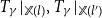 $T_\gamma \vert _{\mathbb{X}(l)}, T_{\gamma }\vert _{\mathbb{X}(l')}$
, respectively. The front-face and the back-face of the cube (107), given as follows, are both pullback diagrams:
$T_\gamma \vert _{\mathbb{X}(l)}, T_{\gamma }\vert _{\mathbb{X}(l')}$
, respectively. The front-face and the back-face of the cube (107), given as follows, are both pullback diagrams:
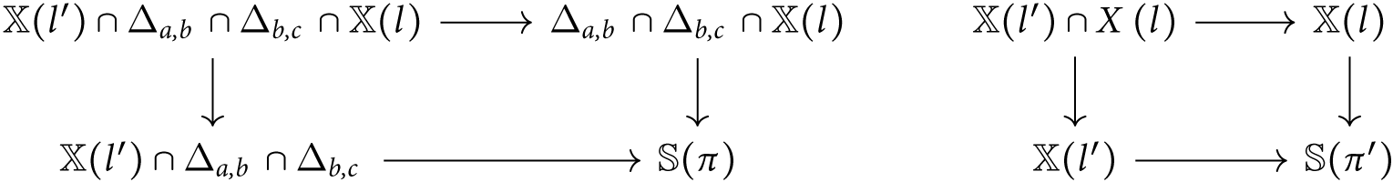
This implies that the dashed arrow
 $\mathbb{X}(l') \cap \Delta _{a,b} \cap \Delta _{b,c} \cap \mathbb{X}(l) \longrightarrow \mathbb{X}(l') \cap \mathbb{X}(l)$
in (107) exists, and is an isomorphism with inverse given by
$\mathbb{X}(l') \cap \Delta _{a,b} \cap \Delta _{b,c} \cap \mathbb{X}(l) \longrightarrow \mathbb{X}(l') \cap \mathbb{X}(l)$
in (107) exists, and is an isomorphism with inverse given by
 $T_{\gamma }\vert _{\mathbb{X}(l') \cap \mathbb{X}(l)}$
.
$T_{\gamma }\vert _{\mathbb{X}(l') \cap \mathbb{X}(l)}$
.
 $\gamma : \pi \longrightarrow \pi '$
is a
$\gamma : \pi \longrightarrow \pi '$
is a
 $\otimes / \unicode{x214B}$
-reduction. This case is similar to the previous so we omit the proof.
$\otimes / \unicode{x214B}$
-reduction. This case is similar to the previous so we omit the proof.
 $\gamma : \pi \longrightarrow \pi '$
is a
$\gamma : \pi \longrightarrow \pi '$
is a
 $!/?$
-reduction. We consider only the case where there is a restricted amount of Pax-links, and with Conclusion-links as displayed in Definition 3.1.1, but the general result follows easily from this.
$!/?$
-reduction. We consider only the case where there is a restricted amount of Pax-links, and with Conclusion-links as displayed in Definition 3.1.1, but the general result follows easily from this.
We refer to Diagram (96). Let
 $\zeta$
denote the proof net inside the box. We have already seen in Definition 3.0.4 that if we write
$\zeta$
denote the proof net inside the box. We have already seen in Definition 3.0.4 that if we write
 $\mathbb{S}(?B) = \coprod _{h \in \mathcal{H}} \mathbb{P}^{s_h}$
, fix a Hilbert function
$\mathbb{S}(?B) = \coprod _{h \in \mathcal{H}} \mathbb{P}^{s_h}$
, fix a Hilbert function
 $h_1 \in \mathcal{H}$
, denote the number of unoriented atoms of
$h_1 \in \mathcal{H}$
, denote the number of unoriented atoms of
 $B$
by
$B$
by
 $m_1$
, denote the number of unoriented atoms of
$m_1$
, denote the number of unoriented atoms of
 $A$
by
$A$
by
 $m$
, and let
$m$
, and let
 \begin{equation} S_1 = \mathbb{k}[x_0, \ldots , x_{2^{m_1}-1}],\quad S = \mathbb{k}[x_1, \ldots , x_{2^m - 1}], \end{equation}
then we can construct a morphism
 \begin{equation} f: H_{S_1}^{h_1} \longrightarrow H_S^h \end{equation}
for some Hilbert function
 $h$
. We have also shown in Definition 3.0.4 how to construct a morphism
$h$
. We have also shown in Definition 3.0.4 how to construct a morphism
 $\mathbb{U}_h \longrightarrow H_S^h \times \mathbb{S}(A)$
which we post-compose with the product of the composite
$\mathbb{U}_h \longrightarrow H_S^h \times \mathbb{S}(A)$
which we post-compose with the product of the composite
 $H_S^h \longrightarrow \mathbb{P}^{s_h} \longrightarrow \mathbb{S}(!A)$
and the identity on
$H_S^h \longrightarrow \mathbb{P}^{s_h} \longrightarrow \mathbb{S}(!A)$
and the identity on
 $\mathbb{S}(A)$
to obtain
$\mathbb{S}(A)$
to obtain
 $\iota _h: \mathbb{U}_h \longrightarrow \mathbb{S}(!A) \times \mathbb{S}(A)$
. On the other hand, consider the closed immersion
$\iota _h: \mathbb{U}_h \longrightarrow \mathbb{S}(!A) \times \mathbb{S}(A)$
. On the other hand, consider the closed immersion
 \begin{equation} \Gamma _f \longrightarrow H_{S_1}^{h_1} \times H_S^h \end{equation}
of the graph
 $\Gamma _f$
of
$\Gamma _f$
of
 $f$
. Associated to
$f$
. Associated to
 $h_1, h$
are fixed choices of closed immersions
$h_1, h$
are fixed choices of closed immersions
 $H_{S_1}^{h_1} \longrightarrow \mathbb{P}^{s_{h_1}}, H_S^h \longrightarrow \mathbb{P}^{s_h}$
which we can post-compose with the canonical inclusions to obtain
$H_{S_1}^{h_1} \longrightarrow \mathbb{P}^{s_{h_1}}, H_S^h \longrightarrow \mathbb{P}^{s_h}$
which we can post-compose with the canonical inclusions to obtain
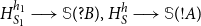 $H_{S_1}^{h_1} \longrightarrow \mathbb{S}(?B), H_S^h \longrightarrow \mathbb{S}(!A)$
. Post-composing (110) with the product of these yields
$H_{S_1}^{h_1} \longrightarrow \mathbb{S}(?B), H_S^h \longrightarrow \mathbb{S}(!A)$
. Post-composing (110) with the product of these yields
 \begin{equation} o: \Gamma _f \longrightarrow \mathbb{S}(?B) \times \mathbb{S}(!A). \end{equation}
Denote by
 $\rho : \mathbb{S}(\zeta ) \longrightarrow \mathbb{S}(?B) \times \mathbb{S}(A)$
the canonical projection and
$\rho : \mathbb{S}(\zeta ) \longrightarrow \mathbb{S}(?B) \times \mathbb{S}(A)$
the canonical projection and
 $\rho _\ast$
the pushforward. We claim that the following is a pullback diagram:
$\rho _\ast$
the pushforward. We claim that the following is a pullback diagram:

It suffices to show that the following is a pullback diagram:
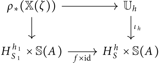
This can be shown by taking open affine charts of
 $H_{S_1}^{h_1}, H_S^h$
and using the fact that the tensor product induces pullbacks in the category
$H_{S_1}^{h_1}, H_S^h$
and using the fact that the tensor product induces pullbacks in the category
 $\mathbb{k}-\underline {\operatorname {Alg}}$
of
$\mathbb{k}-\underline {\operatorname {Alg}}$
of
 $\mathbb{k}$
-algebras.
$\mathbb{k}$
-algebras.
 $\gamma : \pi \longrightarrow \pi '$
is a
$\gamma : \pi \longrightarrow \pi '$
is a
 $\operatorname {Weak}/!$
-reduction. This case is trivial as we are mapping empty schemes to empty schemes via morphisms uniquely defined by the property that their domain is the initial object in the category of schemes over
$\operatorname {Weak}/!$
-reduction. This case is trivial as we are mapping empty schemes to empty schemes via morphisms uniquely defined by the property that their domain is the initial object in the category of schemes over
 $\mathbb{k}$
.
$\mathbb{k}$
.
 $\gamma : \pi \longrightarrow \pi '$
is a
$\gamma : \pi \longrightarrow \pi '$
is a
 $\operatorname {Ctr}/!$
-reduction. We refer to Diagram (103). Due to the diagonals at the Axiom- and Cut-links, it suffices to consider only the displayed Promotion-links, Pax-links and the displayed Contraction-link of
$\operatorname {Ctr}/!$
-reduction. We refer to Diagram (103). Due to the diagonals at the Axiom- and Cut-links, it suffices to consider only the displayed Promotion-links, Pax-links and the displayed Contraction-link of
 $\pi '$
.
$\pi '$
.
Let
 $l_!, l_{\operatorname {Pax}}$
respectively denote the displayed Promotion and Pax-links of
$l_!, l_{\operatorname {Pax}}$
respectively denote the displayed Promotion and Pax-links of
 $\pi$
. Let
$\pi$
. Let
 $l_!^L$
,
$l_!^L$
,
 $l_{\operatorname {Pax}}^L$
,
$l_{\operatorname {Pax}}^L$
,
 $l_!^R$
,
$l_!^R$
,
 $L_{\operatorname {Pax}}^R$
,
$L_{\operatorname {Pax}}^R$
,
 $l_{\operatorname {Ctr}}$
, respectively, denote the Promotion-link of
$l_{\operatorname {Ctr}}$
, respectively, denote the Promotion-link of
 $\pi '$
displayed on the left, the Pax-link of
$\pi '$
displayed on the left, the Pax-link of
 $\pi '$
displayed on the left, the Promotion-link of
$\pi '$
displayed on the left, the Promotion-link of
 $\pi '$
displayed on the right, the Pax-link of
$\pi '$
displayed on the right, the Pax-link of
 $\pi '$
displayed on the right, and the Contraction-link of
$\pi '$
displayed on the right, and the Contraction-link of
 $\pi '$
.
$\pi '$
.
By inspection of the definition of
 $S_\gamma , T_\gamma$
, we obtain the following commuting diagram
$S_\gamma , T_\gamma$
, we obtain the following commuting diagram
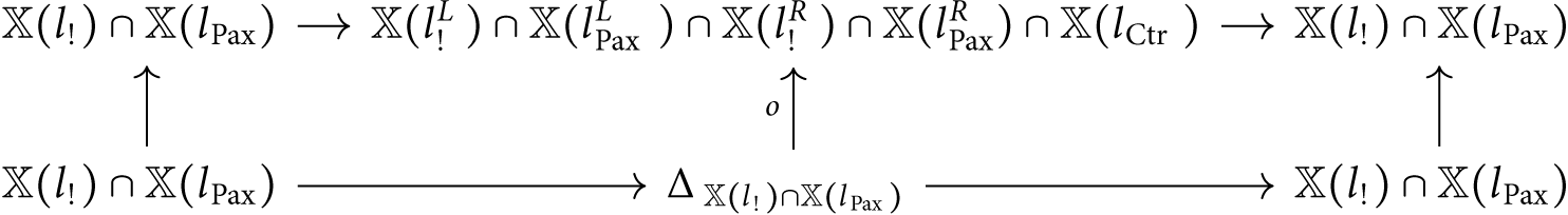
where
 \begin{equation} \Delta _{\mathbb{X}(l_!) \cap \mathbb{X}(l_{\operatorname {Pax}})} \longrightarrow \big (\mathbb{S}(A_c) \times \mathbb{S}(?B_d) \times \mathbb{S}(!A_g) \times \mathbb{S}(?B_h)\big )^2 \end{equation}
denotes the diagonal which factors through
 $o$
. All vertical arrows are isomorphisms, and the bottom horizontal composition is the identity. The argument for the other composite is similar.
$o$
. All vertical arrows are isomorphisms, and the bottom horizontal composition is the identity. The argument for the other composite is similar.
3.2 An example
The Church numerals provide an interesting class of shallow proofs. It was explained in the Introduction how the exponential fragment of linear logic provides equations
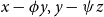 $x - \phi y, y - \psi z$
, for example. In this setting, the Church numeral
$x - \phi y, y - \psi z$
, for example. In this setting, the Church numeral
 $\underline {2}_X$
(for
$\underline {2}_X$
(for
 $X$
an atomic formula) will give rise to these exact equations once appropriate localisations have been chosen. Moreover, we obtain the equation
$X$
an atomic formula) will give rise to these exact equations once appropriate localisations have been chosen. Moreover, we obtain the equation
 $\phi - \psi$
. A consequence of setting these equations to zero is that
$\phi - \psi$
. A consequence of setting these equations to zero is that
 $x = \phi ^2 z$
, where the power of 2 reflects the fact that we took the Church numeral two. Indeed, the Church numeral
$x = \phi ^2 z$
, where the power of 2 reflects the fact that we took the Church numeral two. Indeed, the Church numeral
 $\underline {n}_X$
gives rise to the equation
$\underline {n}_X$
gives rise to the equation
 $x = \phi ^n z$
.
$x = \phi ^n z$
.
3.2.1 Cutting
$\underline{2}_X$
against
$\underline{0}_X$


Consider the following proof net
 $\pi$
, which is the Church numeral
$\pi$
, which is the Church numeral
 $\underline {2}_X$
cut against a simple proof net given by appending a Promotion-link to the Church numeral
$\underline {2}_X$
cut against a simple proof net given by appending a Promotion-link to the Church numeral
 $\underline {0}_X$
. We have labelled the formulas artificially; each
$\underline {0}_X$
. We have labelled the formulas artificially; each
 $X_p$
means the atomic formula
$X_p$
means the atomic formula
 $X$
.
$X$
.
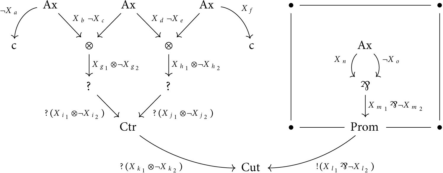
Associated to the Axiom-links are the following projective schemes:
 \begin{equation*} \mathbb{S}(\neg X_a) = \mathbb{S}(X_b) = \mathbb{S}(\neg X_c) = \mathbb{S}(X_d) = \mathbb{S}(\neg X_e) = \mathbb{S}(X_f) = \mathbb{S}(X_n) = \mathbb{S}(\neg X_o) = \mathbb{P}^1. \end{equation*}
For the Tensor- and Par-links, we should be considering the Segre embedding
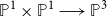 $\mathbb{P}^1 \times \mathbb{P}^1 \longrightarrow \mathbb{P}^3$
, so that the interpretation of each non-atomic linear formula of
$\mathbb{P}^1 \times \mathbb{P}^1 \longrightarrow \mathbb{P}^3$
, so that the interpretation of each non-atomic linear formula of
 $\pi$
is
$\pi$
is
 $\mathbb{P}^3$
but to make the ideas of the model more transparent within this example, we will directly consider the closed subscheme
$\mathbb{P}^3$
but to make the ideas of the model more transparent within this example, we will directly consider the closed subscheme
 $\mathbb{P}^1 \times \mathbb{P}^1$
:
$\mathbb{P}^1 \times \mathbb{P}^1$
:
 \begin{equation*} \mathbb{S}(X_{g_1} \otimes \neg X_{g_2}) = \mathbb{S}(X_{h_1} \otimes \neg X_{h_2}) = \mathbb{S}(X_{m_1} \unicode{x214B} \neg X_{m_2}) = \mathbb{P}^1 \times \mathbb{P}^1. \end{equation*}
For each of the linear formulas, we consider a corresponding graded
 $\mathbb{k}$
-algebra. For instance, associated to the formula
$\mathbb{k}$
-algebra. For instance, associated to the formula
 $\neg X_a$
is the graded
$\neg X_a$
is the graded
 $\mathbb{k}$
-algebra
$\mathbb{k}$
-algebra
 $\mathbb{k}[X_a', X_a]$
. Since the variable
$\mathbb{k}[X_a', X_a]$
. Since the variable
 $X$
is consistent throughout all of the formulas, we will use the algebra
$X$
is consistent throughout all of the formulas, we will use the algebra
 $\mathbb{k}[a',a]$
in place of
$\mathbb{k}[a',a]$
in place of
 $\mathbb{k}[X_a', X_a]$
, and similarly for the other variables.
$\mathbb{k}[X_a', X_a]$
, and similarly for the other variables.
Let
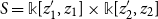 $S = \mathbb{k}[z_1', z_1] \times \mathbb{k}[z_2', z_2]$
. Then for each Hilbert function
$S = \mathbb{k}[z_1', z_1] \times \mathbb{k}[z_2', z_2]$
. Then for each Hilbert function
 $h \in \mathcal{H}$
, we have a fixed choice of closed immersion of the Hilbert scheme
$h \in \mathcal{H}$
, we have a fixed choice of closed immersion of the Hilbert scheme
 $H_S^h$
given by Proposition 2.3.27 into some projective space
$H_S^h$
given by Proposition 2.3.27 into some projective space
 $\mathbb{P}^{s_h}$
. We take the disjoint union of the codomains of these:
$\mathbb{P}^{s_h}$
. We take the disjoint union of the codomains of these:
 \begin{align*} \mathbb{S}(?(X_{i_1} \otimes \neg X_{i_2})) &= \mathbb{S}(?(X_{j_1} \otimes \neg X_{j_2}))\\ = \mathbb{S}(?(X_{k_1} \otimes \neg X_{k_2})) &= \mathbb{S}(!(X_{l_1} \otimes \neg X_{l_2})) = \coprod _{h \in \mathcal{H}}\mathbb{P}^{s_h}. \end{align*}
The interior of the box of
 $\pi$
determines a point in
$\pi$
determines a point in
 $\coprod _{h \in \mathcal{H}}\mathbb{P}^{s_h}$
, which is inside the closed subscheme
$\coprod _{h \in \mathcal{H}}\mathbb{P}^{s_h}$
, which is inside the closed subscheme
 $H_S^{h^\ast } \subseteq \mathbb{P}^{s_h}$
for some particular Hilbert function
$H_S^{h^\ast } \subseteq \mathbb{P}^{s_h}$
for some particular Hilbert function
 $h^\ast$
. So, for this example, we can restrict to the particular connected component of the Hilbert scheme determined by this Hilbert function, which we now calculate.
$h^\ast$
. So, for this example, we can restrict to the particular connected component of the Hilbert scheme determined by this Hilbert function, which we now calculate.
Consider
 $\underline {0}_X$
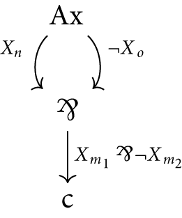
We build the closed subscheme
 $\mathbb{X}(\underline {0}_X)$
. From the Axiom-link
$\mathbb{X}(\underline {0}_X)$
. From the Axiom-link
 $l_{\operatorname {Ax}}$
, we have the diagonal
$l_{\operatorname {Ax}}$
, we have the diagonal
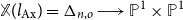 $\mathbb{X}(l_{\operatorname {Ax}}) = \Delta _{n,o} \longrightarrow \mathbb{P}^1 \times \mathbb{P}^1$
. If we consider the projection
$\mathbb{X}(l_{\operatorname {Ax}}) = \Delta _{n,o} \longrightarrow \mathbb{P}^1 \times \mathbb{P}^1$
. If we consider the projection
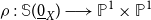 $\rho : \mathbb{S}(\underline {0}_X) \longrightarrow \mathbb{P}^1 \times \mathbb{P}^1$
, then the composite
$\rho : \mathbb{S}(\underline {0}_X) \longrightarrow \mathbb{P}^1 \times \mathbb{P}^1$
, then the composite
 \begin{equation} \mathbb{X}(\underline {0}_X) \longrightarrow \mathbb{S}(\underline {0}_X) \longrightarrow \mathbb{S}(X_{m_1} \unicode{x214B} \neg X_{m_2}) = \mathbb{P}^1 \times \mathbb{P}^1 \end{equation}
is isomorphic to the diagonal
 \begin{equation} \mathbb{P}^1 \stackrel {\Delta }{\longrightarrow } \mathbb{P}^1 \times \mathbb{P}^1. \end{equation}
The ideal
 \begin{equation} I = (m_1m_2' - m_1'm_2) \subseteq \mathbb{k}[m_1',m_1] \times _{\mathbb{k}} \mathbb{k}[m_2', m_2], \end{equation}
with
 $S = \mathbb{k}[m_1',m_1] \times _{\mathbb{k}}\mathbb{k}[m_2',m_2]$
, is such that
$S = \mathbb{k}[m_1',m_1] \times _{\mathbb{k}}\mathbb{k}[m_2',m_2]$
, is such that
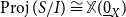 $\operatorname {Proj}(S/I) \cong \mathbb{X}(\underline {0}_X)$
(as closed subschemes of
$\operatorname {Proj}(S/I) \cong \mathbb{X}(\underline {0}_X)$
(as closed subschemes of
 $\mathbb{P}^1 \times \mathbb{P}^1$
). Conceptually, this ideal may be thought of as its corresponding counterpart obtained by dividing by the primed variables. More specifically, we have
$\mathbb{P}^1 \times \mathbb{P}^1$
). Conceptually, this ideal may be thought of as its corresponding counterpart obtained by dividing by the primed variables. More specifically, we have
 \begin{equation} \Big (\frac {m_1m_2'}{m_1'm_2'} - \frac {m_1'm_2}{m_1'm_2'}\Big ) \subseteq S_{(m_1'm_2')}. \end{equation}
Carrying this through the composition of
 $\mathbb{k}$
-algebra isomorphisms
$\mathbb{k}$
-algebra isomorphisms
 \begin{equation} S_{(m_1'm_2')} \longrightarrow \mathbb{k}[m_1/m_1',m_2/m_2'] \longrightarrow \mathbb{k}[m_1, m_2] \end{equation}
determined by the rules
 \begin{equation} \frac {m_1m_2'}{m_1'm_2'} \longmapsto m_1/m_1' \longrightarrow m_1,\quad \frac {m_1'm_2}{m_1'm_2'} \longmapsto m_2/m_2' \longrightarrow m_2 \end{equation}
we obtain the ideal
 \begin{equation} (m_1 - m_2) \subseteq \mathbb{k}[m_1, m_2]. \end{equation}
So, we can think of (116) as the equation “
 $m_1 = m_2$
,” see Section 3.3 for more details.
$m_1 = m_2$
,” see Section 3.3 for more details.
We saw in Example 2.3.25 that the Hilbert function of
 $I \subseteq S$
is
$I \subseteq S$
is
 $h^\ast (d) = 2d + 1$
, and that the Gotzmann number
$h^\ast (d) = 2d + 1$
, and that the Gotzmann number
 $G(I)$
of
$G(I)$
of
 $I$
is 2. The degree
$I$
is 2. The degree
 $2$
component of the algebra corresponding to
$2$
component of the algebra corresponding to
 $\mathbb{P}^3$
maps onto the degree
$\mathbb{P}^3$
maps onto the degree
 $1$
component of the algebra corresponding to
$1$
component of the algebra corresponding to
 $\mathbb{P}^1 \times \mathbb{P}^1$
. The Hilbert scheme
$\mathbb{P}^1 \times \mathbb{P}^1$
. The Hilbert scheme
 $H_S^{h^\ast }$
is by Proposition 2.3.27 therefore a closed subscheme of
$H_S^{h^\ast }$
is by Proposition 2.3.27 therefore a closed subscheme of
 $G_{S_{1}}^{h^\ast (1)} = G_{4}^3$
. We identify the degree
$G_{S_{1}}^{h^\ast (1)} = G_{4}^3$
. We identify the degree
 $1$
component
$1$
component
 $S_1$
of
$S_1$
of
 $S$
with
$S$
with
 $\mathbb{k}^{4}$
via the isomorphism defined by linearity and the following assignments, where
$\mathbb{k}^{4}$
via the isomorphism defined by linearity and the following assignments, where
 $e_1, \ldots , e_{4}$
are the standard basis vectors for
$e_1, \ldots , e_{4}$
are the standard basis vectors for
 $\mathbb{k}^{4}$
:
$\mathbb{k}^{4}$
:
 \begin{align} m_1'm_2' \longmapsto e_1 \quad m_1m_2' \longmapsto e_2 \quad m_1'm_2 \longmapsto e_3 \quad m_1m_2 \longmapsto e_4. \end{align}
Let
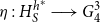 $\eta : H_S^{h^\ast } \longrightarrow G_{4}^3$
denote this closed immersion. Recall from Lemma 2.3.6 that for any size
$\eta : H_S^{h^\ast } \longrightarrow G_{4}^3$
denote this closed immersion. Recall from Lemma 2.3.6 that for any size
 $k$
subset
$k$
subset
 $B$
of
$B$
of
 $\{e_1, \ldots , e_{4}\}$
the open subset
$\{e_1, \ldots , e_{4}\}$
the open subset
 $G_{4\backslash B}^3 \subseteq G_{4}^3$
is representable. Consider the set
$G_{4\backslash B}^3 \subseteq G_{4}^3$
is representable. Consider the set
 $B = \{e_3\}$
which corresponds to
$B = \{e_3\}$
which corresponds to
 $\{m_1'm_2\} \subseteq S_1$
. There exists the following pullback diagram:
$\{m_1'm_2\} \subseteq S_1$
. There exists the following pullback diagram:
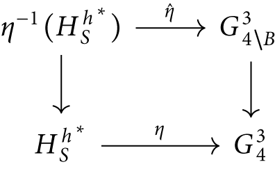
By Lemma 2.3.6,
 $G_{4\backslash B}^3$
is represented by
$G_{4\backslash B}^3$
is represented by
 $\operatorname {Spec}\mathcal{A}$
where
$\operatorname {Spec}\mathcal{A}$
where
 $\mathcal{A}$
is the following ring:
$\mathcal{A}$
is the following ring:
 \begin{equation} \mathcal{A} = \mathbb{k}[\{y_{i} \mid 1 \leq i \leq 3\}]. \end{equation}
Since
 $\eta$
is a closed immersion, it follows that
$\eta$
is a closed immersion, it follows that
 $\hat {\eta }$
is and so there exists an ideal
$\hat {\eta }$
is and so there exists an ideal
 $\mathcal{J} \subseteq S$
such that
$\mathcal{J} \subseteq S$
such that
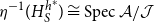 $\eta ^{-1}(H_S^{h^\ast }) \cong \operatorname {Spec}\mathcal{A}/\mathcal{J}$
. By representability of
$\eta ^{-1}(H_S^{h^\ast }) \cong \operatorname {Spec}\mathcal{A}/\mathcal{J}$
. By representability of
 $\underline {H_S^{h^\ast }}$
and
$\underline {H_S^{h^\ast }}$
and
 $\underline {G_{4}^3}$
, the morphism
$\underline {G_{4}^3}$
, the morphism
 $\eta$
corresponds to a natural transformation
$\eta$
corresponds to a natural transformation
 $\underline {\eta }$
between functors
$\underline {\eta }$
between functors
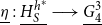 $\underline {\eta }: \underline {H_S^{h^\ast }} \longrightarrow \underline {G_{4}^3}$
. Let
$\underline {\eta }: \underline {H_S^{h^\ast }} \longrightarrow \underline {G_{4}^3}$
. Let
 $R$
be a
$R$
be a
 $\mathbb{k}$
-algebra, the function
$\mathbb{k}$
-algebra, the function
 $\underline {\eta }_R: \underline {H_S^{h^\ast }}(R) \longrightarrow \underline {G_{4}^3}(R)$
maps a homogeneous ideal
$\underline {\eta }_R: \underline {H_S^{h^\ast }}(R) \longrightarrow \underline {G_{4}^3}(R)$
maps a homogeneous ideal
 $L \subseteq R \otimes _{\mathbb{k}}S$
to the submodule
$L \subseteq R \otimes _{\mathbb{k}}S$
to the submodule
 $L_1 \subseteq R \otimes _{\mathbb{k}}S_1 \cong R^{4}$
. A homomorphism
$L_1 \subseteq R \otimes _{\mathbb{k}}S_1 \cong R^{4}$
. A homomorphism
 $\mathcal{A}/\mathcal{J} \longrightarrow R$
is given by a collection of coefficients
$\mathcal{A}/\mathcal{J} \longrightarrow R$
is given by a collection of coefficients
 $\{\alpha _{p} \in R\}_{1 \leq p \leq 3}$
satisfying the equations of
$\{\alpha _{p} \in R\}_{1 \leq p \leq 3}$
satisfying the equations of
 $\mathcal{J}$
. These equations determine the Hilbert scheme as a subscheme of the Grassmann scheme, and so, for the sake of simplicity, we can ignore them and deal only with the coefficients
$\mathcal{J}$
. These equations determine the Hilbert scheme as a subscheme of the Grassmann scheme, and so, for the sake of simplicity, we can ignore them and deal only with the coefficients
 $\{\alpha _{p} \in R\}_{1 \leq p \leq 3}$
, i.e.
$\{\alpha _{p} \in R\}_{1 \leq p \leq 3}$
, i.e.
 $\mathbb{k}$
-algebra homomorphisms
$\mathbb{k}$
-algebra homomorphisms
 $\mathcal{A} \longrightarrow R$
, i.e. points of the Grassmann scheme
$\mathcal{A} \longrightarrow R$
, i.e. points of the Grassmann scheme
 $\operatorname {Spec}R \longrightarrow G_{4\backslash B}^3$
.
$\operatorname {Spec}R \longrightarrow G_{4\backslash B}^3$
.
We have the following equation in
 $\mathcal{A}/I$
by (121).
$\mathcal{A}/I$
by (121).
 \begin{align*} m_1m_2' = m_1'm_2 \end{align*}
which corresponds to the following subspace of
 $\mathbb{k}^{4}$
:
$\mathbb{k}^{4}$
:
 \begin{equation} \operatorname {Span}_{\mathbb{k}}\{e_2 - e_3 \}. \end{equation}
So, we define a function
 $\mathcal{A} \longrightarrow \mathbb{k}$
as the
$\mathcal{A} \longrightarrow \mathbb{k}$
as the
 $\mathbb{k}$
-algebra homomorphism generated by the following rules:
$\mathbb{k}$
-algebra homomorphism generated by the following rules:
 \begin{equation} y_{1} \longmapsto 0,\quad y_2 \longmapsto 1, \quad y_3 \longmapsto 0. \end{equation}
These equations come from the fact that in
 $\mathbb{k}^4/\operatorname {Span}_{\mathbb{k}}\{e_2 - e_3 \}$
we have the equation
$\mathbb{k}^4/\operatorname {Span}_{\mathbb{k}}\{e_2 - e_3 \}$
we have the equation
 $e_3 = y_0 e_1 + y_1 e_2 + y_3 e_4$
, if
$e_3 = y_0 e_1 + y_1 e_2 + y_3 e_4$
, if
 $y_1 = y_3 = 0, y_2 = 1$
. Thus, the ideal corresponding to the Promotion-link is
$y_1 = y_3 = 0, y_2 = 1$
. Thus, the ideal corresponding to the Promotion-link is
 \begin{equation} (y_1, y_2 - 1, y_3) \subseteq \mathcal{A}. \end{equation}
Now we consider the Dereliction-link:
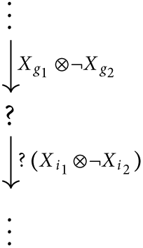
For the Hilbert function
 $h^\ast$
, we have again that
$h^\ast$
, we have again that
 $G_{4\backslash B}^3$
is represented by another copy of
$G_{4\backslash B}^3$
is represented by another copy of
 $\mathcal{A}$
:
$\mathcal{A}$
:
 \begin{equation} \mathcal{A}' = \mathbb{k}[y_{i}' \mid 1 \leq i \leq 3]. \end{equation}
There is a universal subspace of
 $(\mathcal{A}')^{4}$
with basis
$(\mathcal{A}')^{4}$
with basis
 $B$
given as follows:
$B$
given as follows:
 \begin{equation} \operatorname {Span}_{\mathcal{A}'}\{e_3 - y_1'e_1 - y_2'e_2 - y_3'e_4\} \subseteq (\mathcal{A}')^{4}. \end{equation}
This translates through (121) (with
 $m_1',m_1,m_2',m_2$
, respectively, replaced by
$m_1',m_1,m_2',m_2$
, respectively, replaced by
 $g_1',g_1,g_2',g_2$
) to
$g_1',g_1,g_2',g_2$
) to
 \begin{equation} (g_1'g_2 - y_1' g_1'g_2' - y_2' g_1g_2' - y_3' g_1g_2) \subseteq \mathcal{A}'[g_1', g_1] \times _{\mathbb{k}} \mathcal{A}'[g_2', g_2]. \end{equation}
Similarly, for the other Dereliction-link, we have a third copy of
 $\mathcal{A}$
:
$\mathcal{A}$
:
 \begin{equation} \mathcal{A}'' = \mathbb{k}[y_i'' \mid 1 \leq i \leq 3] \end{equation}
and the universal subspace
 \begin{equation} \operatorname {Span}_{\mathcal{A}''}\{e_3 - y_1''e_1 - y_2''e_2 - y_3''e_4)\} \subseteq (\mathcal{A}'')^{4} \end{equation}
with corresponding ideal
 \begin{equation} (h_1'h_2 - y_1'' h_1'h_2' - y_2'' h_1h_2' - y_3'' h_1h_2) \subseteq \mathcal{A}''[h_1', h_1] \times _{\mathbb{k}} \mathcal{A}''[h_2', h_2]. \end{equation}
The Contraction-link introduces a fourth copy of
 $\mathcal{A}$
:
$\mathcal{A}$
:
 \begin{equation} \mathcal{A}''' = \mathbb{k}[y_i''' \mid 1 \leq i \leq 3] \end{equation}
and contributes the following ideal
 \begin{equation} (y'_i - y'''_i, y''_i - y'''_i)_{1 \leq i \leq 3} \subseteq \mathcal{A}' \otimes _{\mathbb{k}} \mathcal{A}'' \otimes _{\mathbb{k}}\mathcal{A}'''. \end{equation}
Finally, the Cut-link contributes the ideal
 \begin{equation} (y'''_i - y_i)_{1 \leq i \leq 3} \subseteq \mathcal{A}''' \otimes _{\mathbb{k}} \mathcal{A}. \end{equation}
All that remains to be considered is the linear component of the proof. The Axiom-link with conclusions
 $\neg X_a, X_b$
is interpreted as the diagonal
$\neg X_a, X_b$
is interpreted as the diagonal
 $\Delta \longrightarrow \mathbb{P}^1 \times \mathbb{P}^1$
, which is given by the following ideal:
$\Delta \longrightarrow \mathbb{P}^1 \times \mathbb{P}^1$
, which is given by the following ideal:
 \begin{equation} (ab' - a'b) \subseteq \mathbb{k}[a', a] \times _{\mathbb{k}} \mathbb{k}[b',b]. \end{equation}
The other Axiom-links are treated similarly.
The Tensor-link with conclusion
 $X_{g_1} \otimes \neg X_{g_2}$
contributes the following ideal:
$X_{g_1} \otimes \neg X_{g_2}$
contributes the following ideal:
 \begin{align*} &(g_1g_2'b'c' - g_1'g_2'bc', g_1'g_2b'c' - g_1'g_2'b'c, g_1g_2b'c' - g_1'g_2'bc)\\ &\subseteq \big (\mathbb{k}[g_1',g_1] \times _{\mathbb{k}} \mathbb{k}[g_2', g_2]\big ) \times _{\mathbb{k}} \mathbb{k}[b', b] \times _{\mathbb{k}} \mathbb{k}[c',c]. \end{align*}
Again, we can think of this as the corresponding ideal given by dividing by the primed variables, given as follows:
 \begin{equation} (g_1 - b, g_2 - c, g_1g_2 - bc) = (g_1 - b, g_2 - c) \subseteq \mathbb{k}[g_1, g_2, b, c]. \end{equation}
This reflects the logical structure that the premises
 $X_b,\neg X_c$
of the Tensor-link have respective corresponding conclusions
$X_b,\neg X_c$
of the Tensor-link have respective corresponding conclusions
 $X_{g_1}, \neg X_{g_2}$
.
$X_{g_1}, \neg X_{g_2}$
.
The other Tensor-link and the Par-link are similar. We thus have the following set of equations:
 \begin{align*} ab' - a'b,\quad cd' - c'd,\quad ef'-e'f,\quad no' - n'o, \end{align*}
 \begin{align*} g_1g_2'b'c' &- g_1'g_2'bc', & g_1'g_2b'c' &- g_1'g_2'b'c, & g_1g_2b'c' &- g_1'g_2'bc,\\ h_1h_2'd'e' &- h_1'h_2'de', & h_1'h_2d'e' &- h_1'h_2' d'e, & h_1h_2d'e' &- h_1'h_2'de,\\ m_1m_2'n'o' &- m_1'm_2'no', & m_1'm_2n'o' &- m_1'm_2'n'o, & m_1m_2n'o' &- m_1'm_2'no, \end{align*}
 \begin{equation*} g_1'g_2 - y_1' g_1'g_2' - y_2' g_1g_2' - y_3' g_1g_2, \end{equation*}
 \begin{equation*} h_1'h_2 - y_1'' h_1'h_2' - y_2'' h_1h_2' - y_3'' h_1h_2, \end{equation*}
 \begin{equation*} y_{1},\quad y_{2} - 1,\quad y_{3}, \end{equation*}
 \begin{align*} & y_i - y'''_i,\text{ for }1 \leq i \leq 3,\\ & y'_i - y'''_i,\text{ for }1 \leq i \leq 3,\\ & y''_i - y'''_i,\text{ for }1 \leq i \leq 3. \end{align*}
To understand these equations, we can localise at all of the primed variables (except for the
 $y$
variables) and obtain the following set of polynomials:
$y$
variables) and obtain the following set of polynomials:
 \begin{equation*} a - b,\quad c - d,\quad e - f,\quad n - o, \end{equation*}
 \begin{align*} g_1 &- b, \quad g_2 - c,\\ h_1 &- d, \quad h_2 - e,\\ m_1 &- n, \quad m_2 - o, \end{align*}
 \begin{equation*} g_2 - y_1' - y_2'g_1 - y_3'g_1g_2, \end{equation*}
 \begin{equation*} h_2 - y_1'' - y_2''h_1 - y_3''h_1h_2, \end{equation*}
 \begin{equation*} y_{1},\quad y_{2} - 1,\quad y_{3}, \end{equation*}
 \begin{align*} & y_i - y'''_i,\text{ for }1 \leq i \leq 3,\\ & y'_i - y'''_i,\text{ for }1 \leq i \leq 3,\\ & y''_i - y'''_i,\text{ for }1 \leq i \leq 3. \end{align*}
Remark 3.2.1. The deduction rules involving the exponentials contribute “equations between equations” to the geometry of
 $\mathbb{X}(\pi )$
in a sense we now explain. Consider the two equations
$\mathbb{X}(\pi )$
in a sense we now explain. Consider the two equations
 \begin{align} g_2 &- y_1' - y_2'g_1 - y_3'g_1g_2, \end{align}
 \begin{align} h_2 &- y_1'' - y_2''h_1 - y_3''h_1h_2. \end{align}
These are the equations pertaining to the Dereliction-links of
 $\pi$
. The variables
$\pi$
. The variables
 \begin{equation} y_1',y_2',y_3',y_1'',y_2'',y_3'' \end{equation}
have constraints put upon them by the Contraction-link which introduces the following:
 \begin{align} y_1' &= y_1''', \quad y_2' \quad = y_2''', \quad y_3' \quad= y_3''' \end{align}
 \begin{align} y_1'' &= y_1''', \quad y_2'' \quad = y_2''', \quad y_3'' \quad = y_3''' \end{align}
which imposes the following equations in the quotient:
 \begin{align} y_1' = y_1'', \quad y_2' = y_2'', \quad y_3' = y_3''. \end{align}
That is, the normal vectors of the two linear spaces (137) are set to be equal via the Contraction-link. Notice that this does not impose that
 $g_2 = h_1$
. This equation does hold, but due to the Axiom-link with conclusions
$g_2 = h_1$
. This equation does hold, but due to the Axiom-link with conclusions
 $\neg X_c, X_d$
, and the two Tensor-links outside of the box. So, the exponential fragment of shallow proofs only makes identifications between the coefficients of polynomials. The linear component of the proof makes identifications between the variables.
$\neg X_c, X_d$
, and the two Tensor-links outside of the box. So, the exponential fragment of shallow proofs only makes identifications between the coefficients of polynomials. The linear component of the proof makes identifications between the variables.
Remark 3.2.2. It is interesting to note that Section 3.2.1 seems to extend the theory of Murfet and Troiani (Reference Murfet and Troiani2022), which relates cut-elimination to elimination theory. Define all variables pertaining to edges which lie above the Cut-link to be elimination variables, and the remaining two variables
 $a, f$
to be non-elimination variables. Using software algebra, performing the Buchberger Algorithm on the final set of polynomials given in the example yields the polynomial
$a, f$
to be non-elimination variables. Using software algebra, performing the Buchberger Algorithm on the final set of polynomials given in the example yields the polynomial
 $a - f$
, which is the result of localising the diagonal
$a - f$
, which is the result of localising the diagonal
 $\Delta \longrightarrow \mathbb{P}^1 \times \mathbb{P}^1$
which is the closed immersion corresponding to the normal form of
$\Delta \longrightarrow \mathbb{P}^1 \times \mathbb{P}^1$
which is the closed immersion corresponding to the normal form of
 $\pi$
:
$\pi$
:
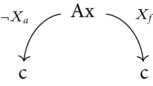
3.3 Relation to MLL model
In Murfet and Troiani (Reference Murfet and Troiani2022), we attributed to an Axiom-link

the equation
 \begin{equation} X_1 - X_2 \in \mathbb{k}[X_1,X_2]. \end{equation}
In this paper, we have attributed to (143) the composite of closed immersions
 \begin{equation} \Delta \longrightarrow \mathbb{P}^1 \times \mathbb{P}^1 \longrightarrow \mathbb{P}^3 \end{equation}
where
 $\Delta \longrightarrow \mathbb{P}^1 \times \mathbb{P}^1$
is the diagonal and
$\Delta \longrightarrow \mathbb{P}^1 \times \mathbb{P}^1$
is the diagonal and
 $\mathbb{P}^1 \times \mathbb{P}^1 \longrightarrow \mathbb{P}^3$
is the Segre embedding. We remark that
$\mathbb{P}^1 \times \mathbb{P}^1 \longrightarrow \mathbb{P}^3$
is the Segre embedding. We remark that
 \begin{equation} \operatorname {Proj}\big ((\mathbb{k}[X_1',X_1] \times _{\mathbb{k}} \mathbb{k}[X_2', X_2])/(X_1X_2' - X_1'X_2)\big ) \cong \Delta \end{equation}
where we have made use of the Cartesian product
 $\times _{\mathbb{k}}$
, see Definition 3.0.7. Thus, algebraically, we can think of the present model as attributing to (143) the equation
$\times _{\mathbb{k}}$
, see Definition 3.0.7. Thus, algebraically, we can think of the present model as attributing to (143) the equation
 \begin{equation} X_1X_2' - X_1'X_2 \in \mathbb{k}[X_1',X_1] \times _{\mathbb{k}} \mathbb{k}[X_2', X_2]. \end{equation}
We saw in Section 3.2.1 that we can recover (144) from (147) by dividing by the primed variables. That is, the composition of isomorphisms
 \begin{equation} (\mathbb{k}[X_1',X_1] \times _{\mathbb{k}}\mathbb{k}[X_2', X_2] )_{(X_1'X_2')} \longrightarrow \mathbb{k}[X_1/X_1', X_2/X_2'] \longrightarrow \mathbb{k}[X_1, X_2] \end{equation}
determined by the rules
 \begin{equation} \frac {X_1X_2'}{X_1'X_2'} \longmapsto X_1/X_1' \longmapsto X_1,\quad \frac {X_1'X_2}{X_1'X_2'} \longmapsto X_2/X_2' \longmapsto X_2 \end{equation}
maps (147) to (144). Lemma 3.3.3 generalises this observation to all of MLL and makes precise the claim that Theorem3.1.3 generalises (Murfet and Troiani Reference Murfet and Troiani2022, Proposition 4.6), we make use of the notation there.
Let
 $A$
be a linear formula with
$A$
be a linear formula with
 $n$
unoriented atoms
$n$
unoriented atoms
 $\{X_1, \ldots , X_n\}$
so that
$\{X_1, \ldots , X_n\}$
so that
 $P_A = \mathbb{k}[X_1, \ldots , X_n]$
, where
$P_A = \mathbb{k}[X_1, \ldots , X_n]$
, where
 $P_A$
is the polynomial ring associated to
$P_A$
is the polynomial ring associated to
 $A$
of Murfet and Troiani (Reference Murfet and Troiani2022, Definition 3.14). This is the coordinate ring of the scheme
$A$
of Murfet and Troiani (Reference Murfet and Troiani2022, Definition 3.14). This is the coordinate ring of the scheme
 $\mathbb{A}_{\mathbb{k}}^n$
which is an open subset of the product
$\mathbb{A}_{\mathbb{k}}^n$
which is an open subset of the product
 $(\mathbb{P}_{\mathbb{k}}^1)^n$
. Let
$(\mathbb{P}_{\mathbb{k}}^1)^n$
. Let
 $\pi$
be a proof in MLL.
$\pi$
be a proof in MLL.
Definition 3.3.1.
For all
 $n\gt 0$
, let
$n\gt 0$
, let
 $S_n$
denote the
$S_n$
denote the
 $\mathbb{k}$
-algebra
$\mathbb{k}$
-algebra
 \begin{equation} S_n = \mathbb{k}[x_1,x_1'] \times _{\mathbb{k}} \ldots \times _{\mathbb{k}}\mathbb{k}[x_n,x_n']. \end{equation}
For each
 $n\gt 0$
, fix an isomorphism
$n\gt 0$
, fix an isomorphism
 \begin{equation} \Phi _n: \operatorname {Proj}S_n \longrightarrow (\mathbb{P}_{\mathbb{k}}^1)^n. \end{equation}
We also fix isomorphisms
 \begin{equation} \Psi _n: \operatorname {Spec}(\mathbb{k}[x_1,\ldots , x_n]) \longrightarrow \operatorname {Spec}\Big (\big (S_n)_{(x_1'\ldots x_n')}\Big ). \end{equation}
We have a composition
 \begin{equation} \mathbb{A}_{\mathbb{k}}^n = \operatorname {Spec}(\mathbb{k}[x_1,\ldots , x_n]) \stackrel {\psi _n}{\longrightarrow } \operatorname {Spec}\Big (\big (S_n)_{(x_1'\ldots x_n')}\Big ) \stackrel {\Phi _n}{\longrightarrow } (\mathbb{P}_{\mathbb{k}}^1)^n \longrightarrow \mathbb{S}(A) \end{equation}
where the final map is the Segre embedding. If
 $\pi$
is a proof in MLL, we take the product of these over all formulas
$\pi$
is a proof in MLL, we take the product of these over all formulas
 $A_e$
labelling edges
$A_e$
labelling edges
 $e$
of
$e$
of
 $\pi$
to obtain an inclusion
$\pi$
to obtain an inclusion
 \begin{equation} \iota _{\pi }:\operatorname {Spec}P_\pi \cong \prod _{e \in \mathcal{E}_\pi }\mathbb{A}_{\mathbb{k}}^{|U_{A_e}|} \longrightarrow \mathbb{S}(\pi ) \end{equation}
where
 $P_\pi$
is the polynomial ring associated to
$P_\pi$
is the polynomial ring associated to
 $\pi$
as defined in Murfet and Troiani (Reference Murfet and Troiani2022, Definition 3.14), and
$\pi$
as defined in Murfet and Troiani (Reference Murfet and Troiani2022, Definition 3.14), and
 $U_{A_e}$
denotes the set of unoriented atoms of
$U_{A_e}$
denotes the set of unoriented atoms of
 $A_e$
as defined in Murfet and Troiani (Reference Murfet and Troiani2022, Definition 3.7).
$A_e$
as defined in Murfet and Troiani (Reference Murfet and Troiani2022, Definition 3.7).
Definition 3.3.2.
Given a reduction
 $\gamma : \pi \longrightarrow \pi '$
of proofs
$\gamma : \pi \longrightarrow \pi '$
of proofs
 $\pi , \pi '$
in MLL, let
$\pi , \pi '$
in MLL, let
 $S^\bullet , T^\bullet$
denote the
$S^\bullet , T^\bullet$
denote the
 $\mathbb{k}$
-algebra homomorphisms defined as
$\mathbb{k}$
-algebra homomorphisms defined as
 $S,T$
in Murfet and Troiani (Reference Murfet and Troiani2022, Proposition 4.6).
$S,T$
in Murfet and Troiani (Reference Murfet and Troiani2022, Proposition 4.6).
Lemma 3.3.3.
For any reduction
 $\gamma : \pi \longrightarrow \pi '$
where
$\gamma : \pi \longrightarrow \pi '$
where
 $\pi , \pi '$
are proofs in MLL, there exists the following commuting diagrams:
$\pi , \pi '$
are proofs in MLL, there exists the following commuting diagrams:
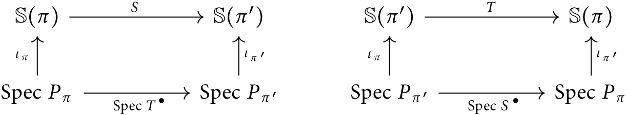
Proof.
In this case, the maps
 $S, T$
are either projections or diagonal morphisms. Thus, for the statement to hold, one must check that
$S, T$
are either projections or diagonal morphisms. Thus, for the statement to hold, one must check that
 $\operatorname {Spec}T^\bullet , \operatorname {Spec}S^\bullet$
are the appropriate restrictions of these. This is done by inspection along with (a generalisation of) the fact that the diagonal morphism
$\operatorname {Spec}T^\bullet , \operatorname {Spec}S^\bullet$
are the appropriate restrictions of these. This is done by inspection along with (a generalisation of) the fact that the diagonal morphism
 $\Delta : \mathbb{A}_{\mathbb{k}}^1 \longrightarrow \mathbb{A}_{\mathbb{k}}^2$
is
$\Delta : \mathbb{A}_{\mathbb{k}}^1 \longrightarrow \mathbb{A}_{\mathbb{k}}^2$
is
 $\operatorname {Spec}(f)$
where
$\operatorname {Spec}(f)$
where
 $f: \mathbb{k}[x_1, x_2] \longrightarrow \mathbb{k}[x]$
is the
$f: \mathbb{k}[x_1, x_2] \longrightarrow \mathbb{k}[x]$
is the
 $\mathbb{k}$
-algebra homomorphism mapping
$\mathbb{k}$
-algebra homomorphism mapping
 $x_1 \longmapsto x, x_2 \longmapsto x$
, along with (a generalisation of) the fact that the projection (for
$x_1 \longmapsto x, x_2 \longmapsto x$
, along with (a generalisation of) the fact that the projection (for
 $i = 1,2$
)
$i = 1,2$
)
 $\operatorname {Projection}_i: \mathbb{A}_{\mathbb{k}}^2 \longrightarrow \mathbb{A}_{\mathbb{k}}^1$
is
$\operatorname {Projection}_i: \mathbb{A}_{\mathbb{k}}^2 \longrightarrow \mathbb{A}_{\mathbb{k}}^1$
is
 $\operatorname {Spec}(g_i)$
where
$\operatorname {Spec}(g_i)$
where
 $g_i: \mathbb{k}[x] \longrightarrow \mathbb{k}[x_1, x_2]$
is the
$g_i: \mathbb{k}[x] \longrightarrow \mathbb{k}[x_1, x_2]$
is the
 $\mathbb{k}$
-algebra homomorphism mapping
$\mathbb{k}$
-algebra homomorphism mapping
 $x \longmapsto x_i$
.
$x \longmapsto x_i$
.
4. Future paths
Extending the model to all of MELL. The immediate obstruction to extending our model to all of MELL is Lemma 3.0.10, which only considers shallow proofs. We postulate that this lemma does indeed generalise. To check this, one must check that the local freeness condition is satisfied by the immersion (37). However, it is not precisely this lemma which would be generalised. A difficulty in working with our model is the fact that we have defined the Hilbert scheme
 $H_T$
to parameterise graded
$H_T$
to parameterise graded
 $\mathbb{k}$
-modules
$\mathbb{k}$
-modules
 $T$
. In fact, a more general Hilbert scheme exists, which is parameterised by projective schemes instead. Similarly to
$T$
. In fact, a more general Hilbert scheme exists, which is parameterised by projective schemes instead. Similarly to
 $H_T$
, the more general Hilbert scheme represents a functor. The reference for this is Grothendieck (Reference Grothendieck1961).
$H_T$
, the more general Hilbert scheme represents a functor. The reference for this is Grothendieck (Reference Grothendieck1961).
Definition 4.0.1.
Suppose
 $S$
is a locally Noetherian scheme and
$S$
is a locally Noetherian scheme and
 $X \longrightarrow S$
is a projective scheme over
$X \longrightarrow S$
is a projective scheme over
 $S$
. The
Hilbert functor
from the category
$S$
. The
Hilbert functor
from the category
 $\underline {\operatorname {Sch}}_{S}$
whose objects are locally Noetherian schemes over
$\underline {\operatorname {Sch}}_{S}$
whose objects are locally Noetherian schemes over
 $S$
to the category
$S$
to the category
 $\underline {\operatorname {Set}}$
of sets is given by:
$\underline {\operatorname {Set}}$
of sets is given by:
 \begin{align*} \operatorname {Hilb}_{X/S}: \underline {\operatorname {Sch}}_{S} &\longrightarrow \underline {\operatorname {Set}}\\ T &\longmapsto \{\text{Closed subschemes }Z \longrightarrow X \times _S T \mid \\ &\quad \quad Z \text{ is flat over }T\}. \end{align*}
Theorem 4.0.2.
There exists a scheme
 $\operatorname {Hilb}_{X/S}$
representing this functor.
$\operatorname {Hilb}_{X/S}$
representing this functor.
This is a more interesting functor for us because it yields a simple way of thinking about Pax-links: they give rise to the product of locally projective schemes
 $X_1 \times \cdots \times X_n$
over which the closed subscheme corresponding to the interior of the box must be flat. In particular, this will avoid all necessity of localisation inside Definition 3.0.4, which we believe would lead to a more natural model.
$X_1 \times \cdots \times X_n$
over which the closed subscheme corresponding to the interior of the box must be flat. In particular, this will avoid all necessity of localisation inside Definition 3.0.4, which we believe would lead to a more natural model.
Thus, our future work proposal is as follows: first, we extend the model for shallow proofs to one where the Hilbert scheme
 $H_T$
is replaced by the more general Hilbert scheme
$H_T$
is replaced by the more general Hilbert scheme
 $\operatorname {Hilb}_{X/S}$
above. Then, we would aim to extend the resulting model to all of MELL. Of course, one could also dream of going even further than MELL; additives, differential linear logic, etc.
$\operatorname {Hilb}_{X/S}$
above. Then, we would aim to extend the resulting model to all of MELL. Of course, one could also dream of going even further than MELL; additives, differential linear logic, etc.
Relating this model to the MLL models given in Chapter (Troiani Reference Troiani2024, Chapter IV). We presented three models of MLL in total in Troiani (Reference Troiani2024). One gives proofs as linear equations, which have been extended to shallow proofs inside this paper (as well as in Troiani (Reference Troiani2024, Chapter III). The other two give proofs as matrix factorisations and proofs as quantum error correction codes, respectively. Section (Troiani Reference Troiani2024, Section 4.2.5) relates the algebraic model to the quantum error correction code model via the matrix factorisation one, and so it would be interesting to see how the Hilbert scheme plays a role in these other models. For instance, the Hilbert scheme plays the role of a moduli space, in that it parameterises flat families of closed subschemes. It would be interesting to consider the moduli space of matrix factorisations as a possible model in the sense of Fiore et al. (Reference Fiore, Gambino and Hyland2024) of the exponential in linear logic.
Classifying the Hilbert functions which arise from proofs. Our model considers the set
 $\mathcal{H}$
of all Hilbert functions throughout. Surely not all Hilbert functions arise from proofs. It would be interesting to find the subset
$\mathcal{H}$
of all Hilbert functions throughout. Surely not all Hilbert functions arise from proofs. It would be interesting to find the subset
 $\mathcal{H}' \subseteq \mathcal{H}$
so that
$\mathcal{H}' \subseteq \mathcal{H}$
so that
 $h \in \mathcal{H}'$
if and only if there exists a proof
$h \in \mathcal{H}'$
if and only if there exists a proof
 $\pi$
such that the closed subscheme
$\pi$
such that the closed subscheme
 $\mathbb{X}(\pi ) \longrightarrow \mathbb{S}(\pi )$
has Hilbert function
$\mathbb{X}(\pi ) \longrightarrow \mathbb{S}(\pi )$
has Hilbert function
 $h$
.
$h$
.
It has been noted in Troiani (Reference Troiani2024, Remark 2.12) that there is more to the Geometry of Interaction programme than just modelling cut-elimination with a non-trivial effective procedure. One could also ask for a correctness criterion, such as the long trip condition given in the Sequentialisation Theorem (due to Girard (1987)), to be present in our model as well. It is possible that the classification of the Hilbert functions which arise from proofs has relevance to this line of research.
Elimination theory. The algebraic model given in Murfet and Troiani (Reference Murfet and Troiani2022) not only gives an interpretation of proofs in MLL but also relates the cut-elimination process to the Buchberger algorithm. As mentioned in Remark 3.2.2, it seems possible that this relationship extends to MELL, at least to shallow proofs. There are many connections to the construction of the (multigraded) Hilbert scheme of Haiman and Sturmfels (Reference Haiman and Sturmfels2002) and syzygies, monomial ideals, Gröbner bases, etc. These connections should be fully developed.
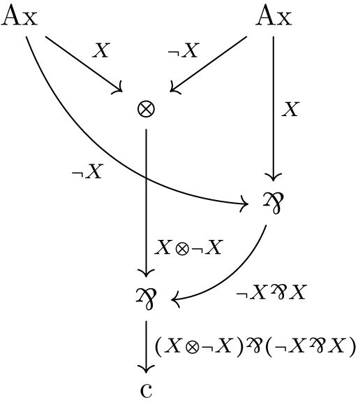

 Open access