


1. Introduction
The study of product sets $A \cdot B \;:\!=\; \{ab \;:\; a \in A, b \in B\}$
of two sets of natural numbers A and B has long been of interest in mathematics. For finite sets, the classic multiplication table problem, posed by Erdös [
Reference Erdös4, Reference Erdös5
], seeks bounds on the cardinality of the
$A \cdot B \;:\!=\; \{ab \;:\; a \in A, b \in B\}$
of two sets of natural numbers A and B has long been of interest in mathematics. For finite sets, the classic multiplication table problem, posed by Erdös [
Reference Erdös4, Reference Erdös5
], seeks bounds on the cardinality of the $n\times n$
multiplication table. The correct order of magnitude was established by Ford [
Reference Ford6
], building on earlier work by Tenenbaum [
Reference Tenenbaum18
] (cf. [
Reference Hall and Tenenbaum10
]). The existence of an asymptotic formula for this problem remains open. A multidimensional variation was later studied by Koukoulopoulos [
Reference Koukoulopoulos13
]. For more general finite sets, the cardinality problem has been investigated by Cilleruelo, Ramana, and Ramaré [
Reference Cilleruelo, Ramana and Ramaré3
], as well as by Mastrostefano [
Reference Mastrostefano15
] and Sanna [
Reference Sanna16
].
$n\times n$
multiplication table. The correct order of magnitude was established by Ford [
Reference Ford6
], building on earlier work by Tenenbaum [
Reference Tenenbaum18
] (cf. [
Reference Hall and Tenenbaum10
]). The existence of an asymptotic formula for this problem remains open. A multidimensional variation was later studied by Koukoulopoulos [
Reference Koukoulopoulos13
]. For more general finite sets, the cardinality problem has been investigated by Cilleruelo, Ramana, and Ramaré [
Reference Cilleruelo, Ramana and Ramaré3
], as well as by Mastrostefano [
Reference Mastrostefano15
] and Sanna [
Reference Sanna16
].
The analogous problem for infinite sets of natural numbers was considered by Hegyvári, Hennecart, and Pach [
Reference Hegyvári, Hennecart and Pach11
]. In this context, the role of cardinality is played by the natural density $d(A)\;:\!=\; \lim_{x\rightarrow \infty } ({\# (A \cap [1,x])}/{x})$
of a set A, if the limit exists. Hegyvári, Hennecart and Pach asked whether, given two sets A, B with density 1, the product set
$d(A)\;:\!=\; \lim_{x\rightarrow \infty } ({\# (A \cap [1,x])}/{x})$
of a set A, if the limit exists. Hegyvári, Hennecart and Pach asked whether, given two sets A, B with density 1, the product set $A \cdot B$
also has density 1.
$A \cdot B$
also has density 1.
In [ Reference Bettin, Koukoulopoulos and Sanna2 ], Bettin, Koukoulopoulos and Sanna answered this question in the affirmative. In other words, defining
 \begin{align}{\mathrm{R}}_x(A) \;:\!=\; 1 - \frac{\# (A \cap [1,x])}{x}\end{align}
for any $A \subseteq \mathbb{N}$
and
$A \subseteq \mathbb{N}$
and $x \geq 1$
, they proved that if
$x \geq 1$
, they proved that if ${\mathrm{R}}_x(A),{\mathrm{R}}_x(B) \to 0$
as
${\mathrm{R}}_x(A),{\mathrm{R}}_x(B) \to 0$
as $x \to \infty$
, then also
$x \to \infty$
, then also ${\mathrm{R}}_x(A \cdot B) \to 0$
. In the same paper, it was also remarked that one could obtain an explicit rate of convergence for
${\mathrm{R}}_x(A \cdot B) \to 0$
. In the same paper, it was also remarked that one could obtain an explicit rate of convergence for ${\mathrm{R}}_x(A \cdot A)$
in terms of the rate of
${\mathrm{R}}_x(A \cdot A)$
in terms of the rate of ${\mathrm{R}}_x(A)$
. More specifically, their proof (cf. [
Reference Bettin, Koukoulopoulos and Sanna2
, remark, p.1411]) gives that if
${\mathrm{R}}_x(A)$
. More specifically, their proof (cf. [
Reference Bettin, Koukoulopoulos and Sanna2
, remark, p.1411]) gives that if
 $${\mathrm{R}}_x(A)\ll (\!\log x)^{-a} \quad \text{ for some } a\in(0,1),$$
then
 \begin{align*} {\mathrm{R}}_x(A\cdot A)\ll (\!\log x)^{-\frac{a^2}{1+a}+o(1)}.\end{align*}
Equivalently, letting
 \begin{align*}\psi(a)&\;:\!=\;\sup \Big\{b\in{\mathbb R}_{\gt 0}\ \Big|\ {\mathrm{R}}_{x}(A\cdot A)\ll (\!\log x)^{-b} \ \forall A{\subseteq}{\mathbb N}\text{ s.t. }{\mathrm{R}}_x(A)\ll(\!\log x)^{-a}\Big\}\\&\hphantom{:}=\inf_{A{\subseteq} \mathbb N \atop {\mathrm{R}}_x(A)\ll (\!\log x)^{-a}\hspace{-1.em}}\big\{b\in{\mathbb R}_{\gt 0}\ \big|\ {\mathrm{R}}_x(A\cdot A)=\Omega( (\!\log x)^{-b} )\big\}\end{align*}
for $a\gt 0$
, the result of [
Reference Bettin, Koukoulopoulos and Sanna2
] establishes that
$a\gt 0$
, the result of [
Reference Bettin, Koukoulopoulos and Sanna2
] establishes that $\psi(a) \geq a^2/(1+a)$
for
$\psi(a) \geq a^2/(1+a)$
for $a\in(0,1)$
. In this note, we aim to make progress on determining the function
$a\in(0,1)$
. In this note, we aim to make progress on determining the function $\psi(a)$
by providing an upper bound. It is easy to see that
$\psi(a)$
by providing an upper bound. It is easy to see that $\psi(a)\leq a$
for all
$\psi(a)\leq a$
for all $a\in(0,1)$
. Indeed, let us denote by P a subset of the primes with relative asymptotic density
$a\in(0,1)$
. Indeed, let us denote by P a subset of the primes with relative asymptotic density $a\in(0,1)$
, i.e.
$a\in(0,1)$
, i.e. ${\#}(P\cap[1,x])\sim ax/\log x$
. Then, letting
${\#}(P\cap[1,x])\sim ax/\log x$
. Then, letting
 $$A_P\;:\!=\;\{n\in{\mathbb N}\mid \exists p\in P\text{ s.t. $p|n$}\}\cup\{1\}$$
we have $A_P\cdot A_P=A_P$
and, by the Fundamental Lemma of Sieve Theory [
Reference Koukoulopoulos12
, theorem 18·11],
$A_P\cdot A_P=A_P$
and, by the Fundamental Lemma of Sieve Theory [
Reference Koukoulopoulos12
, theorem 18·11],
 $${\mathrm{R}}_x(A_P)={\mathrm{R}}_x(A_P\cdot A_P)=\frac1x\#\{n\in[2,x]\mid (p,n)=1\, \forall p\in P\}=(\!\log x)^{-a+o(1)}.$$
We improve upon this “trivial” bound for sufficiently small values of a. More specifically, we show the following.
Theorem 1·1. For $a\in(0,1/4)$
,
$a\in(0,1/4)$
, $B\in [0,\phi^{-1}(4a)]$
, let
$B\in [0,\phi^{-1}(4a)]$
, let
 \begin{align}W(a,B)\;:\!=\;a\frac{\phi(2B)}{\phi(B)}+\frac{(\phi(B)-\sqrt{\phi(B)^2-4a \phi(B)})^2}{4\phi(B)},\end{align}
where $\phi:[0,1]\to[0,1]$
is defined by
$\phi:[0,1]\to[0,1]$
is defined by
 \begin{align}\phi(x)\;:\!=\;\begin{cases}x\log x-x+1, & x\in(0,1),\\1 &x=0.\end{cases}\end{align}
Then, defining
 \begin{align}K(a)&\;:\!=\; \min_{\substack{ B\in [0,\phi^{-1}(4a)]}}W(a,B),\qquad a\in(0,1/4),\end{align}
we have
 \begin{align}\psi(a)\leq K(a).\end{align}
Moreover, one has
 \begin{align}&K(a)\lt a && \text{ for } a\in(0,0.11717],\end{align}
 \begin{align}&K(a)\le \frac{2a^2}{1-\log 2}+o(a^2) && \text{ as }a\to0^+.\end{align}
We conclude the Introduction by noting that, together with the bound of [
Reference Bettin, Koukoulopoulos and Sanna2
], (1·7) implies that $\psi(a)$
decays quadratically as
$\psi(a)$
decays quadratically as $a\to0^+$
. More precisely,
$a\to0^+$
. More precisely,
 $$1\leq\liminf_{a\to0^+}\frac{\psi(a)}{a^2}\leq \limsup_{a\to0^+}\frac{\psi(a)}{a^2}\leq \frac{2}{1-\log2}=6.51778\ldots.$$
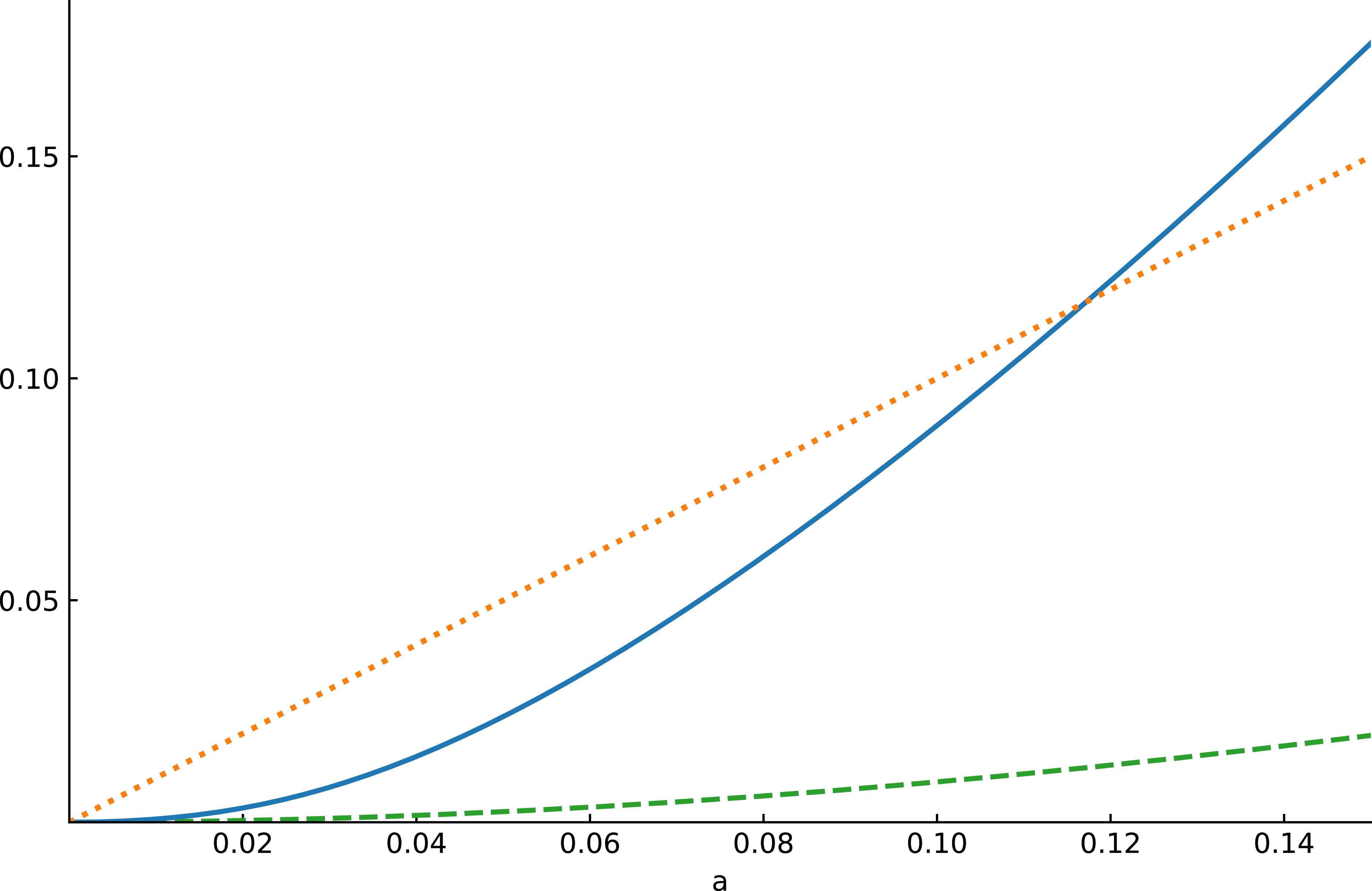
A visual representation of these bounds is given in Figure 1.
The functions ${a^2}/({1+a})$
(dashed), K(a) (continuous) and a (dotted) for
${a^2}/({1+a})$
(dashed), K(a) (continuous) and a (dotted) for $0\leq a\leq0.15$
. The function
$0\leq a\leq0.15$
. The function $\psi$
lies between the dashed curve and the minimum between the continuous and the dotted curves.
$\psi$
lies between the dashed curve and the minimum between the continuous and the dotted curves.

1·1. Sketch of the argument
The main idea used in [ Reference Bettin, Koukoulopoulos and Sanna2 ] is as follows: any integer n can be factorised as
 \[n = n_{\text{smooth}} \cdot n_{\text{rough}},\]
where $n_{\text{smooth}}$
and
$n_{\text{smooth}}$
and $n_{\text{rough}}$
are the products of its “small” and “large” prime factors, respectively, with respect to a suitably chosen (small) cutoff. If
$n_{\text{rough}}$
are the products of its “small” and “large” prime factors, respectively, with respect to a suitably chosen (small) cutoff. If $n \notin A \cdot A$
, then at least one of these factors must be missing from A, meaning either
$n \notin A \cdot A$
, then at least one of these factors must be missing from A, meaning either $n_{\text{smooth}} \notin A$
or
$n_{\text{smooth}} \notin A$
or $n_{\text{rough}} \notin A$
. If the product set
$n_{\text{rough}} \notin A$
. If the product set $A \cdot A$
does not have density 1, then A must lack its expected proportion of either smooth or rough numbers. Consequently, A itself cannot have density 1.
$A \cdot A$
does not have density 1, then A must lack its expected proportion of either smooth or rough numbers. Consequently, A itself cannot have density 1.
In the argument above, for any $n\notin A\cdot A$
one infers information about A from a single factorisation of n, where n is written as a product of two integers. These integers, in addition to not both belonging to A, also satisfy the extra condition of being respectively small and smooth, and large and rough. To construct a set A such that
$n\notin A\cdot A$
one infers information about A from a single factorisation of n, where n is written as a product of two integers. These integers, in addition to not both belonging to A, also satisfy the extra condition of being respectively small and smooth, and large and rough. To construct a set A such that $ \mathbb{N} \setminus (A \cdot A) $
is large, we aim to define A in a way that naturally forces a typical integer m to have all its factorisations in
$ \mathbb{N} \setminus (A \cdot A) $
is large, we aim to define A in a way that naturally forces a typical integer m to have all its factorisations in $ A \cdot A $
constrained by this extra condition.
$ A \cdot A $
constrained by this extra condition.
To achieve this, we define A as the set of integers that do not have “too few” large prime divisors, i.e., we consider
 \[A = \big\{ m \;:\; \Omega^*(m) \gt B {\mathrm{M}}(m) \big\},\]
where
 \[\Omega^*(m) = \sum_{\substack{p^{\nu_p} {\mid\!\mid} m \\ \exp(\delta \log\log m) \lt p \leq m}} \nu_p,\qquad {\mathrm{M}}(m) = (1-\delta)\log\log m.\]
Notice that ${\mathrm{M}}(m)$
is the asymptotic value of
${\mathrm{M}}(m)$
is the asymptotic value of $\Omega^*(m)$
for a typical integer
$\Omega^*(m)$
for a typical integer $m\in{\mathbb N}$
. Here
$m\in{\mathbb N}$
. Here $\delta, B \in (0,1)$
are arbitrary parameters satisfying
$\delta, B \in (0,1)$
are arbitrary parameters satisfying $(1-\delta)\phi(B)=a$
, so that
$(1-\delta)\phi(B)=a$
, so that ${\mathrm{R}}_x(A) = (\!\log x)^{-(1-\delta)\phi(B)+o(1)}=(\!\log x)^{-a+o(1)}.$
For any factorisation $m = n_1 n_2$
with
$m = n_1 n_2$
with $n_1, n_2 \in A$
and
$n_1, n_2 \in A$
and $n_1 \leq n_2$
, we have two possibilities:
$n_1 \leq n_2$
, we have two possibilities:
-
(1) if $n_1$
and
$n_2$
are of comparable size, then
$ \Omega^*(m) \gtrsim B ( {\mathrm{M}}(n_1) + {\mathrm{M}}(n_2) ) \approx 2B {\mathrm{M}}(m)$
;
$n_1$
and
$n_2$
are of comparable size, then
$ \Omega^*(m) \gtrsim B ( {\mathrm{M}}(n_1) + {\mathrm{M}}(n_2) ) \approx 2B {\mathrm{M}}(m)$
; -
(2) if
$n_1$
is much smaller than
$n_2$
, then m has at least
$B {\mathrm{M}}(n_1)$
prime divisors smaller than
$n_1$
, and thus m does not have too few prime divisors of such (small) size.





Letting $I_1$
and
$I_1$
and $I_2$
denote the sets of integers satisfying conditions (1) and (2) respectively, we thus have
$I_2$
denote the sets of integers satisfying conditions (1) and (2) respectively, we thus have $A\cdot A\subseteq I_1\cup I_2$
. The conditions (1) and (2) are roughly independent, and therefore
$A\cdot A\subseteq I_1\cup I_2$
. The conditions (1) and (2) are roughly independent, and therefore ${\mathrm{R}}_x(A\cdot A)\gtrsim {\mathrm{R}}_x(I_1)\cdot {\mathrm{R}}_x(I_2)$
. We then optimise the choice of
${\mathrm{R}}_x(A\cdot A)\gtrsim {\mathrm{R}}_x(I_1)\cdot {\mathrm{R}}_x(I_2)$
. We then optimise the choice of $\delta$
and B, subject to the constraint
$\delta$
and B, subject to the constraint $(1-\delta)\phi(B)=a$
, to maximise the product
$(1-\delta)\phi(B)=a$
, to maximise the product ${\mathrm{R}}_x(I_1)\cdot {\mathrm{R}}_x(I_2)$
. This yields (1·4), where the factors
${\mathrm{R}}_x(I_1)\cdot {\mathrm{R}}_x(I_2)$
. This yields (1·4), where the factors ${\mathrm{R}}_x(I_1)$
and
${\mathrm{R}}_x(I_1)$
and ${\mathrm{R}}_x(I_2)$
correspond to the two summands in (1·2).
${\mathrm{R}}_x(I_2)$
correspond to the two summands in (1·2).
Both (1) and (2) impose conditions on m that are satisfied less frequently than the condition $\Omega^*(m) \gt B {\mathrm{M}}(m)$
in the definition of A. Thus,
$\Omega^*(m) \gt B {\mathrm{M}}(m)$
in the definition of A. Thus, ${\mathrm{R}}_x(I_1),{\mathrm{R}}_x(I_2)\gtrsim {\mathrm{R}}_x(A) (\!\log x)^{\kappa_a}$
for some
${\mathrm{R}}_x(I_1),{\mathrm{R}}_x(I_2)\gtrsim {\mathrm{R}}_x(A) (\!\log x)^{\kappa_a}$
for some $\kappa_a\gt 0$
. While it is not a priori guaranteed that a similar bound holds for the product
$\kappa_a\gt 0$
. While it is not a priori guaranteed that a similar bound holds for the product ${\mathrm{R}}_x(I_1)\cdot{\mathrm{R}}_x(I_2)$
, this indeed holds if a is small enough, provided the parameters are chosen suitably. Indeed, if we take for example
${\mathrm{R}}_x(I_1)\cdot{\mathrm{R}}_x(I_2)$
, this indeed holds if a is small enough, provided the parameters are chosen suitably. Indeed, if we take for example $B=1/2$
one has
$B=1/2$
one has ${\mathrm{R}}_x(I_1)\asymp1$
and
${\mathrm{R}}_x(I_1)\asymp1$
and ${\mathrm{R}}_x(I_2)\gg (\!\log x)^{-O(a^2)}$
, whereas by definition
${\mathrm{R}}_x(I_2)\gg (\!\log x)^{-O(a^2)}$
, whereas by definition ${\mathrm{R}}_x(A)=(\!\log x)^{-a+o(1)}$
. A more careful examination shows that any
${\mathrm{R}}_x(A)=(\!\log x)^{-a+o(1)}$
. A more careful examination shows that any $a\leq 0.11717$
is admissible, giving (1·6).
$a\leq 0.11717$
is admissible, giving (1·6).
When making this argument rigorous, we need to make an additional refinement. Specifically, we modify $\Omega^*(m)$
to “discretise” the interval
$\Omega^*(m)$
to “discretise” the interval $(\exp(\delta \log\log m), m]$
in its definition. See (3·1) for the precise definition of the set A. This adjustment is needed when handling all the possible range constraints in case (2).
$(\exp(\delta \log\log m), m]$
in its definition. See (3·1) for the precise definition of the set A. This adjustment is needed when handling all the possible range constraints in case (2).
1·2. Notation
Throughout the paper, we will employ the following standard notation. Given integers a, b, and m, we write $a| b$
if a divides b, and
$a| b$
if a divides b, and $a^m \| b$
if
$a^m \| b$
if $a^m$
divides b exactly, i.e.
$a^m$
divides b exactly, i.e. $a^m|b$
and
$a^m|b$
and $a^{m+1}\nmid b$
. We also employ Landau’s notation
$a^{m+1}\nmid b$
. We also employ Landau’s notation $f= O(g)$
and Vinogradov’s notation
$f= O(g)$
and Vinogradov’s notation $f \ll g$
, both meaning that
$f \ll g$
, both meaning that $|f|\leq C|g|$
for some constant
$|f|\leq C|g|$
for some constant $C \gt 0$
. If the constant C depends on some parameter y, we write
$C \gt 0$
. If the constant C depends on some parameter y, we write $f=O_y(g)$
or
$f=O_y(g)$
or $f\ll_y g$
. The notation
$f\ll_y g$
. The notation $f= o(g)$
as
$f= o(g)$
as $x\to a$
means that
$x\to a$
means that $\lim_{x\to a} f(x)/g(x) = 0$
. Finally, we write
$\lim_{x\to a} f(x)/g(x) = 0$
. Finally, we write $f=\Omega_y(|g|)$
as
$f=\Omega_y(|g|)$
as $x\to a$
if there exist a constant
$x\to a$
if there exist a constant $c=c(y)\gt 0$
and a sequence
$c=c(y)\gt 0$
and a sequence $x_n\to a$
such that
$x_n\to a$
such that $|f(x_n)|\geq c|g(x_n)|$
.
$|f(x_n)|\geq c|g(x_n)|$
.
2. Lemmata
For any set of primes S, we denote
 $${\mathrm{S}}(x)\;:\!=\; \sum_{\substack{p\leq x \\ p\in S}}\frac{1}{p},\qquad \Omega(n;\;S) \;:\!=\; \sum_{\substack{p^{\nu_p} {\mid\!\mid} n \\ p\in S}} \nu_p. $$
All the preliminary results stated in this section are manifestations of the Poissonian nature of the arithmetic function $\Omega(n;\;S)$
. The first one is a standard upper bound for the probability that a random integer n has a limited number of prime divisors in an interval.
$\Omega(n;\;S)$
. The first one is a standard upper bound for the probability that a random integer n has a limited number of prime divisors in an interval.
Lemma 2·1. Let $\phi$
be as in (1·3). Then, uniformly for
$\phi$
be as in (1·3). Then, uniformly for $e\lt U\lt V\leq \log\log x$
and
$e\lt U\lt V\leq \log\log x$
and $B\in[0,1)$
, we have
$B\in[0,1)$
, we have
 $$\frac{1}{x}\sum_{\substack{n\leq x \atop \Omega(n;\;(U,V])\leq B\log\frac{\log V}{\log U}}}1 \ll \bigg(\frac{\log V}{\log U}\bigg)^{-\phi(B)} . $$
Proof. Halász [
Reference Halász9
] proved sharp bounds for integers $n\leq x$
with
$n\leq x$
with $\Omega(n;\;(U,V])=k$
. To obtain the claimed result it suffices to sum over
$\Omega(n;\;(U,V])=k$
. To obtain the claimed result it suffices to sum over $k\leq B\log({\log V}/{\log U})$
.
$k\leq B\log({\log V}/{\log U})$
.
Building on works of Halász [
Reference Halász8, Reference Halász9
], Sárközy [
Reference Sárközy17
] (see also [
Reference Balazard1
, Theorem A and subsequent paragraphs on page 391]) obtained a lower bound for the number of integers with $\Omega(n;\;S)=k$
. We need a version of this (with
$\Omega(n;\;S)=k$
. We need a version of this (with $\Omega(n;\;S)\leq k$
) where there are multiple conditions on the number of prime divisors in disjoint sets. This is obtained in Tenenbaum [
Reference Tenenbaum19
], but only when k is not too small. See also [
Reference Ford7, Reference Mangerel14, Reference Tudesq20
] for some related results. We provide a short proof of the precise result that we need by making simple modifications to [
Reference Halász9
], being very brief in the steps that are essentially identical to Halász’ work.
$\Omega(n;\;S)\leq k$
) where there are multiple conditions on the number of prime divisors in disjoint sets. This is obtained in Tenenbaum [
Reference Tenenbaum19
], but only when k is not too small. See also [
Reference Ford7, Reference Mangerel14, Reference Tudesq20
] for some related results. We provide a short proof of the precise result that we need by making simple modifications to [
Reference Halász9
], being very brief in the steps that are essentially identical to Halász’ work.
Lemma 2·2. Let $m\in\mathbb N$
,
$m\in\mathbb N$
, $\underline k = (k_1,\ldots,k_m)\in\mathbb N^m$
,
$\underline k = (k_1,\ldots,k_m)\in\mathbb N^m$
, $\varepsilon\gt 0$
and
$\varepsilon\gt 0$
and $x\geq1$
. Let
$x\geq1$
. Let $S_1,\ldots,S_m$
disjoint sets of primes. Then, for
$S_1,\ldots,S_m$
disjoint sets of primes. Then, for $A_\varepsilon$
large enough we have
$A_\varepsilon$
large enough we have
 $$ N(\underline k,x)\;:\!=\;\sum_{\substack{n\leq x \\ \Omega(n;\;S_j) \leq k_j\; \; \forall j=1,\ldots, m}} 1\gg x\prod_{j=1}^{m}\frac{{\mathrm{S}}_j(x)^{k_j-1}}{(k_j-1)!}e^{-{\mathrm{S}}_j(x)} $$
uniformly in $x,\underline k$
satisfying
$x,\underline k$
satisfying $1 \leq k_j \leq (2-\varepsilon) {\mathrm{S}}_j(x)$
and
$1 \leq k_j \leq (2-\varepsilon) {\mathrm{S}}_j(x)$
and ${\mathrm{S}}_j(x)\geq A_\varepsilon$
for all
${\mathrm{S}}_j(x)\geq A_\varepsilon$
for all $j=1,\ldots,m$
.
$j=1,\ldots,m$
.
Proof. Since $\log n\geq\sum_{p| n}\log p$
, for all
$\log n\geq\sum_{p| n}\log p$
, for all $u\leq 2x$
we have
$u\leq 2x$
we have
 \begin{align*} N(\underline{k},2x) \geq \sum_{\substack{n\leq u \\ \Omega(n,S_j)\leq k_j\; \forall j}} \frac{\log n }{\log 2x}\geq \sum_{p\leq u} \frac{\log p}{\log 2x} \sum_{\substack{h\leq u/p \\ \Omega(ph;S_j)\leq k_j\; \forall j}} 1\geq \sum_{p\leq u} \frac{\log p}{\log 2x} N(\underline{k}-\underline{1},u/p),\end{align*}
with $\underline 1=(1,\ldots,1)$
. Dividing by 2x and integrating over
$\underline 1=(1,\ldots,1)$
. Dividing by 2x and integrating over $u\leq 2x$
we then have
$u\leq 2x$
we then have
 \begin{equation}\begin{split}N(\underline{k},2x) &\geq \int_1^{2x} \sum_{p\leq u} N(\underline{k}-\underline 1,u/p)\frac{\log p}{\log 2x}\,\frac{du}{2x}=\int_1^{x} \sum_{p\leq 2x/u}p\frac{\log p}{\log 2x} \, N(\underline{k}-\underline{1},u)\,\frac{du}{2x}\\[5pt] &\gg \frac1{\log x}\int_1^{x} \frac{x}{u^2} \, N(\underline{k}-\underline{1},u)\,du\geq \frac{x}{\log x}\int_1^{x} \frac{N(\underline{k}-\underline{1},u)}{u^{1+\sigma}} du\end{split}\end{equation}
for any $\sigma\geq1$
. By integration by parts, we have
$\sigma\geq1$
. By integration by parts, we have
 \begin{align}\sum_{\substack{n\leq x \\ \Omega(n;\;S_j) = k_j-1\; \forall j}} \frac{1}{n^{\sigma}}\leq\sum_{\substack{n\leq x \\ \Omega(n;\;S_j) \leq k_j-1\; \forall j}} \frac{1}{n^{\sigma}}=\frac{N(\underline{k}-\underline{1},x)}{x^{\sigma}}+\sigma\int_1^{x} \frac{ N(\underline{k}-\underline{1},u)}{u^{1+\sigma}}\,du\end{align}
and thus, since $N(\underline{k}-\underline{1},x)\leq N(\underline{k},2x)$
, for x sufficiently large (2·1)-(2·2) yield
$N(\underline{k}-\underline{1},x)\leq N(\underline{k},2x)$
, for x sufficiently large (2·1)-(2·2) yield
 \begin{align}N(\underline{k},2x)&\gg \frac{x}{\log x}\sum_{\substack{n\leq x \\ \Omega(n;\;S_j) = k_j-1 \; \forall j}} \frac{1}{n^{\sigma}}.\end{align}
Now, let $(r_1,\ldots,r_m)\in \mathbb R_{\gt 0}^m$
. Assuming
$(r_1,\ldots,r_m)\in \mathbb R_{\gt 0}^m$
. Assuming $\sigma\gt 1$
, by Cauchy’s theorem we have
$\sigma\gt 1$
, by Cauchy’s theorem we have
 \begin{align}\sum_{\substack{n=1 \\ \Omega(n;\;S_j) = k_j-1\; \; \forall j}}^\infty \frac{1}{n^{\sigma}}=\frac1{(2\pi i)^m}\int_{|z_1|=r_1}\cdots\int_{|z_m|=r_m}\frac{F(\underline{z},\sigma)}{z_1^{k_1}\cdots z_m^{k_m}}\,dz_1\cdots dz_{m},\end{align}
where for $\underline z=(z_1,\ldots,z_m)\in\mathbb C^m$
 \begin{align*}F(\underline{z},\sigma) \;:\!=\; \sum_{n=1}^{\infty} \frac{z_1^{\Omega(n;\;S_1)}\cdots z_m^{\Omega(n;\;S_m)}}{n^\sigma}= \exp\Bigg(\sum_{j=1}^m \sum_{p\in S_j} \sum_{\ell=1}^{\infty}\frac{z_j^\ell}{\ell p^{\ell \sigma}}+\sum_{p\notin \cup_j\!S_j}\sum_{\ell=1}^{\infty}\frac{1}{\ell p^{\ell \sigma}} \Bigg),\end{align*}
where the second expression is obtained by expanding F in its Euler’s product. We assume $|z_j|=r_j\leq 2-\varepsilon\; \forall j$
and pick
$|z_j|=r_j\leq 2-\varepsilon\; \forall j$
and pick $\sigma=\sigma_v=1+1/{\log v}$
with
$\sigma=\sigma_v=1+1/{\log v}$
with $2\leq v\leq x$
. We compare
$2\leq v\leq x$
. We compare $F(\underline{z},\sigma_v)$
with
$F(\underline{z},\sigma_v)$
with $F(\underline{r},\sigma_v)$
; a simple computation yields
$F(\underline{r},\sigma_v)$
; a simple computation yields
 \begin{align}F(\underline{z},\sigma_v)&= F(\underline{r},\sigma_v) \exp\Bigg(\sum_{j=1}^m (z_j - r_j) {\mathrm{S}}_j(v) + O_{\varepsilon}\Bigg( \sum_{j=1}^m|z_j-r_j|\Bigg)\Bigg)\end{align}
and
 \begin{align} F(\underline{r},\sigma_v) = \zeta(\sigma) \exp\left( \sum_{j=1}^m \sum_{p\in S_j\atop p\leq v}\sum_{\ell=1}^{\infty} \frac{r_j-1}{p^{\sigma}}+O(1)\right)=e^{\sum_{j=1}^m(r_j-1) {\mathrm{S}}_j(v)+ O(1)} \log v.\end{align}
We insert (2·5) into (2·4). For the main term we evaluate the integrals, and we estimate the contribution of the error choosing $r_j\;:\!=\;k_j/{\mathrm{S}}_j(v)\leq 2-\varepsilon$
and using the inequality
$r_j\;:\!=\;k_j/{\mathrm{S}}_j(v)\leq 2-\varepsilon$
and using the inequality $|e^{z {\mathrm{S}}_j(v)}|\leq e^{r{\mathrm{S}}_j(v)}e^{-\theta^2{\mathrm{S}}_j(v)}$
for
$|e^{z {\mathrm{S}}_j(v)}|\leq e^{r{\mathrm{S}}_j(v)}e^{-\theta^2{\mathrm{S}}_j(v)}$
for $z=re^{i\theta}$
,
$z=re^{i\theta}$
, $\theta\in[-\pi,\pi]$
. Using also (2·6) we obtain
$\theta\in[-\pi,\pi]$
. Using also (2·6) we obtain
 \begin{align}\sum_{\substack{n=1 \\ \Omega(n;\;S_j) = k_j-1\; \forall j}}^\infty \frac{1}{n^{\sigma_v}} &=F(\underline{r},\sigma_v)\prod_{j=1}^m\int_{|z_j|=r_j}\frac{\exp\big( (z_j-r_j) {\mathrm{S}}_j(v)\big)}{z_j^{k_j}}(1+O_{\varepsilon}(|z_j-r_j|))\,dz_j\notag\\&=(\!\log v)e^{O(1)}\prod_{j=1}^m \frac{{\mathrm{S}}_j(v)^{k_j-1}e^{- {\mathrm{S}}_j(v)} }{(k_j-1)!}(1+O_{\varepsilon}({\mathrm{S}}_j(v)^{-1/2})).\end{align}
Finally, for $C\gt 2$
we let
$C\gt 2$
we let $y=x^{1/C}$
. We have
$y=x^{1/C}$
. We have $0\leq {\mathrm{S}}_j(x)-{\mathrm{S}}_j(y)\leq\sum_{y\lt p\leq x}1/p=O(\!\log C)$
and so
$0\leq {\mathrm{S}}_j(x)-{\mathrm{S}}_j(y)\leq\sum_{y\lt p\leq x}1/p=O(\!\log C)$
and so ${\mathrm{S}}_j(x)^{k_j-1}e^{- {\mathrm{S}}_j(x)} = {\mathrm{S}}_j(y)^{k_j-1}e^{- {\mathrm{S}}_j(y)}e^{O(\!\log C)} $
. Thus,
${\mathrm{S}}_j(x)^{k_j-1}e^{- {\mathrm{S}}_j(x)} = {\mathrm{S}}_j(y)^{k_j-1}e^{- {\mathrm{S}}_j(y)}e^{O(\!\log C)} $
. Thus,
 \begin{align*}\sum_{\substack{n\gt x \\ \Omega(n;\;S_j) = k_j-1\; \forall j}} \frac{1}{n^{\sigma_y}} \leq x^{\sigma_x-\sigma_y}\sum_{\substack{n=1 \\ \Omega(n;\;S_j) = k_j-1\; \forall j}}^{\infty} \frac{1}{n^{\sigma_{x}}}\sim Ce^{-C+O(\!\log C)}\log y\prod_{j=1}^m \frac{{\mathrm{S}}_j(y)^{k_j-1}e^{- {\mathrm{S}}_j(y)} }{(k_j-1)!}.\end{align*}
We fix C large enough so that $Ce^{-C+O(\!\log C)}$
is sufficiently small and deduce by (2·7)
$Ce^{-C+O(\!\log C)}$
is sufficiently small and deduce by (2·7)
 \begin{align*}\sum_{\substack{n\leq x \\ \Omega(n;\;S_j) = k_j-1\; \; \forall j}} \frac{1}{n^{\sigma_y}} \gg \sum_{\substack{n=1 \\ \Omega(n;\;S_j) = k_j-1\; \; \forall j}}^\infty \frac{1}{n^{\sigma_y}}\gg (\!\log x)\prod_{j=1}^m \frac{{\mathrm{S}}_j(y)^{k_j-1}e^{- {\mathrm{S}}_j(y)} }{(k_j-1)!}\end{align*}
for $A_\varepsilon$
large enough. The claimed bound then follows by (2·3).
$A_\varepsilon$
large enough. The claimed bound then follows by (2·3).
3. Proof of Theorem 1·1
Let $y\gt 1$
and
$y\gt 1$
and $0\lt B \lt 1$
be two real parameters. Notice that
$0\lt B \lt 1$
be two real parameters. Notice that $1/y$
plays the role of the parameter
$1/y$
plays the role of the parameter $\delta$
in the introduction. Let us also introduce the notation
$\delta$
in the introduction. Let us also introduce the notation
 $$E_k \;:\!=\; e^{e^{y^{ k}}} \quad \text{ and } \quad D_k \;:\!=\; y^{ k}-y^{k-1}, \quad \text{for } k\in\mathbb Z . $$
Also, let $c=c(y)\;:\!=\;({1}/{y})(1-{1}/{y})$
, so that in particular
$c=c(y)\;:\!=\;({1}/{y})(1-{1}/{y})$
, so that in particular $D_{k-1}=y^{ k}c$
. For the sake of brevity, we denote
$D_{k-1}=y^{ k}c$
. For the sake of brevity, we denote
 $$ \Omega_{k}(n) \;:\!=\; \Omega \big(n;\;(E_{k-1},E_k]\big)= \sum_{\substack{ p^{\nu_p}||n \\ E_{k-1} \lt p \leq E_k}} \nu_p .$$
Finally, we introduce the following set:
 \begin{align} A\;:\!=\;\{ n\in (E_0,\infty) \mid \Omega_{k_n}(n) \gt \max\{1,BD_{k_n}\} \} \quad \text{ with }\quad k_n \;:\!=\; \max\{k\in{\mathbb Z}_{\geq0}\mid E_k\lt n\} .\end{align}
3·1. The density of A and
$A \cdot A$

As a first step towards Theorem 1·1, we establish an upper bound for the asymptotic density of the complement of A. We recall that ${\mathrm{R}}_x$
is as defined in (1·1).
${\mathrm{R}}_x$
is as defined in (1·1).
Proposition 3·1. In the above notation, for $x\geq2$
we have
$x\geq2$
we have
 $$ {\mathrm{R}}_x(A)\ll_y \frac{1}{(\!\log x)^{\phi(B)c}} . $$
Proof. We write x as $x=E_{M-z}$
with
$x=E_{M-z}$
with $M\in \mathbb N$
and
$M\in \mathbb N$
and $z\in[0,1)$
, so that
$z\in[0,1)$
, so that $\log\log x=y^{M-z}$
. We have
$\log\log x=y^{M-z}$
. We have
 \begin{align}x {\mathrm{R}}_x(A)= \sum_{\substack{ 1\leq n\leq E_{M-2} \\ n\notin A }}1 + \sum_{\substack{E_{M-2}\lt n\leq E_{M-1} \\ n\notin A }}1 + \sum_{\substack{ E_{M-1}\lt n\leq E_{M-z} \\ n\notin A }}1.\end{align}
First we note that
 \begin{equation*}E_{M-2} = \exp\big(e^{y^{M-2}}\big) = \exp\big( (\!\log x)^{y^{z-2}} \big) = x^{o(1)},\end{equation*}
since $z-2\lt 0$
and
$z-2\lt 0$
and $y\gt 1$
. In particular, the first of the three sums in (3·2) is negligible. Moreover, if
$y\gt 1$
. In particular, the first of the three sums in (3·2) is negligible. Moreover, if $E_{M-2}\lt n \leq E_{M-1}$
then
$E_{M-2}\lt n \leq E_{M-1}$
then $k_n = M-2$
, so by definition of A we have
$k_n = M-2$
, so by definition of A we have
 \begin{equation}\begin{split}\sum_{\substack{E_{M-2}\lt n\leq E_{M-1}\\ n\not\in A }} 1=\sum_{\substack{E_{M-2}\lt n\leq E_{M-1}\\ \Omega_{M-2}(n)\lt BD_{M-2}}} 1\ll \frac{E_{M-1}}{e^{\phi(B)D_{M-2}}}= \frac{E_{M-1}}{e^{\phi(B)y^{M-1}c}}\end{split}\end{equation}
by Lemma 2·1. We note that for any $z\in[0,1)$
we have
$z\in[0,1)$
we have
 \begin{equation}\frac{E_{M-1}}{e^{\phi(B)y^{M-1}c}}\ll_y \frac{x}{(\!\log x)^{\phi(B)c}} .\end{equation}
Indeed, for $0\leq z\lt 1-{1}/{\sqrt{\log x}}$
one has
$0\leq z\lt 1-{1}/{\sqrt{\log x}}$
one has
 \begin{equation}\notag\frac{E_{M-1}}{e^{\phi(B)y^{M-1}c}}\lt E_{M-1}= \exp\Big((\!\log x)^{y^{z-1}}\Big)\lt \exp\Big((\!\log x)^{y^{-1/\sqrt{\log x}}}\Big)\ll_A \frac{x}{(\!\log x)^A}\end{equation}
for all $A\gt 0$
, whereas in the range
$A\gt 0$
, whereas in the range $1-{1}/{\sqrt{\log x}}\lt z\lt 1$
, we write
$1-{1}/{\sqrt{\log x}}\lt z\lt 1$
, we write $z=1-O({1}/{\sqrt{\log x}})$
and get
$z=1-O({1}/{\sqrt{\log x}})$
and get
 \begin{equation}\notag\frac{E_{M-1}}{e^{\phi(B)y^{M-1}c}}\leq \frac{x}{(\!\log x)^{\phi(B)c\,y^{z-1}}}= \frac{x}{(\!\log x)^{\phi(B)c+O_y({1}/{\sqrt{\log x}})}}\ll_y \frac{x}{(\!\log x)^{\phi(B)c}} .\end{equation}
Then (3·4) is proven and, together with (3·3), yields that the second sum in (3·2) is $O_y (x(\!\log x)^{-\phi(B)c} ).$
Finally, we deal with the third sum in (3·2). For
$O_y (x(\!\log x)^{-\phi(B)c} ).$
Finally, we deal with the third sum in (3·2). For $n\in(E_{M-1},E_{M-z}]$
we have
$n\in(E_{M-1},E_{M-z}]$
we have $k_n = M-1$
. Hence, by applying Lemma 2·1 we obtain
$k_n = M-1$
. Hence, by applying Lemma 2·1 we obtain
 \begin{equation*}\sum_{\substack{E_{M-1}\lt n \leq E_{M-z} \\ n\not\in A }} 1\ll \frac{x}{e^{\phi(B)D_{M-1}}}= \frac{x}{(\!\log x)^{\phi(B) c \, y^z}}\ll \frac{x}{(\!\log x)^{\phi(B)c}}\end{equation*}
and the proof is completed.
We now prove an Omega result for the asymptotic density of the complement of $A\cdot A$
.
$A\cdot A$
.
Proposition 3·2. In the above notation, we have
 \begin{align}{\mathrm{R}}_x(A\cdot A)= \Omega_y\bigg(\frac{1}{(\!\log x)^{\phi(B)y^{-2}+\phi(\min\{1,2B\})c-o(1)}}\bigg).\end{align}
Proof. Let $x=E_{M}-1$
for some
$x=E_{M}-1$
for some $M\in\mathbb N$
. We will show that (3·5) holds with
$M\in\mathbb N$
. We will show that (3·5) holds with $\gg$
for such values of x.
$\gg$
for such values of x.
Let $n\in (A\cdot A)\cap[1,x]$
. Then, at least one of the following must hold:
$n\in (A\cdot A)\cap[1,x]$
. Then, at least one of the following must hold:
-
(1)
$\displaystyle n\in \Big(\big(E_{M-1},E_{M}\big)\cap A\Big)\cdot \Big(\big(E_{M-1},E_{M}\big)\cap A\Big)$
; -
(2) n has a divisor in
$(E_{M-r-1},E_{M-r}]\cap A$
for some
$r\in\{1,\ldots,M-1\}$
.



By definition of A, condition (1) forces $\Omega_{M-1}(n)\gt 2BD_{M-1}$
, whereas case (2) implies
$\Omega_{M-1}(n)\gt 2BD_{M-1}$
, whereas case (2) implies $\Omega_{M-r-1}(n)\gt B D_{M-r-1}$
for some
$\Omega_{M-r-1}(n)\gt B D_{M-r-1}$
for some $r\geq 1$
. It follows that for M large enough
$r\geq 1$
. It follows that for M large enough
 \begin{align*}(\mathbb N\cap[1,x])\setminus\big(A\cdot A\big)&\supseteq\bigg\{n\leq x\ \bigg|\ {\Omega_{M-1}(n)\leq 2B D_{M-1},\atop \Omega_{M-r-1}(n)\leq \max\{1,B D_{M-r-1}\}\ \forall r=1,\ldots,M-2}\bigg\}.\end{align*}
We fix $r_0\in[1,M-2]$
and let
$r_0\in[1,M-2]$
and let $J=(E_0,E_{M-r_0-1}]$
. Clearly,
$J=(E_0,E_{M-r_0-1}]$
. Clearly, $\Omega(n;\;J)=\sum_{r=r_0}^{M-2}\Omega_{M-r-1}(n)$
. Thus, we have
$\Omega(n;\;J)=\sum_{r=r_0}^{M-2}\Omega_{M-r-1}(n)$
. Thus, we have
 \begin{align*}(\mathbb N\cap[1,x])\setminus\big(A\cdot A\big)&\supseteq\bigg\{n\leq x\ \bigg|\ {\Omega_{M-1}(n)\leq \min\{1,2B\} D_{M-1},\ \ \Omega(n;\;J)\leq 1,\atop \Omega_{M-r-1}(n)\leq B D_{M-r-1}\ \forall r=1,\ldots,r_0-1}\bigg\}.\end{align*}
The set above is defined by conditions on the prime divisors of n in disjoint intervals. Therefore, we can apply Lemma 2·2 and obtain
 \begin{equation}\begin{split}\notag{\mathrm{R}}_x(A\cdot A)\gg_{y,r_0} (\!\log x)^{o(1)} \times \prod_{j=M-r_0}^{M-2}\frac{D_{j}^{BD_{j}-1}}{[BD_{j}]!}e^{-D_{j}} \times \frac{D_{M-1}^{\min\{1,2B\}D_{M-1}-1}}{[\min\{1,2B\}D_{M-1}]!} e^{-D_{M-1}} \times e^{-y^{M-r_0-1}}.\end{split}\end{equation}
By Stirling’s approximation formula, for fixed b, one has
 $$ \frac{D^{bD-1}}{(bD)!}e^{-D}\gg \frac{D^{bD}e^{-D}}{D\sqrt{D}(bD)^{bD}}= \frac{1}{D^{3/2}} e^{-D\phi(b)} .$$
As a consequence, we have
 \begin{equation}\begin{split}\notag{\mathrm{R}}_x(A\cdot A)&\gg_{y,r_0} (\!\log x)^{o(1)} \times \prod_{j=M-r_0}^{M-2}\frac{1}{D_{j}^{O(1)}} e^{-D_{j}\phi(B)} \times \frac{e^{-D_{M-1}\phi(\min\{1,2B\})-y^{M-r_0-1}}}{D_{M-1}^{O(1)}} \\&\gg_y (\!\log x)^{o(1)} \times \exp\Bigg( - \phi(B) \sum_{j=M-r_0}^{M-2} D_{j} -D_{M-1}\phi(\!\min\{1,2B\}) -y^{M-r_0-1}\Bigg)\end{split}\end{equation}
since $\prod_{j=M-r_0}^{M-1} D_{j}\ll (\!\log x)^{o(1)}$
. Upon noting that the telescopic sum over j above equals
$\prod_{j=M-r_0}^{M-1} D_{j}\ll (\!\log x)^{o(1)}$
. Upon noting that the telescopic sum over j above equals $y^{M-2}-y^{M-r_0-1}$
, the above gives
$y^{M-2}-y^{M-r_0-1}$
, the above gives
 \begin{equation}\begin{split}\notag{\mathrm{R}}_x(A\cdot A)&\gg_{y,r_0} (\!\log x)^{o(1)} \times \exp\Big( - y^M\big( \phi(B) y^{-2}+ c \, \phi(\min\{1,2B\}) +y^{-r_0-1}\big) \Big).\end{split}\end{equation}
Since $y^M=\log\log x+O(1)$
we then obtain (3·5) by letting
$y^M=\log\log x+O(1)$
we then obtain (3·5) by letting $r_0\to\infty$
sufficiently slowly.
$r_0\to\infty$
sufficiently slowly.
3·2. Proof of Equation (1·5)
To establish Theorem 1·1, we now optimise the choice of parameters involved. Let us consider a to be in the image of the function $(0,1)\times(1,\infty) \ni (B,y)\mapsto \phi(B)\frac{1}{y} (1-{1}/{y})$
, i.e.
$(0,1)\times(1,\infty) \ni (B,y)\mapsto \phi(B)\frac{1}{y} (1-{1}/{y})$
, i.e. $a\in(0,{1}/{4})$
. Then, by Proposition 3·1 and 3.2 we have
$a\in(0,{1}/{4})$
. Then, by Proposition 3·1 and 3.2 we have
 \begin{align}\psi(a)\leq F(a),\end{align}
where
 \begin{align*}F(a)&= \inf_{\substack{y\gt 1 \\ B\in(0,1)}}\Big\{ \phi(B)y^{-2}+\phi(\min\{1,2B\})y^{-1 }(1-y^{-1}) \ \Big|\ a=\phi(B) y^{- 1}(1-y^{-1}) \Big\}\\&= \min_{ B,t\in [0,1]}\bigg\{ \phi(B)t^2+\frac{\phi(\min\{1,2B\})}{\phi(B)}a \ \bigg|\ a=\phi(B)t(1-t) \bigg\}. \end{align*}
The equation $a=\phi(B)t(1-t)$
has the unique solutions
$a=\phi(B)t(1-t)$
has the unique solutions
 \begin{equation}t'_{a,B}=\frac{\phi(B)+\sqrt{\phi(B)^2-4a\phi(B)}}{2\phi(B)} \quad\text{ and } \quad t_{a,B}=\frac{\phi(B)-\sqrt{\phi(B)^2-4a\phi(B)}}{2\phi(B)}\end{equation}
in [0, 1], and induces the condition $\phi(B)\geq4a$
. By monotonicity, one immediately sees that the solution
$\phi(B)\geq4a$
. By monotonicity, one immediately sees that the solution $t_{a,B}$
makes the above minimum smaller (and in fact the solution
$t_{a,B}$
makes the above minimum smaller (and in fact the solution $t'_{a,B}$
yields the trivial lower bound
$t'_{a,B}$
yields the trivial lower bound $F(a)\geq a$
).
$F(a)\geq a$
).
Now, we have $t_{a,B}^2\phi(B)=G_a(\phi(B))$
with
$t_{a,B}^2\phi(B)=G_a(\phi(B))$
with $G_a(x)={(x-\sqrt{x^2-4a x})^2}/{4x}$
. Note that
$G_a(x)={(x-\sqrt{x^2-4a x})^2}/{4x}$
. Note that $\phi(B)$
is strictly decreasing for
$\phi(B)$
is strictly decreasing for $B\in[0,1]$
and
$B\in[0,1]$
and $G_a$
is a strictly decreasing function. As a consequence,
$G_a$
is a strictly decreasing function. As a consequence, $t_{a,B}^2\phi(B)$
is strictly increasing for B in its domain,
$t_{a,B}^2\phi(B)$
is strictly increasing for B in its domain, $[0,\phi^{-1}(4a))$
. Therefore, since
$[0,\phi^{-1}(4a))$
. Therefore, since ${\phi(\min\{1,2B\})}/{\phi(B)}a=0$
for
${\phi(\min\{1,2B\})}/{\phi(B)}a=0$
for $B\geq1/2$
, the minimum must be attained for
$B\geq1/2$
, the minimum must be attained for $B\leq1/2$
. Hence,
$B\leq1/2$
. Hence,
 \begin{equation}\begin{split}F(a)&= \min_{\substack{ B\in[0,\min\{\frac{1}{2},\phi^{-1}(4a)\}]}}\bigg\{ \phi(B)t_{a,B}^2+a\frac{\phi(2B)}{\phi(B)}\bigg\}\\&= \min_{\substack{ B\in [0,\phi^{-1}(4a)]}}\bigg\{ \phi(B)t_{a,B}^2+a\frac{\phi(2B)}{\phi(B)} \bigg\}=\min_{\substack{ B\in [0,\phi^{-1}(4a)]}}W(a,B)=K(a)\end{split}\end{equation}
since ${\phi(2B)}/{\phi(B)}$
is also (strictly) increasing on
${\phi(2B)}/{\phi(B)}$
is also (strictly) increasing on $B\geq1/2$
, and where W and K are defined in (1·2) and (1·4). Putting together (3·6) and (3·8), one finally has (1·5).
$B\geq1/2$
, and where W and K are defined in (1·2) and (1·4). Putting together (3·6) and (3·8), one finally has (1·5).
3·3. Proof of Equation (1·6)
Let $a\in(0,1/4)$
. If
$a\in(0,1/4)$
. If $\phi^{-1}(4a)\gt{1}/{2}$
, i.e.
$\phi^{-1}(4a)\gt{1}/{2}$
, i.e. $a\lt{\phi(1/2)}/{4}=({1-\log 2})/8=0.0383\ldots$
, then we have
$a\lt{\phi(1/2)}/{4}=({1-\log 2})/8=0.0383\ldots$
, then we have
 $$K(a)\leq W (a,\tfrac12)=\phi(\tfrac12)t_{a,1/2}^2\lt\phi(\phi^{-1}(4a))t_{a,\phi^{-1}(4a)}^2=4a/4=a$$
since $t_{a,B}^2\phi(B)$
is strictly increasing in B. Thus, we can assume
$t_{a,B}^2\phi(B)$
is strictly increasing in B. Thus, we can assume $a\geq 0.038$
.
$a\geq 0.038$
.
Now let $\beta=5.3071678 $
and let
$\beta=5.3071678 $
and let $B_a$
be such that
$B_a$
be such that $\phi(B_a)=\beta a$
. Since
$\phi(B_a)=\beta a$
. Since $1\geq \phi(B_a)=\beta a \geq 4a$
, we have
$1\geq \phi(B_a)=\beta a \geq 4a$
, we have $B_a\in[0,\phi^{-1}(4a)]$
. Hence,
$B_a\in[0,\phi^{-1}(4a)]$
. Hence,
 $$K(a)-a = \min_{B\in[0,\phi^{-1}(4a)]} W(a,B) - a \leq Q(a),$$
where
 \begin{align*}Q(a) \;:\!=\; W(a,B_a)-a&= \frac{(\beta-\sqrt{\beta^2-4\beta})^2}{4\beta}a+\frac{\phi(2B_a)}{\beta}-a.\end{align*}
Moreover, we have $B_a'=\beta/\phi'(B_a)=\beta/\log B_a$
, whence
$B_a'=\beta/\phi'(B_a)=\beta/\log B_a$
, whence
 \begin{align*}Q'(a)&= \frac{(\beta-\sqrt{\beta^2-4\beta})^2}{4\beta}+2B'_a\frac{\log(2B_a)}{\beta}-1= \frac{(\beta-\sqrt{\beta^2-4\beta})^2}{4\beta}+ 2\frac{\log(2)}{ \log(B_a)}+1.\end{align*}
Letting
 $$\eta\;:\!=\;\exp\left(\frac{-8\beta\log 2}{(\beta-\sqrt{\beta^2-4\beta})^2+4\beta}\right),$$
we have
 \begin{align*}Q'(a)\lt 0 \quad &\text{ if } \eta\lt B_a \lt 1\\Q'(a)\gt 0 \quad &\text{ if } 0\lt B_a\lt\eta.\end{align*}
Equivalently, since $\phi$
is decreasing and
$\phi$
is decreasing and $\phi(B_a)=\beta a$
, we obtain
$\phi(B_a)=\beta a$
, we obtain
 \begin{align*}Q'(a)\lt 0\quad &\text{ if } 0\lt a\lt\tfrac1\beta\phi(\eta)=0.05236391\ldots\\Q'(a)\gt 0 \quad &\text{ if } \tfrac1\beta\phi(\eta)\lt a\lt\tfrac{1}{\beta}=0.1884244\ldots\end{align*}
Now, since $Q(0.11717)=-4.02\ldots{}\cdot 10^{-6}$
and
$Q(0.11717)=-4.02\ldots{}\cdot 10^{-6}$
and $Q(0.02)=-0.011\ldots$
are both
$Q(0.02)=-0.011\ldots$
are both $\lt 0$
, it follows that
$\lt 0$
, it follows that
 $$Q(a)\leq\min(Q(0.02),Q(0.11717))\lt 0 \quad \text{ for } a\in[0.02,0.11717],$$
hence the conclusion.
3·4. Proof of Equation (1·7)
We already know that the B which provides the minimum in K satisfies $B\leq 1/2$
. Then, by (3·7) we have
$B\leq 1/2$
. Then, by (3·7) we have
 $$t_{a,B}=\frac{1-\sqrt{1-4a/\phi(B)}}2=\frac{a}{\phi(B)}+O(a^2)$$
as $a\to0$
, uniformly in
$a\to0$
, uniformly in $B\in[0,1/2]$
. Thus,
$B\in[0,1/2]$
. Thus,
 \begin{align*}W(a,B)&=\phi(B)t_{a,B}^2+a\frac{\phi(2B)}{\phi(B)}=\frac{a^2}{\phi(B)}+a\frac{\phi(2B)}{\phi(B)}+O(a^3)\\&\geq \frac{a^2}{\phi(B)}+O(a^3)\geq \frac{a^2}{\phi(1/2)}+O(a^3).\end{align*}
Taking $B=1/2$
we have
$B=1/2$
we have $W(a,1/2)\sim{a^2}/{\phi(1/2)}$
, and thus we obtain the claimed asymptotic.
$W(a,1/2)\sim{a^2}/{\phi(1/2)}$
, and thus we obtain the claimed asymptotic.
Acknowledgments
The authors wish to thank Michel Balazard, Andrew Granville, Tony Haddad, and Dimitris Koukoulopoulos for inspiring conversations. Part of this work was completed while the authors were in residence at the Institut Mittag-Leffler in Djursholm Sweden during the spring semester of 2024, and is supported by the Swedish Research Council under grant no. 2021-06594. S.B. is partially supported by PRIN 2022 “The arithmetic of motives and L-functions”, by the Curiosity Driven grant “Value distribution of quantum modular forms” of the University of Genoa, funded by the European Union – NextGenerationEU, and by the MIUR Excellence Department Project awarded to Dipartimento di Matematica, Università di Genova, CUP D33C23001110001. M.B. was partially supported by the Swedish Research Council (2020-04036). A.F. is supported by the Fonds de recherche du Québec - Nature et technologies, Projet de recherche en équipe 300951, and thanks Pär Kurlberg for the invitation to KTH, where part of this work was completed. Finally, S.B. and A.F. are members of the INdAM group GNAMPA.


 Open access

