





1. Introduction
Generation of waves through linear instabilities of parallel two-phase shear flows is a canonical problem with wide ranging applications. Such instabilities underline phenomena as diverse as the generation of surface waves on the ocean (Sullivan & McWilliams Reference Sullivan and McWilliams2010), spray-generation in combustion applications (Lefebvre & McDonell Reference Lefebvre and McDonell2017), oil transportation (Joseph & Renardy Reference Joseph and Renardy2013) and coating technology (Weinstein & Ruschak Reference Weinstein and Ruschak2004). In geophysical settings, shear-driven instabilities are recognized as the fundamental mechanism of wave generation for wind-driven waves on lakes and the ocean. These waves in turn interact and modulate large-scale winds, currents and mixing in the ocean (Young & Van Vledder Reference Young and Van Vledder1993; Dai et al. Reference Dai, Qiao, Sulisz, Han and Babanin2010; Constantin & Ivanov Reference Constantin and Ivanov2019). Depending on the application, various flow configurations have been considered in the literature, such as two-phase Couette flows, two-phase Poiseuille flows, core-annular flows and free-surface flows (Govindarajan & Sahu (Reference Govindarajan and Sahu2014), see their figure 2). Multiple instabilities were found in different regions of the parameter space and they were broadly classified depending on the dominant energy transfer mechanism leading to a growth in perturbation kinetic energy (KE) (Boomkamp & Miesen Reference Boomkamp and Miesen1996), and the eigenfunction structure (Charru & Hinch Reference Charru and Hinch2000).
Among the various mechanisms proposed for wave generation on the ocean surface (Ayet & Chapron Reference Ayet and Chapron2022), the Miles instability (Miles Reference Miles1957) remains the most prominent and experimentally supported model (Plant Reference Plant1982). This inviscid instability occurs due to a transfer of energy, through wave Reynolds stress, from a critical layer ( $z_c$
, defined as the vertical location where the wave phase speed (
$z_c$
, defined as the vertical location where the wave phase speed ( $c_r$
) matches the background flow velocity, i.e.
$c_r$
) matches the background flow velocity, i.e. $c_r = U(z_c)$
) in the air phase to the interface (Janssen Reference Janssen2004). The wave Reynolds stress (henceforth referred to as Reynolds stress for brevity) is the average over a wavelength of the product of horizontal and vertical disturbance velocities. The asymptotic calculation of Miles (Reference Miles1957) and Miles (Reference Miles1959) shows that this energy transfer is proportional to the air-layer velocity profile curvature (
$c_r = U(z_c)$
) in the air phase to the interface (Janssen Reference Janssen2004). The wave Reynolds stress (henceforth referred to as Reynolds stress for brevity) is the average over a wavelength of the product of horizontal and vertical disturbance velocities. The asymptotic calculation of Miles (Reference Miles1957) and Miles (Reference Miles1959) shows that this energy transfer is proportional to the air-layer velocity profile curvature ( $U^{\prime\prime}(z_c)$
) implying that Miles instability will not exist in a constant shear flow (such as in the viscous sublayer). Evidence of a critical layer in the air layer was provided in the experiments of Buckley & Veron (Reference Buckley and Veron2016) and Carpenter, Buckley & Veron (Reference Carpenter, Buckley and Veron2022). A similar mechanism of instability but with the critical layer in the water phase was studied by Stern & Adam (Reference Stern and Adam1973) and Morland et al. (Reference Morland, Saffman and Yuen1991), indicating wave generation due to shear currents. The presence of wind stress-driven currents in the ocean has been documented both in classical near equatorial wind-drift theories (Stommel Reference Stommel1959) and more recent exact solutions for azimuthal equatorial flows with a free surface (Constantin & Johnson Reference Constantin and Johnson2016). These studies highlight the variety of velocity profile curvatures (including flow reversals, see Constantin & Johnson (Reference Constantin and Johnson2019)) that can arise in the water layer and are crucial for the onset of instability. In particular, the asymptotic analysis of Shrira (Reference Shrira1993) and Bonfils et al. (Reference Bonfils, Mitra, Moon and Wettlaufer2023) show that a negative velocity profile curvature in the water layer is necessary for wave growth. A combined two-phase inviscid problem comparing the growth rates of both instabilities was studied by Young & Wolfe (Reference Young and Wolfe2014), who found that the latter instability is important at smaller wavelengths (naming it the ‘rippling instability’) and can attain higher growth rates compared with Miles instability. A combined two-phase viscous problem was also studied by Zeisel, Stiassnie & Agnon (Reference Zeisel, Stiassnie and Agnon2008), who identified a second instability at high friction velocities and found, counter-intuitively, that viscosity enhances Miles instability growth rates. More recently, Kadam, Patibandla & Roy (Reference Kadam, Patibandla and Roy2023) showed that this enhancement is due to a fundamental shift in the instability energy source from Reynolds stress at the critical layer to tangential stress at the interface. They also showed that viscosity reduces rippling instability growth rates, although the underlying instability mechanism is altered. The present study is motivated by the non-trivial dependence of instability mechanisms on both viscosity and background flow curvature, as observed in laboratory experiments on wind-driven water layers (Paquier et al. Reference Paquier, Moisy and Rabaud2015, Reference Paquier, Moisy and Rabaud2016) and relevant to the initial stages of wave generation on lakes and shallow coastal waters where wind-drift currents produce shear profiles of varying curvature (Young & Wolfe Reference Young and Wolfe2014; Kadam et al. Reference Kadam, Patibandla and Roy2023). To this end, we focus on quadratic (Couette–Poiseuille) velocity profiles, which not only reproduce the forward and backward bulges observed in field and laboratory flows, but also remain tractable for both inviscid and viscous stability analyses. This framework enables us to disentangle the respective roles of curvature and viscosity on free surface instabilities. Some of the well-known free-surface instabilities associated with different shear flows, as discussed above, are schematically illustrated in figure 1.
$U^{\prime\prime}(z_c)$
) implying that Miles instability will not exist in a constant shear flow (such as in the viscous sublayer). Evidence of a critical layer in the air layer was provided in the experiments of Buckley & Veron (Reference Buckley and Veron2016) and Carpenter, Buckley & Veron (Reference Carpenter, Buckley and Veron2022). A similar mechanism of instability but with the critical layer in the water phase was studied by Stern & Adam (Reference Stern and Adam1973) and Morland et al. (Reference Morland, Saffman and Yuen1991), indicating wave generation due to shear currents. The presence of wind stress-driven currents in the ocean has been documented both in classical near equatorial wind-drift theories (Stommel Reference Stommel1959) and more recent exact solutions for azimuthal equatorial flows with a free surface (Constantin & Johnson Reference Constantin and Johnson2016). These studies highlight the variety of velocity profile curvatures (including flow reversals, see Constantin & Johnson (Reference Constantin and Johnson2019)) that can arise in the water layer and are crucial for the onset of instability. In particular, the asymptotic analysis of Shrira (Reference Shrira1993) and Bonfils et al. (Reference Bonfils, Mitra, Moon and Wettlaufer2023) show that a negative velocity profile curvature in the water layer is necessary for wave growth. A combined two-phase inviscid problem comparing the growth rates of both instabilities was studied by Young & Wolfe (Reference Young and Wolfe2014), who found that the latter instability is important at smaller wavelengths (naming it the ‘rippling instability’) and can attain higher growth rates compared with Miles instability. A combined two-phase viscous problem was also studied by Zeisel, Stiassnie & Agnon (Reference Zeisel, Stiassnie and Agnon2008), who identified a second instability at high friction velocities and found, counter-intuitively, that viscosity enhances Miles instability growth rates. More recently, Kadam, Patibandla & Roy (Reference Kadam, Patibandla and Roy2023) showed that this enhancement is due to a fundamental shift in the instability energy source from Reynolds stress at the critical layer to tangential stress at the interface. They also showed that viscosity reduces rippling instability growth rates, although the underlying instability mechanism is altered. The present study is motivated by the non-trivial dependence of instability mechanisms on both viscosity and background flow curvature, as observed in laboratory experiments on wind-driven water layers (Paquier et al. Reference Paquier, Moisy and Rabaud2015, Reference Paquier, Moisy and Rabaud2016) and relevant to the initial stages of wave generation on lakes and shallow coastal waters where wind-drift currents produce shear profiles of varying curvature (Young & Wolfe Reference Young and Wolfe2014; Kadam et al. Reference Kadam, Patibandla and Roy2023). To this end, we focus on quadratic (Couette–Poiseuille) velocity profiles, which not only reproduce the forward and backward bulges observed in field and laboratory flows, but also remain tractable for both inviscid and viscous stability analyses. This framework enables us to disentangle the respective roles of curvature and viscosity on free surface instabilities. Some of the well-known free-surface instabilities associated with different shear flows, as discussed above, are schematically illustrated in figure 1.
A schematic showing some free-surface flow configurations and their respective instabilities as described in the literature: (a) an exponential velocity profile in a semi-infinite domain – rippling instability (Morland, Saffman & Yuen Reference Morland, Saffman and Yuen1991); (b) a linear velocity profile in a finite depth domain – shear mode instability (Miles Reference Miles1960); (c) a half-parabolic profile in a finite depth domain – long-wave interfacial instability (Benjamin Reference Benjamin1957; Yih Reference Yih1963).

Figure 1. Long description
The schematic illustrates three distinct free-surface flow configurations and their associated instabilities. In the first configuration (a), an exponential velocity profile in a semi-infinite domain leads to a rippling instability, as described by Morland, Saffman & Yuen in 1991. The second configuration (b) features a linear velocity profile in a finite depth domain, resulting in a shear mode instability, detailed by Miles in 1960. The third configuration (c) presents a half-parabolic profile in a finite depth domain, causing a long-wave interfacial instability, as explained by Benjamin in 1957 and Yih in 1963. Each subfigure shows the velocity profile (Us) and the direction of flow with arrows, indicating the nature of the instability in each scenario.
Viscosity-stratified instabilities were first identified by Yih (Reference Yih1967) for Couette–Poiseuille base-state flows, where the velocity profile is quadratic with coefficients depending on viscosity ratio ( $m = \mu _2/\mu _1$
), density ratio (
$m = \mu _2/\mu _1$
), density ratio ( $r = \rho _2/\rho _1$
) and height ratio (
$r = \rho _2/\rho _1$
) and height ratio ( $n = h_2/h_1$
). Here, the subscripts
$n = h_2/h_1$
). Here, the subscripts $1$
and
$1$
and $2$
refer to the top and bottom layers, respectively. Subsequent asymptotic analyses revealed instabilities at arbitrarily small Reynolds numbers (
$2$
refer to the top and bottom layers, respectively. Subsequent asymptotic analyses revealed instabilities at arbitrarily small Reynolds numbers ( $\textit{Re} = \rho _2 U_s h_2/\mu _2$
) and long wavelengths. A similar instability had been noted earlier by Kapitza (Reference Kapitza1948) and studied rigorously by Benjamin (Reference Benjamin1957) and Yih (Reference Yih1963) in the context of falling films, called the Kapitza instability. The mechanism of long-wave instability is detailed by Smith (Reference Smith1990) for thin film flows and later by Charru & Hinch (Reference Charru and Hinch2000) for two-phase flows. The base-state velocities at the perturbed interface induce a disturbance flow at the interface to satisfy the continuity of total tangential velocity. Subsequent advection of the disturbance velocity by the base-state flow (and vice versa) results in a growth of the disturbance (Smith & Davis Reference Smith and Davis1982). In the disturbance KE equation, this manifests as a contribution from the work done by the tangential stresses at the interface (Boomkamp & Miesen Reference Boomkamp and Miesen1996). A similar mechanism is described by Hinch (Reference Hinch1984) for the short-wave instability, identified by Hooper & Boyd (Reference Hooper and Boyd1983) in two-phase constant-shear flows in the absence of surface tension. In both cases, growth rates are proportional to
$\textit{Re} = \rho _2 U_s h_2/\mu _2$
) and long wavelengths. A similar instability had been noted earlier by Kapitza (Reference Kapitza1948) and studied rigorously by Benjamin (Reference Benjamin1957) and Yih (Reference Yih1963) in the context of falling films, called the Kapitza instability. The mechanism of long-wave instability is detailed by Smith (Reference Smith1990) for thin film flows and later by Charru & Hinch (Reference Charru and Hinch2000) for two-phase flows. The base-state velocities at the perturbed interface induce a disturbance flow at the interface to satisfy the continuity of total tangential velocity. Subsequent advection of the disturbance velocity by the base-state flow (and vice versa) results in a growth of the disturbance (Smith & Davis Reference Smith and Davis1982). In the disturbance KE equation, this manifests as a contribution from the work done by the tangential stresses at the interface (Boomkamp & Miesen Reference Boomkamp and Miesen1996). A similar mechanism is described by Hinch (Reference Hinch1984) for the short-wave instability, identified by Hooper & Boyd (Reference Hooper and Boyd1983) in two-phase constant-shear flows in the absence of surface tension. In both cases, growth rates are proportional to $|m-1|$
for
$|m-1|$
for $r=1$
, while density stratification (
$r=1$
, while density stratification ( $r \neq 1$
) can stabilize the flow under certain conditions (Hooper & Boyd Reference Hooper and Boyd1983). These instabilities, dominated by interfacial mechanisms (hence, referred to as interfacial or surface instabilities) occur in a range of natural and technological contexts from magma and glaciers to oil transport and biological flows (Govindarajan & Sahu Reference Govindarajan and Sahu2014).
$r \neq 1$
) can stabilize the flow under certain conditions (Hooper & Boyd Reference Hooper and Boyd1983). These instabilities, dominated by interfacial mechanisms (hence, referred to as interfacial or surface instabilities) occur in a range of natural and technological contexts from magma and glaciers to oil transport and biological flows (Govindarajan & Sahu Reference Govindarajan and Sahu2014).
Apart from inviscid and interfacial instabilities, a shear-mode instability (also called wall mode or Tollmien–Schlichting mode) has also been identified (Tollmien Reference Tollmien1930; Schlichting Reference Schlichting1933). For a single-phase free-surface constant shear flow, Miles (Reference Miles1960) derived the critical Reynolds number ( $\textit{Re}_c \approx 203$
), showing that the shear instability occurs at high
$\textit{Re}_c \approx 203$
), showing that the shear instability occurs at high ${\textit{Re}}$
for modes with a critical layer which are neutral in the inviscid limit, consistent with Heisenberg’s criterion (Lin Reference Lin1946). Later, Smith & Davis (Reference Smith and Davis1982) considered surface-tension-gradient-driven shear flows and found much lower
${\textit{Re}}$
for modes with a critical layer which are neutral in the inviscid limit, consistent with Heisenberg’s criterion (Lin Reference Lin1946). Later, Smith & Davis (Reference Smith and Davis1982) considered surface-tension-gradient-driven shear flows and found much lower $\textit{Re}_c$
, while Hooper & Boyd (Reference Hooper and Boyd1987) used asymptotic theory to study shear-mode instabilities in two-phase flows. Similar to the rippling instability, the major contribution to an increase in disturbance KE is the Reynolds stress term. However the phase-difference between perturbation horizontal and vertical velocities in this case is due to viscous effects near the wall, while it is due to the critical layer for rippling instability. Works such as Yiantsios & Higgins (Reference Yiantsios and Higgins1988), Hooper (Reference Hooper1989), Miesen & Boersma (Reference Miesen and Boersma1995) and Trifonov (Reference Trifonov2017) established that shear modes can coexist with interfacial modes while mode coalescence at high
$\textit{Re}_c$
, while Hooper & Boyd (Reference Hooper and Boyd1987) used asymptotic theory to study shear-mode instabilities in two-phase flows. Similar to the rippling instability, the major contribution to an increase in disturbance KE is the Reynolds stress term. However the phase-difference between perturbation horizontal and vertical velocities in this case is due to viscous effects near the wall, while it is due to the critical layer for rippling instability. Works such as Yiantsios & Higgins (Reference Yiantsios and Higgins1988), Hooper (Reference Hooper1989), Miesen & Boersma (Reference Miesen and Boersma1995) and Trifonov (Reference Trifonov2017) established that shear modes can coexist with interfacial modes while mode coalescence at high ${\textit{Re}}$
is reported by Timoshin (Reference Timoshin1997), Özgen et al. (Reference Özgen, Degrez and Sarma1998), Timoshin & Hooper (Reference Timoshin and Hooper2000) and Kaffel & Riaz (Reference Kaffel and Riaz2015). A recent review by Mohammadi & Smits (Reference Mohammadi and Smits2016) emphasized the importance of detailed studies of shear–interfacial mode interactions and their role across parameter regimes. In this work, an unstable mode that exhibits the characteristics of shear, rippling and interfacial modes is discussed.
${\textit{Re}}$
is reported by Timoshin (Reference Timoshin1997), Özgen et al. (Reference Özgen, Degrez and Sarma1998), Timoshin & Hooper (Reference Timoshin and Hooper2000) and Kaffel & Riaz (Reference Kaffel and Riaz2015). A recent review by Mohammadi & Smits (Reference Mohammadi and Smits2016) emphasized the importance of detailed studies of shear–interfacial mode interactions and their role across parameter regimes. In this work, an unstable mode that exhibits the characteristics of shear, rippling and interfacial modes is discussed.
In addition to theoretical studies, numerous experiments have investigated two-phase instabilities across configurations (see Govindarajan & Sahu (Reference Govindarajan and Sahu2014) for details). Viscosity-stratified instabilities in oil–water systems have been studied in core-annular (Bai, Chen & Joseph Reference Bai, Chen and Joseph1992; Kouris & Tsamopoulos Reference Kouris and Tsamopoulos2001), circular Couette (Barthelet, Charru & Fabre Reference Barthelet, Charru and Fabre1995; Sangalli et al. Reference Sangalli, Gallagher, Leighton, Chang and McCready1995) and planar parallel flows (Charles & Lilleleht Reference Charles and Lilleleht1965; Kao & Park Reference Kao and Park1972). For air–water-like systems, several experiments in planar channel flows are summarized in table 1. These cover a broad range of ${\textit{Re}}$
,
${\textit{Re}}$
, $G$
and
$G$
and $Bo$
and report distinct instabilities such as ‘fast’ and ‘slow’ waves (Cohen & Hanratty Reference Cohen and Hanratty1965; Craik Reference Craik1966), viscous modifications of Miles instability (Hidy & Plate Reference Hidy and Plate1966; Buckley & Veron Reference Buckley and Veron2016), transitions between wrinkle and wave regimes (Paquier, Moisy & Rabaud Reference Paquier, Moisy and Rabaud2016) and glaze-ice-related film instabilities (Liu et al. Reference Liu, Chen, Bond and Hu2017). Interpretations vary across studies, with energy analyses attributing most of these waves to interfacial instabilities (Boomkamp & Miesen Reference Boomkamp and Miesen1996), though Reynolds stress contributions are sometimes non-negligible (Náraigh et al. Reference Náraigh, Spelt, Matar and Zaki2011). These works collectively demonstrate the complex interplay of viscosity, shear and interfacial mechanisms in air–water instabilities.
$Bo$
and report distinct instabilities such as ‘fast’ and ‘slow’ waves (Cohen & Hanratty Reference Cohen and Hanratty1965; Craik Reference Craik1966), viscous modifications of Miles instability (Hidy & Plate Reference Hidy and Plate1966; Buckley & Veron Reference Buckley and Veron2016), transitions between wrinkle and wave regimes (Paquier, Moisy & Rabaud Reference Paquier, Moisy and Rabaud2016) and glaze-ice-related film instabilities (Liu et al. Reference Liu, Chen, Bond and Hu2017). Interpretations vary across studies, with energy analyses attributing most of these waves to interfacial instabilities (Boomkamp & Miesen Reference Boomkamp and Miesen1996), though Reynolds stress contributions are sometimes non-negligible (Náraigh et al. Reference Náraigh, Spelt, Matar and Zaki2011). These works collectively demonstrate the complex interplay of viscosity, shear and interfacial mechanisms in air–water instabilities.
Range of parameters reported in various experiments on air–water or air–water+glycerol two-phase flows. Key non-dimensional parameters are Reynolds number ( $\textit{Re} = \rho _2 U_s h_2 / \mu _2$
), inverse squared Froude number (
$\textit{Re} = \rho _2 U_s h_2 / \mu _2$
), inverse squared Froude number ( $G = g h_2 / U_s^2$
) and Bond number (
$G = g h_2 / U_s^2$
) and Bond number ( $Bo = \rho _2 g h_2^2 / T$
). Here,
$Bo = \rho _2 g h_2^2 / T$
). Here, $U_s$
is the interfacial velocity,
$U_s$
is the interfacial velocity, $g$
is the acceleration due to gravity,
$g$
is the acceleration due to gravity, $T$
is the surface tension,
$T$
is the surface tension, $\rho _2$
is the density,
$\rho _2$
is the density, $\mu _2$
is the dynamic viscosity and
$\mu _2$
is the dynamic viscosity and $h_2$
is the depth of the bottom layer. References marked (*) estimate
$h_2$
is the depth of the bottom layer. References marked (*) estimate $U_s$
as
$U_s$
as $2\,\%$
of free stream velocity, while those marked (†) use surface tension values from Takamura, Fischer & Morrow (Reference Takamura, Fischer and Morrow2012).
$2\,\%$
of free stream velocity, while those marked (†) use surface tension values from Takamura, Fischer & Morrow (Reference Takamura, Fischer and Morrow2012).

Table 1. Long description
The table presents a comparison of parameters from various experiments on air-water or air-water plus glycerol two-phase flows. It includes data on interfacial velocity, acceleration due to gravity, surface tension, density, dynamic viscosity, and depth of the bottom layer. The table lists six studies with their respective ranges for these parameters. Cohen & Hanratty (1965) report interfacial velocities from 40 to 220 millimeters per second and depths from 1 to 7 millimeters. Craik (1966) reports interfacial velocities from 3 to 68 millimeters per second and depths from 0.1 to 1.5 millimeters. Hidy & Plate (1966) report interfacial velocities from 16 to 296 millimeters per second and depths from 25 to 100 millimeters. Buckley & Veron (2016) report interfacial velocities from 10 to 330 millimeters per second and depths of 700 millimeters. Paquier et al. (2016) report interfacial velocities from 60 to 168 millimeters per second and depths of 35 millimeters. Liu et al. (2017) report interfacial velocities from 44 to 387 millimeters per second and depths from 0.195 to 1.09 millimeters.
The experiments and theory above emphasize that the two-phase stability problem is governed by six non-dimensional parameters – ${\textit{Re}}$
,
${\textit{Re}}$
, $G$
,
$G$
, $Bo$
,
$Bo$
, $m$
,
$m$
, $r$
and
$r$
and $n$
– making comprehensive characterization difficult. Fixing the phases (e.g. air–water) reduces this to three:
$n$
– making comprehensive characterization difficult. Fixing the phases (e.g. air–water) reduces this to three: ${\textit{Re}}$
,
${\textit{Re}}$
, $G$
and
$G$
and $Bo$
. Further simplification arises from the free-surface approximation, where the air layer is treated as passive (see § 6.1). This approximation neglects air-side instabilities like Miles’ instability but remains justified due to the large density ratio (
$Bo$
. Further simplification arises from the free-surface approximation, where the air layer is treated as passive (see § 6.1). This approximation neglects air-side instabilities like Miles’ instability but remains justified due to the large density ratio ( $\rho _2/\rho _1 \gg 1$
) and small viscosity ratio (
$\rho _2/\rho _1 \gg 1$
) and small viscosity ratio ( $\nu _2/\nu _1 \ll 1$
) (Miles Reference Miles1960; Miesen & Boersma Reference Miesen and Boersma1995). Young & Wolfe (Reference Young and Wolfe2014) have shown that this approximation preserves the rippling instability growth rates. While Miesen & Boersma (Reference Miesen and Boersma1995) showed that considering the air -side can modify the growth rates and neutral stability curves of the shear mode. In the present work, we adopt the free-surface approximation and consider a family of quadratic Couette–Poiseuille velocity profiles parameterized by curvature
$\nu _2/\nu _1 \ll 1$
) (Miles Reference Miles1960; Miesen & Boersma Reference Miesen and Boersma1995). Young & Wolfe (Reference Young and Wolfe2014) have shown that this approximation preserves the rippling instability growth rates. While Miesen & Boersma (Reference Miesen and Boersma1995) showed that considering the air -side can modify the growth rates and neutral stability curves of the shear mode. In the present work, we adopt the free-surface approximation and consider a family of quadratic Couette–Poiseuille velocity profiles parameterized by curvature $a$
, allowing a systematic exploration of profile curvature effects without explicitly specifying
$a$
, allowing a systematic exploration of profile curvature effects without explicitly specifying $m$
,
$m$
, $r$
and
$r$
and $n$
.
$n$
.
To the best of our knowledge, a comprehensive study of how viscosity and velocity profile curvature jointly affect rippling instability and its interaction with other modes has not been carried out. The present work addresses this gap by introducing a curvature parameter $a$
that spans the full family of Couette–Poiseuille flows (see Appendix A), obtaining analytical solutions of the Rayleigh equation in terms of confluent Heun functions for arbitrary
$a$
that spans the full family of Couette–Poiseuille flows (see Appendix A), obtaining analytical solutions of the Rayleigh equation in terms of confluent Heun functions for arbitrary $a$
, mapping the growth rate behaviour across the
$a$
, mapping the growth rate behaviour across the $(a,k,Re)$
parameter space, and identifying a composite instability mode that simultaneously exhibits features of long-wave, shear and rippling instabilities. Key findings include: (i) the stark asymmetry in instability character across the linear profile (
$(a,k,Re)$
parameter space, and identifying a composite instability mode that simultaneously exhibits features of long-wave, shear and rippling instabilities. Key findings include: (i) the stark asymmetry in instability character across the linear profile ( $a=0$
), with slightly convex profiles supporting short-wave and slightly concave profiles supporting long-wave instabilities; (ii) viscous enhancement of long-wave growth rates by nearly an order of magnitude relative to the inviscid limit; (iii) a complete classification of five instability families based on energy budgets and eigenfunction structures.
$a=0$
), with slightly convex profiles supporting short-wave and slightly concave profiles supporting long-wave instabilities; (ii) viscous enhancement of long-wave growth rates by nearly an order of magnitude relative to the inviscid limit; (iii) a complete classification of five instability families based on energy budgets and eigenfunction structures.
The paper is organized as follows: § 2 describes the governing equations and base-state velocity profiles. Inviscid stability results, including analytical solutions, asymptotic expressions, stability boundaries and complete parameter-space behaviour, are discussed in § 3. Viscous stability analyses, combining asymptotic and numerical approaches, are presented in § 4. Section 5 characterizes instability families using energy and eigenfunction structures, and conclusions are summarized in § 6.
2. Problem formulation
We consider a two-dimensional, incompressible, parallel flow in a water layer, represented by a family of quadratic base-state velocity profiles, i.e. Couette–Poiseuille flows. The domain is unbounded in the horizontal direction and bounded vertically by a free surface at the top and a rigid wall at the bottom, located at a dimensional depth $h$
below the interface. The base-state shear flow velocity at the free surface,
$h$
below the interface. The base-state shear flow velocity at the free surface, $U_s$
, is chosen as the characteristic velocity scale, while
$U_s$
, is chosen as the characteristic velocity scale, while $h$
is chosen as the characteristic length scale, and
$h$
is chosen as the characteristic length scale, and $h/U_s$
as the characteristic time scale, to non-dimensionalize all variables. Henceforth, all quantities in the analysis are non-dimensional unless otherwise specified.
$h/U_s$
as the characteristic time scale, to non-dimensionalize all variables. Henceforth, all quantities in the analysis are non-dimensional unless otherwise specified.
Assuming small-amplitude perturbations, the governing set of non-dimensional linearized equations for the perturbation fields can be written as
 \begin{align} \frac {\partial u}{\partial x} + \frac {\partial w}{\partial z} &= 0, \end{align}
 \begin{align} \frac {\partial u}{\partial t} + U \frac {\partial u}{\partial x} + w \frac {{\textrm d}U}{{\textrm d}z} &= - \frac {\partial p}{\partial x} + \frac {1}{Re}{\nabla} ^2 u, \end{align}
 \begin{align} \frac {\partial w}{\partial t} + U \frac {\partial w}{\partial x} &= - \frac {\partial p}{\partial z} + \frac {1}{Re}{\nabla} ^2 w, \end{align}
where $x$
and
$x$
and $z$
are the horizontal and vertical coordinates, respectively,
$z$
are the horizontal and vertical coordinates, respectively, $t$
denotes time,
$t$
denotes time, $u(x,z,t)$
and
$u(x,z,t)$
and $w(x,z,t)$
are the perturbation velocity components,
$w(x,z,t)$
are the perturbation velocity components, $p(x,z,t)$
is the perturbation pressure and
$p(x,z,t)$
is the perturbation pressure and $U(z)$
is the base-state velocity profile. The operator
$U(z)$
is the base-state velocity profile. The operator ${\nabla} ^2(\boldsymbol{\cdot })$
denotes the two-dimensional Laplacian in the
${\nabla} ^2(\boldsymbol{\cdot })$
denotes the two-dimensional Laplacian in the $(x,z)$
coordinates. The Reynolds number is defined as
$(x,z)$
coordinates. The Reynolds number is defined as
 \begin{align} Re = \frac {\rho U_s h}{\mu }, \end{align}
where $\rho$
and
$\rho$
and $\mu$
are the density and dynamic viscosity of water, respectively.
$\mu$
are the density and dynamic viscosity of water, respectively.
At the rigid wall ( $z=-1$
), the no-slip and no-penetration boundary conditions are
$z=-1$
), the no-slip and no-penetration boundary conditions are
 \begin{equation} u = 0, \qquad w = 0. \end{equation}
At the free surface ( $z=0$
), the kinematic, tangential stress and normal stress boundary conditions, linearized about the base state, take the form
$z=0$
), the kinematic, tangential stress and normal stress boundary conditions, linearized about the base state, take the form
 \begin{align} \frac {\partial \hat {\eta }}{\partial t} + \frac {\partial \hat {\eta }}{\partial x} = w, & \qquad \hat {\eta }\frac {d^2U}{{\textrm d}z^2} + \frac {\partial u}{\partial z} + \frac {\partial w}{\partial x} = 0, \end{align}
 \begin{align} p + \frac {2}{Re}\frac {\partial u}{\partial x} &- G\left (\hat {\eta } - Bo^{-1}\frac {\partial ^2 \hat {\eta }}{\partial x^2}\right ) = 0, \end{align}
where $z = \hat {\eta }(x,t)$
is the free surface displacement,
$z = \hat {\eta }(x,t)$
is the free surface displacement, $G$
is the inverse squared Froude number,
$G$
is the inverse squared Froude number,
 \begin{align} G = \frac {gh}{U_s^2}, \end{align}
and $Bo$
is the Bond number,
$Bo$
is the Bond number,
 \begin{align} Bo = \frac {\rho g h^2}{T}. \end{align}
Here, $g$
is the gravitational acceleration and
$g$
is the gravitational acceleration and $T$
is the air–water surface tension. Condition (2.6b
) expresses that the total tangential stress vanishes at the free surface, while (2.7) represents the balance of perturbation normal stresses with surface tension.
$T$
is the air–water surface tension. Condition (2.6b
) expresses that the total tangential stress vanishes at the free surface, while (2.7) represents the balance of perturbation normal stresses with surface tension.
Introducing a perturbation stream function $\psi (x,z,t)$
such that
$\psi (x,z,t)$
such that $u = \partial \psi / \partial z$
and
$u = \partial \psi / \partial z$
and $w = - \partial \psi / \partial x$
, and adopting a normal-mode decomposition
$w = - \partial \psi / \partial x$
, and adopting a normal-mode decomposition
 \begin{align} \{\psi , p, \hat {\eta }\} = \{\phi (z), f(z), \eta \} \, e^{ik(x-ct)}, \end{align}
equations (2.1)–(2.3) can be combined into the Orr–Sommerfeld equation (Drazin & Reid Reference Drazin and Reid2004),
 \begin{equation} (U - c) \left (\frac {d^2}{{\textrm d}z^2} - k^2\right )\phi - U^{\prime\prime} \phi = \frac {1}{ikRe}\left (\frac {d^2}{{\textrm d}z^2} - k^2\right )^2 \phi , \end{equation}
where $k$
is the non-dimensional wavenumber and
$k$
is the non-dimensional wavenumber and $c$
is the complex phase speed of the perturbation.
$c$
is the complex phase speed of the perturbation.
At the rigid wall ( $z=-1$
), the boundary conditions reduce to
$z=-1$
), the boundary conditions reduce to
 \begin{equation} \phi (-1) = 0, \qquad \phi^{\prime}(-1) = 0. \end{equation}
The linearized conditions at the free surface ( $z=0$
) are
$z=0$
) are
 \begin{align} \eta = \frac {\phi }{c - U}, & \qquad \eta U^{\prime\prime} + \phi^{\prime\prime} + k^2 \phi = 0, \end{align}
 \begin{align} \phi^{\prime\prime\prime} - 3k^2 \phi^{\prime} + ikRe \left (U^{\prime} \phi + (c - U)\phi^{\prime} \right ) &- ikRe\, G\, \eta \left (1 + \frac {k^2}{Bo}\right ) = 0. \end{align}
Here, primes denote differentiation with respect to $z$
. For a given
$z$
. For a given $k$
and specified non-dimensional parameters (
$k$
and specified non-dimensional parameters ( $\textit{Re}, G, \textit{Bo}$
), the Orr–Sommerfeld (2.11), subject to the boundary conditions (2.12)–(2.14), yields the eigenvalue
$\textit{Re}, G, \textit{Bo}$
), the Orr–Sommerfeld (2.11), subject to the boundary conditions (2.12)–(2.14), yields the eigenvalue $c(k) = c_r(k) + i c_i(k)$
and eigenfunction
$c(k) = c_r(k) + i c_i(k)$
and eigenfunction $\phi (z;k)$
. The real part
$\phi (z;k)$
. The real part $c_r$
represents the phase speed, while
$c_r$
represents the phase speed, while $kc_i$
denotes the temporal growth rate. Modes with
$kc_i$
denotes the temporal growth rate. Modes with $c_i\gt 0$
are unstable, whereas those with
$c_i\gt 0$
are unstable, whereas those with $c_i\lt 0$
are stable. Although one obtains similar equations to (2.11)−(2.14) in the context of falling films (Charru Reference Charru2011), a major difference is that the non-dimensional numbers in the latter case include the inclination angle of the film. Therefore, it should be noted that, until one specifies the velocity scale specific to the falling films and include wall-normal gravity (instead of
$c_i\lt 0$
are stable. Although one obtains similar equations to (2.11)−(2.14) in the context of falling films (Charru Reference Charru2011), a major difference is that the non-dimensional numbers in the latter case include the inclination angle of the film. Therefore, it should be noted that, until one specifies the velocity scale specific to the falling films and include wall-normal gravity (instead of $g$
) in
$g$
) in $G$
and
$G$
and $Bo$
, one may not get back falling film specific instabilities.
$Bo$
, one may not get back falling film specific instabilities.
The present study focuses on the limit of strong interfacial forcing ( $G=0$
), where gravitational effects are negligible compared with shear. In this limit, for any finite
$G=0$
), where gravitational effects are negligible compared with shear. In this limit, for any finite $Bo$
, (2.14) shows that surface tension also does not contribute. This asymptotic regime has been examined in previous works such as Miles (Reference Miles1960), Smith & Davis (Reference Smith and Davis1982) and Miesen & Boersma (Reference Miesen and Boersma1995). For completeness, cases with non-zero
$Bo$
, (2.14) shows that surface tension also does not contribute. This asymptotic regime has been examined in previous works such as Miles (Reference Miles1960), Smith & Davis (Reference Smith and Davis1982) and Miesen & Boersma (Reference Miesen and Boersma1995). For completeness, cases with non-zero $G$
are also considered; in these, gravity is finite but surface tension is assumed small, corresponding to a large Bond number
$G$
are also considered; in these, gravity is finite but surface tension is assumed small, corresponding to a large Bond number $Bo \approx 10^5$
throughout the study.
$Bo \approx 10^5$
throughout the study.
2.1. Base-state profiles
To investigate the effect of velocity profile curvature on stability characteristics, we consider a one-parameter family of Couette–Poiseuille base-state flow profiles defined as
 \begin{equation} U(z) = a z^2 + (a+1)z + 1, \end{equation}
where $a$
is a curvature parameter that may take values in the range
$a$
is a curvature parameter that may take values in the range $-\infty \lt a \lt \infty$
. Any velocity profile of the bottom layer in a two-phase Couette–Poiseuille flow can be recast into this non-dimensional form, making it a convenient canonical representation (see Appendix A for a derivation). The parameter
$-\infty \lt a \lt \infty$
. Any velocity profile of the bottom layer in a two-phase Couette–Poiseuille flow can be recast into this non-dimensional form, making it a convenient canonical representation (see Appendix A for a derivation). The parameter $a$
thus provides a systematic way to explore the influence of curvature on instability.
$a$
thus provides a systematic way to explore the influence of curvature on instability.
Several notable flow configurations correspond to special values of $a$
. For
$a$
. For $a=0$
, (2.15) reduces to a linear velocity profile, characteristic of a simple shear flow. The case
$a=0$
, (2.15) reduces to a linear velocity profile, characteristic of a simple shear flow. The case $a=-1$
yields the half-parabolic profile (also called Nusselt profile), which typically arises in the classical problem of a liquid film flowing down an inclined plane under gravity and can also be seen in a two-phase Couette–Poiseuille flow for certain viscosity and height ratios. For
$a=-1$
yields the half-parabolic profile (also called Nusselt profile), which typically arises in the classical problem of a liquid film flowing down an inclined plane under gravity and can also be seen in a two-phase Couette–Poiseuille flow for certain viscosity and height ratios. For $a=3$
, the profile exhibits a flow reversal near wall, a phenomenon observed in laboratory experiments on wind-driven water waves (Hidy & Plate Reference Hidy and Plate1966; Paquier et al. Reference Paquier, Moisy and Rabaud2015, Reference Paquier, Moisy and Rabaud2016) on water layers confined in the streamwise direction leading to a net zero flow rate. Interestingly, similar flow reversals occur in large-scale geophysical settings, such as equatorial oceanic currents, though with more complex vertical structures (Stommel Reference Stommel1959; Constantin & Johnson Reference Constantin and Johnson2016). Velocity profiles with
$a=3$
, the profile exhibits a flow reversal near wall, a phenomenon observed in laboratory experiments on wind-driven water waves (Hidy & Plate Reference Hidy and Plate1966; Paquier et al. Reference Paquier, Moisy and Rabaud2015, Reference Paquier, Moisy and Rabaud2016) on water layers confined in the streamwise direction leading to a net zero flow rate. Interestingly, similar flow reversals occur in large-scale geophysical settings, such as equatorial oceanic currents, though with more complex vertical structures (Stommel Reference Stommel1959; Constantin & Johnson Reference Constantin and Johnson2016). Velocity profiles with $a\lt -1$
can be seen, for example, in falling films with counter-current gas flows in the top layer (Vellingiri, Tseluiko & Kalliadasis Reference Vellingiri, Tseluiko and Kalliadasis2015; Schmidt et al. Reference Schmidt, Ó Náraigh, Lucquiaud and Valluri2016; Ishimura et al. Reference Ishimura, Mergui, Ruyer-Quil and Dietze2023). In the asymptotic limits,
$a\lt -1$
can be seen, for example, in falling films with counter-current gas flows in the top layer (Vellingiri, Tseluiko & Kalliadasis Reference Vellingiri, Tseluiko and Kalliadasis2015; Schmidt et al. Reference Schmidt, Ó Náraigh, Lucquiaud and Valluri2016; Ishimura et al. Reference Ishimura, Mergui, Ruyer-Quil and Dietze2023). In the asymptotic limits, $a \to -\infty$
yields a rescaled forward Poiseuille-type flow, whereas
$a \to -\infty$
yields a rescaled forward Poiseuille-type flow, whereas $a \to +\infty$
corresponds to a backward Poiseuille-type profile.
$a \to +\infty$
corresponds to a backward Poiseuille-type profile.
The parameter space of $a$
can be divided into four distinct regimes, each corresponding to a qualitatively different profile shape: (i) backward bulging (
$a$
can be divided into four distinct regimes, each corresponding to a qualitatively different profile shape: (i) backward bulging ( $1 \leqslant a \lt \infty$
), which includes the flow-reversal case; (ii) monotonic convex (
$1 \leqslant a \lt \infty$
), which includes the flow-reversal case; (ii) monotonic convex ( $0 \lt a \lt 1$
); (iii) monotonic concave (
$0 \lt a \lt 1$
); (iii) monotonic concave ( $-1 \lt a \leqslant 0$
), which contains the linear shear profile; (iv) forward bulging (
$-1 \lt a \leqslant 0$
), which contains the linear shear profile; (iv) forward bulging ( $-\infty \lt a \leqslant -1$
), which includes the Nusselt profile. Representative examples of these regimes are illustrated in figure 2.
$-\infty \lt a \leqslant -1$
), which includes the Nusselt profile. Representative examples of these regimes are illustrated in figure 2.
Base-state velocity profiles for different values of the curvature parameter $a$
, highlighting the four regimes: I – backward bulging (
$a$
, highlighting the four regimes: I – backward bulging ( $a \in [1,\infty )$
); II – monotonic convex (
$a \in [1,\infty )$
); II – monotonic convex ( $a \in (0,1)$
); III – monotonic concave (
$a \in (0,1)$
); III – monotonic concave ( $a \in [-1,0]$
); IV – forward bulging (
$a \in [-1,0]$
); IV – forward bulging ( $a \in (-\infty ,-1]$
).
$a \in (-\infty ,-1]$
).

Figure 2. Long description
A line graph showing base-state velocity profiles for different values of the curvature parameter, highlighting the four regimes: backward bulging, monotonic convex, monotonic concave, and forward bulging. The x-axis represents the variable U(z), and the y-axis represents the variable z. The graph includes multiple lines representing different values of the curvature parameter: a equals 3, a equals 0.7, a equals 0, a equals negative 0.7, and a equals negative 3. Each line corresponds to a different regime, with the regions labeled as I, II, III, and IV. The graph illustrates how the velocity profiles change across these regimes. All values are approximated.
3. Inviscid linear stability analysis
The base-state velocity profiles considered in this study (see figure 2) are viscous in origin. However, in a high-Reynolds-number scenario, i.e. when the perturbation length scale is much larger than the viscous length scale, viscous effects enter the linearized perturbation equations through terms proportional to $1/Re$
and contribute only weak corrections to the leading-order dynamics. Consequently, perturbations are initially treated as inviscid in this section. Weak viscous effects may be interpreted as higher-order modifications to this primary inviscid framework. In the inviscid limit (
$1/Re$
and contribute only weak corrections to the leading-order dynamics. Consequently, perturbations are initially treated as inviscid in this section. Weak viscous effects may be interpreted as higher-order modifications to this primary inviscid framework. In the inviscid limit ( $\textit{Re} \to \infty$
), the Orr–Sommerfeld (2.11) reduces to the Rayleigh equation (Drazin & Reid Reference Drazin and Reid2004),
$\textit{Re} \to \infty$
), the Orr–Sommerfeld (2.11) reduces to the Rayleigh equation (Drazin & Reid Reference Drazin and Reid2004),
 \begin{equation} (U(z)-c)\big (\phi^{\prime\prime}(z) - k^2\phi (z)\big ) - U^{\prime\prime}(z)\phi (z) = 0, \end{equation}
which governs the eigenfunction $\phi (z)$
for a given wavenumber
$\phi (z)$
for a given wavenumber $k$
and complex phase speed
$k$
and complex phase speed $c$
. At the rigid bottom wall (
$c$
. At the rigid bottom wall ( $z=-1$
), only the no-penetration condition remains,
$z=-1$
), only the no-penetration condition remains,
 \begin{equation} \phi (-1) = 0, \end{equation}
while the number of independent conditions at the free surface $z=0$
reduces from three to two. Specifically, the kinematic and normal-stress conditions can be combined into a single dynamic constraint (Young & Wolfe Reference Young and Wolfe2014),
$z=0$
reduces from three to two. Specifically, the kinematic and normal-stress conditions can be combined into a single dynamic constraint (Young & Wolfe Reference Young and Wolfe2014),
 \begin{equation} \varXi _w (c-U)^2 + U^{\prime}(0)(c-U) - G\big (1 + k^2 Bo^{-1}\big ) = 0, \quad \text{where} \quad \varXi _w = \dfrac {\phi^{\prime}(0)}{\phi (0)} .\end{equation}
3.1. Analytical solution
For the family of base-state velocity profiles considered, the Rayleigh equation (3.1) can be solved analytically in closed form, generalizing the special case $a=3$
studied in Kadam et al. (Reference Kadam, Patibandla and Roy2023). After a sequence of transformations, the solution to (3.1) for arbitrary
$a=3$
studied in Kadam et al. (Reference Kadam, Patibandla and Roy2023). After a sequence of transformations, the solution to (3.1) for arbitrary $a$
may be expressed in terms of confluent Heun functions (denoted by H
$a$
may be expressed in terms of confluent Heun functions (denoted by H $_c$
) as
$_c$
) as
 \begin{equation} \phi (z) = e^{\kappa (\zeta (z)-\zeta _c)}\big(\zeta _c^2-\zeta (z)^2\big)\left (C_1 \phi _1(z) + C_2\phi _2(z)\right ), \end{equation}
where
 \begin{align} \phi _1(z, \zeta _c) &= \dfrac {{\textrm{H}}_{\textrm{c}}\left [2+4\kappa \zeta _c,4\kappa \zeta _c,2,0,4\kappa \zeta _c,\dfrac {\zeta _c+\zeta (z)}{2\zeta _c}\right ]}{\zeta _c-\zeta (z)},\hspace {.5cm}\phi _2(z, \zeta _c) = \phi _1(z, -\zeta _c). \nonumber \\ \zeta (z) &= U^{\prime}(z) = 2az + (a+1),\hspace {1cm} \zeta _c = \zeta (z_c),\hspace {1cm} \kappa = k/2a, \end{align}
with $C_1$
and
$C_1$
and $C_2$
as integration constants, and
$C_2$
as integration constants, and $z_c$
denoting the critical layer depth obtained by solving
$z_c$
denoting the critical layer depth obtained by solving $U(z_c)-c=0$
. Additional details on confluent Heun functions and their alternate representations are provided in Appendix B. Here
$U(z_c)-c=0$
. Additional details on confluent Heun functions and their alternate representations are provided in Appendix B. Here $\zeta (z)$
is the negative of the base-state vorticity and
$\zeta (z)$
is the negative of the base-state vorticity and $\zeta _c$
its value at the critical level.
$\zeta _c$
its value at the critical level.
The dispersion relation follows by enforcing boundary conditions (3.2) and (3.3), giving
 \begin{equation} \varXi _w(c-1)^2 + (a+1)(c-1) - G\big(1+k^2Bo^{-1}\big) = 0, \end{equation}
where
 \begin{equation} \varXi _w = k + \dfrac {a+1}{1-c} + \dfrac {\phi _1(-1)\phi^{\prime}_2(0)-\phi _2(-1)\phi^{\prime}_1(0)}{\phi _1(-1)\phi _2(0)-\phi _2(-1)\phi _1(0)}. \end{equation}
For prescribed $(a,k,c,Bo)$
, (3.6) yields
$(a,k,c,Bo)$
, (3.6) yields $G$
explicitly. Conversely, for fixed
$G$
explicitly. Conversely, for fixed $(a,G,Bo,k)$
, a root-finding procedure is required to determine
$(a,G,Bo,k)$
, a root-finding procedure is required to determine $c$
and the corresponding growth rate
$c$
and the corresponding growth rate $kc_i$
. Thus, despite its compact analytical form, the dispersion relation cannot be analysed directly without numerical evaluation. In the sections that follow, we examine its implications: § 3.2 addresses long-wave asymptotics for the growth rate, while § 3.3 derives explicit expressions for the stability boundary in different regimes of
$kc_i$
. Thus, despite its compact analytical form, the dispersion relation cannot be analysed directly without numerical evaluation. In the sections that follow, we examine its implications: § 3.2 addresses long-wave asymptotics for the growth rate, while § 3.3 derives explicit expressions for the stability boundary in different regimes of $a$
.
$a$
.
3.2. Long-wave asymptotics ( $k \ll 1$
)
$k \ll 1$
)

In order to obtain physical insight without resorting to a numerical evaluation of the complete dispersion relation, we perform asymptotics in the long-wave ( $k \ll 1$
) limit. The leading-order behaviour of long waves can be obtained from the Burns integral relation (Burns Reference Burns1953), which connects the wave phase speed to the Froude number in the limit
$k \ll 1$
) limit. The leading-order behaviour of long waves can be obtained from the Burns integral relation (Burns Reference Burns1953), which connects the wave phase speed to the Froude number in the limit $k\to 0$
:
$k\to 0$
:
 \begin{equation} \int _{-1}^{0} \dfrac {1}{(U(z) - c)^2} \, {\textrm d}z - \dfrac {1}{G} = 0. \end{equation}
For the velocity profiles in (2.15), this reduces to
 \begin{equation} G\left (\alpha (1+a(2c-1)) + 2ac(c-1)\log \left (\dfrac {2c-1+a+\alpha }{2c-1+a-\alpha }\right )\right )-c(c-1)\alpha ^3 = 0, \end{equation}
with $\alpha ^2 = (a-1)^2 + 4 a c$
.
$\alpha ^2 = (a-1)^2 + 4 a c$
.
For $G\gt 0$
and every value of curvature (
$G\gt 0$
and every value of curvature ( $a$
), (3.9) yields two neutrally stable long-wave modes (
$a$
), (3.9) yields two neutrally stable long-wave modes ( ${k=} \,c_i=0$
): a prograde branch with speed exceeding the maximum background velocity, and a retrograde branch with speed below the minimum velocity (figure 3
a). Thus, long waves remain neutrally stable for any
${k=} \,c_i=0$
): a prograde branch with speed exceeding the maximum background velocity, and a retrograde branch with speed below the minimum velocity (figure 3
a). Thus, long waves remain neutrally stable for any $G\gt 0$
. In the limit of
$G\gt 0$
. In the limit of $G =0$
, however, the phase speeds
$G =0$
, however, the phase speeds $c_r$
for all the curvatures, of the prograde and retrograde modes attain the maximum and minimum values of the base state velocity, respectively (black curves in figure 3
a). With the maximum given by
$c_r$
for all the curvatures, of the prograde and retrograde modes attain the maximum and minimum values of the base state velocity, respectively (black curves in figure 3
a). With the maximum given by $ (-(a-1)^2/4a$
for
$ (-(a-1)^2/4a$
for $a\leqslant -1$
and 1 for
$a\leqslant -1$
and 1 for $a\gt -1 )$
and minimum
$a\gt -1 )$
and minimum $ (0$
for
$ (0$
for $a\leqslant 1$
and
$a\leqslant 1$
and $-(a-1)^2/4a$
for
$-(a-1)^2/4a$
for $a\gt 1 )$
. This coincidence with the background velocity indicates the emergence of a critical layer and thereby the possibility of a rippling-type instability at small but non-zero
$a\gt 1 )$
. This coincidence with the background velocity indicates the emergence of a critical layer and thereby the possibility of a rippling-type instability at small but non-zero $k$
(Young & Wolfe Reference Young and Wolfe2014). Notably, when
$k$
(Young & Wolfe Reference Young and Wolfe2014). Notably, when $a\lt -1$
, the prograde mode itself can destabilize due to the forward bulge in the profile, consistent with the observations of Bonfils et al. (Reference Bonfils, Mitra, Moon and Wettlaufer2023).
$a\lt -1$
, the prograde mode itself can destabilize due to the forward bulge in the profile, consistent with the observations of Bonfils et al. (Reference Bonfils, Mitra, Moon and Wettlaufer2023).
(a) Long-wave phase speeds obtained from (3.9) for different inverse squared Froude numbers ( $G$
), as a function of curvature parameter
$G$
), as a function of curvature parameter $a$
. The shaded blue region corresponds the background velocity values
$a$
. The shaded blue region corresponds the background velocity values $U(z)$
for each
$U(z)$
for each $a$
. For
$a$
. For $G=0$
, (b) the real part
$G=0$
, (b) the real part $c_r$
, and (c) the imaginary part
$c_r$
, and (c) the imaginary part $c_i$
of the complex phase speed computed by numerically solving (3.6) are plotted against wavenumber
$c_i$
of the complex phase speed computed by numerically solving (3.6) are plotted against wavenumber $k$
for various
$k$
for various $a$
. Black curves with markers in (c) indicate the asymptotes calculated in § 3.2, while the grey dashed lines mark the location of maximum
$a$
. Black curves with markers in (c) indicate the asymptotes calculated in § 3.2, while the grey dashed lines mark the location of maximum $c_i$
for each
$c_i$
for each $a$
.
$a$
.

Figure 3. Long description
The image contains three graphs. The first graph (a) shows long-wave phase speeds as a function of curvature parameter for different inverse squared Froude numbers. The shaded blue region indicates background velocity values. The second graph (b) plots the real part of the complex phase speed against wavenumber for various values. The third graph (c) shows the imaginary part of the complex phase speed against wavenumber, with black curves indicating asymptotes and grey dashed lines marking the location of maximum growth rate for each value. All values are approximated.
Figure 3(b,c) illustrate this behaviour at finite $k$
for
$k$
for $G=0$
and representative curvature parameters
$G=0$
and representative curvature parameters $a=-3$
(blue),
$a=-3$
(blue), $3$
(red) and
$3$
(red) and $0.3$
(green). The real part
$0.3$
(green). The real part $c_r$
(figure 3
b), computed from the dispersion relation (3.6), begins at the extremal velocity and approaches the surface speed
$c_r$
(figure 3
b), computed from the dispersion relation (3.6), begins at the extremal velocity and approaches the surface speed $U_s$
as
$U_s$
as $k$
increases, confirming the existence of a critical layer for all
$k$
increases, confirming the existence of a critical layer for all $k$
. The imaginary part
$k$
. The imaginary part $c_i$
(figure 3
c) demonstrates finite growth rates for any finite non-zero
$c_i$
(figure 3
c) demonstrates finite growth rates for any finite non-zero $k$
, with maxima occurring at
$k$
, with maxima occurring at $O(1)$
wavenumbers, a typical feature of rippling instability (Young & Wolfe Reference Young and Wolfe2014). The logarithmic axis for
$O(1)$
wavenumbers, a typical feature of rippling instability (Young & Wolfe Reference Young and Wolfe2014). The logarithmic axis for $k$
highlights the distinct small- and large-
$k$
highlights the distinct small- and large- $k$
asymptotic behaviour.
$k$
asymptotic behaviour.
To capture the small- $k$
growth rates for
$k$
growth rates for $G=0$
, we adopt the perturbative approach of Renardy & Renardy (Reference Renardy and Renardy2013), using the leading-order pressure perturbation solution as input to the pressure perturbation equation at the next order. The governing equation is
$G=0$
, we adopt the perturbative approach of Renardy & Renardy (Reference Renardy and Renardy2013), using the leading-order pressure perturbation solution as input to the pressure perturbation equation at the next order. The governing equation is
 \begin{equation} \left ( \frac {p^{\prime}}{(U(z) - c)^2}\right )^{\prime} - k^2 \frac {p}{(U(z) -c)^2} = 0, \end{equation}
subject to
 \begin{align} k^2 (U(0)-c)^2 p(0) - G\big(1 + Bo^{-1} k^2\big)p^{\prime}(0) = 0, \quad p^{\prime}(-1) = 0, \end{align}
which reduce to $p(0)=0$
and
$p(0)=0$
and $p^{\prime}(-1)=0$
for
$p^{\prime}(-1)=0$
for $G=0$
. One can obtain (3.10) by substituting
$G=0$
. One can obtain (3.10) by substituting $\phi = p^{\prime}(z)/(U-c)$
in (3.1) and writing in the self-adjoint form.
$\phi = p^{\prime}(z)/(U-c)$
in (3.1) and writing in the self-adjoint form.
-
(i) Case I (
$|a|\gt 1$
). Substituting the phase speeds from (3.9) into (3.10), the
$k=0$
solution reads(3.13)with the critical layer at
\begin{equation} p_0(z)= \begin{cases} 1 - \left (\dfrac {\zeta (z)}{1+a}\right )^5,& 0 \geqslant z \gt z_c,\\ 1, & z_c \gt z \geqslant -1, \end{cases} \end{equation}
$z_c = -(a+1)/2a$
where
$c=U_{min /max }$
. This piecewise form reflects the neutral continuous spectrum. For finite
$k$
, integration of (3.10) yields the relation(3.14)Using
\begin{equation} \dfrac {p^{\prime}(0)}{(1-c)^2} = k^2 \int _{-1}^{0} \dfrac {p}{(U -c)^2} \, {\textrm d}z. \end{equation}
$p(z)\approx p_0(z)$
and setting
$c=U_{min /max }+c_1$
with
$|c_1|\ll 1$
gives(3.15)leading to
\begin{equation} -\frac {160 a^3}{(a+1)^5} \sim -k^2 \frac {i \pi }{2 \sqrt {a} (c_1)^{3/2}}, \end{equation}
(3.16)The non-integer power law (
\begin{equation} c_1 \sim \left (\dfrac {\pi (a+1)^5}{320 a^3\sqrt {|a|}}\right )^{2/3}k^{4/3}e^{i\pi /3}. \end{equation}
$c_i \sim k^{4/3}$
) reflects the singular role of the critical layer. This generalizes earlier results of Kadam et al. (Reference Kadam, Patibandla and Roy2023) and recovers Renardy & Renardy (Reference Renardy and Renardy2013) in the
$|a|\to \infty$
limit.
-
(ii) Case II (
$|a|\lt 1$
). Here the
$k=0$
solutions correspond to
$c=1$
(prograde) and
$c=0$
(retrograde). Since the Doppler shift prevents the prograde mode phase speed from matching with the background velocity profile, only the retrograde branch can destabilize. Following Renardy & Renardy (Reference Renardy and Renardy2013), we obtain a neutral solution at
$c=0$
, leading to the asymptotic relation(3.17)with
\begin{equation} \bar {c} \sim \dfrac {\bar {k}^2p_0(-1)}{2} + \dfrac {\bar {k}^4p_0^2(-1)}{8}\left (\pi i - \ln \left (\dfrac {\bar {k}^2p_0(-1)}{4}\right )\right ) + O(\bar {k}^6), \end{equation}
$\bar {k}=(1-a)k/2a$
,
$\bar {c}=4ac/(1-a)^2$
and(3.18)This gives
\begin{equation} p_0(-1) = \left (\dfrac {\zeta (0)^5-\zeta (-1)^5}{5(1-a)^5}-\dfrac {2\zeta (0)^3-\zeta (-1)^3}{3(1-a)^3} +\dfrac {\zeta (0)-\zeta (-1)}{1-a}\right ). \end{equation}
$c_i\sim k^4$
for
$0\lt a\lt 1$
, while
$a\lt 0$
yields stability. Figure 3(c) (black stars) confirms the agreement with the full solution.


For large $k$
, the growth rate scales as
$k$
, the growth rate scales as $c_i\sim k^{-2}$
in the
$c_i\sim k^{-2}$
in the $G=0$
limit, consistent with Kaffel & Renardy (Reference Kaffel and Renardy2011). More generally, studies by Shrira (Reference Shrira1993) and Bonfils et al. (Reference Bonfils, Mitra, Moon and Wettlaufer2023) show exponential decay for
$G=0$
limit, consistent with Kaffel & Renardy (Reference Kaffel and Renardy2011). More generally, studies by Shrira (Reference Shrira1993) and Bonfils et al. (Reference Bonfils, Mitra, Moon and Wettlaufer2023) show exponential decay for $G\gt 0$
, with the instability mechanism tied to curvature at the critical layer. A complementary small-curvature asymptotic analysis is given in Appendix C.
$G\gt 0$
, with the instability mechanism tied to curvature at the critical layer. A complementary small-curvature asymptotic analysis is given in Appendix C.
Thus, long waves are neutrally stable for any non-zero $G$
(i.e.
$G$
(i.e. $c_i=0$
at
$c_i=0$
at $k=0$
), while for
$k=0$
), while for $G=0$
the presence of a critical layer leads to the rippling instability with growth rates that depend on curvature
$G=0$
the presence of a critical layer leads to the rippling instability with growth rates that depend on curvature $a$
. In the next section, we derive explicit expressions for the stability boundary.
$a$
. In the next section, we derive explicit expressions for the stability boundary.
3.3. Stability boundary
A closed-form analytical solution, as outlined in § 3.1, enables the numerical construction of the full stability contour. However, such an approach is computationally intensive and does not provide an immediate answer to the simpler question of whether instability arises for a given set of parameters. In this regard, a stability boundary that demarcates the stable and unstable regions of the parameter space serves as a valuable diagnostic tool. We construct this boundary by invoking the extension of Howard’s semicircle theorem to free-surface shear flows, due to Yih (Reference Yih1972), which restricts the phase speed $c_r$
of any unstable mode to lie between the minimum and maximum values of the base-state velocity profile. This property has been widely used (Morland et al. Reference Morland, Saffman and Yuen1991; Engevik Reference Engevik2000; Renardy & Renardy Reference Renardy and Renardy2013; Young & Wolfe Reference Young and Wolfe2014; Kadam et al. Reference Kadam, Patibandla and Roy2023) to identify neutral modes at
$c_r$
of any unstable mode to lie between the minimum and maximum values of the base-state velocity profile. This property has been widely used (Morland et al. Reference Morland, Saffman and Yuen1991; Engevik Reference Engevik2000; Renardy & Renardy Reference Renardy and Renardy2013; Young & Wolfe Reference Young and Wolfe2014; Kadam et al. Reference Kadam, Patibandla and Roy2023) to identify neutral modes at $c=U_{min}$
or
$c=U_{min}$
or $c=U_{max}$
, which define the boundary. Here we apply this approach to obtain explicit expressions for the stability boundary in terms of
$c=U_{max}$
, which define the boundary. Here we apply this approach to obtain explicit expressions for the stability boundary in terms of $G$
,
$G$
, $k$
and
$k$
and $a$
. Substituting the extremal values of the velocity profile into the governing equations provides conditions for neutral stability.
$a$
. Substituting the extremal values of the velocity profile into the governing equations provides conditions for neutral stability.
-
(i) Case I (
$|a|\gt 1$
). In this regime, where the flow is either forward or backward bulging, the velocity extrema are
$U_{max/min}=-(a-1)^2/4a$
, occurring at
$z_c=-(a+1)/2a$
. Setting
$c=U_{min/max}$
in (3.1) yields the neutral eigenfunction(3.19)with
\begin{equation} \phi (z)= \begin{cases} \dfrac {(1+a)\left (\kappa \zeta (z) \cosh [\kappa \zeta (z)] - \sinh [\kappa \zeta (z)]\right )}{\zeta (z) \left (\kappa (1+a) \cosh [\kappa (1+a)] - \sinh [\kappa (1+a)]\right )}, & 0 \geqslant z \gt z_c,\\ 0, & z_c \gt z \geqslant -1, \end{cases} \end{equation}
$\zeta (z)$
and
$\kappa$
defined in (3.4). Enforcing the surface condition at
$z=0$
gives the stability boundary(3.20)
\begin{equation} G = \dfrac {(1+a)^3}{16a^2(1+k^2Bo^{-1})}\left (-6a + \dfrac {(1+a)^2 k^2}{k(1+a)\coth [k(1+a)/2a]-2a}\right ). \end{equation}
-
(ii) Case II (
$0\lt a\lt 1$
). Here only the retrograde branch can destabilize. Taking
$c=U_{min}=0$
does not yield a simpler eigenfunction, but substitution into the dispersion relation (3.6) gives(3.21)where
\begin{equation} G = \dfrac {1}{1+k^2 Bo^{-1}} \left (\dfrac {a \textrm{H}^{\prime}_c\big [2+4\kappa (a-1), 4\kappa (a-1), 2, 0, 4\kappa (a-1), \frac {a}{a-1}\big ]}{(a-1)\textrm{H}_c\big [2+4\kappa (a-1), 4\kappa (a-1), 2, 0, 4\kappa (a-1), \frac {a}{a-1}\big ]}+k-a\right ), \end{equation}
$\textrm{H}^{\prime}_c$
denotes the derivative of the confluent Heun function.
-
(iii) Case III (
$-1\lt a\lt 0$
). In this range, the prograde mode remains stable. Substituting
$c=1$
into the boundary condition (3.3) simplifies to(3.22)demonstrating that no neutral mode exists for finite
\begin{equation} G \left (1 + \dfrac {k^2}{Bo}\right )= 0 \quad \Rightarrow \quad G = 0, \end{equation}
$G$
.


In summary, (3.20)–(3.21) can be solved to obtain the minimum unstable wavenumber $k_{min}$
as a function of
$k_{min}$
as a function of $G$
and
$G$
and $a$
. The resulting contour map is shown in figure 4(a). For
$a$
. The resulting contour map is shown in figure 4(a). For $G=0$
,
$G=0$
, $k_{min}=0$
across all
$k_{min}=0$
across all $a$
, consistent with the long-wave analysis. For
$a$
, consistent with the long-wave analysis. For $G\gt 0$
and
$G\gt 0$
and $a\gt 0$
,
$a\gt 0$
, $k_{min}$
generally grows with
$k_{min}$
generally grows with $G$
but varies non-monotonically with
$G$
but varies non-monotonically with $a$
, peaking near
$a$
, peaking near $a\approx 1.41$
. For
$a\approx 1.41$
. For $a\lt 0$
,
$a\lt 0$
, $k_{min}$
increases rapidly with
$k_{min}$
increases rapidly with $G$
, reaching
$G$
, reaching $O(10^2)$
at
$O(10^2)$
at $G=1$
. Since such large cutoffs are beyond our focus, we shade
$G=1$
. Since such large cutoffs are beyond our focus, we shade $k_{min}\gt 3$
uniformly in cyan. The white band at
$k_{min}\gt 3$
uniformly in cyan. The white band at $0\lt a\lt 1$
reflects the absence of instability, in agreement with (3.22). For finite
$0\lt a\lt 1$
reflects the absence of instability, in agreement with (3.22). For finite $G$
, the same analysis can also provide the short-wave cutoff
$G$
, the same analysis can also provide the short-wave cutoff $k_{max}$
, while for
$k_{max}$
, while for $G=0$
no cutoffs exist, as seen earlier in figure 3(c).
$G=0$
no cutoffs exist, as seen earlier in figure 3(c).
(a) Contour plot of the long-wave cutoff $k_{min}$
in the
$k_{min}$
in the $(G,a)$
plane. The region with
$(G,a)$
plane. The region with $k_{min}\gt 3$
is shown in cyan to highlight the
$k_{min}\gt 3$
is shown in cyan to highlight the $k_{min}\lt 3$
region. For
$k_{min}\lt 3$
region. For $G=0.02$
, (b) the real part
$G=0.02$
, (b) the real part $c_r$
and (c) the imaginary part
$c_r$
and (c) the imaginary part $c_i$
of the complex phase speed, plotted against wavenumber
$c_i$
of the complex phase speed, plotted against wavenumber $k$
for different
$k$
for different $a$
. Grey dashed lines in (b) indicate the extrema of the base-state velocity for each
$a$
. Grey dashed lines in (b) indicate the extrema of the base-state velocity for each $a$
, and the crossings with solid lines mark the emergence of critical layers.
$a$
, and the crossings with solid lines mark the emergence of critical layers.

Figure 4. Long description
The image contains three graphs analyzing wave instabilities in two-phase shear flows. The first graph is a contour plot showing the long-wave cutoff in the plane, with the region where kmin is greater than 3 highlighted in cyan. The second graph plots the real part of the complex phase speed against wavenumber for different values of a, with grey dashed lines indicating the extrema of the base-state velocity for each a. The third graph plots the imaginary part of the complex phase speed against wavenumber for different values of a. The graphs illustrate how different parameters affect the stability and phase speed of waves in shear flows.
3.4. Complete solution of the dispersion relation
As outlined in § 3.1 and Appendix B, the dispersion relation (3.6) can be solved numerically across a wide parameter space using a root-finding routine in Mathematica (Wolfram Research 2024), yielding the complex phase speed. Figure 3(b,c) shows $c_r$
and
$c_r$
and $c_i$
versus
$c_i$
versus $k$
for
$k$
for $G=0$
and
$G=0$
and $a=-3$
(blue),
$a=-3$
(blue), $3$
(red) and
$3$
(red) and $0.3$
(green). Corresponding results for
$0.3$
(green). Corresponding results for $G=0.02$
and
$G=0.02$
and $a=\pm 3$
(blue),
$a=\pm 3$
(blue), $\pm 5$
(red) are shown in figure 4(b,c). As discussed earlier, neutral modes meet the unstable branch at the long-wave cutoff
$\pm 5$
(red) are shown in figure 4(b,c). As discussed earlier, neutral modes meet the unstable branch at the long-wave cutoff $k_{min}$
. At
$k_{min}$
. At $k=k_{min}$
,
$k=k_{min}$
, $c_r$
crosses the velocity extrema
$c_r$
crosses the velocity extrema $U_{min/max}$
(grey dashed lines in figure 4
b). For
$U_{min/max}$
(grey dashed lines in figure 4
b). For $G=0$
,
$G=0$
, $k_{min}=0$
, so
$k_{min}=0$
, so $c_r$
coincides with
$c_r$
coincides with $U_{min/max}$
at onset. For
$U_{min/max}$
at onset. For $k\gt k_{min}$
, modes are unstable, and both figure sets (figures 3 and 4) show the development of a critical layer. Unlike the
$k\gt k_{min}$
, modes are unstable, and both figure sets (figures 3 and 4) show the development of a critical layer. Unlike the $G=0$
case (figure 3
b), the critical layer does not approach the surface asymptotically when
$G=0$
case (figure 3
b), the critical layer does not approach the surface asymptotically when $G\gt 0$
. At large
$G\gt 0$
. At large $k$
,
$k$
, $c_r$
departs from the surface velocity, recrossing
$c_r$
departs from the surface velocity, recrossing $U_{min/max}$
and recovering neutral stability. This short-wave cutoff is due to surface tension. It is not displayed in figure 4 since the cutoff occurs at very large
$U_{min/max}$
and recovering neutral stability. This short-wave cutoff is due to surface tension. It is not displayed in figure 4 since the cutoff occurs at very large $k$
, obscuring the long-wave features of interest. In figure 4(b), the
$k$
, obscuring the long-wave features of interest. In figure 4(b), the $U_{max}$
line (grey) moves downward with
$U_{max}$
line (grey) moves downward with $a$
, eventually coinciding with
$a$
, eventually coinciding with $c_r=1$
at
$c_r=1$
at $a=-1$
. The result is a larger long-wave cutoff, smaller short-wave cutoff, and a shift in the most unstable mode.
$a=-1$
. The result is a larger long-wave cutoff, smaller short-wave cutoff, and a shift in the most unstable mode.
Growth-rate contours ( $kc_i$
) in the
$kc_i$
) in the $(a,k)$
plane for
$(a,k)$
plane for $G=$
(a) 0, (b) 0.02 and (c) 0.5. Grey dashed lines in (a–c) trace the locus of maximum growth rates. Black curves in (b) and (c) mark the stability boundaries from § 3.3. Growth rates below
$G=$
(a) 0, (b) 0.02 and (c) 0.5. Grey dashed lines in (a–c) trace the locus of maximum growth rates. Black curves in (b) and (c) mark the stability boundaries from § 3.3. Growth rates below $10^{-10}$
are omitted. Panel (d) shows streamlines overlaid on normalized vorticity contours (
$10^{-10}$
are omitted. Panel (d) shows streamlines overlaid on normalized vorticity contours ( $\varOmega /\varOmega _{max}$
) for
$\varOmega /\varOmega _{max}$
) for $G=0$
,
$G=0$
, $a=-3$
and
$a=-3$
and $k=6.31$
– black star in panel (a). Black dashed lines indicate critical-layer locations.
$k=6.31$
– black star in panel (a). Black dashed lines indicate critical-layer locations.

Figure 5. Long description
The image contains four panels showing growth-rate contours in the plane for different values of G. Panel (a) shows the contours for G equals 0, with a grey dashed line tracing the locus of maximum growth rates. Panel (b) shows the contours for G equals 0.02, with black curves marking the stability boundaries. Panel (c) shows the contours for G equals 0.5, also with black curves marking the stability boundaries. Panel (d) shows streamlines overlaid on normalized vorticity contours for specific parameters, with black dashed lines indicating critical-layer locations. The grey dashed lines in panels (a) to (c) trace the locus of maximum growth rates. All values are approximated.
Figure 5(a–c) show growth-rate contours ( $kc_i$
) in the
$kc_i$
) in the $(a,k)$
plane for
$(a,k)$
plane for $G=0$
,
$G=0$
, $0.02$
and
$0.02$
and $0.5$
. For
$0.5$
. For $a\lt 0$
, only the prograde branch is unstable, whereas for
$a\lt 0$
, only the prograde branch is unstable, whereas for $a\gt 0$
the retrograde branch is unstable. As anticipated from (3.22), profiles with
$a\gt 0$
the retrograde branch is unstable. As anticipated from (3.22), profiles with $-1\lt a\lt 0$
are always stable. For
$-1\lt a\lt 0$
are always stable. For $G=0$
, instability exists for all
$G=0$
, instability exists for all $k$
whenever
$k$
whenever $a\lt -1$
or
$a\lt -1$
or $a\gt 0$
. Any non-zero
$a\gt 0$
. Any non-zero $G$
produces a finite region of stability, which grows with increasing
$G$
produces a finite region of stability, which grows with increasing $G$
. Thus, quadratic velocity profiles with
$G$
. Thus, quadratic velocity profiles with $a\lt -1$
or
$a\lt -1$
or $a\gt 0$
are always unstable in the inviscid limit, and gravity and surface tension act together to stabilize disturbances when
$a\gt 0$
are always unstable in the inviscid limit, and gravity and surface tension act together to stabilize disturbances when $G\neq 0$
. The black curves in figure 5(a–c) show the stability boundaries derived in § 3.3, in good agreement with the growth-rate contours. The grey dashed lines mark the locus of maximum growth rate in the
$G\neq 0$
. The black curves in figure 5(a–c) show the stability boundaries derived in § 3.3, in good agreement with the growth-rate contours. The grey dashed lines mark the locus of maximum growth rate in the $(a,k)$
plane. For retrograde modes (
$(a,k)$
plane. For retrograde modes ( $a\gt 0$
), the maximum growth rate occurs at wavenumbers
$a\gt 0$
), the maximum growth rate occurs at wavenumbers $O(1)$
. For prograde modes (
$O(1)$
. For prograde modes ( $a\lt -1$
), the most unstable wavenumber increases as
$a\lt -1$
), the most unstable wavenumber increases as $a$
increases towards
$a$
increases towards $-1$
. This reflects the diminishing forward bulge of the velocity profile, which vanishes at
$-1$
. This reflects the diminishing forward bulge of the velocity profile, which vanishes at $a=-1$
. Away from the stability boundary in figure 5(a–c), growth rates increase with
$a=-1$
. Away from the stability boundary in figure 5(a–c), growth rates increase with $a$
(see also figure 3
c), consistent with the dependence of instability strength on the velocity curvature at the critical layer (Shrira Reference Shrira1993; Bonfils et al. Reference Bonfils, Mitra, Moon and Wettlaufer2023).
$a$
(see also figure 3
c), consistent with the dependence of instability strength on the velocity curvature at the critical layer (Shrira Reference Shrira1993; Bonfils et al. Reference Bonfils, Mitra, Moon and Wettlaufer2023).
Figure 5(d) illustrates the streamline pattern overlaid on normalized vorticity contours ( $\varOmega /\varOmega _{max}$
) for
$\varOmega /\varOmega _{max}$
) for $G=0$
,
$G=0$
, $a=-3$
, and
$a=-3$
, and $k=6.31$
(black star in figure 5
a). Two critical layers are visible (black dashed lines), since
$k=6.31$
(black star in figure 5
a). Two critical layers are visible (black dashed lines), since $c_r=U(z)$
is satisfied at two distinct depths for forward-bulging profiles (
$c_r=U(z)$
is satisfied at two distinct depths for forward-bulging profiles ( $a\lt -1$
). Around these layers, the stream function tilts and vorticity contours distort strongly, consistent with the negative Reynolds stress correlation
$a\lt -1$
). Around these layers, the stream function tilts and vorticity contours distort strongly, consistent with the negative Reynolds stress correlation $\overline {uw}\lt 0$
that drives the instability (Young & Wolfe Reference Young and Wolfe2014). Note that the overbar denotes spatial average over a wavelength.
$\overline {uw}\lt 0$
that drives the instability (Young & Wolfe Reference Young and Wolfe2014). Note that the overbar denotes spatial average over a wavelength.
To summarize, the inviscid stability analysis demonstrates that for $G=0$
,
$G=0$
, $c_i\sim k^{4/3}$
when
$c_i\sim k^{4/3}$
when $|a|\gt 1$
and
$|a|\gt 1$
and $c_i\sim k^4$
when
$c_i\sim k^4$
when $|a|\lt 1$
, consistent with asymptotic results. These scalings were confirmed using solutions expressed in terms of confluent Heun functions. All quadratic profiles are unstable except those with
$|a|\lt 1$
, consistent with asymptotic results. These scalings were confirmed using solutions expressed in terms of confluent Heun functions. All quadratic profiles are unstable except those with $-1\lt a\lt 0$
. With increasing
$-1\lt a\lt 0$
. With increasing $G$
, long-wave cutoffs emerge, stabilizing low-wavenumber disturbances. Instabilities propagate faster than the surface velocity when
$G$
, long-wave cutoffs emerge, stabilizing low-wavenumber disturbances. Instabilities propagate faster than the surface velocity when $a\lt -1$
and slower when
$a\lt -1$
and slower when $a\gt 0$
. In both cases, the peak growth occurs at wavenumbers
$a\gt 0$
. In both cases, the peak growth occurs at wavenumbers $O(1)$
.
$O(1)$
.
The inviscid framework adopted here is the same as in earlier studies of wind-generated surface waves (Miles Reference Miles1957; Stern & Adam Reference Stern and Adam1973; Young & Wolfe Reference Young and Wolfe2014), justified by the typically large Reynolds numbers of geophysical flows. In contrast, laboratory experiments on thin layers (Paquier et al. Reference Paquier, Moisy and Rabaud2015, Reference Paquier, Moisy and Rabaud2016) involve Reynolds numbers of $O(10^3)$
, making viscous effects non-negligible. In addition, the layer near the bottom wall can become unstable resulting in new instability modes. While viscous stability analyses are common in engineering, they have rarely addressed the rippling instability directly (see table 1 of Young & Wolfe (Reference Young and Wolfe2014) for a summary). In the following section, we extend the analysis to finite Reynolds numbers, to ask: How does viscosity influence the instability? Does it merely damp the inviscid mode, or does it qualitatively alter the dynamics? And how does the inviscid rippling instability compare with other viscous modes?
$O(10^3)$
, making viscous effects non-negligible. In addition, the layer near the bottom wall can become unstable resulting in new instability modes. While viscous stability analyses are common in engineering, they have rarely addressed the rippling instability directly (see table 1 of Young & Wolfe (Reference Young and Wolfe2014) for a summary). In the following section, we extend the analysis to finite Reynolds numbers, to ask: How does viscosity influence the instability? Does it merely damp the inviscid mode, or does it qualitatively alter the dynamics? And how does the inviscid rippling instability compare with other viscous modes?
4. Viscous linear stability analysis
The influence of viscosity on linear stability is well established in single-phase parallel shear flows, where it generally acts as a dissipative agent (Drazin & Reid Reference Drazin and Reid2004). In air–water two-phase systems, however, its role is more subtle. As discussed in § 1, Zeisel et al. (Reference Zeisel, Stiassnie and Agnon2008) and Kadam et al. (Reference Kadam, Patibandla and Roy2023) showed that viscosity can amplify Miles-type instability growth at short wavelengths, while Kadam et al. (Reference Kadam, Patibandla and Roy2023) also reported viscous damping of rippling instability under conditions corresponding to the laboratory experiments of Paquier et al. (Reference Paquier, Moisy and Rabaud2015, Reference Paquier, Moisy and Rabaud2016). Thus, it is not obvious in which regions of parameter space viscosity suppresses, and in which it enhances, the rippling instability. The picture is further complicated by the fact that viscosity stratification alone, as in air over water, can destabilize the interface even at low Reynolds numbers (see Yih Reference Yih1967). Moreover, Miles (Reference Miles1960) showed that a linearly sheared liquid film with a free surface is unstable to viscous perturbations, with growth rates that decay as $\textit{Re}^{-1/2}$
and vanish in the inviscid limit. This is consistent with the stability of the linear profile in § 3, but emphasizes that viscosity is not always simply stabilizing: depending on the configuration, it can alter the character of existing instabilities or give rise to new ones.
$\textit{Re}^{-1/2}$
and vanish in the inviscid limit. This is consistent with the stability of the linear profile in § 3, but emphasizes that viscosity is not always simply stabilizing: depending on the configuration, it can alter the character of existing instabilities or give rise to new ones.
In this section, we present the viscous linear stability results in the $(k,Re)$
parameter plane for different values of
$(k,Re)$
parameter plane for different values of $a$
and
$a$
and $G$
. The Orr–Sommerfeld (2.11) with the base velocity profiles (2.15) does not admit closed-form solutions. Accordingly, asymptotic results for the long- and short-wave limits are first derived in § 4.1. Numerical solutions of the eigenvalue problem (2.11)–(2.14) are then presented in § 4.2, followed by a synthesis of the results into a complete picture of growth-rate behaviour across the parameter space in § 4.3.
$G$
. The Orr–Sommerfeld (2.11) with the base velocity profiles (2.15) does not admit closed-form solutions. Accordingly, asymptotic results for the long- and short-wave limits are first derived in § 4.1. Numerical solutions of the eigenvalue problem (2.11)–(2.14) are then presented in § 4.2, followed by a synthesis of the results into a complete picture of growth-rate behaviour across the parameter space in § 4.3.
4.1. Asymptotic evaluation of growth rates
4.1.1. Long-wave asymptotics (
$k \ll 1$
)

In the long-wave limit, following Yih (Reference Yih1967), the eigenfunction $\phi$
and eigenvalue
$\phi$
and eigenvalue $c$
may be expanded in a regular perturbation series in
$c$
may be expanded in a regular perturbation series in $k$
:
$k$
:
 \begin{equation} \phi (z) = \sum _{n = 0}^{\infty } k^n \phi ^{(n)}_{k \ll 1}(z), \qquad c = \sum _{n = 0}^{\infty } k^n c^{(n)}_{k \ll 1}. \end{equation}
Substituting these expansions into (2.11)–(2.14) and solving the resulting equations order by order in $k$
, as outlined in Appendix D (see also Yih Reference Yih1967), yields explicit expressions for the first three terms in the eigenvalue,
$k$
, as outlined in Appendix D (see also Yih Reference Yih1967), yields explicit expressions for the first three terms in the eigenvalue,
 \begin{align} c^{(0)}_{k \ll 1} &= 1-a, \qquad c^{(1)}_{k \ll 1} = \frac {iRe}{15}\left (4a(a-1) - 5G\right ), \nonumber \\ c^{(2)}_{k \ll 1} &= \frac {1}{1008} \big (179 a^3 Re^2 - 256 a^2 Re^2 - 222 a G Re^2 + 77 a Re^2 + 2016 a + 98 G Re^2\big ). \end{align}
The leading-order and second-order contributions, $c^{(0)}_{k \ll 1}$
and
$c^{(0)}_{k \ll 1}$
and $c^{(2)}_{k \ll 1}$
, are purely real and thus do not affect the growth rate. The imaginary part arises solely from the
$c^{(2)}_{k \ll 1}$
, are purely real and thus do not affect the growth rate. The imaginary part arises solely from the $O(k)$
term, which controls the instability. In the limit of a strongly forced interface or in the absence of gravity and surface tension (
$O(k)$
term, which controls the instability. In the limit of a strongly forced interface or in the absence of gravity and surface tension ( $G=0$
), the imaginary part of the eigenvalue reduces to
$G=0$
), the imaginary part of the eigenvalue reduces to
 \begin{equation} c_i = \frac {4}{15}\,kRe\,a(a-1) + O(k^3). \end{equation}
Equation (4.3) shows that long-wave (Yih-type) instability occurs when $a\lt 0$
or
$a\lt 0$
or $a\gt 1$
, whereas velocity profiles between the linear case (
$a\gt 1$
, whereas velocity profiles between the linear case ( $a=0$
) and the half-parabolic case (
$a=0$
) and the half-parabolic case ( $a=1$
) remain stable. Moreover,
$a=1$
) remain stable. Moreover, $c_i$
scales linearly with
$c_i$
scales linearly with $kRe$
, the natural small parameter in this expansion (Yih Reference Yih1967). Notably, from
$kRe$
, the natural small parameter in this expansion (Yih Reference Yih1967). Notably, from $c^{(0)}_{k \ll 1}$
in (4.2), the leading-order phase speed exceeds the maximum velocity in the domain for
$c^{(0)}_{k \ll 1}$
in (4.2), the leading-order phase speed exceeds the maximum velocity in the domain for $a\lt 0$
and falls below the minimum velocity for
$a\lt 0$
and falls below the minimum velocity for $a\gt 1$
, revealing an asymmetry of propagation depending on profile curvature. For non-zero
$a\gt 1$
, revealing an asymmetry of propagation depending on profile curvature. For non-zero $G$
, expression (4.2) indicates a stabilization due to gravity for
$G$
, expression (4.2) indicates a stabilization due to gravity for $G\gt 4a(a-1)/5$
. For a given
$G\gt 4a(a-1)/5$
. For a given $G$
, the range of curvatures (
$G$
, the range of curvatures ( $a$
) bounded by
$a$
) bounded by $(1-\sqrt {1+5G})/2$
and
$(1-\sqrt {1+5G})/2$
and $(1+\sqrt {1+5G})/2$
are stable to the long-wave instability.
$(1+\sqrt {1+5G})/2$
are stable to the long-wave instability.
4.1.2. Short-wave asymptotics (
$k \gg 1$
)

A similar analysis to the long-wave limit can be carried out for short waves. This approach was first developed by Hooper & Boyd (Reference Hooper and Boyd1983) for two-layer linear–linear profiles and later generalized by Yiantsios & Higgins (Reference Yiantsios and Higgins1988) to channel flow. In this regime the small parameter is taken as $\epsilon = k^{-1}$
, and the vertical coordinate is rescaled as
$\epsilon = k^{-1}$
, and the vertical coordinate is rescaled as $\tilde {z} = kz$
. The eigenfunction and eigenvalue are then expanded in regular series of
$\tilde {z} = kz$
. The eigenfunction and eigenvalue are then expanded in regular series of $\epsilon$
:
$\epsilon$
:
 \begin{equation} \phi (\tilde {z}) = \sum _{n=0}^{\infty } \epsilon ^n \phi _{k \gg 1}^{(n)}(\tilde {z}), \qquad c = \sum _{n=0}^{\infty } \epsilon ^n c_{k \gg 1}^{(n)}. \end{equation}
Substitution of these expansions into the system (2.11)–(2.14) and collection of terms at successive orders in $\epsilon$
gives an iterative hierarchy, the details of which are outlined in Appendix E. The first four contributions to the eigenvalue are
$\epsilon$
gives an iterative hierarchy, the details of which are outlined in Appendix E. The first four contributions to the eigenvalue are
 \begin{align} c_{k \gg 1}^{(0)} &= 1 - \frac {i}{2Ca}, \!\quad\! c_{k \gg 1}^{(1)} = - \frac {3 i Re}{16 Ca^2}, \!\quad\! c_{k \gg 1}^{(2)} = \frac {1}{32 Ca}\left [16(a+1)Re - 5 i \frac {Re^2}{Ca^2}\right ] {- \dfrac {i}{2}GRe}, \end{align}
 \begin{align} c_{k \gg 1}^{(3)} &= \frac {Re}{512 Ca}\left [-416 a + 348 (a+1)\frac {Re}{Ca} - 192 i G Re - 85 i \frac {Re^2}{Ca^3}\right ], \nonumber \\ c_{k \gg 1}^{(4)} &= \frac {(a+1)Re^3}{Ca^3} + \frac {23 i (a+1)^2 Re^2}{32 Ca} + \frac {(a+1)}{2}GRe^2 + \frac {i Re a (a+1)}{2} - \frac {79 a Re^2}{64 Ca^2} \nonumber \\ &\quad - \frac {407 i Re^4}{2048 Ca^5} - \frac {15 i G Re^3}{32 Ca^2}. \end{align}
Here $\textit{Ca} = \textit{Bo}/(\textit{GRe})$
is the capillary number.
$\textit{Ca} = \textit{Bo}/(\textit{GRe})$
is the capillary number.
From (4.5) it is evident that the imaginary parts up to $O(\epsilon ^3)$
are negative, and therefore act to stabilize the interface. The first destabilizing contribution appears at
$O(\epsilon ^3)$
are negative, and therefore act to stabilize the interface. The first destabilizing contribution appears at $O(\epsilon ^4)$
. In the absence of gravity and surface tension (
$O(\epsilon ^4)$
. In the absence of gravity and surface tension ( $G=0$
), the imaginary part of
$G=0$
), the imaginary part of $c$
simplifies to
$c$
simplifies to
 \begin{equation} c_i = \dfrac {1}{2}\,a(a+1)\textit{Re}\,\epsilon ^4 + O(\epsilon ^5). \end{equation}
Thus, all lower-order imaginary terms vanish at $G=0$
, leaving only the destabilizing
$G=0$
, leaving only the destabilizing $O(\epsilon ^4)$
contribution. Instability arises for
$O(\epsilon ^4)$
contribution. Instability arises for $a\gt 0$
and
$a\gt 0$
and $a\lt -1$
, while velocity profiles between the linear case (
$a\lt -1$
, while velocity profiles between the linear case ( $a=0$
) and the Nusselt profile (
$a=0$
) and the Nusselt profile ( $a=-1$
) remain stable to short-wave disturbances in the
$a=-1$
) remain stable to short-wave disturbances in the $G=0$
limit. One can find the effects of surface tension by taking the distinguished limit of
$G=0$
limit. One can find the effects of surface tension by taking the distinguished limit of $G \to 0$
while keeping
$G \to 0$
while keeping $G/Bo$
finite. Such a scenario may be possible, for example in Liu et al. (Reference Liu, Chen, Bond and Hu2017) (see table 1). This limit can be achieved by setting
$G/Bo$
finite. Such a scenario may be possible, for example in Liu et al. (Reference Liu, Chen, Bond and Hu2017) (see table 1). This limit can be achieved by setting $G = 0$
and keeping
$G = 0$
and keeping $Ca$
finite in (4.5). One finds, straightaway, that a non-zero
$Ca$
finite in (4.5). One finds, straightaway, that a non-zero $Ca^{-1}$
results in a stabilizing term in the leading order itself. This implies that short-wave instability is more widespread in parameter space when gravity and surface tension are absent, and that any non-zero
$Ca^{-1}$
results in a stabilizing term in the leading order itself. This implies that short-wave instability is more widespread in parameter space when gravity and surface tension are absent, and that any non-zero $G{/Bo}$
suppresses it through the stabilizing terms in (4.5). Finally, collecting the real parts of (4.5), one finds that the short-wave mode travels slightly faster than the surface velocity for
$G{/Bo}$
suppresses it through the stabilizing terms in (4.5). Finally, collecting the real parts of (4.5), one finds that the short-wave mode travels slightly faster than the surface velocity for $a\gt -1$
and slightly slower than the surface velocity for
$a\gt -1$
and slightly slower than the surface velocity for $a\lt -1$
.
$a\lt -1$
.
4.2. Numerical solution
Although the asymptotic solutions above reveal the existence of instabilities, their validity is confined to the limiting cases of small and large wavenumbers. To analyse the behaviour at intermediate parameters, a numerical approach is required, since (2.11) admits no closed-form solution. We therefore employ a Chebyshev spectral collocation method following Boomkamp et al. (Reference Boomkamp, Boersma, Miesen and Beijnon1997) and Trefethen (Reference Trefethen2000) to solve the eigenvalue problem (2.11)–(2.14). A comparison of current numerical results with calculations of Miesen & Boersma (Reference Miesen and Boersma1995) are given in Appendix F showing a good match.
4.2.1. For small curvature parameters (
$|a| \ll 1$
)

As established in §§ 4.1.1 and 4.1.2, long-wave instabilities are absent for $0\lt a\lt 1$
and short-wave instabilities are absent for
$0\lt a\lt 1$
and short-wave instabilities are absent for $-1\lt a\lt 0$
in the
$-1\lt a\lt 0$
in the $G=0$
limit. A direct implication is that a small perturbation of the curvature parameter
$G=0$
limit. A direct implication is that a small perturbation of the curvature parameter $a$
away from zero (corresponding to the linear profile) results in an abrupt change in both the type of instability and the range of unstable parameters. Slightly convex profiles (
$a$
away from zero (corresponding to the linear profile) results in an abrupt change in both the type of instability and the range of unstable parameters. Slightly convex profiles ( $a\gt 0$
) develop short-wave instabilities, while slightly concave profiles (
$a\gt 0$
) develop short-wave instabilities, while slightly concave profiles ( $a\lt 0$
) develop long-wave instabilities. This behaviour is illustrated in figure 6, which shows
$a\lt 0$
) develop long-wave instabilities. This behaviour is illustrated in figure 6, which shows $c_i$
as a function of
$c_i$
as a function of $k$
for
$k$
for $a=-0.05$
and
$a=-0.05$
and $a=0.05$
at
$a=0.05$
at $\textit{Re}=10$
. The solid lines denote the numerical solutions, while the dashed lines correspond to the asymptotic predictions (4.3) and (4.7). The asymptotic scalings
$\textit{Re}=10$
. The solid lines denote the numerical solutions, while the dashed lines correspond to the asymptotic predictions (4.3) and (4.7). The asymptotic scalings $c_i \sim k$
for the long-wave instability and
$c_i \sim k$
for the long-wave instability and $c_i \sim k^{-4}$
for the short-wave instability agree well with the numerical results. Notably, for small
$c_i \sim k^{-4}$
for the short-wave instability agree well with the numerical results. Notably, for small $|a|$
, a sharp transition is observed from long-wave (small negative
$|a|$
, a sharp transition is observed from long-wave (small negative $a$
) to short-wave (small positive
$a$
) to short-wave (small positive $a$
) instability at a critical wavenumber
$a$
) instability at a critical wavenumber $k_{{cr}}$
, which remains nearly constant across a range of Reynolds numbers. As
$k_{{cr}}$
, which remains nearly constant across a range of Reynolds numbers. As $|a|$
increases, however, the transition becomes more gradual and a gap opens between the long- and short-wave cutoffs, which broadens progressively with curvature. The origin of this stark asymmetry across
$|a|$
increases, however, the transition becomes more gradual and a gap opens between the long- and short-wave cutoffs, which broadens progressively with curvature. The origin of this stark asymmetry across $a = 0$
can be understood physically. For a horizontal liquid layer driven by wind, a slight inclination of the container introduces a wall-parallel component of gravity: tilting in one direction yields
$a = 0$
can be understood physically. For a horizontal liquid layer driven by wind, a slight inclination of the container introduces a wall-parallel component of gravity: tilting in one direction yields $a \gt 0$
(short-wave unstable), while the opposite tilt yields
$a \gt 0$
(short-wave unstable), while the opposite tilt yields $a \lt 0$
(long-wave unstable). This correspondence is reflected in the abrupt sign change of
$a \lt 0$
(long-wave unstable). This correspondence is reflected in the abrupt sign change of $c_i$
across
$c_i$
across $a = 0$
in figure 6 and in the contrasting stability boundary structure visible in figure 6.
$a = 0$
in figure 6 and in the contrasting stability boundary structure visible in figure 6.
The variation of $c_i$
with wavenumber
$c_i$
with wavenumber $k$
shown for velocity profiles slightly perturbed from a linear profile:
$k$
shown for velocity profiles slightly perturbed from a linear profile: $a = 0.05$
corresponds to a mildly convex profile, and
$a = 0.05$
corresponds to a mildly convex profile, and $a = -0.05$
corresponds to a mildly concave profile. Solid lines represent numerical results, and dashed lines indicate the asymptotic predictions from §§ 4.1.1 and 4.1.2.
$a = -0.05$
corresponds to a mildly concave profile. Solid lines represent numerical results, and dashed lines indicate the asymptotic predictions from §§ 4.1.1 and 4.1.2.

Figure 6. Long description
The line graph illustrates the variation of with wavenumber for velocity profiles slightly perturbed from a linear profile. The x-axis represents the wavenumber (k) on a logarithmic scale ranging from 10^−2 to 10^1, while the y-axis represents the growth rate (c_i) on a logarithmic scale ranging from 10^−6 to 10^0. Two sets of data are presented: one for a mildly convex profile (a_0.05) and another for a mildly concave profile (a_−0.05). The solid blue line represents the numerical calculation for a = 0.05, and the dashed blue line shows the short wave asymptotics for a = 0.05. Similarly, the solid yellow line represents the numerical calculation for a = −0.05, and the dashed yellow line indicates the long wave asymptotics for a = −0.05. The graph shows that for the convex profile, the growth rate increases with wavenumber up to a certain point and then decreases, following a c_i proportional to k^−4 trend. For the concave profile, the growth rate initially increases with wavenumber and then decreases, following a c_i proportional to k trend. All values are approximated.
The variation of $c_i$
as a function of
$c_i$
as a function of ${\textit{Re}}$
for four curvature parameters:
${\textit{Re}}$
for four curvature parameters: $a = 3$
(blue curve),
$a = 3$
(blue curve), $a = 0$
(red curve),
$a = 0$
(red curve), $a=-1$
(yellow curve) and
$a=-1$
(yellow curve) and $a = -3$
(purple curve). The black dashed lines overlapping the blue and purple solid lines represent the inviscid limits for
$a = -3$
(purple curve). The black dashed lines overlapping the blue and purple solid lines represent the inviscid limits for $a = 3$
and
$a = 3$
and $a = -3$
, respectively. The grey dashed curve that scales as
$a = -3$
, respectively. The grey dashed curve that scales as $\textit{Re}^{-1/2}$
corresponds to the asymptotic solution for
$\textit{Re}^{-1/2}$
corresponds to the asymptotic solution for $a = 0$
, as derived by Miles (Reference Miles1960).
$a = 0$
, as derived by Miles (Reference Miles1960).

Figure 7. Long description
The line graph displays the variation of c_i as a function of Re for four different curvature parameters. The blue curve represents a equals 3, the red curve represents a equals 0, the yellow curve represents a equals negative 1, and the purple curve represents a equals negative 3. The black dashed lines overlapping the blue and purple solid lines indicate the inviscid limits for a equals 3 and a equals negative 3, respectively. The grey dashed curve, which scales as Re to the power of negative one half, corresponds to the asymptotic solution for a equals 0, as derived by Miles in 1960. All values are approximated.
For $G = 0$
and
$G = 0$
and $a = 3$
, the variation of
$a = 3$
, the variation of $c_i$
as function of (a) Reynolds number
$c_i$
as function of (a) Reynolds number ${\textit{Re}}$
, (b) wavenumber
${\textit{Re}}$
, (b) wavenumber $k$
and (c) the scaled variable
$k$
and (c) the scaled variable $kRe$
. In (a), three cases are considered corresponding to wavenumbers
$kRe$
. In (a), three cases are considered corresponding to wavenumbers $0.1$
(blue),
$0.1$
(blue), $0.5$
(red) and
$0.5$
(red) and $1.5$
(yellow), respectively. The continuous curves are from numerical calculation and dotted lines indicate the corresponding inviscid
$1.5$
(yellow), respectively. The continuous curves are from numerical calculation and dotted lines indicate the corresponding inviscid $c_i$
values. In (b), three Reynolds numbers are considered:
$c_i$
values. In (b), three Reynolds numbers are considered: $\textit{Re} = 1$
(red continuous curve);
$\textit{Re} = 1$
(red continuous curve); $\textit{Re} = 10^5$
(blue continuous curve); inviscid (yellow dashed curve). In (c), four wavenumbers are considered:
$\textit{Re} = 10^5$
(blue continuous curve); inviscid (yellow dashed curve). In (c), four wavenumbers are considered: $k = 0.01$
(blue continuous curve),
$k = 0.01$
(blue continuous curve), $k = 0.02$
(red dashed curve),
$k = 0.02$
(red dashed curve), $k = 0.05$
(yellow dotted curve) and
$k = 0.05$
(yellow dotted curve) and $k = 0.1$
(purple dot dashed curve). The thin black lines depict the asymptotes at small and large
$k = 0.1$
(purple dot dashed curve). The thin black lines depict the asymptotes at small and large $kRe$
.
$kRe$
.

Figure 8. Long description
The image contains three graphs. The first graph shows the variation of a parameter as a function of Reynolds number for three different wavenumbers: 0.1, 0.5, and 1.5. The continuous curves are from numerical calculations, and the dotted lines indicate the corresponding inviscid values. The second graph illustrates the variation of the parameter as a function of wavenumber for three different Reynolds numbers: 1, 100000, and inviscid. The third graph presents the variation of the parameter as a function of the scaled variable for four different wavenumbers: 0.01, 0.02, 0.05, and 0.1. The thin black lines depict the asymptotes at small and large scaled variables.
4.2.2. Transition from viscous to inviscid regimes
To illustrate how viscous instabilities (§ 4.1) connect to the inviscid limit, figure 7 shows the variation of $c_i$
with
$c_i$
with ${\textit{Re}}$
for four representative velocity profiles:
${\textit{Re}}$
for four representative velocity profiles: $a=3$
,
$a=3$
, $0$
,
$0$
, $-1$
and
$-1$
and $-3$
, at fixed wavenumber
$-3$
, at fixed wavenumber $k=1.5$
in the
$k=1.5$
in the $G=0$
limit. Two distinct behaviours emerge. For
$G=0$
limit. Two distinct behaviours emerge. For $a=3$
(blue) and
$a=3$
(blue) and $a=-3$
(purple),
$a=-3$
(purple), $c_i$
increases with
$c_i$
increases with ${\textit{Re}}$
and asymptotically approaches the value of
${\textit{Re}}$
and asymptotically approaches the value of $c_i$
in the inviscid limit (black dashed lines). By contrast, for
$c_i$
in the inviscid limit (black dashed lines). By contrast, for $a=0$
(red) and
$a=0$
(red) and $a=-1$
(yellow),
$a=-1$
(yellow), $c_i$
decays with increasing
$c_i$
decays with increasing ${\textit{Re}}$
, indicating viscous instabilities that vanish in the inviscid limit. As noted in §§ 3 and 4.1, the linear profile (
${\textit{Re}}$
, indicating viscous instabilities that vanish in the inviscid limit. As noted in §§ 3 and 4.1, the linear profile ( $a=0$
) is stable to long-wave, short-wave, and rippling instabilities; the observed mode here corresponds to the viscous instability identified by Miles (Reference Miles1960), which decays as
$a=0$
) is stable to long-wave, short-wave, and rippling instabilities; the observed mode here corresponds to the viscous instability identified by Miles (Reference Miles1960), which decays as $\textit{Re}^{-1/2}$
, consistent with the numerical results. Similarly, the Nusselt profile (
$\textit{Re}^{-1/2}$
, consistent with the numerical results. Similarly, the Nusselt profile ( $a=-1$
) is inviscidly stable, and the observed instability corresponds to a continuation of the long-wave mode. In contrast, the profiles
$a=-1$
) is inviscidly stable, and the observed instability corresponds to a continuation of the long-wave mode. In contrast, the profiles $a=\pm 3$
are unstable to all viscous mechanisms, though their small-
$a=\pm 3$
are unstable to all viscous mechanisms, though their small- ${\textit{Re}}$
behaviour differs. The matching slopes of the
${\textit{Re}}$
behaviour differs. The matching slopes of the $a=-1$
and
$a=-1$
and $a=-3$
curves at low
$a=-3$
curves at low ${\textit{Re}}$
suggest a long-wave character for
${\textit{Re}}$
suggest a long-wave character for $a=-3$
, followed by a transition to rippling instability as
$a=-3$
, followed by a transition to rippling instability as ${\textit{Re}}$
increases.
${\textit{Re}}$
increases.
The case $a=3$
is particularly noteworthy, as it corresponds to velocity profiles observed in the experiments of Paquier et al. (Reference Paquier, Moisy and Rabaud2015, Reference Paquier, Moisy and Rabaud2016). Figure 8(a–c) present its stability properties at
$a=3$
is particularly noteworthy, as it corresponds to velocity profiles observed in the experiments of Paquier et al. (Reference Paquier, Moisy and Rabaud2015, Reference Paquier, Moisy and Rabaud2016). Figure 8(a–c) present its stability properties at $G=0$
. Figure 8(a) shows
$G=0$
. Figure 8(a) shows $c_i$
versus
$c_i$
versus ${\textit{Re}}$
for
${\textit{Re}}$
for $k=0.1,\,0.5$
and
$k=0.1,\,0.5$
and $1.5$
. While the
$1.5$
. While the $k=1.5$
case (yellow) is stable at low
$k=1.5$
case (yellow) is stable at low ${\textit{Re}}$
, both
${\textit{Re}}$
, both $k=0.1$
(blue) and
$k=0.1$
(blue) and $k=0.5$
(red) exhibit finite-
$k=0.5$
(red) exhibit finite- ${\textit{Re}}$
growth followed by a transition to rippling instability (dotted lines) at large
${\textit{Re}}$
growth followed by a transition to rippling instability (dotted lines) at large ${\textit{Re}}$
. The non-monotonic variation of
${\textit{Re}}$
. The non-monotonic variation of $c_i$
with
$c_i$
with ${\textit{Re}}$
becomes more pronounced as the wavelength increases, demonstrating that viscosity can amplify rather than suppress disturbances – by more than an order of magnitude in some cases. Figure 8(b) shows
${\textit{Re}}$
becomes more pronounced as the wavelength increases, demonstrating that viscosity can amplify rather than suppress disturbances – by more than an order of magnitude in some cases. Figure 8(b) shows $c_i$
as a function of
$c_i$
as a function of $k$
for
$k$
for $\textit{Re}=1$
,
$\textit{Re}=1$
, $10^5$
and the inviscid limit. The
$10^5$
and the inviscid limit. The $\textit{Re}=1$
curve (red) displays asymptotic behaviour at small and large
$\textit{Re}=1$
curve (red) displays asymptotic behaviour at small and large $k$
, consistent with the expressions of § 4.1, and also reveals an interval at
$k$
, consistent with the expressions of § 4.1, and also reveals an interval at $O(1)$
wavenumbers where the instability is absent, in line with § 4.2.1. At
$O(1)$
wavenumbers where the instability is absent, in line with § 4.2.1. At $\textit{Re}=10^5$
(blue), the spectrum overlaps with the inviscid prediction (yellow dashed) for
$\textit{Re}=10^5$
(blue), the spectrum overlaps with the inviscid prediction (yellow dashed) for $10^{-1}\lesssim k \lesssim 10$
, while deviations at smaller
$10^{-1}\lesssim k \lesssim 10$
, while deviations at smaller $k$
reflect the delayed approach to the inviscid asymptote seen in figure 8(a). This behaviour is clarified in figure 8(c), where
$k$
reflect the delayed approach to the inviscid asymptote seen in figure 8(a). This behaviour is clarified in figure 8(c), where $c_i$
is plotted against
$c_i$
is plotted against $kRe$
for several long-wave cases. The collapse of the curves onto a single master trend reveals two regimes: at small
$kRe$
for several long-wave cases. The collapse of the curves onto a single master trend reveals two regimes: at small $kRe$
,
$kRe$
, $c_i$
grows linearly with
$c_i$
grows linearly with $kRe$
, as predicted by the long-wave asymptotics in § 4.1.1; at large
$kRe$
, as predicted by the long-wave asymptotics in § 4.1.1; at large $kRe$
,
$kRe$
, $c_i$
decreases as
$c_i$
decreases as $(kRe)^{-2/5}$
and approaches the inviscid value. The asymptote
$(kRe)^{-2/5}$
and approaches the inviscid value. The asymptote $-2/5$
is obtained through a numerical fit.
$-2/5$
is obtained through a numerical fit.
In summary, increasing viscosity (decreasing ${\textit{Re}}$
) can either suppress or enhance the growth rate, depending on the instability mechanism. The long-wave interfacial instability is driven by inertia-induced tangential stress at the interface. At small
${\textit{Re}}$
) can either suppress or enhance the growth rate, depending on the instability mechanism. The long-wave interfacial instability is driven by inertia-induced tangential stress at the interface. At small ${\textit{Re}}$
, increasing inertia strengthens this mechanism, yielding growth rates that rise with
${\textit{Re}}$
, increasing inertia strengthens this mechanism, yielding growth rates that rise with ${\textit{Re}}$
. At large
${\textit{Re}}$
. At large ${\textit{Re}}$
, however, the jump in perturbation horizontal velocity across the interface, and hence the tangential stress, diminishes, causing the growth rate to decrease. For the shear instability (e.g.
${\textit{Re}}$
, however, the jump in perturbation horizontal velocity across the interface, and hence the tangential stress, diminishes, causing the growth rate to decrease. For the shear instability (e.g. $a = 0$
), the growth rate decays as
$a = 0$
), the growth rate decays as $\textit{Re}^{-1/2}$
(Miles Reference Miles1960): viscosity induces a phase difference between the horizontal and vertical perturbation velocities, producing a non-zero Reynolds stress (
$\textit{Re}^{-1/2}$
(Miles Reference Miles1960): viscosity induces a phase difference between the horizontal and vertical perturbation velocities, producing a non-zero Reynolds stress ( $-\overline {uw}$
) that drives the instability. As viscosity weakens, so does this phase shift. For the rippling instability, the required phase difference arises from the critical layer rather than viscosity, so viscous effects generally damp the growth. This diversity of mechanisms motivates the detailed mapping of dominant instabilities across the
$-\overline {uw}$
) that drives the instability. As viscosity weakens, so does this phase shift. For the rippling instability, the required phase difference arises from the critical layer rather than viscosity, so viscous effects generally damp the growth. This diversity of mechanisms motivates the detailed mapping of dominant instabilities across the $(a,k,Re)$
parameter space presented in the following section.
$(a,k,Re)$
parameter space presented in the following section.
4.3. Growth rate behaviour: a complete picture
Given the variety of instabilities that emerge in different asymptotic regimes, as discussed in the previous subsections, it is useful to examine the contours of growth rate ( $kc_i$
) in the
$kc_i$
) in the $(k,Re)$
plane to obtain a broader picture. These contours (together with neutral stability curves) reveal the dominant instability mechanisms, their parameter ranges and their mutual transitions. Figure 9(a–h) present the growth rate contours of the most unstable mode for four representative velocity profiles –
$(k,Re)$
plane to obtain a broader picture. These contours (together with neutral stability curves) reveal the dominant instability mechanisms, their parameter ranges and their mutual transitions. Figure 9(a–h) present the growth rate contours of the most unstable mode for four representative velocity profiles – $a=-3,-1,0$
and
$a=-3,-1,0$
and $3$
– for
$3$
– for $G=0$
(figure 9
a,c,e,g) and
$G=0$
(figure 9
a,c,e,g) and $G=0.02$
(figure 9
b,d,f,h).
$G=0.02$
(figure 9
b,d,f,h).
Contours of the growth rate ( $k c_i$
) in the
$k c_i$
) in the $k$
–
$k$
– ${\textit{Re}}$
plane for four representative velocity profile curvatures: (a,b)
${\textit{Re}}$
plane for four representative velocity profile curvatures: (a,b) $a = -3$
, (c,d)
$a = -3$
, (c,d) $a = -1$
, (e,f)
$a = -1$
, (e,f) $a = 0$
and (g,h)
$a = 0$
and (g,h) $a = 3$
. Panels (a), (c), (e) and (g) show the results for
$a = 3$
. Panels (a), (c), (e) and (g) show the results for $G = 0$
limit (i.e. no gravity or surface tension), while panels (b), (d), (f) and (h) correspond to
$G = 0$
limit (i.e. no gravity or surface tension), while panels (b), (d), (f) and (h) correspond to $G = 0.02$
. Panel (e) includes the neutral stability curves from Miles (Reference Miles1960), Smith & Davis (Reference Smith and Davis1982) and Miesen & Boersma (Reference Miesen and Boersma1995) for comparison. Stream function plots for points denoted by a cross (
$G = 0.02$
. Panel (e) includes the neutral stability curves from Miles (Reference Miles1960), Smith & Davis (Reference Smith and Davis1982) and Miesen & Boersma (Reference Miesen and Boersma1995) for comparison. Stream function plots for points denoted by a cross ( $\times$
) in (e) are shown in figure 11.
$\times$
) in (e) are shown in figure 11.

Figure 9. Long description
The image contains eight contour plots arranged in a 4_2 grid. Each plot shows the growth rate in the plane for different velocity profile curvatures. The x-axis represents the wavenumber (k) and the y-axis represents the Reynolds number (Re). The color bar on the right indicates the growth rate values, ranging from 10^−6 to 10^2. Panels (a), (c), (e), and (g) show results for the limit with no gravity or surface tension, while panels (b), (d), (f), and (h) correspond to a specific value of G. Panel (e) includes neutral stability curves from various studies for comparison. The plots illustrate how the growth rate varies with different parameters and conditions.
For the forward-bulging profile ( $a=-3$
), two broad instability regions appear (figure 9
a,b), separated by a narrow band of stability. Three distinct modes can be identified within them. At small
$a=-3$
), two broad instability regions appear (figure 9
a,b), separated by a narrow band of stability. Three distinct modes can be identified within them. At small ${\textit{Re}}$
and
${\textit{Re}}$
and $k$
, the long-wave interfacial (Yih) mode dominates, with peak growth rates at
$k$
, the long-wave interfacial (Yih) mode dominates, with peak growth rates at $\textit{Re}\sim O(10)$
and
$\textit{Re}\sim O(10)$
and $k\sim O(1)$
. At large
$k\sim O(1)$
. At large ${\textit{Re}}$
and moderate
${\textit{Re}}$
and moderate $k$
, a bright region corresponds to the rippling instability, consistent with figure 5(a), where the wavenumber of maximum growth at
$k$
, a bright region corresponds to the rippling instability, consistent with figure 5(a), where the wavenumber of maximum growth at $\textit{Re}=10^5$
matches that of the inviscid case. A third zone, at higher
$\textit{Re}=10^5$
matches that of the inviscid case. A third zone, at higher $k$
, corresponds to the short-wave interfacial mode, although its growth rates decay rapidly with increasing wavenumber. Including gravity and surface tension (
$k$
, corresponds to the short-wave interfacial mode, although its growth rates decay rapidly with increasing wavenumber. Including gravity and surface tension ( $G=0.02$
) strongly suppresses the short-wave mode and introduces a tongue-like region at very large
$G=0.02$
) strongly suppresses the short-wave mode and introduces a tongue-like region at very large ${\textit{Re}}$
, reminiscent of the shear mode described by Floryan, Davis & Kelly (Reference Floryan, Davis and Kelly1987). While present in the
${\textit{Re}}$
, reminiscent of the shear mode described by Floryan, Davis & Kelly (Reference Floryan, Davis and Kelly1987). While present in the $G=0$
case as well, this mode is less visible there since it is not the most unstable. The overall growth rates, however, are diminished by the presence of gravity and surface tension.
$G=0$
case as well, this mode is less visible there since it is not the most unstable. The overall growth rates, however, are diminished by the presence of gravity and surface tension.
The Nusselt profile ( $a=-1$
) lacks both rippling and short-wave instabilities, leaving only the long-wave interfacial mode and the shear mode at large
$a=-1$
) lacks both rippling and short-wave instabilities, leaving only the long-wave interfacial mode and the shear mode at large ${\textit{Re}}$
and
${\textit{Re}}$
and $k\sim O(1)$
(figure 9
c,d). Interestingly, at
$k\sim O(1)$
(figure 9
c,d). Interestingly, at $G=0$
, the long-wave mode extends into the short-wave regime at high
$G=0$
, the long-wave mode extends into the short-wave regime at high ${\textit{Re}}$
, though this extension is curtailed when
${\textit{Re}}$
, though this extension is curtailed when $G=0.02$
, with gravity and surface tension acting to stabilize both long and short waves. The shear mode, however, remains relatively unaffected, reflecting its
$G=0.02$
, with gravity and surface tension acting to stabilize both long and short waves. The shear mode, however, remains relatively unaffected, reflecting its $O(1)$
wavenumber character.
$O(1)$
wavenumber character.
For the linear profile ( $a=0$
), the instability landscape is quite different. Figure 9(e,f) show that the unstable region coincides precisely with the neutral curves of earlier studies: the outer boundary from Miles (Reference Miles1960) (blue dots) and Smith & Davis (Reference Smith and Davis1982) (magenta dots), and the inner boundary from Miesen & Boersma (Reference Miesen and Boersma1995) (black dots). This agreement validates both the present formulation and numerical approach. Importantly, the instability observed for
$a=0$
), the instability landscape is quite different. Figure 9(e,f) show that the unstable region coincides precisely with the neutral curves of earlier studies: the outer boundary from Miles (Reference Miles1960) (blue dots) and Smith & Davis (Reference Smith and Davis1982) (magenta dots), and the inner boundary from Miesen & Boersma (Reference Miesen and Boersma1995) (black dots). This agreement validates both the present formulation and numerical approach. Importantly, the instability observed for $a=0$
is not of the long-wave, short-wave or rippling types; instead, it resembles a shear-type mode (often termed ‘internal mode’ by Boomkamp & Miesen (Reference Boomkamp and Miesen1996)), with properties more akin to those of the shear instabilities in figure 9(b–d). The right-hand branch of the V-shaped contour, corresponding to short waves, disappears when
$a=0$
is not of the long-wave, short-wave or rippling types; instead, it resembles a shear-type mode (often termed ‘internal mode’ by Boomkamp & Miesen (Reference Boomkamp and Miesen1996)), with properties more akin to those of the shear instabilities in figure 9(b–d). The right-hand branch of the V-shaped contour, corresponding to short waves, disappears when $G=0.02$
, while a new long-wave instability region emerges. Though weaker, this mode suggests that surface tension and gravity can, counterintuitively, play a destabilizing role, as also noted by Yiantsios & Higgins (Reference Yiantsios and Higgins1988). At higher
$G=0.02$
, while a new long-wave instability region emerges. Though weaker, this mode suggests that surface tension and gravity can, counterintuitively, play a destabilizing role, as also noted by Yiantsios & Higgins (Reference Yiantsios and Higgins1988). At higher $G$
(e.g.
$G$
(e.g. $0.5$
), this mode vanishes, restoring the expected stabilizing effect.
$0.5$
), this mode vanishes, restoring the expected stabilizing effect.
The flow-reversal profile ( $a=3$
) displays contours (figure 9
g,h) that qualitatively resemble those of
$a=3$
) displays contours (figure 9
g,h) that qualitatively resemble those of $a=-3$
: a long-wave interfacial instability, a short-wave interfacial instability and a strong rippling mode at large
$a=-3$
: a long-wave interfacial instability, a short-wave interfacial instability and a strong rippling mode at large ${\textit{Re}}$
. In this case, however, the rippling instability is more dominant, exhibiting growth rates that exceed those of the other modes, and persisting up to
${\textit{Re}}$
. In this case, however, the rippling instability is more dominant, exhibiting growth rates that exceed those of the other modes, and persisting up to $\textit{Re}\sim O(10^2)$
. Interestingly, at large
$\textit{Re}\sim O(10^2)$
. Interestingly, at large ${\textit{Re}}$
and
${\textit{Re}}$
and $k$
, a narrow band of stability appears within the rippling region, consistent with the deviations from inviscid predictions shown earlier in figure 8(b). Unlike the other cases, no shear mode is observed for
$k$
, a narrow band of stability appears within the rippling region, consistent with the deviations from inviscid predictions shown earlier in figure 8(b). Unlike the other cases, no shear mode is observed for $a=3$
.
$a=3$
.
In summary, the viscous stability analysis maps a diverse set of instabilities across the $(k,Re)$
parameter space. Long- and short-wave asymptotics identify the ranges of curvature
$(k,Re)$
parameter space. Long- and short-wave asymptotics identify the ranges of curvature $a$
that support interfacial instabilities, while the full growth rate contours clarify their coexistence and transitions. A key observation is that
$a$
that support interfacial instabilities, while the full growth rate contours clarify their coexistence and transitions. A key observation is that $a=0$
marks a sharp boundary in behaviour, with small positive and negative curvatures favouring short- and long-wave instabilities, respectively. More generally, viscosity is not merely dissipative: for long waves it can enhance growth compared with inviscid predictions, while in other regimes it suppresses disturbances or generates new modes such as the shear-type instability.
$a=0$
marks a sharp boundary in behaviour, with small positive and negative curvatures favouring short- and long-wave instabilities, respectively. More generally, viscosity is not merely dissipative: for long waves it can enhance growth compared with inviscid predictions, while in other regimes it suppresses disturbances or generates new modes such as the shear-type instability.
These findings naturally raise several questions. What is the precise energy transfer mechanism that distinguishes the viscous long-wave mode from the inviscid rippling mode? How does the transition between interfacial and rippling instabilities proceed at finite Reynolds numbers, particularly for $a\lt -1$
and
$a\lt -1$
and $a\gt 0$
? These questions motivate a more detailed energy budget and eigenfunction analysis, which we turn to in the following section.
$a\gt 0$
? These questions motivate a more detailed energy budget and eigenfunction analysis, which we turn to in the following section.
5. A family of instabilities
The characterization of instabilities in two-phase parallel flows is notoriously difficult. Even with the free-surface approximation (neglecting the top layer), the problem involves five parameters: $k, \textit{Re}, G, \textit{Bo}$
and
$k, \textit{Re}, G, \textit{Bo}$
and $a$
. A widely used diagnostic is the perturbation KE equation. Boomkamp & Miesen (Reference Boomkamp and Miesen1996), following Hooper & Boyd (Reference Hooper and Boyd1983), classified instabilities in two-phase flows by identifying the dominant contribution to perturbation KE production. For free-surface flows, Kelly et al. (Reference Kelly, Goussis, Lin and Hsu1989) derived the analogous energy balance in the context of falling films. In this framework, the perturbation KE is expressed as the sum of work done by tangential stresses (TAN), normal stresses (NOR), Reynolds stresses (REY) and viscous dissipation (DIS):
$a$
. A widely used diagnostic is the perturbation KE equation. Boomkamp & Miesen (Reference Boomkamp and Miesen1996), following Hooper & Boyd (Reference Hooper and Boyd1983), classified instabilities in two-phase flows by identifying the dominant contribution to perturbation KE production. For free-surface flows, Kelly et al. (Reference Kelly, Goussis, Lin and Hsu1989) derived the analogous energy balance in the context of falling films. In this framework, the perturbation KE is expressed as the sum of work done by tangential stresses (TAN), normal stresses (NOR), Reynolds stresses (REY) and viscous dissipation (DIS):
 \begin{equation} \textrm{KE} = \textrm{TAN} + \textrm{NOR} + \textrm{REY} + \textrm{DIS}. \end{equation}
The individual terms are given by
 \begin{align} \textrm{KE} &= \int _{-1}^0{\textrm d}z\dfrac {\partial }{\partial t}\left (\dfrac {\overline {u^2}+\overline {w^2}}{2}\right ), \quad \textrm{TAN} = \dfrac {1}{Re}\left (\overline {\dfrac {\partial u}{\partial z}u} + \overline {\dfrac {\partial w}{\partial x}u}\right )_{z=0}, \nonumber \\ \textrm{NOR} &= \left (-\overline {pw} + \dfrac {2}{Re}\overline {\dfrac {\partial w}{\partial z}w}\right )_{z=0}, \end{align}
 \begin{align} \textrm{REY} &= \int _{-1}^0 {\textrm d}z\left (-\overline {uw}\dfrac {{\textrm d}U}{{\textrm d}z}\right ), \nonumber \\ \textrm{DIS} &= -\dfrac {1}{Re}\int _{-1}^0{\textrm d}z\left [2\overline {\left (\dfrac {\partial u}{\partial x}\right )^2} + \overline {\left (\dfrac {\partial u}{\partial z} + \dfrac {\partial w}{\partial x}\right )^2} + 2\overline {\left (\dfrac {\partial w}{\partial z}\right )^2}\right ], \end{align}
where overbars denote horizontal averages over a wavelength, and TAN and NOR are evaluated at the free surface ( $z=0$
). With the normal mode ansatz and the normal stress boundary condition, these expressions can be evaluated. For
$z=0$
). With the normal mode ansatz and the normal stress boundary condition, these expressions can be evaluated. For $G=0$
, NOR vanishes identically. To compare the relative importance of TAN and REY, we define
$G=0$
, NOR vanishes identically. To compare the relative importance of TAN and REY, we define
 \begin{align} \varepsilon = \frac {\textrm{REY}-\textrm{TAN}}{\max (\textrm{REY},\textrm{TAN})}, \end{align}
so that $\varepsilon \gt 0$
implies REY dominance and
$\varepsilon \gt 0$
implies REY dominance and $\varepsilon \lt 0$
implies TAN dominance.
$\varepsilon \lt 0$
implies TAN dominance.
Contours of $\varepsilon = (\textrm{REY}-\textrm{TAN})/\max {(\textrm{REY},\textrm{TAN})}$
for the most-unstable mode in the
$\varepsilon = (\textrm{REY}-\textrm{TAN})/\max {(\textrm{REY},\textrm{TAN})}$
for the most-unstable mode in the $(k,Re)$
parameter space for
$(k,Re)$
parameter space for $G=0$
and
$G=0$
and $a =$
(a)
$a =$
(a) $3$
, (b)
$3$
, (b) $-3$
, (c)
$-3$
, (c) $-1$
and (d)
$-1$
and (d) $0$
. Black curves in both (a) and (b) trace the locations where REY and TAN have the same magnitude. For
$0$
. Black curves in both (a) and (b) trace the locations where REY and TAN have the same magnitude. For $k$
and
$k$
and ${\textit{Re}}$
to the right-hand side of the red line in (a) and (b),
${\textit{Re}}$
to the right-hand side of the red line in (a) and (b), $c_r = U(z_c)$
is satisfied, i.e. a critical layer exists at depth
$c_r = U(z_c)$
is satisfied, i.e. a critical layer exists at depth $z_c$
. Yellow and blue curves indicate the contour lines where REY is 1 % of TAN, and vice versa. Note that if REY
$z_c$
. Yellow and blue curves indicate the contour lines where REY is 1 % of TAN, and vice versa. Note that if REY ${\lt } 0$
(as for the blue region in
${\lt } 0$
(as for the blue region in $a=-1$
), REY is substituted with
$a=-1$
), REY is substituted with $0$
in the expression above, resulting in
$0$
in the expression above, resulting in $\varepsilon = -1$
, which indicates that TAN alone is the energy source.
$\varepsilon = -1$
, which indicates that TAN alone is the energy source.

Figure 10. Long description
The image contains four graphs labeled (a), (b), (c), and (d), each depicting contours of the most-unstable mode in the parameter space for different values of a. Graph (a) shows the case for a equals 3, graph (b) for a equals negative 3, graph (c) for a equals negative 1, and graph (d) for a equals 0. Each graph plots the Reynolds number (Re) on the y-axis against the wavenumber (k) on the x-axis. Black curves in graphs (a) and (b) trace the locations where REY and TAN have the same magnitude. Red lines in graphs (a) and (b) indicate where a critical layer exists at depth. Yellow and blue curves indicate contour lines where REY is 1 percent of TAN, and vice versa. The graphs illustrate different modes such as rippling mode, long-wave interfacial mode, short-wave interfacial mode, and shear mode. The color bar on the right represents the magnitude of the contours, ranging from negative 1 to positive 1.
Figure 10(a–d) show contour plots of $\varepsilon$
for the most unstable mode in the
$\varepsilon$
for the most unstable mode in the $(k,Re)$
plane, for
$(k,Re)$
plane, for $G=0$
and
$G=0$
and $a=3,-3,-1,$
and
$a=3,-3,-1,$
and $0$
. Yellow regions indicate REY dominance, blue regions TAN dominance. For
$0$
. Yellow regions indicate REY dominance, blue regions TAN dominance. For $a=3$
and
$a=3$
and $a=-3$
(figure 10
a,b), TAN dominates for long- and short-wave interfacial modes at low
$a=-3$
(figure 10
a,b), TAN dominates for long- and short-wave interfacial modes at low ${\textit{Re}}$
, consistent with Boomkamp & Miesen (Reference Boomkamp and Miesen1996). At higher
${\textit{Re}}$
, consistent with Boomkamp & Miesen (Reference Boomkamp and Miesen1996). At higher ${\textit{Re}}$
, REY overtakes TAN, marking a change in mechanism (Charru & Hinch Reference Charru and Hinch2000). The black curve corresponds to
${\textit{Re}}$
, REY overtakes TAN, marking a change in mechanism (Charru & Hinch Reference Charru and Hinch2000). The black curve corresponds to $\textrm{REY}=\textrm{TAN}$
, while the red curve denotes the appearance of a critical layer (
$\textrm{REY}=\textrm{TAN}$
, while the red curve denotes the appearance of a critical layer ( $c_r=U(z_c)$
), and the arrow points towards the region where a critical layer exists. However, whether the mode in this regime is a rippling mode or a shear mode cannot be distinguished from these figures alone. The
$c_r=U(z_c)$
), and the arrow points towards the region where a critical layer exists. However, whether the mode in this regime is a rippling mode or a shear mode cannot be distinguished from these figures alone. The $a=-1$
(Nusselt flow) case, shown in figure 10(c), illustrates a different behaviour: TAN dominates across all
$a=-1$
(Nusselt flow) case, shown in figure 10(c), illustrates a different behaviour: TAN dominates across all ${\textit{Re}}$
, with no gradual transition to REY dominance. The small REY-dominated patch at large
${\textit{Re}}$
, with no gradual transition to REY dominance. The small REY-dominated patch at large ${\textit{Re}}$
and
${\textit{Re}}$
and $O(1)$
wavenumbers corresponds to a shear mode, consistent with earlier discussions. For
$O(1)$
wavenumbers corresponds to a shear mode, consistent with earlier discussions. For $a=0$
(figure 10
d), the instability resembles the shear mode observed for
$a=0$
(figure 10
d), the instability resembles the shear mode observed for $a=-1$
and is clearly REY-dominated. This conclusion differs from Boomkamp & Miesen (Reference Boomkamp and Miesen1996), who argued for TAN dominance with REY as a small but finite contribution, motivating their term ‘internal mode.’ Our results suggest instead that the mode is primarily driven by REY, though a critical layer persists across the parameter space.
$a=-1$
and is clearly REY-dominated. This conclusion differs from Boomkamp & Miesen (Reference Boomkamp and Miesen1996), who argued for TAN dominance with REY as a small but finite contribution, motivating their term ‘internal mode.’ Our results suggest instead that the mode is primarily driven by REY, though a critical layer persists across the parameter space.
These results highlight the limitations of energy analysis alone for classifying instabilities. In particular, the transition from long-wave interfacial to REY-dominated instability at high ${\textit{Re}}$
, and the precise distinction between rippling and shear instabilities, remain ambiguous. To refine this classification, Charru & Hinch (Reference Charru and Hinch2000), building on Hooper & Boyd (Reference Hooper and Boyd1987), introduced two useful quantities: (i) the penetration depth of disturbances, and (ii) an effective Reynolds number measuring inertial influence via the ratio of the imaginary to real parts of the vorticity eigenfunction. They classified instabilities into three regimes: (a) a shallow-viscous regime for
${\textit{Re}}$
, and the precise distinction between rippling and shear instabilities, remain ambiguous. To refine this classification, Charru & Hinch (Reference Charru and Hinch2000), building on Hooper & Boyd (Reference Hooper and Boyd1987), introduced two useful quantities: (i) the penetration depth of disturbances, and (ii) an effective Reynolds number measuring inertial influence via the ratio of the imaginary to real parts of the vorticity eigenfunction. They classified instabilities into three regimes: (a) a shallow-viscous regime for $k\ll 1$
(disturbances penetrate the depth), (b) a deep-viscous regime for
$k\ll 1$
(disturbances penetrate the depth), (b) a deep-viscous regime for $k\gg 1$
(disturbances confined to one wavelength) and (c) an inviscid regime where penetration depth is set by the viscous scale and the effective Reynolds number is
$k\gg 1$
(disturbances confined to one wavelength) and (c) an inviscid regime where penetration depth is set by the viscous scale and the effective Reynolds number is $O(1)$
. Transitions between these regimes are sharp and can be demonstrated by asymptotic calculations. Extending such a framework to free-surface flows lies beyond the scope of this study, but in the following subsections we adopt this terminology to describe representative eigenfunction structures.
$O(1)$
. Transitions between these regimes are sharp and can be demonstrated by asymptotic calculations. Extending such a framework to free-surface flows lies beyond the scope of this study, but in the following subsections we adopt this terminology to describe representative eigenfunction structures.
The streamlines of the disturbance flow field superimposed on the contours of the normalized disturbance vorticity ( $\varOmega /\varOmega _{max}$
) for
$\varOmega /\varOmega _{max}$
) for $ G = 0$
and
$ G = 0$
and $ a = 3$
. Panels (a), (b) and (c) correspond to
$ a = 3$
. Panels (a), (b) and (c) correspond to $\textit{Re} = 1$
,
$\textit{Re} = 1$
, $\textit{Re} = 10^5$
and the inviscid limit, respectively, in the long-wave limit (
$\textit{Re} = 10^5$
and the inviscid limit, respectively, in the long-wave limit ( $k=0.01$
). Panels (d), (e) and (f) correspond to
$k=0.01$
). Panels (d), (e) and (f) correspond to $\textit{Re} = 1$
,
$\textit{Re} = 1$
, $\textit{Re} = 10^5$
and the inviscid limit (
$\textit{Re} = 10^5$
and the inviscid limit ( $\textit{Re} = \infty$
), respectively, in the short-wave limit (
$\textit{Re} = \infty$
), respectively, in the short-wave limit ( $k=20$
). The insets in panels (e) and (f) show the zoomed region near the critical layers.
$k=20$
). The insets in panels (e) and (f) show the zoomed region near the critical layers.

Figure 11. Long description
The image contains six panels of streamline and vorticity contour plots for different Reynolds numbers and wavenumbers. Each panel shows the disturbance flow field superimposed on the contours of the normalized disturbance vorticity. Panels (a), (b), and (c) correspond to Reynolds numbers of 1, 100,000, and infinity, respectively, in the long-wave limit. Panels (d), (e), and (f) correspond to Reynolds numbers of 1, 100,000, and infinity, respectively, in the short-wave limit. The insets in panels (e) and (f) show the zoomed region near the critical layers. The color bar on the right indicates the normalized disturbance vorticity values, ranging from −1 to 1.
5.1. Long-wave modes (
$k \ll 1$
)

In § 4.2.2, it was shown that the long-wave growth rates for the flow-reversal profile ( $a=3$
) behave differently at small and large Reynolds numbers, especially when compared with the inviscid limit. This difference can be partly attributed to the transition of the energy source from TAN to REY for long waves (figure 10
a). To explore this further, figure 11(a–c) present streamlines and normalized vorticity contours at
$a=3$
) behave differently at small and large Reynolds numbers, especially when compared with the inviscid limit. This difference can be partly attributed to the transition of the energy source from TAN to REY for long waves (figure 10
a). To explore this further, figure 11(a–c) present streamlines and normalized vorticity contours at $k=0.01$
for
$k=0.01$
for $\textit{Re}=1$
,
$\textit{Re}=1$
, $10^5$
and the inviscid limit, respectively.
$10^5$
and the inviscid limit, respectively.
At $\textit{Re}=1$
(figure 11
a), the vorticity is nearly uniform across the depth, with no appreciable horizontal displacement, and the value of the stream function decreases rapidly away from the surface, while being in-phase with both vorticity and surface displacement
$\textit{Re}=1$
(figure 11
a), the vorticity is nearly uniform across the depth, with no appreciable horizontal displacement, and the value of the stream function decreases rapidly away from the surface, while being in-phase with both vorticity and surface displacement $\eta$
. This is characteristic of the shallow-viscous regime of Charru & Hinch (Reference Charru and Hinch2000) and agrees with the mechanism described by Smith (Reference Smith1990): in the long-wave, low-
$\eta$
. This is characteristic of the shallow-viscous regime of Charru & Hinch (Reference Charru and Hinch2000) and agrees with the mechanism described by Smith (Reference Smith1990): in the long-wave, low- ${\textit{Re}}$
limit, the leading-order solution is a constant vorticity disturbance (see Appendix D). Here the fluid depth is much smaller than both the wavelength and the viscous length scale, so vertical variations are
${\textit{Re}}$
limit, the leading-order solution is a constant vorticity disturbance (see Appendix D). Here the fluid depth is much smaller than both the wavelength and the viscous length scale, so vertical variations are $O(1/k)$
and horizontal shifts are
$O(1/k)$
and horizontal shifts are $O(kRe)$
. In contrast, the
$O(kRe)$
. In contrast, the $\textit{Re}=10^5$
case (figure 11
b) – which lies in the parameter region where growth rates exceed the inviscid values (figure 8
b) and where REY dominates over TAN without a critical layer (figure 10
a) – shows markedly different eigenstructures. The vorticity no longer spans the entire depth but instead peaks in the interior, decays smoothly below this point and exhibits a horizontal shift indicative of inertia. The streamlines remain in-phase with vorticity but tilt rightward and concentrate more strongly near the surface. The reduced penetration depth suggests correspondence with the ‘inviscid regime’ of Charru & Hinch (Reference Charru and Hinch2000), in which disturbances are confined to scales smaller than both the wavelength and the fluid depth. Finally, the inviscid solution (figure 11
c) reveals yet another distinct structure: a critical layer is now present (black dashed lines), unlike at
$\textit{Re}=10^5$
case (figure 11
b) – which lies in the parameter region where growth rates exceed the inviscid values (figure 8
b) and where REY dominates over TAN without a critical layer (figure 10
a) – shows markedly different eigenstructures. The vorticity no longer spans the entire depth but instead peaks in the interior, decays smoothly below this point and exhibits a horizontal shift indicative of inertia. The streamlines remain in-phase with vorticity but tilt rightward and concentrate more strongly near the surface. The reduced penetration depth suggests correspondence with the ‘inviscid regime’ of Charru & Hinch (Reference Charru and Hinch2000), in which disturbances are confined to scales smaller than both the wavelength and the fluid depth. Finally, the inviscid solution (figure 11
c) reveals yet another distinct structure: a critical layer is now present (black dashed lines), unlike at $\textit{Re}=10^5$
, where vorticity simply peaked in the bulk. Outside this layer, vorticity decays rapidly, while the stream function resembles the
$\textit{Re}=10^5$
, where vorticity simply peaked in the bulk. Outside this layer, vorticity decays rapidly, while the stream function resembles the $\textit{Re}=1$
case away from the critical layer but acquires a pronounced tilt in its vicinity, much like the behaviour shown in figure 5(d).
$\textit{Re}=1$
case away from the critical layer but acquires a pronounced tilt in its vicinity, much like the behaviour shown in figure 5(d).
In summary, the $\textit{Re}=10^5$
eigenstructure is not merely a midpoint between the long-wave interfacial mode (
$\textit{Re}=10^5$
eigenstructure is not merely a midpoint between the long-wave interfacial mode ( $\textit{Re}=1$
) and the rippling mode (Inviscid), but rather represents a qualitatively distinct regime with its own dynamical character.
$\textit{Re}=1$
) and the rippling mode (Inviscid), but rather represents a qualitatively distinct regime with its own dynamical character.
5.2. Short-wave modes (
$k\gg 1$
)

Unlike the long-wave case, short waves do not undergo a gradual transition from TAN- to REY-dominated regimes (figure 10
a). Instead, a distinct region of stability separates the two, suggesting that the underlying mechanisms are fundamentally different instabilities rather than a continuous evolution. To clarify this, we examine the eigenstructures at short wavelengths. Figure 11
d–f) present streamlines and normalized vorticity contours for $k=20$
at
$k=20$
at $\textit{Re}=1$
,
$\textit{Re}=1$
, $10^5$
and the inviscid case, respectively.
$10^5$
and the inviscid case, respectively.
At $\textit{Re}=1$
(figure 11
d), the streamlines remain in phase with vorticity and are concentrated near the surface, with negligible horizontal shift due to weak inertia. However, unlike the long-wave case, the stream function exhibits a cellular pattern of nearly circular streamlines rather than surface-attached structures. This agrees with the physical mechanism of the short-wave interfacial instability described by Hinch (Reference Hinch1984): the disturbance horizontal velocity is positive below crests and negative below troughs, a consequence of viscosity contrast across the interface. The vorticity penetration depth is of order one wavelength, consistent with the deep-viscous regime of Charru & Hinch (Reference Charru and Hinch2000), where the viscous length scale exceeds the wavelength. The critical layer (black dashed line) lies close to the surface, in line with the eigenvalue expression (4.7).
$\textit{Re}=1$
(figure 11
d), the streamlines remain in phase with vorticity and are concentrated near the surface, with negligible horizontal shift due to weak inertia. However, unlike the long-wave case, the stream function exhibits a cellular pattern of nearly circular streamlines rather than surface-attached structures. This agrees with the physical mechanism of the short-wave interfacial instability described by Hinch (Reference Hinch1984): the disturbance horizontal velocity is positive below crests and negative below troughs, a consequence of viscosity contrast across the interface. The vorticity penetration depth is of order one wavelength, consistent with the deep-viscous regime of Charru & Hinch (Reference Charru and Hinch2000), where the viscous length scale exceeds the wavelength. The critical layer (black dashed line) lies close to the surface, in line with the eigenvalue expression (4.7).
At $\textit{Re}=10^5$
(figure 11
e), the critical layer shifts slightly below the surface and exhibits a localized vorticity maximum, reminiscent of a rippling mode, but concentrated within a narrow interfacial region like a shear mode. Thus, the eigenstructure combines features of both instabilities. The streamlines, anchored at the surface, show sharp gradients across the critical layer and mark a transition to the inviscid regime of Charru & Hinch (Reference Charru and Hinch2000), where penetration depths are smaller than a wavelength and comparable to the viscous length scale. In the inviscid case (figure 11
f), the vorticity maximum resides exclusively at the critical layer, and not at the surface, identifying the instability as a purely rippling mode. Compared with the long-wave inviscid case (figure 11
c), the vorticity and stream function structures are confined to a shallower region of the domain due to the large
$\textit{Re}=10^5$
(figure 11
e), the critical layer shifts slightly below the surface and exhibits a localized vorticity maximum, reminiscent of a rippling mode, but concentrated within a narrow interfacial region like a shear mode. Thus, the eigenstructure combines features of both instabilities. The streamlines, anchored at the surface, show sharp gradients across the critical layer and mark a transition to the inviscid regime of Charru & Hinch (Reference Charru and Hinch2000), where penetration depths are smaller than a wavelength and comparable to the viscous length scale. In the inviscid case (figure 11
f), the vorticity maximum resides exclusively at the critical layer, and not at the surface, identifying the instability as a purely rippling mode. Compared with the long-wave inviscid case (figure 11
c), the vorticity and stream function structures are confined to a shallower region of the domain due to the large $k$
and the proximity of the critical layer to the interface.
$k$
and the proximity of the critical layer to the interface.
Taken together, these results show that short waves highlight a sharper distinction between viscous and inviscid mechanisms than long waves. At low ${\textit{Re}}$
, they correspond to the deep-viscous interfacial mode; at moderate to high
${\textit{Re}}$
, they correspond to the deep-viscous interfacial mode; at moderate to high ${\textit{Re}}$
, they acquire mixed features of shear and rippling modes; and in the inviscid limit, they reduce to the classical rippling instability.
${\textit{Re}}$
, they acquire mixed features of shear and rippling modes; and in the inviscid limit, they reduce to the classical rippling instability.
5.3. Shear mode at
$a = 0$

Before examining eigenfunctions in the REY-dominant region for $a=3$
, it is useful to first consider the shear mode for the linear profile (
$a=3$
, it is useful to first consider the shear mode for the linear profile ( $a=0$
). Figure 12(a–c) show streamlines and normalized vorticity contours for three representative points:
$a=0$
). Figure 12(a–c) show streamlines and normalized vorticity contours for three representative points: $(k,Re)=(1,10^3)$
,
$(k,Re)=(1,10^3)$
, $(6,10^3)$
and
$(6,10^3)$
and $(1.75,150)$
. The first two correspond to the left- and right-hand branches of the ‘V’-shaped instability region in figure 9(e), while the third lies at their intersection. The case
$(1.75,150)$
. The first two correspond to the left- and right-hand branches of the ‘V’-shaped instability region in figure 9(e), while the third lies at their intersection. The case $(k,Re)=(1,10^3)$
(figure 12
a) exhibits the hallmark features of a shear mode: vorticity concentrated near the bottom wall with a horizontal shift (Hooper & Boyd Reference Hooper and Boyd1987), the presence of a critical layer (Miles Reference Miles1960) and stream function contours filling most of the domain, consistent with the ‘A’-family of modes (Kaffel & Riaz Reference Kaffel and Riaz2015). The Reynolds stress
$(k,Re)=(1,10^3)$
(figure 12
a) exhibits the hallmark features of a shear mode: vorticity concentrated near the bottom wall with a horizontal shift (Hooper & Boyd Reference Hooper and Boyd1987), the presence of a critical layer (Miles Reference Miles1960) and stream function contours filling most of the domain, consistent with the ‘A’-family of modes (Kaffel & Riaz Reference Kaffel and Riaz2015). The Reynolds stress $(-\overline {uw})$
shows a local extremum near the critical layer (Hooper Reference Hooper1989), and the perturbation KE is supplied entirely by REY, confirming that this instability is a shear mode and not the ‘internal mode’ suggested by Boomkamp & Miesen (Reference Boomkamp and Miesen1996).
$(-\overline {uw})$
shows a local extremum near the critical layer (Hooper Reference Hooper1989), and the perturbation KE is supplied entirely by REY, confirming that this instability is a shear mode and not the ‘internal mode’ suggested by Boomkamp & Miesen (Reference Boomkamp and Miesen1996).
The streamlines of the disturbance flow field superimposed on contours of the normalized vorticity ( $\varOmega /\varOmega _{max}$
) for
$\varOmega /\varOmega _{max}$
) for $G = 0, a = 0$
, and for representative parameters given by
$G = 0, a = 0$
, and for representative parameters given by $(k,Re) =$
(a) (
$(k,Re) =$
(a) ( $1,10^3$
), (b) (
$1,10^3$
), (b) ( $6, 10^3$
) and (c) (
$6, 10^3$
) and (c) ( $1.75, 150$
). These values are denoted by a cross (
$1.75, 150$
). These values are denoted by a cross ( $\times$
) in figure 9(e). The black dashed lines indicate the critical layer.
$\times$
) in figure 9(e). The black dashed lines indicate the critical layer.

Figure 12. Long description
The image displays streamlines of the disturbance flow field superimposed on contours of the normalized vorticity for different parameters. The parameters are represented by three subfigures: (a) with Reynolds number 1000 and wavenumber 1, (b) with Reynolds number 1000 and wavenumber 6, and (c) with Reynolds number 150 and wavenumber 1.75. Each subfigure shows the flow patterns and vorticity distribution. The black dashed lines indicate the critical layer in each subfigure.
The streamlines of the disturbance flow field superimposed on the contours of the normalized disturbance vorticity ( $\varOmega /\varOmega _{max}$
) for
$\varOmega /\varOmega _{max}$
) for $ G = 0$
and
$ G = 0$
and $ Re = 10^{4}$
. Panels (a), (b) and (c) correspond to
$ Re = 10^{4}$
. Panels (a), (b) and (c) correspond to $k = 0.1$
,
$k = 0.1$
, $k=1$
and
$k=1$
and $k=10$
, respectively, with
$k=10$
, respectively, with $a=3$
. Panels (d), (e) and (f) correspond to
$a=3$
. Panels (d), (e) and (f) correspond to $k = 0.1$
,
$k = 0.1$
, $k=1$
and
$k=1$
and $k=10$
, respectively, with
$k=10$
, respectively, with $a=-1$
.
$a=-1$
.

Figure 13. Long description
The image contains six panels of contour plots showing streamlines and disturbance vorticity for different values of a and k. Each panel represents a different combination of these parameters. Panels (a), (b), and (c) correspond to a = 3 with k values of 0.1, 1, and 10, respectively. Panels (d), (e), and (f) correspond to a = −1 with the same k values. The color scale on the right indicates the normalized disturbance vorticity, ranging from −1 to 1. The streamlines are depicted with arrows indicating the direction of flow. The plots illustrate how the disturbance flow field and vorticity change with varying values of a and k.
For $(k,Re)=(6,10^3)$
(figure 12
b), the eigenstructure shifts to the surface: vorticity is concentrated near the interface, the critical layer sits close to the surface and the Reynolds stress maximum is also located there. In this regime, where the viscous length scale is smaller than both the wavelength and the fluid depth, Hooper & Boyd (Reference Hooper and Boyd1987) identified three possible sources of growth: boundary layers at the wall, the interface and the critical layer. For the linear profile, the critical layer plays no role, while the interface boundary layer was expected to be stabilizing, yet here the right-branch instability clearly originates at the surface. The intersection case
$(k,Re)=(6,10^3)$
(figure 12
b), the eigenstructure shifts to the surface: vorticity is concentrated near the interface, the critical layer sits close to the surface and the Reynolds stress maximum is also located there. In this regime, where the viscous length scale is smaller than both the wavelength and the fluid depth, Hooper & Boyd (Reference Hooper and Boyd1987) identified three possible sources of growth: boundary layers at the wall, the interface and the critical layer. For the linear profile, the critical layer plays no role, while the interface boundary layer was expected to be stabilizing, yet here the right-branch instability clearly originates at the surface. The intersection case $(k,Re)=(1.75,150)$
(figure 12
c) combines wall- and surface-driven mechanisms: the critical layer is at mid-depth, and vorticity is localized at both boundaries but with a
$(k,Re)=(1.75,150)$
(figure 12
c) combines wall- and surface-driven mechanisms: the critical layer is at mid-depth, and vorticity is localized at both boundaries but with a $180^\circ$
phase difference. Similar eigenstructures appear in the yellow region of figure 10(c), confirming that it too corresponds to a shear mode, albeit without the right branch. In general, both left- and right-hand branches occur for curvature values close to
$180^\circ$
phase difference. Similar eigenstructures appear in the yellow region of figure 10(c), confirming that it too corresponds to a shear mode, albeit without the right branch. In general, both left- and right-hand branches occur for curvature values close to $a=0$
, but their extent diminishes differently as
$a=0$
, but their extent diminishes differently as $a$
moves away from zero, leaving only the left-hand branch at larger
$a$
moves away from zero, leaving only the left-hand branch at larger $a$
(as in figure 10
c).
$a$
(as in figure 10
c).
5.4. A composite mode at large
${\textit{Re}}$

A deviation between the growth rates at $\textit{Re} = 10^5$
and the inviscid case was attributed in figure 8(b) to the large-
$\textit{Re} = 10^5$
and the inviscid case was attributed in figure 8(b) to the large- ${\textit{Re}}$
asymptote at long waves. Hence, the large-
${\textit{Re}}$
asymptote at long waves. Hence, the large- ${\textit{Re}}$
, small-
${\textit{Re}}$
, small- $k$
region does not correspond to a pure rippling instability. Figure 10(a) further shows that REY dominates the perturbation KE in this regime, which rules out a purely long-wave interfacial mechanism, while the absence of a critical layer and the lack of vorticity concentration at the wall or interface exclude a shear mode. To probe this mixed behaviour, figure 13(a–c) present eigenfunctions at
$k$
region does not correspond to a pure rippling instability. Figure 10(a) further shows that REY dominates the perturbation KE in this regime, which rules out a purely long-wave interfacial mechanism, while the absence of a critical layer and the lack of vorticity concentration at the wall or interface exclude a shear mode. To probe this mixed behaviour, figure 13(a–c) present eigenfunctions at $\textit{Re}=10^4$
for
$\textit{Re}=10^4$
for $k=0.1,1$
and
$k=0.1,1$
and $10$
. At
$10$
. At $k=0.1$
(figure 13
a), the vorticity and stream function resemble a long-wave interfacial mode but with a horizontal tilt at depth, similar to figure 11(b) despite the order-of-magnitude difference in parameters. Increasing the wavenumber to
$k=0.1$
(figure 13
a), the vorticity and stream function resemble a long-wave interfacial mode but with a horizontal tilt at depth, similar to figure 11(b) despite the order-of-magnitude difference in parameters. Increasing the wavenumber to $k=1$
(figure 13
b) introduces two critical layers, one near the wall and another in mid-depth. Here, the vorticity shows a wall maximum like a shear mode, while the streamlines extend across the domain like a long-wave mode but tilt as in a rippling instability. At
$k=1$
(figure 13
b) introduces two critical layers, one near the wall and another in mid-depth. Here, the vorticity shows a wall maximum like a shear mode, while the streamlines extend across the domain like a long-wave mode but tilt as in a rippling instability. At $k=10$
(figure 13
c), the eigenstructure closely resembles figure 11(e): vorticity peaks at the surface and also has a local maximum near a surface-critical layer, combining surface-driven shear behaviour (cf. figure 12
b) with rippling features (cf. figure 11
f).
$k=10$
(figure 13
c), the eigenstructure closely resembles figure 11(e): vorticity peaks at the surface and also has a local maximum near a surface-critical layer, combining surface-driven shear behaviour (cf. figure 12
b) with rippling features (cf. figure 11
f).
A comparison with the $a=-1$
case (figure 13
d–f), which lacks a rippling instability, highlights the difference. Although the eigenfunctions deviate from the classical long-wave structure of figure 11(a), the variations in tilt and penetration depth are monotonic with
$a=-1$
case (figure 13
d–f), which lacks a rippling instability, highlights the difference. Although the eigenfunctions deviate from the classical long-wave structure of figure 11(a), the variations in tilt and penetration depth are monotonic with $k$
and
$k$
and ${\textit{Re}}$
, consistent with inertia-modified long-wave interfacial instability (Charru & Hinch Reference Charru and Hinch2000). By contrast, the
${\textit{Re}}$
, consistent with inertia-modified long-wave interfacial instability (Charru & Hinch Reference Charru and Hinch2000). By contrast, the $a=3$
case exhibits a composite mode: behaving like a shear–interfacial hybrid at small
$a=3$
case exhibits a composite mode: behaving like a shear–interfacial hybrid at small $k$
, showing properties of all three modes at moderate
$k$
, showing properties of all three modes at moderate $k$
, and resembling a shear mode modified by rippling at large
$k$
, and resembling a shear mode modified by rippling at large $k$
. Examination of the eigenspectrum confirms that this is not attributable to a coalescence of interfacial and shear modes (Özgen Reference Özgen2008), nor to a coalescence of two shear modes (Tilley, Davis & Bankoff Reference Tilley, Davis and Bankoff1994). It also differs from the mode merging reported by Ishimura et al. (Reference Ishimura, Mergui, Ruyer-Quil and Dietze2023, Reference Ishimura, Mergui, Ruyer-Quil and Dietze2025) between a downstream-propagating Kapitza mode and an upstream-propagating short-wave mode, since both the long-wave and rippling instabilities in the present study propagate in the same direction and are never found to coexist as separate branches at any point in the parameter space. Furthermore, the composite mode is distinct from the internal mode of Miesen & Boersma (Reference Miesen and Boersma1995) and Schmidt et al. (Reference Schmidt, Ó Náraigh, Lucquiaud and Valluri2016), where tangential stress dominates the perturbation KE with only a small Reynolds stress contribution. Rather, the composite mode is a single branch whose character varies continuously across the parameter space, with the dominant energy source shifting from tangential stress to Reynolds stress as
$k$
. Examination of the eigenspectrum confirms that this is not attributable to a coalescence of interfacial and shear modes (Özgen Reference Özgen2008), nor to a coalescence of two shear modes (Tilley, Davis & Bankoff Reference Tilley, Davis and Bankoff1994). It also differs from the mode merging reported by Ishimura et al. (Reference Ishimura, Mergui, Ruyer-Quil and Dietze2023, Reference Ishimura, Mergui, Ruyer-Quil and Dietze2025) between a downstream-propagating Kapitza mode and an upstream-propagating short-wave mode, since both the long-wave and rippling instabilities in the present study propagate in the same direction and are never found to coexist as separate branches at any point in the parameter space. Furthermore, the composite mode is distinct from the internal mode of Miesen & Boersma (Reference Miesen and Boersma1995) and Schmidt et al. (Reference Schmidt, Ó Náraigh, Lucquiaud and Valluri2016), where tangential stress dominates the perturbation KE with only a small Reynolds stress contribution. Rather, the composite mode is a single branch whose character varies continuously across the parameter space, with the dominant energy source shifting from tangential stress to Reynolds stress as ${\textit{Re}}$
increases. Similar dual behaviour was noted only by Albert & Charru (Reference Albert and Charru2000) in two-phase Couette flows, where an interfacial mode at small
${\textit{Re}}$
increases. Similar dual behaviour was noted only by Albert & Charru (Reference Albert and Charru2000) in two-phase Couette flows, where an interfacial mode at small ${\textit{Re}}$
behaved like a shear mode at large
${\textit{Re}}$
behaved like a shear mode at large ${\textit{Re}}$
. The richer composite nature described here, however, does not appear to have been reported previously.
${\textit{Re}}$
. The richer composite nature described here, however, does not appear to have been reported previously.
6. Discussion and conclusion
6.1. The influence of the top layer
It is pertinent to understand the results presented here in the context of a two-phase system, i.e. with the presence of a top layer as well. As mentioned earlier, the complete problem is difficult to study in detail owing to a large parameter space to be considered. An approach that is employed in the stability of two-phase flows is the ‘divided-attack’, suggested by Benjamin (Reference Benjamin1959), and involves studying a single layer with a priori knowledge of interfacial stresses. Furthermore, Miles (Reference Miles1960) argued that the role of the top layer perturbations can be ignored (the free-surface approximation) in the distinguished limit of $r^{-1} \equiv \rho _1/\rho _2 \to 0$
and
$r^{-1} \equiv \rho _1/\rho _2 \to 0$
and $m^{-1} \equiv \mu _1/\mu _2 \to 0$
while
$m^{-1} \equiv \mu _1/\mu _2 \to 0$
while $m/r \to 0$
. This can be understood from the perturbation tangential and normal stress boundary conditions at the interface (
$m/r \to 0$
. This can be understood from the perturbation tangential and normal stress boundary conditions at the interface ( $z = 0$
). For a horizontal, two-phase flow, they are given by
$z = 0$
). For a horizontal, two-phase flow, they are given by
 \begin{align} m^{-1}\big(\phi^{\prime\prime}_1 + k^2\phi _1 + {\eta }U^{\prime\prime}_1\big) & = \big(\phi^{\prime\prime}_2 + k^2\phi _2 + {\eta }U^{\prime\prime}_2\big), \end{align}
 \begin{align} -m^{-1}\big(\phi^{\prime\prime\prime}_1 - 3k^2\phi^{\prime}_1\big) &- iRekr^{-1}\big(\phi _1mU^{\prime}_2 - (1 - c)\phi^{\prime}_1\big) + \big(\phi^{\prime\prime\prime}_2 - 3k^2\phi ^{\prime}_2\big) \nonumber \\ &+ ikRe\big(\phi _2U^{\prime}_2 - (1 - c)\phi ^{\prime}_2\big) = ikGRe(1 + k^2Bo^{-1})\eta . \end{align}
Here, subscripts $1$
and
$1$
and $2$
represent top and bottom layers, respectively. All parameters in equations above are non-dimensionalized with the interface velocity as the velocity scale and bottom layer depth as the length scale. For an arbitrary
$2$
represent top and bottom layers, respectively. All parameters in equations above are non-dimensionalized with the interface velocity as the velocity scale and bottom layer depth as the length scale. For an arbitrary $\phi _1, \phi^{\prime}_1$
and not very large
$\phi _1, \phi^{\prime}_1$
and not very large $k, Re$
, one can see that in the aforementioned limit, (6.1) and (6.2) reduce to conditions that correspond to the bottom layer alone (see (2.13), and (2.14)). For typical air–water scenarios, one finds
$k, Re$
, one can see that in the aforementioned limit, (6.1) and (6.2) reduce to conditions that correspond to the bottom layer alone (see (2.13), and (2.14)). For typical air–water scenarios, one finds $r^{-1} \approx 10^{-3}$
,
$r^{-1} \approx 10^{-3}$
, $m^{-1} \approx 0.018$
, while
$m^{-1} \approx 0.018$
, while $m/r = \nu _2/\nu _1 \approx 0.067$
, suggesting the use of this limit. Numerous works have investigated the stability of the bottom layer by neglecting the top layer (Miles Reference Miles1960; Smith & Davis Reference Smith and Davis1982; Miesen & Boersma Reference Miesen and Boersma1995; Young & Wolfe Reference Young and Wolfe2014; Kadam et al. Reference Kadam, Patibandla and Roy2023), using different velocity profiles and concerning different instabilities.
$m/r = \nu _2/\nu _1 \approx 0.067$
, suggesting the use of this limit. Numerous works have investigated the stability of the bottom layer by neglecting the top layer (Miles Reference Miles1960; Smith & Davis Reference Smith and Davis1982; Miesen & Boersma Reference Miesen and Boersma1995; Young & Wolfe Reference Young and Wolfe2014; Kadam et al. Reference Kadam, Patibandla and Roy2023), using different velocity profiles and concerning different instabilities.
-
(i) Rippling instability. Young & Wolfe (Reference Young and Wolfe2014) compared the growth rates from the single layer formulation with those from including the top air layer as well. They show that the rippling instability growth rates, across the range of
$k$
, collapse on to a single curve for different free stream air velocities (see figure 2b of Young & Wolfe (Reference Young and Wolfe2014)). A similar conclusion is obtained by Kadam et al. (Reference Kadam, Patibandla and Roy2023) for a finite depth water layer. This is because, the primary energy source for the growth of perturbations is the Reynolds stress in the bottom layer, due to the critical level, and is unaffected by the top layer velocity profile. -
(ii) Shear instability. Miles (Reference Miles1960) first used the free-surface approximation to study the shear instability of a Couette flow and later included the air layer effects, asymptotically, for small
$m^{-1}$
and
$r^{-1}$
. They demonstrated that for sufficiently short waves (large
$k$
), the upper fluid can act as to damp the shear instability growth rates, while the growth rates of long waves will not be modified. However, Miesen & Boersma (Reference Miesen and Boersma1995) arrived at a different conclusion. By numerically solving the full two-phase problem, they showed a significant influence of the air phase on the growth rates and neutral stability curves. They attributed this discrepancy to the smallness of growth rates compared with the phase speeds: an
$O(m^{-1}, r^{-1})$
error is not significant for the latter but can be significant for the former. Albeit, the qualitative characteristics of the shear instability remained the same in their numerical calculation. Both Miles (Reference Miles1960) and Miesen & Boersma (Reference Miesen and Boersma1995), noted that considering the air layer can result in an additional instability mode with phase speeds faster than the interface velocity. -
(iii) Interfacial instabilities. As they are driven by work done by tangential stresses at the interface, caused by a jump in perturbation horizontal velocity across the interface, accounting for the top layer perturbation quantities can result in better prediction of horizontal velocity jump and, hence, growth rates. In addition, in their work on wind generated water waves Kadam et al. (Reference Kadam, Patibandla and Roy2023) demonstrated that the unstable mode travelling faster than the interface velocity is driven by tangential stresses for small air layer shear flow velocities. It is expected to transition to a Miles instability at large phase speeds. In other words, the qualitative behaviour of the instability might change due to the air layer.


Therefore, considering the top layer perturbations can (i) alter the growth rates for some of the bottom layer instabilities and (ii) can introduce new (top layer) instabilities. However, unless a mode merging occurs between the bottom (say, interfacial) and top layer (say, Miles) instabilities, no change is expected in qualitative features of various bottom layer instabilities. This conclusion is supported by Charru & Hinch (Reference Charru and Hinch2000) who described the mechanisms of major two-phase instabilities using their similarity with their single-phase counter parts. Finally, although the growth rates might get altered (especially for the shear instability), the broad characterization developed in this work might remain applicable, even with the the top layer.
6.2. Conclusion
This work has presented a linear stability analysis of a class of Couette–Poiseuille (quadratic) shear flows in a liquid layer with a free surface. The base-state profiles are characterized by a curvature parameter $a$
, which controls the degree of profile convexity or concavity. A systematic study was carried out in the
$a$
, which controls the degree of profile convexity or concavity. A systematic study was carried out in the $(a,k,Re)$
parameter space, with fixed inverse squared Froude number
$(a,k,Re)$
parameter space, with fixed inverse squared Froude number $G$
and Bond number
$G$
and Bond number $Bo$
. Both inviscid and viscous mechanisms were analysed, with emphasis on how viscous modes transition into their inviscid counterparts as
$Bo$
. Both inviscid and viscous mechanisms were analysed, with emphasis on how viscous modes transition into their inviscid counterparts as ${\textit{Re}}$
increases. Growth rate contours were mapped in
${\textit{Re}}$
increases. Growth rate contours were mapped in $(k,Re)$
space, and eigenfunction structures were examined to classify the instabilities into five types: long-wave interfacial, short-wave interfacial, shear, rippling and composite modes. The composite mode was found to exhibit hybrid characteristics of long-wave, shear and rippling instabilities, bridging transitional regions between them.
$(k,Re)$
space, and eigenfunction structures were examined to classify the instabilities into five types: long-wave interfacial, short-wave interfacial, shear, rippling and composite modes. The composite mode was found to exhibit hybrid characteristics of long-wave, shear and rippling instabilities, bridging transitional regions between them.
While the present study focuses on quadratic velocity profiles, its implications for more general profiles depend on the instability mechanism considered. For the rippling instability, asymptotic theories show that the growth rate is governed by the velocity curvature at the critical layer, $U^{\prime\prime}(z_c)$
, which is constant for quadratic profiles but varies with depth for more general ones. In such cases, the local curvature at the critical layer can be mapped to an equivalent quadratic profile through the parameter
$U^{\prime\prime}(z_c)$
, which is constant for quadratic profiles but varies with depth for more general ones. In such cases, the local curvature at the critical layer can be mapped to an equivalent quadratic profile through the parameter $a$
. For long-wave instabilities at small
$a$
. For long-wave instabilities at small ${\textit{Re}}$
, the eigenfunction spans the full depth and the profile shape matters globally. However, for large-
${\textit{Re}}$
, the eigenfunction spans the full depth and the profile shape matters globally. However, for large- ${\textit{Re}}$
long-wave and short-wave interfacial instabilities, the eigenfunction localizes near the surface and the local surface curvature provides a meaningful equivalent
${\textit{Re}}$
long-wave and short-wave interfacial instabilities, the eigenfunction localizes near the surface and the local surface curvature provides a meaningful equivalent $a$
. Thus, the present results may serve as a reference for interpreting instabilities in flows with more complex velocity distributions, at least in the regimes where eigenfunction localization permits such an analogy.
$a$
. Thus, the present results may serve as a reference for interpreting instabilities in flows with more complex velocity distributions, at least in the regimes where eigenfunction localization permits such an analogy.
In the inviscid limit, closed-form solutions of the Rayleigh equation were obtained in terms of confluent Heun functions (§ 3.1). Long-wave asymptotics for $G=0$
showed
$G=0$
showed $c_i \sim k^{4/3}$
for
$c_i \sim k^{4/3}$
for $|a|\gt 1$
and
$|a|\gt 1$
and $c_i \sim k^4$
for
$c_i \sim k^4$
for $0\lt a\lt 1$
, while
$0\lt a\lt 1$
, while $a \in [-1,0]$
were stable. Both asymptotic and small-
$a \in [-1,0]$
were stable. Both asymptotic and small- $a$
analyses highlighted the role of the critical layer in driving rippling instability. Modes were found to be prograde for
$a$
analyses highlighted the role of the critical layer in driving rippling instability. Modes were found to be prograde for $a\lt 0$
and retrograde for
$a\lt 0$
and retrograde for $a\gt 0$
. Numerical results showed that short waves satisfy
$a\gt 0$
. Numerical results showed that short waves satisfy $c_i \sim k^{-2}$
for all
$c_i \sim k^{-2}$
for all $a \notin [-1,0]$
. For finite
$a \notin [-1,0]$
. For finite $G$
, both long- and short-wave cutoffs appear, and analytical expressions for the neutral stability boundary were derived (§ 3.3). Growth rate maps in
$G$
, both long- and short-wave cutoffs appear, and analytical expressions for the neutral stability boundary were derived (§ 3.3). Growth rate maps in $(a,k)$
revealed that instability is strongest for large
$(a,k)$
revealed that instability is strongest for large $|a|$
and moderate
$|a|$
and moderate $k$
.
$k$
.
Viscous effects were explored using asymptotic analyses for long ( $k \ll 1$
) and short (
$k \ll 1$
) and short ( $k \gg 1$
) waves (§ 4.1). For
$k \gg 1$
) waves (§ 4.1). For $G=0$
, velocity profiles near
$G=0$
, velocity profiles near $a=0$
exhibited a sharp change: slightly concave profiles (
$a=0$
exhibited a sharp change: slightly concave profiles ( $a\lt 0$
) supported long-wave instabilities, while slightly convex profiles (
$a\lt 0$
) supported long-wave instabilities, while slightly convex profiles ( $a\gt 0$
) supported short-wave instabilities (figure 6). Asymptotic results further showed that
$a\gt 0$
) supported short-wave instabilities (figure 6). Asymptotic results further showed that $a \in [0,1]$
are stable to long waves, while
$a \in [0,1]$
are stable to long waves, while $a \in [-1,0]$
are stable to short waves. Numerical solutions of the Orr–Sommerfeld problem confirmed these findings. For long waves,
$a \in [-1,0]$
are stable to short waves. Numerical solutions of the Orr–Sommerfeld problem confirmed these findings. For long waves, $c_i$
grew linearly with
$c_i$
grew linearly with ${\textit{Re}}$
at small values, peaked at moderate
${\textit{Re}}$
at small values, peaked at moderate ${\textit{Re}}$
, and decayed towards the inviscid asymptote at large
${\textit{Re}}$
, and decayed towards the inviscid asymptote at large ${\textit{Re}}$
; viscosity thus enhanced long-wave growth by nearly an order of magnitude (figure 8). In contrast, for moderate and short waves, viscous growth rates increased monotonically and then converged to inviscid values. Complete stability diagrams in
${\textit{Re}}$
; viscosity thus enhanced long-wave growth by nearly an order of magnitude (figure 8). In contrast, for moderate and short waves, viscous growth rates increased monotonically and then converged to inviscid values. Complete stability diagrams in $(k,Re)$
(§ 4.3, figure 9) revealed four main regimes: long-wave interfacial, short-wave interfacial, shear and rippling instabilities. The rippling and long-wave regions overlapped smoothly, while shear and short-wave instabilities remained sharply distinct.
$(k,Re)$
(§ 4.3, figure 9) revealed four main regimes: long-wave interfacial, short-wave interfacial, shear and rippling instabilities. The rippling and long-wave regions overlapped smoothly, while shear and short-wave instabilities remained sharply distinct.
To clarify the nature of these instabilities, we utilize the energy-budget analysis (Boomkamp & Miesen Reference Boomkamp and Miesen1996), the presence of a critical layer and eigenfunction structure (Charru & Hinch Reference Charru and Hinch2000). For $a=3$
, the high-
$a=3$
, the high- ${\textit{Re}}$
, low-
${\textit{Re}}$
, low- $k$
regime with unusually high growth rates was shown to be driven mainly by Reynolds stress, distinguishing it from both rippling and long-wave interfacial modes. Eigenfunction analysis confirmed the physical mechanisms of long- and short-wave instabilities described by Hinch (Reference Hinch1984) and Smith (Reference Smith1990), respectively. For
$k$
regime with unusually high growth rates was shown to be driven mainly by Reynolds stress, distinguishing it from both rippling and long-wave interfacial modes. Eigenfunction analysis confirmed the physical mechanisms of long- and short-wave instabilities described by Hinch (Reference Hinch1984) and Smith (Reference Smith1990), respectively. For $a=0$
, the unstable mode was identified as a shear mode powered solely by Reynolds stress, in contrast to the ‘internal mode’ classification of Boomkamp & Miesen (Reference Boomkamp and Miesen1996). For
$a=0$
, the unstable mode was identified as a shear mode powered solely by Reynolds stress, in contrast to the ‘internal mode’ classification of Boomkamp & Miesen (Reference Boomkamp and Miesen1996). For $a=3$
, the high-
$a=3$
, the high- ${\textit{Re}}$
unstable branch displayed a mixture of long-wave, shear and rippling characteristics, leading us to define a new composite mode (§ 5.4).
${\textit{Re}}$
unstable branch displayed a mixture of long-wave, shear and rippling characteristics, leading us to define a new composite mode (§ 5.4).
Figure 14(a,b) present a schematic summary of the identified instability regimes in the parameter spaces $(Re,k)$
and
$(Re,k)$
and $(Re,a)$
. The colour gradients indicate the relative strength of the instabilities. In both cases, the rippling instability, which arises in the inviscid limit, forms the upper bound of the instability map. In figure 14(a) (
$(Re,a)$
. The colour gradients indicate the relative strength of the instabilities. In both cases, the rippling instability, which arises in the inviscid limit, forms the upper bound of the instability map. In figure 14(a) ( ${\textit{Re}}$
–
${\textit{Re}}$
– $k$
plane), the long- and short-wave instabilities appear at small to moderate
$k$
plane), the long- and short-wave instabilities appear at small to moderate ${\textit{Re}}$
, with the long-wave mode persisting to slightly higher
${\textit{Re}}$
, with the long-wave mode persisting to slightly higher ${\textit{Re}}$
. The shear mode dominates at large
${\textit{Re}}$
. The shear mode dominates at large ${\textit{Re}}$
and
${\textit{Re}}$
and $O(1)$
wavenumbers, while the composite mode serves as a transition between the long-wave instability, the shear mode and the rippling limit. In figure 14(b) (
$O(1)$
wavenumbers, while the composite mode serves as a transition between the long-wave instability, the shear mode and the rippling limit. In figure 14(b) ( ${\textit{Re}}$
–
${\textit{Re}}$
– $a$
plane), the rippling instability is prominent for
$a$
plane), the rippling instability is prominent for $a \gt 0$
and
$a \gt 0$
and $a \lt -1$
. The long-wave mode is relevant in the ranges
$a \lt -1$
. The long-wave mode is relevant in the ranges $a \gt 1$
and
$a \gt 1$
and $a \lt 0$
, while the short-wave mode is active for
$a \lt 0$
, while the short-wave mode is active for $a \gt 0$
and
$a \gt 0$
and $a \lt -1$
. The shear mode is restricted to small values of
$a \lt -1$
. The shear mode is restricted to small values of $a$
, with a slight asymmetry of greater importance for negative values of
$a$
, with a slight asymmetry of greater importance for negative values of $a$
with its influence diminishing as
$a$
with its influence diminishing as $|a|$
increases.
$|a|$
increases.
A schematic illustrating the regions in the (a) $(k,Re)$
and (b)
$(k,Re)$
and (b) $(a,Re)$
parameter space where the five identified instability modes dominate. The rippling mode forms the upper boundary of the unstable region, while the composite mode connects the long-wave, shear and rippling instabilities across transitional zones.
$(a,Re)$
parameter space where the five identified instability modes dominate. The rippling mode forms the upper boundary of the unstable region, while the composite mode connects the long-wave, shear and rippling instabilities across transitional zones.

Figure 14. Long description
The schematic shows two diagrams labeled (a) and (b) representing parameter spaces. In both diagrams, the vertical axis is labeled ‘Re’ and the horizontal axis is labeled ‘k’ in (a) and ‘a’ in (b). The rippling instability forms the upper boundary of the unstable region in both diagrams. The composite mode connects the long-wave, shear, and rippling instabilities across transitional zones. The shear mode is shown in the upper central region, while the composite mode spans a larger area. The long-wave instability occupies the lower left region, and the short-wave instability is at the bottom right.
We note that a direct quantitative comparison with the experiments of Zhang et al. (Reference Zhang, Hector, Rabaud and Moisy2023) is not straightforward. Their experiments employed liquids with viscosity 20–50 times higher than water, resulting in very low surface velocities ( $0.004$
–
$0.004$
– $0.05$
m s−1) and correspondingly large
$0.05$
m s−1) and correspondingly large $G \sim O(10^4)$
and moderate
$G \sim O(10^4)$
and moderate $\textit{Re} \sim O(10^3)$
. At these parameters, no liquid-layer instability of the type studied here was found; the reported instabilities are instead driven by the air-layer shear, consistent with a Miles mechanism (see figure 8 in Zhang et al. (Reference Zhang, Hector, Rabaud and Moisy2023)). A comparison of the rippling instability with the air–water experiments of Paquier et al. (Reference Paquier, Moisy and Rabaud2015, Reference Paquier, Moisy and Rabaud2016) was presented by Kadam et al. (Reference Kadam, Patibandla and Roy2023) (figure 14 therein) and is not repeated here to avoid redundancy.
$\textit{Re} \sim O(10^3)$
. At these parameters, no liquid-layer instability of the type studied here was found; the reported instabilities are instead driven by the air-layer shear, consistent with a Miles mechanism (see figure 8 in Zhang et al. (Reference Zhang, Hector, Rabaud and Moisy2023)). A comparison of the rippling instability with the air–water experiments of Paquier et al. (Reference Paquier, Moisy and Rabaud2015, Reference Paquier, Moisy and Rabaud2016) was presented by Kadam et al. (Reference Kadam, Patibandla and Roy2023) (figure 14 therein) and is not repeated here to avoid redundancy.
The present study has focused on linear instabilities in a single-layer system. Open questions remain: How does a top layer modify current bottom layer instabilities? What new composite modes arise from coupling between layers? While many of the same mechanisms appear in two-layer flows (Charru & Hinch Reference Charru and Hinch2000), as mentioned in the previous subsection, the comparison of the bottom layer instabilities with new top layer ones, such as Miles’ instability (Miles Reference Miles1957) and upper-wall shear instabilities (Shapiro & Timoshin Reference Shapiro and Timoshin2005), needs further attention. Incorporating turbulence in the top layer, for instance through a Reynolds-averaged Navier–Stokes framework (Náraigh et al. Reference Náraigh, Spelt, Matar and Zaki2011; Vellingiri et al. Reference Vellingiri, Tseluiko and Kalliadasis2015), can reduce the critical Reynolds number of some instabilities and modify their spatial (absolute/convective) character, as demonstrated by Ishimura et al. (Reference Ishimura, Mergui, Ruyer-Quil and Dietze2023, Reference Ishimura, Mergui, Ruyer-Quil and Dietze2025). The interplay between such turbulent top layer effects and the bottom layer instabilities classified here warrants further investigation. Beyond this, the current analysis was restricted to two-dimensional disturbances, yet in regimes where $c_i$
grows with
$c_i$
grows with ${\textit{Re}}$
, three-dimensional or oblique instabilities may dominate (Yiantsios & Higgins Reference Yiantsios and Higgins1988; Guha & Frigaard Reference Guha and Frigaard2010; Mohammadi & Smits Reference Mohammadi and Smits2017; Cheng et al. Reference Cheng, Ma, Pullin and Luo2024). Non-modal growth (Abdullah & Park Reference Abdullah and Park2024; Deng, Yang & Shen Reference Deng, Yang and Shen2025) and the competition between linear and nonlinear effects (Francius & Kharif Reference Francius and Kharif2017) should also be explored further. An initial value problem approach (Patibandla et al. Reference Patibandla, Basak, Dasgupta and Roy2023) could reveal the role of different unstable modes in amplifying an initial disturbance and its later time evolution. While the present work is restricted to the linear regime, it serves as a precursor by identifying parameter ranges and destabilization mechanisms that can be further explored through full direct numerical simulations to capture their nonlinear evolution.
${\textit{Re}}$
, three-dimensional or oblique instabilities may dominate (Yiantsios & Higgins Reference Yiantsios and Higgins1988; Guha & Frigaard Reference Guha and Frigaard2010; Mohammadi & Smits Reference Mohammadi and Smits2017; Cheng et al. Reference Cheng, Ma, Pullin and Luo2024). Non-modal growth (Abdullah & Park Reference Abdullah and Park2024; Deng, Yang & Shen Reference Deng, Yang and Shen2025) and the competition between linear and nonlinear effects (Francius & Kharif Reference Francius and Kharif2017) should also be explored further. An initial value problem approach (Patibandla et al. Reference Patibandla, Basak, Dasgupta and Roy2023) could reveal the role of different unstable modes in amplifying an initial disturbance and its later time evolution. While the present work is restricted to the linear regime, it serves as a precursor by identifying parameter ranges and destabilization mechanisms that can be further explored through full direct numerical simulations to capture their nonlinear evolution.
Acknowledgements
The author gratefully acknowledges the financial support provided by the Science and Engineering Research Board, Government of India, and the Scheme for Promotion of Academic and Research Collaboration.
Funding
A.R. acknowledges financial support from the Science and Engineering Research Board, Government of India, under Project Nos. SPR/2021/000536 and MTR/2021/000706, and from the Scheme for Promotion of Academic and Research Collaboration under Project No. SPARC/2024-2025/ENSU/P3599.
Declaration of interests
The authors report no conflict of interest.
Author contributions
H.M. and R.P. share equal contributions to the work
Appendix A. Derivation of curvature parameter (
$a$
) for two-phase Poiseuille and Couette–Poiseuille flows

Consider a two-phase Poiseuille flow driven by a constant horizontal pressure gradient, $-\partial P/\partial x = K$
. The two phases have a density ratio
$-\partial P/\partial x = K$
. The two phases have a density ratio $r = \rho _2/\rho _1$
, viscosity ratio
$r = \rho _2/\rho _1$
, viscosity ratio $m = \mu _2/\mu _1$
and height ratio
$m = \mu _2/\mu _1$
and height ratio $n = h_2/h_1$
, where the subscript
$n = h_2/h_1$
, where the subscript $1$
refers to the top phase and the subscript
$1$
refers to the top phase and the subscript $2$
refers to the bottom phase. Following Yih (Reference Yih1967), one can write a governing equation for the base-state as
$2$
refers to the bottom phase. Following Yih (Reference Yih1967), one can write a governing equation for the base-state as
 \begin{equation} \dfrac {d^2 u}{{\textrm d} z^2} = -\dfrac {K}{\mu }. \end{equation}
Here, $\mu$
and
$\mu$
and $u$
can have subscripts
$u$
can have subscripts $1$
and
$1$
and $2$
depicting the governing equation in different phases. The no-slip boundary conditions at both the walls are
$2$
depicting the governing equation in different phases. The no-slip boundary conditions at both the walls are
 \begin{equation} u_1(z = h_1) = 0, \hspace {1cm} u_2(z = -h_2) = 0. \end{equation}
One can see that (A1) results in two quadratic velocity profiles that satisfy the boundary conditions (A2). They are
 \begin{equation} u_1(z) = A_1 \big(z^2 - h_1^2\big) + B_1 (z-h_1), \hspace {1cm} u_2(z) = A_2 \big(z^2 - h_2^2\big) + B_2 (z+h_2), \end{equation}
where, $A_1 = - K/2\mu _1$
and
$A_1 = - K/2\mu _1$
and $A_2 = -K/2\mu _2$
. Continuity of velocity (
$A_2 = -K/2\mu _2$
. Continuity of velocity ( $u$
) and shear stress (
$u$
) and shear stress ( $\mu {\textrm d}u/{\textrm d}z$
) at the interface
$\mu {\textrm d}u/{\textrm d}z$
) at the interface $z = 0$
implies
$z = 0$
implies
 \begin{equation} B_1 = -mh_1A_2\dfrac {m - n^2}{n + m}, \hspace {1cm} B_2 = -h_1A_2\dfrac {m - n^2}{n + m}. \end{equation}
One can now non-dimensionalize using $h_2$
and
$h_2$
and $u_2(0)$
as length and velocity scales. One therefore obtains
$u_2(0)$
as length and velocity scales. One therefore obtains
 \begin{equation} \bar {u}_1 (\bar {z}) = \alpha _1\bar {z}^2 + \beta _1\bar {z} + \gamma _1,\hspace {1cm} \bar {u}_2 (\bar {z}) = \alpha _2 \bar {z}^2 + \beta _2 \bar {z} + \gamma _2, \end{equation}
where the overbars denote non-dimensional variables, and
 \begin{align} \alpha _2 &= \dfrac {A_2h_2}{B_2 - A_2h_2},\hspace {1cm}\beta _2 = (1+\alpha _2),\hspace {1cm}\gamma _2 = 1, \end{align}
 \begin{align} \alpha _1 &= m\alpha _2, \hspace {2cm}\beta _1 = m(1+\alpha _2),\hspace {2cm}\gamma _1 = 1. \end{align}
One can see now the similarity between $\alpha _2$
and the curvature parameter
$\alpha _2$
and the curvature parameter $a$
. Therefore, after simplification, one can write
$a$
. Therefore, after simplification, one can write
 \begin{equation} a = \alpha _2 = - \dfrac {n(n+m)}{m(1+n)}. \end{equation}
Therefore, for any given $m$
and
$m$
and $n$
in a two-phase Poiseuille flow, one can obtain an ‘
$n$
in a two-phase Poiseuille flow, one can obtain an ‘ $a$
’ and it is purely negative. The upper bound on
$a$
’ and it is purely negative. The upper bound on $a$
is zero and can be approached in the asymptotic limit of
$a$
is zero and can be approached in the asymptotic limit of $n \to 0$
, i.e. for very thin bottom layers compared with the top layer. Interestingly, one gets
$n \to 0$
, i.e. for very thin bottom layers compared with the top layer. Interestingly, one gets $a = -1$
, when
$a = -1$
, when $m = n = 1$
, i.e. for fluids with same viscosity and of same height. For an air–water system with
$m = n = 1$
, i.e. for fluids with same viscosity and of same height. For an air–water system with $m \approx 49$
, the value of
$m \approx 49$
, the value of $a$
will be
$a$
will be $-0.05$
and
$-0.05$
and $-1$
when
$-1$
when $n$
is
$n$
is $0.053$
and
$0.053$
and $7$
, respectively. For thinner top layers (
$7$
, respectively. For thinner top layers ( $n \gt 7$
) or smaller viscosity ratios (i.e.
$n \gt 7$
) or smaller viscosity ratios (i.e. $m \sim O(1)$
),
$m \sim O(1)$
), $a$
can attain even smaller values. For the case when the top plate is moving with a velocity
$a$
can attain even smaller values. For the case when the top plate is moving with a velocity $U_0$
(say), as shown in equations
$U_0$
(say), as shown in equations $(5) - (9)$
of Yih (Reference Yih1967), one finds a similar bottom velocity profile as (A5) except the curvature parameter should now be defined as
$(5) - (9)$
of Yih (Reference Yih1967), one finds a similar bottom velocity profile as (A5) except the curvature parameter should now be defined as
 \begin{equation} a = \alpha _2 = \dfrac {n(m+n)\tau }{n^2 - m(1+n)\tau }, \hspace {0.5cm}\text{where} \hspace {0.5cm}\tau = -\dfrac {Kh_2^2}{2\mu _2U_0}. \end{equation}
Note that $\tau$
is an additional parameter that signifies a competition between the driving forces: horizontal pressure gradient and shear stress at the top wall. In the limit of
$\tau$
is an additional parameter that signifies a competition between the driving forces: horizontal pressure gradient and shear stress at the top wall. In the limit of $\tau \to -\infty$
, i.e. for a stationary top wall, one gets back expression (A8). One can now obtain both positive and negative values of
$\tau \to -\infty$
, i.e. for a stationary top wall, one gets back expression (A8). One can now obtain both positive and negative values of $a$
. Especially, one finds positive values of
$a$
. Especially, one finds positive values of $a$
, when
$a$
, when $0\lt \tau \lt n^2/(m+nm)$
. In the limit of no pressure gradient (i.e.
$0\lt \tau \lt n^2/(m+nm)$
. In the limit of no pressure gradient (i.e. $K = 0$
), one obtains
$K = 0$
), one obtains $a = 0$
, the Couette flow profile.
$a = 0$
, the Couette flow profile.
Appendix B. Various confluent Heun function solutions of the Rayleigh equation with a quadratic background velocity profile
As mentioned earlier, the Rayleigh (3.1) with a quadratic velocity profile can be simplified to a confluent Heun differential equation (Kadam et al. Reference Kadam, Patibandla and Roy2023)
 \begin{equation} x (x -1) f^{\prime\prime}(x) + (2(x -1) + 2 x + 2\beta x (x -1)) f'(x) + 2\beta (2x -1) f(x) = 0, \end{equation}
where, $\phi (z) = x(x-1)e^{\beta x}f(x)$
,
$\phi (z) = x(x-1)e^{\beta x}f(x)$
, $\beta = k\zeta _c/a$
,
$\beta = k\zeta _c/a$
, $x = (\zeta (z)+\zeta _c)/2\zeta _c$
,
$x = (\zeta (z)+\zeta _c)/2\zeta _c$
, $\zeta _c = \zeta (z_c)$
,
$\zeta _c = \zeta (z_c)$
, $\zeta (z)$
is the base-state vorticity and
$\zeta (z)$
is the base-state vorticity and $z_c$
is defined as the location that satisfies
$z_c$
is defined as the location that satisfies $U(z_c)=c$
(here
$U(z_c)=c$
(here $c$
is complex). The auxiliary parameters in the confluent Heun equation above are
$c$
is complex). The auxiliary parameters in the confluent Heun equation above are $4\beta , 2\beta , 2, 2$
and
$4\beta , 2\beta , 2, 2$
and $2\beta$
, respectively. Equation (B1) possesses two regular singularities at
$2\beta$
, respectively. Equation (B1) possesses two regular singularities at $0$
and
$0$
and $1$
and an irregular singularity at
$1$
and an irregular singularity at $\infty$
. One can write a Frobenius solution to (B1) at
$\infty$
. One can write a Frobenius solution to (B1) at $x=0$
, with indicial exponents
$x=0$
, with indicial exponents $0$
and
$0$
and $-1$
. The first linearly independent series solution can be extended for
$-1$
. The first linearly independent series solution can be extended for $|x|\gt 1$
using analytic continuation (Motygin Reference Motygin2018) and is defined as the confluent Heun function (‘HeunC’ in Mathematica). Note that the second series solution, with negative indicial exponent, indicates logarithmic terms in the series and is not available in popular software applications. One can instead use the series solution at the regular singularity
$|x|\gt 1$
using analytic continuation (Motygin Reference Motygin2018) and is defined as the confluent Heun function (‘HeunC’ in Mathematica). Note that the second series solution, with negative indicial exponent, indicates logarithmic terms in the series and is not available in popular software applications. One can instead use the series solution at the regular singularity $x=1$
as the second linearly independent solution of the differential (B1). A Mobius transformation
$x=1$
as the second linearly independent solution of the differential (B1). A Mobius transformation $x' = x-1$
, provides a confluent Heun function that is centred at
$x' = x-1$
, provides a confluent Heun function that is centred at $x=1$
. Note that, due to the nature of the analytic continuation algorithm, evaluating the confluent Heun function at
$x=1$
. Note that, due to the nature of the analytic continuation algorithm, evaluating the confluent Heun function at $x=1$
results in an indeterminate expression. This can be circumvented by using a confluent Heun function centred at
$x=1$
results in an indeterminate expression. This can be circumvented by using a confluent Heun function centred at $x=1$
. Here, we present various solution forms of the Rayleigh (3.1), with the quadratic velocity profile, that can be evaluated in Mathematica:
$x=1$
. Here, we present various solution forms of the Rayleigh (3.1), with the quadratic velocity profile, that can be evaluated in Mathematica:
 \begin{align} & x(x-1)e^{\beta x}\textrm{H}_c[2 \beta ,4 \beta ,2,2,2 \beta ,x], \hspace {0.5cm} x(x-1)e^{\beta x}\textrm{H}_c[-2 \beta ,-4 \beta ,2,2,-2 \beta ,1-x], \end{align}
 \begin{align} & xe^{\beta x}\textrm{H}_c[2+2 \beta ,2 \beta ,2,0,2 \beta ,x], \hspace {0.5cm} (x-1)e^{\beta x}\textrm{H}_c[2-2 \beta ,-2 \beta ,2,0,-2 \beta ,1-x], \end{align}
 \begin{align} & \textrm{H}_c \!\left [\dfrac {1}{2}-\dfrac {\beta ^2}{16} ,-\dfrac {\beta ^2}{16} ,\dfrac {1}{2},0,0 ,(1-2x)^2\! \right ], \hspace {0.1cm}\!(1-2x)\textrm{H}_c \!\left [\dfrac {1}{2}-\dfrac {\beta ^2}{16} ,-\dfrac {\beta ^2}{16} ,\dfrac {3}{2},0,0 ,(1-2x)^2\! \right ] ,\end{align}
 \begin{align} & x(1-x)\textrm{H}_c\left [0 ,\dfrac {\beta ^2}{16} ,2,\dfrac {1}{2},0 ,4x(1-x)\right ]. \end{align}
The two terms in each of the expression sets above are linearly independent with each other. Solution forms (B3) are presented in § 3.1. Expressions (B4)–(B5) are obtained following Ishkhanyan (Reference Ishkhanyan2024). One can write any two forms from the seven expressions above as a solution to (3.1) although their linear independence should be checked. One can also change the sign of $\beta$
in the expressions above, to obtain additional solutions. There are indeed many solution forms (Slavianov & Lay Reference Slavianov and Lay2000) and listing them here is not the intention of the current work. Rather, it is to point out that different sets of solution forms can be chosen to ease the numerical calculation of the confluent Heun function at different regions in the parameter space. In the current work the seven solution forms above have been used.
$\beta$
in the expressions above, to obtain additional solutions. There are indeed many solution forms (Slavianov & Lay Reference Slavianov and Lay2000) and listing them here is not the intention of the current work. Rather, it is to point out that different sets of solution forms can be chosen to ease the numerical calculation of the confluent Heun function at different regions in the parameter space. In the current work the seven solution forms above have been used.
Appendix C. Small-curvature inviscid asymptotics
We assume $a$
to be a small parameter in the Rayleigh equation (3.1) and the boundary condition (3.3). A regular perturbation expansion in terms of
$a$
to be a small parameter in the Rayleigh equation (3.1) and the boundary condition (3.3). A regular perturbation expansion in terms of $a$
, of the eigenfunction
$a$
, of the eigenfunction $\phi$
and eigenvalue
$\phi$
and eigenvalue $c$
are given by
$c$
are given by
 \begin{equation} {\phi } = {\phi }_{a\ll 1}^{(0)} + a {\phi }_{a\ll 1}^{(1)} + a^2 {\phi }_{a\ll 1}^{(2)} + \ldots , \hspace {1cm}{c} = {c}_{a\ll 1}^{(0)} + a {c}_{a\ll 1}^{(1)} + a^2 {c}_{a\ll 1}^{(2)} + \ldots . \end{equation}
The subscript $a \ll 1$
will be dropped henceforth for convenience. The leading-order eigenfunction and eigenvalue correspond to the linear base-state flow and are given by
$a \ll 1$
will be dropped henceforth for convenience. The leading-order eigenfunction and eigenvalue correspond to the linear base-state flow and are given by
 \begin{equation} {\phi }^{(0)}(z) = \dfrac {\sinh {{k}({z}+1)}}{\sinh {{k}}}, \hspace {1cm} {c}^{(0)} = 1 -\dfrac {\left (1+\sqrt {1+4G\left (1+Bo^{-1}{k}^2\right ){k}\coth {{k}}}\right )}{2{k}\coth {{k}}}. \end{equation}
To the next order, the Rayleigh equation can be simplified as
 \begin{equation} \left (\frac {d^2}{{\textrm d}{z}^2} - {k}^2\right ){\phi }^{(1)}(z) = \dfrac {2\phi ^{(0)}(z)}{\big(1+{z}-{c}^{(0)}\big)}. \end{equation}
Using the variation of parameters, a particular solution that satisfies the bottom boundary condition can be written as
 \begin{equation} {\phi }^{(1)}(z) = \dfrac {-1}{{k}\sinh {{k}}}\left (-e^{{k}{z}}g_1({z}) + e^{-{k}{z}}g_2({z})\right ), \end{equation}
where
 \begin{equation} g_1({z}) = \int _{-1}^{{z}} {\textrm d}{z}'\dfrac {\sinh {k({z}'+1)}e^{-k{z}'}}{\big(1+{z}'-{c}^{(0)}\big)},\hspace {1cm} g_2({z}) = \int _{-1}^{{z}} {\textrm d}{z}'\dfrac {\sinh {k({z}'+1)}e^{k{z}'}}{\big(1+{z}'-{c}^{(0)}\big)}. \end{equation}
The boundary condition at $O(a)$
is
$O(a)$
is
 \begin{equation} \! \left (\dfrac {{\phi }'^{(1)}(0)}{{\phi }^{(0)}(0)} - \dfrac {{\phi }^{(1)}(0){\phi }'^{(0)}(0)}{{\phi }^{(0)2}(0)}\right ) \big({c}^{(0)} - 1\big)^2 + 2\big({c}^{(0)}-1\big){c}^{(1)} \dfrac {{\phi }'^{(0)}(0)}{{\phi }^{(0)}(0)} + {c}^{(1)} + {c}^{(0)}-1 = 0, \end{equation}
where the apostrophe indicating a derivative with $z$
. Simplifying the expression above yields
$z$
. Simplifying the expression above yields
 \begin{equation} {c}^{(1)} = \left (\dfrac {{\phi }'^{(1)}(0) - {k}\coth {{k}}\, {\phi }^{(1)}(0)}{2\big (1-{c}^{(0)}\big ){k}\coth {{k}}-1}\right )\big ({c}^{(0)}-1\big )^2 + \dfrac {\big ({c}^{(0)}-1\big )}{2\big (1-{c}^{(0)}\big ){k}\coth {{k}}-1}. \end{equation}
Please note here that $\phi ^{(0)}(0) = 1$
,
$\phi ^{(0)}(0) = 1$
, $\phi '^{(0)}(0) = k\coth {k}$
. For the existence of a growth rate, the right-hand side of (C7) should be complex. This, in-turn, requires complex
$\phi '^{(0)}(0) = k\coth {k}$
. For the existence of a growth rate, the right-hand side of (C7) should be complex. This, in-turn, requires complex $g_1(0)$
and
$g_1(0)$
and $g_2(0)$
. Inspecting the integrals in (C5), one finds that if the value of
$g_2(0)$
. Inspecting the integrals in (C5), one finds that if the value of $c_0$
does not match the flow velocity (somewhere in the domain) then (C4) and hence (C7) will be real. One can evaluate the imaginary parts of
$c_0$
does not match the flow velocity (somewhere in the domain) then (C4) and hence (C7) will be real. One can evaluate the imaginary parts of $g_1(0)$
and
$g_1(0)$
and $g_2(0)$
using Plemelj theorem in the current case, as outlined by Shrira (Reference Shrira1993), as
$g_2(0)$
using Plemelj theorem in the current case, as outlined by Shrira (Reference Shrira1993), as
 \begin{equation} \textrm{Im} (g_1(0)) = \dfrac {\pi e^{{k}}}{2}\left (1-e^{-2{k}{c}^{(0)}}\right ), \hspace {0.5cm}\textrm{Im} (g_2(0)) = \dfrac {\pi e^{-{k}}}{2}\left (e^{2{k}{c}^{(0)}}-1\right ). \end{equation}
Therefore, one obtains
 \begin{align} \textrm{Im} ({\phi }^{\prime}_1(0)) &= \dfrac {1}{\sinh {{k}}}\left (\textrm{Im} (g_1(0))+\textrm{Im} (g_2(0))\right ) = \dfrac {2\pi }{\sinh {{k}}}\left (\sinh {{k}c^{(0)}}\cosh {{k}\big(1-{c}^{(0)}\big)}\right ), \end{align}
 \begin{align} \textrm{Im} ({\phi }_1(0)) &= \dfrac {-1}{{k}\sinh {{k}}}\left (-\textrm{Im} (g_1(0))+\textrm{Im} (g_2(0))\right ) = \dfrac {2\pi }{{k}\sinh {{k}}}\left (\sinh {{k}c^{(0)}}\sinh {{k}\big(1-{c}^{(0)}\big)}\right ). \end{align}
Finally, substituting the results above into (C7), an expression for growth rate can be written as
 \begin{equation} k{c}_i = \dfrac {2\pi k\big({c}^{(0)}-1\big)^2a}{\left (\big(1-{c}^{(0)}\big)2{k}\coth {{k}}-1\right )}\dfrac {\sinh ^2{{k}{c^{(0)}}}}{\sinh ^2{{k}}}. \end{equation}
This expression is valid for all $k$
and
$k$
and $G$
, but at small
$G$
, but at small $a$
. It depends on gravity and surface tension implicitly through
$a$
. It depends on gravity and surface tension implicitly through $c^{(0)}$
. Interestingly, one can find that
$c^{(0)}$
. Interestingly, one can find that $kc_i$
is positive for positive
$kc_i$
is positive for positive $a$
and vice versa. In other words, velocity profiles with
$a$
and vice versa. In other words, velocity profiles with $U^{\prime\prime}\gt 0$
are unstable, however small the curvature may be (Shrira Reference Shrira1993; Bonfils et al. Reference Bonfils, Mitra, Moon and Wettlaufer2023). Even a small negative curvature renders the mode stable. This explains the stark contrast across
$U^{\prime\prime}\gt 0$
are unstable, however small the curvature may be (Shrira Reference Shrira1993; Bonfils et al. Reference Bonfils, Mitra, Moon and Wettlaufer2023). Even a small negative curvature renders the mode stable. This explains the stark contrast across $a=0$
mentioned in §§ 3.2, and 3.4. Finally, as shown in figure 15,
$a=0$
mentioned in §§ 3.2, and 3.4. Finally, as shown in figure 15, $c_i$
calculated from the asymptotic expression (C11) matches well with the complete numerical solution for small
$c_i$
calculated from the asymptotic expression (C11) matches well with the complete numerical solution for small $a$
( = 0.1).
$a$
( = 0.1).
The imaginary part of the phase speed ( $c_i$
) plotted as a function of wavenumber (
$c_i$
) plotted as a function of wavenumber ( $k$
) for
$k$
) for $a=0.1$
and
$a=0.1$
and $G=0, 0.02$
and
$G=0, 0.02$
and $0.5$
. The black dashed curves with markers indicate
$0.5$
. The black dashed curves with markers indicate $c_i$
calculated from (C11) and the continuous curves indicate the complete numerical solution.
$c_i$
calculated from (C11) and the continuous curves indicate the complete numerical solution.

Figure 15. Long description
The line graph presents the imaginary part of the phase speed as a function of wavenumber for different values of G. The x-axis represents the wavenumber (k) on a logarithmic scale ranging from 10_−2 to 10_2. The y-axis represents the imaginary part of the phase speed (c^i) on a logarithmic scale ranging from 10^−12 to 10^0. The graph includes three sets of data: Numerics (G_0) represented by a blue line, Numerics (G_0.02) represented by a red line, and Numerics (G = 0.5) represented by a green line. Each set of numerical data is accompanied by corresponding asymptotic data: Asymptotics (G = 0) represented by black dashed lines with circle markers, Asymptotics (G = 0.02) represented by black dashed lines with diamond markers, and Asymptotics (G = 0.5) represented by black dashed lines with square markers. The graph shows how the phase speed varies with wavenumber for different values of G, illustrating the differences between numerical and asymptotic solutions. All values are approximated.
Appendix D. Viscous long-wave asymptotics
Substituting (4.1) into the Orr–Sommerfeld (2.11) and the corresponding viscous boundary conditions (2.12)–(2.14), one obtains the following set of equation at the leading order:
 \begin{align} \phi ^{\prime\prime\prime\prime (0)}_{k \ll 1}(z) &=0,\end{align}
 \begin{align} \phi _{k \ll 1}^{(0)}(-1) &=0, \quad \quad \phi ^{\prime(0)}_{k \ll 1}(-1) =0,\end{align}
 \begin{align} \phi ^{\prime\prime(0)}_{k \ll 1}(0) +\dfrac {\phi _{k \ll 1}^{(0)}(0) U^{\prime\prime}(0)}{c_{k \ll 1}^{(0)} - U(0)} &= 0, \quad \quad \phi ^{\prime\prime\prime(0)}_{k \ll 1}(0) = 0.\end{align}
The subscript $k \ll 1$
will be dropped henceforth for convenience. Solving (D1) along with its boundary conditions yields the leading-order solution. An undetermined constant, which appears due to the homogeneity of the equation, is set to 1, resulting in
$k \ll 1$
will be dropped henceforth for convenience. Solving (D1) along with its boundary conditions yields the leading-order solution. An undetermined constant, which appears due to the homogeneity of the equation, is set to 1, resulting in
 \begin{equation} \phi ^{(0)}(z) = (1+z)^2, \quad \text{and} \quad c^{(0)} = 1-a. \end{equation}
The order $k$
governing equations are given by
$k$
governing equations are given by
 \begin{align} & \phi ^{\prime\prime\prime\prime(1)}(z) - i Re \big ( (U(z) - c^{(0)}\big ) \phi ^{\prime\prime(0)}(z) - \phi ^{(0)}(z) U^{\prime\prime}(z) ) =0,\end{align}
 \begin{align} & \phi ^{(1)}(-1) =0, \quad \quad \phi ^{\prime(1)}(-1) =0,\end{align}
 \begin{align} & \phi ^{\prime\prime(1)}(0) - \dfrac {U^{\prime\prime}(0) \left [ \phi ^{(1)}(0) \big(U(0) - c^{(0)}\big) + c^{(1)} \phi ^{(0)}(0) \right ]}{\big(c^{(0)} - U(0)\big)^2} = 0,\end{align}
 \begin{align} & \phi ^{\prime\prime\prime(1)}(z) - i Re \Big [ \phi ^{(0)}(z) \Big ( \frac {G}{c^{(0)} - U(z)} - U^{\prime}(z) \Big ) + \big(U(z) - c^{(0)}\big) \phi ^{\prime(0)}(z) \Big ] = 0.\end{align}
The zeroth-order solution will appear in all subsequent orders. To eliminate repetition, the coefficient multiplying the zeroth-order solution can be set to zero at each order, without loss of generality. The solution at $O(k)$
can then be written as
$O(k)$
can then be written as
 \begin{equation} \begin{aligned} &\phi ^{(1)}(z)=\frac {(z+1)^2 (-i Re z ((a-1) a ((z-2) z-7)+10 G))}{60 a}, \quad \text{with} \quad \nonumber\\ & c^{(1)} = \frac {1}{15} i Re (4 (a-1) a- 5 G). \end{aligned} \end{equation}
The $O(k^2)$
governing equation is given by
$O(k^2)$
governing equation is given by
 \begin{align} & i Re \big ( (U(z) - c^{(0)}) \phi ^{\prime \prime (1)}(z) - c^{(1)} \phi ^{\prime \prime (0)}(z) - \phi ^{(1)}(z) U^{\prime\prime}(z)\! \big ) + 2\phi ^{\prime \prime (0)}(z) + \phi ^{\prime \prime \prime \prime (2)}(z) = 0, \end{align}
 \begin{align} & \phi ^{(2)}(-1) =0, \quad \quad \phi ^{\prime (2)}(-1) =0, \end{align}
 \begin{align} & U^{\prime\prime}(0) \Big [\frac {\phi ^{(0)}(0) \big ( -c^{(0)} c^{(2)} + \big(c^{(1)}\big)^2 + c^{(2)} U(0) \big )}{(c^{(0)} - U(0))^3} \nonumber \\ &+\, \frac {\big(c^{(0)} - U(0)\big) \big ( \phi ^{(2)}(0) \big(c^{(0)} - U(0)\big) - c^{(1)} \phi _1(0) \big )}{\big(c^{(0)} - U(0)\big)^3} \Big ] + \phi ^{(0)}(0) + \phi ^{\prime \prime (2)}(0) = 0, \end{align}
 \begin{align} &\frac {i G Re (\phi ^{(1)}(0) (U(y)- c^{(0)})+ c^{(1)} \phi ^{(0)}(0))}{(c^{(0)}-U(0))^2} \nonumber \\ & + i Re \!\left ((c^{(0)}-U(0)) \phi ^{\prime (1)}(0) + c^{(1)} \phi ^{\prime (0)}(0) + \phi ^{(1)}(0) U^{\prime(0)}\! \right ) - 3 \phi ^{\prime (0)}(0) + \phi ^{\prime \prime \prime (2)}(0) = 0. \end{align}
The calculation is terminated at $O(k^2)$
because an unstable mode is already identified at
$O(k^2)$
because an unstable mode is already identified at $O(k)$
. This provides the solution for the eigenvalue
$O(k)$
. This provides the solution for the eigenvalue $c$
up to
$c$
up to $O(k^2)$
. The process can, however, be extended further to determine higher-order solutions if needed. The leading-order (
$O(k^2)$
. The process can, however, be extended further to determine higher-order solutions if needed. The leading-order ( $k=0$
) solution for vorticity (
$k=0$
) solution for vorticity ( $\varOmega$
) can be found by differentiating
$\varOmega$
) can be found by differentiating $\phi ^{(0)}(z)$
from (D4) twice with respect to
$\phi ^{(0)}(z)$
from (D4) twice with respect to $z$
, which shows that the vorticity (
$z$
, which shows that the vorticity ( $\varOmega$
) is constant.
$\varOmega$
) is constant.
Appendix E. Viscous short-wave asymptotics
As outlined in § 4.1.2, the governing equations for the short-wave asymptotics are first scaled by $k$
, with a small parameter (
$k$
, with a small parameter ( $\epsilon = k^{-1}$
). The solution is then expressed as a series expansion in powers of
$\epsilon = k^{-1}$
). The solution is then expressed as a series expansion in powers of $\epsilon$
. By substituting the expansion (4.4) into the scaled equations and the corresponding boundary conditions – where, in the scaled coordinate system, the domain extends from
$\epsilon$
. By substituting the expansion (4.4) into the scaled equations and the corresponding boundary conditions – where, in the scaled coordinate system, the domain extends from $0$
at the interface to
$0$
at the interface to $-\infty$
at the wall – the leading-order governing equation and the boundary conditions can be written as
$-\infty$
at the wall – the leading-order governing equation and the boundary conditions can be written as
 \begin{align} & \phi ^{\prime\prime\prime\prime(0)}_{k \gg 1}(z) - 2\phi ^{\prime\prime(0)}_{k \gg 1}(z) + \phi ^{(0)}_{k \gg 1}(z) = 0, \end{align}
 \begin{align} & \phi ^{(0)}_{k \gg 1}(-\infty ) =0 , \quad \quad \phi ^{\prime(0)}_{k \gg 1}(-\infty ) =0, \end{align}
 \begin{align} & \phi ^{\prime\prime(0)}_{k \gg 1}(0)+ \phi ^{(0)}_{k \gg 1}(0) = 0 , \quad \quad \phi ^{\prime\prime\prime(0)}_{k \gg 1}(0) - 3\phi ^{\prime(0)}_{k \gg 1}(0) + \dfrac {i G Re }{Bo \big(1- c^{(0)}_{k \gg 1}\big)}\phi ^{(0)}_{k \gg 1}(0)= 0. \end{align}
Solving the set of (E1), one obtains the leading-order solution as
 \begin{equation} \phi ^{(0)}_{k \gg 1}(z) = (1-z) \exp {z}, \quad \quad c^{(0)}_{k \gg 1} = 1 - \dfrac {i G Re}{2 Bo}. \end{equation}
Henceforth, the subscript $k \gg 1$
will be dropped for convenience. For the
$k \gg 1$
will be dropped for convenience. For the $O(\epsilon )$
terms, the governing equation and the boundary conditions become
$O(\epsilon )$
terms, the governing equation and the boundary conditions become
 \begin{align} & \phi ^{\prime \prime \prime \prime (1)}(y) - 2 \phi ^{\prime \prime (1)}(y) + \phi ^{(1)}(y) -i Re\big(c^{(0)} - 1\big) \big ( \phi ^{(0)}(y) - \phi ^{\prime \prime (0)}(y) \big ) = 0,\end{align}
 \begin{align} & \phi ^{(1)}(-\infty ) =0 , \quad \quad \phi ^{\prime (1)}(-\infty ) =0,\end{align}
 \begin{align} & \phi ^{\prime \prime (1)}(0) + \phi ^{(1)}(0) = 0,\end{align}
 \begin{align} & \phi ^{\prime \prime \prime (1)}(0) - 3 \phi ^{\prime (1)}(0) + i Re (c^{(0)} - 1) \phi ^{\prime (0)}(0) \nonumber\\ &\quad + \dfrac {i G Re \big(-c^{(0)} \phi ^{(1)}(0) + c^{(1)} \phi ^{(0)}(0) + \phi ^{(1)}(0)\big)}{Bo \big(c^{(0)} - 1\big)^2} =0.\end{align}
Similar to the long-wave asymptotics, the solution must be free of a linear multiple of the $O(1)$
solution. After solving the
$O(1)$
solution. After solving the $O(\epsilon )$
equation along with its boundary conditions, one obtains
$O(\epsilon )$
equation along with its boundary conditions, one obtains
 \begin{equation} \phi ^{(1)}(z) = \dfrac {G Re^2 \exp (z) (z-1) (2 z-3)}{16 Bo}, \quad \quad c^{(1)} = -\frac {3 i G^2 Re^3}{16 Bo^2}. \end{equation}
The calculation is carried out up to $O(\epsilon ^4)$
, where the eigenvalue reveals an instability.
$O(\epsilon ^4)$
, where the eigenvalue reveals an instability.
Appendix F. Comparison of numerics with Miesen & Boersma (Reference Miesen and Boersma1995)
In this appendix, we present a comparison of growth rates from the current work with the results of Miesen & Boersma (Reference Miesen and Boersma1995), for the case of a linear velocity profile ( $a = 0$
) at
$a = 0$
) at $G = 0$
. As shown in figure 16, good agreement is obtained across the range of wavenumbers reported. The reference values were extracted using a plot digitizer tool, which may introduce small uncertainties; nonetheless, the overall agreement provides confidence in the present numerical implementation.
$G = 0$
. As shown in figure 16, good agreement is obtained across the range of wavenumbers reported. The reference values were extracted using a plot digitizer tool, which may introduce small uncertainties; nonetheless, the overall agreement provides confidence in the present numerical implementation.
Comparison of growth rates calculated numerically in the current work, with Miesen & Boersma (Reference Miesen and Boersma1995) for linear velocity profile ( $a = 0$
) and
$a = 0$
) and $G = 0$
.
$G = 0$
.

Figure 16. Long description
The line graph compares growth rates calculated numerically in the current work with those from Miesen & Boersma 1995 for a linear velocity profile. The x axis represents the wave number k ranging from 0 to 6, and the y axis represents the growth rate k c i ranging from −0.1 to 0.04. The graph includes four data lines: a blue line for Re equal to 100 current work, red crosses for Re equal to 100 Miesen & Boersma 1994, a black line for Re equal to 400 current work, and yellow stars for Re equal to 400 Miesen & Boersma 1994. The data lines show the growth rates for different Reynolds numbers and highlight the comparison between current work and previous studies. All values are approximated.

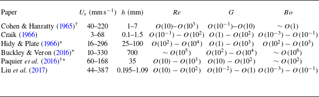
 Re=ρ2Ush2/μ2
 G=gh2/Us2
 Bo=ρ2gh22/T
 Us
Us g
g T
T ρ2
ρ2 μ2
μ2 h2
h2 Us
Us 2%
2%
 a
a a∈[1,∞)
 a∈(0,1)
 a∈[−1,0]
 a∈(−∞,−1]
 G
G a
a U(z)
U(z) a
a G=0
G=0 cr
cr ci
ci k
k a
a ci
ci a
a
 kmin
kmin (G,a)
(G,a) kmin>3
 kmin<3
 G=0.02
 cr
cr ci
ci k
k a
a a
a
 kci
kci (a,k)
(a,k) G=
G= 10−10
10−10 Ω/Ωmax
 G=0
G=0 a=−3
a=−3 k=6.31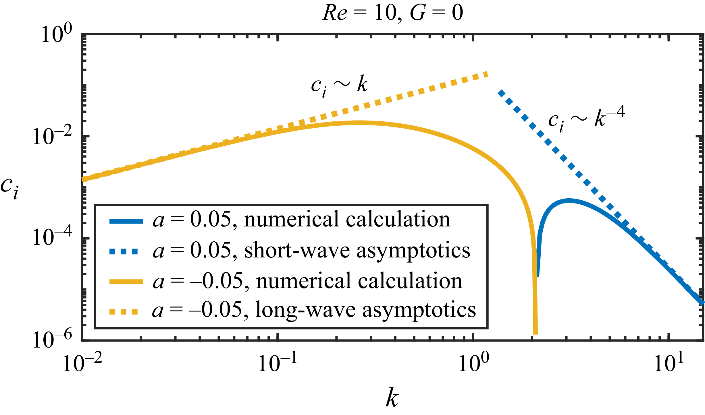
 ci
ci k
k a=0.05
 a=−0.05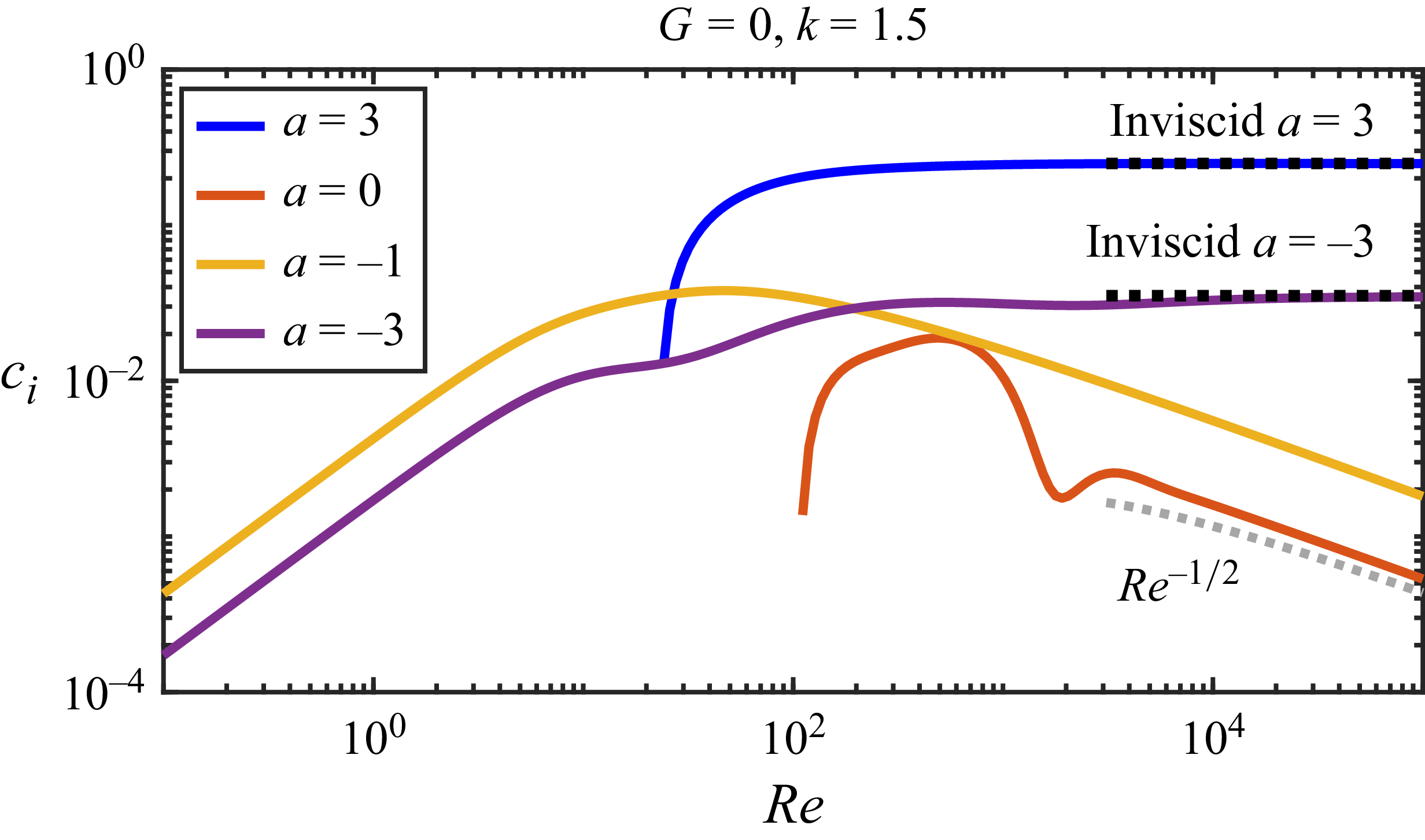
 ci
ci Re
Re a=3
a=3 a=0
a=0 a=−1
a=−1 a=−3
a=−3 a=3
a=3 a=−3
a=−3 Re−1/2
 a=0
a=0
 G=0
G=0 a=3
a=3 ci
ci Re
Re k
k kRe
kRe 0.1
0.1 0.5
0.5 1.5
1.5 ci
ci Re=1
Re=1 Re=105
 k=0.01
 k=0.02
 k=0.05
 k=0.1
k=0.1 kRe
kRe
 kci
kci k
k Re
Re a=−3
a=−3 a=−1
a=−1 a=0
a=0 a=3
a=3 G=0
G=0 G=0.02
 ×
×
 ε=(REY−TAN)/max(REY,TAN)
 (k,Re)
 G=0
G=0 a=
a= 3
3 −3
−3 −1
−1 0
0 k
k Re
Re cr=U(zc)
 zc
zc <0
<0 a=−1
a=−1 0
0 ε=−1
ε=−1
 Ω/Ωmax
 G=0
G=0 a=3
a=3 Re=1
Re=1 Re=105
 k=0.01
 Re=1
Re=1 Re=105
 Re=∞
Re=∞ k=20
k=20
 Ω/Ωmax
 G=0,a=0
 (k,Re)=
 1,103
1,103 6,103
6,103 1.75,150
 ×
×
 Ω/Ωmax
 G=0
G=0 Re=104
 k=0.1
k=0.1 k=1
k=1 k=10
k=10 a=3
a=3 k=0.1
k=0.1 k=1
k=1 k=10
k=10 a=−1
a=−1
 (k,Re)
 (a,Re)
 ci
ci k
k a=0.1
a=0.1 G=0,0.02
 0.5
0.5 ci
ci
 a=0
a=0 G=0
G=0
 Open access

