


I. Introduction
An important determinant of the net present value (NPV) of an investment project is its scalability. Even if the marginal profitability on a project is large at a small scale, when the profitability deteriorates quickly with size, agents will choose not to commit much capital to such projects, and, in the presence of fixed costs, may choose to forgo them altogether. Despite the importance of scalability, surprisingly little empirical work has quantitatively evaluated how important its cross-sectional variation is for capital allocation. In this article, we fill this void by focusing on the mutual fund market, where measuring the scalability of investment strategies has become commonplace.Footnote 1 In particular, the literature has argued that decreasing returns to scale (DRS) play a key role in equilibrating the mutual fund market.Footnote 2 Consistent with this argument, we show that scalability is an important driver of investors’ capital allocation decisions by exploiting heterogeneity across funds in DRS parameters: steeper DRS attenuate flow sensitivity to performance (FSP). Further, we calibrate a rational model of active fund management and show that 58% of the cross-sectional variation in fund size can plausibly be attributed to heterogeneity in DRS.
Our approach closely follows the insights from Berk and Green (Reference Berk and Green2004). As the percentage fees charged by funds change infrequently, equilibration operates primarily through their size (or assets under management (AUM)). When a fund outperforms, investors rationally learn that the fund is a positive NPV investment at its current size. In turn, flows go to that fund, eroding this positive NPV due to decreasing returns to scale: as the fund grows, its manager finds it increasingly difficult to put the new inflows to good use, leading to a deterioration of the fund’s performance. The inflows will stop when the fund is no longer a positive NPV investment opportunity, and its abnormal return to investors has reverted to zero.
We inspect this equilibrating mechanism more closely by formally deriving, in the context of the Berk and Green model, the relation between DRS and FSP: as a fund’s returns decrease in scale more steeply (steeper DRS), the positive net alpha is competed away with a smaller amount of capital inflows, making flows less sensitive to performance (weaker FSP).
To test this theoretical insight, one needs a source of variation in DRS in addition to observing investor reactions to this variation. We demonstrate that there is a substantial amount of heterogeneity in DRS across individual funds, with correspondingly heterogeneous FSP across funds. Our approach can be interpreted as inferring how the subjective size-performance relation, perceived by investors in real time, is incorporated into the flow-performance relation going forward. Consistent with our hypothesis, we find that a steeper DRS parameter predicts a lower FSP.
The main challenge in estimating the effect of DRS on FSP is the estimation error in fund-specific DRS (from fund-by-fund regressions), which is likely to induce attenuation bias in the point estimates of the DRS-FSP relation. Indeed, adjusting these DRS-FSP relation estimates for the errors-in-variable bias under the classical measurement error assumption—the errors are independent of the actual DRS—suggests that they are biased toward zero.
To address this issue, we estimate the DRS-FSP relation by instrumenting for the heterogeneity in DRS with a set of fund characteristics that are plausibly related to the scalability of investment strategies.Footnote 3 In particular, by regressing the fund-specific DRS estimates on these characteristics, we obtain fitted values that we use as a more robust way of obtaining cross-sectional variation. Importantly, we show that, while the characteristics-based estimates of the DRS-FSP relation remain statistically significant, they become substantially more negative, comparable in magnitude to those implied by the classical measurement error assumption. This result suggests that the characteristics-based approach is able to alleviate the errors-in-variables problem.
Next, we turn to the economic significance of our estimates. In particular, we assess how equilibrium fund size is affected by the cross-sectional variation in DRS parameters. This exercise does require model assumptions. We calibrate a rational model in the spirit of Berk and Green (Reference Berk and Green2004). After simulating data in which investors know the DRS can vary by fund, we check how much of the simulated size can be explained by counterfactual fund sizes computed under the assumption that investors believe the DRS is the same for all funds. We find that, on average, more than half (58%) of the variance of fund sizes across funds and periods can be related to cross-sectional variation in DRS parameters. Importantly, although we do not target the DRS-FSP relation in our calibration, our model produces DRS-FSP relation estimates that are quantitatively similar to those estimated from the actual data. Thus, the model does a good job of approximating the observed equilibrium in the mutual fund market.
Beyond implications for fund flows, the degree of DRS also has implications for fund size. In the model, fund size is directly proportional to the ratio of perceived skill to perceived scalability: all else equal (holding the alpha earned on the first dollar fixed), the DRS parameter should be lower for larger funds. This prediction is confirmed in our empirical analysis. Moreover, if investors learn about funds as in the model, the (log) fund size should converge to the (log) optimal size—the ratio of true skill to true scalability—as funds grow older. In Appendix D, we provide empirical evidence consistent with this prediction: the estimated optimal size largely explains capital allocation across older funds in the data. The size of older funds remains significantly related to their estimated optimal size, even when we control for an alternative proxy for optimal size that ignores cross-sectional heterogeneity in DRS. Again, investors seem to account for not only the average DRS but also the heterogeneity of DRS across funds.
Taken together, our results demonstrate that investors do account for the adverse effects of fund scale in making their capital allocation decisions.Footnote 4 The previous literature has often deemed mutual fund investors as naive return chasers because fund flows respond to past performance, although performance is not persistent,Footnote 5 and because funds show little evidence of outperformance.Footnote 6 In contrast, Berk and Green (Reference Berk and Green2004) argue that they are consistent with a model of how competition between rational investors determines the net alpha in equilibrium. We contribute to this debate by presenting findings that are hard to reconcile with anything other than the existence of rational fund flows.
Closely related to our article is Barras et al. (Reference Barras, Gagliardini and Scaillet2022), who also find that both skill and scalability—the degree of fund-level DRS—vary substantially across funds. They find that the majority of funds add value, consistent with rational equilibrium models of active mutual fund management. In contrast, we propose scalability as a key determinant of the flow-performance relation based on such models,Footnote 7 a hypothesis that we test by exploiting the fact that scalability varies substantially across funds. Furthermore, contrary to their analysis, we quantify the importance of cross-sectional variation in DRS for capital allocation decisions.
II. Definitions and Hypothesis
Let $ {R}_{it}^n $
denote the return in excess of the risk-free rate earned by fund
$ {R}_{it}^n $
denote the return in excess of the risk-free rate earned by fund $ i $
’s investors at time
$ i $
’s investors at time $ t $
and let
$ t $
and let $ {R}_{it}^B $
denote the excess return of the manager’s benchmark over the same time interval. At times
$ {R}_{it}^B $
denote the excess return of the manager’s benchmark over the same time interval. At times $ t $
, the investor observes the manager’s net return outperformance,
$ t $
, the investor observes the manager’s net return outperformance,
 $$ {\alpha}_{it+1}\equiv {R}_{it}^n-{R}_{it}^B. $$
We assume throughout that $ {\alpha}_{it} $
can be expressed as follows:
$ {\alpha}_{it} $
can be expressed as follows:
 $$ {\alpha}_{it}={a}_i-{b}_ih\left({q}_{it-1}\right)+{\unicode{x025B}}_{it}, $$
where $ {q}_{it-1} $
denotes the size (i.e., real AUM) of fund
$ {q}_{it-1} $
denotes the size (i.e., real AUM) of fund $ i $
at time
$ i $
at time $ t-1 $
,
$ t-1 $
, $ {a}_i $
denotes a parameter that captures fund
$ {a}_i $
denotes a parameter that captures fund $ i $
’s gross alpha on the first dollar net of the percentage fee its manager charges, and
$ i $
’s gross alpha on the first dollar net of the percentage fee its manager charges, and $ {\unicode{x025B}}_{it} $
is the noise in observed performance. Here
$ {\unicode{x025B}}_{it} $
is the noise in observed performance. Here $ {b}_ih(q) $
captures the DRS the manager faces, which can vary by fund:
$ {b}_ih(q) $
captures the DRS the manager faces, which can vary by fund: $ {b}_i>0 $
is a parameter that captures the cross-sectional variation in DRS technology. For the form of DRS technology, we use the logarithmic specification (
$ {b}_i>0 $
is a parameter that captures the cross-sectional variation in DRS technology. For the form of DRS technology, we use the logarithmic specification ( $ h(q)=\log (q) $
) commonly used in empirical studies for simplicity in the rest of the article and provide a necessary and sufficient condition on the DRS technology for our hypothesis (Proposition 1) in Appendix A.Footnote
8
$ h(q)=\log (q) $
) commonly used in empirical studies for simplicity in the rest of the article and provide a necessary and sufficient condition on the DRS technology for our hypothesis (Proposition 1) in Appendix A.Footnote
8
Now note that $ {\alpha}_{it} $
is an informative signal about
$ {\alpha}_{it} $
is an informative signal about $ {a}_i $
: high
$ {a}_i $
: high $ {\alpha}_{it} $
implies good news about
$ {\alpha}_{it} $
implies good news about $ {a}_i $
and low
$ {a}_i $
and low $ {\alpha}_{it} $
implies bad news about
$ {\alpha}_{it} $
implies bad news about $ {a}_i $
. Thus, at time t, investors use the time-t information set
$ {a}_i $
. Thus, at time t, investors use the time-t information set $ {I}_t $
to update their beliefs on
$ {I}_t $
to update their beliefs on $ {a}_i $
implying that the expectation of
$ {a}_i $
implying that the expectation of $ {a}_i $
at time t is as follows:
$ {a}_i $
at time t is as follows:
 $$ {\theta}_{it}\equiv E\left[{a}_i\left|{I}_t\right.\right]. $$
Let $ {\overline{\alpha}}_{it}(q) $
denote investors’ subjective expectation of
$ {\overline{\alpha}}_{it}(q) $
denote investors’ subjective expectation of $ {\alpha}_{it+1} $
when fund i has size q at time t (i.e., fund
$ {\alpha}_{it+1} $
when fund i has size q at time t (i.e., fund $ i $
’s net alpha):
$ i $
’s net alpha):
 $$ {\overline{\alpha}}_{it}(q)={\theta}_{it}-{b}_ih(q). $$
In equilibrium, the size of the fund $ {q}_{it} $
adjusts to ensure that there are no positive NPV investment opportunities so
$ {q}_{it} $
adjusts to ensure that there are no positive NPV investment opportunities so $ {\overline{\alpha}}_{it}\left({q}_{it}\right)=0 $
and
$ {\overline{\alpha}}_{it}\left({q}_{it}\right)=0 $
and
 $$ \frac{\theta_{it}}{b_i}=h\left({q}_{it}\right)=\log \left({q}_{it}\right). $$
Following Berk and Green (Reference Berk and Green2004), we assume in the rest of the article that i) investors’ prior is that $ {a}_i $
is normally distributed with mean
$ {a}_i $
is normally distributed with mean $ {\theta}_{i0} $
and variance
$ {\theta}_{i0} $
and variance $ {\sigma}_0^2 $
, and ii)
$ {\sigma}_0^2 $
, and ii) $ {\unicode{x025B}}_{it} $
is normally distributed with mean zero and variance
$ {\unicode{x025B}}_{it} $
is normally distributed with mean zero and variance $ {\sigma}_{\unicode{x025B}}^2 $
, but we relax these assumptions in Appendix A.Footnote
9 Then, it is straightforward that the mean of investors’ posteriors satisfies the following recursion:
$ {\sigma}_{\unicode{x025B}}^2 $
, but we relax these assumptions in Appendix A.Footnote
9 Then, it is straightforward that the mean of investors’ posteriors satisfies the following recursion:
 $$ {\theta}_{it}={\theta}_{it-1}+\frac{\sigma_0^2}{\sigma_{\unicode{x025B}}^2+t{\sigma}_0^2}{\alpha}_{it}. $$
Next, let the flow of capital into the mutual fund $ i $
at time
$ i $
at time $ t $
be denoted:
$ t $
be denoted:
 $$ {F}_{it}\equiv \log \left({q}_{it}/{q}_{it-1}\right)=\frac{\theta_{it}-{\theta}_{it-1}}{b_i}=\frac{\sigma_0^2}{\sigma_{\unicode{x025B}}^2+t{\sigma}_0^2}\frac{\alpha_{it}}{b_i}, $$
where the first equality follows from (5) and the last equality follows from (6). Differentiating this expression with respect to $ {\alpha}_{it} $
,
$ {\alpha}_{it} $
,
 $$ \frac{\partial {F}_{it}}{\partial {\alpha}_{it}}=\frac{\sigma_0^2}{\sigma_{\unicode{x025B}}^2+t{\sigma}_0^2}\frac{1}{b_i}>0, $$
so good (bad) performance results in an inflow (outflow) of funds. This result is one of the important insights from Berk and Green (Reference Berk and Green2004).
Taking the derivative of the flow-performance sensitivity with respect to $ {b}_i $
, we see that steeper DRS leads to a weaker FSP:
$ {b}_i $
, we see that steeper DRS leads to a weaker FSP:
 $$ \frac{\partial }{\partial {b}_i}\left(\frac{\partial {F}_{it}}{\partial {\alpha}_{it}}\right)=-\frac{\sigma_0^2}{\sigma_{\unicode{x025B}}^2+t{\sigma}_0^2}\frac{1}{b_i^2}<0. $$
This leads to the following proposition, which will be our main hypothesis that we take to the data:
Proposition 1. Steeper DRS leads to a weaker FSP.
Intuitively, as a fund’s returns decrease in scale more steeply (steeper DRS), the positive net alpha is competed away with a smaller amount of capital inflows, making flows less sensitive to performance (weaker FSP).Footnote 10
Remark 1. Note that the scalability parameter is assumed to be constant for a given fund, but this assumption is not essential for Proposition 1. If the scalability parameter is time-varying—with $ {b}_{it} $
denoting the true DRS fund
$ {b}_{it} $
denoting the true DRS fund $ i $
faces at time
$ i $
faces at time $ t $
—it is straightforward to show that the derivative (8) becomes
$ t $
—it is straightforward to show that the derivative (8) becomes
 $$ \frac{\partial }{\partial {b}_{it}}\left(\frac{\partial {F}_{it}}{\partial {\alpha}_{it}}\right)=-\frac{\sigma_0^2}{\sigma_{\unicode{x025B}}^2+t{\sigma}_0^2}\frac{1}{b_{it}^2}<0, $$
so steeper DRS still leads to a weaker FSP.
Remark 2. Note that the scalability of a fund is implicitly assumed to be known by investors, as in much of the earlier literature, but this assumption is not essential for Proposition 1.Footnote
11 If the scalability parameter obeys an AR(1) process—with $ {b}_{it}={\phi}_0+{\phi}_1{b}_{it-1}+{\eta}_{it} $
—and investors’ prior that
$ {b}_{it}={\phi}_0+{\phi}_1{b}_{it-1}+{\eta}_{it} $
—and investors’ prior that $ {a}_i $
and
$ {a}_i $
and $ {b}_{it} $
follows a bivariate normal distribution, it is straightforward to show that the derivative (8) becomes
$ {b}_{it} $
follows a bivariate normal distribution, it is straightforward to show that the derivative (8) becomes
 $$ \frac{\partial }{\partial {\hat{b}}_{it}}\left(\frac{\partial {F}_{it}}{\partial {\alpha}_{it}}\right)=-\frac{\frac{\partial {\theta}_{it}}{\partial {\alpha}_{it}}-2\log \left({q}_{it}\right)\frac{\partial {\hat{b}}_{it}}{\partial {\alpha}_{it}}}{{\hat{b}}_{it}^2}, $$
where $ {\displaystyle \begin{array}{l}\frac{\partial {\theta}_{it}}{\partial {\alpha}_{it}}=\frac{{\mathrm{Var}}_{t-1}\left({a}_i\right)-{\operatorname{cov}}_{t-1}\left({a}_i,{b}_{it-1}\right)\log \left({q}_{it-1}\right)}{{\mathrm{Var}}_{t-1}\left({\alpha}_{it}\right)}\\ {}\frac{\partial {\hat{b}}_{it}}{\partial {\alpha}_{it}}=-{\phi}_1\frac{{\mathrm{Var}}_{t-1}\left({b}_{it-1}\right)\log \left({q}_{it-1}\right)-{\operatorname{cov}}_{t-1}\left({a}_i,{b}_{it-1}\right)}{{\mathrm{Var}}_{t-1}\left({\alpha}_{it}\right)}\end{array}} $
The derivative in equation (10) is negative under two sufficient conditions: i) the conditional covariance cov $ {}_{t-1}\left({a}_i,{b}_{it-1}\right) $
is sufficiently small and ii) both
$ {}_{t-1}\left({a}_i,{b}_{it-1}\right) $
is sufficiently small and ii) both $ {\theta}_{it} $
and
$ {\theta}_{it} $
and $ {\theta}_{it-1} $
are sufficiently large. The first condition implies that investors interpret strong performance as a signal of both higher-than-expected skill (
$ {\theta}_{it-1} $
are sufficiently large. The first condition implies that investors interpret strong performance as a signal of both higher-than-expected skill ( $ {\theta}_{it}>{\theta}_{it-1} $
) and better-than-expected scalability (
$ {\theta}_{it}>{\theta}_{it-1} $
) and better-than-expected scalability ( $ {\hat{b}}_{it}\le $
E
$ {\hat{b}}_{it}\le $
E $ {}_{t-1}\left({b}_{it}\right) $
). If, instead, investors believe a priori that skill and scalability are tightly positively correlated, they may interpret superior performance as a sign of lower skill or worse scalability, resulting in a negative flow-performance relation. The second condition is likely to hold in practice, since funds face fixed operating costs and will optimally exit when they can no longer cover these costs. This behavior naturally bounds
$ {}_{t-1}\left({b}_{it}\right) $
). If, instead, investors believe a priori that skill and scalability are tightly positively correlated, they may interpret superior performance as a sign of lower skill or worse scalability, resulting in a negative flow-performance relation. The second condition is likely to hold in practice, since funds face fixed operating costs and will optimally exit when they can no longer cover these costs. This behavior naturally bounds $ {\theta}_{it} $
and
$ {\theta}_{it} $
and $ {\theta}_{it-1} $
comes from below. In sum, even when the scalability parameter is time-varying and unobservable, steeper DRS (perceived by investors in real time) still lead to a weaker FSP under empirically plausible conditions.
$ {\theta}_{it-1} $
comes from below. In sum, even when the scalability parameter is time-varying and unobservable, steeper DRS (perceived by investors in real time) still lead to a weaker FSP under empirically plausible conditions.
III. Data
Our data come from CRSP and Morningstar. We require that funds appear in both the CRSP and Morningstar databases, which allows us to validate data accuracy across the two. We merge CRSP and Morningstar based on funds’ tickers, CUSIPs, and names. We then compare assets and returns across the two sources in an effort to check the accuracy of each match following Berk and van Binsbergen (Reference Berk and van Binsbergen2015) and Pástor, Stambaugh, and Taylor (Reference Stambaugh and Taylor2015). We refer the readers to the data appendices of those papers for the details. Our mutual fund data set contains 3,066 actively managed domestic equity-only mutual funds in the United States between 1991 and 2014.Footnote 12 Finally, we drop any fund observations before the fund’s (inflation-adjusted) AUM reaches $5 million.
We now define the key variables used in our empirical analysis: fund performance, fund size, and fund flows. Summary statistics are in Table 1.

A. Fund Performance
We take two approaches to measuring fund performance. First, we use the standard risk-based approach. The recent literature finds that investors use the CAPM in making their capital allocation decisions (Berk and van Binsbergen (Reference Berk and van Binsbergen2016), Barber, Huang, and Odean (Reference Barber, Huang and Odean2016)), so we adopt the CAPM. In this case, the risk adjustment $ {R}_{it}^{\mathrm{CAPM}} $
is given by:
$ {R}_{it}^{\mathrm{CAPM}} $
is given by:
 $$ {R}_{it}^{\mathrm{CAPM}}={\beta}_{it}{\mathrm{MKT}}_t, $$
where MKT $ {}_t $
is the realized market excess return and
$ {}_t $
is the realized market excess return and $ {\beta}_{it} $
is the market beta of the fund
$ {\beta}_{it} $
is the market beta of the fund $ i $
. We estimate
$ i $
. We estimate $ {\beta}_{it} $
by regressing the fund’s excess return to investors onto the market portfolio over the 60 months prior to the month
$ {\beta}_{it} $
by regressing the fund’s excess return to investors onto the market portfolio over the 60 months prior to the month $ t $
. To produce reliable beta estimates, we require a fund to have at least 2 years of track record to estimate its betas from the rolling window regressions.
$ t $
. To produce reliable beta estimates, we require a fund to have at least 2 years of track record to estimate its betas from the rolling window regressions.
Second, we follow Berk and van Binsbergen (Reference Berk and van Binsbergen2015) by taking the set of available Vanguard index funds as the alternative investment opportunity set,Footnote
13 so the benchmark of a fund is defined as the closest portfolio in that set to it. Let $ {R}_t^j $
denote the excess return earned by investors in the
$ {R}_t^j $
denote the excess return earned by investors in the $ j $
’th Vanguard index fund at time
$ j $
’th Vanguard index fund at time $ t $
. Then the benchmark return for fund
$ t $
. Then the benchmark return for fund $ i $
is given by the following equation:
$ i $
is given by the following equation:
 $$ {R}_{it}^{\mathrm{VG}}=\sum \limits_{j=1}^{n(t)}{\beta}_i^j{R}_t^j, $$
where $ n(t) $
is the number of Vanguard index funds available at time
$ n(t) $
is the number of Vanguard index funds available at time $ t $
and
$ t $
and $ {\beta}_i^j $
is obtained from the appropriate linear projection of fund
$ {\beta}_i^j $
is obtained from the appropriate linear projection of fund $ i $
onto the set of Vanguard index funds. As pointed out by Berk and van Binsbergen (Reference Berk and van Binsbergen2015), using Vanguard funds as the benchmark ensures that this alternative investment opportunity set was marketed and tradable at the time. Again, we require a fund to have at least 24 months of data to estimate its projection coefficients (
$ i $
onto the set of Vanguard index funds. As pointed out by Berk and van Binsbergen (Reference Berk and van Binsbergen2015), using Vanguard funds as the benchmark ensures that this alternative investment opportunity set was marketed and tradable at the time. Again, we require a fund to have at least 24 months of data to estimate its projection coefficients ( $ {\beta}_i^j $
) used to calculate the Vanguard benchmark for fund
$ {\beta}_i^j $
) used to calculate the Vanguard benchmark for fund $ i $
.
$ i $
.
Our measures of fund performance are then $ {\hat{\alpha}}_{it}^{\mathrm{CAPM}} $
and
$ {\hat{\alpha}}_{it}^{\mathrm{CAPM}} $
and $ {\hat{\alpha}}_{it}^{\mathrm{VG}} $
, the realized return for the fund in month
$ {\hat{\alpha}}_{it}^{\mathrm{VG}} $
, the realized return for the fund in month $ t $
less
$ t $
less $ {\hat{R}}_{it}^{\mathrm{CAPM}} $
and
$ {\hat{R}}_{it}^{\mathrm{CAPM}} $
and $ {\hat{R}}_{it}^{\mathrm{VG}} $
, respectively. The average
$ {\hat{R}}_{it}^{\mathrm{VG}} $
, respectively. The average $ {\hat{\alpha}}_{it}^{\mathrm{CAPM}} $
is
$ {\hat{\alpha}}_{it}^{\mathrm{CAPM}} $
is $ +1.0 $
basis points per month, while the average
$ +1.0 $
basis points per month, while the average $ {\hat{\alpha}}_{it}^{\mathrm{VG}} $
is
$ {\hat{\alpha}}_{it}^{\mathrm{VG}} $
is $ -1.7 $
basis points per month.
$ -1.7 $
basis points per month.
B. Fund Size and Flows
We adjust all AUM numbers by inflation by expressing them in Jan. 1, 2000 dollars. Adjusting AUM by inflation reflects the notion that the fund’s real (rather than nominal) size is relevant for capturing DRS in active management—lagged real AUM corresponds to $ {q}_{it-1} $
in the model from Section II. There is considerable dispersion in real AUM: the inner-quartile range is from $44 million to $621 million, while the 99th percentile is orders of magnitude larger at $16 billion.
$ {q}_{it-1} $
in the model from Section II. There is considerable dispersion in real AUM: the inner-quartile range is from $44 million to $621 million, while the 99th percentile is orders of magnitude larger at $16 billion.
Flows are measured in two different ways. First, as in the model, we define fund flow $ F $
as the logarithmic change in real AUM—the percentage change in fund size. Alternatively, we calculate flows for fund
$ F $
as the logarithmic change in real AUM—the percentage change in fund size. Alternatively, we calculate flows for fund $ i $
in month
$ i $
in month $ t $
as:
$ t $
as:
 $$ {F}_{it}=\frac{AUM_{it}-{AUM}_{it-1}\left(1+{R}_{it}\right)}{AUM_{it-1}\left(1+{R}_{it}\right)}, $$
where $ {AUM}_{it} $
is fund
$ {AUM}_{it} $
is fund $ i $
’s nominal AUM at the end of month
$ i $
’s nominal AUM at the end of month $ t $
, and
$ t $
, and $ {R}_{it} $
is fund
$ {R}_{it} $
is fund $ i $
’s total return in month
$ i $
’s total return in month $ t $
.Footnote
14 Under this more standard definition
$ t $
.Footnote
14 Under this more standard definition $ F $
, flows represent the percentage change in new assets. The flow of fund data contain some implausible outliers, so we winsorize the two flow variables at their 1st and 99th percentiles. Mean monthly changes in fund size and in new assets are
$ F $
, flows represent the percentage change in new assets. The flow of fund data contain some implausible outliers, so we winsorize the two flow variables at their 1st and 99th percentiles. Mean monthly changes in fund size and in new assets are $ 0.8\% $
and
$ 0.8\% $
and $ 0.5\% $
, respectively.
$ 0.5\% $
, respectively.
IV. Method
Our analysis relies on a theoretical link between DRS and FSP. We discuss how we estimate each part in the following sections.
A. Fund-Specific DRS
Empirically, the net alpha earned by fund $ i $
’s investors in month
$ i $
’s investors in month $ t $
is given by the following equation:
$ t $
is given by the following equation:
 $$ {\alpha}_{it}={a}_i-{b}_i\log \left({q}_{it-1}\right)+{\unicode{x025B}}_{it}, $$
where $ {a}_i $
is the fund fixed effect,
$ {a}_i $
is the fund fixed effect, $ {b}_i $
captures the size effect, which can vary by fund, and
$ {b}_i $
captures the size effect, which can vary by fund, and $ {q}_{it-1} $
is the fund’s lagged real AUM.Footnote
15 This simple regression model corresponds to the model in Section II.
$ {q}_{it-1} $
is the fund’s lagged real AUM.Footnote
15 This simple regression model corresponds to the model in Section II.
We depart from much of the literature by allowing for heterogeneity in the size-performance relation across funds. Indeed, the effect of scale on a fund’s performance is unlikely to be constant across funds. For example, a fund’s returns should decrease in scale more steeply for those that invest in small and illiquid stocks.
We start our analysis by estimating fund-specific $ {b}_i $
parameters. It is well known that the OLS estimators of
$ {b}_i $
parameters. It is well known that the OLS estimators of $ {b}_i $
in (11) are subject to a small-sample bias (Stambaugh (Reference Stambaugh1999)). The small-sample bias arises because changes in fund size tend to be positively correlated with unexpected fund returns. To address this bias, we follow Amihud and Hurvich (Reference Amihud and Hurvich2004) and Barras et al. (Reference Barras, Gagliardini and Scaillet2022) and include a proxy for the size innovation
$ {b}_i $
in (11) are subject to a small-sample bias (Stambaugh (Reference Stambaugh1999)). The small-sample bias arises because changes in fund size tend to be positively correlated with unexpected fund returns. To address this bias, we follow Amihud and Hurvich (Reference Amihud and Hurvich2004) and Barras et al. (Reference Barras, Gagliardini and Scaillet2022) and include a proxy for the size innovation $ {v}_{i\tau}^c $
(see Appendix C):Footnote
16 for each fund
$ {v}_{i\tau}^c $
(see Appendix C):Footnote
16 for each fund $ i $
at time
$ i $
at time $ t $
, we define the fund-specific DRS estimate
$ t $
, we define the fund-specific DRS estimate $ {\hat{b}}_{it} $
to be the coefficient of
$ {\hat{b}}_{it} $
to be the coefficient of $ -\log \left({q}_{i\tau -1}\right) $
in the time-series regression of
$ -\log \left({q}_{i\tau -1}\right) $
in the time-series regression of $ {\hat{\alpha}}_{i\tau} $
on
$ {\hat{\alpha}}_{i\tau} $
on $ -\log \left({q}_{i\tau -1}\right) $
and
$ -\log \left({q}_{i\tau -1}\right) $
and $ {v}_{i\tau}^c $
(including an intercept) using 60 months of data before time
$ {v}_{i\tau}^c $
(including an intercept) using 60 months of data before time $ t $
. We require at least 3 years of data to estimate fund-specific DRS of a fund.
$ t $
. We require at least 3 years of data to estimate fund-specific DRS of a fund.
Intuitively, the estimate of $ {b}_i $
,
$ {b}_i $
, $ {\hat{b}}_{it} $
, represents investors’ perception of the effect of size on performance for fund
$ {\hat{b}}_{it} $
, represents investors’ perception of the effect of size on performance for fund $ i $
at time
$ i $
at time $ t $
based on information prior to time
$ t $
based on information prior to time $ t $
. Graph A of Figure 1 shows how the cross-sectional distribution of
$ t $
. Graph A of Figure 1 shows how the cross-sectional distribution of $ {\hat{b}}_{it} $
using the CAPM alpha varies over time. For each month in 1991 through 2014, the figure plots the average as well as the percentiles of the estimated fund-specific b parameters across all funds in that month. The plot shows considerable heterogeneity in DRS across fundsFootnote
17: the interquartile range is more than 4 times larger than the estimates’ cross-sectional median. We find that, for the average fund, a 1% increase in fund size is associated with a sizeable decrease in performance of about 0.4 basis points per month. This evidence suggests that the subjective size-performance relation, perceived by investors in real time, provides identifying variation in the extent of DRS.
$ {\hat{b}}_{it} $
using the CAPM alpha varies over time. For each month in 1991 through 2014, the figure plots the average as well as the percentiles of the estimated fund-specific b parameters across all funds in that month. The plot shows considerable heterogeneity in DRS across fundsFootnote
17: the interquartile range is more than 4 times larger than the estimates’ cross-sectional median. We find that, for the average fund, a 1% increase in fund size is associated with a sizeable decrease in performance of about 0.4 basis points per month. This evidence suggests that the subjective size-performance relation, perceived by investors in real time, provides identifying variation in the extent of DRS.
Figure 1 displays how the cross-sectional distribution of $ {\hat{b}}_{it} $
(fund i’s DRS estimated using 60 months of data before month t) varies over time. Graph A shows the plot when fund-specific DRS is estimated using the CAPM, and Graph B shows the plot using Vanguard index funds as benchmark portfolios.
$ {\hat{b}}_{it} $
(fund i’s DRS estimated using 60 months of data before month t) varies over time. Graph A shows the plot when fund-specific DRS is estimated using the CAPM, and Graph B shows the plot using Vanguard index funds as benchmark portfolios.

Graph B of Figure 1 shows how the cross-sectional distribution of $ {\hat{b}}_{it} $
varies over time when we estimate fund-specific DRS using
$ {\hat{b}}_{it} $
varies over time when we estimate fund-specific DRS using $ {\hat{\alpha}}_{it}^{\mathrm{VG}} $
. Similar to when we use the CAPM alpha to estimate
$ {\hat{\alpha}}_{it}^{\mathrm{VG}} $
. Similar to when we use the CAPM alpha to estimate $ {\hat{b}}_{it} $
in Graph A, this plot shows considerable heterogeneity in DRS across funds, although these estimates typically indicate milder DRS.
$ {\hat{b}}_{it} $
in Graph A, this plot shows considerable heterogeneity in DRS across funds, although these estimates typically indicate milder DRS.
B. Fund-Specific FSP
We estimate the fund-specific FSPs by estimating the following regression fund-by-fund:
 $$ {F}_{it}={c}_i+{\gamma}_i{P}_{it-1}+{\upsilon}_{it}, $$
where $ {P}_{it-1} $
is annual alpha for the year leading to month
$ {P}_{it-1} $
is annual alpha for the year leading to month $ t-1 $
, computed by compounding the monthly alphas. This regression is consistent with empirical evidence that investors do not respond immediately.Footnote
18 Parameter
$ t-1 $
, computed by compounding the monthly alphas. This regression is consistent with empirical evidence that investors do not respond immediately.Footnote
18 Parameter $ {\gamma}_i>0 $
captures the positive time-series relation between performance and fund flows, which can vary by fund.
$ {\gamma}_i>0 $
captures the positive time-series relation between performance and fund flows, which can vary by fund.
For each fund $ i $
at time
$ i $
at time $ t $
, we calculate the fund’s FSP by estimating (12) using its data over the subsequent 5 years. Let
$ t $
, we calculate the fund’s FSP by estimating (12) using its data over the subsequent 5 years. Let $ {\hat{FSP}}_{it} $
be the flow-performance sensitivity estimate from that model. We require these coefficient estimates to be obtained from at least 3 years of data. For the average fund, we observe that an increase in
$ {\hat{FSP}}_{it} $
be the flow-performance sensitivity estimate from that model. We require these coefficient estimates to be obtained from at least 3 years of data. For the average fund, we observe that an increase in $ 1\% $
in the annual CAPM alpha is associated with a
$ 1\% $
in the annual CAPM alpha is associated with a $ 0.1\% $
increase in monthly flows next month.
$ 0.1\% $
increase in monthly flows next month.
Graph A of Figures 2 and 3 displays the evolution of the $ {\hat{FSP}}_{it} $
distributions over time, measuring flows as percentage changes in fund size and in new assets, respectively. Both plots manifest considerable heterogeneities in the flow-performance relation across funds. Moreover, these plots show that while the average
$ {\hat{FSP}}_{it} $
distributions over time, measuring flows as percentage changes in fund size and in new assets, respectively. Both plots manifest considerable heterogeneities in the flow-performance relation across funds. Moreover, these plots show that while the average $ {\hat{FSP}}_{it} $
do not exhibit any obvious trend, they are certainly time varying. Also noteworthy is the fact that the distributions remain roughly the same over our sample period, conditional on the median.
$ {\hat{FSP}}_{it} $
do not exhibit any obvious trend, they are certainly time varying. Also noteworthy is the fact that the distributions remain roughly the same over our sample period, conditional on the median.
Figure 2 displays the distributions of $ {\hat{FSP}}_{it} $
(the fund’s FSP estimated using its data over the subsequent 5 years) over time. Graph A shows the plot when fund-specific FSP is estimated using the CAPM, and Graph B shows the plot using Vanguard index funds as benchmark portfolios.
$ {\hat{FSP}}_{it} $
(the fund’s FSP estimated using its data over the subsequent 5 years) over time. Graph A shows the plot when fund-specific FSP is estimated using the CAPM, and Graph B shows the plot using Vanguard index funds as benchmark portfolios.

Figure 3 displays the distributions of $ {\hat{FSP}}_{it} $
(the fund’s FSP estimated using its data over the subsequent 5 years) over time. Graph A shows the plot when fund-specific FSP is estimated using the CAPM, and Graph B shows the plot using Vanguard index funds as benchmark portfolios.
$ {\hat{FSP}}_{it} $
(the fund’s FSP estimated using its data over the subsequent 5 years) over time. Graph A shows the plot when fund-specific FSP is estimated using the CAPM, and Graph B shows the plot using Vanguard index funds as benchmark portfolios.

Graph B of Figures 2 and 3 displays the evolution of the $ {\hat{FSP}}_{it} $
distributions over time when we estimate fund-specific FSP using
$ {\hat{FSP}}_{it} $
distributions over time when we estimate fund-specific FSP using $ {\hat{\alpha}}_{it}^{\mathrm{VG}} $
. Similar to when we use the CAPM alpha to estimate
$ {\hat{\alpha}}_{it}^{\mathrm{VG}} $
. Similar to when we use the CAPM alpha to estimate $ {\hat{FSP}}_{it} $
in Graph A, these plots manifest considerable heterogeneities in the flow-performance relation across funds.
$ {\hat{FSP}}_{it} $
in Graph A, these plots manifest considerable heterogeneities in the flow-performance relation across funds.
V. Results
A. DRS and FSP
To examine whether fund-specific DRS parameters affect capital allocation decisions, we run panel regressions of fund $ i $
’s FSP going forward in month
$ i $
’s FSP going forward in month $ t $
,
$ t $
, $ {\hat{FSP}}_{it} $
, on its DRS estimated as of the previous month-end,
$ {\hat{FSP}}_{it} $
, on its DRS estimated as of the previous month-end, $ {\hat{b}}_{it} $
. We test the null hypothesis that the slope on
$ {\hat{b}}_{it} $
. We test the null hypothesis that the slope on $ {\hat{b}}_{it} $
is 0.Footnote
19 We report the results based on raw estimates in Table 2.Footnote
20 In Panel A, we present results using estimates of fund-specific DRS and FSP based on the CAPM alpha, and in Panel B, we present results based on
$ {\hat{b}}_{it} $
is 0.Footnote
19 We report the results based on raw estimates in Table 2.Footnote
20 In Panel A, we present results using estimates of fund-specific DRS and FSP based on the CAPM alpha, and in Panel B, we present results based on $ {\hat{\alpha}}_{it}^{\mathrm{VG}} $
.
$ {\hat{\alpha}}_{it}^{\mathrm{VG}} $
.

We focus on variation in sensitivity coming from the market equilibrating mechanism by including both fund and month fixed effects. Fund fixed effects absorb variation in FSP, for example, due to cross-sectional differences in investor clientele,Footnote 21 or baseline fund scalability, while month fixed effects soak up variation in FSP due to factors like time-varying investor attention allocation.Footnote 22 Conceptually, we think the relationship between FSP and scalability in our regression models is driven by within-fund variation in perceived scalability over time: as investors update their beliefs by observing a fund’s returns and size, the fund’s perceived scalability fluctuates, leading to fluctuations in the flow sensitivity to the fund’s performance.
In the odd columns, we only include month and fund fixed effects. The results in Panel A are consistent with the main prediction of our model: the estimated coefficients on $ {\hat{b}}_{it} $
are significantly negative, with t-statistics of
$ {\hat{b}}_{it} $
are significantly negative, with t-statistics of $ -6.3 $
in column 1 and
$ -6.3 $
in column 1 and $ -3.0 $
in column 3. These findings are unaffected by including a host of controls in the even columns, where we add proxies for participation costs considered by Huang et al. (Reference Huang, Wei and Yan2007),Footnote
23 as well as performance volatility and fund age.Footnote
24 The slopes on
$ -3.0 $
in column 3. These findings are unaffected by including a host of controls in the even columns, where we add proxies for participation costs considered by Huang et al. (Reference Huang, Wei and Yan2007),Footnote
23 as well as performance volatility and fund age.Footnote
24 The slopes on $ {\hat{b}}_{it} $
remain negative and highly significant, with t-statistics of
$ {\hat{b}}_{it} $
remain negative and highly significant, with t-statistics of $ -7.1 $
in column 2 and
$ -7.1 $
in column 2 and $ -3.3 $
in column 4, and their magnitude increases.
$ -3.3 $
in column 4, and their magnitude increases.
In Panel B, the same conclusions continue to hold when we use estimates of fund-specific DRS and FSP based on $ {\hat{\alpha}}_{it}^{\mathrm{VG}} $
. Just like in Panel A, the estimated coefficients on
$ {\hat{\alpha}}_{it}^{\mathrm{VG}} $
. Just like in Panel A, the estimated coefficients on $ {\hat{b}}_{it} $
are significantly negative, and their magnitude increases when we include a host of controls.
$ {\hat{b}}_{it} $
are significantly negative, and their magnitude increases when we include a host of controls.
Table 3 repeats this exercise with percentile ranks in each month based on $ {\hat{b}}_{it} $
and
$ {\hat{b}}_{it} $
and $ {\hat{FSP}}_{it} $
. Now, we do not use month fixed effects: percentile ranks already control for time variation in the flow-performance relation. In each column, the estimated coefficient on
$ {\hat{FSP}}_{it} $
. Now, we do not use month fixed effects: percentile ranks already control for time variation in the flow-performance relation. In each column, the estimated coefficient on $ {\hat{b}}_{it} $
is significantly negative at the 1% confidence level.
$ {\hat{b}}_{it} $
is significantly negative at the 1% confidence level.

To summarize, we find a strong negative relation between DRS and FSP, consistent with the presence of investors rationally accounting for the adverse effects of fund scale in making their capital allocation decisions. Unfortunately, the coefficient values in Table 2 are likely biased toward zero because of the measurement error in $ {\hat{b}}_{it} $
. In Section V.A.1, we first gauge the severity of attenuation bias under the classical measurement error assumption. In Section V.A.2, we then exploit a set of fund characteristics that are plausibly related to the scalability of investment strategies as instruments for heterogeneity in DRS parameters across funds to address the attenuation bias associated with estimating the DRS-FSP relation. Finally, in Section V.A.3, we propose a way of assessing the economic magnitude of these estimated coefficients by computing counterfactual fund sizes.
$ {\hat{b}}_{it} $
. In Section V.A.1, we first gauge the severity of attenuation bias under the classical measurement error assumption. In Section V.A.2, we then exploit a set of fund characteristics that are plausibly related to the scalability of investment strategies as instruments for heterogeneity in DRS parameters across funds to address the attenuation bias associated with estimating the DRS-FSP relation. Finally, in Section V.A.3, we propose a way of assessing the economic magnitude of these estimated coefficients by computing counterfactual fund sizes.
1. DRS-FSP Relation Under the Classical Measurement Error Assumption
To gauge the severity of attenuation bias, we adjust the estimated coefficients on $ {\hat{b}}_{it} $
in Table 2 for the errors-in-variable (EIV) problem, assuming that the errors are of the classical type: they are purely random, mean zero, and uncorrelated with the regressors, including the actual
$ {\hat{b}}_{it} $
in Table 2 for the errors-in-variable (EIV) problem, assuming that the errors are of the classical type: they are purely random, mean zero, and uncorrelated with the regressors, including the actual $ {b}_i $
, and with the regression errors. Using the standard errors
$ {b}_i $
, and with the regression errors. Using the standard errors $ {\hat{b}}_{it} $
to estimate the variance of measurement error in
$ {\hat{b}}_{it} $
to estimate the variance of measurement error in $ {b}_i $
, we calculate the EIV-adjusted coefficients and their standard errors, reported in the last 2 rows of the panel.
$ {b}_i $
, we calculate the EIV-adjusted coefficients and their standard errors, reported in the last 2 rows of the panel.
As expected, the simple DRS-FSP relation estimates tend to be too small in magnitude. For example, when the DRS-FSP relation is estimated based on the CAPM controlling for other determinants of the flow-performance relation (column 2 of Panel A), the coefficient becomes substantially more negative with the EIV adjustment $ -16.11 $
, compared to
$ -16.11 $
, compared to $ -1.30 $
without this adjustment. Interestingly, the EIV adjustment suggests that the estimated coefficients
$ -1.30 $
without this adjustment. Interestingly, the EIV adjustment suggests that the estimated coefficients $ {\hat{b}}_{it} $
based on the Vanguard benchmark are even more severely biased toward zero: the EIV adjustment makes the coefficients 26–45 times larger in magnitude (see the last row of Panel B). Of course, these results are only true if the errors are indeed of the classical type, but they illustrate that our DRS-FSP relation estimates are likely to be severely biased against confirming our model prediction. Thus, the fact that we find a strong relation between DRS and FSP despite this counterveiling effect further strengthens the support for the model.
$ {\hat{b}}_{it} $
based on the Vanguard benchmark are even more severely biased toward zero: the EIV adjustment makes the coefficients 26–45 times larger in magnitude (see the last row of Panel B). Of course, these results are only true if the errors are indeed of the classical type, but they illustrate that our DRS-FSP relation estimates are likely to be severely biased against confirming our model prediction. Thus, the fact that we find a strong relation between DRS and FSP despite this counterveiling effect further strengthens the support for the model.
2. DRS-FSP Relation Using the Characteristic Component of DRS
We explore which fund characteristics are correlated with the observed heterogeneity in scalability. Based on this analysis, we obtain an economically interpretable component $ {\hat{b}}_i $
related to fund characteristics, using which we re-estimate the DRS-FSP relation. The prior evidence of fund-level DRS depending on fund characteristics suggests that this method is likely to deliver a more accurate measure of
$ {\hat{b}}_i $
related to fund characteristics, using which we re-estimate the DRS-FSP relation. The prior evidence of fund-level DRS depending on fund characteristics suggests that this method is likely to deliver a more accurate measure of $ {b}_i $
, thus mitigating the errors-in-variable problem. Indeed, the characteristic-based approach taken here leads to substantially more negative estimates of the DRS-FSP relation.
$ {b}_i $
, thus mitigating the errors-in-variable problem. Indeed, the characteristic-based approach taken here leads to substantially more negative estimates of the DRS-FSP relation.
Determinants of Fund-Level DRS
We investigate a number of characteristics that seem relevant a priori (also from the previous literature) for heterogeneity in scalability. The first characteristic is the number of managers. About 59% of our funds are multi-manager funds. The second characteristic is volatility: the standard deviation of fund alphas over the prior 1 year. The next two characteristics we examine are expense ratios and marketing expenses. The fifth characteristic is the international exposure dummy: for any given fund, it is equal to 1 if we reject the null hypothesis that the coefficients on three Vanguard international index funds are 0 at the 5% confidence level.Footnote 25 Although we focus on domestic funds, about 28% of them are significantly exposed to international shocks. The sixth characteristic is average annual turnover (from CRSP).Footnote 26 Median annual turnover is 64%. The last characteristic is log real AUM, which checks for nonlinearity in the DRS technology. In analyzing the dependence of scalability on fund characteristics, we also control for loadings on the market, size, value, and momentum factors to capture fund style and risk.Footnote 27
The selection of these characteristics to capture heterogeneity in DRS followed two steps. First, we adopt volatility and turnover from Pástor et al. (Reference Stambaugh and Taylor2015), which, to the best of our knowledge, is the most recent paper touching on how scalability depends on fund characteristics. They examine three characteristics: volatility, turnover, and a small-cap indicator. High-turnover funds and small-cap funds tend to face greater trading costs and therefore steeper DRS; similarly, high-volatility funds (being effectively larger in terms of their trading) also exhibit steeper DRS. We exclude the small-cap indicator because its effect is subsumed by our controls for funds’ investment styles—specifically, their loadings on the market, size, value, and momentum factors.
Second, given the absence of systematic evidence on the determinants of scalability, we add four further characteristics based on our a priori reasoning that they are likely to influence a fund’s scalability: the number of managers, expense ratios, marketing expenses, and the fund’s international exposure. A multi-manager fund may exhibit milder DRS because the division of labor might alleviate the negative performance impact of size, enabling the fund to deploy capital more easily. We hypothesize that funds charging higher expense ratios face steeper DRS, based on the model of Stambaugh (Reference Stambaugh2020), which predicts that such funds deviate more from benchmark weights and consequently incur higher trading costs. In contrast, we hypothesize that funds with higher marketing expenses exhibit flatter DRS because funds are likely to undertake marketing efforts to attract flows only when they can manage the performance erosion associated with growth.Footnote 28 Finally, funds with international exposure may face less severe DRS, as international markets tend to have less competition among active funds,Footnote 29 and access to such diversification opportunities can help mitigate the performance decline associated with asset growth.
We study how these characteristics affect the impact of a fund’s scale on its performance by running panel regressions of fund $ i $
’s backward-looking DRS estimate in month
$ i $
’s backward-looking DRS estimate in month $ t $
,
$ t $
, $ {\hat{b}}_{it} $
, on the fund’s characteristics as of the previous month-end. Table 4 shows the estimation results.Footnote
30 Panel A reports the results using estimates of fund-specific DRS based on
$ {\hat{b}}_{it} $
, on the fund’s characteristics as of the previous month-end. Table 4 shows the estimation results.Footnote
30 Panel A reports the results using estimates of fund-specific DRS based on $ {\hat{\alpha}}_{it}^{\mathrm{CAPM}} $
; Panel B reports the results based on outperformance relative to the Vanguard benchmark.
$ {\hat{\alpha}}_{it}^{\mathrm{CAPM}} $
; Panel B reports the results based on outperformance relative to the Vanguard benchmark.

We find significant relations between $ \hat{b} $
and three characteristics: the number of managers, volatility, and expense ratios (see the first 3 columns). The slope on marketing expenses (column 4) is insignificantly negative, while the slope on fund size (column 7) is insignificantly positive. The slope on turnover (column 6) is insignificant as well, but its sign is mixed, depending on how we measure fund performance. Finally, the relation between scalability and international exposure (column 5) is both statistically and economically insignificant.
$ \hat{b} $
and three characteristics: the number of managers, volatility, and expense ratios (see the first 3 columns). The slope on marketing expenses (column 4) is insignificantly negative, while the slope on fund size (column 7) is insignificantly positive. The slope on turnover (column 6) is insignificant as well, but its sign is mixed, depending on how we measure fund performance. Finally, the relation between scalability and international exposure (column 5) is both statistically and economically insignificant.
When all seven fund characteristics are added simultaneously, the estimated slopes on volatility and expense ratios are robust, indicating steeper DRS for higher-volatility funds and funds charging higher expense ratios. We continue to find a negative, albeit insignificant, relation between $ \hat{b} $
and the number of managers, indicating steeper DRS for sole-manager funds. Marketing expenses now enter with a significantly negative slope, indicating that DRS is less pronounced for funds with higher marketing expenses. The relation between
$ \hat{b} $
and the number of managers, indicating steeper DRS for sole-manager funds. Marketing expenses now enter with a significantly negative slope, indicating that DRS is less pronounced for funds with higher marketing expenses. The relation between $ \hat{b} $
and fund size remains insignificantly positive. Finally, the slopes on turnover and international exposure now flip to negative, albeit still insignificant. Hence, in the final column of Table 4, we focus on the specification that includes the three jointly significant fund characteristics.
$ \hat{b} $
and fund size remains insignificantly positive. Finally, the slopes on turnover and international exposure now flip to negative, albeit still insignificant. Hence, in the final column of Table 4, we focus on the specification that includes the three jointly significant fund characteristics.
Implications for DRS-FSP Relation
Using the estimates from Table 4, we now obtain predicted values of $ {\hat{b}}_i $
based on fund characteristics, denoted by
$ {\hat{b}}_i $
based on fund characteristics, denoted by $ {\hat{b}}_i^{Char} $
. This approach increases the accuracy of the
$ {\hat{b}}_i^{Char} $
. This approach increases the accuracy of the $ {b}_i $
estimate insofar as differences in DRS are well captured by fund characteristics. This assumption seems reasonable since the characteristics-based approach substantially reduces the percentage of negative
$ {b}_i $
estimate insofar as differences in DRS are well captured by fund characteristics. This assumption seems reasonable since the characteristics-based approach substantially reduces the percentage of negative $ {b}_i $
estimates from
$ {b}_i $
estimates from $ 37\% $
to
$ 37\% $
to $ 5\% $
in line with the fact that, theoretically, all funds must face DRS in equilibrium. Figure 4 shows how the cross-sectional distribution of
$ 5\% $
in line with the fact that, theoretically, all funds must face DRS in equilibrium. Figure 4 shows how the cross-sectional distribution of $ {\hat{b}}_{it}^{Char} $
estimated from the specification in column 8 of Table 4 varies over time. The distribution of
$ {\hat{b}}_{it}^{Char} $
estimated from the specification in column 8 of Table 4 varies over time. The distribution of $ {\hat{b}}_{it}^{Char} $
is clearly tighter than that of
$ {\hat{b}}_{it}^{Char} $
is clearly tighter than that of $ {\hat{b}}_{it} $
, consistent with the characteristics-based approach eliminating the estimation error in DRS. Importantly, the plot continues to reveal clear heterogeneity in scalability across funds, indicating that a significant portion of the variation in
$ {\hat{b}}_{it} $
, consistent with the characteristics-based approach eliminating the estimation error in DRS. Importantly, the plot continues to reveal clear heterogeneity in scalability across funds, indicating that a significant portion of the variation in $ {\hat{b}}_{it} $
reflects genuine differences rather than estimation error.
$ {\hat{b}}_{it} $
reflects genuine differences rather than estimation error.
Figure 4 displays how the cross-sectional distribution of $ {\hat{b}}_{it}^{Char} $
(fund i’s DRS estimate in month t explained by contemporaneous fund characteristics) varies over time. Graph A shows the plot when fund-specific DRS is estimated using the CAPM, and Graph B shows the plot using Vanguard index funds as benchmark portfolios.
$ {\hat{b}}_{it}^{Char} $
(fund i’s DRS estimate in month t explained by contemporaneous fund characteristics) varies over time. Graph A shows the plot when fund-specific DRS is estimated using the CAPM, and Graph B shows the plot using Vanguard index funds as benchmark portfolios.

To address the attenuation bias associated with estimating the DRS-FSP relation, we replace $ {\hat{b}}_i $
by
$ {\hat{b}}_i $
by $ {\hat{b}}_i^{Char} $
and rerun the regressions in Table 2, with results tabulated in Table 5. Given that we have multiple characteristics that are significantly related to
$ {\hat{b}}_i^{Char} $
and rerun the regressions in Table 2, with results tabulated in Table 5. Given that we have multiple characteristics that are significantly related to $ {\hat{b}}_i $
, we report the results based on
$ {\hat{b}}_i $
, we report the results based on $ {\hat{b}}_i^{Char} $
estimates using various first-stage specifications from Table 4. We now obtain even stronger evidence that steeper DRS attenuate FSP: not only are the slopes on
$ {\hat{b}}_i^{Char} $
estimates using various first-stage specifications from Table 4. We now obtain even stronger evidence that steeper DRS attenuate FSP: not only are the slopes on $ {\hat{b}}_i^{Char} $
significant throughout, but they are substantially more negative than those on
$ {\hat{b}}_i^{Char} $
significant throughout, but they are substantially more negative than those on $ {\hat{b}}_i $
. For example, when flows are measured as the change in fund size, the estimated coefficients in the first 4 columns of Table 5 are more than 7 times larger than the corresponding estimate in column 2 of Table 2. Moreover, we find that the DRS-FSP relation estimates are very similar in magnitude across the four alternative first-stage specifications: In any pairwise comparison, the estimate from one specification lies well within one standard error of the estimate from the other.
$ {\hat{b}}_i $
. For example, when flows are measured as the change in fund size, the estimated coefficients in the first 4 columns of Table 5 are more than 7 times larger than the corresponding estimate in column 2 of Table 2. Moreover, we find that the DRS-FSP relation estimates are very similar in magnitude across the four alternative first-stage specifications: In any pairwise comparison, the estimate from one specification lies well within one standard error of the estimate from the other.

In summary, when we conduct the analysis using cleaner measures of DRS, the estimated effects of DRS on capital allocation only become stronger. The magnitudes of these DRS-FSP relation estimates are comparable to those implied by the classical measurement error assumption, and they are also robust to the choice of first-stage specification.
Discussion of the Effect Size
Here, we discuss the estimated effect size of scalability on FSP. The coefficient estimates from the last 4 columns of Panel A of Table 5 (ranging from $ -5.69 $
to
$ -5.69 $
to $ -6.24 $
) indicate that a 1-standard-deviation increase in fund DRS (ranging from
$ -6.24 $
) indicate that a 1-standard-deviation increase in fund DRS (ranging from $ 0.0023 $
to
$ 0.0023 $
to $ 0.0031 $
)Footnote
31 is associated with a decrease in FSP of
$ 0.0031 $
)Footnote
31 is associated with a decrease in FSP of $ 0.0137 $
–
$ 0.0137 $
– $ 0.0193 $
, or
$ 0.0193 $
, or $ 18\% $
–
$ 18\% $
– $ 25\% $
of the median FSP (
$ 25\% $
of the median FSP ( $ 0.0756 $
) in our sample (Table 1).
$ 0.0756 $
) in our sample (Table 1).
To illustrate, consider two funds, A and B, that begin with the same size and produce the same positive net alpha. The coefficient estimates indicate that, if i) fund A faces 1-standard-deviation steeper DRS than fund B and ii) fund B faces the median FSP, then fund A would attract only about $ 80\% $
of the new money that fund B would receive. This effect is economically meaningful, especially given that managerial compensation primarily depends on fund size (Berk and van Binsbergen (Reference Berk and van Binsbergen2015)). Notably, this calculation is conservative in that the estimates from the first 4 columns of Panel A would suggest a much larger effect of DRS on FSP.
$ 80\% $
of the new money that fund B would receive. This effect is economically meaningful, especially given that managerial compensation primarily depends on fund size (Berk and van Binsbergen (Reference Berk and van Binsbergen2015)). Notably, this calculation is conservative in that the estimates from the first 4 columns of Panel A would suggest a much larger effect of DRS on FSP.
We further benchmark scalability’s explanatory power relative to other determinants of FSP. To that end, we also show the coefficient estimates of the controls in Table 5. First, note that scalability is the only determinant that is always statistically significant. Second, fund size and star family affiliation are the only controls that are significant in most specifications. Two other controls are statistically significant in a few specifications: volatility (even columns of Panel A) and marketing expenses (final column of Panel B). The fact that proxies for participation costs considered by Huang et al. (Reference Huang, Wei and Yan2007) are mostly statistically insignificant is consistent with their argument that the effect of investors’ participation costs depends on the performance level: funds with lower participation costs have a higher (lower) flow sensitivity to medium (high) performance. Our evidence suggests that these opposing effects cancel out, yielding an insignificant unconditional effect on FSP.Footnote 32
Using the same 4 columns of Panel A, we estimate that a 1-standard-deviation increase in log fund size ( $ 1.89 $
) reduces FSP by
$ 1.89 $
) reduces FSP by $ 0.0378 $
, while a 1-standard-deviation increase in star family affiliation (
$ 0.0378 $
, while a 1-standard-deviation increase in star family affiliation ( $ 0.496 $
) reduces FSP by
$ 0.496 $
) reduces FSP by $ 0.0060 $
. In the two specifications where volatility is also significant (columns 6 and 8), a 1-standard-deviation increase in volatility (
$ 0.0060 $
. In the two specifications where volatility is also significant (columns 6 and 8), a 1-standard-deviation increase in volatility ( $ 0.0116 $
) raises FSP by
$ 0.0116 $
) raises FSP by $ 0.012 $
.Footnote
33
$ 0.012 $
.Footnote
33
Thus, in terms of estimated effect size, scalability dominates all other determinants of FSP except fund size. However, this likely understates the economic importance of scalability, as the substantial cross-sectional dispersion in fund size inflates its seeming variability relative to that of scalability, making scalability’s effect appear smaller by comparison.
Since our fixed-effect approach identifies the relationship between FSP and its various determinants from within-fund variation, it is more appropriate to compare the coefficients using within-fund (rather than pooled) measures of variability. Consistent with many funds following highly dynamic strategies (Mamaysky, Spiegel, and Zhang (Reference Mamaysky, Spiegel and Zhang2008)), the within-fund standard deviation of scalability (ranging from $ 0.0016 $
to
$ 0.0016 $
to $ 0.0023 $
) is about 70% of its pooled standard deviation. In contrast, fund size shows much less within-fund variability (
$ 0.0023 $
) is about 70% of its pooled standard deviation. In contrast, fund size shows much less within-fund variability ( $ 0.876 $
), less than half its pooled value, consistent with strong persistence of fund size. Using within-fund measures of variability, we find that 1-standard-deviation increases in DRS and fund size are associated with reductions in FSP of around
$ 0.876 $
), less than half its pooled value, consistent with strong persistence of fund size. Using within-fund measures of variability, we find that 1-standard-deviation increases in DRS and fund size are associated with reductions in FSP of around $ 15\% $
and
$ 15\% $
and $ 24\% $
the median FSP, respectively—effects that are much more similar in magnitude than the pooled analysis suggests.
$ 24\% $
the median FSP, respectively—effects that are much more similar in magnitude than the pooled analysis suggests.
Taken together, these findings highlight scalability as a key determinant of FSP.
3. Simulated DRS-FSP Relation
Finally, we use our model to ask how much capital is allocated the way it is because of these differences in DRS—we compute counterfactual fund sizes by assuming the investors believe a priori that returns are decreasing in scale at the same (average) rate for all funds.
Two factors determine the magnitude of capital response to performance in a rational model: i) the degree of DRS and ii) the prior and posterior beliefs about fund skill. Thus, for a given value of $ b $
in equation (11), the prior uncertainty about
$ b $
in equation (11), the prior uncertainty about $ a $
,
$ a $
, $ {\sigma}_0 $
, can be inferred from the flow-performance relation, provided investors update their posteriors as Bayesians.
$ {\sigma}_0 $
, can be inferred from the flow-performance relation, provided investors update their posteriors as Bayesians.
We simulate fund alphas from equation (11) by drawing the error terms $ {\unicode{x025B}}_{it} $
from
$ {\unicode{x025B}}_{it} $
from $ N\left(0,{\sigma}_{\unicode{x025B}}^2\right) $
. Using (5), we compute fund size as:
$ N\left(0,{\sigma}_{\unicode{x025B}}^2\right) $
. Using (5), we compute fund size as:
 $$ {q}_{it}=\exp \left(\frac{\theta_{it}}{b_i}\right), $$
where the mean of investors’ posteriors $ {\theta}_{it} $
satisfies recursion (6).
$ {\theta}_{it} $
satisfies recursion (6).
Following Berk and Green (Reference Berk and Green2004), we set $ \sigma =20\% $
per year, or
$ \sigma =20\% $
per year, or $ 5.77\% $
per month. Since investors are assumed to have rational expectations, we draw each fund’s skill
$ 5.77\% $
per month. Since investors are assumed to have rational expectations, we draw each fund’s skill $ {a}_i $
from
$ {a}_i $
from $ N\left({\theta}_{i0},{\sigma}_0^2\right) $
, while we draw
$ N\left({\theta}_{i0},{\sigma}_0^2\right) $
, while we draw $ {b}_i $
from a scaled Beta distribution that approximates the empirical distribution of
$ {b}_i $
from a scaled Beta distribution that approximates the empirical distribution of $ {b}_i $
(i.e., the distribution of
$ {b}_i $
(i.e., the distribution of $ {\hat{b}}_{it}^{Char} $
using the CAPM alpha).Footnote
34 Assuming that
$ {\hat{b}}_{it}^{Char} $
using the CAPM alpha).Footnote
34 Assuming that $ {\theta}_{i0}={\theta}_0 $
for all funds leads to a considerably more disperse size distribution than in our actual sample: simulated fund sizes tend to be too big (small) for funds whose returns decrease in scale more gradually (steeply). Accordingly, we model the prior mean as a linear function of
$ {\theta}_{i0}={\theta}_0 $
for all funds leads to a considerably more disperse size distribution than in our actual sample: simulated fund sizes tend to be too big (small) for funds whose returns decrease in scale more gradually (steeply). Accordingly, we model the prior mean as a linear function of $ {b}_i $
,
$ {b}_i $
, $ {\theta}_0\left({b}_i\right) $
, setting the coefficients such that the simulated mean and standard deviation of log fund size match the empirical benchmark values of 5.13 and 1.89, respectively.
$ {\theta}_0\left({b}_i\right) $
, setting the coefficients such that the simulated mean and standard deviation of log fund size match the empirical benchmark values of 5.13 and 1.89, respectively.
Given all other parameters, we set the prior uncertainty ( $ {\sigma}_0 $
) so that the average
$ {\sigma}_0 $
) so that the average $ {\hat{\gamma}}_i $
across funds in a typical simulated sample matches the average
$ {\hat{\gamma}}_i $
across funds in a typical simulated sample matches the average $ {\hat{FSP}}_{it} $
in our actual sample, where
$ {\hat{FSP}}_{it} $
in our actual sample, where $ {\hat{\gamma}}_i $
is each fund’s estimated FSP from the following regression using data for just that fund:
$ {\hat{\gamma}}_i $
is each fund’s estimated FSP from the following regression using data for just that fund:
 $$ \log \left({q}_{it}/{q}_{it-1}\right)={c}_i+{\gamma}_i{\alpha}_{it}+{\upsilon}_{it}. $$
Panel A of Table 6 shows the calibrated parameter values used in our simulation analysis. Panel A also reports the moments we target in our calibration. Note that the simulated moments in the model closely match the target moments from the actual data.

To assess the economic magnitude of the DRS-FSP relation estimates from the actual data, we estimate the DRS-FSP relation in our simulated samples. Panel B of Table 6 reports summary statistics across simulations. Note that the DRS-FSP relation estimates in the model correspond to columns 1–2 of Panel A of Table 2 and columns 1–4 of Panel A of Table 5, which use the CAPM for risk adjustment and the log change in fund size as the flow measure. The simulated estimates are centered around −15.1 (the median), which lies between the EIV-adjusted estimate of −16.1 (Table 2, Panel A, column 2) and the estimate of −11.1 based on the characteristic component of DRS (Table 5, Panel A, column 4). But importantly, these empirical DRS-FSP relation estimates lie comfortably within the 95% confidence interval for simulated estimates, and vice versa. Thus, the magnitude of the empirical DRS-FSP relation estimates is consistent with what the model predicts, suggesting that the calibrated model does a good job of capturing capital allocation patterns in the data.
To quantitatively assess the role of heterogeneity in scalability in capital allocation, we must construct a counterfactual. We construct the counterfactual by assuming investors wrongly believe that every fund exhibits the same, average degree of DRS: $ {b}_i=0.0041 $
for all funds. Then, by updating investors’ beliefs about each fund’s skill with its history
$ {b}_i=0.0041 $
for all funds. Then, by updating investors’ beliefs about each fund’s skill with its history $ {\left\{{\alpha}_{i\tau},{q}_{i\tau -1}\right\}}_{\tau =1}^t $
under the counterfactual assumption, we compute what the size of the fund would have been,
$ {\left\{{\alpha}_{i\tau},{q}_{i\tau -1}\right\}}_{\tau =1}^t $
under the counterfactual assumption, we compute what the size of the fund would have been, $ {q}_{it}^C $
, for every
$ {q}_{it}^C $
, for every $ i $
and
$ i $
and $ t $
. In a given simulated sample, we calculate the
$ t $
. In a given simulated sample, we calculate the $ {R}^2 $
from a regression of
$ {R}^2 $
from a regression of $ \log \left({q}_{it}\right) $
on
$ \log \left({q}_{it}\right) $
on $ \log \left({q}_{it}^C\right) $
to check the goodness of fit by the counterfactual.
$ \log \left({q}_{it}^C\right) $
to check the goodness of fit by the counterfactual.
We report the results from counterfactual simulations in Panel C of Table 6. The counterfactually computed fund sizes explain about 42% of the variation of simulated fund sizes. While counterfactual sizes are positively related to actual sizes, they are considerably larger than actual sizes and their distributions are substantially tighter than those of actual sizes. Thus, the counterfactuals ignoring heterogeneity in DRS are very different than the actual size. In this sense, we can interpret $ 1-{R}^2 $
as a lower bound on the role of heterogeneity in scalability on capital allocation: more than half of the variance of fund sizes can be related to cross-sectional variation in DRS parameters, which is economically significant.
$ 1-{R}^2 $
as a lower bound on the role of heterogeneity in scalability on capital allocation: more than half of the variance of fund sizes can be related to cross-sectional variation in DRS parameters, which is economically significant.
To summarize, Table 6 shows that a significant fraction of equilibrium capital allocation can be plausibly explained by investor response to differences in DRS. Moreover, the magnitude of empirical DRS-FSP relation estimates is quantitatively consistent with what our simple model would predict when calibrated to match the empirical fund size distribution.
B. DRS and Fund Size
Another immediate implication of our model is that a steeper DRS shrinks fund size. Recall that, in the model, fund size is directly proportional to the ratio of perceived skill to perceived scalability (see equation (5)). That is, large funds either earn a high alpha on the first dollar and/or implement strategies that are highly scalable. We now investigate the significance of the latter effect, controlling for the former.Footnote 35 Table 7 presents the results of this exercise.

To control for the effect of perceived skill, we sort funds into quintiles based on $ {\hat{a}}_{it}^{Char} $
(i.e., fund
$ {\hat{a}}_{it}^{Char} $
(i.e., fund $ i $
’s estimated skill in month)
$ i $
’s estimated skill in month) $ t $
. Skill is measured by the average of
$ t $
. Skill is measured by the average of $ {\hat{\alpha}}_{i\tau}+{\hat{b}}_{i t}^{Char}\log \left({q}_{i\tau -1}\right) $
over the prior 60 months, where
$ {\hat{\alpha}}_{i\tau}+{\hat{b}}_{i t}^{Char}\log \left({q}_{i\tau -1}\right) $
over the prior 60 months, where $ {\hat{b}}_{it}^{Char} $
is the characteristic component of fund
$ {\hat{b}}_{it}^{Char} $
is the characteristic component of fund $ i $
’s DRS estimate in month
$ i $
’s DRS estimate in month $ t $
(see Section V.A.2). Within each
$ t $
(see Section V.A.2). Within each $ {\hat{a}}_{it}^{Char} $
quintile, we again sort funds into quintiles based on
$ {\hat{a}}_{it}^{Char} $
quintile, we again sort funds into quintiles based on $ {\hat{b}}_{it}^{Char} $
. We conduct this double sort for funds in the same Morningstar category and the same age group.Footnote
36 This control procedure creates
$ {\hat{b}}_{it}^{Char} $
. We conduct this double sort for funds in the same Morningstar category and the same age group.Footnote
36 This control procedure creates $ {\hat{b}}_{it}^{Char} $
quintiles with comparable distributions of perceived skill, fund style, and fund age, thereby controlling for differences in skill, style, and age. For each
$ {\hat{b}}_{it}^{Char} $
quintiles with comparable distributions of perceived skill, fund style, and fund age, thereby controlling for differences in skill, style, and age. For each $ {\hat{b}}_{it}^{Char} $
quintile, we calculate the average fund size (log real AUM) at the end of month
$ {\hat{b}}_{it}^{Char} $
quintile, we calculate the average fund size (log real AUM) at the end of month $ t $
, whose time-series average is reported in the last column of Table 7. The table also reports the average fund size for each of the 25
$ t $
, whose time-series average is reported in the last column of Table 7. The table also reports the average fund size for each of the 25 $ {\hat{a}}_{it}^{Char}\times {\hat{b}}_{it}^{Char} $
portfolios.
$ {\hat{a}}_{it}^{Char}\times {\hat{b}}_{it}^{Char} $
portfolios.
The last row of Table 7 reports the difference in average fund size between the first and fifth $ {\hat{b}}_{it}^{Char} $
quintiles in each column.Footnote
37 The differences in fund size in the bottom right entry indicate that the real AUM of funds perceived to face steepest DRS is typically
$ {\hat{b}}_{it}^{Char} $
quintiles in each column.Footnote
37 The differences in fund size in the bottom right entry indicate that the real AUM of funds perceived to face steepest DRS is typically $ 86\% $
smaller than that of funds perceived to be relatively immune to diseconomies of scale. These differences have robust t-statistics more negative than −13. Moreover, fund size declines in an almost perfectly monotonic fashion from the lowest
$ 86\% $
smaller than that of funds perceived to be relatively immune to diseconomies of scale. These differences have robust t-statistics more negative than −13. Moreover, fund size declines in an almost perfectly monotonic fashion from the lowest $ {\hat{b}}_{it}^{Char} $
quintile to the highest
$ {\hat{b}}_{it}^{Char} $
quintile to the highest $ {\hat{b}}_{it}^{Char} $
quintile (reading down each column).
$ {\hat{b}}_{it}^{Char} $
quintile (reading down each column).
Hence, steeper DRS shrinks fund size, consistent with the above prediction of our model. This effect is both economically and statistically significant. Also noteworthy is that the real AUM of funds with higher perceived skill is typically larger than that of funds with lower perceived skill (reading from left to right), again consistent with our model.
In Appendix D, we further explore whether fund size converges toward an optimal level over time: if investors learn about funds as in the model, their perception of skill and scalability should become more accurate as funds grow older, implying that fund size should become more closely aligned with “optimal” fund size—the size at which the net alpha is driven to zero—over a typical fund’s lifetime. We find empirical support for this prediction. A detailed discussion of this convergence result is relegated to Appendix D, however, as it relies on a stronger assumption that the optimal fund size is time-invariant.
VI. Conclusion
One important feature that determines the value of an investment opportunity is its degree of scalability. In this article, we empirically study the scalability of investment projects in the context of actively managed mutual funds. One common assumption in that literature is that all investment managers face the same degree of DRS while differing in the marginal profitability (gross alpha) on the first dollar invested. In this article, we show that assumption does not hold in the data. Heterogeneity in the degree of scalability is a key determinant of investors’ capital allocation decisions. Not only do we find that steeper DRS attenuate FSP, we also find that differences in DRS across funds are quantitatively important for explaining capital allocation in the market for mutual funds. This heterogeneity is thus a key driver of the cross-sectional distribution of fund size (AUM).
Appendix A. Necessary–Sufficient Condition for Our Hypothesis
Let $ {R}_{it}^n $
denote the return in excess of the risk-free rate earned by fund
$ {R}_{it}^n $
denote the return in excess of the risk-free rate earned by fund $ i $
’s investors at time
$ i $
’s investors at time $ t $
and let
$ t $
and let $ {R}_{it}^B $
denote the excess return of the manager’s benchmark over the same time interval. At time
$ {R}_{it}^B $
denote the excess return of the manager’s benchmark over the same time interval. At time $ t $
, the investor observes the manager’s net return outperformance,
$ t $
, the investor observes the manager’s net return outperformance,
 $$ {\alpha}_{it+1}\equiv {R}_{it}^n-{R}_{it}^B. $$
We assume throughout that $ {\alpha}_{it} $
can be expressed as follows:
$ {\alpha}_{it} $
can be expressed as follows:
 $$ {\alpha}_{it}={a}_i-{b}_ih\left({q}_{it-1}\right)+{\unicode{x025B}}_{it}, $$
where $ {q}_{it-1} $
denotes the size (i.e., real AUM) of fund
$ {q}_{it-1} $
denotes the size (i.e., real AUM) of fund $ i $
at time
$ i $
at time $ t-1 $
,
$ t-1 $
, $ {a}_i $
denotes a parameter that captures fund
$ {a}_i $
denotes a parameter that captures fund $ i $
’s gross alpha on the first dollar net of the percentage fee its manager charges, and
$ i $
’s gross alpha on the first dollar net of the percentage fee its manager charges, and $ {\unicode{x025B}}_{it} $
is the noise in observed performance. Here
$ {\unicode{x025B}}_{it} $
is the noise in observed performance. Here $ {b}_ih(q) $
captures the decreasing returns to scale (DRS) the manager faces, which can vary by fund:
$ {b}_ih(q) $
captures the decreasing returns to scale (DRS) the manager faces, which can vary by fund: $ {b}_i>0 $
is a parameter that captures the cross-sectional variation in DRS technology and
$ {b}_i>0 $
is a parameter that captures the cross-sectional variation in DRS technology and $ h(q) $
is a strictly increasing function of
$ h(q) $
is a strictly increasing function of $ q $
, which determines the form of DRS technology common across all funds.
$ q $
, which determines the form of DRS technology common across all funds.
Now note that $ {\alpha}_{it} $
is an informative signal about
$ {\alpha}_{it} $
is an informative signal about $ {a}_i $
: high
$ {a}_i $
: high $ {\alpha}_{it} $
implies good news about
$ {\alpha}_{it} $
implies good news about $ {a}_i $
and low
$ {a}_i $
and low $ {\alpha}_{it} $
implies bad news about
$ {\alpha}_{it} $
implies bad news about $ {a}_i $
. Formally, this is equivalent to assuming that the conditional probability density of
$ {a}_i $
. Formally, this is equivalent to assuming that the conditional probability density of $ {\alpha}_{it} $
at time
$ {\alpha}_{it} $
at time $ t-1 $
,
$ t-1 $
, $ {f}_{t-1}\left({\alpha}_{it}\right) $
, satisfies the monotone likelihood ratio property—
$ {f}_{t-1}\left({\alpha}_{it}\right) $
, satisfies the monotone likelihood ratio property— $ {f}_{t-1}\left({\alpha}_{it}\left|{a}_i\right.\right)/{f}_{t-1}\left({\alpha}_{it}\left|{a}_i^c\right.\right) $
is increasing (decreasing) in
$ {f}_{t-1}\left({\alpha}_{it}\left|{a}_i\right.\right)/{f}_{t-1}\left({\alpha}_{it}\left|{a}_i^c\right.\right) $
is increasing (decreasing) in $ {\alpha}_{it} $
if
$ {\alpha}_{it} $
if $ {a}_i\ge \left(\le \right){a}_i^c $
—which ensures that
$ {a}_i\ge \left(\le \right){a}_i^c $
—which ensures that
 $$ \frac{\partial {\theta}_{it}}{\partial {\alpha}_{it}}>0 $$
(see Milgrom (Reference Milgrom1981)). Thus, at time $ t $
, investors use the time-
$ t $
, investors use the time- $ t $
information set
$ t $
information set $ {I}_t $
to update their beliefs on
$ {I}_t $
to update their beliefs on $ {a}_i $
implying that the expectation of
$ {a}_i $
implying that the expectation of $ {a}_i $
at time
$ {a}_i $
at time $ t $
is as follows:
$ t $
is as follows:
 $$ {\theta}_{it}\equiv E\left[{a}_i\left|{I}_t\right.\right]. $$
Note that $ {q}_{it},{R}_{it}^n,{R}_{it}^B $
are elements of
$ {q}_{it},{R}_{it}^n,{R}_{it}^B $
are elements of $ {I}_t $
. Let
$ {I}_t $
. Let $ {\overline{\alpha}}_{it}(q) $
denote investors’ subjective expectation of
$ {\overline{\alpha}}_{it}(q) $
denote investors’ subjective expectation of $ {\alpha}_{it+1} $
when fund
$ {\alpha}_{it+1} $
when fund $ i $
has size
$ i $
has size $ q $
at time
$ q $
at time $ t $
(i.e., fund
$ t $
(i.e., fund $ i $
’s net alpha):
$ i $
’s net alpha):
 $$ {\overline{\alpha}}_{it}(q)={\theta}_{it}-{b}_ih(q). $$
In equilibrium, the size of the fund $ {q}_{it} $
adjusts to ensure that there are no positive NPV investment opportunities so
$ {q}_{it} $
adjusts to ensure that there are no positive NPV investment opportunities so $ {\overline{\alpha}}_{it}\left({q}_{it}\right)=0 $
and
$ {\overline{\alpha}}_{it}\left({q}_{it}\right)=0 $
and
 $$ \frac{\theta_{it}}{b_i}=h\left({q}_{it}\right). $$
The following lemma shows how $ {q}_{it} $
depends on the information in
$ {q}_{it} $
depends on the information in $ {\alpha}_{it} $
or the parameter
$ {\alpha}_{it} $
or the parameter $ {b}_i $
:
$ {b}_i $
:
Lemma 2.
 $$ \frac{\partial {q}_{it}}{\partial {\alpha}_{it}}=\frac{1}{b_i{h}^{\prime}\left({q}_{it}\right)}\frac{\partial {\theta}_{it}}{\partial {\alpha}_{it}} $$
 $$ \frac{\partial {q}_{it}}{\partial {b}_i}=-\frac{h\left({q}_{it}\right)}{b_i{h}^{\prime}\left({q}_{it}\right)} $$
Proof. First, note that $ {s}_{it}={a}_i+{\unicode{x025B}}_{it} $
corresponds to the new information about fund skill contained in
$ {s}_{it}={a}_i+{\unicode{x025B}}_{it} $
corresponds to the new information about fund skill contained in $ {\alpha}_{it} $
. Since rescaling the fund’s DRS technology—changing the parameter
$ {\alpha}_{it} $
. Since rescaling the fund’s DRS technology—changing the parameter $ {b}_i $
—does not change the signal
$ {b}_i $
—does not change the signal $ {s}_{it} $
, we can conclude that
$ {s}_{it} $
, we can conclude that
 $$ \frac{\partial {\theta}_{it}}{\partial {b}_i}=0. $$
Now differentiating (A6) with respect to $ {s}_{it} $
, using the Inverse Function Theorem, and using the fact that these signals are independent of
$ {s}_{it} $
, using the Inverse Function Theorem, and using the fact that these signals are independent of $ {b}_i $
(
$ {b}_i $
( $ \partial {b}_i/\partial {s}_{it}=0 $
), gives
$ \partial {b}_i/\partial {s}_{it}=0 $
), gives
 $$ \frac{\partial {q}_{it}}{\partial {s}_{it}}=\frac{1}{h^{\prime}\left({q}_{it}\right)}\frac{\partial \left({\theta}_{it}/{b}_i\right)}{\partial {s}_{it}}=\frac{1}{b_i{h}^{\prime}\left({q}_{it}\right)}\frac{\partial {\theta}_{it}}{\partial {s}_{it}}. $$
That $ {s}_{it} $
has a unit beta with respect to the realized performance (
$ {s}_{it} $
has a unit beta with respect to the realized performance ( $ \partial {s}_{it}/\partial {\alpha}_{it}=1 $
), then gives (A7). Similarly, differentiate (A6) with respect to
$ \partial {s}_{it}/\partial {\alpha}_{it}=1 $
), then gives (A7). Similarly, differentiate (A6) with respect to $ {b}_i $
, use the Inverse Function Theorem, and use (A9) to substitute for
$ {b}_i $
, use the Inverse Function Theorem, and use (A9) to substitute for $ \partial {\theta}_{it}/\partial {b}_i $
in this expression. This gives (A8). ■
$ \partial {\theta}_{it}/\partial {b}_i $
in this expression. This gives (A8). ■
Next, let the flow of capital into the mutual fund $ i $
at time
$ i $
at time $ t $
be denoted by
$ t $
be denoted by $ {F}_{it} $
:
$ {F}_{it} $
:
 $$ {F}_{it}\equiv \log \left({q}_{it}/{q}_{it-1}\right). $$
Differentiating this expression with respect to $ {\alpha}_{it} $
,
$ {\alpha}_{it} $
,
 $$ \frac{\partial {F}_{it}}{\partial {\alpha}_{it}}=\frac{1}{q_{it}}\frac{\partial {q}_{it}}{\partial {\alpha}_{it}}=\frac{1}{q_{it+1}}\frac{1}{b_i{h}^{\prime}\left({q}_{it+1}\right)}\frac{\partial {\theta}_{it}}{\partial {\alpha}_{it}}>0, $$
where the second equality follows from (A7) and the inequality follows from (A3), so good (bad) performance results in an inflow (outflow) of funds. This result is one of the important insights from Berk and Green (Reference Berk and Green2004).
We are now ready to state the necessary and sufficient condition on the DRS technology for our hypothesis. Taking the derivative of the flow-performance sensitivity with respect to $ {b}_i $
, a steeper DRS leads to a weaker FSP if and only if
$ {b}_i $
, a steeper DRS leads to a weaker FSP if and only if
 $$ \frac{\partial }{\partial {b}_i}\left(\frac{\partial {F}_{it}}{\partial {\alpha}_{it}}\right)<0, $$
We show in Proposition 3 that (A11) is equivalent to
 $$ \frac{\partial }{\partial {q}_{it}}\left(\frac{\partial \log \left(h\left({q}_{it}\right)\right)}{\partial \log \left({q}_{it}\right)}\right)<0, $$
which means that the size elasticity of performance is decreasing in fund size. This assumption is satisfied for many functional forms, including the logarithmic specification ( $ h(q)=\log (q) $
) commonly used in empirical studies. In practice, such “concavity” of DRS technology can arise endogenously from funds changing their investment behavior as they grow: indeed, prior studies find that larger funds trade less and hold more-liquid stocks to mitigate the performance erosion due to diseconomies of scale.Footnote
38 This leads to the following proposition, which is our hypothesis that we take to the data
$ h(q)=\log (q) $
) commonly used in empirical studies. In practice, such “concavity” of DRS technology can arise endogenously from funds changing their investment behavior as they grow: indeed, prior studies find that larger funds trade less and hold more-liquid stocks to mitigate the performance erosion due to diseconomies of scale.Footnote
38 This leads to the following proposition, which is our hypothesis that we take to the data
Proposition 3. Steeper DRS leads to a smaller FSP if and only if condition (A12) holds.
Proof.
 $$ {\displaystyle \begin{array}{c}\frac{\partial }{\partial {b}_i}\left(\frac{\partial {F}_{it}}{\partial {\alpha}_{it}}\right)=\frac{\partial }{\partial {b}_i}\left(\frac{1}{q_{it}}\frac{1}{b_i{h}^{\prime}\left({q}_{it}\right)}\right)\frac{\partial {\theta}_{it}}{\partial {\alpha}_{it}}\\ {}=-\frac{q_{it}{h}^{\prime}\left({q}_{it}\right)+\frac{\partial {q}_{it}}{\partial {b}_i}\left({b}_i{h}^{\prime}\left({q}_{it}\right)+{q}_{it}{b}_i{h}^{{\prime\prime}}\left({q}_{it}\right)\right)}{q_{it}^2{\left({b}_i{h}^{\prime}\left({q}_{it}\right)\right)}^2}\frac{\partial {\theta}_{it}}{\partial {\alpha}_{it}}\\ {}=-\frac{q_{it}{h}^{\prime}\left({q}_{it}\right)-h\left({q}_{it}\right)\left(1+\frac{q_{it}{h}^{{\prime\prime}}\left({q}_{it}\right)}{h^{\prime}\left({q}_{it}\right)}\right)}{q_{it}^2{\left({b}_i{h}^{\prime}\left({q}_{it}\right)\right)}^2}\frac{\partial {\theta}_{it}}{\partial {\alpha}_{it}},\end{array}} $$
where the first equality is implied by expression (A10) and the fact that $ \frac{\partial }{\partial {b}_i}\left(\frac{\partial {\theta}_{it}}{\partial {\alpha}_{it}}\right)=0 $
(since
$ \frac{\partial }{\partial {b}_i}\left(\frac{\partial {\theta}_{it}}{\partial {\alpha}_{it}}\right)=0 $
(since $ {\theta}_{it} $
is solely a function of the history of realized signals and is not a function of
$ {\theta}_{it} $
is solely a function of the history of realized signals and is not a function of $ {b}_i $
), and the last equality invokes expression (A8). What (A13) combined with (A3) tells us is that steeper DRS must lead to a smaller flow of funds response to performance if and only if
$ {b}_i $
), and the last equality invokes expression (A8). What (A13) combined with (A3) tells us is that steeper DRS must lead to a smaller flow of funds response to performance if and only if
 $$ {q}_{it}{h}^{\prime}\left({q}_{it}\right)-h\left({q}_{it}\right)\left(1+\frac{q_{it}{h}^{{\prime\prime}}\left({q}_{it}\right)}{h^{\prime}\left({q}_{it}\right)}\right)>0. $$
Condition (A14) is equivalent to
 $$ \frac{h^{\prime}\left({q}_{it}\right)}{{\left(h\left({q}_{it}\right)\right)}^2}\times \left[{q}_{it}{h}^{\prime}\left({q}_{it}\right)-h\left({q}_{it}\right)\left(1+\frac{q_{it}{h}^{{\prime\prime}}\left({q}_{it}\right)}{h^{\prime}\left({q}_{it}\right)}\right)\right]>\frac{h^{\prime}\left({q}_{it}\right)}{{\left(h\left({q}_{it}\right)\right)}^2}\times 0 $$
because $ h(q) $
is a strictly increasing function of
$ h(q) $
is a strictly increasing function of $ q $
, ensuring that
$ q $
, ensuring that $ {h}^{\prime}\left({q}_{it}\right)>0 $
. Notice that the left-hand side of (A15) is equal to
$ {h}^{\prime}\left({q}_{it}\right)>0 $
. Notice that the left-hand side of (A15) is equal to $ -\frac{\partial }{\partial {q}_{it}}\left(\frac{\partial \log \left(h\left({q}_{it}\right)\right)}{\partial \log \left({q}_{it}\right)}\right) $
, so (A15) can be rewritten as
$ -\frac{\partial }{\partial {q}_{it}}\left(\frac{\partial \log \left(h\left({q}_{it}\right)\right)}{\partial \log \left({q}_{it}\right)}\right) $
, so (A15) can be rewritten as
 $$ -\frac{\partial }{\partial {q}_{it}}\left(\frac{\partial \log \left(h\left({q}_{it}\right)\right)}{\partial \log \left({q}_{it}\right)}\right)>0, $$
which is also equivalent to (A12), completing the proof.■
Appendix B. Log Versus Linear Specifications for DRS Technology
The key assumption underpinning the main hypothesis is concavity in the DRS technology. This assumption is satisfied for the log specification ( $ h(q)=\log (q) $
) in the article, which is widely used in empirical studies.Footnote
39 In practice, such “concavity” of DRS technology can arise endogenously from funds changing their investment behavior as they grow: indeed, prior studies find that larger funds trade less and hold more-liquid stocks to mitigate the performance erosion due to diseconomies of scale.Footnote
40 But this assumption is not satisfied for the linear model (
$ h(q)=\log (q) $
) in the article, which is widely used in empirical studies.Footnote
39 In practice, such “concavity” of DRS technology can arise endogenously from funds changing their investment behavior as they grow: indeed, prior studies find that larger funds trade less and hold more-liquid stocks to mitigate the performance erosion due to diseconomies of scale.Footnote
40 But this assumption is not satisfied for the linear model ( $ h(q)=q $
), another commonly used functional form of DRS technology in the size-performance analysis.Footnote
41 To the best of our knowledge, none of these studies has tested whether the log specification is a more (or less) suitable functional form of decreasing returns to scale (DRS) than the linear model. We demonstrate that the data support the logarithmic specification for DRS technology over a linear one in this Appendix B.
$ h(q)=q $
), another commonly used functional form of DRS technology in the size-performance analysis.Footnote
41 To the best of our knowledge, none of these studies has tested whether the log specification is a more (or less) suitable functional form of decreasing returns to scale (DRS) than the linear model. We demonstrate that the data support the logarithmic specification for DRS technology over a linear one in this Appendix B.
Recall that, for each fund $ i $
at time
$ i $
at time $ t $
, we estimate the regression
$ t $
, we estimate the regression $ {\alpha}_{it}={a}_i-{b}_i\log \left({q}_{it-1}\right)+{\unicode{x025B}}_{it} $
using 60 months of the fund’s data before time
$ {\alpha}_{it}={a}_i-{b}_i\log \left({q}_{it-1}\right)+{\unicode{x025B}}_{it} $
using 60 months of the fund’s data before time $ t $
, which we use to compute the 1-month ahead forecast error based on the log specification
$ t $
, which we use to compute the 1-month ahead forecast error based on the log specification $ {\hat{\unicode{x025B}}}_{it}={\alpha}_{it}-\left[{\hat{a}}_{it}-{\hat{b}}_{it}\log \left({q}_{it-1}\right)\right] $
. There is an analogous calculation of forecast errors for the linear model that we compare with
$ {\hat{\unicode{x025B}}}_{it}={\alpha}_{it}-\left[{\hat{a}}_{it}-{\hat{b}}_{it}\log \left({q}_{it-1}\right)\right] $
. There is an analogous calculation of forecast errors for the linear model that we compare with $ {\hat{\unicode{x025B}}}_{it} $
: for each fund
$ {\hat{\unicode{x025B}}}_{it} $
: for each fund $ i $
at time
$ i $
at time $ t $
, we estimate the regression
$ t $
, we estimate the regression $ {\alpha}_{it}^{\mathrm{lin}}={a}_i^{\mathrm{lin}}-{b}_i^{\mathrm{lin}}{q}_{it-1}+{\unicode{x025B}}_{it}^{\mathrm{lin}} $
using 60 months of the fund’s data before time
$ {\alpha}_{it}^{\mathrm{lin}}={a}_i^{\mathrm{lin}}-{b}_i^{\mathrm{lin}}{q}_{it-1}+{\unicode{x025B}}_{it}^{\mathrm{lin}} $
using 60 months of the fund’s data before time $ t $
, which we use to compute the
$ t $
, which we use to compute the $ 1 $
-month ahead forecast error based on the linear model
$ 1 $
-month ahead forecast error based on the linear model $ {\hat{\unicode{x025B}}}_{it}^{\mathrm{lin}}={\alpha}_{it}^{\mathrm{lin}}-\left[{\hat{a}}_{it}^{\mathrm{lin}}-{\hat{b}}_{it}^{\mathrm{lin}}{q}_{it-1}\right] $
.
$ {\hat{\unicode{x025B}}}_{it}^{\mathrm{lin}}={\alpha}_{it}^{\mathrm{lin}}-\left[{\hat{a}}_{it}^{\mathrm{lin}}-{\hat{b}}_{it}^{\mathrm{lin}}{q}_{it-1}\right] $
.
A commonly used measure to quantify the forecasting performance of statistical models is the root mean square of forecast errors (RMSFE) in an out-of-sample exercise, which is given by
 $$ \mathrm{RMSFE}=\sqrt{\frac{\sum_{it}{e}_{it}^2}{\#\mathrm{Obs}}}, $$
where $ {e}_{it} $
denotes the forecast error using the log specification or the linear model. We find that, measuring return outperformance relative to the CAPM (Vanguard benchmark), the log specification, with an RMSFE of
$ {e}_{it} $
denotes the forecast error using the log specification or the linear model. We find that, measuring return outperformance relative to the CAPM (Vanguard benchmark), the log specification, with an RMSFE of $ 0.02216 $
(
$ 0.02216 $
( $ 0.01619 $
), outperforms the linear model, which has a higher RMSFE of
$ 0.01619 $
), outperforms the linear model, which has a higher RMSFE of $ 0.02283 $
(
$ 0.02283 $
( $ 0.01659 $
). Another measurements of forecasting performance is the mean absolute forecast errors.
$ 0.01659 $
). Another measurements of forecasting performance is the mean absolute forecast errors.
 $$ \mathrm{MAFE}=\frac{\sum_{it}\left|{e}_{it}\right|}{\#\mathrm{Obs}}. $$
Again, we find that, measuring return outperformance relative to the CAPM (Vanguard benchmark), the log specification, with an MAFE of 0.01598 (0.01150), outperforms the linear model, which has a higher MAFE of 0.01663 (0.01189). In short, the log specification is a better description of DRS technology than the linear model.
The same conclusions continue to hold if we were to assume away heterogeneity in the size-performance relation across funds following much of the literature: when we estimate panel regressions $ {\alpha}_{it}={a}_i-{b}_i\log \left({q}_{it-1}\right)+{\unicode{x025B}}_{it} $
and
$ {\alpha}_{it}={a}_i-{b}_i\log \left({q}_{it-1}\right)+{\unicode{x025B}}_{it} $
and $ {\alpha}_{it}^{\mathrm{lin}}={a}_i^{\mathrm{lin}}-{b}_i^{\mathrm{lin}}{q}_{it-1}+{\unicode{x025B}}_{it}^{\mathrm{lin}} $
measuring return outperformance relative to the CAPM (Vanguard benchmark),Footnote
42 their root mean square errors are 0.02239 (0.01603) and 0.02251 (0.01607), respectively, so the log specification has a smaller RMSE and still outperforms the linear model.
$ {\alpha}_{it}^{\mathrm{lin}}={a}_i^{\mathrm{lin}}-{b}_i^{\mathrm{lin}}{q}_{it-1}+{\unicode{x025B}}_{it}^{\mathrm{lin}} $
measuring return outperformance relative to the CAPM (Vanguard benchmark),Footnote
42 their root mean square errors are 0.02239 (0.01603) and 0.02251 (0.01607), respectively, so the log specification has a smaller RMSE and still outperforms the linear model.
Appendix C. Estimation Procedure for Fund-Specific DRS
Appendix C describes the details of how we estimate fund-specific $ {b}_i $
parameters in the time-series regression
$ {b}_i $
parameters in the time-series regression $ {\alpha}_{it}={a}_i-{b}_i\log \left({q}_{it-1}\right)+{\unicode{x025B}}_{it} $
. It is well known that the OLS estimators of the coefficients
$ {\alpha}_{it}={a}_i-{b}_i\log \left({q}_{it-1}\right)+{\unicode{x025B}}_{it} $
. It is well known that the OLS estimators of the coefficients $ {b}_i $
are subject to a small-sample bias. The small sample bias arises because of the flow-performance relation, which induces a positive correlation between the regression disturbance
$ {b}_i $
are subject to a small-sample bias. The small sample bias arises because of the flow-performance relation, which induces a positive correlation between the regression disturbance $ {\unicode{x025B}}_{it} $
and the innovation in
$ {\unicode{x025B}}_{it} $
and the innovation in $ \log \left({q}_{it}\right) $
: if
$ \log \left({q}_{it}\right) $
: if $ \log \left({q}_{it}\right) $
obeys an AR(1) process,
$ \log \left({q}_{it}\right) $
obeys an AR(1) process,
 $$ \log \left({q}_{it}\right)={\chi}_i+{\rho}_i\log \left({q}_{it-1}\right)+{v}_{it}, $$
Stambaugh (Reference Stambaugh1999) shows that $ {\hat{b}}_i^{OLS} $
is upward biased, and proposes a first-order bias-corrected estimator of
$ {\hat{b}}_i^{OLS} $
is upward biased, and proposes a first-order bias-corrected estimator of $ {b}_i $
. Amihud and Hurvich (Reference Amihud and Hurvich2004, hereafter “AH”) improve upon this estimator by noting that adding a proxy
$ {b}_i $
. Amihud and Hurvich (Reference Amihud and Hurvich2004, hereafter “AH”) improve upon this estimator by noting that adding a proxy $ {v}_{it}^c $
for the innovations in the autoregressive model can reduce the small-sample bias. The proxy
$ {v}_{it}^c $
for the innovations in the autoregressive model can reduce the small-sample bias. The proxy $ {v}_{it}^c $
takes the form,
$ {v}_{it}^c $
takes the form, $ {v}_{it}^c=\log \left({q}_{it}\right)-\left({\hat{\chi}}_i^c+{\hat{\rho}}_i^c\log \left({q}_{it-1}\right)\right) $
, where
$ {v}_{it}^c=\log \left({q}_{it}\right)-\left({\hat{\chi}}_i^c+{\hat{\rho}}_i^c\log \left({q}_{it-1}\right)\right) $
, where $ {\hat{\chi}}_i^c $
and
$ {\hat{\chi}}_i^c $
and $ {\hat{\rho}}_i^c $
are any estimators of
$ {\hat{\rho}}_i^c $
are any estimators of $ {\chi}_i $
and
$ {\chi}_i $
and $ {\rho}_i $
constructed based on size data. We adopt this estimation procedure, except we use a different estimator of
$ {\rho}_i $
constructed based on size data. We adopt this estimation procedure, except we use a different estimator of $ {\rho}_i $
than AH.Footnote
43 Specifically, for each month
$ {\rho}_i $
than AH.Footnote
43 Specifically, for each month $ t $
,
$ t $
,
-
1. $ {\hat{\rho}}^{OLS\hskip0.24em FE} $
(the coefficient of
$ \log \left({q}_{i\tau -1}\right) $
in a panel regression of
$ \log \left({q}_{i\tau}\right) $
on
$ \log \left({q}_{i\tau -1}\right) $
with fund fixed effects based on 60 months of size data for all funds prior to month
$ t $
) is used to construct the panel median-unbiased estimator (PMUE)
$ {\hat{\rho}}_t^c $
of the size’s persistence
$ {\rho}_i $
as
$ {\hat{\rho}}_t^c={m}^{-1}\left({\hat{\rho}}^{OLS\; FE}\right) $
, where
$ m\left(\rho \right) $
is the unique median of
$ {\hat{\rho}}^{OLS\; FE} $
when the true
$ \rho \in \left(-1,1\right) $
is homogeneous across funds.Footnote
44
$ {\hat{\rho}}^{OLS\hskip0.24em FE} $
(the coefficient of
$ \log \left({q}_{i\tau -1}\right) $
in a panel regression of
$ \log \left({q}_{i\tau}\right) $
on
$ \log \left({q}_{i\tau -1}\right) $
with fund fixed effects based on 60 months of size data for all funds prior to month
$ t $
) is used to construct the panel median-unbiased estimator (PMUE)
$ {\hat{\rho}}_t^c $
of the size’s persistence
$ {\rho}_i $
as
$ {\hat{\rho}}_t^c={m}^{-1}\left({\hat{\rho}}^{OLS\; FE}\right) $
, where
$ m\left(\rho \right) $
is the unique median of
$ {\hat{\rho}}^{OLS\; FE} $
when the true
$ \rho \in \left(-1,1\right) $
is homogeneous across funds.Footnote
44 -
2. the proxy for size innovations is
$ {\upsilon}_{i\tau}^c=\log \left({q}_{i\tau}\right)-\left({\hat{\chi}}_{i t}^c+{\hat{\rho}}_t^c\log \left({q}_{i\tau -1}\right)\right) $
, where
$ {\hat{\chi}}_{it}^c $
is chosen to ensure that
$ \left\{{\upsilon}_{i\tau}^c\right\} $
has zero mean for each fund
$ i $
; and -
3.
$ {\hat{b}}_{it} $
is the coefficient of
$ -\log \left({q}_{i\tau -1}\right) $
in the time-series regression of
$ {\alpha}_{i\tau} $
on
$ -\log \left({q}_{i\tau -1}\right) $
and
$ {\upsilon}_{i\tau}^c $
, with intercept, using data from months
$ \tau =t-60,\dots, t-1 $
for each fund
$ i $
.


Appendix D. DRS and Optimal Fund Size
If investors learn about funds as in the model, their perception of optimal size should converge to the true optimal size over a typical fund’s lifetime. This logic predicts that the (log) fund size should converge to the (log) optimal size—the ratio of true skill to true scalability—as funds grow older.Footnote 45 Here, in Appendix D, we test this prediction and find empirical support for it.
As noted earlier, we find that 37% of the fund-by-fund $ {b}_i $
estimates (i.e.,
$ {b}_i $
estimates (i.e., $ {\hat{b}}_{it} $
) are negative. This has not been an issue so far because our analysis has relied on the relative steepness of the DRS technology. However, it is a problem for estimating the fund’s optimal size, which requires
$ {\hat{b}}_{it} $
) are negative. This has not been an issue so far because our analysis has relied on the relative steepness of the DRS technology. However, it is a problem for estimating the fund’s optimal size, which requires $ {b}_i>0 $
since, theoretically, all funds must face DRS in equilibrium. A simple way to deal with this econometric defect is to “shrink” the
$ {b}_i>0 $
since, theoretically, all funds must face DRS in equilibrium. A simple way to deal with this econometric defect is to “shrink” the $ {b}_i $
estimates toward their prior mean, specifically, the homogeneous fund-level DRS parameter b estimated using the recursive demeaning (RD) procedure of Zhu (Reference Zhu2018).Footnote
46 The RD estimate
$ {b}_i $
estimates toward their prior mean, specifically, the homogeneous fund-level DRS parameter b estimated using the recursive demeaning (RD) procedure of Zhu (Reference Zhu2018).Footnote
46 The RD estimate $ {\hat{b}}^{RD2} $
, which is statistically significant, indicates that an 1% increase in fund size results in a decrease in a fund’s CAPM alpha of 0.47 bp per month.Footnote
47 All of the “shrinkage”
$ {\hat{b}}^{RD2} $
, which is statistically significant, indicates that an 1% increase in fund size results in a decrease in a fund’s CAPM alpha of 0.47 bp per month.Footnote
47 All of the “shrinkage” $ {b}_i $
estimates, denoted by
$ {b}_i $
estimates, denoted by $ {\hat{b}}_{it}^{Shr} $
, are positive.Footnote
48 Then, the corresponding estimator of skill, denoted by
$ {\hat{b}}_{it}^{Shr} $
, are positive.Footnote
48 Then, the corresponding estimator of skill, denoted by $ {\hat{a}}_{it}^{Shr} $
, is equal to the average of
$ {\hat{a}}_{it}^{Shr} $
, is equal to the average of $ {\hat{\alpha}}_{i\tau}+{\hat{b}}_{i t}^{Shr}\log \left({q}_{i\tau -1}\right) $
over the prior 60 months. We measure fund
$ {\hat{\alpha}}_{i\tau}+{\hat{b}}_{i t}^{Shr}\log \left({q}_{i\tau -1}\right) $
over the prior 60 months. We measure fund $ i $
’s (log) optimal size,
$ i $
’s (log) optimal size, $ \log \left({q}_i^{\ast}\right) $
, by the average of the ratios
$ \log \left({q}_i^{\ast}\right) $
, by the average of the ratios $ {\hat{a}}_{it}^{Shr}/{\hat{b}}_{it}^{Shr} $
over its lifetime.
$ {\hat{a}}_{it}^{Shr}/{\hat{b}}_{it}^{Shr} $
over its lifetime.
This measure of optimal size can be different than what investors come to think of as optimal (ex post) if they ignore individual heterogeneity in DRS—they use the homogeneous fund-level DRS parameter estimate, $ {\hat{b}}^{RD2} $
. In this case, the corresponding estimator of skill, denoted by
$ {\hat{b}}^{RD2} $
. In this case, the corresponding estimator of skill, denoted by $ {\hat{a}}_{it}^{RD2} $
, is equal to the average of
$ {\hat{a}}_{it}^{RD2} $
, is equal to the average of $ {\hat{\alpha}}_{i\tau}+{\hat{b}}^{RD2}\log \left({q}_{i\tau -1}\right) $
over the prior 60 months, and the alternative measure of fund
$ {\hat{\alpha}}_{i\tau}+{\hat{b}}^{RD2}\log \left({q}_{i\tau -1}\right) $
over the prior 60 months, and the alternative measure of fund $ i $
’s optimal size,
$ i $
’s optimal size, $ \log \left({q}_i^{\ast RD2}\right) $
, is given by the average of the ratios
$ \log \left({q}_i^{\ast RD2}\right) $
, is given by the average of the ratios $ {\hat{a}}_{it}^{RD2}/{\hat{b}}^{RD2} $
over its lifetime.
$ {\hat{a}}_{it}^{RD2}/{\hat{b}}^{RD2} $
over its lifetime.
To test the above prediction, we examine how the relation between our measure of optimal size and fund size depends on fund age. Specifically, we assign funds to three groups based on fund age: $ \left[0,5\right] $
,
$ \left[0,5\right] $
, $ \left(5,10\right] $
, and
$ \left(5,10\right] $
, and $ >10 $
years. In each age-based sample, we run panel regressions of fund
$ >10 $
years. In each age-based sample, we run panel regressions of fund $ i $
’s log real AUM in month
$ i $
’s log real AUM in month $ t $
on its estimated log optimal size
$ t $
on its estimated log optimal size $ \log \left({\hat{q}}_i^{\ast}\right) $
. We report the results in the first 3 columns of Table 8.Footnote
49
$ \log \left({\hat{q}}_i^{\ast}\right) $
. We report the results in the first 3 columns of Table 8.Footnote
49

The slopes $ \log \left({q}_i^{\ast}\right) $
are consistently significantly positive, and their magnitude increases as we move from the samples of young funds to middle-aged funds, and then, to old funds. In addition, the
$ \log \left({q}_i^{\ast}\right) $
are consistently significantly positive, and their magnitude increases as we move from the samples of young funds to middle-aged funds, and then, to old funds. In addition, the $ {R}^2 $
of regressions increases monotonically as we move from the samples of young funds to old funds. In short, as funds get older, the estimated optimal size plays an increasingly important role in capital allocation.
$ {R}^2 $
of regressions increases monotonically as we move from the samples of young funds to old funds. In short, as funds get older, the estimated optimal size plays an increasingly important role in capital allocation.
In columns 4–6 of Table 8, we run multiple regressions of $ \log \left({q}_{it}\right) $
on both
$ \log \left({q}_{it}\right) $
on both $ \log \left({q}_i^{\ast}\right) $
and
$ \log \left({q}_i^{\ast}\right) $
and $ \log \left({q}_i^{\ast RD2}\right) $
in all three age-sorted samples. While the coefficient on
$ \log \left({q}_i^{\ast RD2}\right) $
in all three age-sorted samples. While the coefficient on $ \log \left({q}_i^{\ast RD2}\right) $
becomes much smaller in the sample of young funds, it remains significantly positive in the samples of middle-aged and old funds, and its magnitude increases monotonically with fund age. In contrast, although the coefficient on
$ \log \left({q}_i^{\ast RD2}\right) $
becomes much smaller in the sample of young funds, it remains significantly positive in the samples of middle-aged and old funds, and its magnitude increases monotonically with fund age. In contrast, although the coefficient on $ \log \left({q}_i^{\ast}\right) $
is significantly positive for young funds—and also for middle-aged funds in Panel A—it declines monotonically with fund age. Taken together, these results suggest that investors allocate capital to older funds using the sophisticated measure of optimal size, but allocate capital to young funds using the simple measure of optimal size. Consistent with this interpretation, including
$ \log \left({q}_i^{\ast RD2}\right) $
improves the
$ \log \left({q}_i^{\ast}\right) $
is significantly positive for young funds—and also for middle-aged funds in Panel A—it declines monotonically with fund age. Taken together, these results suggest that investors allocate capital to older funds using the sophisticated measure of optimal size, but allocate capital to young funds using the simple measure of optimal size. Consistent with this interpretation, including
$ \log \left({q}_i^{\ast RD2}\right) $
improves the $ {R}^2 $
only in the sample of young funds, but leaves the
$ {R}^2 $
essentially unchanged in the samples of middle-aged and old funds.
$ {R}^2 $
only in the sample of young funds, but leaves the
$ {R}^2 $
essentially unchanged in the samples of middle-aged and old funds.
Our results offer the following narrative. Investors want to account for DRS heterogeneity, but they need to learn about fund-specific values. Given that such fund-specific information is not yet available for young funds, investors use the sample-wide $ b $
instead, and they only use fund-specific
$ b $
instead, and they only use fund-specific $ {b}_i $
in making their capital allocation decisions when funds grow old enough such that the remaining Bayesian uncertainty on these values is relatively modest. Thus, it seems that investors are learning about not only skill but also scalability. Future research can explore the capital allocation implications of learning about fund heterogeneity in DRS.
$ {b}_i $
in making their capital allocation decisions when funds grow old enough such that the remaining Bayesian uncertainty on these values is relatively modest. Thus, it seems that investors are learning about not only skill but also scalability. Future research can explore the capital allocation implications of learning about fund heterogeneity in DRS.
Appendix E. Variable Definitions
- Net return (
$ {R}_{it} $
):
-
Return received by investors (in units of fraction per month)
- Net alpha (
$ {\hat{\alpha}}_{it}^{\mathrm{CAPM}} $
):
-
Net return minus the return on benchmark portfolio, constructed using the CAPM (in units of fraction per month)
- Net alpha (
$ {\hat{\alpha}}_{it}^{\mathrm{VG}} $
):
-
Net return minus the return on benchmark portfolio, constructed using a set of Vanguard index funds (in units of fraction per month)
- Total AUM (
$ {AUM}_{it} $
):
-
Nominal assets under management at the end of month
$ t $
- Fund size (
$ {q}_{it-1} $
):
-
Total AUM at the end of the previous month, adjusted for inflation (in 2000 $millions)
- Log fund size (
$ \log \left({q}_{it-1}\right) $
):
-
Natural logarithm of lagged real AUM
- Flow, v.1 (
$ {F}_{it}^{\mathrm{v}.1} $
):
-
$ \log \left({q}_{it}/{q}_{it-1}\right) $
- Flow, v.2 (
$ {F}_{it}^{\mathrm{v}.2} $
):
-
$ \frac{AUM_{it}-{AUM}_{it-1}\left(1+{R}_{it}\right)}{AUM_{it-1}\left(1+{R}_{it}\right)} $
- Fund-specific DRS (
$ {\hat{b}}_{it} $
):
-
Bias-corrected estimator of
$ {b}_i $
in
$ {\hat{\alpha}}_{it}={a}_i-{b}_i\log \left({q}_{it-1}\right)+{\unicode{x025B}}_{it} $
using 60 months of data before month
$ t $
- Fund-specific FSP (
$ {\hat{FSP}}_{it} $
):
-
OLS estimator of
$ {\gamma}_i $
in
$ {F}_{it}={c}_i-{\gamma}_i\left(\prod \limits_{s=t-12}^{t-1}\left(1+{\hat{\alpha}}_{is}\right)-1\right)+{\upsilon}_{it} $
using 60 months of data after month
$ t $
- Expense ratio:
-
Annual expense ratio as of the previous month-end (in units of fraction per year)
- Marketing expenses:
-
Expense ratio plus 1/7th of the up-front load fees (in units of fraction per year)
- Star family affiliation:
-
Dummy variable that is equal to 1 if a fund is affiliated with a star family (parent company of a fund with a 5-star rating based on the 3-year Morningstar rating) but is not a star itself, and 0 otherwise
- Log family size:
-
Natural logarithm of the sum of lagged real AUM across all funds within the same fund family
- Diverse offerings:
-
Dummy variable that is 1 if the number of different fund categories offered by a fund family is larger than the median number for all fund families in the same month, and 0 otherwise
- Fund age:
-
Number of years since a fund’s first offer date (from CRSP or, if missing, from Morningstar)
- Log fund age:
-
Natural logarithm of fund age
- Volatility (SD
$ \left({\hat{\alpha}}_{it}\right) $
):
-
Standard deviation of a fund’s monthly net alpha estimates over the prior 12 months
- Number of managers:
-
Number of managers in a fund as of the previous month-end
- Intl exposure:
-
Indicator equal to 1 if a fund has significant international risk exposure, and 0 otherwise (based on rejecting the joint null that its loadings on all three Vanguard international index funds are 0 at the 5% level)
- Turnover:
-
Average annual turnover (in units of fraction per year)
-
$ {\hat{\beta}}_{it}^{mkt} $
:
-
Estimated market beta from the regression of a fund’s return on the four Fama–French–Carhart factors over the prior 60 months
-
$ {\hat{\beta}}_{it}^{smb} $
:
-
Estimated size loading from the regression of a fund’s return on the four Fama–French–Carhart factors over the prior 60 months
-
$ {\hat{\beta}}_{it}^{hml} $
:
-
Estimated value loading from the regression of a fund’s return on the four Fama–French–Carhart factors over the prior 60 months
-
$ {\hat{\beta}}_{it}^{umd} $
:
-
Estimated momentum loading from the regression of a fund’s return on the four Fama–French–Carhart factors over the prior 60 months
- Characteristic component of DRS (
$ {\hat{b}}_{it}^{Char} $
):
-
Fitted value of
$ {\hat{b}}_{it} $
from a panel regression on fund characteristics; see Table 4 for the various specifications of the regression - Perceived skill (
$ {\hat{a}}_{it}^{Char} $
):
-
Average of
$ {\hat{\alpha}}_{i\tau}+{\hat{b}}_{i t}^{Char}\log \left({q}_{i\tau -1}\right) $
over the prior 60 months, where
$ {\hat{b}}_{it}^{Char} $
is the characteristic component of DRS estimated using the specification in column 8 of Table 4 - Log optimal size, v.1 (
$ \log \left({q}_i^{\ast}\right) $
):
-
Average of the ratios
$ {\hat{a}}_{it}^{Shr}/{\hat{b}}_{it}^{Shr} $
over a fund’s lifetime, where
$ {\hat{b}}_{it}^{Shr} $
is the shrinkage estimator of
$ {b}_i $
(see footnote 47) and
$ {\hat{a}}_{it}^{Shr} $
is equal to the average of
$ {\hat{\alpha}}_{i\tau}+{\hat{b}}_{i t}^{Shr}\log \left({q}_{i\tau -1}\right) $
over the prior 60 months - Log optimal size, v.2 (
$ \log \left({q}_i^{\ast RD2}\right) $
):
-
Average of the ratios
$ {\hat{a}}_{it}^{RD2}/{\hat{b}}^{RD2} $
over a fund’s lifetime, where
$ {\hat{b}}^{RD2} $
is the recursive demeaning (RD) estimator of the common fund-level DRS parameter
$ b $
(see Zhu (Reference Zhu2018)) and
$ {\hat{a}}_{it}^{RD2} $
is equal to the average of
$ {\hat{\alpha}}_{i\tau}+{\hat{b}}^{RD2}\log \left({q}_{i\tau -1}\right) $
over the prior 60 months


Supplementary Material
To view supplementary material for this article, please visit http://doi.org/10.1017/S0022109025102408.


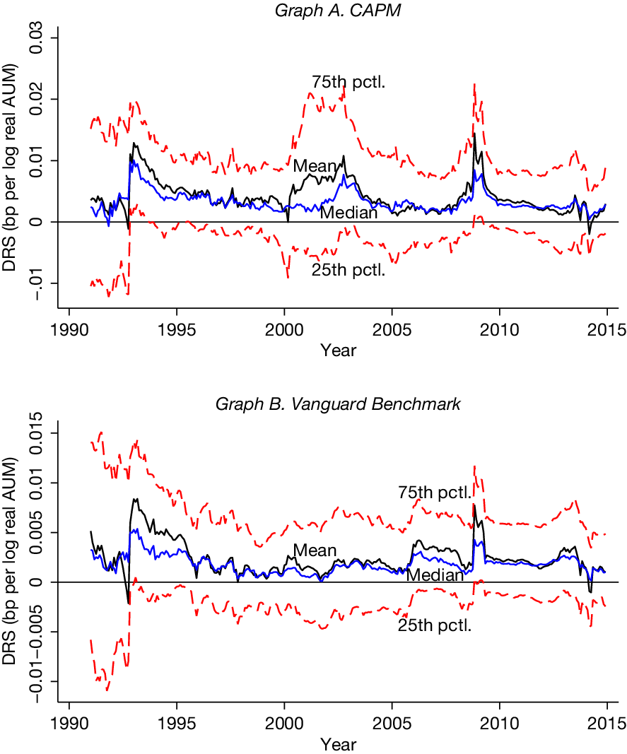

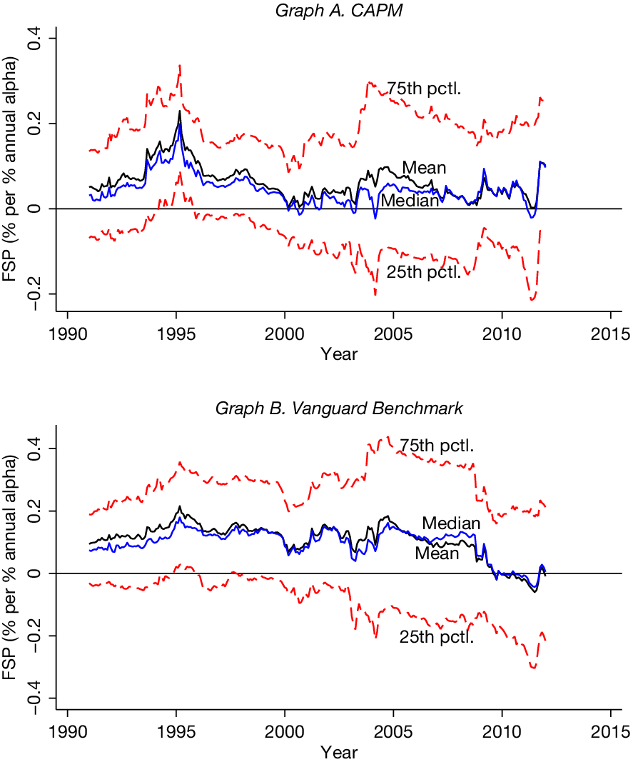

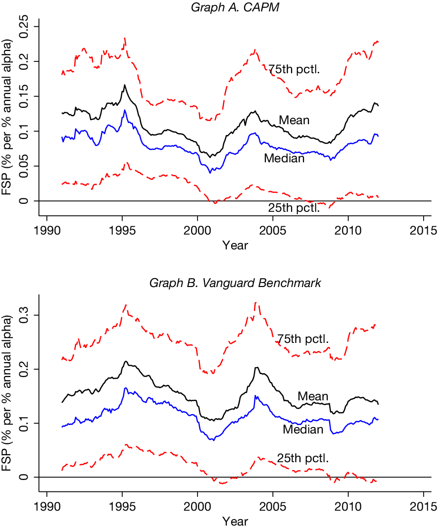

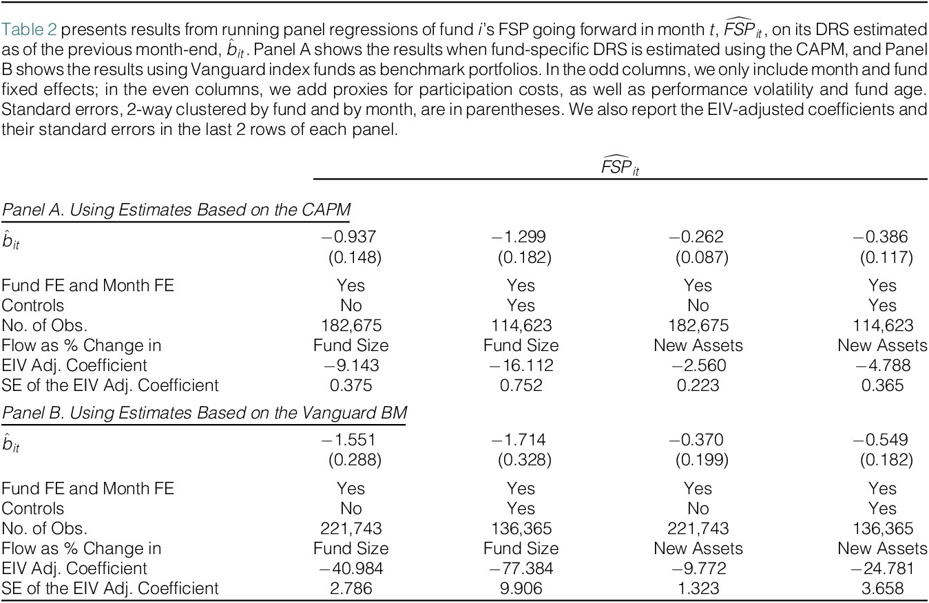


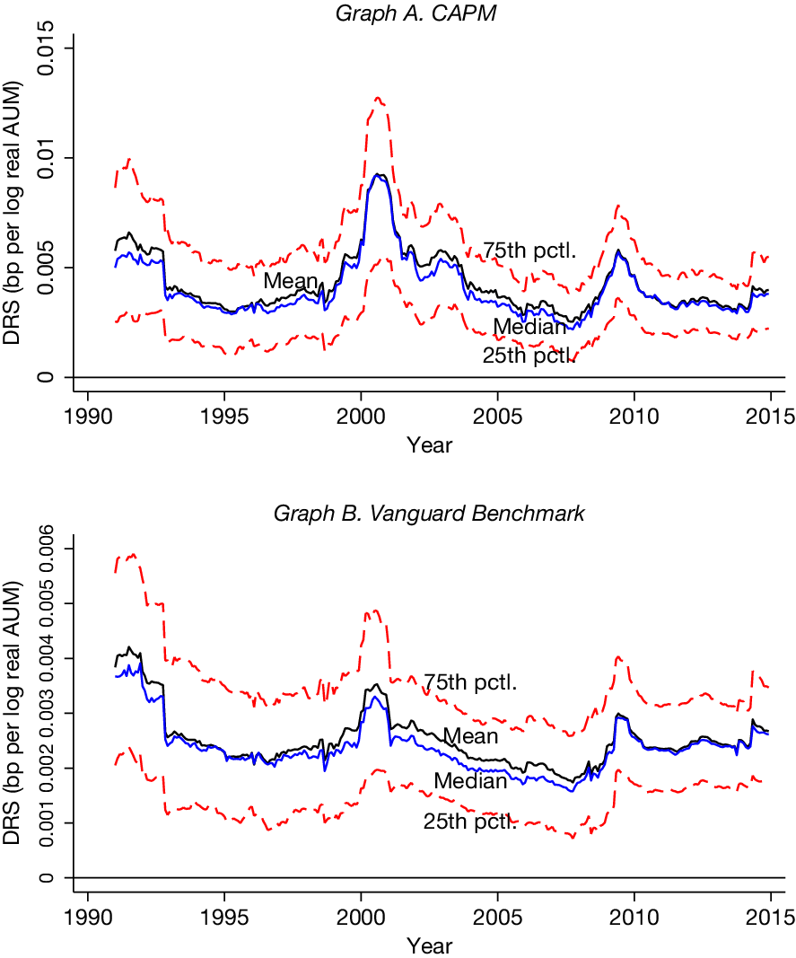

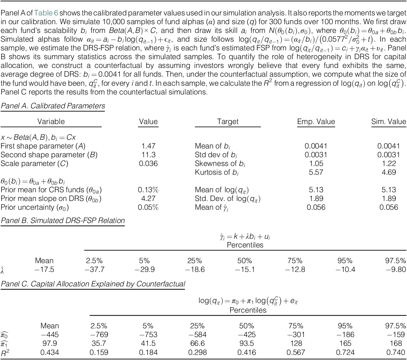
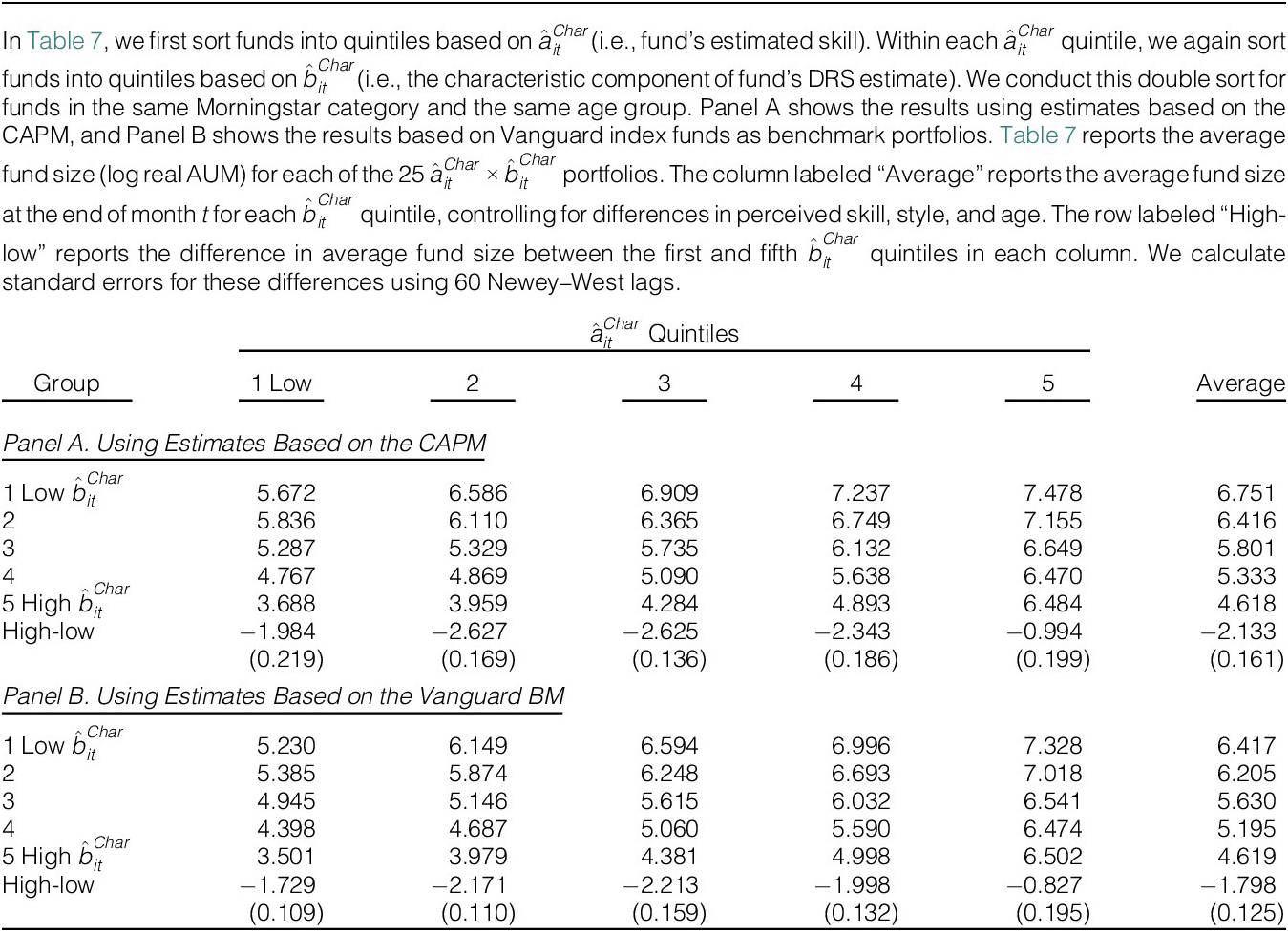


 Open access