A) Partitioning into blocks

H.264/AVC belongs to the category of block-based hybrid video compression schemes. That means that a coded picture, as it is called in the standard, is not encoded in a whole but split into smaller structures that are then encoded separately. Please note that since we do not consider interlacing, we will use the terms coded picture and frame interchangeably. The structures defined by the standard are illustrated in Fig. 2.

Fig. 2. Structures defined by the H.264/AVC standard. A frame consists of disjoint macroblocks that have a size of 16×16 pixels. Several macroblocks can be grouped to disjoint slices. A macroblock can be divided into four sub-macroblocks with a size of 8×8 pixels. Macroblocks and sub-macroblocks can be partitioned into rectangles or squares for motion compensation.

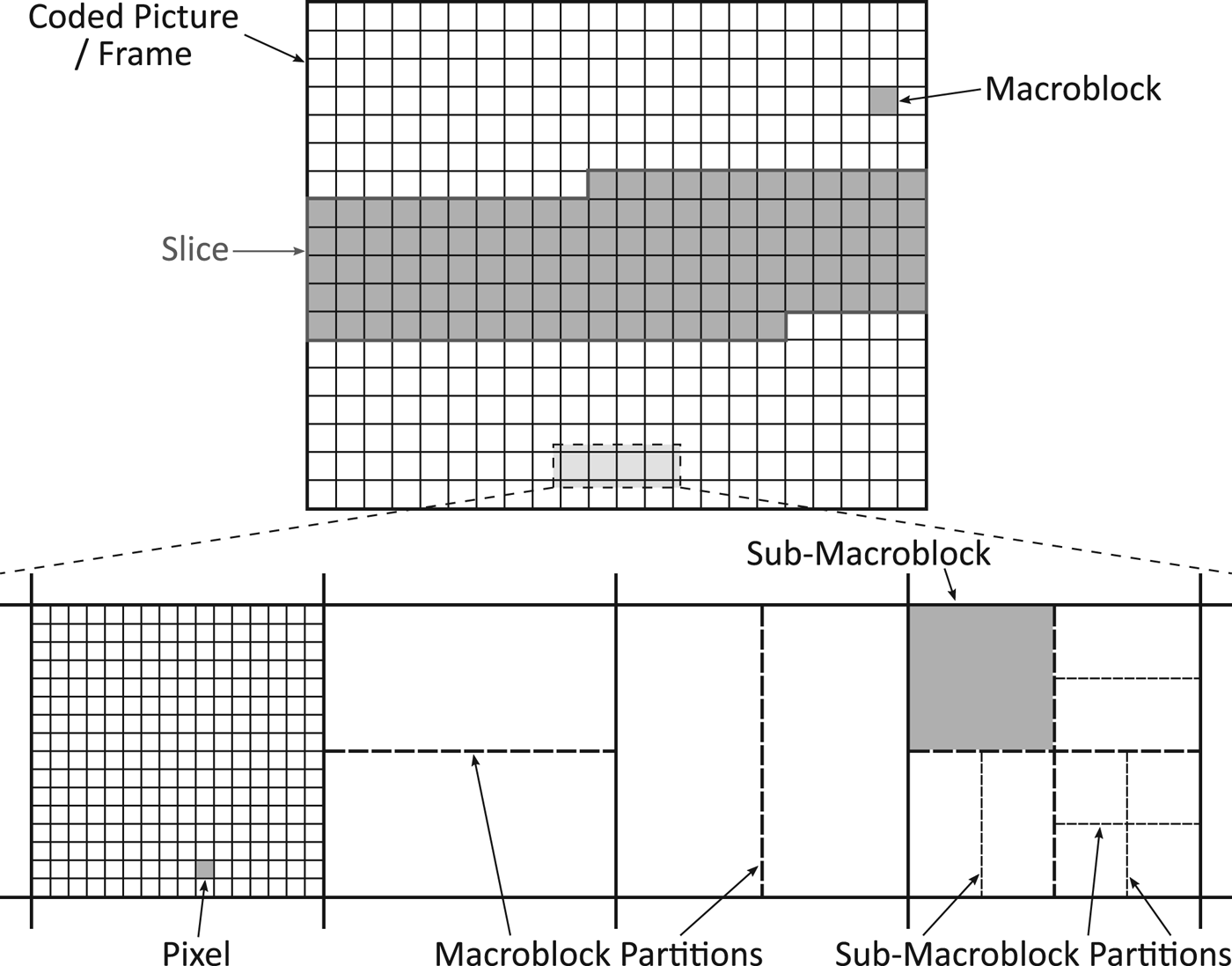
Each frame of a video sequence is divided into so-called macroblocks that have a size of 16×16 pixels. Thereby, the macroblocks are disjoint and arranged in a grid, as can be seen in the upper part of Fig. 2. Furthermore, H.264/AVC defines so-called slices, which are formed by grouping several macroblocks. Slices are also disjoint, i.e., a certain macroblock only belongs to exactly one slice. In the example in Fig. 2, the three slices consist of macroblocks that are connected.

The lower part of Fig. 2 shows how macroblocks are divided into sub-macroblocks and how the blocks can be partitioned for motion compensation, which is used for inter-frame prediction. A macroblock can either not be further divided or be partitioned into two 16×8 blocks, two 8×16 blocks, or four 8×8 blocks. In the case partitioning to 8×8 blocks is selected, these smaller blocks are called sub-macroblocks, which can then also be further partitioned according to the same patterns defined for macroblocks. As a result, the smallest available blocks have a size of 4×4 pixels.

Each macroblock gets assigned a macroblock type that corresponds to the selected partitioning mode. This type is directly extractable from a compressed bit stream, the corresponding syntax element is called mb_type. In the case a macroblock is split into sub-macroblocks, additional syntax elements are added to the bit stream. The element sub_mb_type represents the sub-macroblock type and indicates, similar to mb_type, how this block has been partitioned and predicted.

B) Intra- and inter-frame prediction

As already mentioned, blocks are predicted and only the residual is encoded. There are several methods and modes for the prediction process and not all modes are permitted at any constellation. Similar to mb_type and sub_mb_type, such a type element also exists for slices. The syntax element slice_type defines which macroblock types are permitted within the current slice. Please note that SI and SP slices are not considered here, because they are very rarely used in practice.

If slice_type indicates a so-called I slice, only intra-frame predicted macroblocks, or rather I macroblocks, are allowed. I macroblocks are thereby either directly predicted or split into 4×4 blocks for predicting these partitions separately. The two slice types P and B indicate that inter-frame predicted, or rather P and B macroblocks, are also permitted, in addition to the aforementioned I macroblocks. Furthermore, these slice types permit the encoder to split macroblocks into sub-macroblocks. So, it is possible that a P macroblock has up to 16 motion vectors, in the case all sub-macroblocks have been partitioned into 4×4 blocks. The concept for B macroblocks is similar to that for P macroblocks. The only difference is that these blocks are bidirectionally predicted. Bidirectional prediction further allows another 16 motion vectors per macroblock. Hence, B macroblocks may have up to 32 motion vectors.

The created motion vectors for inter-frame predicted blocks have to be transmitted to the decoder, together with the corresponding frame indices. The frame indices for each block are directly available within the bit stream. Depending on the used list of reference frames, which are called list 0 and list 1, the related syntax elements are ref_idx_l0 and ref_idx_l1, respectively. The motion vectors are not directly included in the bit stream, they are also predicted first. Thereby, the predictor creation is based on already determined neighboring motion vectors. The difference between the actual motion vector and the predictor is then included in the bit stream. The corresponding syntax elements are mvd_l0 and mvd_l1, depending on the used list of reference frames.

C) Transform and quantization

The residuals resulting from intra- or inter-frame prediction are not transferred directly but further processed first. Initially, the residuals are transformed to the frequency domain by a separable integer transform, which has been designed with similar properties as the well-known Discrete Cosine Transform (DCT). The following, important step is the quantization of the transform coefficients. Thereby, a linear quantizer is applied that is controlled by a so-called QP. It can take values from 0 to 51, at which an increasing value yields to increasing quantization step sizes, i.e., a stronger quantization.

The transform and hence the quantization is applied to 4×4 blocks, but the QP is not necessarily the same for all blocks. H.264/AVC defines some metadata structures that are valid for several components. For instance, the Picture Parameter Set (PPS) sets common parameters for several frames. One of these parameters is the initial QP value, which is indicated by the syntax element pic_init_qp_minus26. This QP value is used to quantize all blocks, unless further adaptation is signaled in the bit stream.

For adapting the initial QP value, H.264/AVC defines two additional syntax elements. The first element is slice_qp_delta, which is included in every slice header. If this element is unequal to 0, at this stage, the adapted QP value is valid for all blocks within this slice. However, the finally used QP value can be further changed on macroblock level. The syntax element mb_qp_delta, if included in the bit stream, is used to change the QP value for all blocks within this macroblock.

A) Coordinates and vectors

Before we describe the actual algorithm and its modes, we need to define how to address certain blocks. Thereto, we first define a Cartesian coordinate system, whose point of origin lies at the upper left corner of the first frame of the sequence, in display order. To be more precise, the point of origin is equal to the coordinates of the first 4×4 block of the first frame, which also means that the basis for the system is in 4×4 block precision. Within one frame, blocks are first counted from left to right, and then the rows of blocks are counted from top to bottom.

To address a single block, we either use two-dimensional (2D) or three-dimensional (3D) vectors, depending on the mode in which the algorithm is operating. When using 3D vectors, they are defined by

$${\bf x}^{\rm 3D} := (k,x_1,x_2) \in {\open N}^{3},$$

where ${\open N}$ includes 0. Thereby, k indicates the current frame and hence the temporal direction. As already mentioned, k=0 means the first frame of a sequence in display order. The coordinates x ₁ and x ₂ indicate the block position within the image plane of frame k. For instance, vector (k, 0, 0) describes the position of the first 4×4 block in frame k.

The 2D case defines similar vectors for the image planes. The difference is that the first coordinate k is separated from the vector and used beside it. Hence, the frames are still addressed with k but the vector x is now defined by a 2D vector as

$${\bf x}^{\rm 2D} := (x_1,x_2) \in {\open N}^2.$$

Beside the vectors ${\bf x}^{\rm 2D}$ and ${\bf x}^{\rm 3D}$ , which indicate absolute positions, we need to define displacement vectors. They are basically defined analogously, but their coordinates can take negative values as well. As a consequence, displacement vectors are defined by

$${\bf y}^{\rm 2D} := (y_1,y_2) \in {\open Z}^2$$

and

$${\bf y}^{\rm 3D} := (j,y_1,y_2) \in {\open Z}^3.$$

Furthermore, arithmetic operations on displacement vectors are required to establish the algorithm. Thereto, the 2D and 3D Euclidean norms are defined as usual by

$$\vert {\bf y}^{\rm 2D}\vert := \sqrt{{y_1}^2 + {y_2}^2}$$

and

$$\vert {\bf y}^{\rm 3D}\vert := \sqrt{j^2 + {y_1}^2 + {y_2}^2},$$

respectively.

B) Initial block weighting

The first step in our moving object detection algorithm is assigning a specific weight to each 4×4 block of an incoming frame. These weights reflect the assumed probability of motion within such a block. For determining the weight that should be assigned to a certain block, we analyze the type of the macroblock to which this block belongs to and the used partition mode in case of a P or B macroblock. The reason for this procedure is that the encoder already had to analyze the actual image content to be able to select the most efficient block types and modes. Hence, it is possible to estimate the amount of motion within a block when evaluating the corresponding macroblock type and partition mode.

Since H.264/AVC defines 32 different macroblock types and additionally four sub-macroblock types for the BP and even 58 macroblock and 17 sub-macroblock types for the HP, we group similar types in certain categories at first. Thereby, the categories differ in prediction modes and partition sizes of the contained blocks. An overview of the defined categories is given in Table 1. This table also states the defined initial weights w _init for each category. They have been chosen to express the assumed probability of motion for the specific category. In general, the weight increases with the assumed probability of motion.

Table 1. Categories and initial weights w _init defined according to block types and partition modes of H.264/AVC. All weights depend on a base weight w _base.

All weights depend on a base weight w _base, which defines the weight for the categories with lowest assumed motion. Those are the categories P_SKIP and B_SKIP, i.e., P or B macroblocks that have assigned the special macroblock type SKIP. SKIP mode means that beside the indication for the mode no further information is transmitted for such an inter-frame predicted block, i.e., no residual, no motion vector, and no reference frame index. Instead, the predictor of the block is directly used to reconstruct its content.

Furthermore, the assumption for inter-frame predicted macroblocks is that the finer the partitioning is the higher should be the assumed probability of motion. Hence, the weight for not further divided macroblocks (16×16) is two times the base weight, up to six times the base weight for 4×4 blocks, as can be seen in Table 1. Blocks within intra-frame predicted macroblocks, which are indicated by I_ALL in Table 1, get always assigned the maximum weight of six times the base weight. The reason is that the encoder usually only selects I macroblocks when the block could not predicted with less costly modes, which is valid for blocks containing content that has no counterpart in neighboring frames. This means that this content usually appears the first time in the scene or that an occluded region is visible again. In both cases, this region is to be considered as moving.

It is obvious that this categorization is only valid for P and B slices, since I slices only consist of I macroblocks. Hence, our algorithm just processes inter-frame predicted slices and I slices or frames are interpolated from the results of neighboring frames.

After performing the initial block weighting for a frame, we obtain a map that roughly indicates the probability of containing moving objects for each 4×4 block. Since these maps do not yet enable the extraction of clearly separable regions with moving objects, further processing is required. Hence, the initial weight maps are the input for the algorithm described in the next section.

C) Spatial, temporal, and spatiotemporal weighting

The main part of our algorithm is another weighting step that processes the initial weight maps that have been created as described in the previous section. Thereby, the algorithm is able to operate in two different modes, which can be selected by the user.

In the first mode, a predefined number of frames, including the current frame, is processed in three dimensions in a single step. Thereto, the 3D vectors described in the previous section are used to address single 4×4 blocks. Since neighboring blocks in the spatial and temporal direction are analyzed at the same time, this method can be seen as a spatiotemporal weighting process.

The second mode separates the temporal weighting from the spatial weighting. That means that in a first step incoming frames are spatially processed by weighting the initial weights of the blocks, which are addressed by using the 2D vectors introduced in the previous section. The results of a selected set of frames are then temporally processed by another weighting operation. The benefit of this separation is that a couple of calculations can be omitted and that yields to a significant gain in processing speed.

The two modes are described in detail in the following subsections.

Single-step mode

The single-step mode of our algorithm analyzes several 4×4 blocks of several frames in one equation. To calculate the final weight of a block that indicates the probability of motion within this block, we analyze the initial weights of a certain number of neighboring blocks within the same frame and the same number of blocks in neighboring frames. So, the final weight $w({\bf x}^{\rm 3D})$ of a block at position ${\bf x}^{\rm 3D}$ is calculated by

(1) $$\eqalign{w \lpar {\bf x}^{\rm 3D} \rpar = w_{{\rm init}} \lpar {\bf x}^{\rm 3D} \rpar + {1 \over d_1} \cdot \sum_{{\bf y}^{\rm 3D} \in M^{\rm 3D}} {w_{{\rm init}}\lpar {\bf x}^{\rm 3D} + {\bf y}^{\rm 3D}\rpar \over \Vert {\bf y}^{\rm 3D}\Vert },}$$

where d ₁>0 is a positive constant and set M ^3D is defined by

(2) $$M^{\rm 3D} := \left\{{\bf y}^{\rm 3D} \vert \lpar {\bf y}^{\rm 3D} \neq \lpar 0,0,0 \rpar \rpar \wedge \vphantom{\left({y_2 \over b} \right)^2}\right.$$

(3) $$\quad \lpar -n_{\rm p} \leq j\leq n_{\rm s} \rpar \wedge$$

(4) $$\quad \left. \left(\left({y_1 \over a} \right)^2 + \left({y_2 \over b} \right)^2 \leq 1\right) \right\}$$

where a, b>0 and $n_{\rm p}, n_{{\rm s}}\in {\open N}$ are constant values.

The first summand in (1) represents the initial weight of the current block itself, which hence directly influences the final weight. The second term in (1) is a sum of initial weights of spatially and temporally neighboring blocks that are again weighted with their Euclidean distance to the current block. The influence of this distance can additionally be adapted by parameter d ₁. In general, it is essential that the smaller the distance of the neighboring block to the current block is, the higher is the influence of its initial weight.

The number and positions of the blocks that are considered during the calculation are defined by the set M ^3D. Since the current block itself is already considered by the first term in (1), the displacement vector ${\bf y}^{\rm 3D}$ may not be equal to (0, 0, 0), as indicated by (2). The constant values n _p and n _s in (3) stand for the number of considered preceding and subsequent frames to the current frame, respectively. That means that only blocks whose position's first coordinate j lies within the range of indicated frames are considered. Thereby, j ≡ 0 is valid and indicates the frame the current block belongs to.

The last condition for set M ^3D in (4) defines a region surrounding the current block. According to this definition, the region is 2D with an elliptic shape, whose size is given by the constant values a and b. The center of this ellipse is the current block and all neighboring blocks whose center point lies within this ellipse are considered during the calculation. This is not only valid for the current frame but for all neighboring frames as well. For those, the ellipse is virtually moved to the co-located position within the neighboring frame, i.e., the center point of the ellipse lies on the block with the same Cartesian coordinates x ₁ and x ₂ as for the current block.

Geometrically interpreted the whole region across all considered frames looks like a hose with elliptic profile. This is illustrated in Fig. 3. The current block at a position (k, x ₁, x ₂) for which the final weight should be calculated is marked in dark gray. In this example, n _p=1 and n _s=1, so that three frames are evaluated in total: k−1, k, and k+1. The blocks marked in light gray result from the size and shape of the ellipse, whose semi-axes have been set to a=3.5 and b=2.5 in this example. The ellipse is virtually displaced from frame k to the neighboring frames to determine the blocks to be considered. During the actual calculation all initial weights w _init of considered blocks, which are indicated by the numbers in Fig. 3, are weighted by their Euclidean distance to the current block.

Fig. 3. Illustration of the weighting process. The current block is marked in dark gray and all blocks considered during the calculation are marked in light gray. Numbers within blocks indicate initial weights w _init. Constant values: n _p=n _s=1, a=3.5, b=2.5, and w _base=1.

Two-step mode

The two-step mode is actually very similar to the single-step mode. The only but important difference is that the initial weights are not weighted according to their Euclidean distance in a 3D space but the weighting process takes place in two separate steps. The first step is to calculate an intermediate sum of initial weights for all considered blocks in each involved frame. The considered blocks are thereby all blocks within the defined ellipse, which is still virtually displaced to neighboring frames, but now the sums are determined for each frame separately. This means for the example in Fig. 3 that the three ellipse are individually processed at first.

This sum of initial weights $w_{\rm sum} \lpar k, {\bf x}^{\rm 2D} \rpar $ of a block at position ${\bf x}^{\rm 2D}$ within frame k is mathematically defined by

(5) $$\eqalign{w_{\rm sum} \lpar k, {\bf x}^{\rm 2D} \rpar &= w_{\rm init} \lpar k, {\bf x}^{\rm 2D} \rpar \cr &\quad + {1 \over d_1} \cdot \sum_{{\bf y}^{\rm 2D} \in M^{\rm 2D}} {w_{\rm init} \lpar k, {\bf x}^{\rm 2D} + {\bf y}^{\rm 2D} \rpar \over \vert {\bf y}^{\rm 2D} \vert},}$$

where d ₁>0 is a positive constant. The set M ^2D is defined by

(6) $$M^{\rm 2D} := \left\{{\bf y}^{\rm 2D} \vert \lpar {\bf y}^{\rm 2D} \neq \lpar 0, 0\rpar \rpar \wedge \phantom{\left({y_1 \over a} \right)^2} \right.$$

(7) $$\left. \left(\left({y_1 \over a} \right)^2 + \left({y_2 \over b}\right)^2 \leq 1 \right) \right\}$$

where a>0 and b>0 are positive constants.

In the two-step mode, the initial weights are hence weighted with the 2D Euclidean distance from the corresponding block to the current block. Thereby, the influence of the distance can be adjusted by the parameter d ₁. The set M ^2D is defined analogously to set M ^3D, though the conditions for the temporal direction have been removed.

The second step involves the temporal direction in the calculation. Thereto, the final weight $w(k,{\bf x}^{\rm 2D})$ of a block at position ${\bf x}^{\rm 2D}$ within frame k is calculated by

(8) $$\eqalign{w \lpar k,{\bf x}^{\rm 2D} \rpar & = w_{\rm sum} \lpar k,{\bf x}^{\rm 2D} \rpar \cr &\quad + {1 \over d_2} \cdot \sum_{{j = - n_{\rm p}}\atop{j\neq 0}}^{n_{\rm s}} {w_{\rm sum} \lpar k + j, {\bf x}^{\rm 2D} \rpar \over \vert j \vert },}$$

where d ₂>0 and $n_{\rm p}, n_{\rm s} \in {\open N}$ are positive constants.

The number of neighboring frames is again given according to the parameters n _p and n _s. This time the sums of initial weights are summed up and thereby the value is weighted by the distance |j| between the corresponding frame and the current frame. The parameter d ₂ can be used to adjust the influence of this distance.

The main benefit of the separation of the spatial and temporal weighting process is that several calculations can be omitted. For instance, the sums of initial weights are pre-calculated and can be reused. The single-step mode requires to calculate the weights for each Euclidean distance in each iteration separately. On the other hand, the distance of a block to the current block is determined less accurately than in single-step mode. These pros and cons will also be reflected in the results presented in Section V.

D) Post-processing and segmentation

After creating the final weight maps according to either the single-step or the two-step mode, we additionally apply a 2D discrete N×N Gaussian filter. Thereby, we adopt the filter from our previous work described in [Reference Laumer, Amon, Hutter and Kaup21]. The width N of this filter depends on the standard deviation σ>0 as follows:

(9) $$N = 2 \cdot \left\lceil {6\cdot\sigma + 1\over 2} \right\rceil - 1,$$

where $\lceil \cdot \rceil$ indicates the ceiling function.

It is possible in some cases that there are high differences between the final weights of neighboring blocks and this could result in a patchy segmentation after the final thresholding process. The purpose of the filtering is to smoothen the maps before the actual segmentation.

The only hard decision within our algorithm is the final thresholding process to obtain the segmented binary images. A block at position ${\bf x}^{\rm 2D}$ within frame k is labeled foreground if the following equation becomes true, otherwise the block belongs to the background:

(10) $$w \lpar k, {\bf x}^{\rm 2D} \rpar \geq t \lpar k, {\bf x}^{\rm 2D} \rpar$$

with

(11) $$t\lpar k, {\bf x}^{\rm 2D} \rpar = c_1 \cdot t_{\rm base} - c_2 \cdot {QP}_{\Delta} \lpar k, {\bf x}^{\rm 2D} \rpar ,$$

where c ₁≥1 and c ₂≥0 are constant values.

For the 3D case $w({\bf x}^{\rm 3D})$ is analogously defined by

(12) $$w \lpar {\bf x}^{\rm 3D} \rpar \geq t \lpar {\bf x}^{\rm 3D} \rpar$$

with

(13) $$t \lpar {\bf x}^{\rm 3D} \rpar = c_1 \cdot t_{\rm base} - c_2 \cdot {QP}_{\Delta} \lpar {\bf x}^{\rm 3D} \rpar .$$

In both cases, the base threshold t _base is defined by

(14) $$t_{\rm base} = \lpar \pi \cdot a \cdot b \cdot \lpar n_{\rm p} + n_{\rm s} + 1 \rpar \rpar \cdot w_{\rm base}.$$

Thereby, t _base represents the minimum threshold valid for ellipses in which all blocks have initial weights of w _base. This base threshold can be adjusted by the parameter c ₁.

The second term in (11) and (13) depends on the QP of the corresponding block. In fact, QP _Δ represents the delta between the slice QP and the QP of the corresponding block. That means in cases were the QP has been adjusted on macroblock level, the threshold for these blocks is adjusted, too. As a result of the final thresholding process, each frame is segmented to foreground and background with an accuracy of 4×4 pixels.

A) Performance measures

Before the results of the algorithm can be measured, it is necessary to define a meaningful measurement system. To be comparable and by the reason of using measures everyone is familiar with, the performance of our algorithm is measured by using precision, recall, F score, and receiver operating characteristic (ROC) curves. For the sake of convenience, the measures are briefly described in the following. A more detailed description and a good discussion of the relationship between precision and recall and ROC curves can be found in [Reference Davis and Goadrich25].

Precision and recall compare true positives (TP) with false positives (FP) or false negatives (FN), respectively. So, precision Pr is defined by

(15) $${Pr} = {TP \over TP + FP},$$

and recall Re is defined by

(16) $$Re = {TP \over TP + FN}.$$

That roughly means for detecting an object that recall indicates how much of the object could be detected and that precision indicates how accurate this detection thereby was.

The F score is related or more precisely based on precision and recall. It has been introduced to get a single measure for the performance of an algorithm that can be compared easier. The general F score F _β is defined by

(17) $$F_{\beta} = \lpar 1 + \beta^2 \rpar \cdot {Pr \cdot Re \over \beta^2 \cdot Pr + Re},$$

where β>0 is a factor for weighting either recall higher than precision or vice versa. Since our compressed domain algorithm is intended for being used as a pre-processing step, high recall values are more important than a good precision. Therefore, we provide the F ₂ score that weights recall higher than precision.

Finally, we use ROC curves for determining the optimum parameters. A ROC diagram plots the true positive rate (TPR) against the false positive rate (FPR) of a system at varying settings. The TPR is thereby equally defined as recall by

(18) $$TPR = {TP \over TP + FN}.$$

The FPR is defined by

(19) $$FPR = {FP \over FP + TN},$$

where TN indicates true negatives.

How true/false positives/negatives are counted is a matter of definition. In our case, we simply count pixels by comparing them to manually labeled ground truth in pixel accuracy. This, however, is not advantageous for measuring the performance of our algorithm, since the resulting binary images are in 4×4 pixel accuracy. Comparing these results to ground truth in pixel accuracy will always show a lower precision than comparing them to ground truth that has 4×4 pixel accuracy as well. But to provide a fair comparison with other algorithms, all measures are always based on pixel accuracy in this work.

B) Test setup

We used two different datasets for our experimental tests. The first dataset is the Multi-camera Pedestrian Videos dataset, which has been created by the CVLAB from the EPFL [Reference Berclaz, Fleuret, Türetken and Fua26] and we therefore denote as CVLAB dataset. It contains different scenarios in which the scenes have been captured with several cameras. Since our algorithm is intended for being used in single-view scenarios, we created pixel-wise ground truth for six independent sequences from this dataset: campus4-c0, campus7-c1, laboratory4p-c0, laboratory6p-c1, terrace1-c0, and terrace2-c1. Thereby, the ground truth is available for every tenth frame of the first 1000 frames, respectively.

The second dataset is the Pedestrian Detection Dataset from changedetection.net [Reference Wang, Jodoin, Porikli, Konrad, Benezeth and Ishwar27], which we denote as CDNET dataset. It is a subset of their Dataset2014 dataset and contains ten different sequences: backdoor, busStation, copyMachine, cubicle, office, pedestrians, peopleInShade, PETS2006, skating, and sofa. They provide manually labeled pixel-wise ground truth for each sequence. However, they define temporal regions of interest (ROI) for the sequences, i.e., the ground truth is only available for a subset of frames, respectively. Furthermore, for sequence backdoor there is additionally defined a spatial ROI, i.e., only pedestrians inside of this ROI should be detected. The spatial and temporal ROI are also considered in our evaluation.

All test sequences have been encoded with FFmpeg 2.7.4 (libavcodec 56.41.100) [28] by using the included libx264 [29] library. Thereby, mainly default parameters have been used, except for the following parameters:

• – Profile: Baseline (BP), High (HP)

• – Level: 4.0

• – Group of Pictures (GOP) size: 50

• – Quantization Parameter (QP): 15, 20, 25, 30, 35

As a result, all 16 test sequences have been encoded with ten different configurations and therefore our test set contains 160 sequences.

C) Parameter optimization

As described in Section IV, our algorithm has several adjustable parameters. For finding optimized parameters for the given scenarios, we adopt the procedure described in our previous work in [Reference Laumer, Amon, Hutter and Kaup21]. There we used the c0 sequences from the CVLAB dataset and created 1944 test cases for each sequence. Only one parameter changed from test case to test case, which therefore covered all possible parameter combinations. The optimized parameters, as resulted from this analysis, have been the following: $w_{\rm base} = 1.0$ , d ₁=1.0, d ₂=1.0, a=2.5, b=2.5, n _p=2, n _s=2, σ=1.0, c ₁=1.0, and c ₂=1.0.

In this work, we repeat a part of this analysis. Thereby, we are changing the values of three parameters: σ∈{ off, 1.0, 2.0}, c ₁∈ {1.0, 1.5, 2.0}, and c ₂∈ {0.0, 1.0, 2.0}. All other parameters are fixed and set to the values mentioned above. As a difference to the previous procedure, we test all CVLAB sequences, including both profiles and all QP values, respectively. Furthermore, we test the single-step and the two-step modes. This results in 27 test cases for each sequence-profile-QP-mode combination and hence in 540 test cases for a single sequence.

Figure 4 shows ROC curves for some of the results of this analysis. Since each curve is composed of only 27 supporting points, they appear not very smooth. However, the figures show that our algorithm is able to achieve a high TPR while keeping the FPR low. The upper diagrams 4(a) and 4(b) show ROC curves of all CVLAB sequences tested with single-step and two-step mode, respectively. For the sake of clarity, only the results of the sequences encoded with QP=30 are shown. It can be seen that high TPR are achieved for all sequences. The only exception is sequence campus4-c0, in which several persons stop moving for several frames. Since these persons are then labeled as background, the TPR/recall drops for these frames. The lower diagrams 4(c) and 4(d) depict the results for sequence campus7-c1, including all encoder configurations. What stands out is that the algorithm basically works for every configuration, only low QP values let the FPR increase. This observation is discussed in the next subsection in detail.

Fig. 4. ROC curves of CVLAB test sequences. (BP: Baseline profile; HP: High profile; QP: quantization parameter). (a) CVLAB, single-step mode, QP 30. (b) CVLAB, two-step mode, QP 30. (c) campus7-c1, single-step mode. (d) campus7-c1, two-step mode.

The main result of this analysis is that the previously determined parameter values are already a good choice. Just the standard deviation of the Gaussian filter should be changed to σ=2.0 to obtain the optimum performance. For the sake of completeness, all possible parameter values are again depicted in Table 2. The finally selected parameter values are bold-faced.

Table 2. Adjustable parameters and their possible values. Finally selected values are bold-faced. Source: [Reference Laumer, Amon, Hutter and Kaup21].

D) Results and discussion

Overview

For the determination of the detection performance of our algorithm, we rely on the measures precision, recall, and F ₂ score, as already mentioned above. Figures 5 and 6 show all three measures against the respective QP of the current configuration, for CVLAB and CDNET sequences, respectively. Furthermore, Tables 3 and 4 summarize the results for sequences encoded with QP=30, as an example.

Fig. 5. Precision, recall, and F ₂ score against QP for CVLAB test sequences. (BP: Baseline profile; HP: High profile; QP: quantization parameter). (a) Precision, single-step mode. (b) Precision, two-step mode. (c) Recall, single-step mode. (d) Recall, two-step mode. (e) F ₂ score, single-step mode. (f) F ₂ score, two-step mode.

Fig. 6. Precision, recall, and F ₂ score against QP for CDNET test sequences. (BP: Baseline profile; HP: High profile; QP: quantization parameter). (a) Precision, single-step mode. (b) Precision, two-step mode. (c) Recall, single-step mode. (d) Recall, two-step mode. (e) F ₂ score, single-step mode. (f) F ₂ score, two-step mode.

Table 3. Summary of detection results for CVLAB test sequences encoded with QP=30. Shown are the results of our algorithm in single- and two-step modes, respectively, and the results of the OpenCV [Reference Bradski30] algorithms MOG and MOG2. The first column also indicates the frame size and the number of frames of the respective sequence.

BP, Baseline profile; HP, High profile; Pr, precision; Re, recall; F ₂, F ₂ score; FPS, frames per second.

Table 4. Summary of detection results for CDNET test sequences encoded with QP=30. Shown are the results of our algorithm in single- and two-step modes, respectively, and the results of the OpenCV [Reference Bradski30] algorithms MOG and MOG2. The first column also indicates the frame size and the number of frames of the respective sequence.

BP, baseline profile; HP, High profile; Pr, precision; Re, recall; F ₂, F ₂ score; FPS, frames per second.

The tables additionally provide the results of two pixel-domain object detection algorithms for comparison. Implementations of these two algorithms have been made publicly available by OpenCV 2.4.11 [Reference Bradski30] and are therefore used for comparing our algorithm with the state of the art. Both OpenCV algorithms apply background subtraction methods and rely thereby on modeling the background by using a technique that is called Mixture of Gaussians (MOG). The methods have been proposed by KaewTraKulPong and Bowden [Reference KaewTraKulPong and Bowden31] and by Zivkovic [Reference Zivkovic32] and are called MOG and MOG2 within OpenCV, respectively. We applied both in default configuration; however, the object shadows detected by MOG2 are labeled background in the binary output images.

Figures 5 and 6 again show that our algorithm is able to achieve a high recall. Furthermore, they depict that the performance is highly depending on the stream properties or, more precisely, on the selected QP. Low QP values cause the algorithm to label almost the whole frame as foreground, which indeed results in a recall near 1.0, but the precision drops to almost 0.0. The reason for this is that setting small QP values permits the encoder to spend a large number of bits for each encoded block. As a result, the encoder mainly selects macroblock types with small block partitions or even I macroblocks. Macroblocks in SKIP mode become very rare, which is crucial for our algorithm.

An increasing QP does not only mean an increasing quantization step size, but also that the encoder tries to select low-cost block types wherever applicable. As a consequence, the chosen block types and partition modes reveal more information about the content and therefore promote our algorithm. Having regard to the F ₂ scores, Figs. 5 and 6 show that QP=30 seems to be a good choice with an appropriate trade-off between precision and recall.

Figures 5 and 6, and Tables 3 and 4 as well, additionally allow a comparison between the BP and the HP. For most sequences, using BP or HP does not make a huge difference. However, using the HP almost always achieves a slightly better performance. This effect increases for noisy sequences like laboratory4p-c0 and laboratory6p-c1. Table 3 shows that the precision could be increased from 0.36 to 0.57 or 0.24 to 0.45, respectively. This can be explained by the use of B macroblocks that are more suitable to represent temporal dependencies between frames.

Although using the single-step mode of our algorithm instead of the two-step mode slightly increases the precision as well, this effect is not significant. The reason for this increase is the weighting of, mainly the temporal, neighboring blocks. Since this weighting is performed in a single step and therefore more accurate than in its counterpart, the influence of neighboring blocks is also represented more precisely. The main difference between the single-step and the two-step mode is the processing speed, which is described in Section V.E.

CVLAB sequences

It is obvious that the algorithm's performance depends on the actual video content. Figure 5 shows that the results of some CVLAB sequences differ from the others. Although the precision increases with increasing QP, the advance in precision is less significant for sequences laboratory4p-c0 and laboratory6p-c1. These sequences are noisier than the others and this directly influences the precision negatively. Another example is sequence campus4-c0. The achieved recall for this sequence is significantly lower than for the other sequences. The reason for this is that our algorithm has some difficulties with objects that stop moving. In this case, it is likely that the encoder selects block types that are closer to those of background blocks. So, these blocks would be labeled background although they contain an object. In sequence campus4-c0 three persons are moving around and then one after the other stops, which results in dropping recall values for affected frames.

Figure 7 shows examples of the results of the tested algorithms for sequence campus7-c1. Both the single-step mode and the two-step mode are able to detect the moving person adequately. This results in a recall of 0.92 or even 0.95 for the whole sequence, if encoded with the HP, respectively. Furthermore, our algorithm is able to achieve a high precision by keeping FP low. They mainly only occur near the head or the feet of the person, which is clearly visible in Figs. 7(b) or 7(c), respectively. Hence, the achieved precision for this sequence is 0.74 in single-step mode and 0.71 in two-step mode.

Fig. 7. Sample segmentation of frame 135 of sequence campus7-c1, encoded with HP and QP=30. (Black pixels: TN, green pixels: TP, white pixels: FN, red pixels: FP). (a) Original. (b) Single-step mode. (c) Two-step mode. (d) MOG [31]. (e) MOG2 [32]

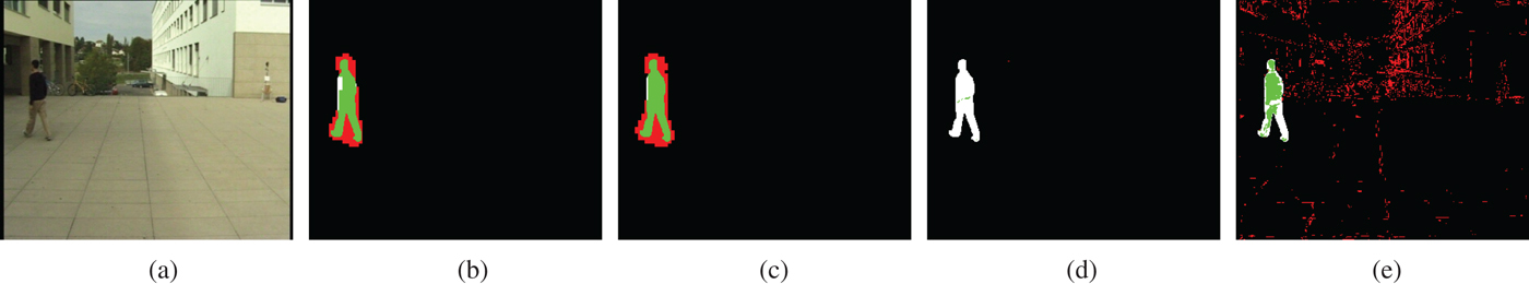
The MOG algorithm seems to have some problems with such sequences. While the precision is always close to or even 1.0, the algorithm is not able to achieve high recall values. This means not only that the background is very well detected, but also that several parts of the moving objects are labeled as background as well. This can be for instance seen in Fig. 7(d). Only a small region in the middle of the person is detected as foreground. One reason is that the background model could not be updated adequately or rather not accurately enough. The pants as well as the pullover of the person have similar color to the background in this image. Hence, the algorithm also labels those foreground parts as background.

The behavior of the MOG2 algorithm is more or less the other way round. Having regard to Fig. 7(e), the person is accurately detected, although there are some missing parts at the legs for the same reason, but the algorithm falsely detects several parts of the background as foreground. As a consequence, the precision drops, in this case only 0.19 could be achieved for the whole sequence.

CDNET sequences

The precision and recall values for CDNET sequences have a higher variance compared with those of CVLAB sequences, as can be seen in Fig. 6. The reason is that these sequences significantly differ in content, mainly in the size and speed of the moving objects. Furthermore, some sequences are more challenging because of difficult scenarios, like for instance standing/stopping or sitting persons (busStation, copyMachine, office, PETS2006, sofa) or abandoned baggage (PETS2006, sofa), which is labeled foreground in the ground truth but obviously not moving and therefore undetectable. Other challenging scenarios that are also included in this dataset are changing camera focus or brightness (copyMachine, peopleInShade), prominent shadows (pedestrians, peopleInShade), and bad weather conditions like snow (skating). Some of those challenging conditions are discussed in the subsequent section.

The sequence backdoor is a good example for sequences from the visual surveillance domain, for which our algorithm is intended for. The scene has a mainly static background and is crossed by moving objects, as can be seen in Fig. 8(a). Furthermore, a spatial ROI is defined, i.e., only the content inside of a certain region is important and everything outside of this region is ignored, which is also frequently used in visual surveillance scenarios. As can be seen in Fig. 6 and also in Table 4, the numerical results for sequence backdoor are very good.

Fig. 8. Sample segmentation of frame 1858 of sequence backdoor, encoded with HP and QP=30. (Black pixels: TN, green pixels: TP, white pixels: FN, red pixels: FP). (a) Original. (b) Single-step mode. (c) Two-step mode. (d) MOG [31]. (e) MOG2 [32].

Visual examples for this sequence for all tested segmentation algorithms are depicted in Fig. 8. Our algorithm is able to detect the persons almost completely, so the respective recall is 1.0 for the two-step mode and 0.99 for the single-step mode. Since FP only occur around the objects themselves, which is mainly because of the lower accuracy of 4×4 pixels or larger, the achieved precision is satisfying as well. When using the two-step mode, the precision is 0.65 and the single-step mode even reaches 0.71.

As before, it seems that MOG and MOG2 have some difficulties in updating their background model at this sequence. While in this example FP almost not occur when using MOG, several parts of the persons are not detected but falsely labeled background. For instance, the pullover of the woman on the right has a color close to the color of the wall in the background. The result is that the pattern of the fence becomes visible in the segmented image, because the pullover is easily distinguishable from the black fence but not from the lighter wall.

The recall achieved by MOG2 is much higher than by MOG, so the persons are detected well. The precision on the other hand is only 0.08 for sequence backdoor. A reason for this can be seen in Fig. 8(e), in which the lighter parts of the ground, i.e., regions without shadows, are falsely detected as foreground. This increases the FP and hence decreases the precision.

Challenging conditions

As already mentioned, the CDNET dataset contains several sequences with challenging conditions. Generally, the most analysis algorithms are challenged by a changing camera focus, automatically adapted brightness, fast moving objects, prominent object shadows, and bad weather conditions. Such scenarios are also included in the CDNET dataset.

Figure 9 shows three sample images from CDNET sequences with their corresponding segmentation of our algorithm in two-step mode. Thereby, Fig. 9(a) illustrates that prominent shadows will be detected by the algorithm as well. This is obvious because the shadows are moving in conjunction with the object itself and it is not possible to distinguish between the object and the shadow at this stage. The creators of the ground truth of the CDNET sequences hence also labeled prominent shadows as foreground in most of the sequences, as can be seen in the lower image of Fig. 9(a).

Fig. 9. Sample segmentation of some sequences with challenging conditions, encoded with HP and QP=30. The upper row shows the original frames, the lower row the results from our algorithm in two-step mode. (Black pixels: TN, green pixels: TP, white pixels: FN, red pixels: FP). (a) peopleInShade, frame 296. (b) pedestrians, frame 474. (c) skating, frame 902.

This is different in Fig. 9(b). The shadow of the cyclist is indeed again detected but it is not labeled as foreground in the ground truth this time. Hence, this region (below the person on the right) is marked red in the lower image of Fig. 9(b). Another observation at this result image is that a relatively large region behind the cyclist in wrongly detected by the algorithm. This occurs when objects are moving very fast compared with the frame rate. In this case, the displacement of the object's position is significant between two consecutive frames. And this results in FP behind the object because of the temporal analysis of several frames.

Finally, a worst case scenario is depicted in Fig. 9(c). As can bee seen, the number of FP is very high in this case. The reason for this is the heavy snowfall in front of the camera. However, these false detections mainly only occur in regions in which the contrast between the white snow and the darker background is high. The lower parts of the persons are generally detected satisfactorily.

In addition to the challenging scenarios mentioned above, Fig. 10 shows a scenario with stopping objects, including an abandoned bag, which is also challenging for our algorithm, since it is intended to detect moving regions within a video sequence. The first segmentation result in Fig. 10(a) shows that all persons are detected as intended due to the fact that they are moving. In the next image in Fig. 10(b), the person in the center of the scene stopped moving, which results in only a partial detection. Some frames later (cf. Fig. 10(c)), the person drops its backpack, which is again detected because the person is moving by doing so. Figure 10(d) again shows that both, the person and the backpack, are not detected by the algorithm when none of them is moving. In this case, in which the persons stands still for several frames, it is obvious that the encoder selected the SKIP mode for encoding the corresponding macroblocks. Finally, it can be seen in Fig. 10(e) that the person is detected again when it starts moving again. Since the backpack is left behind, it is still not detectable.

Fig. 10. Sample segmentation of frames 411, 522, 902, 1050, and 1126 of sequence PETS2006, encoded with HP and QP=30. The upper row shows the original frames, the lower row the results from our algorithm in two-step mode. (Black pixels: TN, green pixels: TP, white pixels: FN, red pixels: FP). (a) Frame 411. (b) Frame 522. (c) Frame 902. (d) Frame 1050. (e) Frame 1126.

All those examples show, even in challenging scenarios, moving objects are detected as intended by our algorithm. In some scenarios, applying the method results in increased FP and hence a decreased precision on pixel level. But in terms of detecting objects, no object is missed, which is the most important task for compressed domain algorithms that are used to preselect certain regions for further analysis. An exception are stopping objects, which are not detectable anymore due to the characteristics of our algorithm. But since such objects will definitely have been detected in the moment they entered the scene, they can also be considered as not missed. Additional segmentation results can also be found in Figs. 11–14.

Fig. 11. Sample segmentation of frame 935 of sequence laboratory4p-c0, encoded with HP and QP=30. (Black pixels: TN, green pixels: TP, white pixels: FN, red pixels: FP). (a) Original. (b) Single-step mode. (c) Two-step mode. (d) MOG [31]. (e) MOG2 [32].

Fig. 12. Sample segmentation of frame 615 of sequence terrace1-c0, encoded with HP and QP=30. (Black pixels: TN, green pixels: TP, white pixels: FN, red pixels: FP). (a) Original. (b) Single-step mode. (c) Two-step mode. (d) MOG [31]. (e) MOG2 [32].

Fig. 13. Sample segmentation of frame 2463 of sequence cubicle, encoded with HP and QP=30. (Black pixels: TN, green pixels: TP, white pixels: FN, red pixels: FP). (a) Original, (b) Single-step mode (c) Two-step mode (d) MOG [31] (e) MOG2 [32].

Fig. 14. Sample segmentation of frame 1051 of sequence busStation, encoded with HP and QP=30. (Black pixels: TN, green pixels: TP, white pixels: FN, red pixels: FP). (a) Original. (b) Single-step mode. (c) Two-step mode. (d) MOG [31]. (e) MOG2 [32].

E) Processing speed

Compressed domain algorithms are known to be less complex than their pixel domain counterparts, mainly for two reasons. First, the costly step of decoding is replaced by simple syntax parsing operations and, second, the algorithms themselves are low-complex because they usually do not have to process all pixels. However, it is not always an easy task to directly compare different algorithms with regard to their processing speeds, especially in cases where these algorithms have been implemented supremely different.

In our implementation, we incorporated the reference implementation of the H.264/AVC standard, the JM software (JM-18.6) [33], for parsing the required syntax elements. Since the purpose of this software is not to be implemented highly optimized, it can be assumed that the decoder used by OpenCV, which is part of FFmpeg, performs much faster. Furthermore, our test implementation of the actual algorithm is also not optimized. So, in some cases, the software loops up to ten times over all 4×4 blocks of a single frame, including initializations and conversions between container formats. The OpenCV implementations, on the other hand, are usually highly optimized towards a low complexity.

Nevertheless, we measured the execution times of all tested algorithms, because we think it is important to provide this information. Tables 3 and 4 provide the processing speeds, in terms of frames per second, for the stated test sequences. Thereby, the time that has been required for parsing the syntax elements as well as the time for the actual algorithm has been measured for our algorithm. Correspondingly, the processing time for MOG and MOG2 includes the decoding and the analysis time. Furthermore, the given values are average values determined by executing each test ten times. The reason for averaging several results is that the processing speeds of MOG and MOG2 are highly fluctuating – the speed of our algorithm is almost not varying when performing the same test several times – and an average is more significant for the comparison. The tests have been performed on a relatively old desktop computer: Intel Core 2 Duo E8400 CPU @ 3.0 GHz, 8 GB DDR2 RAM, Windows 10 Pro 64-Bit. Because of the dual-core architecture, two tests have been performed in parallel.

It can be seen that the algorithm in two-step mode operates much faster than in single-step mode. For instance, the two-step mode is able to analyze about 133 frames per second in average for CVLAB sequences, while the single-step mode only achieves about 40. The reasons for this are the omitted calculations in two-step mode, as already explained in Section IV. Furthermore, it is obvious that the processing speed directly depends on the frame size, since a larger frame size means more blocks to be processed. So, for instance, only 37 frames of sequence PETS2006 could be processed per second.

Although the MOG algorithm is a pixel domain algorithm, it performs very fast. And because of the missing optimizations in our algorithm, it even operates faster than our compressed domain algorithm. The drawback is that our algorithm achieves better detection results for almost all our test sequences. Compared to the MOG2 algorithm, the proposed algorithm in two-step mode always runs just as fast or faster, even without optimizations.

As already mentioned, our algorithm uses the JM software [33] for the syntax parsing. Parsing the 1010 frames of a single CVLAB sequence that has been encoded with ${QP} = 30$ and the HP takes about 3 seconds. Performing our two-step analysis algorithm then takes another 5.2 seconds. This results in about 123 frames per second, as also stated in Table 3. So, above 36% of the overall processing time is required by the JM software to parse the syntax elements. This could be significantly decreased by incorporating a more efficient decoder, or rather parser. The implementation of the actual algorithm is also not optimized but is able to process 1010 frames of a CVLAB sequence in about 5.2 seconds, which results in about 194 frames per second. This could be increased as well by optimizing the test implementation. And even parallel processing is imaginable, for instance, the initial block weighting process for several frames could be performed in parallel, which would increase the processable number of frames even further.