


1. Introduction
Our present concern is with linear global instability mechanisms associated with unsteadiness of laminar three-dimensional separated flows over finite aspect ratio, untapered swept wings at low Reynolds numbers. To date, the vast majority of instability studies have focused on simplified models of laminar separation with no spanwise base flow component, as encountered in flows over two-dimensional profiles, or spanwise homogeneous flow over infinite-span wings, both of which have been used as proxies to understand fundamental mechanisms of separation in practical fixed- or rotary-wing applications. However, either of these approximations fails to address the essential three-dimensionality of the flow field (Wygnanski et al. Reference Wygnanski, Tewes, Kurz, Taubert and Chen2011; Wygnanski, Tewes & Taubert Reference Wygnanski, Tewes and Taubert2014) and the implications of linear instability of three-dimensional separated flow on the ensuing unsteadiness on a finite-span swept wing. Presently there exists limited knowledge on linear instability mechanisms associated with three-dimensional separation on the wing surface, or a deep understanding of the complex vortex dynamics arising from this instability on a finite-span wing, as a function of the aspect ratio  $(AR)$ and angles of attack $(\alpha )$ and sweep $(\varLambda )$. In fact, there is a void in the literature that employs three-dimensional global (TriGlobal) linear instability analysis appropriate for the fully inhomogeneous three-dimensional flow field around a finite $AR$ wing at high $\alpha$. The present work aims to close this knowledge gap by documenting modal instability mechanisms and their evolution on different wing geometries.
A review of existing literature on the subject sets the scene for the work performed herein. Studies of separation have extensively analysed laminar separation bubbles (LSBs) in the context of flat plates. Although such bubbles were known to be structurally unstable (e.g. Dallmann Reference Dallmann1988), Theofilis, Hein & Dallmann (Reference Theofilis, Hein and Dallmann2000) showed that the physical mechanism leading to unsteadiness and three-dimensionalisation of a nominally two-dimensional LSB, as well as to breakdown of the associated vortex, arises from self-excitation of a previously unknown stationary three-dimensional global mode. Soon after that, global linear stability theory was applied to two-dimensional airfoils (Theofilis, Barkley & Sherwin Reference Theofilis, Barkley and Sherwin2002) and unswept wings of infinite span (Kitsios et al. Reference Kitsios, Rodríguez, Theofilis, Ooi and Soria2009). Rodríguez & Theofilis (Reference Rodríguez and Theofilis2010) studied structural changes experienced by the LSB on a flat plate due to the presence of the unstable stationary three-dimensional global mode and established a criterion of approximately  $7.5\,\%$ backflow for self-excitation of the nominally two-dimensional flow. Furthermore, linear superposition of the global mode discovered by Theofilis et al. (Reference Theofilis, Hein and Dallmann2000) upon the two-dimensional LSB revealed the well-known three-dimensional U-separation pattern (Hornung & Perry Reference Hornung and Perry1984; Perry & Chong Reference Perry and Chong1987; Délery Reference Délery2013), whereas the surface streamlines topology induced by the global mode resembled the characteristic cellular structures known as stall cells (SCs) (Moss & Murdin Reference Moss and Murdin1968; Bippes & Turk Reference Bippes and Turk1980; Winkelman & Barlow Reference Winkelman and Barlow1980; Weihs & Katz Reference Weihs and Katz1983; Bippes & Turk Reference Bippes and Turk1984; Broeren & Bragg Reference Broeren and Bragg2001; Schewe Reference Schewe2001), that are observed to form on stalled wings. Finally, Rodríguez & Theofilis (Reference Rodríguez and Theofilis2011) have extended this analysis to a real LSB on an infinite span wing, showing that the surface streamlines generated by the leading global modes strongly resemble SCs.
Massively separated spanwise homogeneous flow over stalled wings was studied by He et al. (Reference He, Gioria, Pérez and Theofilis2017a) using global linear modal and non-modal stability tools. Flow over three different NACA airfoils was analysed at  $150 \leq Re \leq 300$ and $10^\circ \leq \alpha \leq 20^\circ$. A travelling Kelvin–Helmholtz (K–H) mode dominating the flow at a large spanwise periodicity length and a three-dimensional stationary mode most active as the spanwise periodicity length becomes smaller were identified. Non-modal analysis showed that linear optimal perturbations evolve into travelling K–H modes. Secondary instability analysis of the time-periodic base flow ensuing linear amplification of the K–H mode revealed two amplified modes with spanwise wavelengths of approximately 0.6 and 2 chords. These modes are reminiscent of the classic mode A and B instabilities of the circular cylinder (Barkley & Henderson Reference Barkley and Henderson1996; Williamson Reference Williamson1996) although, unlike on the cylinder, the short-wavelength perturbation was the first to become linearly unstable. This work showed that SC-like streamline patterns on the wing arise from linear amplification of this short-wavelength secondary instability. By contrast to the primary instability based scenario proposed by Rodríguez & Theofilis (Reference Rodríguez and Theofilis2011), this mechanism could explain the emergence of SC at lower angles of attack.
Zhang & Samtaney (Reference Zhang and Samtaney2016) extended the analysis of He et al. (Reference He, Gioria, Pérez and Theofilis2017a) to study instability of unsteady flow over a NACA 0012 spanwise periodic wing at higher Reynolds numbers,  $400 \leq Re \leq 1000$ at $\alpha =16^\circ$. At $Re=800$ and 1000 these authors identified two oscillatory unstable modes corresponding to near-wake and far-wake instabilities, alongside a stationary unstable mode, whereas only one unstable mode was found at the lower $Re=400$ and 600. Ground-proximity effects on the stability of separated flow over NACA 4415 at low Reynolds numbers were studied using two-dimensional global (BiGlobal) theory with consideration of both flat (He et al. Reference He, Pérez, Yu and Li2019c) and wavy ground surfaces (He et al. Reference He, Guan, Theofilis and Li2019b). Finally, Rossi et al. (Reference Rossi, Colagrossi, Oger and Le Touzé2018) considered incompressible flow over a NACA 0010 airfoil and a narrow ellipse of the same thickness at a large $\alpha$ of $30^\circ$ ( $100 \leq Re \leq 3000$) documenting multiple bifurcations. The aforementioned efforts have certainly enriched our understanding of instability mechanisms of spanwise homogeneous flow over wings of infinite span. However, BiGlobal analysis cannot be applied to address the instability of fully three-dimensional vortical patterns arising in finite $AR$ wing flows.
Before discussing the application of the appropriate linear TriGlobal modal analysis, a brief review of experimental and numerical work on finite aspect ratio wings is presented. Early experimental studies on finite  $AR$ wings are summarised in Boiko et al. (Reference Boiko, Dovgal, Zanin and Kozlov1996). On three-dimensional swept wings in particular, the presence of significant spanwise flow leads to three-dimensional flow structures such as the ‘ram's horn’ vortex (Black Reference Black1956). As soon as local stall appears on a swept wing, spanwise boundary layer flow alters the stall characteristics of sections with attached flow along the span (Harper & Maki Reference Harper and Maki1964). More recently, aerodynamic performance of small aspect ratio $(AR=0.5\unicode{x2013}2)$ wings has been studied experimentally (Torres & Mueller Reference Torres and Mueller2004) and computationally (Cosyn & Vierendeels Reference Cosyn and Vierendeels2006). Taira & Colonius (Reference Taira and Colonius2009) used three-dimensional direct numerical simulation (DNS) to study impulsively translated flat-plate wings ( $AR=1\unicode{x2013}4$) of different planforms at a wide range of $\alpha$ and $300 \leq Re \leq 500$. The $AR$,
$AR$,  $\alpha$ and Reynolds number were found to have a large influence on the stability of the wake profile and the force experienced by the finite wing with the flow reaching a stable steady state, a periodic cycle or aperiodic shedding. The three-dimensional nature of the flow was highlighted, and tip effects were found to stabilise the flow and exhibit nonlinear interaction with the shedding vortices. Even at larger $AR=4$ the flow did not reach two-dimensional von Kármán vortex shedding due to the emergence of SC-like patterns. The effects of trapezoidal rather than rectangular planform (Huang et al. Reference Huang, Venning, Thompson and Sheridan2015), and larger $AR$ wings (Son & Cetiner Reference Son and Cetiner2017) have been considered in more recent publications.
In the general context of vortex dynamics, a large body of experimental and large-scale numerical simulation work exists on separated flows over finite  $AR$ wings. There are studies analysing complex vortex dynamics under unsteady manoeuvres including translation and rotation (Kim & Gharib Reference Kim and Gharib2010; Jones et al. Reference Jones, Medina, Spooner and Mulleners2016), surging and plunging (Calderon et al. Reference Calderon, Cleaver, Gursul and Wang2014; Mancini et al. Reference Mancini, Manar, Granlund, Ol and Jones2015), pitching (Jantzen et al. Reference Jantzen, Taira, Granlund and Ol2014; Son & Cetiner Reference Son and Cetiner2017; Smith & Jones Reference Smith and Jones2020) and flapping (Dong, Mittal & Najjar Reference Dong, Mittal and Najjar2006; Medina et al. Reference Medina, Eldredge, Kweon and Choi2015). These works focused on the analysis of large-scale flow structures such as leading edge vortices (Gursul, Wang & Vardaki Reference Gursul, Wang and Vardaki2007; Eldredge & Jones Reference Eldredge and Jones2019) which can augment unsteady vortical lift and offer opportunities for flow control (Gursul, Cleaver & Wang Reference Gursul, Cleaver and Wang2014). However, none of these studies have looked at the global instability mechanisms of these flows.
In the framework of linear stability analysis of finite wings, works exist that consider the entire flow field but typically at low  $\alpha$ (that allows the use of streamwise periodicity assumption). He et al. (Reference He, Tendero, Paredes and Theofilis2017b) performed linear global instability analysis using spatial BiGlobal eigenvalue problem and linear PSE-3D disturbance equations in the wake of a low $AR$ three-dimensional wing of elliptic planform constructed using the Eppler E387 airfoil at $Re=1750$. Symmetric perturbations corresponding to the instability of the vortex sheet connecting the trailing vortices and antisymmetric perturbations peaking at the vortex sheet and also in the neighbourhood of the trailing vortex cores were identified. Edstrand et al. (Reference Edstrand, Schmid, Taira and Cattafesta2018a) carried out spatial and temporal stability analysis of a wake and trailing vortex region behind a NACA 0012 finite wing at $Re=1000$, $\alpha =5^{\circ }$ and $AR=1.25$, documenting seven unstable modes with the wake instability dominating in both temporal and spatial analyses. Unlike many stability analysis works focusing only on the vicinity of the tip vortex, the full half-span of the wing was considered. BiGlobal stability analysis was employed exploiting streamwise homogeneity in the absence of large scale separation at the low $\alpha$ considered. This allowed capturing three-dimensional modes with structures in the tip and the wake regions. Subsequent work of Edstrand et al. (Reference Edstrand, Sun, Schmid, Taira and Cattafesta2018b) on the same geometry employed parabolised stability analysis to guide the design of active flow control for tip vortex based on a subdominant instability mode that was found to counter-rotate with the tip vortex. Forcing of this mode introduced at the trailing edge was shown to attenuate the tip vortex. Navrose, Brion & Jacquin (Reference Navrose, Brion and Jacquin2019) conducted TriGlobal non-modal stability analysis of a trailing vortex system over a flat plate and NACA 0012 wing at $\alpha =5^\circ$, $AR=6$ and $Re=1000$. Unlike in earlier studies, their fully three-dimensional analysis included the tip vortex and flow over the wing. It was shown that the linear optimal perturbation is located near the wing surface and advects into the tip vortex region during its evolution, which agrees with the findings of Edstrand et al. (Reference Edstrand, Sun, Schmid, Taira and Cattafesta2018b). The displacement of the vortex core due to evolution of the optimal perturbation was proposed as a possible mechanism behind trailing vortex meandering. All these studies have demonstrated that addressing the three-dimensionality of finite wing wake through stability analysis allows for enhanced understanding of the underlying physical mechanisms. However, the relatively low angles of attack considered in these studies meant that the underlying base flows had a relatively simple vortical structure.
In the framework of our present combined theoretical/numerical and experimental efforts, Zhang et al. (Reference Zhang, Hayostek, Amitay, He, Theofilis and Taira2020b) employed DNS to analyse the development of three-dimensional separated flow over unswept finite wings at a range of  $\alpha$ $({Re=400},\ 1 \leq AR \leq 6)$. The formation of three-dimensional structures in the separated flow was discussed in detail. The vortex sheet from the wing tip rolls up around the free end to form the tip vortex which at first is weak with its effects spatially confined. As the flow around the tip separates, the tip effects extend farther in the spanwise direction, generating three-dimensionality in the wake. It was shown that the tip-vortex-induced downwash keeps the wake stable at low $AR$, whereas at higher $AR$ unsteady vortical flow emerges and vortices are shed forming closed loops. At $AR\gtrsim 4$ tip effects slow down the shedding process near the tip, which desynchronises from the two-dimensional shedding over the midspan region, giving rise to vortex dislocation. The interactions of the tip vortex with the unsteady wake structures at high $\alpha$ lead to noticeable tip vortex undulations. Subsequently, Zhang et al. (Reference Zhang, Hayostek, Amitay, Burtsev, Theofilis and Taira2020a) addressed swept wing flows at the same conditions. Several stabilisation mechanisms additional to those found in Zhang et al. (Reference Zhang, Hayostek, Amitay, He, Theofilis and Taira2020b) were reported for swept wings. At small $AR$ and low $\varLambda$, the tip vortex downwash effects still stabilise the wake, whereas the weakening of the downwash with increasing span allows the formation of unsteady vortex shedding. For higher $\varLambda$, the source of three-dimensionality was shown to transition from the tip of the wing to midspan where a pair of symmetric vortical structures is formed with their mutually induced downward velocity stabilising the wake. Therefore, three-dimensional midspan effects leading to the formation of stationary vortical structures allow steady flow formation at higher $AR$ which would not be feasible on unswept wings. At higher $AR$ the midspan effects weaken near the tip leading to unsteady vortex shedding in the wing tip region. Finally, for high $AR$ and high $\varLambda$ wings, steady flow featuring repetitive formation of the streamwise aligned finger-like vortices along the span ensues.
Despite the substantial improvement in understanding of complex vortical structures that recent computational efforts have offered, several key questions remain open and motivate the present work. First, the origin of the wake unsteadiness observed in the simulations of Zhang et al. (Reference Zhang, Hayostek, Amitay, He, Theofilis and Taira2020b) and those performed herein, remains unexplained and the conjecture that this unsteadiness arises on account of a presently unknown flow eigenmode needs to be examined. Further, the frequency content and spatial structure of this (and possibly other) modes existing in the flow both during the linear regime and at nonlinear saturation needs to be documented and classified. Finally, the effects of wing geometry on the global modes, especially that of  $\varLambda$ and $AR$, needs to be examined. In order to address these questions, we perform linear TriGlobal modal analysis of separated flow over finite three-dimensional wings, followed by a brief data-driven modal analysis (Taira et al. Reference Taira, Brunton, Dawson, Rowley, Colonius, McKeon, Schmidt, Gordeyev, Theofilis and Ukeiley2017) once the leading three-dimensional global mode has led the flow to nonlinear saturation.
Finally, the choice of the flow analysed with respect to its stability deserves some discussion. Stability analysis of the mean flow, obtained by time-averaging the unsteady periodic flow, has been shown to accurately predict the frequency of the unsteadiness in certain types of flows (Barkley Reference Barkley2006; Beneddine et al. Reference Beneddine, Sipp, Arnault, Dandois and Lesshafft2016). This was explained using weakly nonlinear analysis by Sipp & Lebedev (Reference Sipp and Lebedev2007), who formulated two conditions in terms of the complex constants of the Stuart–Landau equation that must hold for linear stability analysis of a mean flow to be relevant. It was demonstrated that these conditions are satisfied for the circular cylinder near the critical Reynolds number considered by Barkley (Reference Barkley2006). A discussion of this point in the context of the present fully three-dimensional flow will be presented in the closing chapters, after the main body of results, obtained using base flows that numerically satisfy the equations of motion, has been presented.
The paper is organised as follows. The theory underlying linear modal stability analysis is discussed in § 2 followed by the explanation of computational set-up and numerical methods as well as verification of stability analysis tools in § 3. Results are reported in § 4 starting with the discussion of the base flow. Linear global modes and the effects of wing geometry at  $Re=400$ and $\alpha =22^\circ$ are reported in § 4.2. The effects of varying Reynolds number and $\alpha$ are considered in § 4.3. Finally, the growth of the leading global mode and eventual transition to nonlinearity is discussed in § 4.4.
2. Theory
The flow under consideration is governed by the non-dimensional, incompressible Navier–Stokes and continuity equations:
 \begin{equation} \partial_t {\boldsymbol u} + {\boldsymbol u} \boldsymbol{\cdot} \boldsymbol{\nabla}{\boldsymbol u} ={-}\boldsymbol{\nabla} p + Re^{{-}1} \nabla^2 \boldsymbol u,\quad \boldsymbol{\nabla} \boldsymbol{\cdot} \boldsymbol u = 0, \end{equation}
where the Reynolds number,  $Re \equiv U_\infty c/\nu$, is defined by reference to the free-stream velocity, $U_\infty$, the chord, $c$, and the kinematic viscosity, $\nu$. The flow field can be expressed on an orthogonal coordinate system as a function of the unsteady velocity $\boldsymbol {u}=(u,v,w)^{\rm T}$ and pressure
 \begin{equation} \boldsymbol{q}(\boldsymbol{x},t) = (u,v,w, p)^{\rm T}, \end{equation}
which are decomposed into a base flow component  $\boldsymbol {\bar {q}}$ and a small perturbation $\boldsymbol {\tilde {q}}$ with unit magnitude, such that
 \begin{equation} \boldsymbol{q} = \boldsymbol{\bar{q}} + \varepsilon \boldsymbol{\tilde{q}},\quad \varepsilon \ll 1. \end{equation}
The approach followed to obtain steady stable, or stationary unstable base flows are discussed in § 3.3. Substituting (2.3) into (2.1a,b), subtracting the base flow at  $O(1)$ and neglecting $O(\varepsilon ^2)$ terms leads to the linearised Navier–Stokes equations (LNSEs)
 \begin{equation} \partial_t {\tilde{\boldsymbol{u}}} + \bar{\boldsymbol{u}} \boldsymbol{\cdot} \boldsymbol{\nabla}{\tilde{\boldsymbol{u}}} + \tilde{\boldsymbol{u}} \boldsymbol{\cdot}\boldsymbol{\nabla}{\bar{\boldsymbol{u}}} ={-}\boldsymbol{\nabla} \tilde{p} + Re^{{-}1} \nabla^2 \tilde{\boldsymbol{u}},\quad \boldsymbol{\nabla}\boldsymbol{\cdot} \tilde{\boldsymbol{u}} = 0. \end{equation}
For the incompressible flow of interest the pressure perturbation can be related to the velocity perturbation through  $\tilde {p} = -\nabla ^{-2} (\boldsymbol {\nabla }\boldsymbol {\cdot } (\bar {\boldsymbol {u}} \boldsymbol {\cdot }\boldsymbol {\nabla } \tilde {\boldsymbol {u}} + \tilde {\boldsymbol {u}} \boldsymbol {\cdot }\boldsymbol {\nabla } \bar {\boldsymbol {u}}))$. Now the LNSEs can be written compactly as the evolution operator $\mathcal {L}$ forming an initial value problem (IVP)
 \begin{equation} \partial_t {\boldsymbol{\tilde{u}}} = \mathcal{L} \boldsymbol{\tilde{u}}. \end{equation}
For steady basic flows, the separability between time and space coordinates in (2.5) permits introducing a Fourier decomposition in time of the general form  $\tilde {\boldsymbol {u}} = \hat {\boldsymbol {u}}(\boldsymbol {x})\,{\rm e}^{-{\rm i}\omega t}$. Depending on the number of inhomogeneous spatial directions in the base flow analysed and the related number of periodic directions assumed, different forms of the ansatz for $\tilde {\boldsymbol {u}}$ can be used (Theofilis Reference Theofilis2003; Juniper, Hanifi & Theofils Reference Juniper, Hanifi and Theofils2014). As the flow in question is fully three-dimensional, no homogeneity assumption is permissible. This requires the use of TriGlobal linear stability theory, in which both the base flow $\bar {\boldsymbol {q}}$ and the perturbation $\tilde {\boldsymbol {u}}$ are inhomogeneous functions of all three spatial coordinates giving the following ansatz
 \begin{equation} \tilde{\boldsymbol{u}}(x,y,z,t) = \hat{\boldsymbol{u}}(x,y,z)\,{\rm e}^{-{\rm i}\omega t} + c.c. \end{equation}
Here,  $\hat {\boldsymbol {u}}$ is the amplitude function, and $c.c.$ is a complex conjugate to ensure real-valued perturbations. Substituting (2.6) into (2.5) leads to the TriGlobal eigenvalue problem (EVP)
 \begin{equation} \boldsymbol{\mathsf{A}} \hat{\boldsymbol{u}} ={-}{\rm i}\omega \hat{\boldsymbol{u}}. \end{equation}
The matrix  $\boldsymbol{\mathsf{A}}$ results from spatial discretisation of the operator $\mathcal {L}$ and comprises the basic state $\bar {\boldsymbol {q}}(\boldsymbol {x})$ and its spatial derivatives, as well as the Reynolds number as a parameter. The TriGlobal EVP (2.7) is solved numerically to obtain the complex eigenvalues $\omega$ and the corresponding eigenvectors $\hat {\boldsymbol u}$, which are referred to as the global modes. The real and imaginary components of the complex eigenvalue $\omega =\omega _r + {\rm i}\omega _i$ correspond to the frequency and the growth/decay rate of the global mode.
3. Numerical work
3.1. Geometry and mesh
The geometry under consideration is an untapered wing based on the symmetric NACA 0015 airfoil with a sharp trailing edge and a straight cut wing tip. Taking advantage of the symmetry of the problem, half of the wing is considered as shown in figure 1. The chord-based Reynolds number  $Re = 400$ is held constant, whereas the wing sweep $(\varLambda )$, semi-aspect ratio $(sAR)$ and angle of attack $(\alpha )$ are varied. Here, we use $sAR = b/2c$, where $b$ is the wingspan defined from wing tip to wing tip and $c$ is the wing chord.
Problem set-up showing wing and the computational domain. The symmetry condition is applied at the Back plane. The half-wing model is shown in grey and is not to scale. Light grey indicates the opposite side of the wing when mirrored in the symmetry plane and is shown for visualisation purpose only.

It is important to take into account the order of the operations performed to construct a swept wing at an angle of attack. First, a two-dimensional mesh was generated and extruded along a vector  $\{x,y,z\}=\{b/2 \tan {\varLambda }\cos {\alpha }, -b/2 \tan {\varLambda }\sin {\alpha }, b/2\}$. This is equivalent to rotating the wing about an axis normal to the symmetry plane and achieves a swept back wing without a dihedral angle.
The computational extent is  $(x,y,z)\in {[-15,20]\times [-15,15]\times [0,15]}$ with the origin located at the leading edge of the wing when it is at zero $\alpha$ as shown in figure 1. The half-wing was meshed using Gmsh (Geuzaine & Remacle Reference Geuzaine and Remacle2009), with a structured C-type mesh around the wing. Macroscopic elements for a typical $sAR = 4$ straight wing mesh are shown in figure 2(a), the enlarged view in 2(b) shows refinement near the wing. Within each element both spectral codes (discussed in § 3.2) resolve flow quantities by use of high-order polynomials, the degree of which is adjusted until convergence is achieved. Several computational meshes having a different number of macroscopic elements were tested with different polynomial order $p$ to ensure spatial and temporal convergence. A combination of 46 735 hexahedra and prisms as macroscopic elements for an $sAR = 4$ wing and polynomial order of $5$ was selected.
Computational mesh showing (a) the full domain and (b) an enlarged view of the mesh near the airfoil. For clarity only the macroscopic elements are shown, whereas the internal field and the mesh resulting from a high-order polynomial fitting are not shown.

For analysing the effect  $\alpha$, the $sAR$ and $\varLambda$ are kept constant at $sAR=4$ and $\varLambda =0^\circ$. The effects of $\varLambda$ are analysed at a constant $\alpha =22^\circ$ at which the flow is separated with $\varLambda$ varied between $0^\circ$ and $30^\circ$ for wings of $sAR=4$ and 2. Length and velocity are non-dimensionalised by wing chord $c$ and $U_\infty$, respectively. Time refers to non-dimensional convective time normalised by $c/U_\infty$ and the Strouhal number is defined as $St=fc \sin (\alpha )/U_\infty$. For modal stability results shown in further section, each perturbation component is normalised by maximum of all components and the non-dimensional angular frequency is defined as $\omega _r=2{\rm \pi} fc/U_\infty$.
3.2. Solvers and boundary conditions
DNS is used to solve equations of motion using either of the nek5000 (Fischer, Lottes & Kerkemeier Reference Fischer, Lottes and Kerkemeier2008) or nektar++ (Cantwell et al. Reference Cantwell2015) spectral element codes. The incompressible solver in both codes relies on the solution of a Helmholtz equation. In nektar++ a Jacobi (diagonal) preconditioner was used. In nek5000 the preconditioning strategy is based on an additive Schwarz method (Offermans et al. Reference Offermans, Peplinski, Marin, Merzari and Schlatter2020), which combines a domain decomposition method (Fischer Reference Fischer1997) and a coarse grid problem (Lottes & Fischer Reference Lottes and Fischer2005). For the coarse grid problem, a direct solution method called XXT (Tufo & Fischer Reference Tufo and Fischer2001) is used. For iterative time-stepping, the Arnoldi algorithm utilised in the PARPACK library was used in nek5000, whereas the modified Arnoldi method (Barkley, Blackburn & Sherwin Reference Barkley, Blackburn and Sherwin2008) was used in nektar++. The time integration method was second order in both codes with backward differentiation formula (BDF) used in nek5000 and implicit–explicit (IMEX) scheme used in nektar++. Both codes were used for computing artificially stationary base flows and to perform TriGlobal stability analysis via time-stepping, in order to cross-validate the results presented here, as is discussed shortly.
In order to close the systems of equations solved, appropriate boundary conditions (BCs) were prescribed. On the wing boundary, homogeneous Dirichlet (D) BC was used for both base flow and perturbation velocity components. On north, south and west boundaries a uniform free-stream velocity was imposed for the base flow and D for the perturbation. On the east and front faces, outflow and robust outflow in nektar++ (Dong, Karniadakis & Chryssostomidis Reference Dong, Karniadakis and Chryssostomidis2014) were used for the base flow with homogeneous Neumann (N) BC for the perturbation. Finally, symmetry BC (N for  $u,v$ and D for $w$) was used for both base flow and the perturbation on the back boundary. The base flow solutions obtained by both codes were compared to ensure that identical results are achieved. Figure 3 shows good agreement in the variation of vertical velocity with time for a given wing geometry between the two codes. The average difference between instantaneous values of $v$ produced by two codes is $3\,\%$. For the configurations considered, good agreement between the two codes is achieved when using time steps ${\rm \Delta} t \leq 5\times 10^{-4}$ and polynomial orders $p \geq 5$.
Comparison of  $v$ velocity signal between nek5000 and nektar++ for $(sAR,\varLambda,\alpha,Re)=(2,0^\circ,22^\circ,400)$ at $(x,y,z) = (4,0,1)$.

The values of the average lift ( $C_L$) and drag ( $C_D$) coefficients, computed with nektar++ and presented in table 1, are in agreement with results of Zhang et al. (Reference Zhang, Hayostek, Amitay, He, Theofilis and Taira2020b). Further comparisons between results of the CharLES and nektar++ solvers have been presented in He et al. (Reference He, Burtsev, Theofilis, Zhang, Taira, Hayostek and Amitay2019a) and Zhang et al. (Reference Zhang, Hayostek, Amitay, He, Theofilis and Taira2020b).
Comparison of mean lift and drag coefficients computed with nektar++ over unswept NACA 0015 wings at  $Re=400$ with the literature.

3.3. Steady-state generation and linear global stability analysis
At conditions at which a steady state exists, the base flow for the analysis is obtained by converging the DNS solution in time. Past the first bifurcation, unsteady flow ensues and obtaining a steady base flow is not as straightforward. A number of numerical techniques have been developed for the recovery of steady states at conditions where global linear instability is expected. These include approaches based on continuation (Keller Reference Keller1977), selective frequency damping (SFD) (Åkervik et al. Reference Åkervik, Brandt, Henningson, Hœpffner, Marxen and Schlatter2006) and, more recently, a residual recombination procedure (Citro et al. Reference Citro, Luchini, Giannetti and Auteri2017) and minimal gain marching (Teixeira & Alves Reference Teixeira and Alves2017). Here the SFD method, as implemented in nektar++ and nek5000, has been used to compute artificially stationary, unstable base states that were used for the subsequent modal analyses. Verification of the SFD methodology employed was presented by He et al. (Reference He, Burtsev, Theofilis, Zhang, Taira, Hayostek and Amitay2019a) who recovered accurate amplified global modes of a sphere. SFD uses filtering and control of unstable temporal frequencies in the flow, the time continuous formulation can be expressed as
 \begin{equation} \left.\begin{gathered} \dot{\boldsymbol{q}} = NS(\boldsymbol{q})- \gamma(\boldsymbol{q} - \bar{\boldsymbol{q}}), \\ \dot{\bar{\boldsymbol{q}}} = (\boldsymbol{q} - \bar{\boldsymbol{q}})/\varDelta, \end{gathered}\right\} \end{equation}
where  $\boldsymbol {q}$ represents the problem unknown(s), the dot represents the time derivative, $NS$ represents the Navier–Stokes equations, $\gamma \in \mathbb {R}_+$ is the control coefficient, $\bar {\boldsymbol {q}}$ is a filtered version of $\boldsymbol {q}$ and $\varDelta \in {\mathbb {R}_+}^*$ is the filter width of a first-order low-pass time filter (Jordi, Cotter & Sherwin Reference Jordi, Cotter and Sherwin2014). Choice of the parameters $\gamma$ and $\varDelta$ affects the convergence to the steady-state solution when $\boldsymbol {q} = \bar {\boldsymbol {q}}$. If the dominant mode is known and specified as input one can adjust the filter parameters to accelerate convergence.
TriGlobal instability analysis was performed using the time-stepper algorithm and the implicitly restarted Arnoldi method with the BCs presented in § 3.2. Krylov subspace dimensions between 50 and 100 have been used to converge between 6 to 12 leading eigenmodes within a tolerance of  $10^{-5}$. For both codes SFD was converged to $1\times 10^{-6}\unicode{x2013}1\times 10^{-5}$.
3.4. Validation and verification of the linear stability analysis
Table 2 lists the details of the effect of the polynomial order  $p$ and the extent of SFD convergence on the eigenvalues of the least-damped global mode for swept and unswept configurations using both spectral codes. Overall, very good agreement in terms of the frequency with less than $2\,\%$ difference between the two codes is observed at the same levels of $p$ and SFD convergence. The difference in damping rate is within $2\,\%$ for unswept cases and is about $15\,\%$ for the swept case. When increasing the $p$ or using better converged base flows the damping rate of the leading mode is substantially higher. It should be noted that due to the high computational costs these tests were only conducted using nek5000. At higher resolutions, the agreement between the two codes is expected to improve. An equivalent agreement was achieved for other cases as well.
Eigenvalue of the least-damped global mode for different  $(sAR,\varLambda )$ at $\alpha =22^\circ$, $Re=400$ obtained with different codes, polynomial order $p$ and level of SFD convergence.

To further validate the global stability analysis, a nonlinear simulation was performed with the stationary base flow as initial condition for  $(sAR,\varLambda,\alpha,Re)=(4, 5^\circ,22^\circ,400)$. The evolution of the vertical velocity $v$ signal over time is shown in figure 4 for a probe location in the wake. The signal first exhibits a period of linear growth with the eventual transition to nonlinearity. Corresponding frequency $\omega$, obtained with a fast Fourier transform of the time signal is $1.69$ and the growth rate is $0.350$ which are in good agreement with the frequency and damping rate of the dominant global mode listed in table 2.
Growth of the perturbation  $\hat {v}$ velocity component for $(sAR,\varLambda,\alpha )=(4, 5^\circ,22^\circ )$ showing the slope. The inset shows the location of the probe point $P(x,y,z)=(4,0,2)$.

4. Results
4.1. Base flows
The evolution of the flow over the unswept  $sAR=4$ wing at $Re=400$ obtained by DNS with the angle of attack is shown in figure 5. The vortical structure of the three-dimensional wake over unswept wings is in agreement with the DNS results of Zhang et al. (Reference Zhang, Hayostek, Amitay, He, Theofilis and Taira2020b). With increasing $\alpha$, the separation location moves closer to the leading edge and the tip vortex becomes stronger. For the separated flows at high angles of attack, three regions can be identified behind the wing.
Effect of  $\alpha$ on instantaneous DNS solution shown with isocontours of $Q$-criterion ( $Q = 1$) coloured by streamwise vorticity ( $-5 \leq \omega _x \leq 5$) at $(sAR,\varLambda,Re)=(4,0^\circ,400)$.

As seen in figure 5, the flow is steady at  $\alpha =10^\circ$ with separation occurring at approximately two-thirds of the chord and being practically two-dimensional. At $\alpha =14^\circ$, an unsteady wake is formed, and the shed vortices are nearly parallel to the trailing edge of the wing. The separation location moves upstream to approximately half-chord, and the spanwise region of the flow affected by the tip vortex is reduced, with the separation bubble extending closer to the tip. At the higher angles of attack of $\alpha =18^\circ$ and $22^\circ$, also shown in figure 5, the three distinct regions develop (Zhang et al. Reference Zhang, Hayostek, Amitay, He, Theofilis and Taira2020b). These regions are the wake, consisting of spanwise vortices near the symmetry plane, the essentially steady tip vortex, and the interaction region between the wake and tip characterised by the braid-like vortices, composed of both streamwise vorticity $(\omega _x)$ and crossflow vorticity $(\omega _y)$. These braid-like vortices close the spanwise vortex system by connecting a pair of counter-rotating spanwise vortical structures in the wake region forming a closed vortex loop.
The effect of sweep angle on the flow over the  $sAR=4$ wing is shown in figure 6. As the wing is swept back, the interaction region is moved closer to the wing tip due to the increased spanwise crossflow, which results in the tip vortex becoming weaker and noticeably less steady. There is a qualitative change in the wake structure as the sweep angle reaches $\varLambda =15^\circ$. The periodic vortices passing through the symmetry plane are no longer visible, and the wake now consists of two series of braid-like vortices forming outboard of the midspan, that do not pass through the symmetry plane. The tip vortex is now less pronounced and clearly unsteady. At $\varLambda =30^\circ$ vortices extending from the inboard section of the wing into the wake behind the tip are starting to form; these structures are sometimes referred to as ‘ram's horn’ vortices (Black Reference Black1956). A ram's horn vortex is generated on the suction side of the wing close to the symmetry plane and a stronger counter-rotating vortex emanates from the trailing edge as seen in the bottom row of figure 6. For clarity, an additional contour of $Q = 0.1$ in transparent is included for $\varLambda =30^\circ$. These two vortices form a closed structure and start to shed far downstream behind the wing.
Effect of  $\varLambda$ on (a,c,e,g,i) instantaneous DNS solution and (b,d,f,h,j) steady base flow after SFD shown with isocontours of $Q = 1$ for $(sAR,\alpha,Re)=(4,22^\circ,400)$, coloured by streamwise vorticity ( $-5 \leq \omega _x \leq 5$). W and I denote the wake and interaction regions, respectively.

The steady base flow that will be used in the subsequent linear stability analysis has been converged by SFD and is shown on the right column of figure 6 for the corresponding sweep angles. The contours of  $\bar {u}=0$ in transparent grey and $\bar {u}=-0.1$ in darker grey are superimposed upon the contours of $Q=1$ to indicate the recirculation region. For the unswept wing, there is a large separation bubble in the base flow that covers most of the span of the wing up to $z\approx 3.8$ where the flow remains attached due to the downwash induced by the tip vortex. The bubble is largest at the symmetry plane and extends to $x\approx 5$ in the streamwise direction. As the wing is swept back, this maximum in the streamwise extent of the recirculation region shifts away from the symmetry plane and towards the tip. The conjecture that the spanwise location of maximum recirculation is connected to the instabilities of the flow will be examined in what follows. It is likely that a global mode will manifest itself at this location. At $\varLambda =30^\circ$ the flow over most of the wing is steady, as is suggested by the fact that the structures of $Q$ are identical between instantaneous result and SFD base flow as seen in the bottom row of figure 6. For the steady base flow at $\varLambda =30^\circ$, the separation bubble extends nearly all the way to the wing tip and the tip vortex is no longer visible. On the inboard side of the wing, a region of attached flow develops, and the separation bubble is split in two no longer passing through the symmetry plane. Interestingly, the presence of such region of attached flow at the root of a swept wing was also reported by Visbal & Garmann (Reference Visbal and Garmann2019) for turbulent flow at much higher Reynolds numbers. Overall, a higher angle of sweep has a stabilising effect on the flow. It was shown by Zhang et al. (Reference Zhang, Hayostek, Amitay, Burtsev, Theofilis and Taira2020a) that, as the sweep is further increased, the flow turns steady beyond $\varLambda \approx 45^\circ$.
The effects of sweep are qualitatively analogous on the lower semi-aspect ratio wing ( $sAR = 2$, figure 7). For the unswept wing, only one row of braid-like vortices is formed compared with the larger aspect ratio wing and there is no clear wake region. The reduced span of the wing means that the wake is greatly influenced by the tip effects. Hence, there is not enough spanwise separation between the tip and the symmetry plane for spanwise aligned vortices to develop. Similar to the $sAR=4$ case, horn-like vortices are formed at $\varLambda =30^\circ$, with the flow over most of the wing being steady. In the SFD base flow, the spanwise location of the maximum extent of recirculation for the $sAR=2$ wing also moves towards the tip; however, the spanwise extent of the recirculation region is reduced compared with the $sAR=4$ wing.
Same as figure 6 but for  $sAR=2$ at $\alpha =22^\circ$. For clarity additional contour of $Q = 0.1$ in transparent is included for $\varLambda =30^\circ$.

4.2. Linear global modes
TriGlobal modal linear stability analysis was performed at conditions at which steady flow naturally exists or could be computed using the SFD method discussed in § 3.3. The effects of Reynolds number and angle of attack on leading modes are discussed in § 4.3. Here, we first focus on the most unstable conditions of  $Re=400$ and $\alpha =22^\circ$, where multiple amplified modes exist, and present results of parametric studies of the effects of angle of sweep and wing aspect ratio. Owing to the computational cost of the SFD method, analysis results are shown for a selected number of representative configurations, focusing on the most unstable eigenmodes. Global stability results for the $sAR=4$ wing at constant $\alpha =22^\circ$ are shown in figures 8–12.
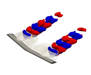
Modes A, B and C for  $(sAR,\varLambda,\alpha,Re)=(4,5^\circ,22^\circ,400)$ visualised with contours of perturbation velocity components at ${\pm }0.1$. The contours of $\bar {u}=0$ in transparent grey and $\bar {u}=-0.1$ in darker grey indicate the recirculation region.

Figure 8 shows the three leading flow eigenmodes on the  $sAR=4$ wing, classified using their frequency, phase and spatial structure. These modes, named A, B and C, are plotted with contours of the three perturbation velocity components for the same wing geometry of $(sAR,\varLambda,\alpha,)=(4,5^\circ,22^\circ )$; in each subplot, both a top and a side view of the same mode are shown. Mode A is the most unstable for most cases examined and takes the form of periodic vortical structures at half-span. As hypothesised in § 4.1, it originates at the peak in the recirculation regions of the base flow. The structure of mode B is visually similar to mode A but with a streamwise drift. It can be seen that both modes A and B originate at the peaks in the recirculation regions of their respective base flows that were shown in figure 6. The $\hat {u}$ and $\hat {w}$ velocity components of modes A and B have two branches, each associated with the shear layer at the top and bottom of the separation bubble, which suggests that these are shear layer instabilities. The vertical $\hat {v}$ velocity component of these modes has a chevron-like structure when viewed from above. However, the peak of the spatial structure of mode A is located near the wing, whereas the structures of mode B become stronger further away from it. Unlike modes A and B that originate at the peaks in the recirculation regions of their respective base flows, mode C has structures just inboard or outboard of the maximum recirculation as shown in the bottom row of figure 8. The contours of $\hat {v}$ velocity of mode C no longer shows a chevron-like pattern, and all velocity components have a row of periodic structures at $2 \leq z \leq 3$ that are oblique to the wing.
Figures 9–11 show the dependence of the frequency and the amplification rate of each of the modes A, B and C on the sweep angle. Figure 12 shows the stable modes present at  $\varLambda =30^\circ$ which was the highest sweep angle considered. In each of these figures, the eigenvalues of a specific mode are highlighted by full symbols and are shown alongside the eigenvalues of other modes to aid visual comparison. As in the figures that showed the base flow, contours of $\bar {u}=0$ in transparent grey and $\bar {u}=-0.1$ in darker grey indicate the recirculation region. The spatial structures of the selected group of modes are shown by labelled contours of $Q=0.5$ in all figures and $St$ is defined as $St=\omega _r c \sin \alpha / 2{\rm \pi} U_{\infty }$.
Spatial structures of mode A at different  $\varLambda$, on a $sAR=4$ wing at a constant $\alpha =22^\circ$, $Re=400$, visualised with contours of $Q=0.5$ shown with top and side view coloured by spanwise vorticity ( $-5\leq \omega _z \leq 5$). An arrow indicates the change of the leading eigenvalue with increasing sweep angle.

Figure 9 shows mode A, which is the leading unstable flow eigenmode in the range  $0^\circ \leq \varLambda \leq 15^\circ$. The plot of $Q$-criterion of mode A for the unswept wing shows periodic vortical structures at half-span. When mirrored in the symmetry plane, the structures of $Q$ have a necklace-like shape when viewed from above. Similar necklace vortices were identified by Taira & Colonius (Reference Taira and Colonius2009) in flows over flat plates. Here, such structures are associated with the leading global eigenmode of a finite wing at different geometrical conditions. This same mode A is the most amplified at $\varLambda =5^\circ$ and $10^\circ$ as can be seen in figure 9. With sweep, the spatial structures of mode A move away from the symmetry plane and towards the tip following the spanwise location of the peak recirculation of the base flow. The frequency remains within $6\,\%$ from the unswept case, but the amplification rate increases by $26\,\%$ from unswept to $\varLambda =10^\circ$. At $\varLambda =15^\circ$, mode A is still dominant, but the spatial structures show some changes. In particular, the lower branch associated with the bottom shear layer is less pronounced when looking from the side, and when viewed from the top the structures show inboard curvature, associated with the shape of the separation bubble near the tip. This might be due to the induced velocity by the tip vortex. Furthermore, under these conditions mode A is about $50\,\%$ less amplified compared to $\varLambda =0^\circ$, which points to a change in the amplification of the leading mode between $\varLambda$ of $10^\circ$ and $15^\circ$. This is attributed to the balance of tip-induced and spanwise flow effects with increasing sweep angle. Both the tip vortex downwash (Zhang et al. Reference Zhang, Hayostek, Amitay, He, Theofilis and Taira2020b) and increased angle of sweep (Zhang et al. Reference Zhang, Hayostek, Amitay, Burtsev, Theofilis and Taira2020a) were shown to have a stabilising effect on the wake. As $\varLambda$ increases, the stabilising effects of the tip decrease, due to the weakening of the tip vortex observed in the flow, leading to mode A being more amplified. As $\varLambda$ increases further, the spanwise flow becomes stronger as discussed in appendix A, and mode A becomes less amplified due to stabilising effect of spanwise flow.
In addition to mode A, which is amplified in all four low-sweep cases shown, a subdominant mode, labelled B shown in figure 10, is also found with the exact same frequency. At  $\varLambda =5^\circ$ and $10^\circ$, mode B is the second most amplified mode and is the third most amplified for $\varLambda =0^\circ$. As mentioned before, mode B closely resembles mode A, however, the structures of modes A and B are out of phase and the two modes have different phase velocities and wavelengths. Just like with mode A, the spanwise location of the peak of mode B moves towards the tip as $\varLambda$ increases, following the peak recirculation of the respective base flow.
Same as figure 9, highlighting mode B.

Mode C, shown in figure 11, has a higher frequency than modes A and B and nearly the same phase velocity as mode B. Unlike the compact structures of modes A and B, the periodic structures of mode C extend further in the spanwise direction. In addition, mode C is not localised at the peak of the separation bubble but also has structures concentrated on either side of it as in the case of  $\varLambda =0^\circ$ and $10^\circ$ or on both sides as in $\varLambda =5^\circ$ and $15^\circ$.
Same as figure 9, highlighting mode C.

No unstable modes were found in the spectrum of the  $\varLambda =30^\circ$ wing. The least-stable mode, labelled D, is stationary and damped. The mode structure shown in figure 12 indicates that it is a vortical structure that counter rotates with respect to the tip vortex. The mode structures follow the direction and spatial location of the spanwise vortices seen in the base flow (figure 6). The second most unstable mode E shown in the same figure peaks further downstream behind the wing with structures showing some resemblance to the wake-like modes A and B but also having vortex-like characteristics.
Same as figure 9 showing modes D and E for  $(sAR,\varLambda,\alpha,Re)=(4,30^\circ,22^\circ,400)$.

Finally, the lower aspect ratio wing ( $sAR=2$) is considered at the same $\alpha =22^\circ$. Global modes for several sweep angles are shown in figure 13. Similar to $sAR=4$ case, the dominant mode for $\varLambda =0^\circ$ and $10^\circ$ is mode A. However, unlike in the higher aspect ratio wing, mode A appears to be less amplified at $\varLambda =10^\circ$, and mode B no longer appears in the spectrum at least up to an Kylov subspace dimension of 50. The fact that mode A does not become more amplified at $\varLambda =10^\circ$ over the $sAR=2$ wing can be explained by stronger tip effects on the shorter wing. At $\varLambda =30^\circ$, the leading mode, labelled F, is steady and takes the form of a tip like instability that was not seen on $sAR=4$ wing. Additional low-frequency travelling and stationary modes are present but are all stable.
Same as figure 9 showing modes A and F on the shorter  $sAR=2$ wing.

The existence of three families of modes that manifest themselves at a range of geometrical configurations is encouraging. Documenting these instabilities at low Reynolds numbers offers a basis for theoretically founded flow control strategies as well as a first step towards understanding turbulent flow at higher Reynolds numbers as it is expected that these modes will exist at range of Reynolds numbers. As mode A, which is dominant for most configurations, is a shear layer instability related to the separation bubble, flow control targeted at the separation bubble could be used to attenuate the formation of wake structures observed in § 4.1 which result from linear growth and the eventual nonlinear saturation of the leading mode as shown in § 4.4. Theoretically founded flow control studies based on solution of the adjoint TriGlobal EVP are currently underway and will be presented elsewhere.
4.3. Effects of Reynolds number and angle of attack
The effect of the Reynolds number on the growth rate and frequency of the leading mode is considered at a fixed set of parameters  $(sAR,\varLambda,\alpha )=(4,0^\circ,22^\circ )$. For the cases where steady flow exists, the residuals algorithm (Theofilis Reference Theofilis2000) was used to extract global mode characteristics from the DNS results, whereas for unstable cases the TriGlobal eigenvalue problem was solved numerically. Consistent results were obtained by the two approaches, the results of which are shown as data points connected by splines. Figure 14(a) presents the dependence of the amplification rate of mode A on Reynolds number and establishes the critical Reynolds number at these conditions, $Re_{{crit}}=180.3$, at which a Hopf bifurcation and the onset of wake unsteadiness occur. The frequency of mode A, shown in figure 14(b), increases before reaching a peak at $Re_{{crit}}$ and decreases afterwards. The growth rate increases nearly lineally in the vicinity of $Re_{{crit}}$ and continues to increase at a lower rate once the flow becomes unstable. As in the case of the two-dimensional cylinder flow (Barkley Reference Barkley2006), at the bifurcation point the frequency of the leading mode matches the wake shedding frequency measured from DNS results, whereas beyond $Re_{{crit}}$ the frequencies diverge. Mean flow stability analysis is needed at Reynolds numbers higher than $Re_{{crit}}$ to recover the shedding frequency as shown in 14(b).
Dependence on  $Re$ of (a) growth rate and (b) frequency of the leading global mode A at $(sAR,\varLambda,\alpha )=(4,0^\circ,22^\circ )$. The DNS shedding frequency is also shown in (b).

Next, the Reynolds number is kept constant at the highest value considered presently,  $Re=400$, and the angle of attack $(\alpha )$ is varied, keeping $sAR$ and $\varLambda$ constant, in order to establish the critical angle of attack $(\alpha _{{crit}})$ at which the flow becomes unstable; results are shown in figure 15. It can be seen that increasing $\alpha$ has a destabilising effect on the flow, the critical angle of attack at these parameters being $\alpha _{{crit}}=13.4^\circ$. Moreover, it can be seen that the amplification rate of the leading global mode plateaus near $\alpha =22^\circ$, whereas its frequency reduces systematically past the critical angle of attack.
Variation of (a) growth rate and (b) frequency of the leading global mode A with  $\alpha$ at $(sAR,\varLambda,Re)=(4,0^\circ,400)$.

The association of the leading three-dimensional global mode with peaks in the reversed streamwise velocity component of the base flow ( $\bar {u}_{{rev}}$) seen in figure 9, calls for examination of the dependence of the latter quantity on the same two variables used in figures 14 and 15. Figure 16 shows the dependence of $\bar {u}_{{rev}}$ on $Re$ and $\alpha$, as a fraction of the free stream velocity. In both cases, the maximum reversed flow increases monotonically when either of $Re$ or $\alpha$ is increased. This growth correlates with the linear slope of the $\omega _i$ curve in the vicinity of the bifurcation point in figures 14(a) and 15(a). The values of recirculation corresponding to the critical conditions $Re_{{crit}}$ and $\alpha _{{crit}}$ are $14\,\%$ and $11\,\%$, respectively. As such, these values fall within the bracket of predictions for absolute instability, $7.5\,\% \le \bar {u}_{{rev}}\le 15\,\%$, obtained by classic absolute/convective instability analysis (Hammond & Redekopp Reference Hammond and Redekopp1998), DNS (Rist & Maucher Reference Rist and Maucher2002) and global stability analysis (Rodríguez & Theofilis Reference Rodríguez and Theofilis2010) of two-dimensional LSB models.
Dependence of the maximum reverse streamwise velocity component on (a)  $Re$ at $(sAR,\varLambda,\alpha )=(4,0^\circ,22^\circ )$ and (b) on $\alpha$ at $(sAR,\varLambda,Re)=(4,0^\circ,400)$. Lines correspond to a least-squares fit of the data points.

4.4. Modal analyses in the nonlinear saturation regime
The evolution of the linearly unstable flows documented in the earlier sections towards nonlinearity is examined next at  $(sAR,\varLambda,\alpha,Re)=(4,5^\circ,22^\circ,400)$. Figure 17 shows the time history at a probe located at $(x,y,z)=(4,0,2)$, whereas the full flow fields are visualised with $Q=1$ coloured by streamwise vorticity $-5 \leq \omega _x \leq 5$. The resulting flow field (EIG) at a time that is well into the nonlinear regime ( $t=60$) is compared with the initial DNS. At early times $t<15$, the flow remains nearly identical to the steady SFD-obtained base flow. At $t\approx 20$, vortical structures emerge at $1 \leq z \leq 2$, corresponding to the spatial locations of the peak of the global mode A. As time evolves, nonlinearity takes over with more complex structures forming in the wake, as seen at $t=30$, with the eventual flow field ( $t=60$) being practically identical to the DNS at corresponding times. The small phase discrepancy is because the times at which the EIG and DNS fields are shown do not exactly match, because the mode takes a long time to grow from the steady flow. The corresponding time for the DNS for this qualitative comparison was chosen such as to approximately match the peaks during nonlinear saturation.
Growth of the global mode for  $(sAR,\varLambda,\alpha,Re)=(4,5^\circ,22^\circ,400)$ showing the time history at point $P(x,y,z)=(4,0,2)$ and flow field evolution at selected times. On the right, the resulting flow field is also compared with the DNS result.

Table 3 presents a quantitative comparison of the frequencies and amplification rates of the leading two modes at different times during the flow evolution: the top two rows show results of the stationary base flow, whereas the middle and lower two rows correspond to the mean flow obtained by time-averaging during nonlinear saturation and to data-driven analyses performed on snapshots, also taken in the nonlinear regime. A number of observations worthy of discussion are made on the basis of these results. First, the growth of the most amplified linearly unstable global mode exactly corresponds to the slope of the logarithmic derivative of the DNS probe data during linear growth. Second, as already seen in figure 14, modes obtained from mean flow stability analysis (Barkley Reference Barkley2006; Sipp & Lebedev Reference Sipp and Lebedev2007) have different frequencies to those of the leading global mode, whereas their amplification rate is close to the theoretically expected value of zero. Third, data-driven analyses (Taira et al. Reference Taira, Brunton, Dawson, Rowley, Colonius, McKeon, Schmidt, Gordeyev, Theofilis and Ukeiley2017) using proper orthogonal decomposition (Lumley Reference Lumley1967; Sirovich Reference Sirovich1987) and dynamic mode decomposition (Schmid & Sesterhenn Reference Schmid and Sesterhenn2008; Rowley et al. Reference Rowley, Mezić, Bagheri, Schlatter and Henningson2009; Schmid Reference Schmid2010) at the nonlinear regime, deliver essentially identical results with those of the corresponding mean flow stability analysis.
Comparison of the frequencies and amplification rates of the first two modes obtained by different methods for  $(sAR,\alpha,Re)=(4,22^\circ,400)$.

Figure 18 shows a visual representation of these results, focusing on the spatial structure of the leading modes obtained using a base flow that satisfies the equations of motion vs their counterparts resulting from mean flow and data-driven stability analyses, all performed at  $(sAR,\varLambda,\alpha,Re)=(4,5^\circ,22^\circ,400)$. Contours of $\bar {u}=0$ in transparent grey and $\bar {u}=-0.1$ in darker grey indicate the recirculation region of the base and mean flows. It can be clearly seen that mean flow modes are distinctly different from the amplified base flow modes and are qualitatively very similar to the modes obtained by data-driven analysis, namely the interaction and wake modes, that will be further discussed in figure 19. In summary, conclusions drawn on the basis of mean flow stability analysis of simpler geometries, namely that the mean flow stability analysis yields neutrally stable perturbations with the frequency of the saturated limit cycle (Barkley Reference Barkley2006; Sipp & Lebedev Reference Sipp and Lebedev2007), are found to carry over in the present fully inhomogeneous three-dimensional flow configuration. The linearly unstable global modes have essentially different spatial distribution of the amplitude functions, as well as different frequencies compared to their counterparts obtained by analysis of the nonlinearly saturated flow regime. The role of the linear eigenmodes identified herein is to connect the steady laminar flow with the nonlinear saturated counterpart through a modal amplification scenario.
Leading modes of (a) base flow, (b) mean flow and (c) data-driven stability analysis for  $(sAR,\varLambda,\alpha,Re)= (4,5^\circ,22^\circ,400)$. Isocontours of modes at $Q=0.5$ coloured by spanwise vorticity $-5 \leq \omega _z \leq 5$.

Data-driven modal results for  $(sAR,\varLambda,\alpha,Re)=(4,5^\circ,22^\circ,400)$ showing (a) the base flow (BF), (b) the interaction mode and (c) the wake mode. Isocontours of base flow at $Q=1$ and modes at $Q=0.5$ coloured by streamwise vorticity $-5 \leq \omega _x \leq 5$.

Figure 19 introduces some qualitative features of the stability analysis results in the nonlinear saturation regime. The two most interesting structures found in the spectrum and corresponding to the mean flow stability analysis results shown in figure 18, are denominated the interaction mode (IM) and the wake mode (WM). The IM, shown in figure 19(b), has vortical structures in the wake reflecting the curvature of the vortices shed from the wing but also has structures corresponding to the interaction region vortices present in the base flow as shown in figure 19(a). On the other hand, WM, shown in figure 19(c), is concentrated in the wake region with structures near the wing being parallel to it. The evolution of these modes with changes in the parameters  $Re$,
$Re$,  $sAR$, $\varLambda$ and $\alpha$ will be discussed in detail elsewhere.
5. Summary
Linear modal three-dimensional (TriGlobal) instability analysis of laminar separated flows over finite aspect ratio, constant-chord wings has been performed at  $100 \leq Re \leq 400$, two aspect ratios and a range of angles of attack and sweep.
Monitoring the unsteady base flows, the following observations were made, as the angle of sweep ( $\varLambda$) increased. When $0^\circ \leq \varLambda < 10^\circ$, the three distinct regions reported by Zhang et al. (Reference Zhang, Hayostek, Amitay, He, Theofilis and Taira2020b) were also observed, namely the tip vortex, wake and the interaction region with braid-like vortices. For $15^\circ \leq \varLambda < 25^\circ$, the braid-like vortices of the interaction region become dominant and absorb the tip vortex. Finally, at $25^\circ \le \varLambda \le 30^\circ$, tip stall and ram's horn vortices are present with steady flow over most of the wing. The overall effect of increasing sweep is flow stabilisation. In the steady flow generated by SFD, a large separation bubble is observed. The spanwise location of the maximum extent of the bubble changes with $\varLambda$ moving towards the tip.
Linear TriGlobal instability analysis was used to identify the critical Reynolds number,  $Re_{{crit}}=180.3$, and critical angle of attack, $\alpha _{{crit}}=13.4^\circ$, on a straight finite wing of ${sAR=4}$. A parametric study of the effect of sweep angle conducted at conditions of maximum unsteadiness, $Re=400$ and $\alpha =22^\circ$, revealed the existence of three families of unstable global modes, denominated A, B and C. Their frequency content and spatial structure were documented for a range of $\varLambda$ and two $sAR$. The leading mode A is dominant in all cases examined, and its most interesting characteristic is that it originates at the peak recirculation zone of the three-dimensional LSB formed on the wing. The latter is located at half-span for an unswept wing and moves towards the wing tip as the angle of attack increases. Mode A follows this spanwise motion of the peak recirculation at all conditions examined. Subdominant modes B and C were also discovered; mode B has practically the same frequency as mode A and also peaks at maximum recirculation but has a different phase velocity. In contrast to the previous two, mode C has a higher frequency, whereas its structure is not localised at the maximum recirculation but extends further in the spanwise direction.
Overall, an increase of the sweep angle was found to stabilise the flow as no globally unstable modes were found at the maximum considered  $\varLambda$ of $30^\circ$. The leading mode at this $\varLambda$ is stable and stationary taking the form of a single vortex tube similar to structures observed in the base flow. This suggests that stabilising effects of spanwise flow are significant only at $\varLambda \gtrsim 10^\circ$, whereas, at lower sweep angles, mode A becomes more amplified due to the weakening of the tip vortex and the reduction of associated stabilising effects. This is not the case for the $sAR=2$ wing, where mode A is already less amplified at $\varLambda =10^\circ$ compared with the unswept case, suggesting a monotonic decrease of the amplification rate with $\varLambda$. This is attributed to the stronger tip effects over the shorter wing. At the highest sweep angle of $30^\circ$ and $sAR=2$, the leading stable mode is a tip instability suggesting that the tip effects are stronger than spanwise flow effects even for high $\varLambda$ on the short wing.
The origin of the wake unsteadiness observed in the simulations of Zhang et al. (Reference Zhang, Hayostek, Amitay, He, Theofilis and Taira2020b) and those performed herein was associated with the unstable global mode A. Exponential growth of mode A superposed upon the underlying steady base flow leads to vortical structures appearing in the DNS results at the same spatial locations where mode A peaks. As time evolves, nonlinearity takes over and more complex structures form in the wake. The variation of the leading mode frequency and growth rate with Reynolds numbers above  $Re_{{crit}}$ is found to be that predicted by Barkley (Reference Barkley2006) on the canonical two-dimensional cylinder: the time-averaged mean flow of the finite wing is neutrally stable and yields the shedding frequency of the wake.
To conclude, linear TriGlobal instability analysis revealed the leading eigenmodes of this class of flows for the first time. The evolution of these modes with aspect ratio and sweep angle was documented. The essential differences between the linear global modes identified herein and those resulting from mean flow (or data-driven) stability analysis has been discussed. This analysis provides insight into the formation of the unstable wake for the range of conditions examined. The results reported here establish a basis for understanding flow dynamics and instabilities on finite three-dimensional untapered wings at low Reynolds numbers, as a first step towards understanding turbulent flow at higher Reynolds numbers.
Acknowledgements
Support of AFOSR Grant FA9550-17-1-0222 with Dr G. Abate and Dr D. Smith as Program Officers is gratefully acknowledged. The authors also acknowledge computational time made available on the UK supercomputing facility ARCHER and ARCHER2 via the UKTC Grant EP/R029326/1 and on the DoD Copper supercomputer, via project AFVAW10102F62 with Dr N. Bisek as Principal Investigator.
Declaration of interests
The authors report no conflict of interest.
Appendix. Effect of  $\varLambda$ on the spanwise flow on the wing

Spanwise flow effects are considered by analysing the time-averaged flow for the  ${\varLambda =5^\circ}$ wing. Figure 20(a) shows isosurfaces of the time-averaged spanwise component of velocity $\langle w \rangle$ at levels from $-0.2$ to $0.2$, on the $(sAR,\varLambda,\alpha,Re)=(4,5^\circ,22^\circ,400)$ wing. A region of positive (towards the tip, shown in red) flow is visible at the leading edge (LE) of the wing as the sweep angle increases. Above the trailing edge (TE), a region of negative (towards the root, shown in blue) flow is seen to peak at $z\approx 2$. Figure 20(b) shows the time-averaged streamwise vorticity $\langle \omega _x \rangle$ behind the wing on the $x=1.5$ plane. As noted by Zhang et al. (Reference Zhang, Hayostek, Amitay, He, Theofilis and Taira2020b), the vortex sheet emanates from the leading edge and the wing tip. The region of negative streamwise vorticity is associated with the roll-up of the wing tip vortex sheet that gives rise to the tip vortex, while the roll-up of the LE vortex sheet leads to a region of positive streamwise vorticity. It can be seen from the velocity vectors in figure 20(b) that these opposing regions of vorticity induce spanwise flow towards the root of the wing in the vicinity of the wing TE. The magnitude of this spanwise flow $|\langle V_{span} \rangle |$ over the TE is compared with spanwise flow towards the tip above the LE in figure 20(c) on a line parallel to the wing and $0.1c$ above the wing. On the $\varLambda =5^\circ$ wing, the induced spanwise flow towards the root is comparable in strength to spanwise flow caused by wing sweep from the quarter-span and nearly all the way to the wing tip, whereas this induced spanwise flow is weaker at larger $\varLambda$ values. This trend holds when lines at various heights above the TE are considered, as is evident in figure 20(d), where the magnitude of opposing spanwise flow is compared at quarter-span ( $z=2$). As the angle of sweep increases, the strength of the tip vortex, and hence spanwise flow towards the root, decreases; by contrast, the spanwise flow at the LE, which is opposite in direction, increases with increasing $\varLambda$. At $\varLambda =5^\circ$ the lines describing the opposite flow motion intersect, suggesting a balance of spanwise and tip-induced flow under these conditions.
(a) Top view of  $(sAR,\varLambda,\alpha )=(4,5^\circ,22^\circ )$ wing showing contours of $\langle w \rangle$. (b) Slice from (a) showing streamwise vorticity and velocity vectors ( $x=1.5$). (c) Magnitude of spanwise flow towards the root (—–) at a line $0.1c$ above the wing TE and towards the tip (- - -) at a line $0.1c$ above the wing LE. (d) Comparison of spanwise flow magnitude towards the root (—–) and tip (- - -) at $z=2$ for lines at different heights ( $y$) above the TE.


 Open access